ELECTRICAL, ELECTRONICS, AND DIGITAL HARDWARE

ESSENTIALS FOR SCIENTISTS AND

ENGINEERS

IEEE Press445 Hoes Lane

Piscataway, NJ 08855

IEEE Press Editorial BoardJohn B. Anderson, Editor in Chief

R. Abhari G. W. Arnold F. CanaveroD. Goldof B-M. Haemmerli D. JacobsonM. Lanzerotti O. P. Malik S. NahavandiT. Samad G. Zobrist

Kenneth Moore, Director of IEEE Book and Information Services (BIS)

ELECTRICAL, ELECTRONICS, AND DIGITAL HARDWARE

ESSENTIALS FOR SCIENTISTS AND

ENGINEERS

Ed LipianskyCisco Systems, Inc.

San Jose, California, USA

IEEE PRESS

A JOHN WILEY & SONS, INC., PUBLICATION

IEEE PRESS SERIES ON MICROELECTRONIC SYSTEMS

Cover Designer: Denise Lipiansky

Copyright © 2013 by The Institute of Electrical and Electronics Engineers, Inc.

Published by John Wiley & Sons, Inc., Hoboken, New Jersey. All rights reservedPublished simultaneously in Canada

No part of this publication may be reproduced, stored in a retrieval system, or transmitted in any form or by any means, electronic, mechanical, photocopying, recording, scanning, or otherwise, except as permitted under Section 107 or 108 of the 1976 United States Copyright Act, without either the prior written permission of the Publisher, or authorization through payment of the appropriate per-copy fee to the Copyright Clearance Center, Inc., 222 Rosewood Drive, Danvers, MA 01923, (978) 750-8400, fax (978) 750-4470, or on the web at www.copyright.com. Requests to the Publisher for permission should be addressed to the Permissions Department, John Wiley & Sons, Inc., 111 River Street, Hoboken, NJ 07030, (201) 748-6011, fax (201) 748-6008, or online at http://www.wiley.com/go/permissions.

Limit of Liability/Disclaimer of Warranty: While the publisher and author have used their best efforts in preparing this book, they make no representations or warranties with respect to the accuracy or completeness of the contents of this book and specifically disclaim any implied warranties of merchantability or fitness for a particular purpose. No warranty may be created or extended by sales representatives or written sales materials. The advice and strategies contained herein may not be suitable for your situation. You should consult with a professional where appropriate. Neither the publisher nor author shall be liable for any loss of profit or any other commercial damages, including but not limited to special, incidental, consequential, or other damages.

For general information on our other products and services or for technical support, please contact our Customer Care Department within the United States at (800) 762-2974, outside the United States at (317) 572-3993 or fax (317) 572-4002.

Wiley also publishes its books in a variety of electronic formats. Some content that appears in print may not be available in electronic formats. For more information about Wiley products, visit our web site at www.wiley.com.

Library of Congress Cataloging-in-Publication Data:

Lipiansky, Ed. Electrical, electronics, and digital hardware essentials for scientists and engineers / Ed Lipiansky. p. cm. ISBN 978-1-118-30499-0 (hardback) 1. Electronic circuits. 2. Electronic apparatus and appliances. I. Title. TK7876.L484 2012 621.3–dc23 2012012321

Printed in the United States of America

10 9 8 7 6 5 4 3 2 1

To my lovely wife Ruty

CONTENTS

Preface xvii

AbouttheAuthor xix

1 FromtheBottomUp:Voltages,Currents,andElectricalComponents 1

1.1 AnIntroductiontoElectricChargesandAtoms / 11.2 ElectricDCVoltageandCurrentSources / 3

1.2.1 ElectricCurrentandVoltage / 31.2.2 DCVoltageandCurrentSources / 51.2.3 SourcesInternalResistance / 9

1.3 ElectricComponents:Resistors,Inductors,andCapacitors / 121.3.1 Resistors / 121.3.2 ResistorsinSeriesandinParallel / 191.3.3 Resistivity:APhysicalInterpretation / 231.3.4 ResistanceofConductors / 25

1.4 Ohm’sLaw,PowerDeliveredandPowerConsumed / 251.4.1 VoltageSourceInternalResistance / 30

1.5 Capacitors / 331.5.1 PhysicalInterpretationofaParallel-PlateCapacitor

Capacitance / 351.5.2 CapacitorVoltageCurrentRelationship / 361.5.3 CapacitorsinSeries / 371.5.4 CapacitorsinParallel / 391.5.5 EnergyStoredinaCapacitor / 401.5.6 RealCapacitorParametersandCapacitorTypes / 41

1.6 Inductors / 441.6.1 Magnetism / 451.6.2 MagneticFieldaroundaCoil / 491.6.3 MagneticMaterialsandPermeability / 521.6.4 ElectromagneticInductionandInductorCurrent–Voltage

Relationship / 53

vii

viii    CONTENTS

1.6.5 InductorsinSeries / 581.6.6 InductorsinParallel / 601.6.7 MutualInductance / 621.6.8 EnergyStoredbyanInductor / 691.6.9 InductorNonlinearity / 701.6.10 InductorComponentSelection / 71

1.7 Kirchhoff’sVoltageLaw(KVL)andKirchhoff’sCurrentLaw(KCL) / 73

1.8 Summary / 87FurtherReading / 87Problems / 88

2 AlternatingCurrentCircuits 98

2.1 ACVoltageandCurrentSources,RootMeanSquareValues(RMS),andPower / 982.1.1 IdealandRealACVoltageSources / 992.1.2 IdealandRealACCurrentSources / 106

2.2 SinusoidalSteadyState:TimeandFrequencyDomains / 1112.2.1 ResistorunderSinusoidalSteadyState / 1122.2.2 InductorunderSinusoidalSteadyState / 1122.2.3 CapacitorunderSinusoidalSteadyState / 1132.2.4 BriefComplexNumberTheoryFacts / 115

2.3 TimeDomainEquations:FrequencyDomainImpedanceandPhasors / 1232.3.1 Phasors / 1232.3.2 TheImpedanceConcept / 1242.3.3 PurelyResistiveImpedance / 1262.3.4 InductiveImpedance:InductiveReactance / 1272.3.5 PurelyCapacitiveImpedance:Capacitive

Reactance / 1312.3.6 R,L,andCImpedancesCombinations / 133

2.4 PowerinACCircuits / 1362.4.1 ACInstantaneousPowerDrawnbyaResistor / 1372.4.2 ACInstantaneousPowerDrawnbyaCapacitor / 1372.4.3 ACInstantaneousPowerDrawnbyanInductor / 139

2.5 DependentVoltageandCurrentSources / 1452.5.1 Voltage-ControlledVoltageSource(VCVS) / 1452.5.2 Current-ControlledVoltageSource(CCVS) / 1462.5.3 Voltage-ControlledCurrentSource(VCCS) / 1472.5.4 Current-ControlledCurrentSource(CCCS) / 148

2.6 SummaryofKeyPoints / 149FurtherReading / 149Problems / 150

CONTENTS    ix

3 CircuitTheoremsandMethodsofCircuitAnalysis 155

3.1 Introduction / 1553.2 TheSuperpositionMethod / 156

3.2.1 CircuitsSuperposition / 1603.3 TheThéveninMethod / 165

3.3.1 ApplicationoftheThéveninMethod / 1673.4 Norton’sMethod / 172

3.4.1 SourceTransformations / 1743.4.2 FindingtheNortonEquivalentCircuitDirectlyfrom

theGivenCircuit / 1753.5 TheMeshMethodofAnalysis / 179

3.5.1 EstablishingMeshEquations.CircuitswithVoltageSources / 180

3.5.2 EstablishingMeshEquationsbyInspectionoftheCircuit / 186

3.5.3 EstablishingMeshEquationsWhenThereArealsoCurrentSources / 189

3.5.4 EstablishingMeshEquationsWhenThereArealsoDependentSources / 196

3.6 TheNodalMethodofAnalysis / 1993.6.1 EstablishingNodalEquations:CircuitswithIndependent

CurrentSources / 1993.6.2 EstablishingNodalEquationsbyInspection:

CircuitswithCurrentSources / 2013.6.3 EstablishingNodalEquationsWhenThereArealso

VoltageSources / 2053.6.4 EstablishingNodalEquationsWhenThereAre

DependentSources / 2073.7 WhichOneIstheBestMethod? / 210

3.7.1 SuperpositionTheoremHighlights / 2103.7.2 ThéveninTheoremHighlights / 2113.7.3 Norton’sTheoremHighlights / 2113.7.4 SourceTransformationsHighlights / 2123.7.5 MeshMethodofAnalysisHighlights / 2123.7.6 NodalMethodofAnalysisHighlights / 212

3.8 UsingalltheMethods / 2133.8.1 SolvingUsingSuperposition / 2133.8.2 Example3.21:SolvingtheCircuitofFigure3.36

byThévenin / 2163.8.3 Example3.22:SolvingtheCircuitofFigure3.36

byNorton / 2193.8.4 Example3.23:SolvingtheCircuitofFigure3.36

UsingSourceTransformations / 221

x    CONTENTS

3.8.5 Example3.24:SolvingtheCircuitofFigure3.36UsingtheMeshMethod / 223

3.8.6 Example3.25:SolvingtheCircuitofFigure3.36UsingtheNodalMethod / 224

3.9 SummaryandConclusions / 225FurtherReading / 225Problems / 226

4 First-andSecond-OrderCircuitsunderSinusoidalandStepExcitations 233

4.1 Introduction / 2334.2 TheFirst-OrderRCLow-PassFilter(LPF) / 235

4.2.1 FrequencyDomainAnalysis / 2354.2.2 BriefIntroductiontoGainandthe

Decibel(dB) / 2364.2.3 RCLPFMagnitudeandPhaseBodePlots / 2384.2.4 RCLPFDrawingaBodePlotUsingJust

theAsymptotes / 2414.2.5 InterpretationoftheRCLPFBodePlotsin

theTimeDomain / 2444.2.6 WhyDoWeCallThisCircuitaLPF? / 2454.2.7 TimeDomainAnalysisoftheRCLPF / 2454.2.8 First-orderRCLPFunderPulseandSquare-Wave

Excitation / 2484.2.9 TheRCLPFasanIntegrator / 251

4.3 TheFirst-OrderRCHigh-PassFilter(HPF) / 2524.3.1 RCHPFFrequencyDomainAnalysis / 2534.3.2 DrawinganRCHPFBodePlotUsingJustthe

Asymptotes / 2544.3.3 InterpretationoftheRCHPFBodePlotsin

theTimeDomain / 2574.3.4 WhyDoWeCallThisCircuitanHPF? / 2584.3.5 TimeDomainAnalysisoftheRCHPF / 2584.3.6 First-OrderRCLPFunderPulseandSquare-Wave

Excitation / 2604.3.7 TheRCHPFasaDifferentiator / 263

4.4 Second-OrderCircuits / 2654.5 SeriesRLCSecond-OrderCircuit / 2664.6 Second-OrderCircuitinSinusoidalSteadyState:

BodePlots / 2754.7 DrawingtheSecond-OrderBodePlotsUsingAsymptotic

Approximations / 2784.8 Summary / 279FurtherReading / 279Problems / 280

CONTENTS    xi

5 TheOperationalAmplifierasaCircuitElement 287

5.1 IntroductiontotheOperationalAmplifier / 2875.2 IdealandRealOpAmps / 2885.3 BriefDefinitionofLinearAmplifiers / 2905.4 LinearApplicationsofOpAmps / 294

5.4.1 TheInvertingAmplifier / 2945.4.2 TheNoninvertingAmplifier / 3065.4.3 TheBufferorNoninvertingAmplifierofUnity

Gain / 3095.4.4 TheInvertingAdder / 3145.4.5 TheDifferenceAmplifier / 3165.4.6 TheInvertingIntegrator / 3215.4.7 TheInvertingDifferentiator / 3225.4.8 APracticalIntegratorandDifferentiatorCircuit / 326

5.5 OpAmpsNonlinearApplications / 3315.5.1 TheOpen-LoopComparator / 3325.5.2 PositiveandNegativeVoltage-LevelDetectorsUsing

Comparators / 3325.5.3 ComparatorwithPositiveFeedback(Hysteresis) / 336

5.6 OperationalAmplifiersNonidealities / 3415.7 OpAmpSelectionCriteria / 3435.8 Summary / 347FurtherReading / 348Problems / 348AppendixtoChapter5 / 353

6 ElectronicDevices:Diodes,BJTs,andMOSFETs 354

6.1 IntroductiontoElectronicDevices / 3546.2 TheIdealDiode / 355

6.2.1 TheHalf-WaveRectifier / 3576.2.2 TheFull-WaveBridgeRectifier / 3606.2.3 TheRealSiliconDiodeI-VCharacteristics:Forward-Bias,

Reverse-Bias,andBreakdownRegions / 3636.2.4 TwoMoreRealisticDiodeModels / 3676.2.5 Photodiode / 3696.2.6 LightEmittingDiode(LED) / 3696.2.7 Schottky-BarrierDiode / 3716.2.8 AnotherDiodeApplication:LimitingandClamping

Diodes / 3716.2.9 DiodeSelection / 372

6.3 BipolarJunctionTransistors(BJT) / 3746.3.1 BasicConceptsonIntrinsic,n-typeandp-typeSilicon

Materials / 3746.3.2 TheBJTasaCircuitElement / 376

xii    CONTENTS

6.3.3 BipolarTransistorI-VCharacteristics / 3776.3.4 BiasingTechniquesofBipolarTransistors / 3826.3.5 VerySimpleBiasing / 3856.3.6 ResistorDividerBiasing / 3876.3.7 EmitterDegenerationResistorBiasing / 3916.3.8 Self-BiasedStaged / 3946.3.9 BiasingTechniquesofPNPBipolarTransistors / 3966.3.10 SmallSignalModelandSingle-StageBipolarAmplifier

Configurations / 3976.3.11 CommonEmitter(CE)Configuration / 3996.3.12 CommonEmitter(CE)ConfigurationwithEmitter

Degeneration / 4046.3.13 Common-Base(CB)Configuration / 4076.3.14 TheCommon-Collector(CC)Configuration / 415

6.4 MetalOxideFieldEffectTransistor(MOSFET) / 4206.4.1 MOSFETI-VCharacteristics / 4246.4.2 MOSFETSmallSignalModel / 4276.4.3 MOSFETBiasingTechniques / 4286.4.4 CommonSource(CS)Configuration / 4346.4.5 CommonSource(CS)Configurationwith

Degeneration / 4366.4.6 CommonGate(CG)Configuration / 4376.4.7 CommonDrain(CD)ConfigurationorSource

Follower / 4396.4.8 OtherMOSFETs:EnhancementModep-Channeland

DepletionMode(n-Channelandp-Channel) / 4396.5 Summary / 443FurtherReading / 446Problems / 446

7 CombinationalCircuits 456

7.1 IntroductiontoDigitalCircuits / 4567.2 BinaryNumbers:aQuickIntroduction / 4567.3 BooleanAlgebra / 460

7.3.1 ANDLogicOperation 4607.3.2 ORLogicOperation(AlsoCalledInclusiveOR,

orXNOR) / 4617.3.3 NOTLogicOperationorInversion—NAND

andNOR / 4627.3.4 ExclusiveORLogicOperationorXOR / 4637.3.5 DeMorgan’sLaws,Rules,andTheorems / 4647.3.6 OtherBooleanAlgebraPostulatesandTheorems / 4657.3.7 TheDualityPrinciple / 4667.3.8 VennDiagrams / 467

CONTENTS    xiii

7.4 Minterms:StandardorCanonicalSumofProducts(SOP)Form / 467

7.5 Maxterms:StandardorCanonicalProductofSums(POS)Form / 472

7.6 KarnaughMapsandDesignExamples / 4737.6.1 Two-VariableKarnaughMaps / 4747.6.2 Three-VariableKarnaughMaps / 4797.6.3 Four-VariableKarnaughMaps / 4847.6.4 Five-VariableKarnaughMaps / 487

7.7 ProductofSumsSimplifications / 4907.8 Don’tCareConditions / 4917.9 LogicGates:ElectricalandTimingCharacteristics / 495

7.9.1 GatesKeyElectricalCharacteristics / 4977.9.2 GatesKeyTimingCharacteristics / 499

7.10 Summary / 500FurtherReading / 500Problems / 500

8 DigitalDesignBuildingBlocksandMoreAdvancedCombinationalCircuits 503

8.1 CombinationalCircuitswithMorethanOneOutput / 5038.2 DecodersandEncoders / 510

8.2.1 MakingLargerDecoderswithSmallerOnes / 5158.2.2 Encoders / 517

8.3 MultiplexersandDemultiplexers(MUXesandDEMUXes) / 5198.3.1 Multiplexers / 5218.3.2 BuildingLargerMultiplexers / 5228.3.3 De-Multiplexers / 526

8.4 SignedandUnsignedBinaryNumbers / 5278.4.1 One’sComplementRepresentationofBinaryNumbers:

Addition / 5278.4.2 Two’sComplementRepresentationofBinaryNumbers:

Addition / 5318.4.3 OtherNumberingSystems / 533

8.5 ArithmeticCircuits:Half-Adders(HA)andFull-Adders(FA) / 5338.5.1 BuildingLargerAdderswithFull-Adders / 5368.5.2 NotesaboutFull-AdderTiming / 5408.5.3 Subtractingwitha4-bitAdderUsing1’sComplement

Representation / 5408.5.4 Subtractingwitha4-bitAdderUsing2’sComplement

Representation / 542

xiv    CONTENTS

8.6 CarryLookAhead(CLA)orFastCarryGeneration / 5438.7 SomeShort-HandNotationforLargeLogicBlocks / 5468.8 Summary / 547FurtherReading / 548Problems 548

9 SequentialLogicandStateMachines 550

9.1 Introduction / 5509.2 LatchesandFlip-Flops(FF) / 552

9.2.1 NAND-ImplementedR– / S–Latch / 5579.2.2 SR-LatchwithEnable / 5599.2.3 Master/SlaveSR-Flip-Flop / 5619.2.4 Master/SlaveJKFlip-Flop / 5659.2.5 Master/SlaveTandDTypeFlip-Flops / 568

9.3 TimingCharacteristicsofSequentialElements / 5719.3.1 TimingofFlip-FlopswithAdditionalSetandReset

ControlInputs / 5719.4 SimpleStateMachines / 574

9.4.1 SRFlip-FlopExcitationTable / 5789.4.2 TFlip-FlopExcitationTable / 5809.4.3 DFlip-FlopExcitationTable / 581

9.5 SynchronousStateMachinesGeneralConsiderations / 5929.5.1 SynchronousStateMachineDesignGuidelines / 5929.5.2 TimingConsiderations:LongandShortPath

Analyses / 5959.6 Summary / 599FurtherReading / 600Problems / 600

10 ASimpleCPUDesign 603

10.1 OurSimpleCPUInstructionSet / 60310.2 InstructionSetDetails:RegisterTransferLanguage(RTL) / 60510.3 BuildingaSimpleCPU:ABottom-UpApproach / 607

10.3.1 TheRegisters / 60710.3.2 TheMemoryAccessPathorMemoryInterface / 61010.3.3 TheArithmeticandLogicUnit(ALU) / 61110.3.4 TheProgramCounter(PC) / 611

10.4 DataPathArchitecture:PuttingtheLogicBlocksTogether / 61510.4.1 DataPath:LDAInstructionFetch,Decodeand

ExecutionRTL / 61510.4.2 AllOtherInstructions:Fetch,DecodeandExecution:

RTL / 618

CONTENTS    xv

10.5 TheSimpleCPUController / 62010.5.1 StateAssignmentsandControllerImplementation / 622

10.6 CPUTimingRequirements / 62610.7 OtherSystemPieces:Clock,ResetandPowerDecoupling / 628

10.7.1 Clock / 62810.7.2 Reset / 62810.7.3 PowerDecoupling / 631

10.8 Summary / 633FurtherReading / 633Problems / 633

Index 637

PREFACE

For several years I taught an introductory analog and digital essentials course for the University of California Extensions at Berkeley and Santa Cruz. Teach-ing there motivated me to put together, under one cover, a textbook that contains fundamentals of electrical, electronics, analog, and digital circuits. That is the reason for the word “essentials” in the title. There are not that many books in the market that try to accomplish this task in about 600 pages.

The book is divided into 10 chapters. It is useful for surveys of electrical and electronics courses, for college students as well as practicing scientists and engineers; it is also useful for introductory circuit courses at the undergraduate level. The book provides many examples from beginning to end. Within the examples, specific components part numbers were avoided to prevent this book from becoming obsolete. The book can be used by students who have some to no previous knowledge of the material, and for graduate-level and working professionals’ circuit courses. The prerequisites for using this book are freshman-level calculus and algebra. Nevertheless, the level of math needed is quite light. The book is a gentle introduction to electrical and electronic circuit analysis with many examples.

Physical concepts are emphasized not only with text but also with specially prepared figures that should help the first-time readers study the material.

This book emphasizes problem solving, using different circuit analysis meth-odologies. These techniques allow readers to understand when one method is more appropriate than another. Ultimately, it is the student who is responsible for adopting the methods that make the most sense. No one thinks exactly in the same way. An example is differentiation and integration. For some people, differentiation is simpler than integration; for others, is the other way around.

Chapter 1 covers the three basic circuit elements: resistors, inductors, and capacitors. Additionally, ideal and real independent DC current and voltage sources are addressed. Chapter 2 emphasizes AC circuits, as they are applied to the three basic circuit elements. Their time-domain and frequency-domain behavior is seen throughout examples. A brief refresher on operations with complex numbers is embedded in this chapter and not in an appendix for reasons of reading continuity. The concept of power drawn by a circuit and its different types are addressed. The chapter ends with the coverage of dependent

xvii

xviii    PREFACE

voltage and current sources. Chapter 3 addresses methods to solve circuits; it should be studied with the greatest attention and as many problems with dif-ferent circuit analysis methods as possible should be solved. From a practical point of view, this is a core chapter to master.

Chapter 4 describes with plenty of detail the behavior of first-order and second-order circuits in the time and frequency domains. Many textbooks do not put as much emphasis on first-order circuits, because they are considered too simple. It has been my experience with students that first-order high-pass filters are particularly more difficult to understand than first-order low-pass filters. Chapter 5 is dedicated to operational amplifiers. Even though op amps consist of to-be-covered electronic components, it is useful to have the reader think with some high level of abstraction. Under some conditions op amps are seen as func-tional blocks and not as circuits with transistors and resistors. Linear and nonlin-ear applications with op amps are covered with many examples.

Chapter 6 covers electronic devices. Much information on devices is pro-vided. One can say that entire books have been written just on the electronic components addressed by this chapter. The textbook takes a systematic approach to study the circuits using diodes and transistors, hardly dwelling on device physics. Chapter 7 begins with digital logic. Combinational (and not “combinatorial,” as it is sometimes mistakenly called) logic circuits do not have any memory. Logic operations or Boolean algebra is presented, and logic simplification methods such as the Karnaugh map method are illustrated. Chapter 8 deals with more advanced combinational circuits such as multiplex-ers, decoders, and some arithmetic circuits. A method to produce a very fast arithmetic sum of two operands is covered. Chapter 9 is about state machine design or sequential logic. Sequential logic has memory, unlike combinational logic, and it is the core subject when designing logic circuits that perform useful and complete functions. Chapter 10 describes piece by piece the construction of a simple CPU. The CPU basic functional blocks, such as its instruction set, the data path architecture, its memory interface, and the control logic, are described step by step. Some insights into capacitor power decoupling and reliable reset circuits are also presented. The problems at the end of this chapter provide tremendous insight into the CPU functionality. This chapter can be thought as a very light introduction to a computer architecture course.

Writing this book has been a very rewarding experience for me. This book should be very useful to college students and those professionals who need an essential analog and digital source.

I want to thank my wife Ruty and daughter Denise for their infinite patience and support while I was preparing the manuscript.

Eduardo (Ed) M. Lipiansky

ABOUT THE AUTHOR

Eduardo (Ed) Lipiansky received his undergraduate degree in electrical engi-neering from the National University of La Plata, Argentina (UNLP). He performed graduate studies at the University of California, Berkeley, obtain-ing a master of science degree in electrical engineering. Mr. Lipiansky has 25 years of industry experience, having worked at Varian Associates, Tandem Computer, Sun Microsystems, Cisco Systems, and Google.

He is author or co-author of six patents; four have been issued by the U.S. Patent Office, and two more have been submitted. Mr. Lipiansky’s key inter-ests are maintenance and diagnostics subsystems for servers, networking line cards, analog and digital electronic design for medical instrumentation and computers, and power engineering. Ed wrote Embedded Systems Hardware for Software Engineers (2011), which deals with more advanced hardware concepts and can be used as an add-on to the present textbook. For about 20 years, he taught a variety of courses such as circuit analysis, digital design, operational amplifiers, and microprocessor interfacing techniques at the Uni-versity of California Berkeley and Santa Cruz Extensions. Mr. Lipiansky lives with his family in the San Francisco Bay area in northern California.

xix

1

1FROM THE BOTTOM UP: VOLTAGES, CURRENTS,

AND ELECTRICAL COMPONENTS

1.1  AN INTRODUCTION TO ELECTRIC CHARGES AND ATOMS

The ancient Greek philosophers knew that when amber was rubbed against wool, it would attract lightweight particles of other materials like small pieces of paper or lint. Also, little pieces of paper get attracted to a plastic comb when the weather is dry. These experiments reveal that electric charge exists. If we rub one end of a glass rod with silk, charges will move toward that end of the rod. Rubbing a second glass rod in the same fashion and placing it close to the rubbed end of the first glass rod will exhibit a repelling force between the rods. However, when a plastic rod is rubbed with fur and it is placed near the rubbed glass rod, the plastic and the glass rods will attract each other. These simple experiments prove the existence of two different types of charge. Benjamin Franklin* called one of them positive and the other one negative. Most charge in an everyday object appears to be nonexistent because there is an equal amount of positive and negative charge. The word electron is derived from the Greek word “elektron,” which means amber. From the above experiments the following can be asserted:

Charges of the same sign repel each other, while charges of opposite signs attract each other.

Electrical, Electronics, and Digital Hardware Essentials for Scientists and Engineers, First Edition. Ed Lipiansky.© 2013 The Institute of Electrical and Electronics Engineers, Inc. Published 2013 by John Wiley & Sons, Inc.

* Benjamin Franklin: American scientist, writer, and politician (1706–1790).

2 FROM THE BOTTOM UP: VOLTAGES, CURRENTS, AND ELECTRICAL COMPONENTS

All matter is made of the basic elements, those elements listed in the periodic table of chemical elements. As of 2006, there are 117 elements of which 94 are found naturally on the Earth. The remaining elements are synthesized in par-ticle accelerators. Loosely speaking, all matter is made of some combination of atoms, where an atom is the basic unit of matter. An atom contains a nucleus surrounded by a cloud of electrons. The nucleus consists of positively charged protons and electrically neutral neutrons. Neutrons have no electrical charge, but their mass is about 1800 times the mass of electrons. The electronic cloud around the nucleus is negatively charged, and an atom with an equal number of protons and electrons is said to be neutral. Protons have a positive charge and a mass about 1800 times larger than the mass of electrons. Different element atoms are different from each other because of the different numbers and arrangements of the atom’s basic particles: electrons, neutrons, and protons. Traditionally in elementary physics and chemistry, the atom was compared to our planetary system. The nucleus is in the center of the atom, like the sun is the center of our system. The electrons are like the planets, orbiting around the sun. Electrons occupy different layers or shells that are at different dis-tances away from nucleus. The outermost shell is referred to as the valence shell. The valence shell electrons determine the electrical characteristics of an atom.

Table 1.1 presents the elementary charge, which has a positive sign for a proton and a negative sign for an electron. Values for the mass of the electron, proton, and neutron are also tabulated.

From an electrical point of view, there are four main types of materials: conductors, nonconductors or insulators, semiconductors, and superconduc-tors. The fourth type of material, the superconductor, is beyond the scope of this book.

Conductors are materials through which charge can move quite freely, such as copper or gold. Insulators are materials through which charge cannot move freely such as plastic or rubber. Semiconductors are materials that have an intermediate behavior between that of conductors and insulators. More on semiconductors will be covered in Chapter 6.

Table 1.1  Some atomic constants

Abbreviation Mass Value Units

Relative Mass to the Electron

Mass (me)Charge in C (coulombs)

Elementary charge

e 1.602 × 10−19

Electron me 9.109 × 10−31 kg 1 −1.602 × 10−19

Proton mp 1.673 × 10−27 kg 1800 (approx.) +1.602 × 10−19

Neutron mn 1.675 × 10−27 kg 1800 (approx.) 0

ELECTRIC DC VOLTAGE AND CURRENT SOURCES 3

1.2  ELECTRIC DC VOLTAGE AND CURRENT SOURCES

Two types of independent sources are available, voltage and current sources. A source is said to be independent when either its nominal voltage or current is constant and does not depend on any other voltage or current present in a circuit. In a later section, we will cover the concept of dependent sources. The ideal voltage source produces a constant voltage across its terminals, regard-less of the current that is being drawn from it by a load. Conversely, an ideal current source produces a constant current to a load connected across its terminals regardless of the voltage that is developed across the load. Let us now address the concepts of electric current and voltage.

1.2.1  Electric Current and Voltage

A net flow of electric charges through a circuit establishes an electric current. Note that conductors in isolation, such as a piece of copper not connected to anything else, contain free electrons or conduction electrons that randomly move. Such electrons do not constitute an electric current since in any cross section of the copper wire, the net amount of charge moved through the wire is zero. The emphasis here is on the word “net”; the net flow of charge consti-tutes an electric current. Current is defined as

i tdqdt

( ) ,= (1.1)

where i(t) represents electric current as a function of time and dq/dt is the net variation of charge with respect to time. Traditionally, electric current was referred to as current intensity. In most places, the term “current” is used, which is a short form of current intensity. The letter i denotes current, while dq differential of charge over dt differential of time refers to the net passage of charge during a time interval through a cross section of the conductor. On the other hand, a voltage can be interpreted as the “pressure” that needs to be asserted in a circuit in order to cause electric current to flow.

Throughout the book, we will assume that a conductor or a wire is ideal and will have zero resistance to the flow of current, unless it is stated otherwise. The unit of resistance is the ohm (Ω). Electric components that have greater than 0 Ω resistance are called resistors. The current that flows through a resis-tor times the resistance value equals the voltage drop that is produced across such resistor. Conventional current in a resistor flows from higher voltages or potentials to lower voltages or potentials.

Figure 1.1 depicts a resistor, a current flowing through it, and the voltage with its polarities that is produced across the resistor. The current through the resistor times its resistance value equals the voltage obtained across the resis-tor terminals. Mathematically,

4 FROM THE BOTTOM UP: VOLTAGES, CURRENTS, AND ELECTRICAL COMPONENTS

V IR= . (1.2)

Equation (1.2) states the voltage across a resistor is proportional to the current flowing through it. The constant of proportionality is the resistor value R. Equation (1.2) is Ohm’s Law. In Figure 1.1a, a resistor powered by a DC source is shown; Figure 1.1b depicts the variation of resistor voltage versus current variation. The slope of the line V = I R is the resistance value. Ohm’s law in Equation (1.2) denotes a linear variation of the voltage across the resis-tor versus the current flowing through it.

Figure 1.1  Ohm’s Law: (a) DC voltage source powering a resistor; (b) linear variation of resis-tor voltage versus current.

RV+

_

+

_

I

V (V )

I (A)

R = DV

DV

DIDI

/

V = I . R

Slope

(a)

(b)

ELECTRIC DC VOLTAGE AND CURRENT SOURCES 5

1.2.2  DC Voltage and Current Sources

We all have some familiarity with electricity and electronics. We have seen flashlights, batteries, battery chargers, lightbulbs, portable electronic devices, and electrical and electronic appliances such as toasters and microwave ovens.

Flashlight batteries, toy batteries, and automobile batteries are all examples of DC voltage sources. DC stands for direct current, and what this means is that the current polarity that the source supplies does not change; that is, the current always flows in the same direction through the load.

An idealization of the DC voltage source is that its DC voltage is always constant with respect to time and independent of the amount of current that it may supply. In practical devices such as batteries, that voltage is “somewhat” constant, and it varies based on factors such as temperature, environmental factors, mechanical vibration, age of the battery, and use of the battery. However, unless we state otherwise, the first-order approximation of a battery is that of a constant or DC voltage source.

Current sources are as also idealized like DC voltage sources. An everyday example of a current source is a battery charger. A battery charger provides a constant current to recharge a battery with rechargeable chemistry. Note that not all batteries are rechargeable. No attempt should be made to recharge batteries that are not of the rechargeable kind, since this causes a hazard to the user. Another example of a current source is that of a transistor hooked up to operate as a current source.

A DC voltage source may not always be a chemical battery. It may, for example, be built with electronic components that behave largely like a DC source. An example of this is a DC power supply (see Figure 1.2).

When a DC voltage source is not being used, it must be stored in an open-circuit condition (refer to Figure 1.3a). That means nothing is connected to the positive and the negative electrical terminals. Upon connecting an element

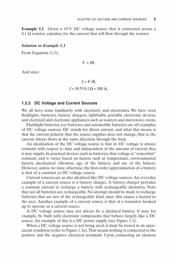
Example 1.1 Given a 10-V DC voltage source that is connected across a 0.1 Ω resistor, calculate for the current that will flow through the resistor.

Solution to Example 1.1

From Equation (1.2),

V IR= .

And since

I V R= / ,

I = =1 V/ 1 A0 0 1 00. .Ω

6 FROM THE BOTTOM UP: VOLTAGES, CURRENTS, AND ELECTRICAL COMPONENTS

such as a lightbulb across the voltage source terminals, a current flows through the circuit that was just established. Figure 1.3b shows a DC voltage source, which in this case is actually a battery connected with wires to a lightbulb.

The battery exerts “pressure” into the circuit by displacing charges. The net flow of charge with respect to time is called an electric current. Physically, an electric current consists of a net flow of electrons. That is, the electronic current leaves the negative terminal of the source, goes through the lightbulb, and returns back into the positive terminal of the source. However, the traditional interpretation is that current flows from the positive terminal of the source through the lightbulb and back into the negative terminal of the source. Throughout this book, the traditional or conventional current flow will be used. This is what most of the electrical engineering literature assumes.

Figure 1.2  Mathematical representation of a DC voltage source as a function of time.

VoltageMagnitude

V = Constant

time

(V )

(sec)

Figure 1.3  DC voltage source in (a) open-circuit condition and (b) loaded with a lightbulb.

LAMPV+

_

+

_

+

_V

I

(a) (b)

ELECTRIC DC VOLTAGE AND CURRENT SOURCES 7

The lightbulb depicted in Figure 1.3 is in effect a resistor. The voltage applied and the resistance of the lightbulb determines the current that will be present in the closed circuit. Resistance is the opposition that a resistor pres-ents to the net flow of current. In other words, the DC voltage source voltage is basically constant, regardless of the amount of current that is being drawn form the source. Naturally, this is an idealization of what a DC voltage source is, or what we would like it to be. Real voltage sources do not behave that way; their output voltage is quite constant as long as the current flowing through the circuit is considerably less than what the total current pumping capability of the source is. More details on this topic will be provided when the internal resistance of a source is addressed, later in this chapter.

DC current sources, on the other hand, produce a constant current when a lightbulb or a resistive element establishes a closed loop circuit and the voltage across it will depend strictly on the resistive value placed across the current source and the current value. Just like with the DC voltage source, the DC current source is an idealization. Real current sources can provide a constant current as long as the voltage across the resistor does not produce an excessive voltage. Figure 1.4 depicts a constant DC current as a function of time.

Figure 1.5a depicts a DC current source in a standby condition, that is, with its terminals short-circuited to each other. A current source should not be left open-circuited because the voltage that gets developed across its terminals would grow without bound. A real or physical current source would self-destruct or become severely damaged if its terminals were left in an open-circuit condition. Figure 1.5b depicts a DC current source with a resistor connected across its terminals. In Figure 1.5a,b, both states of the current source are benign states or normal states. In both cases, the current supplied by the current source is identical.

Figure 1.4  Mathematical representation of a DC current source as a function of time.

Magnitude

I =

I = Current

Constant

time

(A)

(sec)

8 FROM THE BOTTOM UP: VOLTAGES, CURRENTS, AND ELECTRICAL COMPONENTS

The ideal current source with a resistive element in a closed circuit (Fig. 1.5) provides a constant current, and the voltage across the terminals of the current source depends on the value of the resistor across the current source times the current supplied by the source. Changes of the resistor values across the current source will produce proportional changes of the voltage across the current source. Note that the resistor (or load) across a current source pro-duces higher voltages as the load resistor increases in value, because the current remains constant. For the case that the load resistor is very large, the voltage across the current source will be very large. When current sources are in open-circuit condition, the voltage across its terminal grows without bound. Real current sources would self-destruct quickly under an open-circuit condi-tion. The current source must always be short-circuited when not in use (refer to Figure 1.5a). The voltage across a shorted current source is zero because the wire across the current source has zero resistance. However, the current

Figure 1.5  DC current source (a) in short-circuit condition and (b) loaded with a resistor.

I = 10 A+

_

+

_

I = 10 A R

I = 10 A

I = 10 A

(a)

(b)