Embed Size (px)
Citation preview
Electric Vehicle Blended Braking maximizing energy
recovery while maintaining vehicle stability and
maneuverability.
Master’s Thesis in Chalmers’ Automotive Engineering and in European Master of Automotive Engineering
Max Boerboom
Department of Applied Mechanics
Division of Vehicle Engineering and Autonomous Systems
Vehicle Dynamics Group
CHALMERS UNIVERSITY OF TECHNOLOGY
Göteborg, Sweden 2012
Master’s thesis 2012:01

EUROPEAN MASTER OF AUTOMOTIVE ENGINEERING
Electric Vehicle Blended Braking
Maximizing energy recovery while maintaining vehicle stability and maneuverability
Max Boerboom
Department of Applied Mechanics
Division of Vehicle Engineering and Autonomous Systems
Vehicle Dynamics Group
CHALMERS UNIVERSITY OF TECHNOLOGY
Göteborg, Sweden 2012
Electric Vehicle Blended Braking
Maximizing energy recovery while maintaining vehicle stability and maneuverability
Max Boerboom
© Max Boerboom, 2012
Master’s Thesis 2012:12
ISSN 1652-8557
Department of Applied Mechanics
Division of Vehicle Engineering and Autonomous Systems
Vehicle Dynamics Group
Chalmers University of Technology
SE-412 96 Göteborg
Sweden
Telephone: +46 (0)31-772 1000
Printed at Chalmers / Department of Applied Mechanics
Göteborg, Sweden 2012
I
Electric Vehicle Blended Braking
Maximizing energy recovery while maintaining vehicle stability and maneuverability
Master’s Thesis European Master of Automotive Engineering
Max Boerboom
Department of Applied Mechanics
Division of Vehicle Engineering and Autonomous Systems
Vehicle Dynamics Group
Chalmers University of Technology
ABSTRACT The presented thesis is a part of a funded project between Saab automotive and Chalmers University of
Technology. Within the organization the project is known as ‘EVBB project’ which stands for; ‘Electric
Vehicle Blended Braking’. A blended brake control merges a regenerative brake system with a friction
brake system. The aim is to get a better understanding regarding to what extent a regenerative brake
system is capable of recovering energy and how it will affect vehicle stability and maneuverability. The
variable torque and power limitations of the electric motor require a brake-by-wire system that can
apply the remaining brake torque to fulfill the total brake torque demanded by the driver. Proper brake
torque proportioning and the working area of the electric motor are visualized by means of brake force
distribution plots. Simulations are performed for a mild parallel hybrid electric vehicle with a separate
axle drive train. The drive train has a 30 [kW] electric motor mounted on the rear axle. A two track
model with electric power train has been developed. The simulation results are based on this 7 DOF
planar vehicle model, meaning that any pitch and roll motion of the vehicle body is excluded. The
vehicle model has a closed-loop torque control, enabling velocity tracking of driving cycles. The control
of lateral dynamics by means of the steering input is open-loop. A method of ‘non-linear tyre force
estimation’ by means of look-up tables, based upon Pacejka’s Magic Formulas, has been used.
Simulation results of two proposed control strategies show that rear wheel regenerative braking is
effective. A control that initially biases the brake torque to the rear axle is able to recuperate 90% of the
brake energy on the New European Driving Cycle (NEDC). Controlling the 30 [kW] regenerative brake
system conforming to the ideal brake force distribution diminishes the power limitations of the electric
motor. The strategy reduces the portion of regenerative brake torque but might recuperate more
energy during extra urban use.
Key words: Blended Braking, Regenerative Braking, Brake Energy Recovery, Hybrid Brake System, Brake
Stability, Vehicle Stability
CHALMERS, Applied Mechanics, Master’s Thesis 2012:01 II
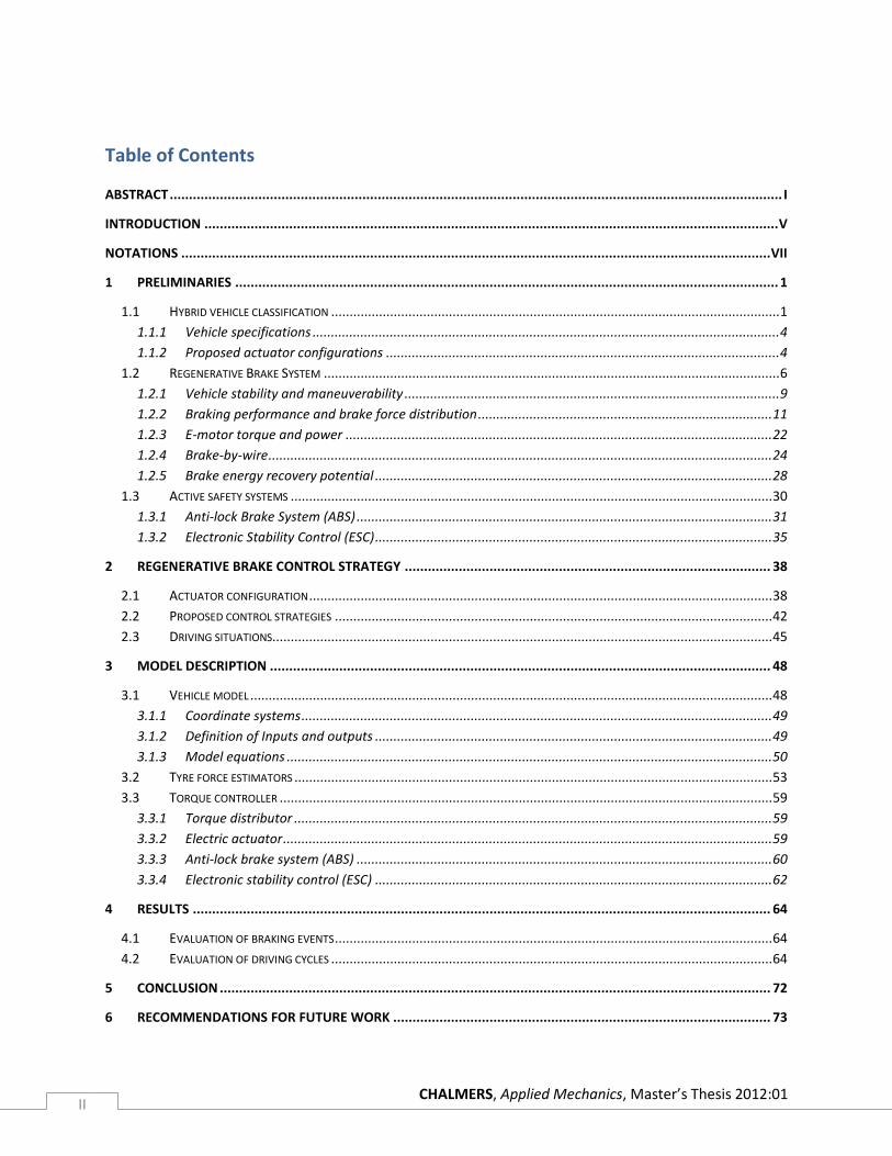
Table of Contents
ABSTRACT ............................................................................................................................................................... I
INTRODUCTION ..................................................................................................................................................... V
NOTATIONS ......................................................................................................................................................... VII
1 PRELIMINARIES ............................................................................................................................................. 1
1.1 HYBRID VEHICLE CLASSIFICATION .......................................................................................................................... 1
1.1.1 Vehicle specifications ............................................................................................................................... 4
1.1.2 Proposed actuator configurations ........................................................................................................... 4
1.2 REGENERATIVE BRAKE SYSTEM ............................................................................................................................ 6
1.2.1 Vehicle stability and maneuverability ...................................................................................................... 9
1.2.2 Braking performance and brake force distribution ................................................................................ 11
1.2.3 E-motor torque and power .................................................................................................................... 22
1.2.4 Brake-by-wire ......................................................................................................................................... 24
1.2.5 Brake energy recovery potential ............................................................................................................ 28
1.3 ACTIVE SAFETY SYSTEMS ................................................................................................................................... 30
1.3.1 Anti-lock Brake System (ABS) ................................................................................................................. 31
1.3.2 Electronic Stability Control (ESC) ............................................................................................................ 35
2 REGENERATIVE BRAKE CONTROL STRATEGY ............................................................................................... 38
2.1 ACTUATOR CONFIGURATION .............................................................................................................................. 38
2.2 PROPOSED CONTROL STRATEGIES ....................................................................................................................... 42
2.3 DRIVING SITUATIONS........................................................................................................................................ 45
3 MODEL DESCRIPTION .................................................................................................................................. 48
3.1 VEHICLE MODEL .............................................................................................................................................. 48
3.1.1 Coordinate systems ................................................................................................................................ 49
3.1.2 Definition of Inputs and outputs ............................................................................................................ 49
3.1.3 Model equations .................................................................................................................................... 50
3.2 TYRE FORCE ESTIMATORS .................................................................................................................................. 53
3.3 TORQUE CONTROLLER ...................................................................................................................................... 59
3.3.1 Torque distributor .................................................................................................................................. 59
3.3.2 Electric actuator ..................................................................................................................................... 59
3.3.3 Anti-lock brake system (ABS) ................................................................................................................. 60
3.3.4 Electronic stability control (ESC) ............................................................................................................ 62
4 RESULTS ...................................................................................................................................................... 64
4.1 EVALUATION OF BRAKING EVENTS ....................................................................................................................... 64
4.2 EVALUATION OF DRIVING CYCLES ........................................................................................................................ 64
5 CONCLUSION ............................................................................................................................................... 72
6 RECOMMENDATIONS FOR FUTURE WORK .................................................................................................. 73
CHALMERS, Applied Mechanics, Master’s Thesis 2012:01 III
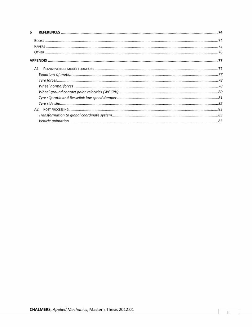
6 REFERENCES ................................................................................................................................................ 74
BOOKS ....................................................................................................................................................................... 74
PAPERS ...................................................................................................................................................................... 75
OTHER ....................................................................................................................................................................... 76
APPENDIX ............................................................................................................................................................ 77
A1 PLANAR VEHICLE MODEL EQUATIONS ....................................................................................................................... 77
Equations of motion ............................................................................................................................................ 77
Tyre forces ........................................................................................................................................................... 78
Wheel normal forces ........................................................................................................................................... 78
Wheel-ground contact point velocities (WGCPV) ............................................................................................... 80
Tyre slip ratio and Besselink low speed damper ................................................................................................. 81
Tyre side slip ........................................................................................................................................................ 82
A2 POST PROCESSING................................................................................................................................................ 83
Transformation to global coordinate system ...................................................................................................... 83
Vehicle animation ............................................................................................................................................... 83

CHALMERS, Applied Mechanics, Master’s Thesis 2012:01 IV
CHALMERS, Applied Mechanics, Master’s Thesis 2012:01 V
INTRODUCTION The attempt to further reduce fuel consumption and CO2 emissions has created a large interest in
hybrid drive train technology. Pioneers on the hybrid market are Japanese carmakers as Toyota and
Honda who are producing hybrid cars since the mid 90s. The focus of the European market has been on
diesel technology but is currently shifting to vehicle electrification. Although not having a hybrid or full
electric vehicle model on the market, Saab has done a lot of research in the field of hybrid drive train
technology.
An important feature of hybrid drive trains is the capability to recover the kinetic energy of the bodies
translating mass that is otherwise dissipated as heat by the friction brakes. Such a system is called a
regenerative brake system (RBS). The majority of current hybrid electric vehicles operate the traction
motor as a generator, providing a brake torque to the wheels. The energy recovery takes place by
transforming this torque into electrical energy via the generator that stores it in an energy storage
system (e.g. battery). Brake energy recovery is limited by two factors. The first is the state of charge
(SOC) of the energy storage system. When the SOC is at an upper charge limit, the RBS does not allow
further recuperation. Second is the insufficient amount of brake torque, provided by the generator, to
reach high vehicle decelerations. Therefore the RBS has to be merged with a friction brake system. As
the name may presume ‘electric vehicle blended braking’ combines (or blends) two brake systems; a
regenerative brake system with a friction brake system. The trade-off is the proper brake force
distribution to minimize braking distance and maintaining a stable traveling direction under varying
environmental conditions, while recuperating a large as possible portion of the brake energy. The
primary requirement of the total brake system is the brake performance, minimizing brake distance in a
stable manner. The distribution of brake torque does not only have an influence on the yaw stability of a
vehicle, but also determines how much energy can be recovered. The aim of the RBS is to retain the
same measure of safety while recovering the largest possible amount of kinetic energy. The thesis aims
to gain a better understanding to what extent a RBS is capable of recovering energy and how it will
affect vehicle stability. The objective is to ‘find a way to control regenerative brake torque, to obtain
maximum energy recovery while maintaining vehicle stability and maneuverability.’ The outcome is a
proposal for control strategies and system limitations for the RBS in different e-motor configurations.
This report starts with a literature review. The different regenerative brake system (RBS) lay-outs and
their main components are analyzed. The conflict between maximum recovery of brake energy, brake
system regulations and control of vehicle motion is graphically illustrated on the brake force distribution
chart. The variability of RBS torque is discussed with the torque and power characteristics of the electric
motor. Heat losses and efficiencies of electrical components and drive line are left out of scope. The two
prominent examples of brake-by-wire systems; Electric Hydraulic Brake (EHB) and Electro Mechanical
Brake (EMB) are described together with the conventional active safety systems. Brake-by-wire is likely
to be used in conjunction with blended brake control. Chapter two motivates the selection of one
electric actuator configuration and the driving situations for which simulations are carried out. It
determines to what extend the control variability is allowed for safe RBS operation. Control of the
electric motor with three different strategies is proposed. Only two of those control strategies are
simulated due to shortage of time. Chapter three covers the model developed in MATLAB Simulink and

CHALMERS, Applied Mechanics, Master’s Thesis 2012:01 VI
gives a description of the tyre force estimators by means of look-up tables. Optimized recovery is
measured on a standardized driving cycle (NEDC) and is presented in chapter four. The yaw stability is
proved by simulated braking events, which are critical for yaw stability. The quantified energy recovery
on the driving cycles is an addition to the project carried out in August 2011 that presented a qualitative
result of regenerative braking.
CHALMERS, Applied Mechanics, Master’s Thesis 2012:01 VII
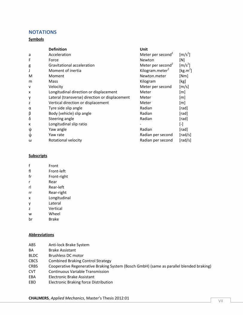
NOTATIONS Symbols
Definition Unit a Acceleration Meter per second2 [m/s2] F Force Newton [N] g Gravitational acceleration Meter per second2 [m/s2] J Moment of inertia Kilogram.meter2 [kg.m2] M Moment Newton.meter [Nm] m Mass Kilogram [kg] v Velocity Meter per second [m/s] x Longitudinal direction or displacement Meter [m] y Lateral (transverse) direction or displacement Meter [m] z Vertical direction or displacement Meter [m] α Tyre side slip angle Radian [rad] β Body (vehicle) slip angle Radian [rad] δ Steering angle Radian [rad] κ Longitudinal slip ratio - [-] ψ Yaw angle Radian [rad]
ψ Yaw rate Radian per second [rad/s] ω Rotational velocity Radian per second [rad/s]
Subscripts
f Front fl Front-left fr Front-right r Rear rl Rear-left rr Rear-right x Longitudinal y Lateral z Vertical w Wheel br Brake
Abbreviations
ABS Anti-lock Brake System BA Brake Assistant BLDC Brushless DC motor CBCS Combined Braking Control Strategy CRBS Cooperative Regenerative Braking System (Bosch GmbH) (same as parallel blended braking) CVT Continuous Variable Transmission EBA Electronic Brake Assistant EBD Electronic Braking force Distribution
CHALMERS, Applied Mechanics, Master’s Thesis 2012:01 VIII
ECU Electronic Control Unit EDIB Electric Driven Intelligent Brake (Nissan) EHB Electro-Hydraulic Braking EMB Electro-Mechanical Braking ESC Electronic Stability Control ESP Electronic Stability Program HBA Hydraulic Brake Assistant HCU Hybrid system Control Unit HECU Hydraulic-Electronic Control Unit HEV Hybrid Electric Vehicle LTCS Logic Threshold Control Strategy MBA Mechanical Brake Assistant RBS Regenerative Brake System SRBS Superimposed Regenerative Braking System (same as series braking) TCS Traction Control System TCU Traction Control Unit ZEV Zero Emission Vehicle


CHALMERS, Applied Mechanics, Master’s Thesis 2012:01 1
1 Preliminaries
1.1 Hybrid vehicle classification
A hybrid vehicle is a vehicle with two (or multiple) power trains. The drive train of a vehicle is the
composition of all the power trains. A hybrid vehicle with an electric power train is called a hybrid
electric vehicle (HEV).
The principle of hybrid vehicles dates back to the beginning of the 20th century, were both the series-
and parallel hybrid were introduced. In these first hybrid vehicles an electric machine was used to aid
the early internal combustion engines that were too weak to propel a vehicle by their own. The hybrid
electric vehicles disappeared, after few years, when specific power output of the internal combustion
engines improved. There is no evidence of brake energy recovery by a regenerative brake system,
although these early designs used electric braking by short circuiting or by placing a resistance in the
armature of the electric motor [1]. The greatest difficulty was the control of the electric motor with
resistors and mechanical switches, because power electronics became available in 1960s. In the late 20th
century the concept of vehicle electrification was re-introduced to reduce emissions and improve fuel
economy. The main reasons for the poor fuel economy of Internal Combustion Engine (ICE) vehicles are;
The ICE is most efficient in a small range, usually maximum torque in the mid range of rotational
speed. Real operation requirements for urban cycles do not match the sweet spot on the brake
specific fuel consumption chart of an ICE.
The kinetic energy of the translating body, initially build up by the ICE, is dissipated into heat by
the friction brakes during braking. This ‘wasted’ energy becomes significant when operating in
urban cycles.
Low efficiency of non-geared parts of transmission (i.e. clutches, torque converters, CVTs, etc) in
current automobiles in stop-and-go driving patterns.
A fully electric vehicle (EV) has zero emission and high energy efficiency while driving. However, there is
a weight penalty for the battery pack implying that the energy density of batteries is far less than that of
fossil fuels. Beside that, the efficiency from ‘well-to-wheel’ is not as significant as the efficiency
improvement on vehicle level. The hybrid electric vehicle merges the advantages of a conventional and
electric power train by the use of both. To allow kinetic energy recuperation the electric power train in a
hybrid drive should allow energy to flow bidirectionally. Control issues of hybrid drives arise when
switching between different operation modes (e.g. electric propulsion, hybrid propulsion, regeneration).
Fast and smooth change from EV to HEV mode, good shifting quality and good drivability during
generative braking, must be assured by the Hybrid Control Unit (HCU).
The hybrid vehicles can be roughly classified by the connection between power train components that
define the flow of energy. In 2000 some hybrid drive trains, like the Toyota Prius, where introduced that
could not be classified as a series nor parallel hybrid. Hence, on the current market there is made a
distinction between four types of hybrid drive lines; series hybrid, parallel hybrid, series-parallel hybrid
CHALMERS, Applied Mechanics, Master’s Thesis 2012:01 2
and complex hybrid [1]. From a scientific point of view these classifications are vaguely defined. M.
Eshani, Y. Gao and A. Emadi [1], propose to refer to the power coupling, that connects the power trains
in the drive train;
“Adding two powers together or splitting one power into two at the power merging point always occurs
with the same power type, that is electrical or mechanical, not electrical and mechanical. So perhaps a
more accurate definition of HEV architecture may be to take the power coupling or decoupling features
such as an electrical coupling drive train, a mechanical coupling drive train, and a mechanical-electrical
coupling drive train.”
A series hybrid drive train has an electrical coupling, which adds the electrical powers coming from the
ICE generator and from the batteries. The ICE is the primary power source, which can be independently
operated in the most efficient region, because there is no mechanical connection to the driveshaft. The
batteries function as energy buffer. The series hybrid is from origin based on an EV on which an extra
power source (ICE) is added to extend the limited range, caused by the poor energy density of the
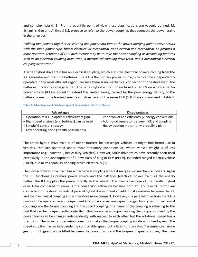
battery. Some of the leading benefits and drawbacks of the series HEV (SHEV) are summarized in table 1.
Table 1: Advantages and disadvantages of series hybrid electric vehicles
Advantages Disadvantages
+ Operation of ICE in optimal efficiency region + High speed engines (e.g. turbines) can be used + Simple(r) control strategy + Low operating noise (stealth possibilities)
- Poor conversion efficiency (2 energy conversions) - Additional generator between ICE and coupling - Heavy traction motor (only propelling plant)
The series hybrid drive train is of minor interest for passenger vehicles. It might find better use in
vehicles, that are operated under more stationary conditions or, where vehicle weight is of less
importance (e.g. industrial-, heavy duty vehicles). However, SHEV drive trains have recently been used
extensively in the development of a new class of plug-in HEV (PHEV), extended ranged electric vehicle
(EREV), due to its capability of being driven electrically [3].
The parallel hybrid drive train has a mechanical coupling where it merges two mechanical powers. Again
the ICE functions as primary power source and the batteries (electrical power train) as the energy
buffer. The ICE supplies the power directly to the wheels. The main advantage of the parallel hybrid
drive train compared to series is the conversion efficiency because both ICE and electric motor are
connected to the driven wheels. A parallel hybrid doesn’t need an additional generator between the ICE
and the mechanical coupling and is therefore more compact. However, in a parallel drive train the ICE is
unable to be operated in an independent (stationary or narrow) speed range. Two types of mechanical
couplings are the torque coupling and the speed coupling. The name of the coupling is referring to the
unit that can be independently controlled. That means, in a torque coupling the torque supplied by the
power trains can be changed independently with respect to each other but the rotational speed has a
fixed ratio. The power conservation constraint makes the torque coupling rotate with fixed speed. The
speed coupling has an independently controllable speed but a fixed torque ratio. Transmissions (single
gear or multi gear) can be fitted between the power trains and the torque- or speed coupling. The main
CHALMERS, Applied Mechanics, Master’s Thesis 2012:01 3
advantage of the hybrid drive train with speed coupling is that the speed of the two power plants can be
decoupled from vehicle speed. This is an important advantage for power plants, where operating
efficiency is more sensitive to speed rather than torque. Benefits and drawbacks of the parallel HEV are
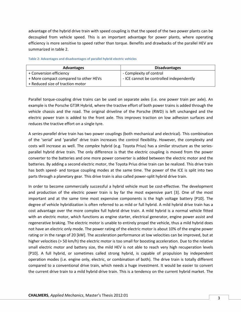
summarized in table 2.
Table 2: Advantages and disadvantages of parallel hybrid electric vehicles
Advantages Disadvantages
+ Conversion efficiency + More compact compared to other HEVs + Reduced size of traction motor
- Complexity of control - ICE cannot be controlled independently
Parallel torque-coupling drive trains can be used on separate axles (i.e. one power train per axle). An
example is the Porsche GT3R Hybrid, where the tractive effort of both power trains is added through the
vehicle chassis and the road. The original driveline of the Porsche (RWD) is left unchanged and the
electric power train is added to the front axle. This improves traction on low adhesion surfaces and
reduces the tractive effort on a single tyre.
A series-parallel drive train has two power couplings (both mechanical and electrical). This combination
of the ‘serial’ and ‘parallel’ drive train increases the control flexibility. However, the complexity and
costs will increase as well. The complex hybrid (e.g. Toyota Prius) has a similar structure as the series-
parallel hybrid drive train. The only difference is that the electric coupling is moved from the power
converter to the batteries and one more power converter is added between the electric motor and the
batteries. By adding a second electric motor, the Toyota Prius drive train can be realized. This drive train
has both speed- and torque coupling modes at the same time. The power of the ICE is split into two
parts through a planetary gear. This drive train is also called power-split hybrid drive train.
In order to become commercially successful a hybrid vehicle must be cost-effective. The development
and production of the electric power train is by far the most expensive part [3]. One of the most
important and at the same time most expensive components is the high voltage battery [P10]. The
degree of vehicle hybridization is often referred to as mild or full hybrid. A mild hybrid drive train has a
cost advantage over the more complex full hybrid drive train. A mild hybrid is a normal vehicle fitted
with an electric motor, which functions as engine starter, electrical generator, engine power assist and
regenerative braking. The electric motor is unable to entirely propel the vehicle, thus a mild hybrid does
not have an electric only mode. The power rating of the electric motor is about 10% of the engine power
rating or in the range of 20 [kW]. The acceleration performance at low velocities can be improved, but at
higher velocities (> 50 km/h) the electric motor is too small for boosting acceleration. Due to the relative
small electric motor and battery size, the mild HEV is not able to reach very high recuperation levels
[P10]. A full hybrid, or sometimes called strong hybrid, is capable of propulsion by independent
operation modes (i.e. engine only, electric, or combination of both). The drive train is totally different
compared to a conventional drive train, which needs a huge investment. It would be easier to convert
the current drive train to a mild hybrid drive train. This is a tendency on the current hybrid market. The
CHALMERS, Applied Mechanics, Master’s Thesis 2012:01 4
chassis and suspension systems used in today’s early hybrid vehicles are mostly adaptations of standard
systems and do not include any revolutionary changes or new solutions [3].
1.1.1 Vehicle specifications
Identical vehicle dimensions and masses will be used for all actuator configurations (paragraph 1.1.2), to
make them better comparable with respect to their vehicle dynamic performance. That means added
weight of electrical components and variation of center of gravity position will not be taken into
account. The position of the vehicle mass center is an important variable in determining the brake force
distribution. Deviations in vehicle weight distribution, due to different driveline components, can be in
favor of one driveline. The objectives of this study are maximizing and correctly distributing the
regenerative brake torque among the wheels and consider the effect on vehicle stability and
maneuverability. Table 3 summarizes the vehicle dimensions and parameters used, throughout the
study and presented in this report. The MATLAB Simulink models are programmed in terms of these
variables and can be altered by changing the vehicle specifications in the model initialization file.
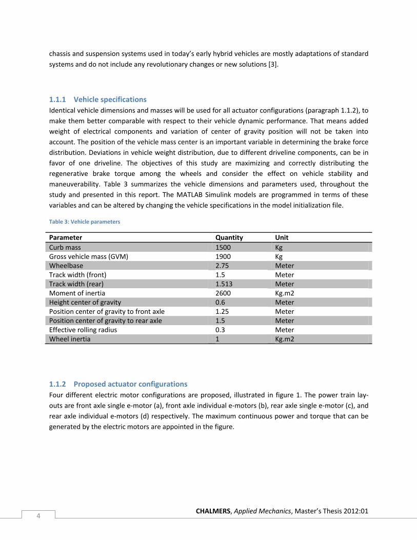
Table 3: Vehicle parameters
Parameter Quantity Unit
Curb mass 1500 Kg Gross vehicle mass (GVM) 1900 Kg Wheelbase 2.75 Meter Track width (front) 1.5 Meter Track width (rear) 1.513 Meter Moment of inertia 2600 Kg.m2 Height center of gravity 0.6 Meter Position center of gravity to front axle 1.25 Meter Position center of gravity to rear axle 1.5 Meter Effective rolling radius 0.3 Meter Wheel inertia 1 Kg.m2
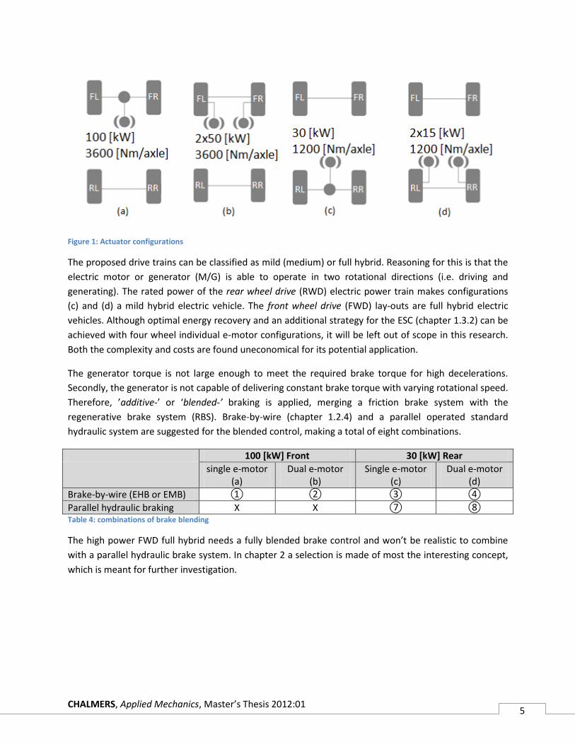
1.1.2 Proposed actuator configurations
Four different electric motor configurations are proposed, illustrated in figure 1. The power train lay-
outs are front axle single e-motor (a), front axle individual e-motors (b), rear axle single e-motor (c), and
rear axle individual e-motors (d) respectively. The maximum continuous power and torque that can be
generated by the electric motors are appointed in the figure.
CHALMERS, Applied Mechanics, Master’s Thesis 2012:01 5
Figure 1: Actuator configurations
The proposed drive trains can be classified as mild (medium) or full hybrid. Reasoning for this is that the
electric motor or generator (M/G) is able to operate in two rotational directions (i.e. driving and
generating). The rated power of the rear wheel drive (RWD) electric power train makes configurations
(c) and (d) a mild hybrid electric vehicle. The front wheel drive (FWD) lay-outs are full hybrid electric
vehicles. Although optimal energy recovery and an additional strategy for the ESC (chapter 1.3.2) can be
achieved with four wheel individual e-motor configurations, it will be left out of scope in this research.
Both the complexity and costs are found uneconomical for its potential application.
The generator torque is not large enough to meet the required brake torque for high decelerations.
Secondly, the generator is not capable of delivering constant brake torque with varying rotational speed.
Therefore, ’additive-’ or ‘blended-’ braking is applied, merging a friction brake system with the
regenerative brake system (RBS). Brake-by-wire (chapter 1.2.4) and a parallel operated standard
hydraulic system are suggested for the blended control, making a total of eight combinations.
100 [kW] Front 30 [kW] Rear
single e-motor (a)
Dual e-motor (b)
Single e-motor (c)
Dual e-motor (d)
Brake-by-wire (EHB or EMB) ① ② ③ ④
Parallel hydraulic braking X X ⑦ ⑧ Table 4: combinations of brake blending
The high power FWD full hybrid needs a fully blended brake control and won’t be realistic to combine
with a parallel hydraulic brake system. In chapter 2 a selection is made of most the interesting concept,
which is meant for further investigation.
CHALMERS, Applied Mechanics, Master’s Thesis 2012:01 6
1.2 Regenerative Brake System
A regenerative brake system (RBS) converts the kinetic energy, caused by the deceleration of the vehicle
body, into another type of energy (e.g. electric, rotational kinetic) instead of dissipating it as heat
through friction brakes. Brake energy recuperation is an important feature of electrified vehicles and will
become increasingly important in future vehicles. In electric vehicles (EV), RBS operates as range
extender and in hybrid electric vehicles (HEV) RBS significantly reduces emissions.
Hano and Hakiai [P10] present a comparison of fuel savings for a luxury SUV on the New European
Driving Cycle (NEDC). Parallel hybridization without energy recuperation promises a fuel reduction of
approximately 20% in comparison with a similar sized non-hybrid vehicle. Adding brake energy recovery
saves an additional 6% on fuel consumption. However, it must be emphasized that the efficiency gain,
due to energy recovery, is considerably higher in urban driving than normal use on highways. This is
caused by frequent moderate braking events in urban areas, which allow full regenerative brake
exploitation [P16].
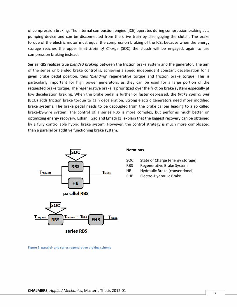
As mentioned in previous paragraph the electric motor is unable to provide all the brake torque
necessary for large decelerations. If regenerative brake torque is only applied to one axle, stability and
maneuverability issues can occur (paragraph 1.2.1). Therefore, regenerative braking is operated in
conjunction with a friction brake system. A frequently used name for regenerative braking is ‘hybrid’
braking, as it obtains the total brake torque from two different sources (figure 2). Two groups of
regenerative brake systems (RBS) can be roughly distinguished named parallel RBS and series RBS, or
“without torque blending” and “with torque blending” [P10]. Within the EVBB project the names Add-on
(additive) braking and blended braking are used to denote parallel and series RBS. Bosch uses other
terminology for their brake system development; Superimposed Regenerative Braking System (SRBS)
and Cooperative Regenerative Braking System (CRBS), corresponding with parallel- and serial RBS,
respectively. In both braking systems a portion of the kinetic energy is recuperated by the RBS and the
remainder is dissipated by the friction brakes. Just like vehicle propulsion the braking can be divided in
three different working stages;
Generator (electric) braking
Hybrid braking (Add-on or blended)
Friction braking
A parallel RBS works ‘in parallel’ with a friction brake system (figure 2), meaning that the conventional
brake system layout remains virtually unchanged. The brake pedal is mechanically coupled with the
brake caliper and the brake pressure is proportional to the pedal travel and force. The electric motor (in
generator mode) will add an additional brake torque. The driver’s brake pedal feel must be the same as
a conventional brake system. That means, with the same pedal input (i.e. travel and force), the total
brake force of the parallel RBS should reach the same deceleration as the conventional system [P6].
Therefore, the brake torque added by the generator can’t be very large and the recuperation potential is
limited. A big advantage of parallel RBS is that there is no requirement for brake-by-wire (chapter 1.2.4).
This means the brake control will be less sophisticated and the brake system has a high reliability.
Parallel RBS is most commonly used in mild hybrids. The parallel braking system can be applied instead
CHALMERS, Applied Mechanics, Master’s Thesis 2012:01 7
of compression braking. The internal combustion engine (ICE) operates during compression braking as a
pumping device and can be disconnected from the drive train by disengaging the clutch. The brake
torque of the electric motor must equal the compression braking of the ICE, because when the energy
storage reaches the upper limit State of Charge (SOC) the clutch will be engaged, again to use
compression braking instead.
Series RBS realizes true blended braking between the friction brake system and the generator. The aim
of the series or blended brake control is, achieving a speed independent constant deceleration for a
given brake pedal position, thus ‘blending’ regenerative torque and friction brake torque. This is
particularly important for high power generators, as they can be used for a large portion of the
requested brake torque. The regenerative brake is prioritized over the friction brake system especially at
low deceleration braking. When the brake pedal is further or faster depressed, the brake control unit
(BCU) adds friction brake torque to gain deceleration. Strong electric generators need more modified
brake systems. The brake pedal needs to be decoupled from the brake caliper leading to a so called
brake-by-wire system. The control of a series RBS is more complex, but performs much better on
optimizing energy recovery. Eshani, Gao and Emadi [1] explain that the biggest recovery can be obtained
by a fully controllable hybrid brake system. However, the control strategy is much more complicated
than a parallel or additive functioning brake system.
Notations SOC State of Charge (energy storage) RBS Regenerative Brake System HB Hydraulic Brake (conventional) EHB Electro-Hydraulic Brake
Figure 2: parallel- and series regenerative braking scheme
CHALMERS, Applied Mechanics, Master’s Thesis 2012:01 8
Independent of the RBS type, these are the main system (brake torque) limitations:
The brake torque is not large enough to meet the requested brake torque during intensive
braking. Power dissipated by a front friction brake can be above 100 [kW].
The electric motor is unable to deliver a constant brake torque in the upper speed range. This
means that the regenerative brake torque is speed dependent while the brake torque request is
not.
At speeds around zero the brake torque of the electric motor drops to zero, due to low motor
electromotive force.
At stand-still friction brakes are better to hold vehicle (parking or holding assist).
Fail-safe function. In case the vehicle electronics malfunction the vehicle should still be able to
come to a standstill, meaning a secondary brake system will be necessary.
RBS availability is limited by the charging condition of the energy storage system.
By vehicle stability under critical driving (low friction or split-µ surfaces).
In case a battery is used as energy storage system, the RBS is not allowed to charge the battery when
the State of Charge (SOC) is at the upper limit, to prevent overcharging. The internal resistance of the
battery rises exponentially above a SOC of approximately 80% but is relatively constant in moderate
charge range [P2]. This 80% SOC is often taken as the upper threshold of battery charge in regenerative
braking control. When a parallel RBS is used a, gradual ramp down of regenerative brake torque is
required. This will give the driver time to react on the loss of regenerative brake torque, by applying
more pedal force and thereby increasing the hydraulic brake torque instead. A series or blended control
will substitute the loss of regenerative torque with the friction brake torque. The regenerative efficiency
is the portion of brake energy, which can be recuperated by a RBS.
For micro HEVs and mild HEVs with small generator power, the available regenerative brake
deceleration is relatively small (e.g. < 1.0 m/s2). In such vehicles, the RBS may be used without blending
control. This means, the conventional hydraulic braking system with standard vacuum booster does not
need to be changed [P10].
CHALMERS, Applied Mechanics, Master’s Thesis 2012:01 9
1.2.1 Vehicle stability and maneuverability
The behavior of a driver-vehicle system is called handling. B. Heissing & M. Ersoy [3] define handling as;
“the vehicles reaction, defined by its motions, to both driver’s actions and disturbances which act on the
vehicle during vehicle movement”. Disturbances might be thought of as aerodynamic influences, road
adhesion (grip), etc. Nowadays one can also think of including the vehicles reaction to the ‘virtual
driver’. These are the (electronic) systems that have a similar request as the (biological) driver (e.g.
functions as collision avoidance). Tuning of a vehicle’s braking behavior, is based on the evaluation of
the braking system on the dynamic effects of deceleration forces on the vehicle motion [3].
During cornering the lateral acceleration creates an external force called ‘centrifugal force’ connected to
the center of gravity and pointing in outwards direction of a corner. This force is used to achieve
equilibrium of the vehicle system so it can be treated as a (quasi) static situation. When the lateral (or
side) peak force on one of the axles is reached (figure 4) the gradient of the force becomes negative and
the side slip angle (alpha) increases rapidly.
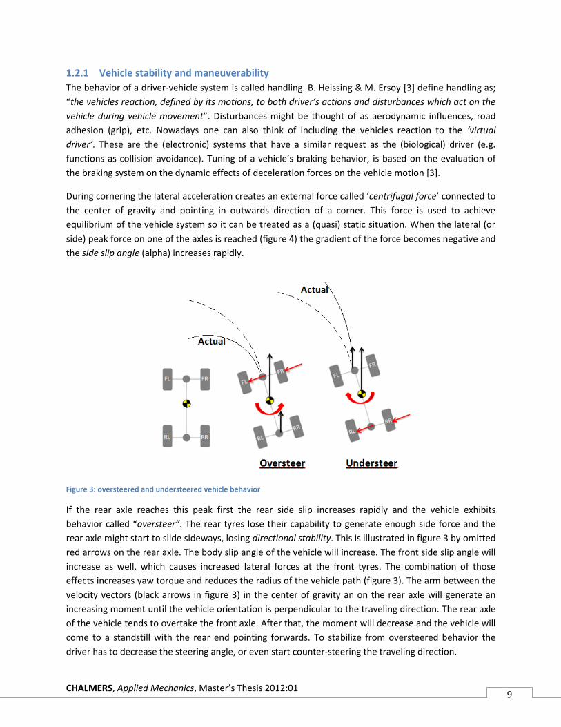
Figure 3: oversteered and understeered vehicle behavior
If the rear axle reaches this peak first the rear side slip increases rapidly and the vehicle exhibits
behavior called “oversteer”. The rear tyres lose their capability to generate enough side force and the
rear axle might start to slide sideways, losing directional stability. This is illustrated in figure 3 by omitted
red arrows on the rear axle. The body slip angle of the vehicle will increase. The front side slip angle will
increase as well, which causes increased lateral forces at the front tyres. The combination of those
effects increases yaw torque and reduces the radius of the vehicle path (figure 3). The arm between the
velocity vectors (black arrows in figure 3) in the center of gravity an on the rear axle will generate an
increasing moment until the vehicle orientation is perpendicular to the traveling direction. The rear axle
of the vehicle tends to overtake the front axle. After that, the moment will decrease and the vehicle will
come to a standstill with the rear end pointing forwards. To stabilize from oversteered behavior the
driver has to decrease the steering angle, or even start counter-steering the traveling direction.
CHALMERS, Applied Mechanics, Master’s Thesis 2012:01 10
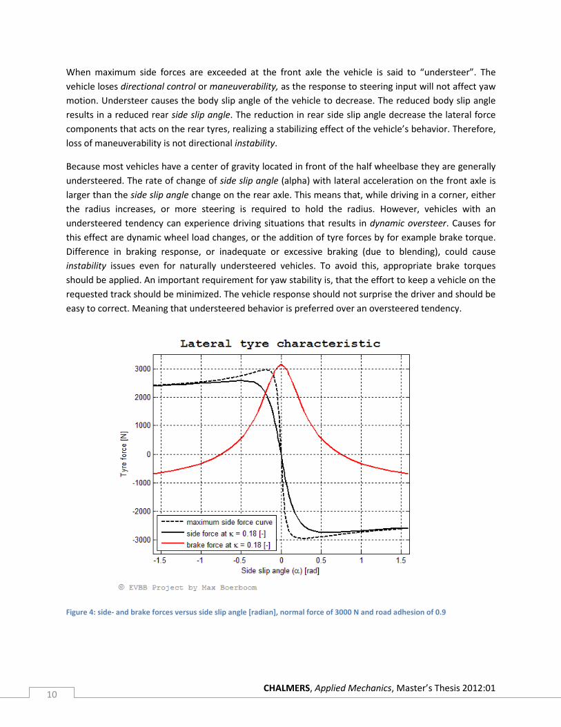
When maximum side forces are exceeded at the front axle the vehicle is said to “understeer”. The
vehicle loses directional control or maneuverability, as the response to steering input will not affect yaw
motion. Understeer causes the body slip angle of the vehicle to decrease. The reduced body slip angle
results in a reduced rear side slip angle. The reduction in rear side slip angle decrease the lateral force
components that acts on the rear tyres, realizing a stabilizing effect of the vehicle’s behavior. Therefore,
loss of maneuverability is not directional instability.
Because most vehicles have a center of gravity located in front of the half wheelbase they are generally
understeered. The rate of change of side slip angle (alpha) with lateral acceleration on the front axle is
larger than the side slip angle change on the rear axle. This means that, while driving in a corner, either
the radius increases, or more steering is required to hold the radius. However, vehicles with an
understeered tendency can experience driving situations that results in dynamic oversteer. Causes for
this effect are dynamic wheel load changes, or the addition of tyre forces by for example brake torque.
Difference in braking response, or inadequate or excessive braking (due to blending), could cause
instability issues even for naturally understeered vehicles. To avoid this, appropriate brake torques
should be applied. An important requirement for yaw stability is, that the effort to keep a vehicle on the
requested track should be minimized. The vehicle response should not surprise the driver and should be
easy to correct. Meaning that understeered behavior is preferred over an oversteered tendency.
Figure 4: side- and brake forces versus side slip angle [radian], normal force of 3000 N and road adhesion of 0.9
CHALMERS, Applied Mechanics, Master’s Thesis 2012:01 11
1.2.2 Braking performance and brake force distribution
The function of the braking system is the deceleration of the vehicle in a quick and safe manner, while
the travel direction remains controllable. This paragraph describes the front-to-rear brake force
distribution for pure longitudinal deceleration. The working area of the hybrid braking system and the
flexibility of brake proportionality is considered. The ECE regulation No. 13H that determine the working
area of brake force distribution will be explained.
The brake force diagram is fundamental to the design of a brake system and can be drawn using only
geometric vehicle data and weight distribution [3]. The distribution of the braking forces between the
front and rear axle have an influence on:
Stopping distance. The shortest distance is reached with optimal utilization of adhesion.
Vehicle directional control during braking. Over-braking the front axle leads to poor steer
response.
Vehicle stability during braking. Over-braking the rear axle leads to loss of stability.
Durability and thermal loading of brakes. The wear reduction due regenerative braking will have
the largest impact on the strongest braked axle.
A Regenerative braking system does not only have to meet the brake force requirements, but also has to
recuperate a large as possible energy portion. The hybrid braking system uses two sources of braking
torque. Criteria for the design are:
Large enough braking force for vehicle deceleration
Appropriate distribution of braking forces to ensure the stability of the vehicle
Recuperate as much energy as possible, assuring the above criteria.
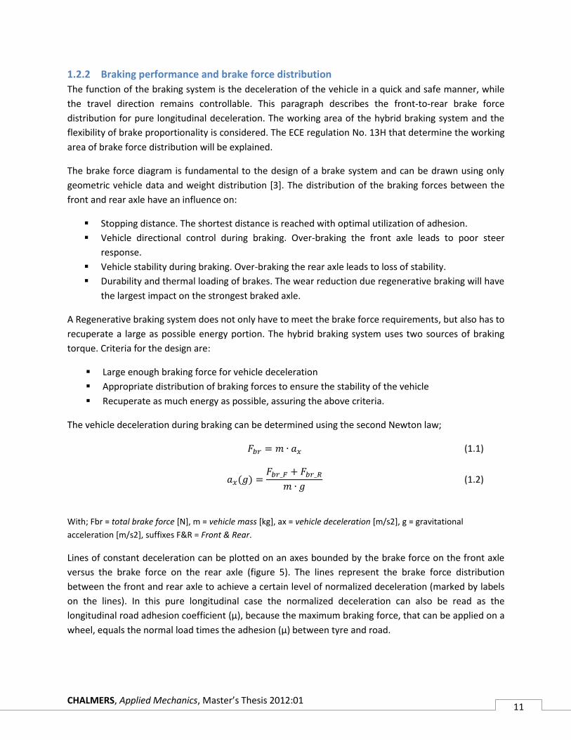
The vehicle deceleration during braking can be determined using the second Newton law;
(1.1)
(1.2)
With; Fbr = total brake force [N], m = vehicle mass [kg], ax = vehicle deceleration [m/s2], g = gravitational
acceleration [m/s2], suffixes F&R = Front & Rear.
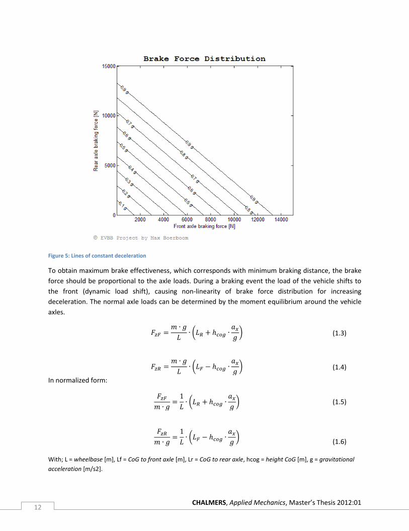
Lines of constant deceleration can be plotted on an axes bounded by the brake force on the front axle
versus the brake force on the rear axle (figure 5). The lines represent the brake force distribution
between the front and rear axle to achieve a certain level of normalized deceleration (marked by labels
on the lines). In this pure longitudinal case the normalized deceleration can also be read as the
longitudinal road adhesion coefficient (µ), because the maximum braking force, that can be applied on a
wheel, equals the normal load times the adhesion (µ) between tyre and road.
CHALMERS, Applied Mechanics, Master’s Thesis 2012:01 12
Figure 5: Lines of constant deceleration
To obtain maximum brake effectiveness, which corresponds with minimum braking distance, the brake
force should be proportional to the axle loads. During a braking event the load of the vehicle shifts to
the front (dynamic load shift), causing non-linearity of brake force distribution for increasing
deceleration. The normal axle loads can be determined by the moment equilibrium around the vehicle
axles.
(1.3)
(1.4)
In normalized form:
(1.5)
(1.6)
With; L = wheelbase [m], Lf = CoG to front axle [m], Lr = CoG to rear axle, hcog = height CoG [m], g = gravitational
acceleration [m/s2].
CHALMERS, Applied Mechanics, Master’s Thesis 2012:01 13
The (ideal) brake force proportionality factor front-to-rear is then given by the ratio of the normal loads:
(1.7)
Where the front and rear brake forces can be written as;
(1.8)
If equation 1.2 is expanded by equation 1.8, the rear portion of the brake force in ideal case becomes:
(1.9)
The same way the front portion of the braking force becomes:
(1.10)
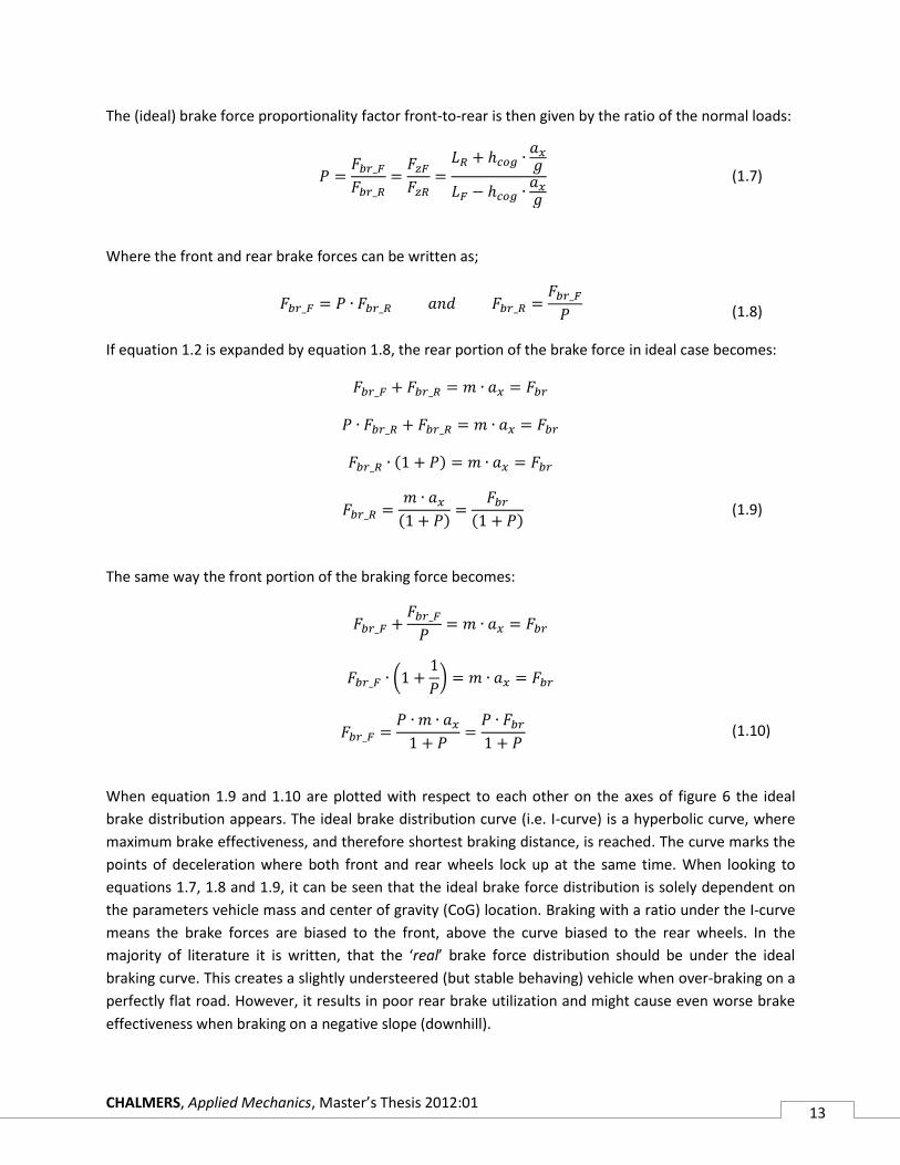
When equation 1.9 and 1.10 are plotted with respect to each other on the axes of figure 6 the ideal
brake distribution appears. The ideal brake distribution curve (i.e. I-curve) is a hyperbolic curve, where
maximum brake effectiveness, and therefore shortest braking distance, is reached. The curve marks the
points of deceleration where both front and rear wheels lock up at the same time. When looking to
equations 1.7, 1.8 and 1.9, it can be seen that the ideal brake force distribution is solely dependent on
the parameters vehicle mass and center of gravity (CoG) location. Braking with a ratio under the I-curve
means the brake forces are biased to the front, above the curve biased to the rear wheels. In the
majority of literature it is written, that the ‘real’ brake force distribution should be under the ideal
braking curve. This creates a slightly understeered (but stable behaving) vehicle when over-braking on a
perfectly flat road. However, it results in poor rear brake utilization and might cause even worse brake
effectiveness when braking on a negative slope (downhill).
CHALMERS, Applied Mechanics, Master’s Thesis 2012:01 14
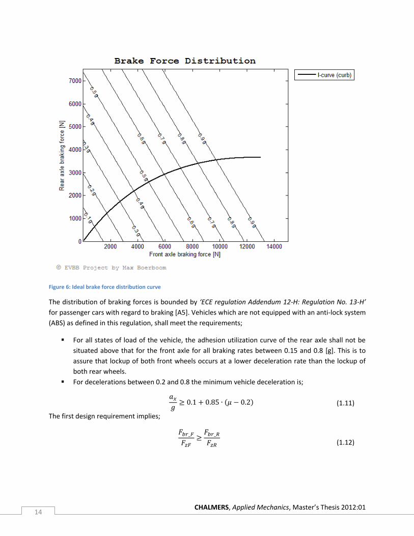
Figure 6: Ideal brake force distribution curve
The distribution of braking forces is bounded by ‘ECE regulation Addendum 12-H: Regulation No. 13-H’
for passenger cars with regard to braking [A5]. Vehicles which are not equipped with an anti-lock system
(ABS) as defined in this regulation, shall meet the requirements;
For all states of load of the vehicle, the adhesion utilization curve of the rear axle shall not be
situated above that for the front axle for all braking rates between 0.15 and 0.8 [g]. This is to
assure that lockup of both front wheels occurs at a lower deceleration rate than the lockup of
both rear wheels.
For decelerations between 0.2 and 0.8 the minimum vehicle deceleration is;
(1.11)
The first design requirement implies;
(1.12)
CHALMERS, Applied Mechanics, Master’s Thesis 2012:01 15
Meaning the normalized front portion is larger or equal to the normalized rear portion, because the
ideal brake force distribution (I-curve) is expressed by;
(1.13)
The second ECE requirement states the minimum vehicle deceleration, that must be achieved by the
rear wheels, when front wheels are locked (equation 1.11). This is the total brake force related to the
adhesion coefficient (µ). The rear brake force becomes;
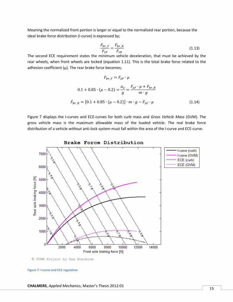
(1.14)
Figure 7 displays the I-curves and ECE-curves for both curb mass and Gross Vehicle Mass (GVM). The
gross vehicle mass is the maximum allowable mass of the loaded vehicle. The real brake force
distribution of a vehicle without anti-lock system must fall within the area of the I-curve and ECE-curve.
Figure 7: I-curve and ECE regulation

CHALMERS, Applied Mechanics, Master’s Thesis 2012:01 16
When considering that, at all times, lockup of the rear wheels must be avoided, it becomes clear that
the I-curve for an empty (curb mass) vehicle is critical. Before the introduction of the anti-lock systems
with hydraulic modulators the brake system was designed to have a fixed brake portion between the
front and rear axle. To prevent rear lock-up and meet the ECE regulations a conservative approach was
taken, leading to front always locking up first until the assumed maximum adhesion coefficient of 0.8 is
exceeded. When a brake system and components are used for platforming1 the system is calibrated for
the worst case scenario leading to poor rear brake utilization of the heavier vehicle lay-outs. The
proportionality is dependent on the brake system design, not on the dimensions and parameters of the
vehicle [1]. When brake proportionality is introduced;
(1.15)
(1.16)
The linear brake curve intersects with the I-curve for one value of deceleration or adhesion coefficient. If
the normalized deceleration in the formula of the proportionality factor (equation 1.7) is replaced by the
adhesion coefficient the linear proportional factor can be determined.
(1.17)
(1.18)
(1.19)
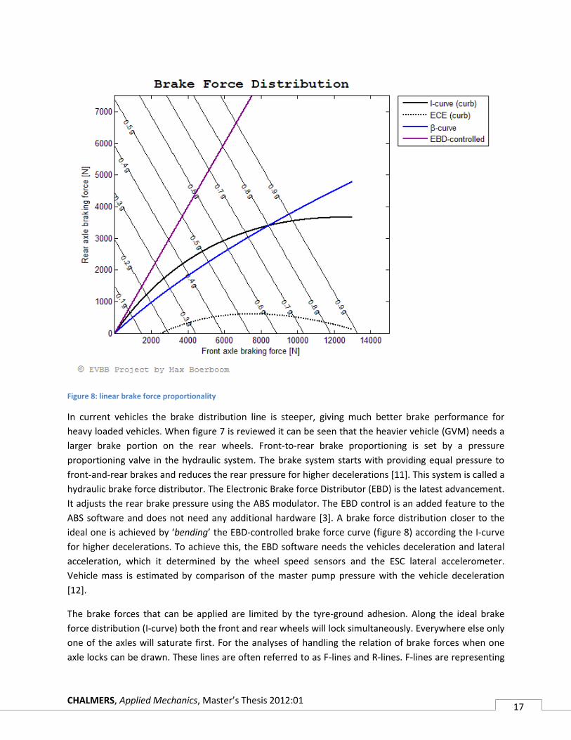
Figure 8 illustrates the linear brake curve for vehicle curb weight, intersecting the I-curve at 0.8 [g]. All
road surfaces with an adhesive coefficient smaller 0.8 result in front wheel locking first. Road adhesive
coefficients larger than the line intersection will generate rear lockup.
1 Platforming is the exchange of vehicle components between different types of vehicles (e.g. one entire braking
system can be used on a class of similar vehicles).
CHALMERS, Applied Mechanics, Master’s Thesis 2012:01 17
Figure 8: linear brake force proportionality
In current vehicles the brake distribution line is steeper, giving much better brake performance for
heavy loaded vehicles. When figure 7 is reviewed it can be seen that the heavier vehicle (GVM) needs a
larger brake portion on the rear wheels. Front-to-rear brake proportioning is set by a pressure
proportioning valve in the hydraulic system. The brake system starts with providing equal pressure to
front-and-rear brakes and reduces the rear pressure for higher decelerations [11]. This system is called a
hydraulic brake force distributor. The Electronic Brake force Distributor (EBD) is the latest advancement.
It adjusts the rear brake pressure using the ABS modulator. The EBD control is an added feature to the
ABS software and does not need any additional hardware [3]. A brake force distribution closer to the
ideal one is achieved by ‘bending’ the EBD-controlled brake force curve (figure 8) according the I-curve
for higher decelerations. To achieve this, the EBD software needs the vehicles deceleration and lateral
acceleration, which it determined by the wheel speed sensors and the ESC lateral accelerometer.
Vehicle mass is estimated by comparison of the master pump pressure with the vehicle deceleration
[12].
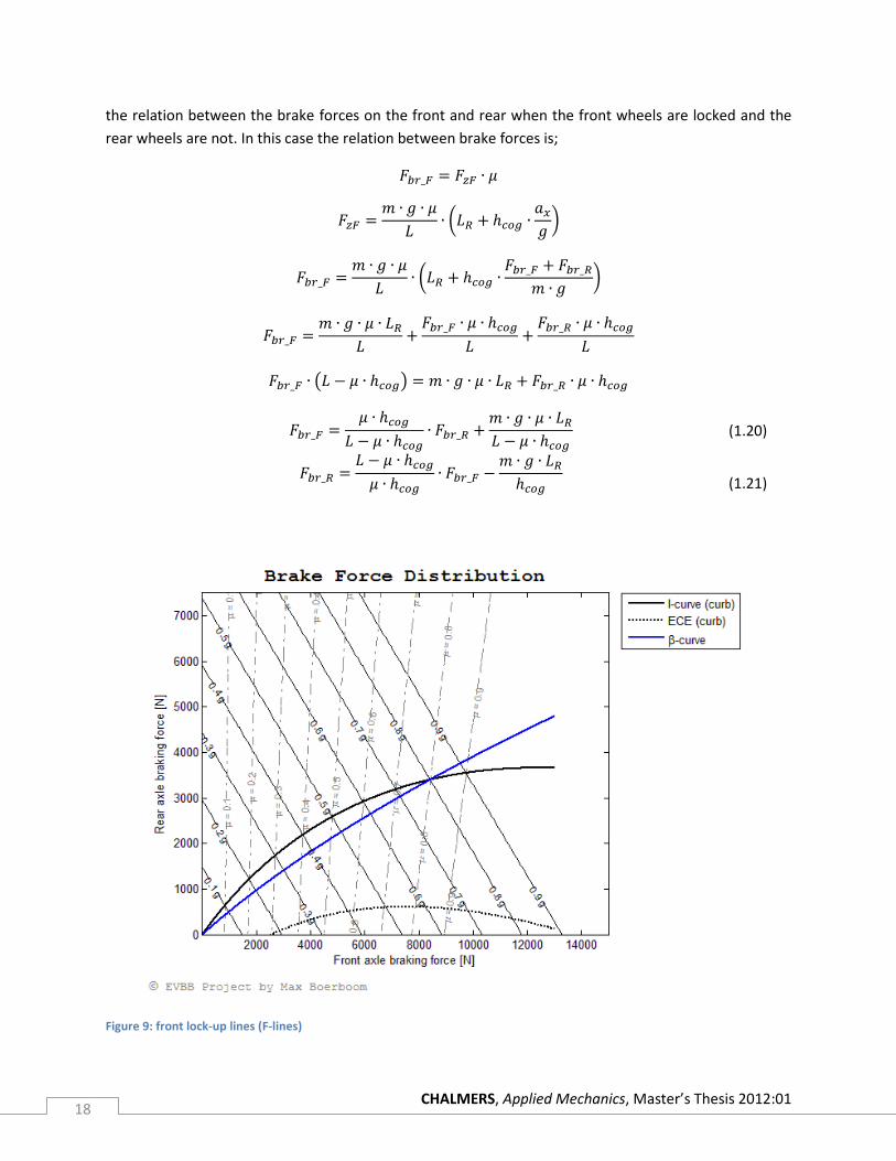
The brake forces that can be applied are limited by the tyre-ground adhesion. Along the ideal brake
force distribution (I-curve) both the front and rear wheels will lock simultaneously. Everywhere else only
one of the axles will saturate first. For the analyses of handling the relation of brake forces when one
axle locks can be drawn. These lines are often referred to as F-lines and R-lines. F-lines are representing
CHALMERS, Applied Mechanics, Master’s Thesis 2012:01 18
the relation between the brake forces on the front and rear when the front wheels are locked and the
rear wheels are not. In this case the relation between brake forces is;
(1.20)
(1.21)
Figure 9: front lock-up lines (F-lines)

CHALMERS, Applied Mechanics, Master’s Thesis 2012:01 19
In similar fashion the case where rear wheels are locked and front wheels are not results in (figure 10);
(1.22)
(1.23)
Figure 10: rear lock-up lines (R-lines)
CHALMERS, Applied Mechanics, Master’s Thesis 2012:01 20
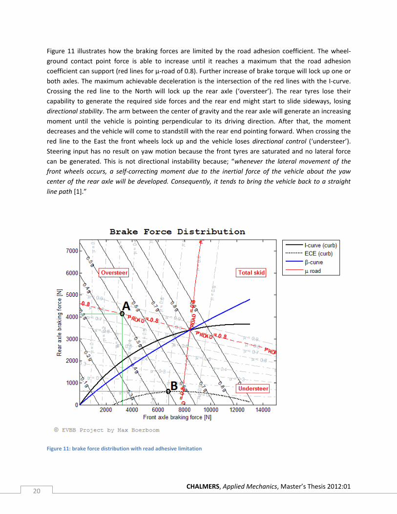
Figure 11 illustrates how the braking forces are limited by the road adhesion coefficient. The wheel-
ground contact point force is able to increase until it reaches a maximum that the road adhesion
coefficient can support (red lines for µ-road of 0.8). Further increase of brake torque will lock up one or
both axles. The maximum achievable deceleration is the intersection of the red lines with the I-curve.
Crossing the red line to the North will lock up the rear axle (‘oversteer’). The rear tyres lose their
capability to generate the required side forces and the rear end might start to slide sideways, losing
directional stability. The arm between the center of gravity and the rear axle will generate an increasing
moment until the vehicle is pointing perpendicular to its driving direction. After that, the moment
decreases and the vehicle will come to standstill with the rear end pointing forward. When crossing the
red line to the East the front wheels lock up and the vehicle loses directional control (‘understeer’).
Steering input has no result on yaw motion because the front tyres are saturated and no lateral force
can be generated. This is not directional instability because; “whenever the lateral movement of the
front wheels occurs, a self-correcting moment due to the inertial force of the vehicle about the yaw
center of the rear axle will be developed. Consequently, it tends to bring the vehicle back to a straight
line path [1].”
Figure 11: brake force distribution with read adhesive limitation
CHALMERS, Applied Mechanics, Master’s Thesis 2012:01 21
When the road adhesion equals 0.8 and the requested deceleration is 0.5 [g], the brake force
distribution could theoretically be varied between A and B, without causing direction control or
instability issues (figure 11). However, this graphical representation of the brake force distribution is for
pure longitudinal case. When braking with a force distribution A, during mild cornering, the longitudinal
brake force that can be generated is less, because lateral tyre forces are present. The brake force
distribution at B is bounded by the ECE Regulation. As will be later pointed out, this example is already
considered heavy braking, because the majority of moderate braking events are below 0.3 [g]
deceleration.
Conventional vehicles and most hybrid vehicles, available on current market, use a linear brake torque
distribution. This limits the amount of regenerative braking energy, that can be recuperated on one axle.
The response time of traditional hydraulic brakes is too slow to follow the I-curve, significantly reducing
the variability of the hybrid braking system. With the introduction of brake-by-wire systems (paragraph
1.2.4) it becomes possible to vary the distribution according the I-curve [9]. To achieve the objective of
maximizing the energy recovery, while maintaining stability and maneuverability, two optimization
problems arise:
1. The distribution of front-to-rear axle braking force, affecting the brake effectiveness and braking
stability of the vehicle.
2. The distribution between electric and mechanical braking force, which determines the ratio of
braking energy recovery [P17]. The optimal braking force distribution strategy selects a
proportioning ratio, which will satisfy the requirements of braking performance, while
maximizing the percentage of braking performed on the axle, which does regenerative braking
[P4].
CHALMERS, Applied Mechanics, Master’s Thesis 2012:01 22
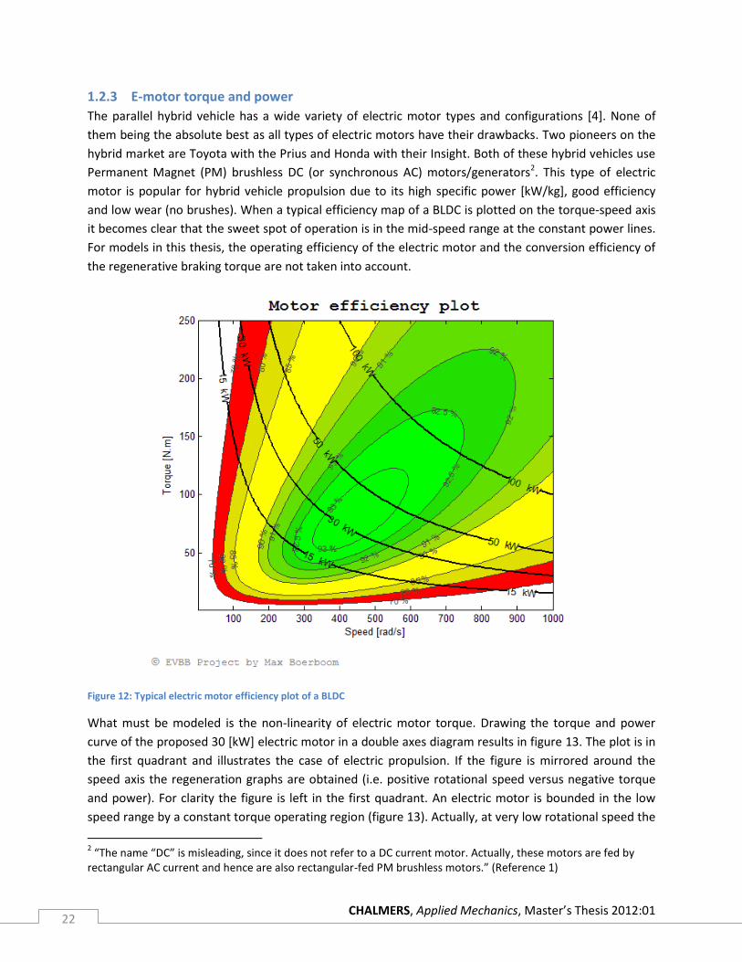
1.2.3 E-motor torque and power
The parallel hybrid vehicle has a wide variety of electric motor types and configurations [4]. None of
them being the absolute best as all types of electric motors have their drawbacks. Two pioneers on the
hybrid market are Toyota with the Prius and Honda with their Insight. Both of these hybrid vehicles use
Permanent Magnet (PM) brushless DC (or synchronous AC) motors/generators2. This type of electric
motor is popular for hybrid vehicle propulsion due to its high specific power [kW/kg], good efficiency
and low wear (no brushes). When a typical efficiency map of a BLDC is plotted on the torque-speed axis
it becomes clear that the sweet spot of operation is in the mid-speed range at the constant power lines.
For models in this thesis, the operating efficiency of the electric motor and the conversion efficiency of
the regenerative braking torque are not taken into account.
Figure 12: Typical electric motor efficiency plot of a BLDC
What must be modeled is the non-linearity of electric motor torque. Drawing the torque and power
curve of the proposed 30 [kW] electric motor in a double axes diagram results in figure 13. The plot is in
the first quadrant and illustrates the case of electric propulsion. If the figure is mirrored around the
speed axis the regeneration graphs are obtained (i.e. positive rotational speed versus negative torque
and power). For clarity the figure is left in the first quadrant. An electric motor is bounded in the low
speed range by a constant torque operating region (figure 13). Actually, at very low rotational speed the
2 “The name “DC” is misleading, since it does not refer to a DC current motor. Actually, these motors are fed by
rectangular AC current and hence are also rectangular-fed PM brushless motors.” (Reference 1)
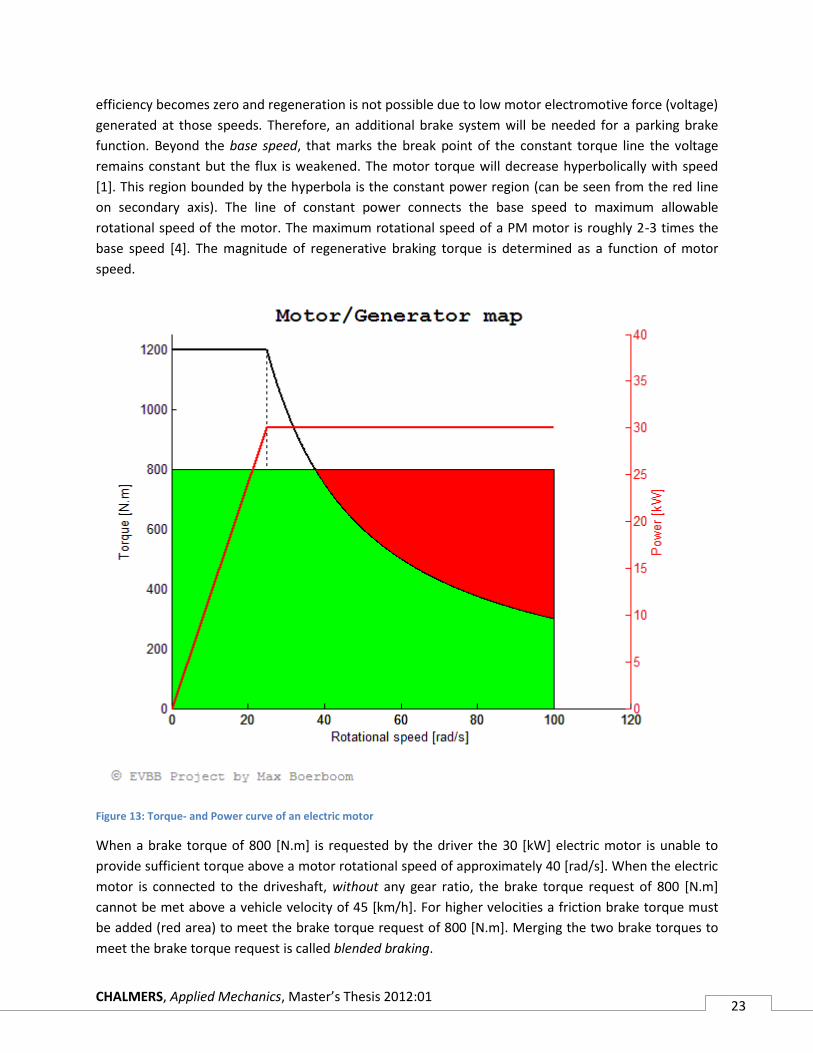
CHALMERS, Applied Mechanics, Master’s Thesis 2012:01 23
efficiency becomes zero and regeneration is not possible due to low motor electromotive force (voltage)
generated at those speeds. Therefore, an additional brake system will be needed for a parking brake
function. Beyond the base speed, that marks the break point of the constant torque line the voltage
remains constant but the flux is weakened. The motor torque will decrease hyperbolically with speed
[1]. This region bounded by the hyperbola is the constant power region (can be seen from the red line
on secondary axis). The line of constant power connects the base speed to maximum allowable
rotational speed of the motor. The maximum rotational speed of a PM motor is roughly 2-3 times the
base speed [4]. The magnitude of regenerative braking torque is determined as a function of motor
speed.
Figure 13: Torque- and Power curve of an electric motor
When a brake torque of 800 [N.m] is requested by the driver the 30 [kW] electric motor is unable to
provide sufficient torque above a motor rotational speed of approximately 40 [rad/s]. When the electric
motor is connected to the driveshaft, without any gear ratio, the brake torque request of 800 [N.m]
cannot be met above a vehicle velocity of 45 [km/h]. For higher velocities a friction brake torque must
be added (red area) to meet the brake torque request of 800 [N.m]. Merging the two brake torques to
meet the brake torque request is called blended braking.
CHALMERS, Applied Mechanics, Master’s Thesis 2012:01 24
1.2.4 Brake-by-wire
Brake actuation decoupled from the brake pedal is named brake-by-wire. Or in other words, a brake-by-
wire system is not mechanically attached to the friction brakes. The two prominent examples of brake-
by-wire systems are the Electro Hydraulic Brake (EHB) and the Electro Mechanical Brake (EMB). The EHB
is already mass produced and available on current market (e.g. Toyota Prius). Using a brake-by-wire
system is inevitable when realizing a blended brake control because the brake torques that must be
added by the friction brakes are highly variable and dependent on vehicle velocity and electric motor
state (figure 13) rather than pedal travel. An important objective when using RBS or brake-by-wire in the
vehicle is to simulate a natural pedal feel. The human perception of vehicle deceleration when
depressing the brake pedal must remain the same. In a standard brake system, the proportionality
between pedal force and pedal stroke is nonlinear; the amount of change of stroke decreases as the
pedal force increases. This feel of the brake pedal needs to be simulated for disconnected brake pedals
by means of a pedal simulator.
Electro Hydraulic Braking
Although there is no mechanical connection between the brake pedal and the caliper the EHB braking
forces at the wheels are still applied hydraulically. The EHB is the first step to the full brake-by-wire
system, which is often named as the electric or electromechanical brake.
The controller of and EHB is called a Hydraulic Electric Control Unit (HECU) and includes all modern
vehicle brake intervention and wheel slip controls (e.g. ABS, EBD, TCS, ESC, BA). To minimize the chance
of electrical faults component redundancy is used in the HECU [P7]. The hardware consists of a pedal
simulator, Hydraulic Control Unit (HCU), accumulator and modified brake calipers. Sensors that are
necessary for EHB control are wheel speeds, steer wheel angle, yaw rate, longitudinal and lateral
accelerometer, accumulator pressure sensor and pedal stroke sensor. The majority of these sensors are
already present in vehicles that have active safety systems as ABS and ESC (chapter 1.3). The pedal
stroke sensor senses the drivers’ brake intention and translates it in the HECU to the appropriate friction
brake pressure. In case EHB is combined with RBS the brake pressure control target is the subtraction of
the regenerative torque from the brake torque request generated in response to the drivers operation
of the brake pedal. The Hydraulic Control Unit (HCU) has a high pressure supply coming from a pump
and individual connections to all EHB regulated brake calipers. The main challenges of control for EHB
are; emergency braking and modulation of brake pressure. Unlike conventional brake systems that
amplify the brake force applied on the brake pedal an EHB system is dependent on a pump and
accumulator to supply the brake pressure. EHBs use a gas pressurized accumulator that stores brake
fluid under pressures ranging from 16-20 [MPa]. A separated hydraulic circuit between the wheel brakes
and the accumulator can isolate the accumulator and avoid that gas from the accumulator gets to the
calipers.
CHALMERS, Applied Mechanics, Master’s Thesis 2012:01 25
The Electric Hydraulic Brake (EHB) system has the following advantages compared to conventional brake
systems.
The relation (controlled by the HECU) between brake caliper pressure and brake pedal travel is
always the same. The brake controller is able to compensate for variation due to increased fluid
temperature and brake pad wear [P13].
The decoupled brake pedal is feedback-free. The mechanical separation between the pedal and
the brake actuator filters out disturbances that otherwise could be felt in the brake pedal.
Vibrations created during ABS modulation make some drivers assume brake malfunctions. They
will (partially) release the pedal which results in poor braking and long stopping distance.
The rate of pressure increase in panic braking situations is much higher than those obtained by a
conventional brake system because the accumulator can be set to a high pressure (16-20 MPa)
resulting in a fast response time, especially at the beginning of braking.
The dynamic response of the EHB can be optimized using so called “pre-fill” function. This pre-
pressurizes the brake system, minimizing the play and thereby improving the brake response.
This is an important advantage if the brake system is merged with a RBS because the response
time of the electric motor is generally faster than the hydraulics.
Flexibility of unequal brake force distribution, allowing integration of stability features as ESC.
Unlike conventional ESC systems (chapter 1.3.2), EHB can take advantage of the high hydraulic
pressure in the accumulator that can be rapidly transferred to individual wheels.
Packaging advantage. Mechanical components as the vacuum booster and the vacuum pump
can be removed. A vacuum pump is needed in diesel propelled vehicles because they have no
throttle valve that creates vacuum in the inlet manifold.
No dependence of the braking torques upon the engine vacuum. This makes EHB very suitable
for start-stop systems.
EHB hardware is typically implemented with series RBS. Although EHB has a faster response time than a
conventional braking system, it cannot yet quite match the response time of a RBS. This might cause a
gap in brake torque and consequently vehicle deceleration, which is noticeable to the driver. Toyota had
such problems with their 4th generation of the Prius, losing a lot of money on the recall they had to
make. An important advantage of EHB compared to other brake-by-wire systems is the fail-safe mode.
The EHB can be equipped with a redundant switchable hydraulic channel. In case of EHB system
malfunction the switch can be activated, mechanically connecting the brake pedal to the wheel brakes
(i.e. calipers). The pedal force versus vehicle deceleration will however be affected because the vacuum
booster is eliminated, but the driver will be able to bring the vehicle to a standstill without being
dependent on electronics.
CHALMERS, Applied Mechanics, Master’s Thesis 2012:01 26
Electro Mechanical Braking
The EMB is often considered a true brake-by-wire system and is also called a dry brake system, as it uses
no hydraulic components. The EMB actuation unit is entirely mounted in the unsprung mass, which
means it must be very shock resistant. Although the EMB increases the unsprung mass of the vehicle,
the complexity of hardware and overall weight of the braking system is reduced compared to others.
The Electro Mechanical Brake (EMB) system has following advantages compared to conventional and
hydraulic actuated brake systems:
No hydraulics at all, improves packaging and allows the brake pedal to be placed anywhere.
Just like the EHB the pulsations and disturbances felt in the brake pedal of a conventional brake
system due to ABS activation or uneven disc wear can be eliminated.
Adjustable brake pedal characteristics.
Similar to EHB, wheel individual brake interventions can be easily applied with a much higher
rate than conventional brake systems.
Ease of maintenance.
Even smaller response time due to eliminated hydraulic lag.
Parking brake is easier to integrate [3].
Low noise production even in the ABS mode.
However there are some drawbacks, which proved to be very hard to overcome, preventing the mass
production of EMB systems up to now.
All energy required to generate the braking force must be supplied by the vehicles electrical
system. A 42 Volt electrical system will be required to meet the power demand of the EMB.
Fail-safe mode. When the system fails there is no mechanical connection or hydraulic ‘fallback’
that can replace the brake function. This is the main legal requirement issue, avoiding large scale
production of the system.
Component cost and complexity of the system is higher than EHB.
EMB requires high speed communication (FlexRay), to provide the required system fault
tolerance.
Response time to high clamping forces (50 kN) is yet insufficient [3].
Increased wheel mass might generate vibration issues.
Small allowance of play on components, that are subjected to heavy vibrations and ambient
conditions.
The issue of too low circuit voltage in the automotive electronics arises in more fields of automotive
engineering, as the amount of electrical component keeps increasing. An example in the field of
combustion optimization is the camless valve train control by means of coils, studied by BMW and
Valeo. The discussion has been going on for quite a while to increase the board voltage to 42 Volt,
enabling the use of heavier consumers. However, up till now, the investment to entirely redefine the
board net is found too expensive and therefore not feasible. With the introduction of hybrid vehicles the
solution might be relatively easy. Hybrid drive trains need a high power circuit (power electronics), as
CHALMERS, Applied Mechanics, Master’s Thesis 2012:01 27
they operate with current and voltages far beyond that in normal automotive electronics. A separate
‘secondary’ 42 Volt board net could be made to connect the EMB, without re-designing every single
sensor. Another solution is to apply the EMB only on the axle, that is braked by the RBS. This will reduce
the power consumption of the system and make a blended brake control possible. However, when this
approach is taken, three different types of brake systems need to be merged (i.e. hydraulic, EMB and
RBS) increasing the complexity of control even more.
CHALMERS, Applied Mechanics, Master’s Thesis 2012:01 28
1.2.5 Brake energy recovery potential
The measure to which brake energy can be recovered is dependent on the motor characteristics, drive
train layout, energy storage capacity and drive train efficiencies. During a brake event the State of
Charge (SOC) will rarely be the limiting factor for energy recuperation, unless the vehicle is braking for a
long time during descent. The main restrictions are the power characteristic of the electric motor and
the charging characteristic of the battery [P6]. For small electric motors the brake torque is limited
(figure 13). However, limitation also depends on motor rotational speed, which is proportional to vehicle
velocity. This thesis looks at the idealized case, neglecting heat loses and conversion efficiency of
regenerative braking torque and focusing purely on the power and energy that can be recuperated.
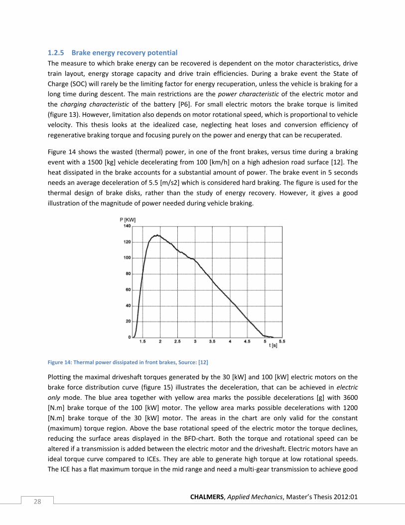
Figure 14 shows the wasted (thermal) power, in one of the front brakes, versus time during a braking
event with a 1500 [kg] vehicle decelerating from 100 [km/h] on a high adhesion road surface [12]. The
heat dissipated in the brake accounts for a substantial amount of power. The brake event in 5 seconds
needs an average deceleration of 5.5 [m/s2] which is considered hard braking. The figure is used for the
thermal design of brake disks, rather than the study of energy recovery. However, it gives a good
illustration of the magnitude of power needed during vehicle braking.
Figure 14: Thermal power dissipated in front brakes, Source: [12]
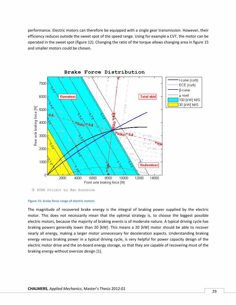
Plotting the maximal driveshaft torques generated by the 30 [kW] and 100 [kW] electric motors on the
brake force distribution curve (figure 15) illustrates the deceleration, that can be achieved in electric
only mode. The blue area together with yellow area marks the possible decelerations [g] with 3600
[N.m] brake torque of the 100 [kW] motor. The yellow area marks possible decelerations with 1200
[N.m] brake torque of the 30 [kW] motor. The areas in the chart are only valid for the constant
(maximum) torque region. Above the base rotational speed of the electric motor the torque declines,
reducing the surface areas displayed in the BFD-chart. Both the torque and rotational speed can be
altered if a transmission is added between the electric motor and the driveshaft. Electric motors have an
ideal torque curve compared to ICEs. They are able to generate high torque at low rotational speeds.
The ICE has a flat maximum torque in the mid range and need a multi-gear transmission to achieve good
CHALMERS, Applied Mechanics, Master’s Thesis 2012:01 29
performance. Electric motors can therefore be equipped with a single gear transmission. However, their
efficiency reduces outside the sweet spot of the speed range. Using for example a CVT, the motor can be
operated in the sweet spot (figure 12). Changing the ratio of the torque allows changing area in figure 15
and smaller motors could be chosen.
Figure 15: brake force range of electric motors
The magnitude of recovered brake energy is the integral of braking power supplied by the electric
motor. This does not necessarily mean that the optimal strategy is, to choose the biggest possible
electric motors, because the majority of braking events is of moderate nature. A typical driving cycle has
braking powers generally lower than 20 [kW]. This means a 20 [kW] motor should be able to recover
nearly all energy, making a larger motor unnecessary for deceleration aspects. Understanding braking
energy versus braking power in a typical driving cycle, is very helpful for power capacity design of the
electric motor drive and the on-board energy storage, so that they are capable of recovering most of the
braking energy without oversize design [1].
CHALMERS, Applied Mechanics, Master’s Thesis 2012:01 30
1.3 Active safety systems
Merging two braking systems requires a clear distinction in the hierarchy, ensuring safe operation in
emergency situations. This paragraph explains the background and working principle of the most widely
adopted active safety systems. The ABS and ESC are applied to all newly developed automobiles today.
The safety functionality of these systems needs to be maintained or improved, when regenerative
braking is introduced.
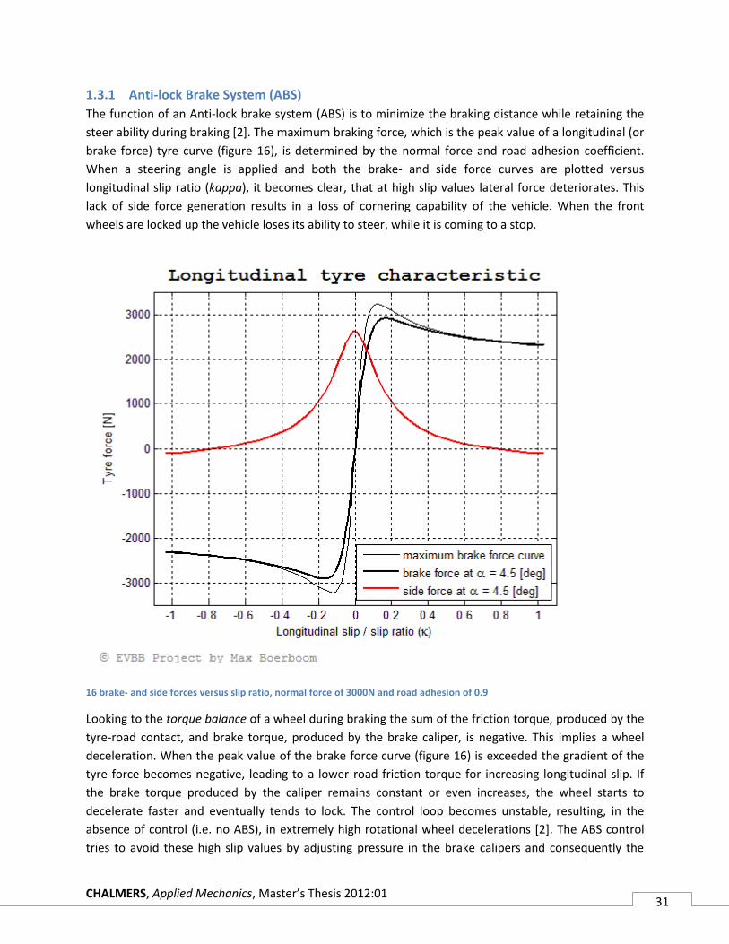
CHALMERS, Applied Mechanics, Master’s Thesis 2012:01 31
1.3.1 Anti-lock Brake System (ABS)
The function of an Anti-lock brake system (ABS) is to minimize the braking distance while retaining the
steer ability during braking [2]. The maximum braking force, which is the peak value of a longitudinal (or
brake force) tyre curve (figure 16), is determined by the normal force and road adhesion coefficient.
When a steering angle is applied and both the brake- and side force curves are plotted versus
longitudinal slip ratio (kappa), it becomes clear, that at high slip values lateral force deteriorates. This
lack of side force generation results in a loss of cornering capability of the vehicle. When the front
wheels are locked up the vehicle loses its ability to steer, while it is coming to a stop.
16 brake- and side forces versus slip ratio, normal force of 3000N and road adhesion of 0.9
Looking to the torque balance of a wheel during braking the sum of the friction torque, produced by the
tyre-road contact, and brake torque, produced by the brake caliper, is negative. This implies a wheel
deceleration. When the peak value of the brake force curve (figure 16) is exceeded the gradient of the
tyre force becomes negative, leading to a lower road friction torque for increasing longitudinal slip. If
the brake torque produced by the caliper remains constant or even increases, the wheel starts to
decelerate faster and eventually tends to lock. The control loop becomes unstable, resulting, in the
absence of control (i.e. no ABS), in extremely high rotational wheel decelerations [2]. The ABS control
tries to avoid these high slip values by adjusting pressure in the brake calipers and consequently the
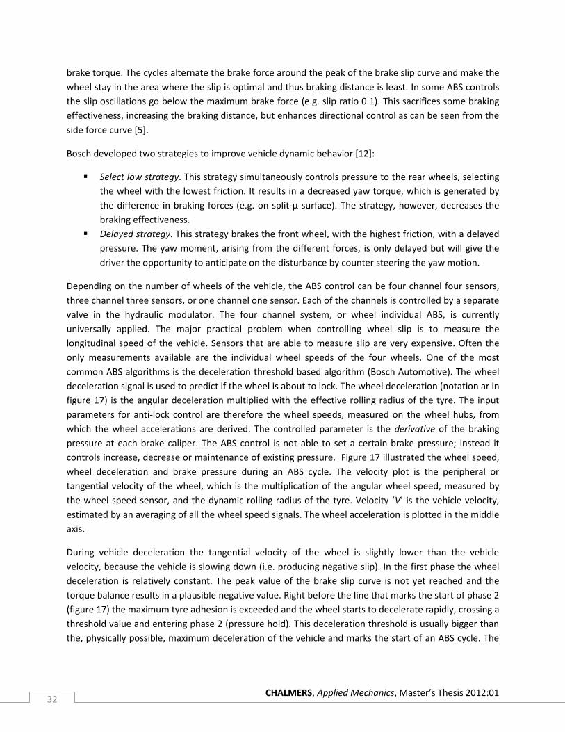
CHALMERS, Applied Mechanics, Master’s Thesis 2012:01 32
brake torque. The cycles alternate the brake force around the peak of the brake slip curve and make the
wheel stay in the area where the slip is optimal and thus braking distance is least. In some ABS controls
the slip oscillations go below the maximum brake force (e.g. slip ratio 0.1). This sacrifices some braking
effectiveness, increasing the braking distance, but enhances directional control as can be seen from the
side force curve [5].
Bosch developed two strategies to improve vehicle dynamic behavior [12]:
Select low strategy. This strategy simultaneously controls pressure to the rear wheels, selecting
the wheel with the lowest friction. It results in a decreased yaw torque, which is generated by
the difference in braking forces (e.g. on split-µ surface). The strategy, however, decreases the
braking effectiveness.
Delayed strategy. This strategy brakes the front wheel, with the highest friction, with a delayed
pressure. The yaw moment, arising from the different forces, is only delayed but will give the
driver the opportunity to anticipate on the disturbance by counter steering the yaw motion.
Depending on the number of wheels of the vehicle, the ABS control can be four channel four sensors,
three channel three sensors, or one channel one sensor. Each of the channels is controlled by a separate
valve in the hydraulic modulator. The four channel system, or wheel individual ABS, is currently
universally applied. The major practical problem when controlling wheel slip is to measure the
longitudinal speed of the vehicle. Sensors that are able to measure slip are very expensive. Often the
only measurements available are the individual wheel speeds of the four wheels. One of the most
common ABS algorithms is the deceleration threshold based algorithm (Bosch Automotive). The wheel
deceleration signal is used to predict if the wheel is about to lock. The wheel deceleration (notation ar in
figure 17) is the angular deceleration multiplied with the effective rolling radius of the tyre. The input
parameters for anti-lock control are therefore the wheel speeds, measured on the wheel hubs, from
which the wheel accelerations are derived. The controlled parameter is the derivative of the braking
pressure at each brake caliper. The ABS control is not able to set a certain brake pressure; instead it
controls increase, decrease or maintenance of existing pressure. Figure 17 illustrated the wheel speed,
wheel deceleration and brake pressure during an ABS cycle. The velocity plot is the peripheral or
tangential velocity of the wheel, which is the multiplication of the angular wheel speed, measured by
the wheel speed sensor, and the dynamic rolling radius of the tyre. Velocity ‘V’ is the vehicle velocity,
estimated by an averaging of all the wheel speed signals. The wheel acceleration is plotted in the middle
axis.
During vehicle deceleration the tangential velocity of the wheel is slightly lower than the vehicle
velocity, because the vehicle is slowing down (i.e. producing negative slip). In the first phase the wheel
deceleration is relatively constant. The peak value of the brake slip curve is not yet reached and the
torque balance results in a plausible negative value. Right before the line that marks the start of phase 2
(figure 17) the maximum tyre adhesion is exceeded and the wheel starts to decelerate rapidly, crossing a
threshold value and entering phase 2 (pressure hold). This deceleration threshold is usually bigger than
the, physically possible, maximum deceleration of the vehicle and marks the start of an ABS cycle. The
CHALMERS, Applied Mechanics, Master’s Thesis 2012:01 33
pressure hold in the first cycle is to suppress noise influences and road disturbances. ABS modulation of
the brake line pressure occurs at approximately 15 (Hz) [6].
Figure 17: ABS cycle, Source [12]
A detailed explanation of the control phases in the ABS cycle, illustrated in the figure 17, can be found in
‘The Automotive Chassis Volume 1’ by G. Genta and L. Morello [12].
The anti-lock braking control is always dominant over the Electronic Stability Control (ESC). That means,
when differential braking forces are applied by the ESC and a wheel drops below the threshold value of
wheel deceleration, the ABS control will be activated. Limitation of anti-lock braking is that it performs
badly on gravel or fresh snow surfaces. These road surfaces tend to form a wedge in front of the locked
up wheels that causes a braking effect. On deformable surfaces like gravel, the coefficient of friction
increases monotonically until it reaches a maximum at wheel lock [P15]. It must however be emphasized
that ABS activation is a rare occurrence and these system limitations are of little relevance to daily
driving. In such cases, the improved steer ability provided by the control is more important than the
shortest stopping distance. On a low adhesion surface the stopping distance will always be larger than
CHALMERS, Applied Mechanics, Master’s Thesis 2012:01 34
on high adhesion surfaces, as the maximum braking force is dependent on the friction between the road
and tyres. When curves are taken too fast, even a vehicle with ABS might slide of the road.
The transition to electrification of the braking system has some promising improvements with respect to
ABS control. Where a conventional hydraulic braking system ensures correct slip ratio by pulsation of
the brake pressure, an electronically actuated brake or generator could be controlled in a continuous
manner [P13]. This way the brake regulates the pressure (or torque), rather than rate of pressure
change. The fast control of electronics eliminates the hydraulic lag. Secondly, ABS pulsations transmitted
to the brake pedal make inexperienced drivers presume brake malfunction. As a result they tend to
reduce the pedal force, resulting in poor brake utilization. The electronic brake is disconnected from the
brake pedal and makes brake control independent of pedal feel.
A summary of factors influencing the working of the ABS system:
Road adhesion coefficient, since it influences the range within which the wheel slip ratio should
be maintained.
Rate of application of the brake torque. Initially this is dependent on the pedal pressing by the
driver. When the ABS control is activated it depends on the pressure build characteristics of the
hydraulic modulator (e.g. pressure build up, response time, etc.).
Initial velocity of the vehicle, since it determines how quickly the vehicle can come to a stop.
Brake force distribution from front to rear. The maximum brake effectiveness can be obtained
with the ideal force distribution. This is an important factor in the study of regenerative braking
because during moderate braking events the utilization of the generator should be as much as
possible. This means a reduced dissipation of kinetic energy as wasted heat.
CHALMERS, Applied Mechanics, Master’s Thesis 2012:01 35
1.3.2 Electronic Stability Control (ESC)
The function of the Electronics Stability Control (ESC) is to restore the yaw rate, requested by the driver,
as much as possible. The system has numerous commercial names as; Electronic Stability Program (ESP),
Dynamic Stability Control (DCS), Vehicle Dynamics Control (VDC), Vehicle Stability Control (VSC) or Yaw
Control. The latter being, in the opinion of the author, the most suited name because the system does
not directly control the stability of the vehicle but affects the yaw motion of the vehicle.
At limits of tyre adhesion the response of yaw moment to changes in steering angle is reduced. That
means that at large slip angles, changing the steering angle produces very little change in the yaw rate of
the vehicle [11]. The aim of the ESC is to reduce the deviation of vehicle behavior to its requested
behavior, by preventing the vehicle slip angle to become large. Simulating the control of yaw dynamics
can be accomplished by a reduced non-linear two track model. Larger simplification to a single track
model is not possible because of differential torques and adhesion losses on one side of the vehicle. The
non-linearity should be introduced, to simulate the loss of traction.
Three different types of yaw control can be distinguished:
Differential brake torque
Active steering
Differential propulsion torque (i.e. torque vectoring)
The first mentioned is by far the most applied stability control system. This system is low cost and has a
high robustness and reliability compared to the others. As mentioned in the proposal of actuator
configurations (paragraph 1.1.2) an individual four-wheel electric motor drive train can be used with ESC
torque distribution (torque vectoring) strategy. However, this drive train lay-out is out of scope of this
thesis. The differential braking control utilizes the hydraulic modulator from the ABS, to apply unequal
brake pressures between the right- and left hand side of the vehicle, initiating non-symmetrical brake
torques that produce a yaw moment. The friction brakes are therefore not only suitable to decrease the
longitudinal velocity of the vehicle, but can also be used to change the vehicle path. In case the intended
body slip angle (β) of the vehicle is not reached, the driver will react by a steering input (δ). In a critical
situation a short braking event on one of the wheels can correct the body slip angle. On dry asphalt the
maneuverability on the vehicle is lost, when the body slip angle is greater than 10 degrees, while on
slippery surfaces the maneuverability can be lost with a body slip angle as small as 4 degrees [11]. When
yaw offset exceeds a threshold the ESC controller commands one wheel to be braked. During
understeered behavior (paragraph 1.2.1) the vehicle makes a larger radius than intended by the driver,
because the front wheels reached the traction limit. Braking the inner rear wheel creates a yaw moment
that decreases the path curvature. Oversteered behavior occurs when the rear end saturates and can be
compensated by outer front wheel braking.
CHALMERS, Applied Mechanics, Master’s Thesis 2012:01 36
Sensors and components necessary for yaw control [12]:
Brake actuators (i.e. calipers)
Master pump (shared with ABS and EBD)
Wheel speed sensors (shared with ABS and EBD)
Hydraulic pressure modulator (shared with ABS and EBD)
Steering wheel angle sensor
Yaw rate sensor
Lateral acceleration sensor
Controller
The last four mentioned are the sensors and control used to identify parameters describing the lateral
dynamics. Current state and desired motion must be known to control the lateral dynamics. The sensors
(steering wheel angle, yaw rate, lateral acceleration) measure the current motion of the vehicle. The
desired or target motion of the vehicle is calculated in the controller, using a linear single track model.
This target motion is dependent on the steering angle and the vehicle velocity. Approximately 95% of
the lateral acceleration values, which occur under normal driving conditions, are less than 3.5 [m/s2].
This is within the validity range of the linear single track model [3]. The single track equations used to
calculate target motion are:
ψ (1.24)
ψ (1.25)
(1.26)
(1.27)
ψ
(1.28)
ψ
(1.29)
With; m = vehicle mass [kg], V = velocity [m/s], ψ = yaw rate [rad/s], F = force [N], Iz = moment of inertia [kg.m2],
Lf = CoG to front axle [m], Lr = CoG to rear axle [m], C = cornering stiffness [N/rad], α = tyre slip angle [rad], δ =
steering angle [rad] and suffixes x,y,F,R = longitudinal, lateral, Front, Rear respectively.
Cornering stiffness is a variable of normal load and is assumed to be a constant (at nominal normal
load). The cornering stiffness is the slope of the side slip curve at the origin. A reasonable value of
CHALMERS, Applied Mechanics, Master’s Thesis 2012:01 37
cornering stiffness for a passenger car would be around 30 000 [N/rad]. When the curve fitting
parameters from the tyre empirical data file are known, the dependency of cornering stiffness upon
normal load with zero side slip can be calculated. The formula for cornering stiffness is [13]:
The yaw rate and body slip angle can also be approximated by the steady state gains. These are the
responses of yaw rate (ψ) and body slip angle (β) for a unit change of steering angle (δ);
ψ
(1.30)
(1.31)
With stability factor (K) and B-coefficient,
(1.32)
(1.33)
With; L = wheelbase [m], g = gravitational acceleration [m/s2], η = understeer gradient [-].
The desired yaw rate cannot always be obtained, because the maximum yaw moment is dependent on
road adhesion. The target yaw rate is therefore bounded by a function of the tyre-road coefficient.
When braking on a slip-µ surface, the brake pressures supplies to the high friction side have a certain
delay. This results in a more gradual increase of yaw moment, which gives the driver time to stabilize the
vehicle by correcting the steering wheel input. The anti-lock brake control is dominant over ESC. That
means, when a differential torque is applied and the wheel tends to lock, the ABS will be activated. All
regenerative braking systems, designed by Bosch, have the function to limit regenerative brake force
application, when critical stability conditions are predicted by the ESC controller [P10].
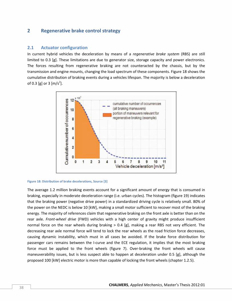
CHALMERS, Applied Mechanics, Master’s Thesis 2012:01 38
2 Regenerative brake control strategy
2.1 Actuator configuration
In current hybrid vehicles the deceleration by means of a regenerative brake system (RBS) are still
limited to 0.3 [g]. These limitations are due to generator size, storage capacity and power electronics.
The forces resulting from regenerative braking are not counteracted by the chassis, but by the
transmission and engine mounts, changing the load spectrum of these components. Figure 18 shows the
cumulative distribution of braking events during a vehicles lifespan. The majority is below a deceleration
of 0.3 [g] or 3 [m/s2].
Figure 18: Distribution of brake decelerations, Source [3]
The average 1.2 million braking events account for a significant amount of energy that is consumed in
braking, especially in moderate deceleration range (i.e. urban cycles). The histogram (figure 19) indicates
that the braking power (negative drive power) in a standardized driving cycle is relatively small. 80% of
the power on the NEDC is below 10 [kW], making a small motor sufficient to recover most of the braking
energy. The majority of references claim that regenerative braking on the front axle is better than on the
rear axle. Front-wheel drive (FWD) vehicles with a high center of gravity might produce insufficient
normal force on the rear wheels during braking > 0.4 [g], making a rear RBS not very efficient. The
decreasing rear axle normal force will tend to lock the rear wheels as the road friction force decreases,
causing dynamic instability, which must in all cases be avoided. If the brake force distribution for
passenger cars remains between the I-curve and the ECE regulation, it implies that the most braking
force must be applied to the front wheels (figure 7). Over-braking the front wheels will cause
maneuverability issues, but is less suspect able to happen at deceleration under 0.5 [g], although the
proposed 100 [kW] electric motor is more than capable of locking the front wheels (chapter 1.2.5).
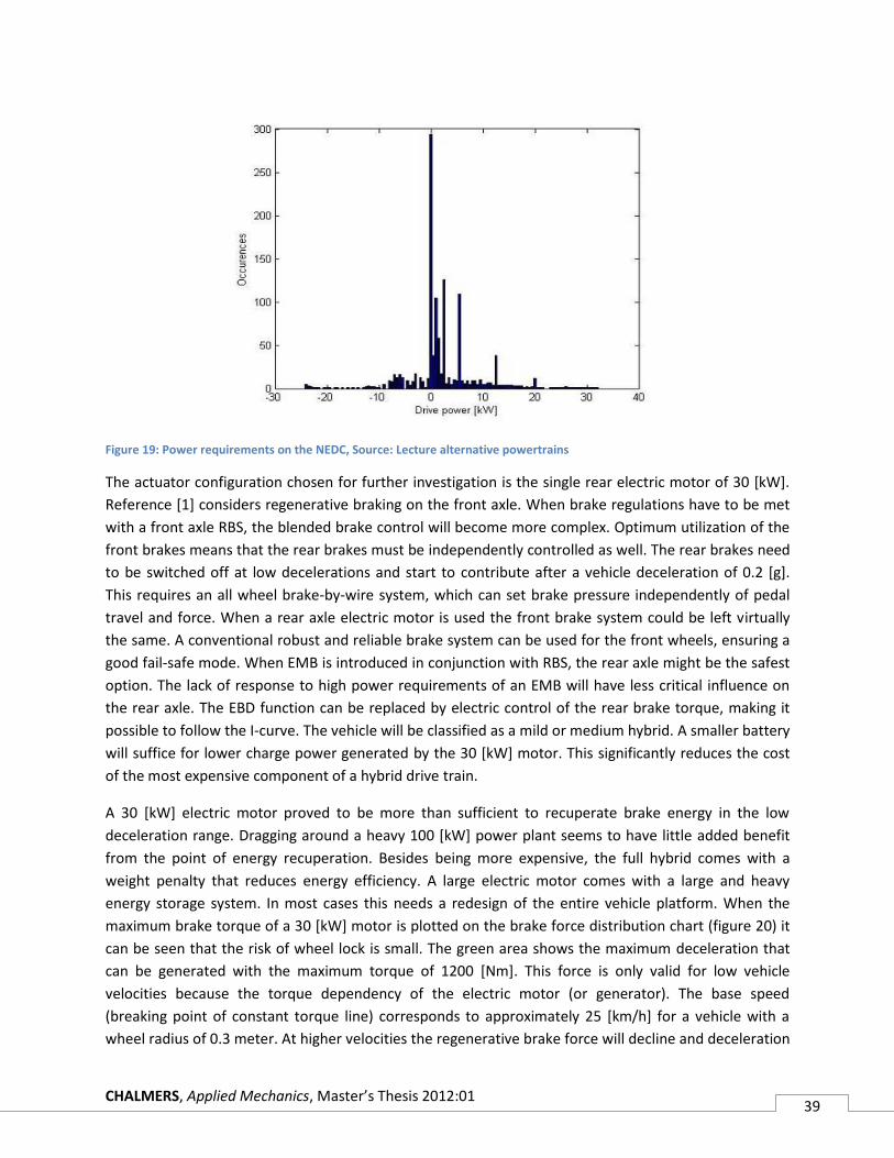
CHALMERS, Applied Mechanics, Master’s Thesis 2012:01 39
Figure 19: Power requirements on the NEDC, Source: Lecture alternative powertrains
The actuator configuration chosen for further investigation is the single rear electric motor of 30 [kW].
Reference [1] considers regenerative braking on the front axle. When brake regulations have to be met
with a front axle RBS, the blended brake control will become more complex. Optimum utilization of the
front brakes means that the rear brakes must be independently controlled as well. The rear brakes need
to be switched off at low decelerations and start to contribute after a vehicle deceleration of 0.2 [g].
This requires an all wheel brake-by-wire system, which can set brake pressure independently of pedal
travel and force. When a rear axle electric motor is used the front brake system could be left virtually
the same. A conventional robust and reliable brake system can be used for the front wheels, ensuring a
good fail-safe mode. When EMB is introduced in conjunction with RBS, the rear axle might be the safest
option. The lack of response to high power requirements of an EMB will have less critical influence on
the rear axle. The EBD function can be replaced by electric control of the rear brake torque, making it
possible to follow the I-curve. The vehicle will be classified as a mild or medium hybrid. A smaller battery
will suffice for lower charge power generated by the 30 [kW] motor. This significantly reduces the cost
of the most expensive component of a hybrid drive train.
A 30 [kW] electric motor proved to be more than sufficient to recuperate brake energy in the low
deceleration range. Dragging around a heavy 100 [kW] power plant seems to have little added benefit
from the point of energy recuperation. Besides being more expensive, the full hybrid comes with a
weight penalty that reduces energy efficiency. A large electric motor comes with a large and heavy
energy storage system. In most cases this needs a redesign of the entire vehicle platform. When the
maximum brake torque of a 30 [kW] motor is plotted on the brake force distribution chart (figure 20) it
can be seen that the risk of wheel lock is small. The green area shows the maximum deceleration that
can be generated with the maximum torque of 1200 [Nm]. This force is only valid for low vehicle
velocities because the torque dependency of the electric motor (or generator). The base speed
(breaking point of constant torque line) corresponds to approximately 25 [km/h] for a vehicle with a
wheel radius of 0.3 meter. At higher velocities the regenerative brake force will decline and deceleration

CHALMERS, Applied Mechanics, Master’s Thesis 2012:01 40
moves to a ‘safer’ area of the brake force distribution chart illustrated, by the black arrows in the chart.
The ECE regulation states that wheel lock is allowed, although not desired at vehicle velocities lower
than 20 [km/h]. When the deceleration areas on the brake force distribution chart are compared with
the cumulative brake events (figure 18) it becomes clear that a 30 [kW] generator can provide sufficient
brake force. However, it might be not recommended to only utilize the rear brakes. The force
distribution will move up along the vertical axis as regenerative brake forces are only initiated at the
rear axle. The distribution presented in the graph is for pure longitudinal deceleration. The lateral
dynamics can be included by describing the force distribution in a dynamics square [P18].
Figure 20: 30 [kW] electric motor torque on brake force distribution curve
The proposed drive train is a torque-coupling parallel hybrid drive train with separate axle architecture
(figure 21). The front axle is powered by the internal combustion engine (ICE) and the rear axle by the
electric motor. The tractive forces produced by the two power trains are added through the vehicle
chassis and the road. The absence of a mechanical (power) connection between both power trains
offers some advantages, with respect to weight, simplicity and packaging. It keeps the ICE and
(multigear-) transmission unaltered and adds an electric traction system on the other axle. It is also a
four-wheel drive, which improves the traction on slippery roads and reduces the tractive effort on a
single tyre. The energy storage system will mainly be charged by regenerative braking. Best recuperation
performance can be achieved with a blended braking system. If the RBS charge is insufficient the rear
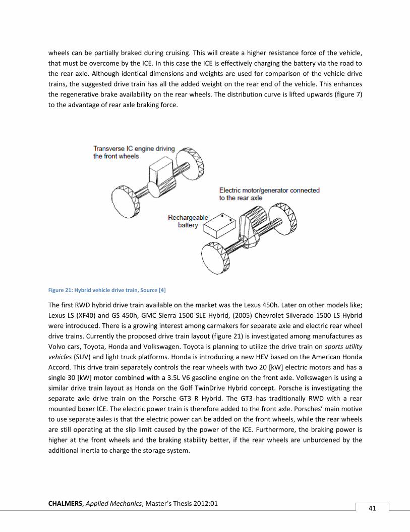
CHALMERS, Applied Mechanics, Master’s Thesis 2012:01 41
wheels can be partially braked during cruising. This will create a higher resistance force of the vehicle,
that must be overcome by the ICE. In this case the ICE is effectively charging the battery via the road to
the rear axle. Although identical dimensions and weights are used for comparison of the vehicle drive
trains, the suggested drive train has all the added weight on the rear end of the vehicle. This enhances
the regenerative brake availability on the rear wheels. The distribution curve is lifted upwards (figure 7)
to the advantage of rear axle braking force.
Figure 21: Hybrid vehicle drive train, Source [4]
The first RWD hybrid drive train available on the market was the Lexus 450h. Later on other models like;
Lexus LS (XF40) and GS 450h, GMC Sierra 1500 SLE Hybrid, (2005) Chevrolet Silverado 1500 LS Hybrid
were introduced. There is a growing interest among carmakers for separate axle and electric rear wheel
drive trains. Currently the proposed drive train layout (figure 21) is investigated among manufactures as
Volvo cars, Toyota, Honda and Volkswagen. Toyota is planning to utilize the drive train on sports utility
vehicles (SUV) and light truck platforms. Honda is introducing a new HEV based on the American Honda
Accord. This drive train separately controls the rear wheels with two 20 [kW] electric motors and has a
single 30 [kW] motor combined with a 3.5L V6 gasoline engine on the front axle. Volkswagen is using a
similar drive train layout as Honda on the Golf TwinDrive Hybrid concept. Porsche is investigating the
separate axle drive train on the Porsche GT3 R Hybrid. The GT3 has traditionally RWD with a rear
mounted boxer ICE. The electric power train is therefore added to the front axle. Porsches’ main motive
to use separate axles is that the electric power can be added on the front wheels, while the rear wheels
are still operating at the slip limit caused by the power of the ICE. Furthermore, the braking power is
higher at the front wheels and the braking stability better, if the rear wheels are unburdened by the
additional inertia to charge the storage system.

CHALMERS, Applied Mechanics, Master’s Thesis 2012:01 42
2.2 Proposed control strategies
In this paragraph three control strategies from a pure theoretical perspective are be proposed. The most
profitable solution of regenerative braking is to fully utilize the RBS. This means that at low
decelerations (< 0.25 [g]) all brake torque will be applied by the 30 [kW] motor on the rear axle (figure
23). Little margin is left to the area that marks oversteered behavior, although it shouldn’t be any
problem for high road adhesion and electric motor torques below maximum. To avoid any unwanted
stability issues, the second proposed control strategy is to follow the I-curve. This makes RBS suited to
contribute in much higher decelerations and minimizes the probability of oversteer. The accuracy and
quick response of the electric motor make it possible to bend the distribution to follow the hyperbolic
curve. The third strategy takes into account that the brake force distribution as illustrated in figure 23 is
for pure longitudinal deceleration. When braking during cornering, the margin to instability is smaller,
because some of the friction capacity of the tyres goes to the tyre side forces. Excessive braking on the
rear axle could lead to dynamic oversteer (chapter 1.2.1). The steering angle [δ] determines whether a
vehicle is cornering and is measured by the steer wheel sensor of the ESC. The strategy proposes to use
the brake distribution of strategy 1 for straight-line braking and decrease the effort of the RBS when the
steering angle is non-zero (figure 22).
Figure 22: Decrease of RBS torque with increased steering wheel angle
The power of the generator is generally too low to entirely lock both wheels on the same axle, because
the regenerative brake torque must overcome the friction torque created by both tyres. The decreased
efficiency around zero rotational speed, due to field weakening of permanent magnet (PM) motors
around the locking region makes it hard for the generator to lock the wheels. Therefore all control
strategies are proposed to switch-off the regenerative brake, when the wheel tends to lock. The loss of
brake torque will be substituted by the hydraulic system.
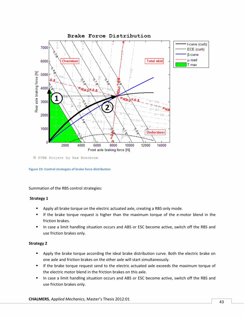
CHALMERS, Applied Mechanics, Master’s Thesis 2012:01 43
Figure 23: Control strategies of brake force distribution
Summation of the RBS control strategies:
Strategy 1
Apply all brake torque on the electric actuated axle, creating a RBS only mode.
If the brake torque request is higher than the maximum torque of the e-motor blend in the
friction brakes.
In case a limit handling situation occurs and ABS or ESC become active, switch off the RBS and
use friction brakes only.
Strategy 2
Apply the brake torque according the ideal brake distribution curve. Both the electric brake on
one axle and friction brakes on the other axle will start simultaneously.
If the brake torque request send to the electric actuated axle exceeds the maximum torque of
the electric motor blend in the friction brakes on this axle.
In case a limit handling situation occurs and ABS or ESC become active, switch off the RBS and
use friction brakes only.
CHALMERS, Applied Mechanics, Master’s Thesis 2012:01 44
Strategy 3
Apply all brake torque on the electric actuated axle with the condition that the steering angle is
small.
If the brake torque request is higher than the maximum torque of the e-motor blend in the
friction brakes.
When the steering angle is large reduce the contribution of the RBS and use friction brakes
instead.
In case a limit handling situation occurs and ABS or ESC become active, switch off the RBS and
use friction brakes only.
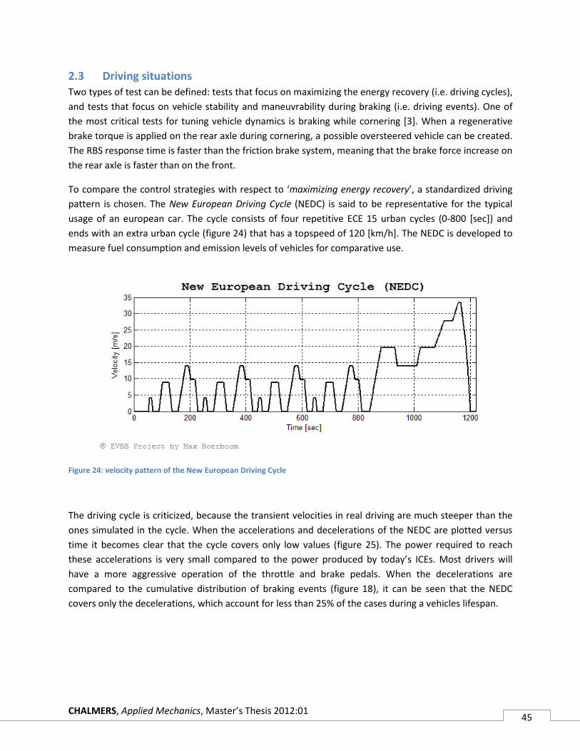
CHALMERS, Applied Mechanics, Master’s Thesis 2012:01 45
2.3 Driving situations
Two types of test can be defined: tests that focus on maximizing the energy recovery (i.e. driving cycles),
and tests that focus on vehicle stability and maneuvrability during braking (i.e. driving events). One of
the most critical tests for tuning vehicle dynamics is braking while cornering [3]. When a regenerative
brake torque is applied on the rear axle during cornering, a possible oversteered vehicle can be created.
The RBS response time is faster than the friction brake system, meaning that the brake force increase on
the rear axle is faster than on the front.
To compare the control strategies with respect to ‘maximizing energy recovery’, a standardized driving
pattern is chosen. The New European Driving Cycle (NEDC) is said to be representative for the typical
usage of an european car. The cycle consists of four repetitive ECE 15 urban cycles (0-800 [sec]) and
ends with an extra urban cycle (figure 24) that has a topspeed of 120 [km/h]. The NEDC is developed to
measure fuel consumption and emission levels of vehicles for comparative use.
Figure 24: velocity pattern of the New European Driving Cycle
The driving cycle is criticized, because the transient velocities in real driving are much steeper than the
ones simulated in the cycle. When the accelerations and decelerations of the NEDC are plotted versus
time it becomes clear that the cycle covers only low values (figure 25). The power required to reach
these accelerations is very small compared to the power produced by today’s ICEs. Most drivers will
have a more aggressive operation of the throttle and brake pedals. When the decelerations are
compared to the cumulative distribution of braking events (figure 18), it can be seen that the NEDC
covers only the decelerations, which account for less than 25% of the cases during a vehicles lifespan.
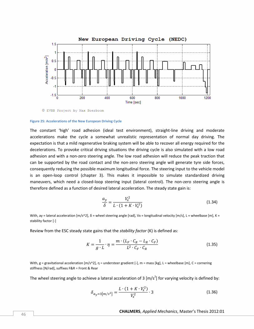
CHALMERS, Applied Mechanics, Master’s Thesis 2012:01 46
Figure 25: Accelerations of the New European Driving Cycle
The constant ‘high’ road adhesion (ideal test environment), straight-line driving and moderate
accelerations make the cycle a somewhat unrealistic representation of normal day driving. The
expectation is that a mild regenerative braking system will be able to recover all energy required for the
decelerations. To provoke critical driving situations the driving cycle is also simulated with a low road
adhesion and with a non-zero steering angle. The low road adhesion will reduce the peak traction that
can be supported by the road contact and the non-zero steering angle will generate tyre side forces,
consequently reducing the possible maximum longitudinal force. The steering input to the vehicle model
is an open-loop control (chapter 3). This makes it impossible to simulate standardized driving
maneuvers, which need a closed-loop steering input (lateral control). The non-zero steering angle is
therefore defined as a function of desired lateral acceleration. The steady state gain is:
(1.34)
With, ay = lateral acceleration [m/s^2], δ = wheel steering angle [rad], Vx = longitudinal velocity [m/s], L = wheelbase [m], K =
stability factor [-]
Review from the ESC steady state gains that the stability factor (K) is defined as:
(1.35)
With, g = gravitational acceleration [m/s^2], η = understeer gradient [-], m = mass [kg], L = wheelbase [m], C = cornering
stiffness [N/rad], suffixes F&R = Front & Rear
The wheel steering angle to achieve a lateral acceleration of 3 [m/s2] for varying velocity is defined by:
(1.36)
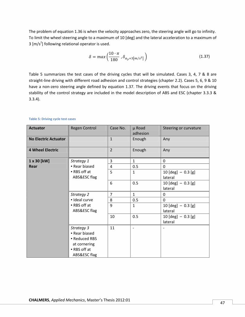
CHALMERS, Applied Mechanics, Master’s Thesis 2012:01 47
The problem of equation 1.36 is when the velocity approaches zero, the steering angle will go to infinity.
To limit the wheel steering angle to a maximum of 10 [deg] and the lateral acceleration to a maximum of
3 [m/s2] following relational operator is used.
(1.37)
Table 5 summarizes the test cases of the driving cycles that will be simulated. Cases 3, 4, 7 & 8 are
straight-line driving with different road adhesion and control strategies (chapter 2.2). Cases 5, 6, 9 & 10
have a non-zero steering angle defined by equation 1.37. The driving events that focus on the driving
stability of the control strategy are included in the model description of ABS and ESC (chapter 3.3.3 &
3.3.4).
Table 5: Driving cycle test cases
Actuator Regen Control Case No. µ Road adhesion
Steering or curvature
No Electric Actuator 1 Enough Any
4 Wheel Electric 2 Enough Any
1 x 30 [kW] Rear
Strategy 1 ▪ Rear biased ▪ RBS off at ABS&ESC flag
3 1 0
4 0.5 0
5 1 10 [deg] – 0.3 [g] lateral
6 0.5 10 [deg] – 0.3 [g] lateral
Strategy 2 ▪ Ideal curve ▪ RBS off at ABS&ESC flag
7 1 0
8 0.5 0
9 1 10 [deg] – 0.3 [g] lateral
10 0.5 10 [deg] – 0.3 [g] lateral
Strategy 3 ▪ Rear biased ▪ Reduced RBS at cornering ▪ RBS off at ABS&ESC flag
11 - -
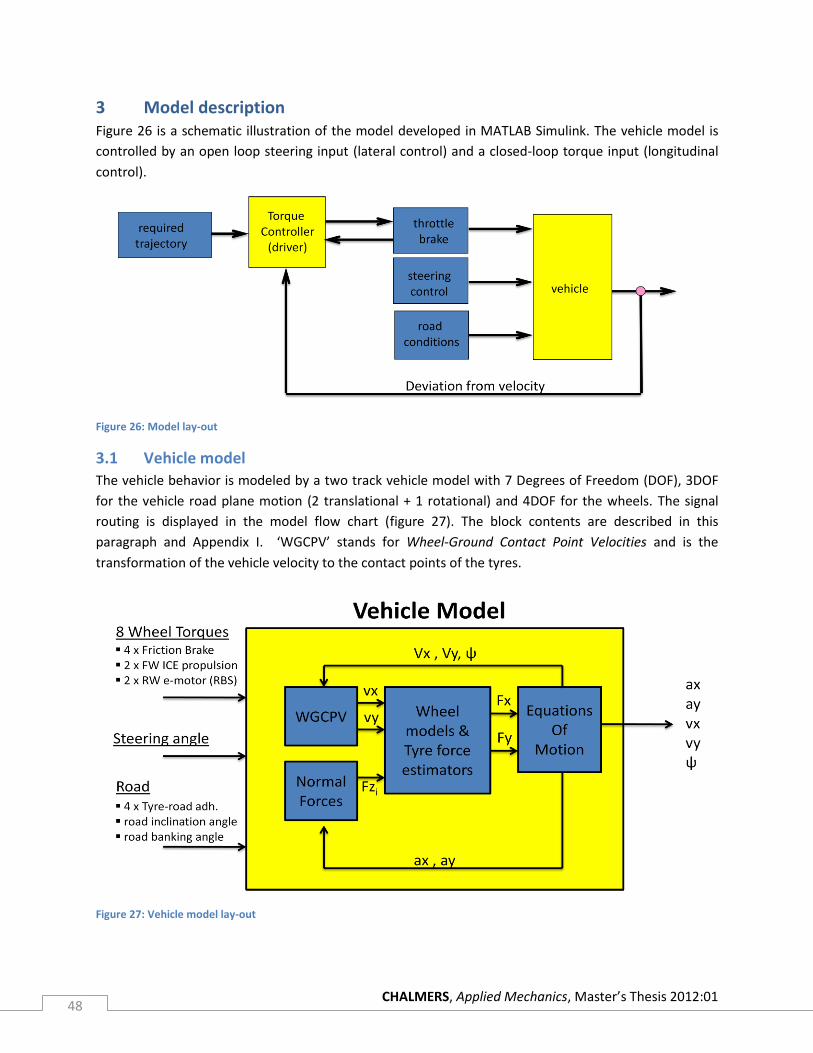
CHALMERS, Applied Mechanics, Master’s Thesis 2012:01 48
3 Model description Figure 26 is a schematic illustration of the model developed in MATLAB Simulink. The vehicle model is
controlled by an open loop steering input (lateral control) and a closed-loop torque input (longitudinal
control).
Figure 26: Model lay-out
3.1 Vehicle model
The vehicle behavior is modeled by a two track vehicle model with 7 Degrees of Freedom (DOF), 3DOF
for the vehicle road plane motion (2 translational + 1 rotational) and 4DOF for the wheels. The signal
routing is displayed in the model flow chart (figure 27). The block contents are described in this
paragraph and Appendix I. ‘WGCPV’ stands for Wheel-Ground Contact Point Velocities and is the
transformation of the vehicle velocity to the contact points of the tyres.
Figure 27: Vehicle model lay-out
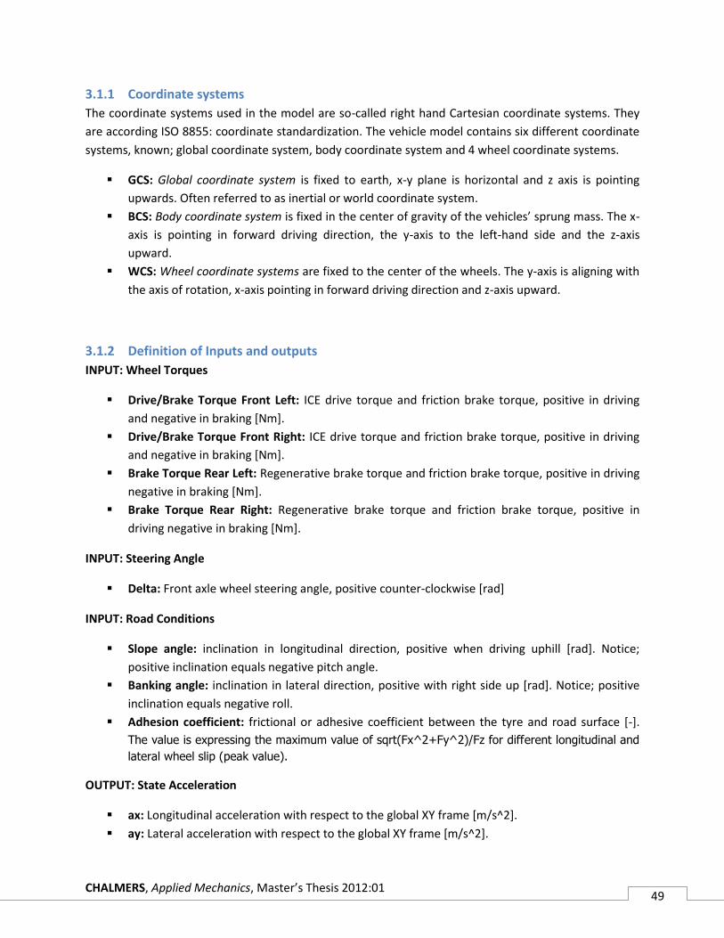
CHALMERS, Applied Mechanics, Master’s Thesis 2012:01 49
3.1.1 Coordinate systems
The coordinate systems used in the model are so-called right hand Cartesian coordinate systems. They
are according ISO 8855: coordinate standardization. The vehicle model contains six different coordinate
systems, known; global coordinate system, body coordinate system and 4 wheel coordinate systems.
GCS: Global coordinate system is fixed to earth, x-y plane is horizontal and z axis is pointing
upwards. Often referred to as inertial or world coordinate system.
BCS: Body coordinate system is fixed in the center of gravity of the vehicles’ sprung mass. The x-
axis is pointing in forward driving direction, the y-axis to the left-hand side and the z-axis
upward.
WCS: Wheel coordinate systems are fixed to the center of the wheels. The y-axis is aligning with
the axis of rotation, x-axis pointing in forward driving direction and z-axis upward.
3.1.2 Definition of Inputs and outputs
INPUT: Wheel Torques
Drive/Brake Torque Front Left: ICE drive torque and friction brake torque, positive in driving
and negative in braking [Nm].
Drive/Brake Torque Front Right: ICE drive torque and friction brake torque, positive in driving
and negative in braking [Nm].
Brake Torque Rear Left: Regenerative brake torque and friction brake torque, positive in driving
negative in braking [Nm].
Brake Torque Rear Right: Regenerative brake torque and friction brake torque, positive in
driving negative in braking [Nm].
INPUT: Steering Angle
Delta: Front axle wheel steering angle, positive counter-clockwise [rad]
INPUT: Road Conditions
Slope angle: inclination in longitudinal direction, positive when driving uphill [rad]. Notice;
positive inclination equals negative pitch angle.
Banking angle: inclination in lateral direction, positive with right side up [rad]. Notice; positive
inclination equals negative roll.
Adhesion coefficient: frictional or adhesive coefficient between the tyre and road surface [-].
The value is expressing the maximum value of sqrt(Fx^2+Fy^2)/Fz for different longitudinal and
lateral wheel slip (peak value).
OUTPUT: State Acceleration
ax: Longitudinal acceleration with respect to the global XY frame [m/s^2].
ay: Lateral acceleration with respect to the global XY frame [m/s^2].
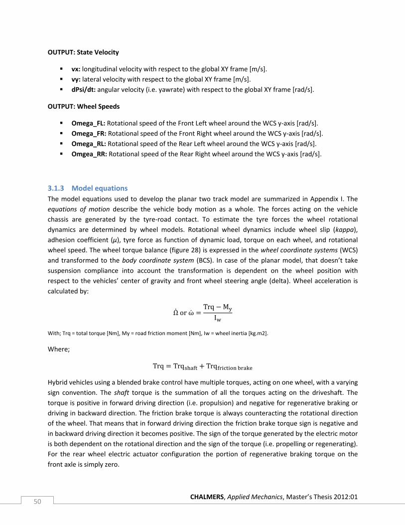
CHALMERS, Applied Mechanics, Master’s Thesis 2012:01 50
OUTPUT: State Velocity
vx: longitudinal velocity with respect to the global XY frame [m/s].
vy: lateral velocity with respect to the global XY frame [m/s].
dPsi/dt: angular velocity (i.e. yawrate) with respect to the global XY frame [rad/s].
OUTPUT: Wheel Speeds
Omega_FL: Rotational speed of the Front Left wheel around the WCS y-axis [rad/s].
Omega_FR: Rotational speed of the Front Right wheel around the WCS y-axis [rad/s].
Omega_RL: Rotational speed of the Rear Left wheel around the WCS y-axis [rad/s].
Omgea_RR: Rotational speed of the Rear Right wheel around the WCS y-axis [rad/s].
3.1.3 Model equations
The model equations used to develop the planar two track model are summarized in Appendix I. The
equations of motion describe the vehicle body motion as a whole. The forces acting on the vehicle
chassis are generated by the tyre-road contact. To estimate the tyre forces the wheel rotational
dynamics are determined by wheel models. Rotational wheel dynamics include wheel slip (kappa),
adhesion coefficient (µ), tyre force as function of dynamic load, torque on each wheel, and rotational
wheel speed. The wheel torque balance (figure 28) is expressed in the wheel coordinate systems (WCS)
and transformed to the body coordinate system (BCS). In case of the planar model, that doesn’t take
suspension compliance into account the transformation is dependent on the wheel position with
respect to the vehicles’ center of gravity and front wheel steering angle (delta). Wheel acceleration is
calculated by:
With; Trq = total torque [Nm], My = road friction moment [Nm], Iw = wheel inertia [kg.m2].
Where;
Hybrid vehicles using a blended brake control have multiple torques, acting on one wheel, with a varying
sign convention. The shaft torque is the summation of all the torques acting on the driveshaft. The
torque is positive in forward driving direction (i.e. propulsion) and negative for regenerative braking or
driving in backward direction. The friction brake torque is always counteracting the rotational direction
of the wheel. That means that in forward driving direction the friction brake torque sign is negative and
in backward driving direction it becomes positive. The sign of the torque generated by the electric motor
is both dependent on the rotational direction and the sign of the torque (i.e. propelling or regenerating).
For the rear wheel electric actuator configuration the portion of regenerative braking torque on the
front axle is simply zero.
CHALMERS, Applied Mechanics, Master’s Thesis 2012:01 51
Figure 28: Wheel torque balance, Source [2]
To avoid the vehicle model from starting to accelerate backwards three discrete states are defined.
State 1 is wheel rotation in positive direction, state 0 is no rotation (i.e. wheel lock or standstill) and
State -1 is wheel rotation in negative direction (figure 23). The friction brake torque flips sign for the
different states while the orientation of the shaft torque remains the same. This method makes sure,
that when the friction brake torque is larger than the tyre-road adhesion can support, the wheel
rotation doesn’t become negative, but will lock the wheel instead, even when the velocity of the vehicle
is non-zero. Figure 29 displays the embedded MATLAB function code, that is used in the torque balance
of the wheel models.
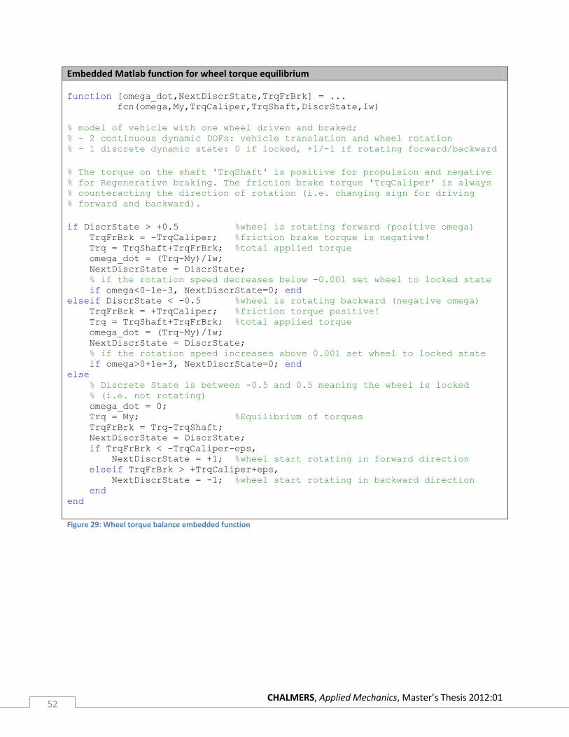
CHALMERS, Applied Mechanics, Master’s Thesis 2012:01 52
Embedded Matlab function for wheel torque equilibrium
function [omega_dot,NextDiscrState,TrqFrBrk] = ... fcn(omega,My,TrqCaliper,TrqShaft,DiscrState,Iw)
% model of vehicle with one wheel driven and braked; % - 2 continuous dynamic DOFs: vehicle translation and wheel rotation % - 1 discrete dynamic state: 0 if locked, +1/-1 if rotating forward/backward
% The torque on the shaft 'TrqShaft' is positive for propulsion and negative % for Regenerative braking. The friction brake torque 'TrqCaliper' is always % counteracting the direction of rotation (i.e. changing sign for driving % forward and backward).
if DiscrState > +0.5 %wheel is rotating forward (positive omega) TrqFrBrk = -TrqCaliper; %friction brake torque is negative! Trq = TrqShaft+TrqFrBrk; %total applied torque omega_dot = (Trq-My)/Iw; NextDiscrState = DiscrState; % if the rotation speed decreases below -0.001 set wheel to locked state if omega<0-1e-3, NextDiscrState=0; end elseif DiscrState < -0.5 %wheel is rotating backward (negative omega) TrqFrBrk = +TrqCaliper; %friction torque positive! Trq = TrqShaft+TrqFrBrk; %total applied torque omega_dot = (Trq-My)/Iw; NextDiscrState = DiscrState; % if the rotation speed increases above 0.001 set wheel to locked state if omega>0+1e-3, NextDiscrState=0; end else
% Discrete State is between -0.5 and 0.5 meaning the wheel is locked % (i.e. not rotating) omega_dot = 0; Trq = My; %Equilibrium of torques TrqFrBrk = Trq-TrqShaft; NextDiscrState = DiscrState; if TrqFrBrk < -TrqCaliper-eps, NextDiscrState = +1; %wheel start rotating in forward direction elseif TrqFrBrk > +TrqCaliper+eps, NextDiscrState = -1; %wheel start rotating in backward direction end end
Figure 29: Wheel torque balance embedded function
CHALMERS, Applied Mechanics, Master’s Thesis 2012:01 53
3.2 Tyre force estimators
The tyres, being the only connection between the vehicle body and the road, need a good
approximation of their behavior under driving- and environmental conditions. The tyres are the main
element in transmission of forces and therefore important for the study of limit handling. This paragraph
explains the development of the tyre force estimator as used in the wheel models.
Saab Automotive provided the EVBB project with an empirical tyre file from TNO Automotive. A so
called ‘tyre file’ lists the Magic Formula parameters, necessary for the usage of the MF-Tyre/MF-Swift
software. The free software application, including manuals, is available on the TNO website. Adding the
TNO Simulink block library to the MATLAB path enables the user to easily model tyres3.
The usage of TNO tyre blocks in the simulations resulted in unacceptably long simulation times. The aim
of the presented project, was to optimize the control by rapid simulation. Therefore, an alternative
approach is suggested; to estimate the tyre forces by means of look-up tables. Look-up tables are
commonly used in automotive electronics where, for example, injection duration and ignition timing are
stored on a memory called EPROM. The electronic control unit (ECU) can access these tables and read
the correct values for the engine operation. By the sensor outputs the ECU determines the position of
the correct actuation value (i.e. element in the look-up table). Although ‘exact’ values are not obtained,
the approach gives a sufficiently good approximation for control. By ‘pre-calculating’ the elements of a
look-up table, precious time is saved during operation.
The look-up tables used in the simulation are generated by an external program that calculates the tyre
forces for combined slip in several loop iterations. Roughly speaking the longitudinal- and lateral tyre
forces for combined slip are dependent on slip ratio (kappa), tyre slip angle (alpha), normal force (Fz)
and road adhesion coefficient (µ). The four independent variables result in the four dimensions of the
look-up table. For a comprehensive explanation of the full set of equations the writer would like to refer
to the book ‘Tire and Vehicle Dynamics’ by Hans B. Pacejka. The Magic Formula’s in general forms, used
for constructing the look-up tables, are;
0)arctan(arctancos)tan(,,, xHxxHxxxHxxxZX FSBSBESBCFF
)arctan(arctansin, 0 xxxxxxxxxx BBEBCDFwith
0)arctan(arctancos)tan(,,, yHyyHyyyHyyyZY FSBSBESBCFF
)arctan(arctansin, 0 yyyyyyyyyy BBEBCDFwith
The road adhesion can be differed by a scaling factor, λµ, (usually set equal to one) and will affect the
peak force (i.e. D parameter in Magic Formula and height of a tyre curve). Since the model is planar and
no chassis or suspension compliance is taken into account, no dynamic camber occurs. The static
3 Note: make sure to run MATLAB as administrator to add block library paths.
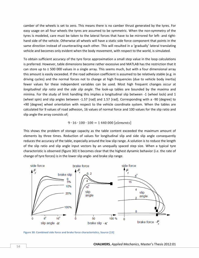
CHALMERS, Applied Mechanics, Master’s Thesis 2012:01 54
camber of the wheels is set to zero. This means there is no camber thrust generated by the tyres. For
easy usage on all four wheels the tyres are assumed to be symmetric. When the non-symmetry of the
tyres is modeled, care must be taken to the lateral forces that have to be mirrored for left- and right-
hand side of the vehicle. Otherwise all wheels will have a static side force component that points in the
same direction instead of counteracting each other. This will resulted in a ‘gradually’ lateral translating
vehicle and becomes only evident when the body movement, with respect to the world, is simulated.
To obtain sufficient accuracy of the tyre force approximation a small step value in the loop calculations
is preferred. However, table dimensions become rather excessive and MATLAB has the restriction that it
can store up to ± 500 000 values in a single array. This seems much, but with a four dimensional array
this amount is easily exceeded. If the road adhesion coefficient is assumed to be relatively stable (e.g. in
driving cycles) and the normal forces not to change at high frequencies (due to vehicle body inertia)
fewer values for these independent variables can be used. Most high frequent changes occur at
longitudinal slip ratio and the side slip angle. The look-up tables are bounded by the maxima and
minima. For the study of limit handling this implies a longitudinal slip between -1 (wheel lock) and 1
(wheel spin) and slip angles between -1.57 [rad] and 1.57 [rad]. Corresponding with a -90 [degree] to
+90 [degree] wheel orientation with respect to the vehicle coordinate system. When the tables are
calculated for 9 values of road adhesion, 16 values of normal force and 100 values for the slip ratio and
slip angle the array consists of;
This shows the problem of storage capacity as the table content exceeded the maximum amount of
elements by three times. Reduction of values for longitudinal slip and side slip angle consequently
reduces the accuracy of the table, especially around the low slip range. A solution is to reduce the length
of the slip ratio and slip angle input vectors by an unequally spaced step size. When a typical tyre
characteristic is observed (figure 30) it becomes clear that the highest dynamic behavior (i.e. the rate of
change of tyre forces) is in the lower slip angle- and brake slip range.
Figure 30: Combined side force and brake force characteristics, Source [13]
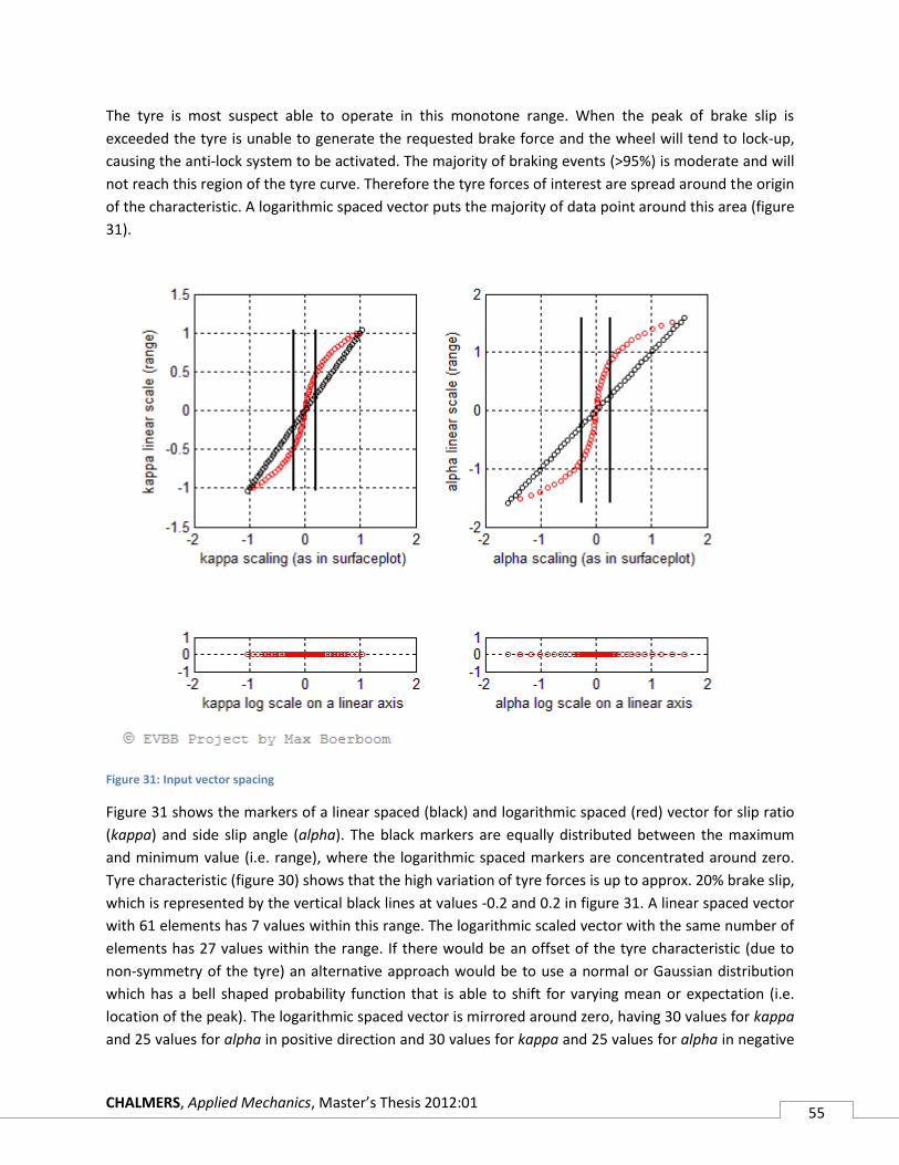
CHALMERS, Applied Mechanics, Master’s Thesis 2012:01 55
The tyre is most suspect able to operate in this monotone range. When the peak of brake slip is
exceeded the tyre is unable to generate the requested brake force and the wheel will tend to lock-up,
causing the anti-lock system to be activated. The majority of braking events (>95%) is moderate and will
not reach this region of the tyre curve. Therefore the tyre forces of interest are spread around the origin
of the characteristic. A logarithmic spaced vector puts the majority of data point around this area (figure
31).
Figure 31: Input vector spacing
Figure 31 shows the markers of a linear spaced (black) and logarithmic spaced (red) vector for slip ratio
(kappa) and side slip angle (alpha). The black markers are equally distributed between the maximum
and minimum value (i.e. range), where the logarithmic spaced markers are concentrated around zero.
Tyre characteristic (figure 30) shows that the high variation of tyre forces is up to approx. 20% brake slip,
which is represented by the vertical black lines at values -0.2 and 0.2 in figure 31. A linear spaced vector
with 61 elements has 7 values within this range. The logarithmic scaled vector with the same number of
elements has 27 values within the range. If there would be an offset of the tyre characteristic (due to
non-symmetry of the tyre) an alternative approach would be to use a normal or Gaussian distribution
which has a bell shaped probability function that is able to shift for varying mean or expectation (i.e.
location of the peak). The logarithmic spaced vector is mirrored around zero, having 30 values for kappa
and 25 values for alpha in positive direction and 30 values for kappa and 25 values for alpha in negative
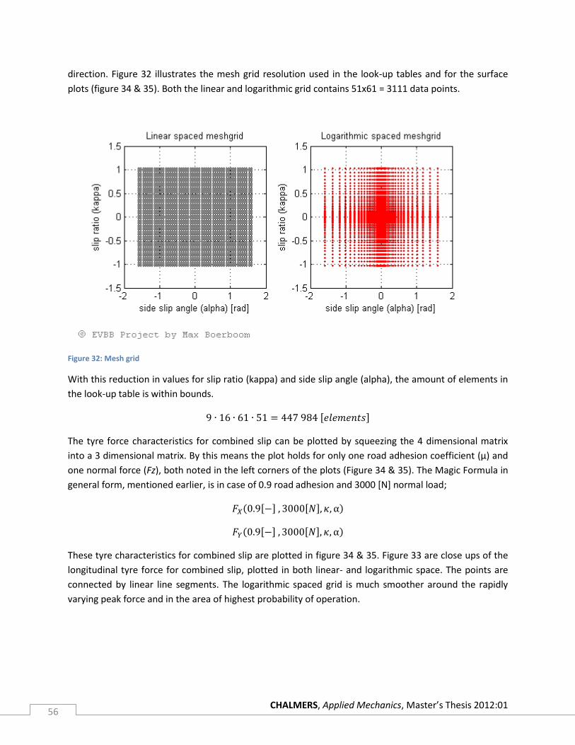
CHALMERS, Applied Mechanics, Master’s Thesis 2012:01 56
direction. Figure 32 illustrates the mesh grid resolution used in the look-up tables and for the surface
plots (figure 34 & 35). Both the linear and logarithmic grid contains 51x61 = 3111 data points.
Figure 32: Mesh grid
With this reduction in values for slip ratio (kappa) and side slip angle (alpha), the amount of elements in
the look-up table is within bounds.
The tyre force characteristics for combined slip can be plotted by squeezing the 4 dimensional matrix
into a 3 dimensional matrix. By this means the plot holds for only one road adhesion coefficient (µ) and
one normal force (Fz), both noted in the left corners of the plots (Figure 34 & 35). The Magic Formula in
general form, mentioned earlier, is in case of 0.9 road adhesion and 3000 [N] normal load;
These tyre characteristics for combined slip are plotted in figure 34 & 35. Figure 33 are close ups of the
longitudinal tyre force for combined slip, plotted in both linear- and logarithmic space. The points are
connected by linear line segments. The logarithmic spaced grid is much smoother around the rapidly
varying peak force and in the area of highest probability of operation.
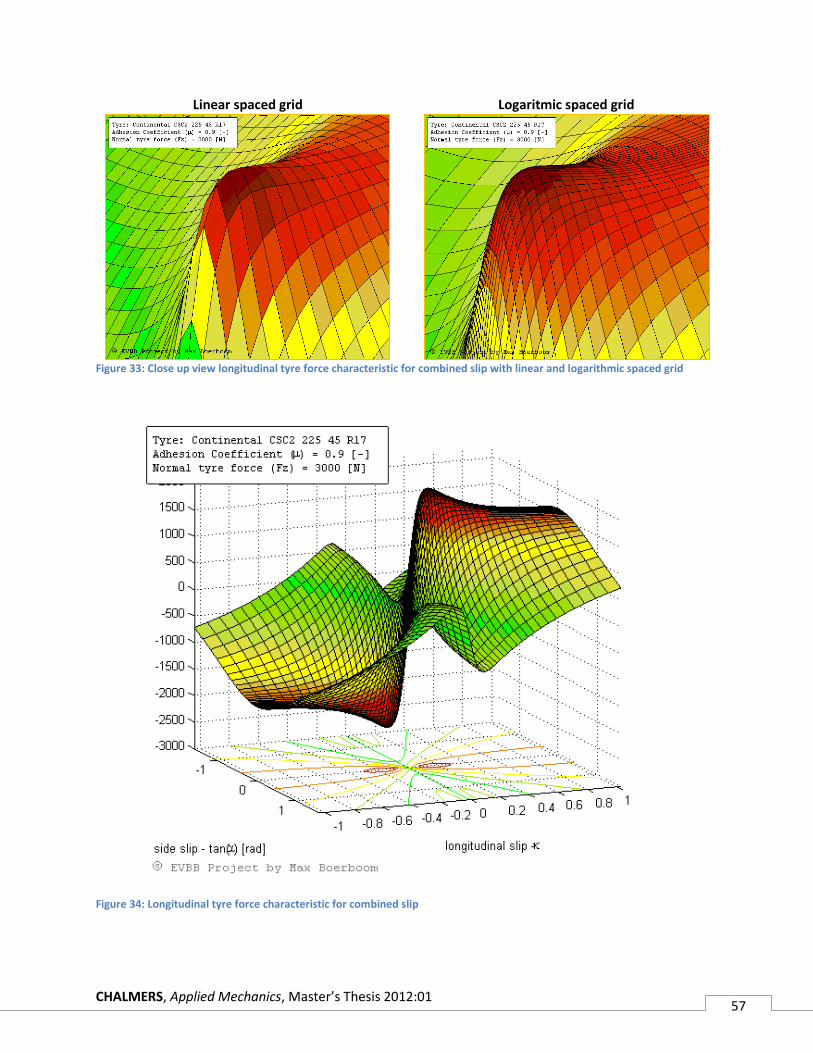
CHALMERS, Applied Mechanics, Master’s Thesis 2012:01 57
Linear spaced grid Logaritmic spaced grid
Figure 33: Close up view longitudinal tyre force characteristic for combined slip with linear and logarithmic spaced grid
Figure 34: Longitudinal tyre force characteristic for combined slip
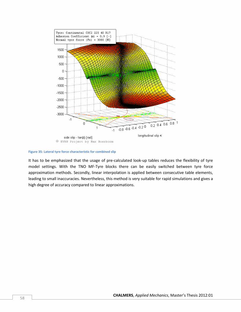
CHALMERS, Applied Mechanics, Master’s Thesis 2012:01 58
Figure 35: Lateral tyre force characteristic for combined slip
It has to be emphasized that the usage of pre-calculated look-up tables reduces the flexibility of tyre
model settings. With the TNO MF-Tyre blocks there can be easily switched between tyre force
approximation methods. Secondly, linear interpolation is applied between consecutive table elements,
leading to small inaccuracies. Nevertheless, this method is very suitable for rapid simulations and gives a
high degree of accuracy compared to linear approximations.
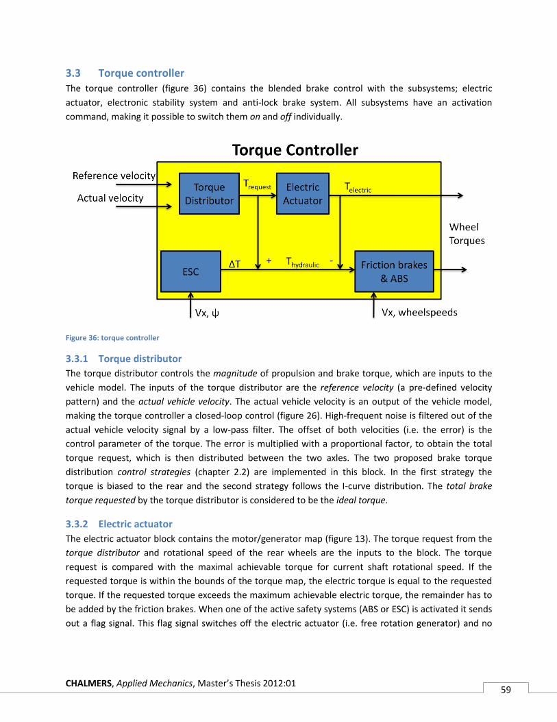
CHALMERS, Applied Mechanics, Master’s Thesis 2012:01 59
3.3 Torque controller
The torque controller (figure 36) contains the blended brake control with the subsystems; electric
actuator, electronic stability system and anti-lock brake system. All subsystems have an activation
command, making it possible to switch them on and off individually.
Figure 36: torque controller
3.3.1 Torque distributor
The torque distributor controls the magnitude of propulsion and brake torque, which are inputs to the
vehicle model. The inputs of the torque distributor are the reference velocity (a pre-defined velocity
pattern) and the actual vehicle velocity. The actual vehicle velocity is an output of the vehicle model,
making the torque controller a closed-loop control (figure 26). High-frequent noise is filtered out of the
actual vehicle velocity signal by a low-pass filter. The offset of both velocities (i.e. the error) is the
control parameter of the torque. The error is multiplied with a proportional factor, to obtain the total
torque request, which is then distributed between the two axles. The two proposed brake torque
distribution control strategies (chapter 2.2) are implemented in this block. In the first strategy the
torque is biased to the rear and the second strategy follows the I-curve distribution. The total brake
torque requested by the torque distributor is considered to be the ideal torque.
3.3.2 Electric actuator
The electric actuator block contains the motor/generator map (figure 13). The torque request from the
torque distributor and rotational speed of the rear wheels are the inputs to the block. The torque
request is compared with the maximal achievable torque for current shaft rotational speed. If the
requested torque is within the bounds of the torque map, the electric torque is equal to the requested
torque. If the requested torque exceeds the maximum achievable electric torque, the remainder has to
be added by the friction brakes. When one of the active safety systems (ABS or ESC) is activated it sends
out a flag signal. This flag signal switches off the electric actuator (i.e. free rotation generator) and no
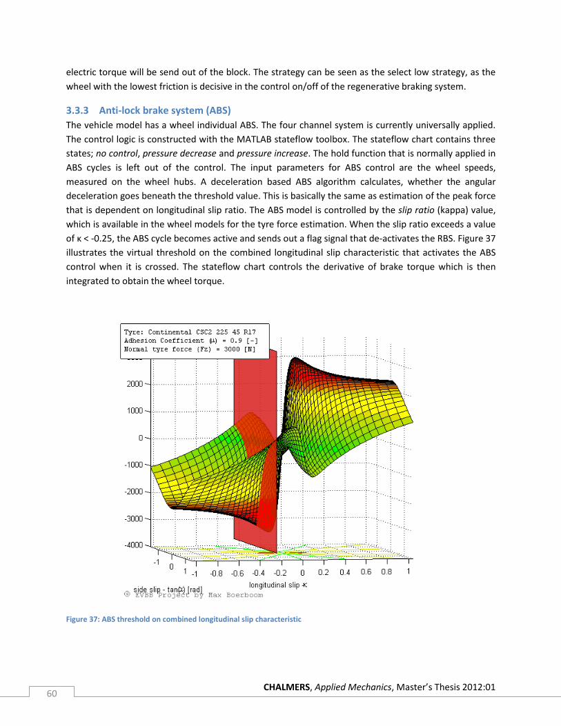
CHALMERS, Applied Mechanics, Master’s Thesis 2012:01 60
electric torque will be send out of the block. The strategy can be seen as the select low strategy, as the
wheel with the lowest friction is decisive in the control on/off of the regenerative braking system.
3.3.3 Anti-lock brake system (ABS)
The vehicle model has a wheel individual ABS. The four channel system is currently universally applied.
The control logic is constructed with the MATLAB stateflow toolbox. The stateflow chart contains three
states; no control, pressure decrease and pressure increase. The hold function that is normally applied in
ABS cycles is left out of the control. The input parameters for ABS control are the wheel speeds,
measured on the wheel hubs. A deceleration based ABS algorithm calculates, whether the angular
deceleration goes beneath the threshold value. This is basically the same as estimation of the peak force
that is dependent on longitudinal slip ratio. The ABS model is controlled by the slip ratio (kappa) value,
which is available in the wheel models for the tyre force estimation. When the slip ratio exceeds a value
of κ < -0.25, the ABS cycle becomes active and sends out a flag signal that de-activates the RBS. Figure 37
illustrates the virtual threshold on the combined longitudinal slip characteristic that activates the ABS
control when it is crossed. The stateflow chart controls the derivative of brake torque which is then
integrated to obtain the wheel torque.
Figure 37: ABS threshold on combined longitudinal slip characteristic
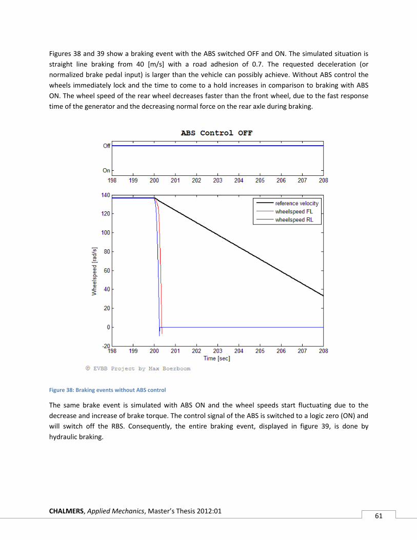
CHALMERS, Applied Mechanics, Master’s Thesis 2012:01 61
Figures 38 and 39 show a braking event with the ABS switched OFF and ON. The simulated situation is
straight line braking from 40 [m/s] with a road adhesion of 0.7. The requested deceleration (or
normalized brake pedal input) is larger than the vehicle can possibly achieve. Without ABS control the
wheels immediately lock and the time to come to a hold increases in comparison to braking with ABS
ON. The wheel speed of the rear wheel decreases faster than the front wheel, due to the fast response
time of the generator and the decreasing normal force on the rear axle during braking.
Figure 38: Braking events without ABS control
The same brake event is simulated with ABS ON and the wheel speeds start fluctuating due to the
decrease and increase of brake torque. The control signal of the ABS is switched to a logic zero (ON) and
will switch off the RBS. Consequently, the entire braking event, displayed in figure 39, is done by
hydraulic braking.
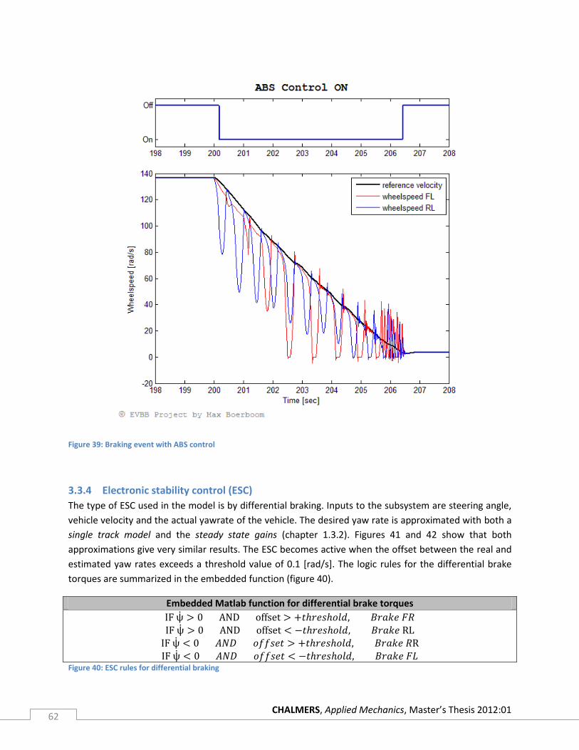
CHALMERS, Applied Mechanics, Master’s Thesis 2012:01 62
Figure 39: Braking event with ABS control
3.3.4 Electronic stability control (ESC)
The type of ESC used in the model is by differential braking. Inputs to the subsystem are steering angle,
vehicle velocity and the actual yawrate of the vehicle. The desired yaw rate is approximated with both a
single track model and the steady state gains (chapter 1.3.2). Figures 41 and 42 show that both
approximations give very similar results. The ESC becomes active when the offset between the real and
estimated yaw rates exceeds a threshold value of 0.1 [rad/s]. The logic rules for the differential brake
torques are summarized in the embedded function (figure 40).
Embedded Matlab function for differential brake torques
ψ ψ ψ ψ
Figure 40: ESC rules for differential braking
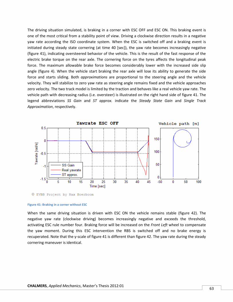
CHALMERS, Applied Mechanics, Master’s Thesis 2012:01 63
The driving situation simulated, is braking in a corner with ESC OFF and ESC ON. This braking event is
one of the most critical from a stability point of view. Driving a clockwise direction results in a negative
yaw rate according the ISO coordinate system. When the ESC is switched off and a braking event is
initiated during steady state cornering (at time 40 [sec]), the yaw rate becomes increasingly negative
(figure 41), indicating oversteered behavior of the vehicle. This is the result of the fast response of the
electric brake torque on the rear axle. The cornering force on the tyres affects the longitudinal peak
force. The maximum allowable brake force becomes considerably lower with the increased side slip
angle (figure 4). When the vehicle start braking the rear axle will lose its ability to generate the side
force and starts sliding. Both approximations are proportional to the steering angle and the vehicle
velocity. They will stabilize to zero yaw rate as steering angle remains fixed and the vehicle approaches
zero velocity. The two track model is limited by the traction and behaves like a real vehicle yaw rate. The
vehicle path with decreasing radius (i.e. oversteer) is illustrated on the right hand side of figure 41. The
legend abbreviations SS Gain and ST approx. indicate the Steady State Gain and Single Track
Approximation, respectively.
Figure 41: Braking in a corner without ESC
When the same driving situation is driven with ESC ON the vehicle remains stable (figure 42). The
negative yaw rate (clockwise driving) becomes increasingly negative and exceeds the threshold,
activating ESC rule number four. Braking force will be increased on the Front Left wheel to compensate
the yaw moment. During this ESC intervention the RBS is switched off and no brake energy is
recuperated. Note that the y-scale of figure 41 is different than figure 42. The yaw rate during the steady
cornering maneuver is identical.
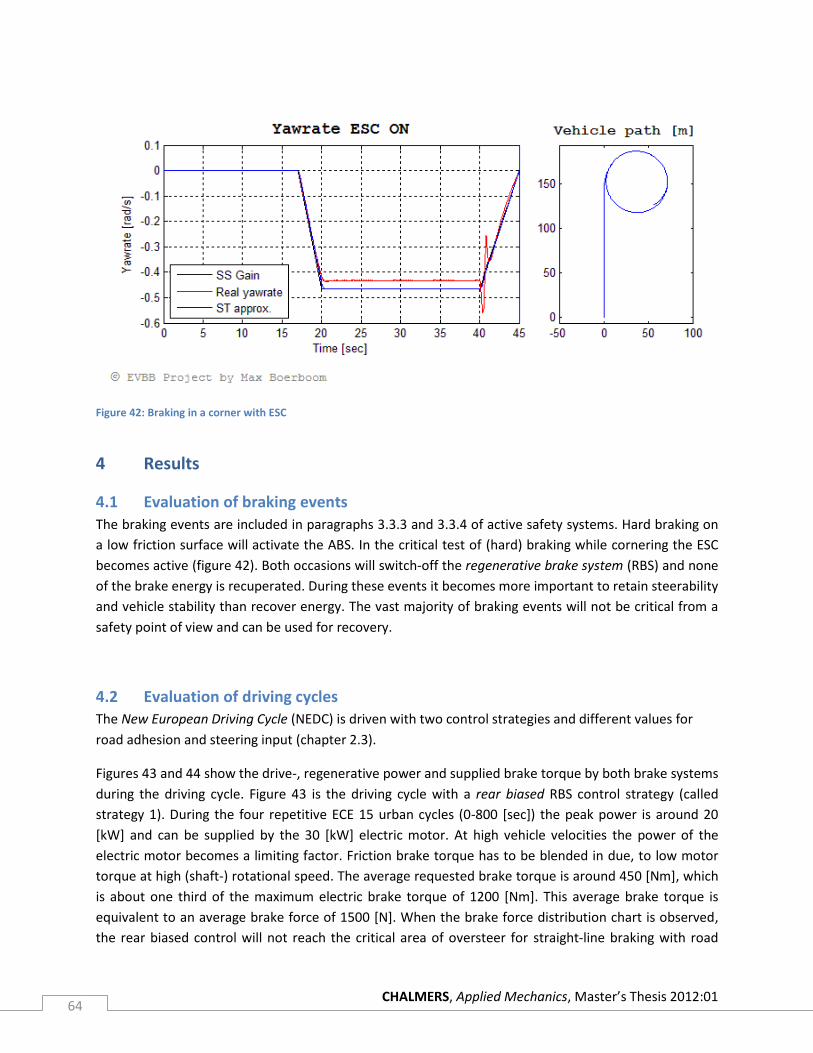
CHALMERS, Applied Mechanics, Master’s Thesis 2012:01 64
Figure 42: Braking in a corner with ESC
4 Results
4.1 Evaluation of braking events
The braking events are included in paragraphs 3.3.3 and 3.3.4 of active safety systems. Hard braking on
a low friction surface will activate the ABS. In the critical test of (hard) braking while cornering the ESC
becomes active (figure 42). Both occasions will switch-off the regenerative brake system (RBS) and none
of the brake energy is recuperated. During these events it becomes more important to retain steerability
and vehicle stability than recover energy. The vast majority of braking events will not be critical from a
safety point of view and can be used for recovery.
4.2 Evaluation of driving cycles
The New European Driving Cycle (NEDC) is driven with two control strategies and different values for
road adhesion and steering input (chapter 2.3).
Figures 43 and 44 show the drive-, regenerative power and supplied brake torque by both brake systems
during the driving cycle. Figure 43 is the driving cycle with a rear biased RBS control strategy (called
strategy 1). During the four repetitive ECE 15 urban cycles (0-800 [sec]) the peak power is around 20
[kW] and can be supplied by the 30 [kW] electric motor. At high vehicle velocities the power of the
electric motor becomes a limiting factor. Friction brake torque has to be blended in due, to low motor
torque at high (shaft-) rotational speed. The average requested brake torque is around 450 [Nm], which
is about one third of the maximum electric brake torque of 1200 [Nm]. This average brake torque is
equivalent to an average brake force of 1500 [N]. When the brake force distribution chart is observed,
the rear biased control will not reach the critical area of oversteer for straight-line braking with road

CHALMERS, Applied Mechanics, Master’s Thesis 2012:01 65
adhesions above 0.3 [µ]. The peaks on the brake torque graph (figures 43 & 44) are due to the
aggressive control of the torque distributor. A smoother response can be simulated, when the model is
extended with a driver model, that will apply the torque in a more natural way.
Figure 44 is the NEDC with the RBS control following the ideal brake force distribution curve (strategy 2).
The regenerative power (Regen power) is approximately half, compared to the rear biased strategy.
During I-curve braking the front brake force will be generated by the friction brakes and the rear part is
regenerative torque. The friction brakes will contribute to the total braking torque for every
deceleration, as can be seen from the bottom graph of figure 44, making the magnitude of regenerative
brake energy smaller compared to strategy 1 (Table 6). Both the velocity pattern and drive power of
figure 43 and 44 are identical.
Table 6 summarizes the total brake energy and regenerative brake energy for the NEDC under different
driving conditions and control strategies as proposed in chapter 2.3. Description of table columns:
Actuator: The electric motor (actuator) configuration (chapter 1.1.2 )
Regen Control: Control strategy of regenerative braking system (chapter 2.2)
Case No: Number of test case referring to the pie charts (figure 45 & 46)
Road adhesion: Road adhesion coefficient during entire simulation case.
Steering and lateral acc.: The front wheel steering angle during entire simulation case. If
steering is non-zero the steering input is proportional to the longitudinal velocity for a given
maximum lateral acceleration (equation 1.37).
Total brake energy: The total brake energy request for one simulation case, in ‘Mega Joule’. This
energy is required to track the velocity pattern of the driving cycle. The quantity is measured at
the ‘negative’ or brake torque output of the torque distributor.
Regen energy: The brake energy that is recuperated by the electric actuator, in ‘Mega Joule’.
Percent Regen w.r.t. Total brake energy: percentage of regenerative braking energy per
simulation case. The column presents the ratios of ‘Regen Energy’ and ‘Total Brake Energy’. This
means in case number 5 the regen percentage equals (1.431/1.528)*100 = 96%.
Percent Regen w.r.t. Theoretical maximum: percentage of regenerative brake energy with
respect to an idealized, theoretical maximum, case. The column presents the ratio of ‘Regen
energy’ and ‘Total brake energy’ for straight line braking on a high adhesion driving cycle. This
means that case number 5 the regen percentage equals (1.431/1.903)*100 = 76%.
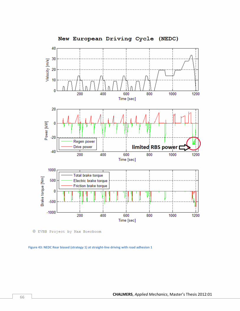
CHALMERS, Applied Mechanics, Master’s Thesis 2012:01 66
Figure 43: NEDC Rear biased (strategy 1) at straight-line driving with road adhesion 1
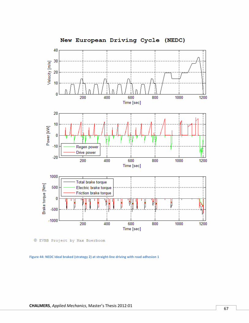
CHALMERS, Applied Mechanics, Master’s Thesis 2012:01 67
Figure 44: NEDC Ideal braked (strategy 2) at straight-line driving with road adhesion 1
CHALMERS, Applied Mechanics, Master’s Thesis 2012:01 68
The pie charts in figure45 show the portion of regenerative brake energy with respect to the total brake
energy. Figure 46 is the portion of regenerative brake energy with respect to the theoretical maximum.
The recuperated energy is the green fraction and energy dissipated by the friction brakes is the red
fraction of the pie. In the left column of both figures, control strategy 1 (i.e. bias all the brake torque to
the RBS) shows high portions of recuperation. Strategy 2 (right columns) follows the ideal brake
distribution curve and recuperates considerably lower amounts of energy.
The 90 percent regenerative brake energy for case 3 and 4 are due to shortage of electric power at high
vehicle velocities. In the last braking event the power of the electric motor is insufficient to meet the
brake torque request and a fraction of friction brake torque need to be added to fulfill the brake
request.
Cases 5, 6, 9 and 10 are braking in a corner with a steering input proportional to the vehicle velocity. The
average lateral acceleration at velocities above 10 [m/s] is about 3 [m/s2]. When the total brake energy
of those cycles is observed (table 6), the magnitude is less than for straight-line driving. This has to do
with a ‘resistive’ longitudinal component of the lateral tyre force during cornering. This longitudinal
component counteracts the driving direction (equation 1.38) reducing the required brake torque.
(1.38)
In driving case 6 for control strategy 1, the ESC is active for a duration of 100 [ms] in the last brake event
of the NEDC. The ESC flag will switch off the RBS, however, the short duration will hardly affect the
amount of regenerative brake energy.
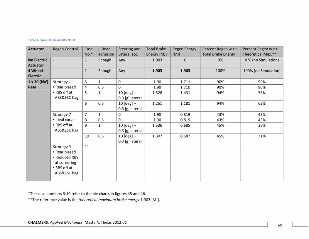
CHALMERS, Applied Mechanics, Master’s Thesis 2012:01 69
Table 6: Simulation results NEDC
Actuator Regen Control Case No.*
µ Road adhesion
Steering and Lateral acc.
Total Brake Energy [MJ]
Regen Energy [MJ]
Percent Regen w.r.t. Total Brake Energy
Percent Regen w.r.t. Theoretical Max.**
No Electric Actuator
- 1 Enough Any 1.903 0 0% 0 % (no Simulation)
4 Wheel Electric
- 2 Enough Any 1.903 1.903 100% 100% (no Simulation)
1 x 30 [kW] Rear
Strategy 1 ▪ Rear biased ▪ RBS off at ABS&ESC flag
3 1 0 1.90 1.711 90% 90%
4 0.5 0 1.90 1.710 90% 90%
5 1 10 [deg] – 0.3 [g] lateral
1.528 1.431 94% 76%
6 0.5 10 [deg] – 0.3 [g] lateral
1.251 1.181 94% 62%
Strategy 2 ▪ Ideal curve ▪ RBS off at ABS&ESC flag
7 1 0 1.90 0.819 43% 43%
8 0.5 0 1.90 0.819 43% 43%
9 1 10 [deg] – 0.3 [g] lateral
1.536 0.685 45% 36%
10 0.5 10 [deg] – 0.3 [g] lateral
1.307 0.587 45% 31%
Strategy 3 ▪ Rear biased ▪ Reduced RBS at cornering ▪ RBS off at ABS&ESC flag
11 - - - - - -
*The case numbers 3:10 refer to the pie charts in figures 45 and 46.
**The reference value is the theoretical maximum brake energy 1.903 [MJ].
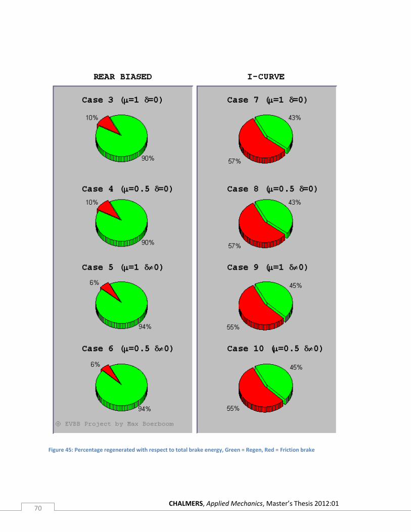
CHALMERS, Applied Mechanics, Master’s Thesis 2012:01 70
Figure 45: Percentage regenerated with respect to total brake energy, Green = Regen, Red = Friction brake
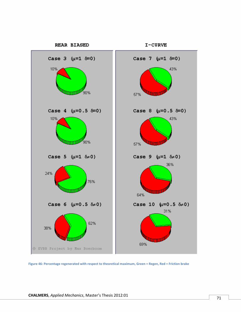
CHALMERS, Applied Mechanics, Master’s Thesis 2012:01 71
Figure 46: Percentage regenerated with respect to theoretical maximum, Green = Regen, Red = Friction brake
CHALMERS, Applied Mechanics, Master’s Thesis 2012:01 72
5 Conclusion The simulation results show that rear wheel regenerative braking is effective. The rear mounted
electric motor might seem to be in conflict with the requirement of vehicle stability, but the low
brake torques, at high speeds, generated by the 30 [kW] electric motor hardly affects the
stability of the vehicle. The control strategy to initially bias all the brake torque to the rear
shows best levels of energy recovery. This strategy could recover 90% of the brake energy in the
NEDC. Additional torque is blended in by an electro hydraulic brake-by-wire system, that
variably adds the difference between the requested- and electric brake torque.
On a mild cycle as the NEDC a 30 [kW] motor already shows power limitations, if controlled with
strategy 1 (rear biased torque). Controlling the regenerative brake system (RBS) according the I-
curve (control strategy 2) reduces this issue and makes the RBS suitable to recover energy over a
wider range of decelerations. Consequently, the portion of recovered energy with respect to
total brake energy will be reduced. However, normal driving conditions consist of decelerations
generally higher than 0.1 [g] and recovering a ‘steady’ 43% of all brake events might eventually
add up to a higher quantity of energy compared to strategy 1.
Although it is uncommon to run a driving cycle as the NEDC with a dynamic two track model it
proved to be stable. An interesting observation is that the required brake energy (i.e. the
integral of brake power) is less when the cycle is driven with a non-zero steering angle. An
explanation for this effect is, that the side forces on the (steered) front tyres generate a resistive
longitudinal force component during cornering.
Due to low rated power of the electric motor and the limitation to produce torque at zero
rotational speed, the ABS and ESC are maintained in their conventional way (i.e. hydraulic).
When an active safety system sends out a flag, the RBS is switched off. This approach works well
in the simulation, however, it should be investigated to what extend this will be noticeable to
the driver. A deceleration ‘gap’ must be avoided. A seamless transition from RBS to EHB is
necessary. This requires component response and more in-depth study about their control. An
alternative is, to study the possibility to use the electric motor for ABS control. The fast response
time could be suitable to vary the brake torque rather than the increase, decrease and hold of
brake torque. Secondly, the electric motor will have problems to lock a wheel, which is exactly
what ABS tries to avoid.
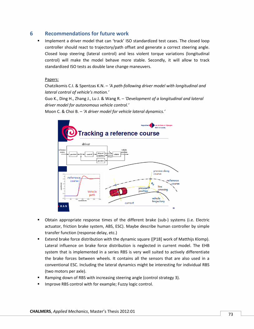
CHALMERS, Applied Mechanics, Master’s Thesis 2012:01 73
6 Recommendations for future work Implement a driver model that can ‘track’ ISO standardized test cases. The closed loop
controller should react to trajectory/path offset and generate a correct steering angle.
Closed loop steering (lateral control) and less violent torque variations (longitudinal
control) will make the model behave more stable. Secondly, it will allow to track
standardized ISO tests as double lane change maneuvers.
Papers:
Chatzikomis C.I. & Spentzas K.N. – ‘A path-following driver model with longitudinal and
lateral control of vehicle’s motion.’
Guo K., Ding H., Zhang J., Lu J. & Wang R. – ‘Development of a longitudinal and lateral
driver model for autonomous vehicle control.’
Moon C. & Choi B. – ‘A driver model for vehicle lateral dynamics.’
Obtain appropriate response times of the different brake (sub-) systems (i.e. Electric
actuator, friction brake system, ABS, ESC). Maybe describe human controller by simple
transfer function (response delay, etc.)
Extend brake force distribution with the dynamic square ([P18] work of Matthijs Klomp).
Lateral influence on brake force distribution is neglected in current model. The EHB
system that is implemented in a series RBS is very well suited to actively differentiate
the brake forces between wheels. It contains all the sensors that are also used in a
conventional ESC. Including the lateral dynamics might be interesting for individual RBS
(two motors per axle).
Ramping down of RBS with increasing steering angle (control strategy 3).
Improve RBS control with for example; Fuzzy logic control.
CHALMERS, Applied Mechanics, Master’s Thesis 2012:01 74
6 References
Books [1] M. Eshani, Y. Gao and A. Emadi (2010), “Modern Electric, Hybrid Electric and Fuel Cell
Vehicles Fundamentals, Theory and Design second edition,” Taylor and Francis Group,
ISBN 978-1-4200-5398-2.
[2] U. Kiencke and L. Nielsen (2005), “Automotive Control Systems For Engine, Driveline and
Vehicle, second edition,” Springer-Verlag Berlin Heidelberg, ISBN 3-540-23139-0.
[3] B. Heiβing, M. Ersoy (2011), “Chassis Handbook, Fundamentals, Driving Dynamics,
Components, Mechatronics, Perspectives,” Springer Fachmedien Wiesbaden GmbH
2011, ISBN 978-3-8348-0994-0.
[4] J. Larminie, J. Lowry (2003), “Electric Vehicle Technology Explained,” John Wiley & Sons
Ltd, The Atrium, Southern Gate, Chichester, West Sussex PO19 8SQ, England, ISBN 0-
470-85163-5.
[5] David A. Crolla (2009), “Automotive Engineering Powertrain, Chassis System and Vehicle
Body”, Elsevier Inc., ISBN 978-1-85617-577-7.
[6] John M. Miller (2008), “Propulsion Systems for Hybrid Vehicles”, The Institution of
Engineering and Technology, ISBN 978-0-86341-915-7.
[7] G. Genta and L. Morello (2009), “The Automotive Chassis, Volume 2: System Design”,
Springer Science and Business Media B.V., ISBN 978-1-4020-8673-1.
[8] H. Naunheimer, B. Bertsche, J. Ryborz and W. Novak (2010), “Automotive Transmissions
Fundamentals, Selection, Design and Application”, Springer-Verlag Berlin Heidelberg,
ISBN 978-3-642-16213-8.
[9] X. Zhang and C. Mi (2011), “Vehicle Power Management Modeling, Control and
Optimization” Springer-Verlag London Limited 2011, ISBN 978-0-85729-735-8.
[10] R. Hodkinson and J. Fenton (2001), “Lightweight Electric/ Hybrid Vehicle Design”,
Butterworth-Heinemann, ISBN 0-7506-5092-3.
[11] R. Rajamani (2006), “Vehicle Dynamics and Control”, Springer Science and Business
Media, Inc. ISBN 0-387-26396-9.
[12] G. Genta and L. Morello (2009), “The Automotive Chassis, Volume 1: Components
Design”, Springer Science and Business Media B.V., ISBN 978-1-4020-8674-8.
[13] H.B. Pacejka (2006), “Tire and Vehicle Dynamics, second edition”, Society of Automotive
Engineers, Inc., SAE ISBN 0-7680-1702-5.
CHALMERS, Applied Mechanics, Master’s Thesis 2012:01 75
Papers
[P1] S. Jang, H. Yeo, C. kim and H. Kim, “A study on Regenerative Braking for a Parallel Hybrid
Electric Vehicle” KSME International Journal, Vol. 15 No. 11, pp. 1490 ~ 1498, August
2001.
[P2] D. Peng, Y. Zhang, C.L. Yin and J.W. Zhang, “Combined Control of a Regenerative Braking
and Anti-lock Braking System for Hybrid Electric Vehicles”, International Journal of
Automotive Technology, Vol. 9, No. 6, pp. 749-757, May 2008.
[P3] M. Shang, L. Chu, J. Guo, Y. Fang and F. Zhou, “Braking Force Dynamic Coordinated
Control for Hybrid Electric Vehicles”, IEEE Advanced Computer Control (ICACC), 2010 2nd
International Conference, Vol. 4, pp. 411-416, June 2010.
[P4] J. Guo, J. Wang and B. Cao, “Study of Braking Force Distribution of Electric Vehicles”, IEEE
Power and Energy Engineering Conference, 2009. APPEEC 2009. Asia-Pacific, pp. 1-4,
May 2009.
[P5] M. Shang, L. Chu, J. Guo and Y. Fang, “Hydraulic Braking Force Compensation Control for
Hybrid Electric Vehicles”, IEEE International Conference on Computer, Mechatronics,
Control and Electronic Engineering (CMCE), Vol. 4, pp. 335-339, October 2010.
[P6] S. Zechang, L. Qinghe and L. Xidong, “Research on Electro-hydraulic Parallel Brake
System for Electric Vehicles”, Vehicular Electronics and Safety, 2006. ICVES 2006. IEEE
International Conference, pp. 376-379, June 2007.
[P7] Z. Tianjun and Z. Changfu, “Research on Electro-Hydraulic Brake System for Vehicle
Stability”, IEEE Industrial and Information Systems, 2009. IIS ’09. International
Conference, pp. 344-347, June 2009.
[P8] D. F. Reuter, E. Wayne Lloyd, J. W. Zehnder II and J. A. Elllot, “Hydraulic Design
Considerations for EHB Systems”, Delphi Corporation, SAE international DOI:
10.4271/2003-01-0324.
[P9] C. von Albrichsfeld and J. Karner, “Brake System for Hybrid Electric Vehicles”, SAE
International DOI: 10.4271/2009-01-1217, April 2009.
[P10] S. Hano and M. Hakiai, “New Challenges of Brake and Modulation Systems in Hybrid
Electric Vehicles (HEVs) and Electric Vehicles (EVs)”, SAE International DOI:
10.4271/2011-39-7210, May 2011.
[P11] E. Krueger, K. Kidston and A. Busack, “Reducing Disturbances Caused by Reductions in
Regenerative Braking Torque”, SAE International DOI: 10.4271/2011-01-0975, April
2011.
CHALMERS, Applied Mechanics, Master’s Thesis 2012:01 76
[P12] Y. Gao and M. Ehsani, “Electronic Braking System of EV and HEV – Integration of
Regenerative Braking, Automatic Braking Force Control And ABS”, SAE International DOI
10.4271/2001-01-2478.
[P13] L. Petruccelli, M. Velardocchia and A. Sorniotti, “Electro-Hydraulic Braking System
Modelling and Simulation”, SAE International DOI: 10.4271/2003-01-3336.
[P14] H. Yeo, C. Koo, W. Jung, D. Kim and J. S. Cheon, “Development of Smart Booster Brake
Systems for Regenerative Brake Cooperative Control”, SAE International DOI:
10.4271/2011-01-2356.
[P15] K. Beyer, E. Krueger and M. Sonnenberg, “Enhanced Vehicle Stability with Engine Drag
Control”, Delphi Automotive Systems, SAE International DOI: 10.4271/2002-01-1217.
[P16] J. Guo, J. Wang and B. Cao, “Regenerative Braking Strategy for Electric Vehicles” IEEE,
Publication no 978-1-4244-3504-3, Dec. 2008.
[P17] J. Fenzhu and L. Lijun, “Study on Braking Stability of Electro-mechanical Hybrid Braking
System in Electric vehicles Based on ECE Regulation” IEEE Publication bo 978-0-7695-
4350-5, 2011.
[P18] Klomp, M. and Thomson, R. (2011) ‘Infuence of front/rear drive force distribution on the
lateral grip and understeer of all-wheel drive vehicles’, Int. J. Vehicle Design, Vol. 56,
Nos. 1/2/3/4, pp.34–48.
Other
[A1] M. Duval-Destin, T. Kropf, V. Abadie, M. Fausten, “Impact of an Electric Powertrain on
the Braking System”, ATZ autotechnology, Volume 11, August 2011.
[A2] ‘MF-Tyre/MF-Swift 6.1.2.1 Help Manual’, TNO Automotive, The Netherlands, Document
revision September 2010.
[A3] J.P. Pauwelussen, ‘Advanced Vehicle Dynamics Master Automotive Engineering Lecture
notes’, revision 2009.
[A4] B. Vroemen, ‘Alternative Power Trains Lecture notes’ revision 2010.
[A5] ECE Regulation. Addendum 12-H: Regulation No. 13-H, Revision 2, October 2011.

CHALMERS, Applied Mechanics, Master’s Thesis 2012:01 77
APPENDIX
A1 Planar vehicle model equations
Appendix 1 summarizes the model equations used in the Matlab Simulink. The model can be
classified as a reduced nonlinear two track model. The vehicle coordinate systems are according
ISO 8855:1991 displayed in figure 47.
Figure 47: ISO coordinate system, Source [2]
Equations of motion
The equations of motion of a rigid body in plane with respect to the global coordinate system
(inertial frame) consist of two translations and a yaw torque balance around the vertical axis.
The rotation variable can be directly calculated in the undercarriage coordinate system since the
roll and pitch axis are assumed to lie at the road level.
ψ
ψ
ψ
Expanding the equations for a two-track model results in:
ψ
ψ
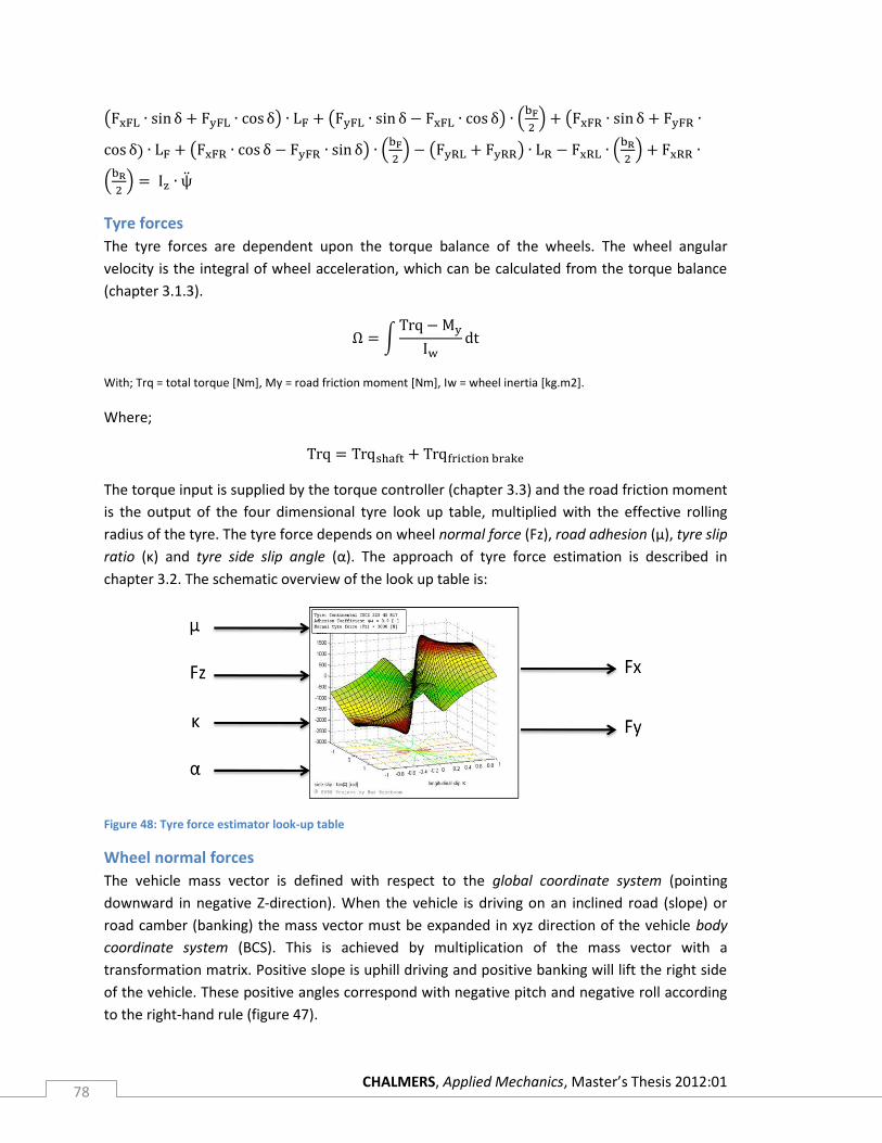
CHALMERS, Applied Mechanics, Master’s Thesis 2012:01 78
ψ
Tyre forces
The tyre forces are dependent upon the torque balance of the wheels. The wheel angular
velocity is the integral of wheel acceleration, which can be calculated from the torque balance
(chapter 3.1.3).
With; Trq = total torque [Nm], My = road friction moment [Nm], Iw = wheel inertia [kg.m2].
Where;
The torque input is supplied by the torque controller (chapter 3.3) and the road friction moment
is the output of the four dimensional tyre look up table, multiplied with the effective rolling
radius of the tyre. The tyre force depends on wheel normal force (Fz), road adhesion (µ), tyre slip
ratio (κ) and tyre side slip angle (α). The approach of tyre force estimation is described in
chapter 3.2. The schematic overview of the look up table is:
Figure 48: Tyre force estimator look-up table
Wheel normal forces
The vehicle mass vector is defined with respect to the global coordinate system (pointing
downward in negative Z-direction). When the vehicle is driving on an inclined road (slope) or
road camber (banking) the mass vector must be expanded in xyz direction of the vehicle body
coordinate system (BCS). This is achieved by multiplication of the mass vector with a
transformation matrix. Positive slope is uphill driving and positive banking will lift the right side
of the vehicle. These positive angles correspond with negative pitch and negative roll according
to the right-hand rule (figure 47).
CHALMERS, Applied Mechanics, Master’s Thesis 2012:01 79
Transformation matrices for relative yaw-pitch-roll motions between coordinate systems are:
A rotation about both the pitch and roll axis corresponds to the multiplication of the pitch and
roll transformation matrices and the gravity vector. The resulting vector is the gravity force
translated to the body coordinate system (BCS) and consists of the longitudinal resistance,
lateral thrust and vehicle normal force.
With; total vehicle mass m, gravitational acceleration g, pitch angle χ, roll angle ϕ.
The vertical forces or normal forces acting on the front and rear axle become:
With; wheelbase L, center of gravity height h, center of gravity to front and rear axle Lf and Lr, acceleration in
longitudinal direction ax.
Subsequently, the four wheel-ground contact point forces can be calculated when lateral
dynamics is included. This makes the normal forces dependent on:
Inclination angle (slope) effect
Corner camber or road banking angle
Longitudinal and lateral acceleration
CHALMERS, Applied Mechanics, Master’s Thesis 2012:01 80
With; wheelbase L, track width b, center of gravity height h, center of gravity to front and rear axle Lf and Lr,
accelerations in longitudinal and lateral directions ax and ay.
Wheel-ground contact point velocities (WGCPV)
To determine wheel slip the local velocities of the wheels need to be calculated. This is achieved
by transformation of the body coordinate system to the four wheel coordinate systems (tyre-
road contact points). It is assumed that variation of distance due to caster and pneumatic trail is
negligible. The magnitude of the distance from center of gravity to the front and rear wheels is:
The angle between this line and the symmetry axis of the vehicle is:
The wheel ground contact point velocities as vector notation are:
ψ ψ
ψ ψ
ψ ψ
ψ ψ
CHALMERS, Applied Mechanics, Master’s Thesis 2012:01 81
Tyre slip ratio and Besselink low speed damper
The longitudinal slip or slip ratio, denoted kappa, is defined as the ratio of longitudinal slip
velocity ‘Vsx’ and the forward speed of the wheel center ‘Vx’.
The slip ratio is bounded by -1 and 1, being wheel lock and wheel spin respectively. To limit the
slip ratio to a maximum of +1, the denominator is replaced by a relational operator.
As tyre forces don’t build up instantly the transient slip is introduced. The transient longitudinal
slip is determined by the restricted fully non-linear model [13]. This model is not sensitive to
wheel load variations, that affect the relaxation length, but therefore avoids an algebraic loop.
The first-order differential equation have been written in the form that makes it applicable for
simulations of stopping to and starting from zero velocity, by removing the longitudinal velocity
form the denominator.
Where the transient slip is defined;
So the equation can be written as:
The transient slip ratio κ’ is an input to the tyre force estimator. To avoid the high frequent
wind-up oscillations at the start and stop of a step changed propulsion torque, a Besselink low
speed damping is applied. This enables the transient model to operate near zero speed
conditions without heavy oscillations of the slip ratio. This damping is normally generated by the
tyre material [13]. The transient slip ratio becomes:
The damping factor kvlow is defined up to a certain threshold velocity. After exceeding this
threshold velocity the damping does not influence the transient slip ratio.
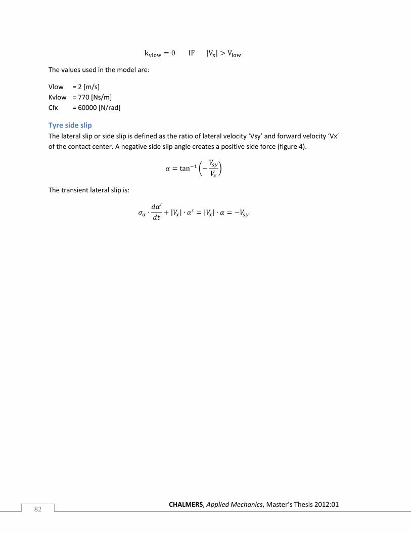
CHALMERS, Applied Mechanics, Master’s Thesis 2012:01 82
The values used in the model are:
Vlow = 2 [m/s]
Kvlow = 770 [Ns/m]
Cfκ = 60000 [N/rad]
Tyre side slip
The lateral slip or side slip is defined as the ratio of lateral velocity ‘Vsy’ and forward velocity ‘Vx’
of the contact center. A negative side slip angle creates a positive side force (figure 4).
The transient lateral slip is:
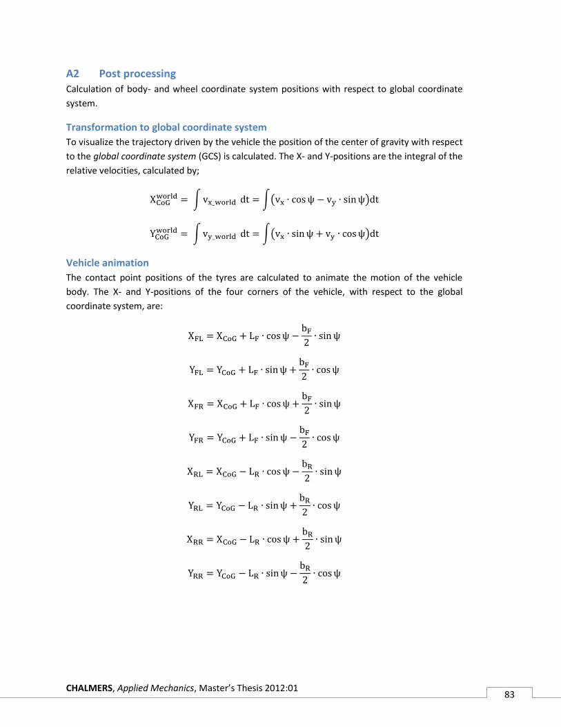
CHALMERS, Applied Mechanics, Master’s Thesis 2012:01 83
A2 Post processing
Calculation of body- and wheel coordinate system positions with respect to global coordinate
system.
Transformation to global coordinate system
To visualize the trajectory driven by the vehicle the position of the center of gravity with respect
to the global coordinate system (GCS) is calculated. The X- and Y-positions are the integral of the
relative velocities, calculated by;
ψ ψ
ψ ψ
Vehicle animation
The contact point positions of the tyres are calculated to animate the motion of the vehicle
body. The X- and Y-positions of the four corners of the vehicle, with respect to the global
coordinate system, are:
ψ ψ
ψ ψ
ψ ψ
ψ ψ
ψ ψ
ψ ψ
ψ ψ
ψ ψ