Embed Size (px)
Citation preview

Electric Energy StorageApplications and Effects on aMedium Voltage Grid
B.K. Gardiner
Masterof
ScienceTh
esis


Electric EnergyStorage
Applications and Effects on a Medium VoltageGrid
by
B.K. GardinerTo obtain the degree of
Master of Sciencein Electrical Engineering
at the Delft University of Technology,to be defended publicly on Monday September 12, 2016 at 02:00 PM.
Student number: 1505173Project duration: September 1, 2015 – July 1, 2016Supervisor: Prof. dr. ir. P. BauerThesis committee: Prof. dr. ir. P. Bauer, TU Delft
Dr. ir. L.M. Ramirez Elizondo, TU DelftDr. ir. J.L. Rueda Torres, TU DelftN.H. Baghina, M.Sc., Joulz Energy Solutions
Version 1.6August 31, 2016
An electronic version of this thesis is available at http://repository.tudelft.nl/.


Abstract
The importance of Electric Energy Storage has been recognized as early as the 1970’s. When inte-grated into electrical networks Electric Energy Storage has the potential of numerous technological andfinancial benefits. The importance of Electric Energy Storage is growing as more renewable energysources and higher consumer loads are added to existing networks. However, many of the beneficialeffects derived from Electric Energy Storage remain to be examined in detail. Therefore, it is the ob-jective of this thesis to examine several of these benefits, determine the methods by which they canbe incorporated into a Medium Voltage network and ascertain their precise effects on this network.
In this thesis three Electric Energy Storage benefits are reviewed and examined: peak shaving, fre-quency control and voltage control. Following this examination the technique of peak shaving has beenchosen to be further explored by subjecting it to various scenarios. Peak shaving has been selected asit appears to have the most potential benefits when applied to an electrical network. These benefitsare expected to be power supply increase, congestion relief, transmission upgrade deferral, and dis-tribution upgrade deferral. For the analysis process the Electric Energy Storage technology used is aBattery Energy Storage System. The Battery Energy Storage System provides for peak shaving on theMedium Voltage network.
In order to test five different scenarios an algorithm is developed using the DigSILENT Program-ming Language. This algorithm is tested using a simple reference network in order to determine ifit functions properly. After this, a test model based on an existing Medium Voltage network is createdusing PowerFactory on which the five different scenarios are tested. These scenarios are based onfuture growth of the network and an increase of the use of Photovoltaic and Electric Vehicles. Severalsimulations are run using these scenarios on different parts of the Medium Voltage network of Goeree-Overflakee to ascertain the effects of peak shaving on the network. In order to test the effects ondifferent network configurations three different actual network feeders are analyzed, two radial con-figured feeders and one meshed configured feeder.
From the results of this examination and research it is concluded that it is possible to use peak shavingto increase the power supply, reduce congestion, and defer transmission and distribution upgrades on aradial configured network. However, the process for meshed configuration simulation is not as straightforward. While the initial results are positive, additional research into the parameters of the simulationsoftware is required to provide a definite conclusion for meshed configurations. Finally, the addition ofElectric Vehicles creates complications in the operation of the Battery Energy Storage System. Severalsolutions are proposed to alleviate these complications. The addition of Photovoltaics partially removessome of these complications.
iii


Preface and Acknowledgments
For the last nine months I have been working on the analysis of Electric Energy Storage on a MediumVoltage grid at Joulz Energy Solutions for my master thesis project. This project was the final chapterin the journey towards my Master of Science degree in electrical engineering at the Delft University ofTechnology. There are many people who not only helped me bring this project to a successful conclu-sion but also aided and assisted me in my long journey towards my degree. I would like to take thisopportunity to acknowledge their contributions and thank them.
I would like to thank Joulz Energy Solutions for giving me this opportunity to work on an excitingand challenging project. In particular I would like to thank my daily supervisor, Nadina Baghina, forthe autonomy I was given to manage the project. I appreciate the many suggestions and frank andopen discussions we had. I would also like to thank Edward Coster for helping me with the initial stepsin exploring PowerFactory.
In addition, I would like to thank my supervisor Professor P. Bauer of the DC&E group for takingthe time and energy to supervise this thesis project and Seyedmahdi Izadkhast for his contribution tothe second half of the project.
There were a number of people who have helped me on my academic journey, and I cannot thinkof a better place than here to thank them. I would like to thank my family for the moral and financialsupport, everyone who helped review this thesis, my fellow student room inhabitants for moral supportand the lunch and coffee breaks, and finally you, the reader, for reading my thesis.
B.K. GardinerDelft, August 31, 2016
v

Contents
1 Introduction 11.1 Market Projections . . . . . . . . . . . . . . . . . . . . . . . . . . . . . . . . . . . . . . 11.2 Electric Energy Storage Technologies . . . . . . . . . . . . . . . . . . . . . . . . . . . 2
1.2.1 Mechanical energy storage technologies . . . . . . . . . . . . . . . . . . . . . 21.2.2 Electrical Energy Storage Technologies . . . . . . . . . . . . . . . . . . . . . . 31.2.3 Thermal energy storage technologies . . . . . . . . . . . . . . . . . . . . . . . 31.2.4 Chemical energy storage technologies . . . . . . . . . . . . . . . . . . . . . . 31.2.5 Electrochemical energy storage technologies . . . . . . . . . . . . . . . . . . 4
1.3 Electric Energy Storage Applications . . . . . . . . . . . . . . . . . . . . . . . . . . . 41.3.1 Electrical energy time-shift . . . . . . . . . . . . . . . . . . . . . . . . . . . . . 41.3.2 Power supply capacity . . . . . . . . . . . . . . . . . . . . . . . . . . . . . . . . 51.3.3 Load following. . . . . . . . . . . . . . . . . . . . . . . . . . . . . . . . . . . . . 51.3.4 Regulation . . . . . . . . . . . . . . . . . . . . . . . . . . . . . . . . . . . . . . . 51.3.5 Frequency response . . . . . . . . . . . . . . . . . . . . . . . . . . . . . . . . . 51.3.6 Spinning, non-spinning and supplemental reserve . . . . . . . . . . . . . . . 51.3.7 Voltage support . . . . . . . . . . . . . . . . . . . . . . . . . . . . . . . . . . . . 51.3.8 Black start. . . . . . . . . . . . . . . . . . . . . . . . . . . . . . . . . . . . . . . 61.3.9 Transmission congestion relief . . . . . . . . . . . . . . . . . . . . . . . . . . . 61.3.10Transmission upgrade deferral. . . . . . . . . . . . . . . . . . . . . . . . . . . 61.3.11Distribution upgrade deferral . . . . . . . . . . . . . . . . . . . . . . . . . . . 61.3.12Power quality management . . . . . . . . . . . . . . . . . . . . . . . . . . . . . 61.3.13Power reliability management . . . . . . . . . . . . . . . . . . . . . . . . . . . 61.3.14Retail electrical energy time-shift management . . . . . . . . . . . . . . . . . 61.3.15Demand charge management . . . . . . . . . . . . . . . . . . . . . . . . . . . 7
1.4 Thesis Outline . . . . . . . . . . . . . . . . . . . . . . . . . . . . . . . . . . . . . . . . 7
2 Research 92.1 Electric Energy Storage Systems. . . . . . . . . . . . . . . . . . . . . . . . . . . . . . 92.2 EESS Technology Choice . . . . . . . . . . . . . . . . . . . . . . . . . . . . . . . . . . 112.3 Research into Peak Shaving in Grids Using EES . . . . . . . . . . . . . . . . . . . . 122.4 Research into Frequency Control of Grids Using EES . . . . . . . . . . . . . . . . . 142.5 Research into Voltage Control of Grids Using EES . . . . . . . . . . . . . . . . . . . 152.6 Research Conclusions . . . . . . . . . . . . . . . . . . . . . . . . . . . . . . . . . . . . 172.7 Research Objective . . . . . . . . . . . . . . . . . . . . . . . . . . . . . . . . . . . . . . 182.8 Rules and Regulations with Regards to EES Grid Integration . . . . . . . . . . . . 18
3 Models and Simulation Scenarios 193.1 Reference Case . . . . . . . . . . . . . . . . . . . . . . . . . . . . . . . . . . . . . . . . 193.2 Real World Case . . . . . . . . . . . . . . . . . . . . . . . . . . . . . . . . . . . . . . . 19
3.2.1 Goeree-Overflakee . . . . . . . . . . . . . . . . . . . . . . . . . . . . . . . . . . 193.2.2 The Distribution System . . . . . . . . . . . . . . . . . . . . . . . . . . . . . . 20
3.3 BESS Model . . . . . . . . . . . . . . . . . . . . . . . . . . . . . . . . . . . . . . . . . . 203.4 Simulation Scenarios . . . . . . . . . . . . . . . . . . . . . . . . . . . . . . . . . . . . 223.5 Load Profiles. . . . . . . . . . . . . . . . . . . . . . . . . . . . . . . . . . . . . . . . . . 23
3.5.1 Regular Consumer Load Profiles . . . . . . . . . . . . . . . . . . . . . . . . . . 233.5.2 EV Consumption Profile . . . . . . . . . . . . . . . . . . . . . . . . . . . . . . . 243.5.3 PV Profile . . . . . . . . . . . . . . . . . . . . . . . . . . . . . . . . . . . . . . . 24
vii

viii Contents
4 Simulations and Results 274.1 Peak Shaving . . . . . . . . . . . . . . . . . . . . . . . . . . . . . . . . . . . . . . . . . 274.2 Reference Case Simulation . . . . . . . . . . . . . . . . . . . . . . . . . . . . . . . . . 294.3 Real World Case . . . . . . . . . . . . . . . . . . . . . . . . . . . . . . . . . . . . . . . 31
4.3.1 Scenario Current Consumer Size . . . . . . . . . . . . . . . . . . . . . . . . . 314.3.2 Scenario 120% Consumer Size. . . . . . . . . . . . . . . . . . . . . . . . . . . 334.3.3 Scenario 150% Consumer Size. . . . . . . . . . . . . . . . . . . . . . . . . . . 384.3.4 Scenario 200% Consumer Size. . . . . . . . . . . . . . . . . . . . . . . . . . . 43
4.4 Meshed Grid Configuration v. Radial Grid Configuration . . . . . . . . . . . . . . . 484.5 Peak Shaving with Electric Vehicles. . . . . . . . . . . . . . . . . . . . . . . . . . . . 48
4.5.1 EV Scenario at 120% Load . . . . . . . . . . . . . . . . . . . . . . . . . . . . . 484.5.2 EV Scenario at 150% Load . . . . . . . . . . . . . . . . . . . . . . . . . . . . . 48
4.6 Peak Shaving with Electric Vehicle and PV . . . . . . . . . . . . . . . . . . . . . . . 48
5 Conclusions and Recommendations 535.1 Conclusions . . . . . . . . . . . . . . . . . . . . . . . . . . . . . . . . . . . . . . . . . . 53
5.1.1 Conclusions of Reference Case Simulation. . . . . . . . . . . . . . . . . . . . 535.1.2 Conclusions of Feeder 103 . . . . . . . . . . . . . . . . . . . . . . . . . . . . . 535.1.3 Conclusions of Feeder 111 . . . . . . . . . . . . . . . . . . . . . . . . . . . . . 555.1.4 Conclusions of Feeder 204 . . . . . . . . . . . . . . . . . . . . . . . . . . . . . 55
5.2 Recommendations . . . . . . . . . . . . . . . . . . . . . . . . . . . . . . . . . . . . . . 56
A International Electrotechnical Commission Standards 57A.1 Fire Hazard Testing – IEC 60695-1-11:2010. . . . . . . . . . . . . . . . . . . . . . . 58A.2 Analysis Techniques for System Reliability – IEC 60812:2006 . . . . . . . . . . . . 58A.3 Fault Tree Analysis (FTA) – IEC 61025:2006. . . . . . . . . . . . . . . . . . . . . . . 58A.4 Protection from Electric Shock – IEC 61140:2002 . . . . . . . . . . . . . . . . . . . 59A.5 Batteries for Renewable Energy Storage – IEC 61427-1:2013. . . . . . . . . . . . . 59A.6 Functional Safety of Programmable Safety Related Systems IEC 61508 . . . . . . 59A.7 Safety of Lithium Batteries During Transport – IEC 62281:2013 . . . . . . . . . . 60A.8 Environmentally Conscious Design – IEC 62430:2009. . . . . . . . . . . . . . . . . 60A.9 Safety Requirements for Battery Installations – IEC 62485-2:2010 . . . . . . . . . 61
B DigSILENT PowerFactory Nine-bus System 63
C Single Line Diagrams 75
D Code 79
Bibliography 85
Glossary 89List of Acronyms . . . . . . . . . . . . . . . . . . . . . . . . . . . . . . . . . . . . . . . . . . 89List of Symbols . . . . . . . . . . . . . . . . . . . . . . . . . . . . . . . . . . . . . . . . . . . 90

“In the beginning the Universe was created. This has made a lot of people very angry andbeen widely regarded as a bad move.”
— Douglas Adams


1Introduction
The electricity supply grid is in fact a “just-in-time delivery system”, where variable consumer demandfor energy is translated into production, generation, at an energy source and transmitted via the sup-ply network. The dynamic fluctuations in demand generated over time by consumers must always bemet at a level that satisfies the customer’s requirements continuously. Failure to adequately supplyconsumer demand could result in damage to the stability and quality of the electrical power supply.As the world moves towards reliance on renewable sources of electrical energy the ability to provideElectric Energy Storage (EES) becomes of greater importance when providing for a continuous level ofelectrical supply identical to every change in consumers demand.
With a view towards this future in a dynamic and changing market, Joulz has entered into a jointproject with several other companies known as the GRIDSTOR project. The GRIDSTOR project deliver-able was a set of recommended practices for grid connected EES. These recommended practices canbe found in [1] and form the basis for the research element of this thesis.
1.1. Market ProjectionsIn the past most of electrical energy have been primarily produced using traditional forms, i.e. fos-sil fuel plants. These traditional forms of energy production can easily increase and decrease poweroutput to match the consumers demand. However, the world is moving towards renewable energysources which are reliant on external factors such as wind and sunlight. Renewable energy sourcessuch as wind and solar energy are relatively unpredictable when it comes to producing a constantsupply of energy. The reason for this is that they are subject to natural circumstances [2]. It is difficultto manage the raw production of fluctuating energy sources and thus harder to guaranty stability andquality of the generated energy. Another problem is that renewable energy sources are not usuallylocated in the place where the energy is consumed, therefor the transportations of energy via a grid isrequired to bring energy to the consumer. Failure of the grid due to congestion or any other reasonscan be devastating. These problems can be solved using EES; “by decoupling generation and load,grid energy storage would simplify the balancing act between electricity supply and demand, and onoverall grid power flow.” [3]
Currently the most common EES applications are: frequency control with over 300 projects world-wide, voltage support with over 200 projects worldwide, and peak shaving is found in at least 200projects globally [4]. The number of projects using these applications is only expected to grow as thebenefits of EES become more evident. A forecast provided by the Sandia National Laboratory (USA)projects that the overall market potential for EES will only grow in the future. When this growth iscoupled with the projected price reduction in EES predicted by the Boston Consulting Group, perfectconditions for growth and investments into new technologies are established [5]. This is only a logicalstep as the world moves towards renewable energy sources. Growing renewable energy sources suchas solar and wind energy cause fluctuations on the grid and EES is the most straight forward solutionfor this problem. Germany is a leading country when it comes to introducing renewable energy into
1

2 1. Introduction
the gird. The German energy market desires to increase its renewable energy production to 60% -80% of the total energy market [5]. Growth in EES will accompany this growth in renewable energyaccording to Siemens [6, 7].
The growth in Electric Vehicle (EV) is also an interesting trend. According to [8] the government inGermany expects the number of EVs to increase to one million by 2020. These vehicles can disrupt cur-rent networks by increasing the load when charging, but might be a solution when used as EES as well.
The main driver of the increase of EES is the move towards renewable energy sources in an effortto reduce CO2 emissions. This, in turn, calls for more research into EES in order to determine thetechnological and practical implications, thereby affecting new policies, standards, and developmentfor successful EES recommendations to accommodate this growth. [5]
1.2. Electric Energy Storage TechnologiesThe concept behind EES is straight forward: excess power generated from either renewable energysources or from traditional energy sources is stored for later use. The excess power can be storedusing different technologies i.e., mechanical, electrical, thermal, chemical, and electrochemical. Whenthe grid requires more power, the energy is transferred from the storage device back to the grid. Asmentioned above there are five major electric energy storage technologies. The following section willdiscuss the different technologies and provide examples of these technologies.
1.2.1. Mechanical energy storage technologiesMost common mechanical storage systems are pumped hydro, compressed air, and flywheel energystorage.
Pumped hydro storagePumped hydro storage currently represents nearly 99% of the world-wide installed electrical energystorage capacity. Energy is stored using pumped hydro by pumping water to a higher elevation. Whenenergy is needed the water flows down trough turbines that generated electricity. Typical dischargetimes can range from hours to days with an efficiency of 70% to 85%. This form of storage has along life cycle and the potential to store large amounts of energy. However, it requires a large area isneeded in order to do so.
Compressed air energy storageThe technique is relatively simple. Electricity is used to compress air which is then stored. When theenergy is required the compressed air is mixed with natural gas and burned in a turbine to createelectrical energy. This technique has a round trip efficiency of less than 50%, but is able to store largeamounts of energy.
Flywheel energy storageA flywheel stores energy as rotational energy using a rotating mass. The mass is kept rotating at aconstant speed. If the speed of the mass is increased, the amount of energy stored is also increased.By reducing the the speed of the mass energy can be extracted and used to create electrical energy.Advantages of the flywheel are: long life cycle and high power density. However, due to friction energyis lost during storage.
Mechanical storage has the advantage that, with certain technologies such as pumped hydro andcompressed air it can store energy for long periods of time without loss of energy. It can also be easilyscaled when large energy storage systems are required.
The disadvantage is that it always requires conversion from electrical power to mechanical power.This can never be completed with 100% efficiency. Energy is always lost when using mechanicalstorage. [5]

1.2. Electric Energy Storage Technologies 3
1.2.2. Electrical Energy Storage TechnologiesEnergy storage in the form of electrical energy is predominantly present in the form of super capacitorsand super conductors for storing electrical and magnetic energy.
Super capacitorsSuper capacitors, also known as double-layer capacitors are similar to regular capacitors in that theystore energy electro-statically between two electrodes. They differ in that they have an much largerstorage capability, unlimited cycle stability, and a higher power capability. However, they are not suitablefor storing energy over long periods of time, because of their self discharge rate.
Super conducting magnetic energy storageThis method of electrical energy storage, accumulates energy in a magnetic field using a super con-ducting coil. Feeding direct current into this coil a magnetic field is created. This technology has a veryfast response time, a high round-trip efficiency and a very high power output. The storage device doesconsume energy to keep the coil at its super conducting temperature. So that storing for long periodsof time costs energy. [9]
A big advantage of these technologies is that there is no conversion required which reduces energyloss and conversion is instantaneous.
There are disadvantages though. These forms of energy storage can only store energy for shortperiods of time and are difficult to scale.
1.2.3. Thermal energy storage technologiesThis form of energy storage is achieved by heating a substance, e.g., water or rocks. This heat isthen used at some later time to create electrical power. This form of energy storage can serve as anintermediate step in energy production. For example this technique is used in solar thermal energyproduction. The energy does not have to be delivered immediately to the grid, but can be saved fora time when demand is higher. Thermal storage can range from small water storage facilities to largeunderground bedrock chambers. Energy can be stored in this form for periods of hours, days, ormonths.
The downsides from these storage methods are that energy conversion time is high, there is a loss ofenergy in the conversion process and there is a loss in storage in the form of heat dissipation.
1.2.4. Chemical energy storage technologiesThis storage method is the practice of creating specific chemicals using electric energy which can thenlater be used to create electric energy. An example of this is electrolysis of water into oxygen andhydrogen. Electricity is used to split hydrogen and oxygen using a electrolyzer. The created hydrogenis then stored in pressurized containers until energy is needed. When the energy is needed it is trans-fered back in to electricity using a fuel cell. Advantages are storage longevity and low losses duringstorage.
Disadvantages include slow conversion times and energy losses during conversions.

4 1. Introduction
Figure 1.1: Gravimetric power and energy densities for different rechargeable batteries. [3]
1.2.5. Electrochemical energy storage technologiesElectrochemical storage has several features which make it a good option for EES. Some of thesefeatures are:
• pollution-free operation,
• high round-trip efficiency,
• flexible power and energy characteristics,
• long life cycle, and
• low maintenance.
However, they have one drawback: a high cost [3].
Many different battery types have been introduced in the past years, with Lithium-ion as one of themore recent technologies. According to Dunn et al. [3] the Lithium-ion Batteries (LIB) out preformsother technologies such as nickel (Ni)–metal hydride, Ni-cadmium (Cd), and lead (Pb)–acid by a factorof 2.5, as is shown in Figure 1.1. Lithium-ion also has high-output voltages, a high energy density, anda long life cylce which makes it a good candidate for EES.
1.3. Electric Energy Storage ApplicationsEES has multiple applications, and these abilities bring significant economic benefits for power con-sumers and distributing utilities [10]. This section will describe these applications and how their usecan benefit the electric network. A more detailed overview of all services can be found in [1] fromwhich this Section has been largely derived.
1.3.1. Electrical energy time-shiftElectrical energy time-shift is the practice of storing energy when prices are low and selling the powerback to the grid when prices are higher. For instance, energy can be bought when there is an abundanceof solar energy during the day and then be sold back at the end of the day when people are cominghome from work and there is no relatively inexpensive solar energy being produced. Electrical energytime-shift may be done by electric utilities in order to reduce cost or by storage owners to earn a profitfrom their storage capabilities. Electrical energy time-shift is a method of earning money rather thana method to ensure healthy grid operation.

1.3. Electric Energy Storage Applications 5
1.3.2. Power supply capacityEES can be used to delay the need for a new generation station by increasing the capacity of availableenergy during peak loads. EES stores energy during low loads and delivers energy during peak loadsrelieving the gird. This form of peak shaving lowers the overall strain on the network and increases theamount of energy available during peak times. Delaying the need for capital investment in new powerplants.
1.3.3. Load followingEES can be used in load following charges when there is an abundance of power and discharges whenthere is a shortage of power as compensation for the load variations. This can be accomplished byconventional power generation, but using EES has the benefits of operating with partial loads, and aquick response time, and can follow the dynamic ups and downs of load variation [11]. Load followingensures that the power demand of the loads is met. Energy needs to be bought from the the marketwhen charging and can be sold back when discharging. A high round-trip efficiency is important whenusing EES for this applications [1].
1.3.4. RegulationThis is power supply balancing of the momentary deviations of power flows in different control areasthat are caused by fluctuations in generation and load. EES is better suited for this application as ithas a faster reaction time than conventional systems, thus reducing wear and tear on generators bylimiting the need for them to rapidly change their power output [1].
1.3.5. Frequency responseRegulating the frequency in a network is important for the maintenance of power supply quality. Syn-thetic inertia is the change in power output proportional to the change in grid frequency. Many re-newable energy sources do not provide additional synthetic inertia. It is possible to use EES to addsynthetic inertia to the system. This technique can be used to compensate for frequency fluctuation.The most common method used to regulate frequency in the grid is by ramping up and down thepower output of the generators. This is not an instantaneous process and takes several minutes toaccomplish each movement. EES has a fast response time in the order of milliseconds. Because of thisthe frequency response of the system can be greatly reduced, smoothing the network frequency curveand thereby improving power quality delivery [5].
1.3.6. Spinning, non-spinning and supplemental reserveThis is an energy reserve technology that can be used in the case where a different form of generationcapacity becomes unavailable. This service ensures that the gird stays operational. This type of energyreserve can be divided into three elements:
• Spinning reserve is the first type of backup that is used when a power shortage occurs. It isconnected and synchronized with the grid and can compensate for generation or transmissionoutages.
• Non-spinning is the secondary backup after spinning reserve. It is grid connected, but not syn-chronized. It is usually available in less than 10 minutes after a problem has occurred.
• Supplemental reserve is the last backup and becomes available if both spinning and non-spinningreserves are not enough.
1.3.7. Voltage supportVoltage support is required to ensure that the grid voltage stays within its specified limits. This isaccomplished by using reactive power compensation. Reactive power compensation also improves thestability of the grid by increasing the maximum active power that can be transmitted. Traditionally,capacitors and inductors have been used to compensate for reactive power. In recent years self-commutated Pulse Width Modulation (PWM) converters are used to generate or absorb reactive power.Most types of EES use a PWM to convert from AC to DC and vice versa. Here the PWM is used to serveas a source or sink for the reactive power as these systems have [11].
6 1. Introduction
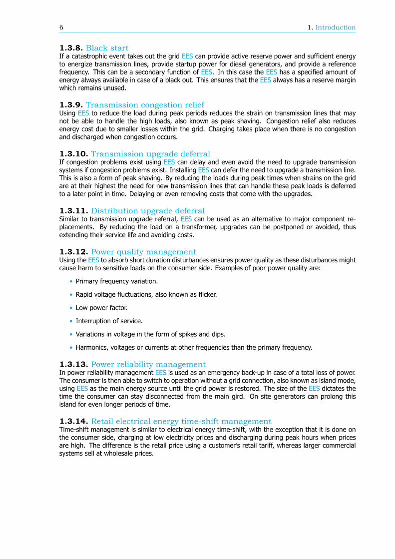
1.3.8. Black startIf a catastrophic event takes out the grid EES can provide active reserve power and sufficient energyto energize transmission lines, provide startup power for diesel generators, and provide a referencefrequency. This can be a secondary function of EES. In this case the EES has a specified amount ofenergy always available in case of a black out. This ensures that the EES always has a reserve marginwhich remains unused.
1.3.9. Transmission congestion reliefUsing EES to reduce the load during peak periods reduces the strain on transmission lines that maynot be able to handle the high loads, also known as peak shaving. Congestion relief also reducesenergy cost due to smaller losses within the grid. Charging takes place when there is no congestionand discharged when congestion occurs.
1.3.10. Transmission upgrade deferralIf congestion problems exist using EES can delay and even avoid the need to upgrade transmissionsystems if congestion problems exist. Installing EES can defer the need to upgrade a transmission line.This is also a form of peak shaving. By reducing the loads during peak times when strains on the gridare at their highest the need for new transmission lines that can handle these peak loads is deferredto a later point in time. Delaying or even removing costs that come with the upgrades.
1.3.11. Distribution upgrade deferralSimilar to transmission upgrade referral, EES can be used as an alternative to major component re-placements. By reducing the load on a transformer, upgrades can be postponed or avoided, thusextending their service life and avoiding costs.
1.3.12. Power quality managementUsing the EES to absorb short duration disturbances ensures power quality as these disturbances mightcause harm to sensitive loads on the consumer side. Examples of poor power quality are:
• Primary frequency variation.
• Rapid voltage fluctuations, also known as flicker.
• Low power factor.
• Interruption of service.
• Variations in voltage in the form of spikes and dips.
• Harmonics, voltages or currents at other frequencies than the primary frequency.
1.3.13. Power reliability managementIn power reliability management EES is used as an emergency back-up in case of a total loss of power.The consumer is then able to switch to operation without a grid connection, also known as island mode,using EES as the main energy source until the grid power is restored. The size of the EES dictates thetime the consumer can stay disconnected from the main gird. On site generators can prolong thisisland for even longer periods of time.
1.3.14. Retail electrical energy time-shift managementTime-shift management is similar to electrical energy time-shift, with the exception that it is done onthe consumer side, charging at low electricity prices and discharging during peak hours when pricesare high. The difference is the retail price using a customer’s retail tariff, whereas larger commercialsystems sell at wholesale prices.

1.4. Thesis Outline 7
1.3.15. Demand charge managementDemand charge management is a process of saving energy when the energy price is low and using itwhen it is needed and the prices are higher. This lowers the energy usage during peak hours and savesmoney for the consumer. In contrast to time-shift management, the moment of charge and dischargeis solidly based on the price of energy and not on the power output.
1.4. Thesis OutlineAs can be observed in Section 1.3, the applications for EES are numerous. While it is quite possibleto explore and evaluate each of these applications, the focus of this thesis is restricted to researchinto those applications which are most relevant for Joulz’s business model. A cursory examination ofthe sixteen applications set out above reveals that many have similar overlapping methodologies andeffects on the grid. For example, power supply capacity, transmission congestion relief, transmissionupgrade deferral, and distribution upgrade deferral can all be incorporated into the grid through theuse of peak shaving. These applications are also an interesting research subject for Joulz because theirimplementation is anticipated to prolong the life of the grid and its connected elements and to reducecosts and increase available power. For Joulz as well as the writer, it is a logical choice to include theseapplications in the thesis research.
In addition to these applications, there is also an interest in researching the frequency response andvoltage support applications as they result in higher power quality for consumers. Power quality is ofprimary importance to Joulz’s customer satisfactions goals. These applications will also form part theresearch.
In Chapter 2 the research and its requirements are set out. The purpose of the research is to de-termine what effects the different applications have on a grid, and to determine if these are positivedesirable effects for the grid under examination in this thesis. With the results of this research it ispossible to determine which applications are to be further examined and to predict what effects theseapplications will have on the gird.
In Chapter 3 the case models are described and their implementation discussed. These models will beused to run different scenarios through simulation and to examine the effects of the proposed method-ologies on these models. Each of the individual scenarios are presented and evaluated in this chapter.
In Chapter 4 the different methodologies are examined and the results obtained from the simulationsusing each of the models and the various scenarios are discussed. From these results it is possible todetermine the possible need for adjustments in the methodology.
Finally, in Chapter 5 the results of the simulations are examined, discussed and conclusions are drawnbased on the findings. Based on these conclusions recommendations are provided for future researchwork.


2Research
As early as 1970 the importance of EES had been noted [12]. Chen, et al. concluded in their article:“EES is urgently needed by the conventional electricity generation industry, DER and intermittent re-newable energy supply systems. By using EES, challenges faced by the power industry can be greatlyreduced. EESs have numerous applications covering a wide spectrum, ranging from large-scale gener-ation and transmission-related systems, to distribution network and even customer/end-user sites. TheEES technologies provide three primary functions of energy management, bridging power and powerquality and reliability.” [13]
EES has been proven to have a number of specific economic benefits. The most important of theseare:
• cutting costs for consumers,
• stabilizing the market from speculation,
• more efficient use of renewable energy,
• reducing grid congestion, and
• the cost of energy storage components is relatively inexpensive.
These and additional economic benefits are further detailed in [14–17]. It is clear that there is a grow-ing need for EES from both an economic, and a technological perspective. Therefore, the importanceof improving EES technologies cannot be overlooked.
This chapter focuses on research into peak shaving, voltage control and frequency control applicationsand their respective effects on the grid. From this research it is possible to determine their suspectedinfluences on the grid and their relevance for this thesis research topic. In addition to examination ofthe applications, this thesis will examine the existing regulatory framework governing the integrationof EES into the Dutch electricity grid. At present EES is not wildly implemented. It is of benefit to havean overview of the existing regulations pertaining to integration in order to discover potential missingregulations that might improve integration in the future.
2.1. Electric Energy Storage SystemsTo use EES it must form an integrated part of the grid. In order to connect the EES to the gird, servercomponents are required. The combination of these components with the EES component is called anEESS. Figure 2.1 illustrates in a schematic diagram of an EESS. This generic schematic is applicable toeach of the different EES technologies.
An EESS consists of several parts. The first is the EES. This can be any of the above mentionedenergy storage technologies.
9

10 2. Research
The second component is a Power Conversion System (PCS) to transform the energy from the ACgrid to the energy required by the EES and vice versa e.g., transformation from AC to mechanicalmotion for mechanical storage or transformation from AC to DC for battery storage. In most casesthere is a transformer placed between the grid and the PCS.
The third EES component is the monitoring system for the storage element. This can either bethe Storage Management System (SMS) or the Battery Management System (BMS) for batteries. TheSMS reads out all the relevant data from the physical EES component and ensures that the system isfunctioning within its operating limits. The SMS also checks if the requested power can be deliveredby the system in its current state.
The final component is the Energy Management System (EMS) which regulates the state of theEESS. EES has three different states: charged, idles or discharged. To function properly most EESSalso require an auxiliary system to function properly. For example, batteries might require cooling anda fly wheel will require a vacuum pump. This auxiliary system is monitored by the SMS. [1]
Transformer
PowerConversionSystem(PCS)
PhysicalEES device
Storage Manage-ment System (SMS)(low-level controls)
Energy Manage-ment System (EMS)(high-level controls)
Periphery /auxiliaries
Power
PowerPower
Power to be transferred
EES stateRequired power Monitoring &control
Conditioning
Measurements
Data
Figure 2.1: Schematic top-level drawing of an EESS. [1]

2.2. EESS Technology Choice 11
Table 2.1: Technology comparison of potential batteries for EES. [13, 18]
type specific energy (Wh/kg) discharge time storage duration energy efficiency (%)
LAB 25–40 up to 8 h minutes–days 50–75NCB 30–45 up to 4 h minutes–days 55–70VRB 10–20 4–12 h hours–months 65–80Na-S 150–240 4–8 h seconds–hours 75–90C-LC (LIB) 155 up to 4 h minutes–days 94–99LT-LFP (LIB) 50–70 up to 4 h minutes–days 94–99
2.2. EESS Technology ChoiceElectrochemical storage technologies have many advantages when it comes to frequency control andvoltage control [3, 13, 16, 18–20]. Most of these advantages have already addressed in Subsection 1.2.5.
Battery Energy Storage System (BESS) offers a financial benefit over Compressed Air Energy Stor-age (CAES) and Pumped Hydro Storage (PHS), due to their capital costs and site requirements [21].BESS has become a popular tool for energy storage because of its fast ramping time, cost of operation,and relatively low capital investment. As a consequence, it is more suitable for peak shaving then otherEES methods. Using these arguments as a basis it can be concluded that a BESS is the best choice forfrequency regulation, voltage regulation, and peak shaving.
There are several different options when it comes to the selection of battery technology.
Lead-acid BatteriesLead-acid Batteries (LAB) are composed of a positive lead dioxide (PbO2) electrode and a negativeelectrode of lead (Pb). These two electrodes are separated by a micro-porous material. When theelectrodes are immersed into sulfuric acid an open circuit potential of 3 V is created. When the circuitis closed the battery discharges its stored energy. The lead dioxide is reduced to lead oxide, this reactswith the acid to form lead sulfate. The battery can be charged which reverses this process. [10]
Nickel-cadmium BatteriesNickel-cadmium Batteries (NCB) have a positive electrode made of nickel hydroxide (Ni(OH)2) and anelectrolyte of potassium hydroxide (KOH) with some lithium hydroxide (LiOH). The negative electrodeis made of cadmium hydroxide (Cd(OH)2). The rated open circuit voltage for NCB is 1.2 V. [20]
All-vanadium Redox Flow BatteriesAll-vanadium Redox Flow Batteries (VRB) are a type of Redox Flow Batteries (RFB). This type of batterystores energy in two soluble redox couples contained in external electrolyte tanks. Liquid electrolytesare pumped from these tanks to flow through the electrodes where the electrical energy is convertedinto chemical energy or vise versa. These types of batteries are more like fuel cells then traditionalbatteries. VRB have a complex operation and is further detailed in [18].
Sodium-sulfur BatteriesSodium-sulfur Batteries (Na-S) are high-temperature batteries, meaning they operate at temperaturesof 270 to 350 ∘C. The positive electrode is formed from sulfur (S) and the negative electrode fromsodium (Na). Due to the hight temperature both electrodes are liquid. The 𝛽-alumina, which is usedas conducting membrane, is also more conductive at these high temperatures. Discharging the batteryresults in the oxidation of the sodium which travels trough the electrolyte and reacts with the sulfur.The opposite happens when the battery is charged. The resulting open circuit voltage is 2.08 V. [3]
Lithium-ion BatteriesLi-ion Batteries of C anode and LiCoO2 cathode (C-LC) and Li-ion Batteries of Li4Ti5O12 anode andLiFePO4 cathode (LT-LFP) are both types of Lithium-ion Batteries (LIB). These batteries store energyin electrodes made of lithium (Li). During discharge lithium ions (Li+) transfer through the electrolyteto the other electrode. The electrolyte can be a liquid, a gel or a solid depending on the type of battery.

12 2. Research
In Table 2.1 battery characteristics are shown that have an importance in these applications. Ac-cording to [3, 13, 18] LIB technology is a good contender when it comes to frequency regulation andenergy throughput balancing due to its high efficiency, fast discharge time and its ability to store energyfor longer durations. It also has a high specific energy implying that fewer batteries are needed forstoring the same amount of energy compared to lead-acid batteries, for example. For these reasonsLIB is the best choice.
2.3. Research into Peak Shaving in Grids Using EESPeak shaving is a process of reducing load when the load in the network reaches a specified limit,referred to as peak loads, power from an alternate source. This alternate energy source is usually alocal EESS. The energy this EESS produces is saved during low loads, when the strain on the networkis at a minimum. Peak shaving is said to have several benefits:
• reduction of power supply capacity,
• transmission and distribution upgrade deferral, and
• congestion relief.
These effects can potentially lower costs for both consumer and supplier, increase the efficiency ofrenewable energy sources, and prolong the life of network elements.
Peak shaving is not to be confused with load shifting. In load shifting a load over a certain timeperiod is shifted to a different time period using EES, much in the same way it is done with peak shav-ing. The key difference is when peak shaving is the load that is used to determine when to charge anddischarge the EESS and with load shifting it is the time period that is used.
Currently more than 200 peak shaving projects exists world wide. Its application is becoming moreimportant with the increase of renewable energy. In a study by Chua et al. [22] power consumptionwas reduced. This is clearly visible in Figure 2.2. In Table 2.2 the energy and power values of this caseare given for with and without peak shaving. The consumed energy is the same for both cases, butthe maximum requested power is much lower when utilizing peak shaving than when not.
In [23] Leadbetter and Swan ran simulations with an EESS close to the consumer using realistic 5-minute time-step load profiles in order to assess the battery size when reducing the peak in electricitydemand. Their results suggest a 5 kWh/2.6 kW for low energy usage homes and 22 kWh/5.2 kW forhigh energy usage homes.
In [24] Lu et al. analyze the optimal sizing and control of a BESS for peak shaving. They foundthat optimizing control methods result in improved peak load shaving performances using limited BESScapacity.
In [21] Rahimi et al. proposes a simple yet effective peak shaving algorithm. This method showspositive results utilizing only a simple algorithm for peak shaving. From this article it would appear thatcomplex control methods are not a necessity for peak shaving.

2.3. Research into Peak Shaving in Grids Using EES 13
Table 2.2: Power usage [22]
Actual
Power usage 27,163 kWhMaximum demand 152.4 kW
Peak shaving
Power usage 27.163 kWhMaximum demand 87.42 kW
Figure 2.2: Power consumption. [22]

14 2. Research
2.4. Research into Frequency Control of Grids Using EESFrequency control is important in electrical power girds in order to keep power generation stable. Fre-quency control entails the maintenance of a steady minimum modulation within the power grid whenthe steady state in disturbed. A deviation in frequency occurs when there is an imbalance betweengenerated power and load side power demand. There are two forms of frequency control: PrimaryFrequency Control (PFC) and Secondary Frequency Control (SFC). PFC works dynamically using afeedback regulatory system. It reacts relatively fast (within seconds) to frequency changes within thegrid. On the other hand, SFC regulates the gird frequency close to its nominal value by adjusting allthe generators connected to the frequency control system. SFC response times are higher than PFC,usually minutes. EES can both be used for PFC and SFC.
As early as 1993 research was already well underway into frequency regulation using EES. In [25]a BESS able to supply 30 MW for 15 minutes was used to regulate the frequency of an island network.This required a battery with a total capacity of 25 MWh. By employing proportional control in combi-nation with a high-pass filter to prevent a steady power flow from and to the battery, it was possible toeffectively control the frequency of this island network system. The resulting transfer-function is givenin Eq. (2.1).
𝐻 (𝑆) = 𝑆𝑆 + 𝜔 = 𝑆𝐴
1 + 𝑆𝐴 (2.1)
Where 𝜔 = 2𝜋 ⋅0.001 is the Cut-off frequency and 𝐴 = 1/𝜔 = 159.16 sec/rad. In the conclusions thearticle states that the EESS was remarkably fast and drastically reduced the frequency deviation dueto sudden demand changes.
In [19] Oudalov et al. examined optimizing BESS for frequency control. Their article states that BESShas been proven to be able to provide frequency regulation by charging when the frequency is nom-inal and discharging when the frequency is below nominal. Their paper concludes that the optimumcapacity for the BESS is 0.62 h multiplied by the nominal power rating this calculation gives the mosteconomical size for the BESS.
A field test of frequency regulation using a BESS on the Danish market is presented in [26]. Forthis experiment an EESS using LIB technology with a rating of 1.6 MW and 0.4 MWh is used. Thecontrol mythology for the system was to charge the EESS if the grid frequency was larger than 50.02Hz and discharge it if the grid frequency fell below 49.98 Hz. When the frequency was within the limitsor saturated, the EES brings the State of Charge (SoC) back to 50% by buying energy from the market.Keeping the SoC around 50% increases the lifetime of the EESS and makes it possible for the EES toparticipate in upward and downward frequency regulation. The SoC profile is calculated with Eq. (2.2),(2.3) and (2.4):
𝐸 = 𝑃 ⋅ 𝑑𝑡𝜂 (2.2)
𝐸 = 𝜂 ⋅ ∫𝑃 ⋅ 𝑑𝑡 (2.3)
𝑆𝑂𝐶 = 𝑆𝑂𝐶 − ∫ 𝐼 ⋅ 𝑑𝑡𝐶 (2.4)
where 𝐸 and 𝑃 are the battery energy and power during charging, 𝐸 and 𝑃 are the batteryenergy and power during discharging, while 𝜂 and 𝜂 are the battery charging and dischargingefficiencies. 𝑆𝑂𝐶 is the initial SoC state of the battery, 𝐼 is the battery current and 𝐶 is thebattery capacity. During the testing period the EESS was able to regulate successfully the frequencyof the grid.
In [27] Qian et al. used a BESS based on LIB technology and designed using the same schematicoutlined in Figure 1.1. The system has a BMS to estimate the SoC and the State of Health (SoH). Ituses a bi-directional ac-dc converter as interface between the grid and the batteries for charging anddischarging. The BMS has two functions: first, to monitor all the battery parameters to ensure thebattery operates within the desired SoC range and second; to actively equalize the cells in the battery.
2.5. Research into Voltage Control of Grids Using EES 15
The authors concluded that using SoC balancing using the BMS resulted in 22% more capacity thanwhen SoC balancing was not used.
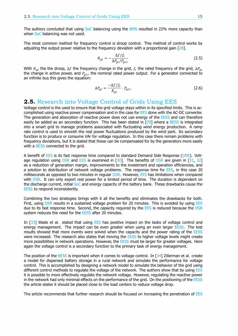
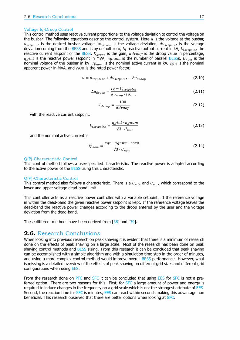
The most common method for frequency control is droop control. This method of control works byadjusting the output power relative to the frequency deviation with a proportional gain [28].
𝑅 = − Δ𝑓/𝑓Δ𝑃 /𝑃 ,
(2.5)
With 𝑅 the the droop, Δ𝑓 the frequency change in the grid, 𝑓 the rated frequency of the grid, Δ𝑃the change in active power, and 𝑃 , the nominal rated power output. For a generator connected toan infinite bus this gives the equation:
Δ𝑃 = −Δ𝑓/𝑓𝑅 ⋅ 𝑃 , (2.6)
2.5. Research into Voltage Control of Grids Using EESVoltage control is the used to ensure that the grid voltage stays within in its specified limits. This is ac-complished using reactive power compensation and in the case for EES done with the AC-DC converter.The generation and absorption of reactive power does not use energy of the EESS and can thereforeeasily be added as an secondary function. This has been stated in [29] where a BESS is integratedinto a smart grid to manage problems associated with fluctuating wind energy production. A ramprate control is used to smooth the real power fluctuations produced by the wind park. Its secondaryfunction is to produce or consume VAr for voltage regulation. In this case there remain problems withfrequency deviations, but it is stated that these can be compensated for by the generators more easilywith a BESS connected to the grid.
A benefit of EES is its fast response time compared to standard Demand Side Response (DSR). Volt-age regulation using DSR and EES is examined in [30]. The benefits of DSR are given in [31, 32]as a reduction of generation margin, improvements to the investment and operation efficiencies, anda solution to distribution of network voltage problems. The response time for EES, in this case 20milliseconds as opposed to two minutes in regular DSR. However, EES has limitations when comparedwith DSR. It can only export real power for a limited period of time. The duration is dependent onthe discharge current, initial SoC and energy capacity of the battery bank. These drawbacks cause theEESS to respond inconsistently.
Combining the two strategies brings with it all the benefits and eliminates the drawbacks for both.First, using DSR results in a sustained voltage problem for 20 minutes. This is avoided by using EESdue to its fast response time. Second, the capacity required by the EES is reduced because the DSRsystem reduces the need for the EESS after 20 minutes.
In [33] Wade et al. stated that using EES has positive impact on the tasks of voltage control andenergy management. The impact can be even greater when using an even larger EESS. The testresults showed that more events were solved when the capacity and the power rating of the EESSwere increased. The research also states that moving the EESS to higher voltage levels might createmore possibilities in network operations. However, the EESS must be larger for greater voltages. Hereagain the voltage control is a secondary function to the primary task of energy management.
The position of the BESS is important when it comes to voltage control. In [34] Zillerman et al. createa model for dispersed battery storage in a rural network and simulate the performance for voltagecontrol. This is accomplished by designing a network model to simulate the behavior of the grid usingdifferent control methods to regulate the voltage of the network. The authors show that by using EESit is possible to more effectively regulate the network voltage. However, regulating the reactive powerin the network had only minimal effects on the performance of the grid. On the positioning of the EESSthe article states it should be placed close to the load centers to reduce voltage drop.
The article recommends that further research should be focused on increasing the penetration of EES

16 2. Research
for improved voltage control. This however might increase the risk of over voltage due to reversecurrent flow in the network. Also, an analytical solution for placing the storage units would allow formore efficient EES. Finally, the authors suggest using a network with higher customer density to testif these results hold or if different control strategies are required.
In [35] Tonkosiki and Lopes’ article calculations with regards to voltage regulation using reactive powercompensation are performed. A simple gird consisting of five buses with high PV generations is used tocalculate the effects. For low voltage it was shown that limiting the over voltage was easier using activepower. This is due to the large R/XL ratio common in low voltage grids. Reactive power compensationis more effective in Medium Voltage (MV) networks where the R/XL ratio is lower.
Similar results were found in [36] where reactive power compensation was used on a low voltagenetwork with high PV penetration.
New research is still being done in the field of voltage control using EES. In paper [37] the authorsdescribe a new control method for minimizing transformer peak-loading using EES. The controller cal-culates the optimal charge and discharge pasterns for a 24-hour receding horizon, based on previousdata, measurements, and the SoC. This controller charging path optimizing control is able to reducepeak loading of the transformer up to 17.9%. More robust control can be achieved by improving pre-diction accuracy. However, it was proven that the algorithm is effective even when utilizing a simpleprediction technique.
There are several control methods to regulate voltage using reactive power. These various meth-ods are listed below, with a short explanation of their working principals. The voltage at a bus barcan be controlled, as described in [38], by supplying and absorbing reactive power. Using a powerelectronic converter the BESS can supply and absorb reactive power from the grid to control the voltageat the bus bar where the system is installed. This method of voltage control has not been successfulfor Low Voltage (LV) girds because of the low 𝑅/𝑋 ratio. However, in MV grids the 𝑅/𝑋 ratio of thegrid is higher so it can be expected that the effect will be greater.
Constant Voltage ControlThis is a local controller where the reactive power of the BESS is controlled to achieve a specified localvoltage at its terminal. The active power is kept constant. The reactive power is increased or decreaseduntil the specified voltage is reached or the reactive power limit of the BESS is reached.
Voltage Q-Droop ControlDroop control corresponds to using a proportional controller to control the voltage level. The amountof reactive power is calculated in proportion to the deviation from the voltage. This controller can beused when multiple BESSs are close together.
The equations below explain the working of the droop control. Here 𝑢 is the voltage at the bus-bar, 𝑢 is the desired voltage level, Δ𝑢 is the voltage deviation, 𝑄 is the reactive poweroutput of the BESS, 𝑄 is the specified dispatch reactive power, 𝑄 is the additional reactivepower for 1% voltage deviation, 𝑆 is the nominal apparent power, and 𝑑𝑑𝑟𝑜𝑜𝑝 is the droop valuespecified in percentage.
𝑢 = 𝑢 − Δ𝑢 (2.7)
Δ𝑢 =𝑄 − 𝑄𝑄 (2.8)
𝑄 = 𝑆 ⋅ 100𝑑𝑑𝑟𝑜𝑜𝑝 (2.9)
2.6. Research Conclusions 17
Voltage Iq-Droop ControlThis control method uses reactive current proportional to the voltage deviation to control the voltage onthe busbar. The following equations describe the control system. Here 𝑢 is the voltage at the busbar,𝑢 is the desired busbar voltage, Δ𝑢 is the voltage deviation, 𝑑𝑢 is the voltagedeviation coming from the BESS and is by default zero, 𝐼𝑞 reactive output current in kA, 𝐼𝑞 thereactive current setpoint of the BESS, 𝐾 is the gain, 𝑑𝑑𝑟𝑜𝑜𝑝 is the droop value in percentage,𝑞𝑔𝑖𝑛𝑖 is the reactive power setpoint in MVA, 𝑛𝑔𝑛𝑢𝑚 is the number of parallel BESSs, 𝑈 is thenominal voltage of the busbar in kV, 𝐼𝑝 is the nominal active current in kA, 𝑠𝑔𝑛 is the nominalapparent power in MVA, and 𝑐𝑜𝑠𝑛 is the rated power factor.
𝑢 = 𝑢 + 𝑑𝑢 − Δ𝑢 (2.10)
Δ𝑢 =𝐼𝑞 − 𝐼𝑞𝐾 ⋅ 𝐼𝑝 (2.11)
𝐾 = 100𝑑𝑑𝑟𝑜𝑜𝑝 (2.12)
with the reactive current setpoint:
𝐼𝑞 = 𝑞𝑔𝑖𝑛𝑖 ⋅ 𝑛𝑔𝑛𝑢𝑚√3 ⋅ 𝑈
(2.13)
and the nominal active current is:
𝐼𝑝 = 𝑠𝑔𝑛 ⋅ 𝑛𝑔𝑛𝑢𝑚 ⋅ 𝑐𝑜𝑠𝑛√3 ⋅ 𝑈
(2.14)
Q(P)-Characteristic ControlThis control method follows a user-specified characteristic. The reactive power is adapted accordingto the active power of the BESS using this characteristic.
Q(V)-Characteristic ControlThis control method also follows a characteristic. There is a 𝑈 and 𝑈 which correspond to thelower and upper voltage dead-band limit.
This controller acts as a reactive power controller with a variable setpoint. If the reference voltagein within the dead-band the given reactive power setpoint is kept. If the reference voltage leaves thedead-band the reactive power changes according to the droop entered by the user and the voltagedeviation from the dead-band.
These different methods have been derived from [38] and [39].
2.6. Research ConclusionsWhen looking into previous research on peak shaving it is evident that there is a minimum of researchdone on the effects of peak shaving on a large scale. Most of the research has been done on peakshaving control methods and BESS sizing. From this research it can be concluded that peak shavingcan be accomplished with a simple algorithm and with a simulation time step in the order of minutes,and using a more complex control method would improve overall BESS performance. However, whatis missing is a detailed overview of the effects of peak shaving on different grid sizes and different gridconfigurations when using EES.
From the research done on PFC and SFC it can be concluded that using EES for SFC is not a pre-ferred option. There are two reasons for this. First, for SFC a large amount of power and energy isrequired to induce changes in the frequency on a grid scale which is not the strongest attribute of EES.Second, the reaction time for SFC is minutes, EES can react within seconds making this advantage nonbeneficial. This research observed that there are better options when looking at SFC.

18 2. Research
A PFC EES is a valid option when reaction times have to be fast and power is only required for shortperiods of time. However, due to the fact that these effects take place on a millisecond to a secondtime scale which does not coincide with the minute time scale of peak shaving, PFC is dropped in favorof peak shaving.
Based on the research conducted on voltage control in can be concluded that it is beneficial to use EESfor voltage regulation as it has quick response times for load-flowing and peak-shaving. The researchperformed on reactive power compensation showed minimal improvements when using EES. It is rec-ommend to move the EESS from LV networks, where tests were conducted, to MV networks wherethe R/XL ratio is lower in order for reactive power compensation to have a greater effect. However,this results in the need for a larger EESS to handle the increased power consumption of a MV network.Implementing EESs in conjunction with other control methods such as DSR helps reduce the drawbacksof both systems and can greatly improve grid performance.
The information and results obtained from the articles cited above make it possible to determine whereadditional research is required to further study the effects and benefits of EES. The following sectioncontains an outline of these additional research objective requirements.
2.7. Research ObjectiveMuch research has been done in the area of EES. However, when examining the literature it becomesobvious that there is a research gap in the area of effects of peak shaving on MV networks using EES.This thesis will attempt to close this gap by conducting a research on:
• power supply capacity increase,
• congestion relief,
• transmission upgrade deferral, and
• distribution upgrade deferral
in MV networks using EES in the form of a BESS for peak shaving.
The focus of the research will be on the benefits and the drawbacks to the network when apply-ing these control systems to the grid. In this process the thesis will provide answers to the followingquestions.
• Is it possible to reduce the load peaks using EES?
• Does reducing the load peaks reduce congestion within the grid?
• Does reducing the load peaks reduce energy losses?
• What will be the impact in the future of an increase in sustainable energy mix and increasingdemand stimulated by Electric Vehicle?
• Will a simple peak shaving algorithm still be sufficient in the future?
• What will the effect of these future scenarios be on the size requirements of EES?
Each of these questions will be examined by simulating a MV network using different scenarios. Eachof these scenarios is detailed in Chapter 3. The network models used as the basis for this research willbe created, built, and simulated using the PowerFactory software tool provided by DigSilent.
2.8. Rules and Regulations with Regards to EES Grid IntegrationFor integrating EES into the grid there are rules and regulations in the form of IEC standards. However,because EES is a relatively new technology, the list of standards is still a work in progress and shouldtherefore be considered incomplete. For this reason the GRIDSTORE project required an overview ofexisting standards that play a role in EES grid connection. The thesis research is based on the list ofrules and regulations that are provided in Appendix A.
3Models and Simulation Scenarios
In this chapter the reference gird is described to which the peak shaving method will be tested. Thereference grid is then used to construct the grid model and the BESS model. These two models arethen discussed and the six simulation scenarios for the real world case are described.
3.1. Reference CaseAs a reference case an example network from PowerFactory is used. This nine node network wasintroduced in the book Power System Control and Stability by P.M. Anderson and A. A. Fouad [40].This test case is chosen because of its simplicity with only nine nodes. The details of this feeder aregiven in Appendix B. Bus 5 is where Load A is connected and where the BESS is added so it is as closeas possible to the load. The nominal voltage of this test network is 230 kV. The connection betweenLine 3-5 and Bus 5 is closed to create a radial configured feeder to Load A.
3.2. Real World CaseFor the second case simulations an existing MV power grid was modeled in Vision and then convertedusing PowerFactory so dynamic simulations could be run on the different scenarios. The power gridis based on the actual distribution grid on the island of Goeree-Overflakkee in the province of South-Holland, The Netherlands. Figure 3.1 shows the geographic location of this island. The Goeree-Overflakkee distribution system has two major substations located in Stellendam and Middelharnis.Both of these substations are responsible for distributing energy to the consumers. In order to achievepeak shaving the BESSs are to be integrated into the Stellendam distribution system. Both substationshave high renewable energy penetration in the form of wind and solar energy production.
3.2.1. Goeree-OverflakeeThe municipality of Goeree-Overflakee has a total area of 261 km2 and a population of approximately48,000 spread over 19 towns and villages. Given the ratio of population to area, this is consideredlow density in The Netherlands. Because of its low population density and proximity to the sea, it is apopular venue for holidays especially during the summer months [41].
There are a number of natural energy sources present on Goeree-Overflakee. The area benefits from ahigh amount of sun hours per year and relatively high wind speeds. Goeree-Overflakee has the ambi-tion of realizing an energy neutral position by the year 2030. This implies that energy production fromrenewable energy sources will be required to meet the total energy consumption of the municipality.
The current annual energy consumption is estimated to be 992 GWh, but is expected to decline to553 GWh as a result of planned energy savings. Currently 22% of the total energy consumption isproduced by wind turbines.
19

20 3. Models and Simulation Scenarios
Figure 3.1: Goeree-Overflakee
3.2.2. The Distribution SystemThe distribution system on Goeree-Overflakee is fed by a 52.5 kV underground cable coming in fromthe mainland. The underground cable is connected to twelve 2 MVA wind turbines operating at a volt-age of 23 kV and to the substation of Middelharnis. Substation Stellendam is connected to substationMiddelharnis via two 52.5 kV underground cables.
For the simulations the 13 kV distribution system on Goeree-Overflakee is used. This distributionsystem has been chosen because it is already integrated in place and integrated over the island andcan be used to connect even larger loads if desired. In addition, the topology of the system greatlyresembles distribution systems in the rest of the Netherlands. This ensures that the simulations canbe related to other distribution networks within the Netherlands.
The 13 kV distribution systems are connected to two main substations: Middelharnis and Stellendam.Because these two distribution networks are similar for the simulations, the choice has been made touse the 13 kV distribution system of Stellendam, Figure 3.2. A model of this distribution system hasbeen created in PowerFactory using the original Vision files as a point of departure. Modeling using Vi-sion produces static models while using PowerFactory allows for dynamic modeling. The PowerFactoryand Vision single line diagram models can be found in Appendix C. The external grid connection to thisdistribution system is modeled as an infinity strong voltage source with a corresponding R/X ratio of0.35 and a short-circuit power of 320 MVA.
3.3. BESS ModelIn Chapter 4 simulations are run in different scenarios to determine the effects of a BESS on theStellendam distribution system. In order to run these simulations, a model of the BESS is needed. Thismodel is created using DigSILENT Programming Language (DPL) and the battery storage element fromPowerFactory. The battery storage element models a static generator with additional parameters toenable it to resemble a BESS. The model includes a DC-AC/AC-DC converter to allow it to be connecteddirectly to the grid. However, the model does not include a SoC control system. A SoC control systemis needed in order to keep track of the energy available in the BESS. If the SoC reaches its full or emptyvalue, the BESS should stop charging or discharging. For this reason it is important the SoC controlsystem is created.

3.3. BESS Model 21
Figure 3.2: Stellendam Distribution System
The model has a control program for calculating output power and keeping track of the SoC usingDPL. In order to calculate the output power an input reference is required. This input reference ispower. From here the output power can be calculated for different scenarios. How the input referenceis measured or calculated can be altered for each use of the BESS. For example, with peak shavingthe input power is calculated from the cables connected to the busbar to which the BESS is connected.The output is always power-delivered to the busbar to which the BESS is connected. The BESS can ofcourse deliver (+) or consume (-) power.
There are four cases that have to be handled:
• regular discharge,
• regular charge,
• empty discharge, and
• full charge.
The SoC must remain between 40% and 60% according to the Network Code on EESS reserves. Soboth regular charge and discharge occurs when the SoC value is safely between these values. Safelymeaning there there is no possibility of the SoC exceeding the 40% value in case of discharging andthe 60% value in case of charging. In these cases the SoC is calculated using the following equation:
𝑆𝑜𝐶 = 𝑆𝑜𝐶 ⋅ 𝐶 − 𝐸𝐶 (3.1)
where 𝑆𝑜𝐶 is the new SoC value after running the load flow calculation, 𝑆𝑜𝐶 is the old SoCbefore running the load flow calculation, 𝐶 is the BESS capacity in kWh, and 𝐸 is the energyproduced (+) or consumed (-) by the BESS.
For the empty discharge and full charge cases a different calculation is required. As it is not pos-sible to discharge more than 40% of the BESS or charge more than 60% of the BESS it is necessarythat when the next time step calculation will exceed these values the remaining energy is calculatedrather than the new SoC, as is done in the other cases. Therefor, the old SoC is compared to the SoClimit in order to calculate the remaining energy as is shown in the following equation:
𝐸 = (𝑆𝑜𝐶 − 𝑆𝑜𝐶 ) ⋅ 𝐶 (3.2)Here 𝑆𝑜𝐶 is the upper or lower SoC limit of the BESS. The remaining energy is 𝐸 and thisis what is delivered or consumed by the grid. The delivered energy can be positive in case of energydelivered or negative in the case of consumed energy.

22 3. Models and Simulation Scenarios
Table 3.1: Normal consumer size loads
Load Size Load Size
PZ1 0.974 MVA ZS3 0.31 MVAPZ2 0.387 MVA ZS4 249 kVAPZ3 0.532 MVA ZS5 120 kVAPZ4 0.184 MVA ZS6 241 kVABG1 553 kVA ZS7 321 kVABG2 193 kVA ZS8 218 kVABG3 34 kVA ZS9 355 kVAZS1 756 kVA ZS10 590 kVAZS2 392 kVA ZS11 1170 kVA
3.4. Simulation ScenariosThe current consumer size loads for the Stellendam distribution grid are given in Table 3.1. Thesevalues are taken directly from the Vision models and represent the actual measured average loads inthis distribution system.
It is expected that the BESS can reduce strains on the grid in the form of congestion relief and atthe same time help reduce the losses in transmission cables by reducing the load. However, the Stel-lendam distribution system is overly robust, greatly over-dimensioned to cope with future growth inboth renewable energy sources and consumers. For the effects to be clear, the current scenario willbe compared to future scenarios where the grid will have 10 - 100% more consumers. The scenariosfor analysis are:
• at current consumer size,
• a 20% consumer size increase,
• a 50% consumer size increase, and
• a 100% consumer size increase.
Two additional scenarios have been added to each scenario to examine the effects of increased usageof EVs and increased implementation of Renewable Energy (RE). The additional scenarios are thereforedefined as:
• increase of RE in the form of solar panels, and
• increase of load in the form of EV.
These scenarios are applied to three different locations of the Stellendam distribution system; feeder204, feeder 103, and feeder 111. Feeder 103 has a radial configuration and feeder 204 a meshedconfiguration. Using these two different locations, the effects on a radial distributed feeder and ameshed feeder can be analyzed. Feeder 111 will be analyzed using these different scenarios becausethis location has the highest load on its connection cables of the whole distribution system.
The current consumer loads are based on actual measurements within the feeders. The growth ofthe loads is the same for all different consumer type loads. For a growth of 20% there would be 20%more households, normal commerce, weekday commerce and weekend operation. The same appliesto the 50% and 100% increases. The different consumer types are explained in the next section.

3.5. Load Profiles 23
3.5. Load ProfilesIn order to create a dynamic simulation load profiles are needed with a variation in loads throughoutthe day. Six different profiles are needed for the simulation: four different load profiles for regularconsumers, a generation profile for the PV, and an extra load profile for the energy consumption of anEV. The load profiles exist of 96 fifteen minute time steps.
3.5.1. Regular Consumer Load ProfilesTo simulate load changes during, the day load profiles are used on the connected loads. The fourdifferent load profiles used are:
• household,
• normal commerce,
• weekday commerce, and
• weekend operation.
The load profiles have been chosen per load based on the location of the substation. A winter weekdayhas been chosen as it is expected that this is when most electricity is used. Actual load profile data wasprovided by Joulz. However, due to privacy constraints it is not possible use this actual data. In orderto make accurate simulations different standard load profiles were used. These load profiles comewith the PowerFactory software and were compared to the real world load profiles in order to find themost corresponding profile. The load profiles that were chosen and shown in Figure 3.3 resemble thedifferent real world load profiles the most.
0 6 12 18 240
0.5
1
Time [h]
Load
ing[%
]
Household Load Profile
(a) Household
0 6 12 18 240
0.5
1
Time [h]
Load
ing[%
]
Normal Commerce Load Profile
(b) Normal Commerce
0 6 12 18 240
0.5
1
Time [h]
Load
ing[%
]
Weekday Commerce Load Profile
(c) Weekday Commerce
0 6 12 18 240
0.5
1
Time [h]
Load
ing[%
]
Weekend Operation Load Profile
(d) Weekend Operation
Figure 3.3: Load Profiles

24 3. Models and Simulation Scenarios
3.5.2. EV Consumption ProfileEVs are generally used during the day and charged at home at night. For these reasons a load profilewith the bulk of charging occurring at night is choses to represent the EV load profile. The load profileshown in Figure 3.4 is used with the bulk of vehicles charging between 0 and 8 hours. An EV is said tohave a load of 3.7 kW according to [42] when charged at home. This load is scaled to the amount ofEV assumed to be in the neighborhood.
0 2 4 6 8 10 12 14 16 18 20 22 240
0.2
0.4
0.6
0.8
1
Time [h]
Load
ing[%
]
Electric Vehicle Load
Figure 3.4: EV Load Profile
3.5.3. PV ProfileIt is anticipated that in the period under examination more households will have PV panels to producesolar energy for their own use. Unused energy production is returned to the grid. To simulate thisgrowth in energy production, it is assumed each household has 10 solar panels with the solar panel pa-rameters given in Table 3.2. The power output for one household during the day is shown in Figure 3.5.This profile is based on the solar calculation using the parameters given in Table 3.3.
0 2 4 6 8 10 12 14 16 18 20 22 240
0.5
1
Time [h]
Power
[kW]
PV Output One Household
Figure 3.5: PV Output Profile for one Household

3.5. Load Profiles 25
Table 3.2: PV Module Parameters
Parameter Value
Type BP SX 110 S 12 VMaterial Polycrystalline SiliconPeak Power 110 WRated Voltage 16.4 VRated Current 6.7 AOpen Circuit Voltage 20.6 VShort Circuit Current 7.38 A
Table 3.3: Solar Calculation Parameters
Parameter Value
Specified Components Global and DiffuseGlobal Irradiance Data Adnot-Bourges et.al. ModelDiffuse Irradiance Data Louche et.al. ModelAmbient Temperature 8 ∘CShading Factor Direct 0Shading Factor Diffuse 0Ground Albedo 0.31Latitude 51° 49 6 NLongitude 3° 54 8 ETilt Angle 30°Efficiency Factor 95%

4Simulations and Results
In this chapter the scenarios referred to and described in the previous chapter are simulated and theresults of these simulations analyzed. As previously discussed in Chapter 2, peak shaving can havemultiple benefits when applied to a MV network. Therefore, the simulations are run using peak shavingfor each of the scenarios presented in Chapter 3.
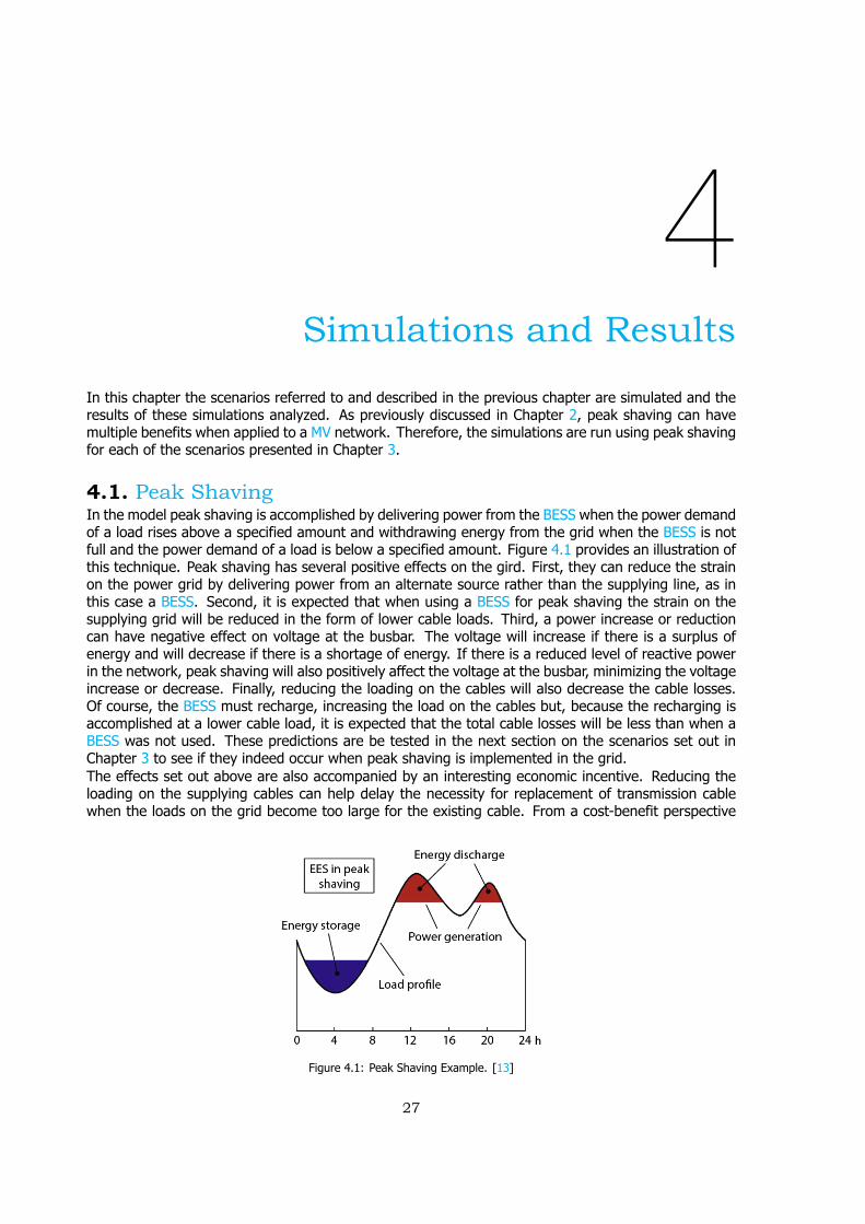
4.1. Peak ShavingIn the model peak shaving is accomplished by delivering power from the BESS when the power demandof a load rises above a specified amount and withdrawing energy from the grid when the BESS is notfull and the power demand of a load is below a specified amount. Figure 4.1 provides an illustration ofthis technique. Peak shaving has several positive effects on the gird. First, they can reduce the strainon the power grid by delivering power from an alternate source rather than the supplying line, as inthis case a BESS. Second, it is expected that when using a BESS for peak shaving the strain on thesupplying grid will be reduced in the form of lower cable loads. Third, a power increase or reductioncan have negative effect on voltage at the busbar. The voltage will increase if there is a surplus ofenergy and will decrease if there is a shortage of energy. If there is a reduced level of reactive powerin the network, peak shaving will also positively affect the voltage at the busbar, minimizing the voltageincrease or decrease. Finally, reducing the loading on the cables will also decrease the cable losses.Of course, the BESS must recharge, increasing the load on the cables but, because the recharging isaccomplished at a lower cable load, it is expected that the total cable losses will be less than when aBESS was not used. These predictions are be tested in the next section on the scenarios set out inChapter 3 to see if they indeed occur when peak shaving is implemented in the grid.The effects set out above are also accompanied by an interesting economic incentive. Reducing theloading on the supplying cables can help delay the necessity for replacement of transmission cablewhen the loads on the grid become too large for the existing cable. From a cost-benefit perspective
Figure 4.1: Peak Shaving Example. [13]
27

28 4. Simulations and Results
installing a BESS may be a more economical solution then installing a brand new cable. Further, if re-ducing the load on the transmission cables reduces the losses in the cable, then this will cut productioncosts which are beneficial for both consumers and producers.
An additional benefit of this peak shaving analysis is that it will also shed light on the amount ofreactive power in the grid. If voltage on the busbar continues to drop during peak operation whilepeak shaving is active, this may indicate that there is an abundance of reactive power in the grid, andreactive power compensation for voltage control may need to be analyzed further in the extra scenarios.
In order to model peak shaving within PowerFactory for application to various scenarios, a DPL controlprogram has been written to provide for the supply to and demand for energy from the grid. The DPLcontrol program code can be found in Appendix D. The control program works with a power input anda power output as discussed in Chapter 3. In the model from the point where the SoC reaches a levelgreater than 40%, the BESS begins to supply power. The 40% is referred to as the “lower SoC limit”.The limit chosen is a percentage of the max load of the cable for which the load is to be reduced. Thisparameter is defined as the Maximum Cable Load (MCL). The MCL is calculated as a percentage of themaximum current allowed through the cable.
𝐼 = √3 ⋅ 𝐼 , ⋅ 𝑀𝐶𝐿% (4.1)
With 𝐼 the maximum cable load current defined by the user, 𝐼 , the maximum current al-lowed by the specifications of the cable, and 𝑀𝐶𝐿% the percentage of the maximum current for whenthe user wants to start peak shaving.
A similar equation is used to define the cable load at which the BESS is allowed to recharge. Forthe BESS to recharge, the supplying cable load has to be lower than the Maximum Recharge CableLoad (MRCL). In the model the BESS recharges to a SoC of 50%, called the “default SoC”, as long asthe cable load does not rise above maximum recharge cable load.
𝐼 = √3 ⋅ 𝐼 , ⋅ 𝑀𝑅𝐶𝐿% (4.2)
Here the 𝐼 is the maximum cable load current defined by the user, and 𝑀𝑅𝐶𝐿% the percentage ofthe maximum cable current at which the BESS has to stop charging.
The next step is to calculate the amount of current the BESS has to deliver to the network in order tostay below this MCL. This current is calculated with the following equation:
𝐼 = 𝑃 − 𝑃𝑈 − 𝐼 (4.3)
Where 𝐼 is the current the BESS has to supply, 𝑃 is the power requested from the loadat the busbar, 𝑃 is the incoming power to the busbar, and 𝑈 is the current busbar voltage.
It is also necessary to know the maximum current the BESS can request from the grid without surpass-ing the MRCL. This is done using the following equation:
𝐼 = 𝑃 + 𝑃 − 𝑃𝑈 − 𝐼 (4.4)
Here 𝐼 is negative as the BESS is recharging. 𝐼 is swapped for 𝐼 and the last powerconsumption state of BESS is added as 𝑃 in order to determine the new state. If this parameteris not added the MRCL will be exceeded during the following load flow calculation. This will causethe BESS to stop charging. The load will then drop below MRCL and start charging repeating theprocess. This process causes the BESS state to fluctuate between charging and discharging. Addingthis parameter removes this fluctuation.

4.2. Reference Case Simulation 29
Now the charge and discharge currents are known it is possible to define three BESS states:
• charge,
• discharge, and
• idle.
The discharge state is entered if 𝐼 current larger than 0. This entails that the MCL has beenexceeded and additional power is needed from the BESS.
The charge state is reached if 𝐼 and 𝐼 are both lower than 0. This means that thecable load is not over the MCL and there is room to increase the load the MRCL to charge the BESS.
The idle state is if none of the above states are reached, so if 𝐼 is lower or equal to 0,but 𝐼 higher or equal to 0. Or if the SoC has reached one of its limits.
The penultimate step is to calculate the actual power power consumed (-) or supplied (+) by theBESS depending on the state.
𝑃 = 𝑈 ⋅ (𝐼 or 𝐼 ) (4.5)
The last step is to calculate the 𝐸 parameter in order to find the new SoC value. This is done withthe following equation:
𝐸 = 𝑃4 (4.6)
The constant is determined due to a simulation time step of 15 minutes. There are four time steps inevery our so the power has to be divided by 4 to arrive at the used energy. These steps are genericfor each of the scenarios.
4.2. Reference Case SimulationThe first case that is simulated is the nine node network given in [40]. As noted above the details ofthis network can be found in Appendix B. For the simulation only bus 1, 4 and 5 are used to createa radial configured feeder. Line 5-7 and 4-6 are disconnected from this feeder and generator G1 isreplaced with an external grid. This configuration is provided to create a situation that resembles thereal world case in the next simulation more which is required to objectively compare the two. The loadis 125 MW with a power factor of 0.928 and given the profile of a household. Peak shaving is set to limitthe cable load to 25%. The maximum cable load to which the BESS is allowed to recharge is set to 20%.
The BESS has a power limit of 20 MW. This limit is rather large, but because the network has alarge load this is a necessity in order to test the peak shaving algorithm. For the same reason the sizeof the BESS is not taken into account.
Figure 4.2 shows that the BESS commences supplying power between six and seven pm. When com-paring this with the cable load in Figure 4.3 it can be observed that the cable load passed the 25%mark at this time causing the BESS to start supplying power in order to limit the cable load until thecable load drops back below 25%. It can also be observed that when the cable load drops below 20%the BESS starts to recharge with the available power until the SoC reaches 50%. This activity is clearlyvisible in the negative portion of the graph in Figure 4.2. Figure 4.4 shows that the reduction of thecable load has a positive effect on the cable losses. Recharging the BESS increases the cable load andtherefor also the cable losses.
It is obvious from these results that the peak shaving algorithm is functioning as is intended. It isnow possible to continue to the real world case and examine the effects of peak shaving on a realworld network.

30 4. Simulations and Results
0 6 12 18 24−20
−10
0
10
20
Time [h]
Power
[MW]
BESS Power Output
Figure 4.2: BESS Power Output
0 6 12 18 24
10
20
30
Time [h]
Load
ing[%
]
Cable Loading
Loading w/o BESSLoading w/ BESS
Figure 4.3: Cable Loading
0 6 12 18 240
0.5
1
1.5
Time [h]
Losses
[MW]
Cable Losses
Losses w/o BESSLosses w/ BESS
Figure 4.4: Cable Losses

4.3. Real World Case 31
Table 4.1: Simulation Parameters
Parameter Value Description
BESS Size 15 kWh Energy capacity of all the BESSsMaximum BESS Output Power 3 kW Maximum output power of the BESSsTime Step Size 15 min. Time step size for each following load flow calculationMCL feeder 204 18% Value above which the BESS will start delivering powerMCL feeder 103 9% Value above which the BESS will start delivering powerMCL feeder 111 55% Value above which the BESS will start delivering powerMRCL feeder 204 16% Value above which the BESS will stop chargingMRCL feeder 103 8% Value above which the BESS will stop chargingMRCL feeder 111 50% Value above which the BESS will stop charging
4.3. Real World CaseThis section provides the results of the different scenarios set out in Chapter 3. They are:
• at current consumer size,
• a 20% consumer size increase,
• a 50% consumer size increase, and
• a 100% consumer size increase.
With two additional scenarios:
• an increase of RE in the form of solar panels, and
• an increase of load in the form of EV.
These scenarios are analyzed on three different feeders. The BESSs are connected to busbars in thefeeders. These feeders are: feeder 204, Port Zelande; feeder 103, Bed. Geb.; and feeder 111, ZendStation.Before running the different scenarios through the simulation model, several parameters which remainconstant during all the simulations require definition. Their value and the description of these param-eters are provided in Table 4.1. This table shows the MCL and MRCL for the three feeders. The timestep for the simulation is set to 15 minutes. This setting implies that every 15 minutes a new loadflow will be run to determine the BESS power output/input and the new SoC. The BESS size is givenas 15kWh 5 times the maximum power output of the BESS. The results of the various simulations areprovided in this section.
4.3.1. Scenario Current Consumer SizeFirst the BESS energy production and consumption shown in Figure 4.6 is examined. It can be observedthat there is no power production or consumption by the BESS. This can be explained by referring toFigure 4.7. Here it can be seen that none of the cables reach the critical load required for the BESS tobegin delivering power. For this scenario the results are that there is no change in busbar voltage orloss reduction in the cables. This is visible in Figure 4.7 and Figure 4.8.

32 4. Simulations and Results
0 6 12 18 240
1
2
Time [h]
Power
[MW]
Load Profiles at Normal Load
Port ZelandeBed. Geb.Zend Station
Figure 4.5: Load Profiles at Current Load
0 6 12 18 24−1
−0.5
0
0.5
1
Time [h]
Power
[MW]
BESS Power Output Normal Load
BESS Port ZelandeBESS Bed. Geb.BESS Zend Station
Figure 4.6: BESS Power Output at Current Consumer Load
0 6 12 18 240
20
40
Time [h]
Load
ing[%
]
Cable Loading Normal Load
Cable Port ZelandeCable Bed. Geb.Cable Zend Station
Figure 4.7: Cable Loading at Current Consumer Load

4.3. Real World Case 33
Table 4.2: Cable Energy Losses Comparison at 120%
Cable w\o BESS w\ BESS Difference
Cable Port Zelande 167.26 kWh 162.34 kWh 4.92 kWhCable Bed. Geb. 11.23 kWh 11.24 kWh -0.01 kWhCable Zend Station 1719.7 kWh 1721.6 kWh -1.9 kWh
4.3.2. Scenario 120% Consumer SizeIn this scenario the consumer loads are increased by 20%. Reviewing the energy production andconsumption of the BESS in Figure 4.10, it is observed that there is indeed energy production andconsumption by the BESS on all three feeders. This implies that the cable loads have reached theirMCL. Therefore it is possible to move to the next step and compare the cable load with and withoutthe BESS. These results are presented in Figure 4.11, Figure 4.12, and Figure 4.13.
In these figures the loading of the cables of which the load is being limited are shown. From thesefigures it is clear (dashed line) that the cable load is reduced to the MCL when the cable load surpassesthe MCL value set in Table 4.1. It is also clear that the cable load increases when the BESS is charg-ing. This raises the question: does the reduction of losses during peak shaving out weighs the lossesthat are increased while recharging the BESS. Therefor, the cable losses with and without BESS arecompared in Figure 4.14, Figure 4.15, and Figure 4.16.
The total losses are expected to be reduced because the BESS is charged at a lower cable load. Thiscan be verified by integrating the difference between the losses with BESS and the losses without BESS.Shown in the following equation:
𝐸 , = ∫ 𝑃 , (𝑡)𝑑𝑡 − ∫ 𝑃 , (𝑡)𝑑𝑡 (4.7)
Where 𝐸 , is the saved or lost energy, 𝑃 (𝑡) the graph of the cable losses with BESS and𝑃 , (𝑡) the graph of the cable losses without BESS.
These results are provided in Table 4.2. The results deviate from those anticipated as they show asmall increase in cable losses for feeders 103 and 111. This is due to the numerical integration methodused for calculating the energy loss. This should disappear when the differences become more obviousin the other scenarios.
Next the busbar voltage is examined for the three different locations to determine if the busbar voltagedrop can be minimized using peak shaving only. Examining Figure 4.17, Figure 4.18, and Figure 4.19,a slight improvement is observed. The minimum busbar voltage values are shown in Table 4.3 wherethe slight improvement can also be seen.
Table 4.3: Minimum values of busbar voltages at 120%
Busbar w\o BESS w\ BESS
Port Zelande 0.9685 pu 0.9697 puBed. Geb. 0.9930 pu 0.9932 puZend Station 0.9560 pu 0.9573 pu

34 4. Simulations and Results
0 6 12 18 240.96
0.98
1
1.02
Time [h]
Volta
ge[pu]
Busbar Voltages Normal Load
Port ZelandeBed. Geb.Zend Station
Figure 4.8: Busbar Voltages at Current Consumer Load
0 6 12 18 240
1
2
3
Time [h]
Power
[MW]
Load Profiles at 120% Load
Port ZelandeBed. Geb.Zend Station
Figure 4.9: Load Profiles at 120% Load
0 6 12 18 24−0.3
−0.2
−0.1
0
0.1
Time [h]
Power
[MW]
BESS Power Output 120% Load
BESS Port ZelandeBESS Bed. Geb.BESS Zend Station
Figure 4.10: BESS Power Output 120% Load

4.3. Real World Case 35
0 6 12 18 240
10
20
Time [h]
Load
ing[%
]Port Zelande Cable 1 Loading at 120% Load
Loading w/o BESSLoading w/ BESS
Figure 4.11: Cable Loading at Port Zelande
0 6 12 18 24
2
4
6
8
10
Time [h]
Load
ing[%
]
Bed. Geb. Cable Loading at 120% Load
Loading w/o BESSLoading w/ BESS
Figure 4.12: Cable Loading at Bed. Geb.
0 6 12 18 24
20
40
60
Time [h]
Load
ing[%
]
Zend Station Cable Loading at 120% Load
Loading w/o BESSLoading w/ BESS
Figure 4.13: Cable Loading at Zend Station

36 4. Simulations and Results
0 6 12 18 240
2
4
6
Time [h]
Power
[kW]
Port Zelande Cable 1 Losses at 120% Load
Losses w/o BESSLosses w/ BESS
Figure 4.14: Cable Losses at Port Zelande
0 6 12 18 240
0.1
0.2
0.3
Time [h]
Power
[kW]
Bed. Geb. Cable Losses at 120% Load
Losses w/o BESSLosses w/ BESS
Figure 4.15: Cable Losses at Bed. Geb.
0 6 12 18 240
10
20
30
40
Time [h]
Power
[kW]
Zend Station Cable Losses at 120% Load
Losses w/o BESSLosses w/ BESS
Figure 4.16: Cable Losses at Zend Station

4.3. Real World Case 37
0 6 12 18 24
0.98
1
Time [h]
Volta
ge[pu]
Voltage Busbar Port Zelande. at 120% Load
Voltage w/o BESSVoltage w/ BESS
Figure 4.17: Busbar voltage Port Zelande
0 6 12 18 24
1
1
1.01
1.01
Time [h]
Volta
ge[pu]
Voltage Busbar Bed. Geb. at 120% Load
Voltage w/o BESSVoltage w/ BESS
Figure 4.18: Busbar Voltage Bed. Geb.
0 6 12 18 24
0.96
0.98
1
Time [h]
Volta
ge[pu]
Voltage Busbar Zend Station. at 120% Load
Voltage w/o BESSVoltage w/ BESS
Figure 4.19: Busbar Voltage Zend Station

38 4. Simulations and Results
Table 4.4: Cable Energy Losses Comparison at 150%
Cable w\o BESS w\ BESS Difference
Cable Port Zelande 256.62 kWh 215.03 kWh 41.59 kWhCable Bed. Geb. 15.97 kWh 15.06 kWh 0.91 kWhCable Zend Station 2774.5 kWh 2700.7 kWh 73.8 kWh
4.3.3. Scenario 150% Consumer SizeIncreasing the consumer load to 150% of their original value makes it immediately obvious in Fig-ure 4.21 that the BESS for feeder 111 runs out of energy around 11 hrs. This is evidenced by thesudden steep drop to zero power output. The other two BESSs have enough energy to cope withthe load increase. However, due to the load increase the load does not drop to levels that allow forcharging the BESS early enough to ensure a full charge at the end of the day for all the BESSs. Thiscan be observed as the BESS is still charging at 24 hrs. The respective SoCs of the differentBESSsare 45.0636% for Port Zelande, 50.00806% for Bed. Geb., and 49.0558% for Zend Station. Froma practical standpoint this does not create a problem as the BESS can also charge in the morning ofthe next day. This can be observed when running the simulation for the next 24 hours. This ‘48 hoursimulation’ is shown in Figure 4.22. The ‘48 hour simulation’ results form the basis for a further analysisof this scenario as it provides a more complete picture of the situation.
Cable loads are reduced for all feeders but, once the BESS at feeder 111 runs out of energy, theload of the cable follows the other graphs path. This is visible in Figure 4.25 as the sharp rise. Energylosses in the cables are reduced during discharging as can be seen in Figure 4.23, Figure 4.27 andFigure 4.25. The cable losses for both situations, with and without BESS, are given in Table 4.4. Itis possible to use compare the losses with and without BESS as we did before by integrating the twographs and subtracting them from each other. Now that the losses are larger, the numerical integrationfunctions more completely, and it is clear that there is a small amount of energy saved when comparedto the simulation without peak shaving.
When examining at the busbar voltages, again a small improvement can be perceived. For the busbarat Zend Station the improvement is clear. The minimal values of the busbar voltages are given inTable 4.5. The minimum voltage of the busbar at Zend Station is taken before the BESS runs out ofenergy.
Table 4.5: Minimum values of busbar voltages at 150%
Busbar w\o BESS w\ BESS
Port Zelande 0.9607 pu 0.9658 puBed. Geb. 0.9902 pu 0.9908 puZend Station 0.9429 pu 0.9544 pu

4.3. Real World Case 39
0 6 12 18 240
1
2
3
Time [h]
Power
[MW]
Load Profiles at 150% Load
Port ZelandeBed. Geb.Zend Station
Figure 4.20: Load Profile at 150% Load
0 6 12 18 24
−1
−0.5
0
0.5
Time [h]
Power
[MW]
BESS Power Output 150% Load
BESS Port ZelandeBESS Bed. Geb.BESS Zend Station
Figure 4.21: BESS Power Output at 150% Load
0 6 12 18 24
−1
0
1
Time [h]
Power
[MW]
BESS Power Output 150% Load 48 hrs
BESS Port ZelandeBESS Bed. Geb.BESS Zend Station
Figure 4.22: BESS Power Output at 150% Load second 24 hrs

40 4. Simulations and Results
0 6 12 18 240
10
20
30
Time [h]
Load
ing[%
]
Port Zelande Cable 1 Loading at 150% Load 48 hrs
Loading w/o BESSLoading w/ BESS
Figure 4.23: Cable Loading at Port Zelande
0 6 12 18 24
5
10
Time [h]
Load
ing[%
]
Bed. Geb. Cable Loading at 150% Load 48 hrs
Loading w/o BESSLoading w/ BESS
Figure 4.24: Cable Loading at Bed. Geb.
0 6 12 18 24
20
40
60
80
Time [h]
Load
ing[%
]
Zend Station Cable Loading at 150% Load 48 hrs
Loading w/o BESSLoading w/ BESS
Figure 4.25: Cable Loading at Zend Station

4.3. Real World Case 41
0 6 12 18 240
2
4
6
8
Time [h]
Power
[kW]
Port Zelande Cable 1 Losses at 150% Load 48 hrs
Losses w/o BESSLosses w/ BESS
Figure 4.26: Cable Losses at Port Zelande
0 6 12 18 240
0.1
0.2
0.3
0.4
Time [h]
Power
[kW]
Bed. Geb. Cable Losses at 150% Load 48 hrs
Losses w/o BESSLosses w/ BESS
Figure 4.27: Cable Losses at Bed. Geb.
0 6 12 18 240
20
40
60
Time [h]
Power
[kW]
Zend Station Cable Losses at 150% Load 48 hrs
Losses w/o BESSLosses w/ BESS
Figure 4.28: Cable Losses at Zend Station

42 4. Simulations and Results
0 6 12 18 240.96
0.98
1
Time [h]
Volta
ge[pu]
Voltage Busbar Port Zelande. at 150% Load 48 hrs
Voltage w/o BESSVoltage w/ BESS
Figure 4.29: Busbar voltage Port Zelande
0 6 12 18 240.99
1
1.01
Time [h]
Volta
ge[pu]
Voltage Busbar Bed. Geb. at 150% Load 48 hrs
Voltage w/o BESSVoltage w/ BESS
Figure 4.30: Busbar Voltage Bed. Geb.
0 6 12 18 240.94
0.96
0.98
1
Time [h]
Volta
ge[pu]
Voltage Busbar Zend Station. at 150% Load 48 hrs
Voltage w/o BESSVoltage w/ BESS
Figure 4.31: Busbar Voltage Zend Station

4.3. Real World Case 43
Table 4.6: Cable Energy Losses Comparison at 200%
Cable w\o BESS w\ BESS Difference
Cable Port Zelande 456.56 kWh 404.34 kWh 52.22 kWhCable Bed. Geb. 26.32 kWh 22.16 kWh 4.16 kWhCable Zend Station 5228.0 kWh 4144.9 kWh 83.1 kWh
4.3.4. Scenario 200% Consumer SizeDoubling the consumer size to 200% causes both the BESSs at feeders 111 and 204 to run out ofenergy before 12 hrs. This is evident in Figure 4.33 from the sharp drop in energy output. The BESSat feeder 103 runs out of energy around 18 hrs. As in the previous scenario the loads do not reachcharging levels in sufficient time to allow a full charge before the end of the day. When running theload cycle for the next day, it becomes clear that the BESSs are completely recharged in the morningas shown in Figure 4.34. This ‘48 hour simulation’ is again used to form the basis for the followingcalculations.
Cable loads are reduced to their specified limits until the BESSs SoC reaches 40%. At this point theyreturn to regular values. The losses in the cable are also reduced during this period. The results showthe overall losses, including charging of the BESS, are again smaller than without using a BESS aswas predicted. Calculated total losses can be found in Table 4.6. With regard to the voltages on thebusbars, they are again closer to 1.0 pu when the BESS is in use than when it is not in use. Thesevalues can be found in Table 4.7. These values are taken from the points in time when the BESS is stillsupplying power.
Table 4.7: Minimum values of busbar voltages at 200%
Busbar w\o BESS w\ BESS
Port Zelande 0.9479 pu 0.9592 puBed. Geb. 0.9851 pu 0.9863 puZend Station 0.9230 pu 0.9506 pu

44 4. Simulations and Results
0 6 12 18 240
2
4
Time [h]
Power
[MW]
Load Profiles at 200% Load
Port ZelandeBed. Geb.Zend Station
Figure 4.32: Load Profile at 200% Load
0 6 12 18 24−1
0
1
2
Time [h]
Power
[MW]
BESS Power Output 200% Load
BESS Port ZelandeBESS Bed. Geb.BESS Zend Station
Figure 4.33: BESS Power Output at 200% Load
0 6 12 18 24
−1
0
1
2
Time [h]
Power
[MW]
BESS Power Output 200% Load 48 hrs
BESS Port ZelandeBESS Bed. Geb.BESS Zend Station
Figure 4.34: BESS Power Output at 200% Load second 24 hrs

4.3. Real World Case 45
0 6 12 18 240
10
20
30
40
Time [h]
Load
ing[%
]Port Zelande Cable 1 Loading at 200% Load 48 hrs
Loading w/o BESSLoading w/ BESS
Figure 4.35: Cable Loading at Port Zelande
0 6 12 18 24
5
10
15
Time [h]
Load
ing[%
]
Bed. Geb. Cable Loading at 200% Load 48 hrs
Loading w/o BESSLoading w/ BESS
Figure 4.36: Cable Loading at Bed. Geb.
0 6 12 18 2420
40
60
80
100
Time [h]
Load
ing[%
]
Zend Station Cable Loading at 200% Load 48 hrs
Loading w/o BESSLoading w/ BESS
Figure 4.37: Cable Loading at Zend Station

46 4. Simulations and Results
0 6 12 18 240
5
10
15
Time [h]
Power
[kW]
Port Zelande Cable 1 Losses at 200% Load 48 hrs
Losses w/o BESSLosses w/ BESS
Figure 4.38: Cable Losses at Port Zelande
0 6 12 18 240
0.2
0.4
0.6
Time [h]
Power
[kW]
Bed. Geb. Cable Losses at 200% Load 48 hrs
Losses w/o BESSLosses w/ BESS
Figure 4.39: Cable Losses at Bed. Geb.
0 6 12 18 240
50
100
Time [h]
Power
[kW]
Zend Station Cable Losses at 200% Load 48 hrs
Losses w/o BESSLosses w/ BESS
Figure 4.40: Cable Losses at Zend Station

4.3. Real World Case 47
0 6 12 18 240.94
0.96
0.98
1
Time [h]
Volta
ge[pu]
Voltage Busbar Port Zelande. at 200% Load 48 hrs
Voltage w/o BESSVoltage w/ BESS
Figure 4.41: Busbar voltage Port Zelande
0 6 12 18 24
0.99
1
1.01
Time [h]
Volta
ge[pu]
Voltage Busbar Bed. Geb. at 200% Load 48 hrs
Voltage w/o BESSVoltage w/ BESS
Figure 4.42: Busbar Voltage Bed. Geb.
0 6 12 18 24
0.92
0.94
0.96
0.98
1
Time [h]
Volta
ge[pu]
Voltage Busbar Zend Station. at 200% Load 48 hrs
Voltage w/o BESSVoltage w/ BESS
Figure 4.43: Busbar Voltage Zend Station

48 4. Simulations and Results
4.4. Meshed Grid Configuration v. Radial Grid ConfigurationWhen loading and losses from all the meshed grid1 configured scenarios (feeder 204) are comparedwith all the radial grid2 configured scenarios (feeders 103 and 111), it becomes apparent that thealgorithms given in Eq. (4.3) and Eq. (4.4) do not perform as well for radial configured grids as theydo for meshed configured grids. The results are similar to early results obtained in the simulationsfor the radial configured feeders. This discrepancy in results is a DPL error and was corrected byswitching from measuring currents to measuring power in the model. This solved the error for theradial configuration, but the meshed configuration results remained unchanged. The discrepancy canbe observed in the loading and losses curve for feeder 204. The resulting curve is not a clean cutduring peak shaving for feeder 204, while it is a clean cut for feeders 103 and 111. This becomesmore evident at higher loads, and could imply that the algorithm for peak shaving a meshed grid hasto be adjusted to a more complex algorithm through changes in the software. For the radial feedersthe simple algorithm is sufficient.
4.5. Peak Shaving with Electric VehiclesAs observed in the Section 4.3, the charging of the BESS takes place at the end of the day and earlyin the morning of the next day (between 22 hrs - 4 hrs). This can lead to problems when introducingEV into the scenarios because, as can be observed in Figure 3.4, EV charging primarily takes placeduring this period. When EV loads are added it could cause a problem with the charging of the BESS.In order to determine if this load profile overlap might form a problem, EV is added to the simulationson feeders 103 and 111. The simulations are run at 120% and 150% load because 100% load did notrequire the use of the BESS and at 200% load the BESS runs out of energy too soon to contribute verymuch information to the results.
4.5.1. EV Scenario at 120% LoadWhen running these three scenarios for 10, 50 and 100 EV, it is evident from the data in Figure 4.44that both BESSs are still able to supply enough energy and charge back to full charge at 10 EV. Whenusing 50 EV, both BESSs are still able to operate properly. However, when 100 EVs is reached, feeder103 starts displaying problems as seen in Figure 4.46. Due to the increase of EVs, the cable load in themorning now also passes the MCL requiring energy from the BESS. In the first 24 hrs energy runs outaround 12 hrs and the BESS is not able to recharge completely. As a result a SoC is 42.1965% at theend of the day causing the BESS to run out of energy after 3 hrs the next day, and remains unable tofully recharge by the end of that day. The BESS at feeder 111 also runs out of energy around 12 hrs,but is able to recharge fully. The added EV does not increase the cable loads above the specifiedthreshold.
4.5.2. EV Scenario at 150% LoadWhen running the same three EV scenarios at a 150% load, no problems arise that did not occur atthe same load without EV until 100 EV is reached. The cable load for feeder 103 is now again high inthe morning, causing the BESS to discharge. Due to the limited amount of recharge time the next day,the available energy for peak shaving is significantly lower, causing the BESS to run out of energy after2 hrs. The increase of EV has a negligible effect on the highly loaded feeder 111.
4.6. Peak Shaving with Electric Vehicle and PVAdding PV to the grid will increase power production downstream which can reduce cable loading. Ifthe cable load is reduced enough, the BESS is able to use the excess power to recharge using excesspower provided from PV. Using excess PV power solves the recharging problem that occurred whenEV was introduced. As the recharge problem can be resolved using PV it is worth taking another lookat the EV scenario in which the EV causes these recharge problems. This is the case with a 20%consumer load increase and 100 EV added to the grid. Again we use feeders 103 and 111 as our pointof departure.
1Figures 4.11, 4.14, 4.23, 4.26, 4.35, and 4.382Figures 4.12, 4.13, 4.15, 4.16, 4.24, 4.25, 4.27, 4.28, 4.36, 4.37, 4.39 and 4.40
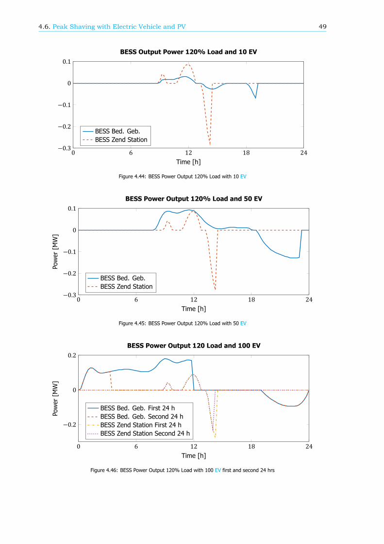
4.6. Peak Shaving with Electric Vehicle and PV 49
0 6 12 18 24−0.3
−0.2
−0.1
0
0.1
Time [h]
BESS Output Power 120% Load and 10 EV
BESS Bed. Geb.BESS Zend Station
Figure 4.44: BESS Power Output 120% Load with 10 EV
0 6 12 18 24−0.3
−0.2
−0.1
0
0.1
Time [h]
Power
[MW]
BESS Power Output 120% Load and 50 EV
BESS Bed. Geb.BESS Zend Station
Figure 4.45: BESS Power Output 120% Load with 50 EV
0 6 12 18 24
−0.2
0
0.2
Time [h]
Power
[MW]
BESS Power Output 120 Load and 100 EV
BESS Bed. Geb. First 24 hBESS Bed. Geb. Second 24 hBESS Zend Station First 24 hBESS Zend Station Second 24 h
Figure 4.46: BESS Power Output 120% Load with 100 EV first and second 24 hrs
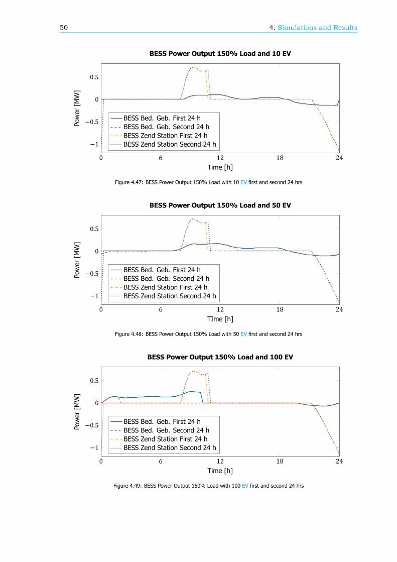
50 4. Simulations and Results
0 6 12 18 24
−1
−0.5
0
0.5
Time [h]
Power
[MW]
BESS Power Output 150% Load and 10 EV
BESS Bed. Geb. First 24 hBESS Bed. Geb. Second 24 hBESS Zend Station First 24 hBESS Zend Station Second 24 h
Figure 4.47: BESS Power Output 150% Load with 10 EV first and second 24 hrs
0 6 12 18 24
−1
−0.5
0
0.5
TIme [h]
Power
[MW]
BESS Power Output 150% Load and 50 EV
BESS Bed. Geb. First 24 hBESS Bed. Geb. Second 24 hBESS Zend Station First 24 hBESS Zend Station Second 24 h
Figure 4.48: BESS Power Output 150% Load with 50 EV first and second 24 hrs
0 6 12 18 24
−1
−0.5
0
0.5
Time [h]
Power
[MW]
BESS Power Output 150% Load and 100 EV
BESS Bed. Geb. First 24 hBESS Bed. Geb. Second 24 hBESS Zend Station First 24 hBESS Zend Station Second 24 h
Figure 4.49: BESS Power Output 150% Load with 100 EV first and second 24 hrs
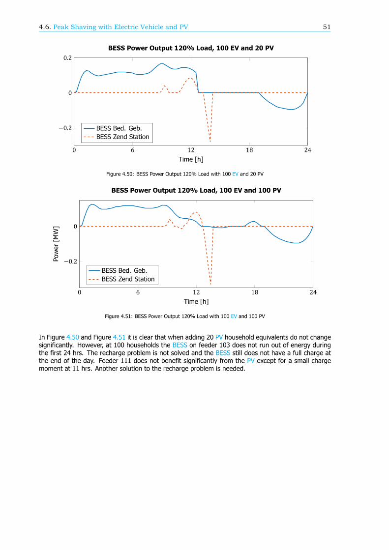
4.6. Peak Shaving with Electric Vehicle and PV 51
0 6 12 18 24
−0.2
0
0.2
Time [h]
BESS Power Output 120% Load, 100 EV and 20 PV
BESS Bed. Geb.BESS Zend Station
Figure 4.50: BESS Power Output 120% Load with 100 EV and 20 PV
0 6 12 18 24
−0.2
0
Time [h]
Power
[MW]
BESS Power Output 120% Load, 100 EV and 100 PV
BESS Bed. Geb.BESS Zend Station
Figure 4.51: BESS Power Output 120% Load with 100 EV and 100 PV
In Figure 4.50 and Figure 4.51 it is clear that when adding 20 PV household equivalents do not changesignificantly. However, at 100 households the BESS on feeder 103 does not run out of energy duringthe first 24 hrs. The recharge problem is not solved and the BESS still does not have a full charge atthe end of the day. Feeder 111 does not benefit significantly from the PV except for a small chargemoment at 11 hrs. Another solution to the recharge problem is needed.


5Conclusions and Recommendations
In the previous chapter the results of the various simulation scenarios based on the research objectivesestablished in Chapter 2 were presented and analyzed. In this chapter the conclusions are set out thatcan be drawn from the simulations results, and a series of suggested recommendations are made forfurther research regarding EES for MV Networks.
5.1. ConclusionsThe results of the various simulations contained in the previous chapter have been analyzed and theresults are discussed below. These results were obtained from the simulations performed on the nine-bus system and on the grid model based on the network of Stellendam using the scenarios and theiraccompanying variables described in Chapter 3. After an examination and analysis of these results, itis possible to determine if the effects on the grid meet the expectations and if these results answer thequestions posed in Section 2.7.
5.1.1. Conclusions of Reference Case SimulationThe nine-bus system was used in order to test the peak shaving algorithm that was presented inChapter 4. Simulation results were obtained from this grid using the household load profile on itssingle load. From these simulation results it was clear that the algorithm had the expected and desiredeffects. This was visible in the clear drop in cable load compared to the situation without peak shaving,seen in Figure 4.3, when the MCL is reached. From the results it is also possible to conclude that theBESS model created inChapter 3 works properly. This is can be observed by the BESS’s capability torecharge after being used and an indicated drop in its SoC. The peak shaving algorithm works in thissimplified network and therefore it is possible to continue with the more complex real world scenario.
5.1.2. Conclusions of Feeder 103Feeder 103 is the one with the BESS connected at busbar Bed. Geb. and the one that has a relativelylow power demand. The MCL and MRCL where therefore set at low values: 9% and 8% respectively.Feeder 103 is a radial network, as a consequence no abnormal behavior was expected when peakshaving at the busbar Bed. Geb. However, when examining the results obtained from the simulationsunder the different scenarios that were run, there are several results that standout.
Until the scenario 200% consumer load is reached, the BESS has no trouble coping with the increasedload during peak demand. Having a low power output compared to the maximum allowed increasesthe time the BESS can output power. As a result the BESS has enough energy to peak shave all peaksand recharge the BESS in all three scenarios. However, the scenario with 200% consumer incidencedoes pose a problem. Due to the increase the MCL is met sooner and the MRCL is reached later,resulting in more energy being required. This has the effect of less energy being charged. However,this situation can easily be remedied by increasing the MCL and MRCL, as these values are low whencompared to feeder 111. The only negative consequence of this solution is an increase in cable losses.An alternative solution would be to change the default SoC to 60% instead of 50%. This would add an
53

54 5. Conclusions and Recommendations
additional 10% increase in available energy, while at the same time reducing the capability of the BESSto handle excess power on the grid. This could create a problem if large amounts of PV are present onthe network. A final solution would be to increase the overall storage size of the BESS. However, thissolution will make it a more expensive investment decision and, therefore, may be a less cost-effectivesolution when compared with upgrading other network components.
Table 5.1: Feeder 103 cable losses results
Scenario w\o BESS w\ BESS Saved
120% Load 11.23 kWh 11.24 kWh 0%150% Load 15.97 kWh 15.06 kWh 5.7%200% Load 26.32 kWh 22.16 kWh 15.8%
It is obvious on feeder 103 that peak shaving has the expected effects of lowering cable load and cablelosses. Table 5.1 provides an overview of the cable losses results per scenario. The voltage deviationon the busbar is also reduced, but not by a significant amount. These voltages per scenario are shownin Table 5.2. These results imply that voltage control would be a better solution if the voltage deviationbecomes a problem at increased loads.
Table 5.2: Feeder 103 busbar voltages results
Scenario w\o BESS w\ BESS
120% Load 0.9930 pu 0.9932 pu150% Load 0.9902 pu 0.9908 pu200% Load 0.9851 pu 0.9863 pu
The addition of EV to feeder 103 is a relatively large increase when comparing it to the addition of EVto feeder 111. The load is increased by 37 kW, 185 kW and 370 kW which translates to a 7%, 35.2%,and 70.4% load increases, respectively, when compared to the original load of 525.35 kW. Therefore,it is not surprising that the BESS has more trouble coping with the peaks because of this increase. Dueto EV charging at night, more peaks are created during this time period which has as its consequencenot only a power demand increase, but also a total energy demand increase from the BESS. This hastwo effects on the BESS.
First, the BESS runs out of energy sooner and is not able to fully recharge before the next cycle,which results in depleting the available energy in the BESS. This is a clear problem in the three sce-narios: 120% consumer load and 100 EV; 150% consumer load and 50 EV; and 150% consumer loadand 100 EV.
Second, the MCL is reached during EV charging at night which causes the BESS to start discharg-ing earlier. As the BESS energy supply is limited to 15 kWh, it runs out of energy with the result beingan insufficient level of energy for the rest of the day.
These problems do not have a straight forward solution because the added load profile creates anadditional peak in the morning, increasing the need for energy while at the same time decreasing thecapability of the BESS to store energy. Increasing the available energy by changing the default SoCor increasing the BESS size will not solve the recharge problem. Therefore, it would appear that anincrease of the MCL and MRCL is the most straight-forward option. This can be accomplished by ad-justing the MCL and MRCL to accommodate for the new peak formed by the added EV.
When observing the scenario with added PV, it is obvious that introducing a large amount of PV has apositive effect on the capabilities of the BESS. As the PV is an extra source of energy, the size of thepeak during PV energy generation is reduced. The network requires less energy from the BESS, andat 13 hrs is able to recharge slightly due to the excess amount of energy produced by the PV. As aconsequence, adding PV would appear to be a valid option to solve the growing amount of EV.

5.1. Conclusions 55
Table 5.3: Feeder 111 cable losses results
Scenario w\o BESS w\ BESS Saved
120% Load 1719.7 kWh 1721.6 kWh 0%150% Load 2774.5 kWh 2700.7 kWh 2.7%200% Load 5228.0 kWh 4144.9 kWh 20.7%
5.1.3. Conclusions of Feeder 111Feeder 111 is a high energy demand feeder, and its configuration is comparable to feeder 103 as it alsohas a radial configuration. Due to its size, the values of the MCL and MRCL were set higher than thoseof feeder 103, at 55% and 50%, respectively. The BESS was connected to the busbar Zend Station.The results of the simulations were similar to those of feeder 103 with one exception. Due to the largeenergy demand of feeder 111, the BESS runs out of energy far more quickly when faced with highpeaks. This is clearly evident in the scenarios 150% and 200% consumer size. Again the solution forthis problem is to alter the MCL and MRCL, alter the BESS size, or alter the SoC default value. Resultsfor cable loading, cable losses and busbar voltage are similar to those of feeder 103. The results arepresented in Table 5.3 and Table 5.4.
Adding EV to this feeder does not have the same impact as it does on feeder 103. This can be explainedby the large energy consumption of feeder 111. The addition to EV is a relative small increase whencompared with the increase it causes in feeder 103. For feeder 111 the load is increased with the sameamount as with feeder 103. The relative size increases are for feeder 111: 0.08%, 3.9% and 7.8%. Forthis reason feeder 111 does not show additional problems when compared with the scenario without EV.
An identical situation occurs with the addition of PV. The relative small addition in power has a smalleffect on feeder 111. It is only just visible where adding 100 households when an extra charge momentoccurs at 11 hrs.
Table 5.4: Feeder 111 busbar voltages results
Scenario w\o BESS w\ BESS
120% Load 0.9560 pu 0.9573 pu150% Load 0.9429 pu 0.9544 pu200% Load 0.9230 pu 0.9506 pu
5.1.4. Conclusions of Feeder 204Feeder 204 is the feeder that has a relative low power demand and its radial configuration posed prob-lems during the simulations. In the scenarios the MCL and MRCL were set at 9% and 8%. Whenlooking at the results of peak shaving, the effect is not what is anticipated. Instead of a straight lineduring BESS operation, a curved line in the shape of the load profile was observed at a lower load. Thisindicates that instead of shaving the peak the load is overall reduced. This problem occurred in themeshed configuration. It was possible to eliminate this problem by using the “power” component ofthe cables instead of the “current” component within PowerFactory. This solution did not work for theradial configuration and a deeper insight into the definition of the elements compromising the variablesavailable in PowerFactory is required to find a solution to this problem.
Even though peak shaving was not accomplished properly, losses and loading were reduced on thecables. This partial result appears to indicate that, if peak shaving can be implemented properly, thesame effects are to be expected as on the meshed configured feeders. However, in the model it isonly possible to limit the load on one cable at a time with the current peak shaving method. A morecomplex peak shaving method could be implemented to limit the load on both incoming cables. Thisconfiguration will pose a challenge as there are two parameters which are dependent upon one anotherto be controlled with one system.

56 5. Conclusions and Recommendations
Overall it can be concluded that under the conditions set out in the simulations models peak shav-ing on this MV voltage grid has the expected and desired effects. Cable loads and cable losses weresuccessfully reduced. The successful provision of power supply capacity increase, congestion relief,transmission upgrade deferral, and distribution upgrade deferral can all be accomplished when using aBESS to peak shave. However, voltage support will be required for large increases in load in the futureas peak shaving does not sufficiently correct the voltage deviation.
With an increase in consumer consumption the size of the BESS and set limits of the MCL and MRCLwill remain adequate until a consumer increase of 50% is reached. Beyond this level the BESS size willhave to be increased, the limits of the MCL and MRCL adjusted or the the SoC default value increasedto improve available energy. These measures can be used until the network reaches its maximumtolerable load, at which point the network components will have to be replaced with ones that canhandle the increasing load.
An increase in EV has large negative effects on the BESS primarily by disrupting the ability of theBESS to recharge at night. This causes the BESS to run out of energy sooner during the next cycle.Adding PV under these circumstances improved the BESSs ability to cope with the increased EV, therebyremoving the need to install a larger BESS or to change the values of the MCL and MRCL.
5.2. RecommendationsFrom the conclusions and observations provided in the previous section several recommendations canbe made for future research in the subject of Electric Energy Storage in a Medium Voltage Grid. Theserecommendations are set out below.
• Further research on the effect of adding voltage control to the busbars to determine what influ-ence it has on cable loading, cable losses, and the operation of the BESS.
• Further research on the effect of providing a fix or work-around for the meshed feeder configu-ration in PowerFactory in order to check if the predictions that were made are correct.
• Expand the radial configured grid to limit the load on all incoming cables. This can be done usinga current limiter and measuring the phase angle.
• Further research into the effect of integrating several EESS technologies into one system, e.g.,peak shaving and voltage control.
• Solve the recharge problem when EV is added to the network by load scheduling the charging ofthe EV

AInternational Electrotechnical
Commission Standards
57

58 A. International Electrotechnical Commission Standards
A.1. Fire Hazard Testing – IEC 60695-1-11:2010This regulation specifies guidance for assessing the fire hazard of electrochemical products. It outlinesthe methods for choosing the best fire hazard testing and performance measures.
Fire hazard is a physical object or condition with a potential for an undesirable consequence fromfire.
Fire risk is calculated from the probability of fire and a quantified measure of its consequences.
Fire hazard assessment involves the assessment of the possible causes of fire, the possibility andnature of subsequent fire growth, and the possible consequences of fire.
A.2. Analysis Techniques for SystemReliability – IEC 60812:2006This regulation describes Failure Mode and Effects Analysis. The reasons for undertaking Failure ModeEffects Analysis (FMEA) or Failure Mode Effects and Criticality Analysis (FMECA) may include the fol-lowing:
1. to identify those failures which have unwanted effects on system operation, e.g. preclude orsignificantly degrade operation or affect the safety of the user;
2. to satisfy contractual requirements of a customer, as applicable;
3. to allow improvements of the system’s reliability or safety (e.g. by design modifications or qualityassurance actions);
4. to allow improvement of the system’s maintenance (by highlighting areas of risk or nonconformingmaintenance).
A.3. Fault Tree Analysis (FTA) – IEC 61025:2006This document describes the fault tree analysis and gives guidance on how to use it. FTA may beundertaken independently of, or in conjunction with, other reliability analyses.
Objectives include:
• identification of the causes or combinations of causes leading to the top event;
• determination of whether a particular system reliability measure meets a stated requirement;
• determination of which potential failure mode(s) or factor(s) would be the highest contributor tothe system probability of failure (unreliability) or unavailability, when a system is repairable, foridentifying possible system reliability improvements;
• analysis and comparison of various design alternatives to improve system reliability;
• demonstration that assumptions made in other analyses (such as Markov and FMEA) are valid;
• identification of potential failure modes that might cause a safety issue, evaluation of correspond-ing probability of occurrence and possibility of mitigation;
• identification of common events (e.g. the middle branch of a bridge circuit);
• search for an event or combinations of events which are the most likely to cause the top eventto occur;
• assessment of the impact of the occurrence of a primary event on the probability of the top event;
• calculation of event probabilities; and
• calculation of availabilities and failure rates of system or its components represented by a faulttree, if a steady state can be postulated, and eventual repairs are independent of each other(same limitation as for the success path diagram/reliability block diagram).

A.4. Protection from Electric Shock – IEC 61140:2002 59
Fault Tree Analysis is a deductive (top-down) method of analysis aimed at pinpointing the causes,or combinations of causes, that can lead to the defined top event. The analysis can be qualitative,Method A, or quantitative, Method B, depending on the scope of the analyses.
A.4. Protection from Electric Shock – IEC 61140:2002The regulation protecting humans and animals against electric shock is applicable for all systems andequipment. Hazardous-live-parts shall not be accessible and accessible conductive parts shall not behazardous live.
Basic protection provisions:
• Basic insulation
• Barriers or enclosures
• Obstacles
• Placing out of arms reach
• Limited voltage specified in IEC 61201
• Limited steady-state touch current and charge
• Potential grading
A.5. Batteries for Renewable Energy Storage – IEC 61427-1:2013Specifications for secondary batteries used in photovoltaic energy systems and gives test standardsused for the verification of battery performance. Batteries must satisfy the following requirements:
• mechanical endurance,
• charge efficiency, and
• deep charge protection.
Testing methods are:
• capacity test,
• generic cycling endurance test, and
• charge retention test.
Different specifications apply for different battery types.
A.6. Functional Safety of Programmable Safety Related SystemsIEC 61508
IEC 61508-1:1998 – Part 1: General requirements.
IEC 61508-2:2000 – Part 2: Requirements for electrical/electronic/programmable electronic safety-related systems.
IEC 61508-3:1998 – Part 3: Software requirements.
IEC 61508-4:1998 – Part 4: Definitions and abbreviations.
IEC 61508-5:1998 – Part 5: Examples of methods for the determination of safety integrity levels.
IEC 61508-6:2000 – Part 6: Guidelines on the application of IEC 61508-2 and IEC 61508-3.

60 A. International Electrotechnical Commission Standards
IEC 61508-7:2000 – Part 7: Overview of techniques and measures.
Functional safety is part of the overall safety that depends on a system or equipment operating correctlyin response to its inputs.
A.7. Safety of LithiumBatteries During Transport – IEC 62281:2013This regulation provides safety requirements for transport of lithium cells and batteries. The followingdesign concepts for safety are common to all lithium cells and batteries:
• Abnormal temperature rise above the critical value defined by the manufacturer shall be preventedby design.
• Temperature increases in the cell or battery shall be controlled by the design, e.g. by limiting thecurrent flow.
• Lithium cells and batteries shall be designed to relieve excessive internal pressure or to precludea violent rupture under conditions of transport.
• Lithium cells and batteries shall be designed so as to prevent a short-circuit under normal condi-tions of transport and intended use.
• Lithium batteries containing cells or strings of cells connected in parallel shall be equipped witheffective means, as may be necessary, to prevent dangerous reverse current flow (e.g., diodes,fuses, etc.).
Lithium cells and batteries shall be packaged so as to prevent an external short-circuit under normaltransport conditions.
A battery assembly with aggregate lithium content of more than 500 g, or in the case of a lithiumion battery, with a nominal energy of more than 6,200 Wh, does not need to be tested if:
• it is formed by electrically connecting batteries that have passed all applicable tests, and
• it is equipped with a system capable of:
– monitoring the battery assembly,
– preventing short-circuits and over-discharge between the batteries in the assembly, and
– preventing any overheat or overcharge of the battery assembly.
A.8. Environmentally Conscious Design – IEC 62430:2009Environmentally conscious design shall be based on the concept of Life Cycle Thinking (LCT), whichrequires consideration during the design and development process of the significant environmentalaspects of a product in all life cycle stages. Key elements of Life Cycle Thinking are as follows:
• having an objective to minimize the overall adverse environmental impact of the product;
• identifying, qualifying and where feasible, quantifying the significant environmental aspects ofthe product; and
• considering the trade-offs between environmental aspects and life cycle stages.
The above shall be initiated as early as possible in the design and development process, when mostopportunities exist to make changes and improvements to the product affecting its overall environmen-tal performance throughout its life cycle.
Organizations performing Environmentally Conscious Design (ECD) shall establish, document, imple-ment and maintain an ECD process as an integral part of the product design and development process.This ECD process includes the following steps:

A.9. Safety Requirements for Battery Installations – IEC 62485-2:2010 61
• analysis of the regulatory and stakeholders’ environmental requirements;
• identification and evaluation of environmental aspects and corresponding impacts;
• design and development;
• review and continual improvement.
The organization shall, while following the above steps, document the relevant results and the subse-quent conclusions and responsibilities assigned.
A.9. Safety Requirements for Battery Installations – IEC 62485-2:2010
In battery installations, protection against direct contact with live parts shall be ensured in accordancewith IEC 60364-4-41. The following protective measures apply:
• “protection by insulation of live parts”;
• “protection by barriers or enclosures”;
• “protection by obstacles”;
• “protection by placing out of reach”.
In battery installations, protection against indirect contact shall be applied in accordance with IEC 60364-4-41. One or more of the following measures shall be selected:
• “protection by automatic disconnection of supply”;
• “protection by use of class II equipment or by equivalent insulation”;
• “protection by non-conducting locations” (used in specific applications only);
• “protection by earth-free local equipotential bonding” (used in specific applications only);
• “protection by electrical separation”.
Devices shall be provided to disconnect the battery installation from all lines of incoming and outgoingcircuits and from earth potential. These devices can be:
• circuit breakers, switches;
• plug and socket outlets;
• removable fuses;
• connecting links;
• specially designed clamps.


BDigSILENT PowerFactory Nine-bus
System
63

Nine-bus System
DIgSILENT PowerFactory ∗
Abstract
This paper describes the Nine-bus System,which was introduced in the book PowerSystem Control and Stability by P. M. An-derson and A. A. Fouad [1]. The parame-ters of the individual elements like genera-tors, loads, transformers and lines, as well asthe adaptation of their values for input in thePowerFactory network model are explained.Results for the load flow calculation and sta-bility simulation (dynamic RMS phasor simu-lation) obtained with the Nine-bus System inPowerFactory are presented.
1 General Description
The Nine-bus System was introduced in thebook Power System Control and Stability byP. M. Anderson and A. A. Fouad [1]. It rep-resents a small transmission system whichconsists of 9 buses (nodes), 3 generators, 3loads, 6 lines and 3 transformers, the singleline diagram is shown in Figure 1.
2 Model Parameters
The nominal voltage of the transmissionsystem is 230 kV, the nominal frequency is60 Hz. The following subsections describethe parameters of the elements as used forbalanced load flow calculation and RMS sim-ulation. Data have been taken from [1].
∗DIgSILENT GmbH, Heinrich-Hertz-Str. 9, 72810Gomaringen, Germany, www.digsilent.de
2.1 Loads
During load flow calculation, the loads ofthe Nine-bus System have constant activeand reactive power demand [1], they arenot voltage-dependent. This is achieved bydisabling the load option “Consider VoltageDependency of Loads” in the PowerFactoryload flow calculation command.
Load data (active power P and reactivepower Q) are listed in Table 1.
The steady-state load flow determines theinitial values for the stability simulation (dy-namic RMS phasor simulation). DuringRMS simulation the loads are considered asequivalent impedances.
2.2 Generators
Generator “G1” is the slack machine, volt-age 1.04 p.u. and 0 degrees. The othergenerators are configured to control the ac-tive power injection and voltage magnitudesat the connected buses, therefore the activepower dispatch and controlled voltage mag-nitudes at their terminals are given.
The data have been taken from [1] and arelisted in Table 2 and 4.
The reactances x of the generators havebeen adapted to the generator rated powerSr,gen using Equation 1. The inertia timeconstant H based on the rated active powerPr,gen has been calculated from the storedenergy E at nominal speed with Equation 2.The results are presented in Table 3.
DIgSILENT PowerFactory, r2752 1

Nine-bus System
Figure 1: Single line diagram of the Nine-bus System
x[p.u.generator base] (1)
= x[p.u.system base] ·Sr,gen[MVA]
100 MVA
H =E
Pr,gen(2)
For RMS simulation, two dynamic modelsfor synchronous generators are available inPowerFactory 15.2: a classical and a de-tailed model. The detailed model representsa field winding in the d-axis, and a damperwinding in the d- and q-axis [2]. The classi-cal model is a simplified model consisting ofa voltage source behind an impedance [2].To reproduce the examples described in [1],both models are used in accordance to [1].
2.3 Transmission Lines
Line data are given in per unit (p.u.) on aSb = 100 MVA system base as representedin Table 6 [1]. As there is no line length givenin [1], the length of each line in the Power-Factory model has been set to 1 km.
For the PowerFactory model input data arerequired in Ω/km and µF/km respectively.Line data have been recalculated for the net-work model with the nominal voltage Un =230 kV using Equations (3) – (5).
R [Ω] = r [p.u.] · U2n [kV2]
Sb [MVA](3)
X [Ω] = x [p.u.] · U2n [kV2]
Sb [MVA](4)
B [µS] = b [p.u.] ·Sb [MVA]
U2n [kV2]
· 10−6 (5)
Lines are assumed to be overhead lines andsince the rated current of each line is notknown, it is assumed to be 1 kA.
2.4 Transformers
Transformer data are given in per unit (p.u.)on a 100 MVA system base as representedin Table 7 [1]. In the PowerFactory model,the rated power of the transformers has beenchosen according to the size of the con-nected generators. The reactances x of
DIgSILENT PowerFactory, r2752 2

Nine-bus System
the transformers have been adapted to thetransformer rated power Sr,trf using Equa-tion 6. Transformer parameters of the Pow-erFactory model are given in Table 8.
x[p.u.transformer base] (6)
= x[p.u.system base] ·Sr,trf [MVA]
100 MVA
The vector group of all transformers hasbeen assumed to be YNd5. This leads to anadditional phase shift of 150 degrees for thevoltage angles at the 230 kV level in the Pow-erFactory results compared to the results ob-tained in [1].
3 Load Flow Results
The steady-state load flow is examined byexecuting the load flow calculation ( ). Theresults of the PowerFactory load flow calcu-lation are depicted in Figure 2 and addition-ally provided in Appendix B.
4 RMS Simulations
A number of different RMS simulations isperformed to analyse the transient stability ofthe Nine-bus System and the effect of differ-ent excitations systems and of a power sys-tem stabiliser.
4.1 Five Cycles Fault
In this study case the Example 2.7 of thebook Power System Control and Stability [1]is reproduced. In this example the classicalsynchronous generator model is used as de-scribed in [1]. In order to reproduce the clas-sical model described in the book (section2.5.1) the transient reactance x′d is used asstator reactance (xstr) in the PowerFactorymodel.
A three-phase short-circuit event is simu-lated at an end of the Line 5-7. The faultis cleared in five cycles (83.3 ms) by trippingthe faulted line.
The resulting curves for the rotor angles ofgenerators “G2” and “G3” with reference to“G1” are shown in Figure 3. The rotor anglesof both generators reach a maximum valueand then decrease. Transient stability of thesystem is given in this scenario. The resultscorrespond with [1].
4.2 Impact of the Excitation Sys-tem
This simulation described in Section 4.1 wascarried out without any controller taken intoaccount. However, in a real system the con-trols have a big impact on the stability of thesystem. In the following study cases with dif-ferent types of excitation systems are pre-sented. In these cases the detailed syn-chronous machine model is used, which al-lows to connect an excitation system (auto-matic voltage regulator, AVR) to the genera-tor.
The following types of the excitation systemare modelled at the generator G2, in order toreproduce results provided in [1]:
• Detailed model of the synchronous ma-chine available in PowerFactory (no ad-ditional control)
• Detailed model of the synchronous ma-chine with an AVR model IEEE type 1Amplidyne
• Detailed model of the synchronous ma-chine with an AVR model IEEE type 1Mag-A-Stat
• Detailed model of the synchronous ma-chine with an AVR model IEEE type 3SCPT
The excitation models are taken from theglobal library available in PowerFactory andthe parameter values are modified accord-ing to the data provided in [1]. A three-phasefault with a duration of three cycles (50 ms) issimulated at the end on the Line 5-7, the faultis cleared by tripping the faulted line. The re-sults are depicted in Figure 4.
The results show good consistence with [1].The maximum rotor angle differs dependingon the AVR type used. This demonstrates
DIgSILENT PowerFactory, r2752 3

Nine-bus System
the effect which the excitation system hason the transient stability of the generator.The smaller the maximum rotor angle is, thelarger is the margin to the stability limit.
4.3 Impact of an Power SystemStabiliser
In order to simulate the impact of the PowerSystem Stabiliser (PSS), a PSS model asspecified in [1] is added to the control of themachine. The PSS model is taken from theglobal library available in PowerFactory andthe parameter values are chosen accordingto the data provided in [1]. The case withthe AVR model IEEE type 1 Mag-A-Stat wasused for this study. Results are shown in Fig-ure 5 and Figure 6. The PSS damps the os-cillation of the generator by influencing theexcitation voltage.
References
[1] P. Anderson and A. Fouad, Power Sys-tem Control and Stability, 1st ed. IowaState University Press, Ames, Iowa,U.S.A., 1977.
[2] DIgSILENT PowerFactory 15.2: Tech-nical Reference Documentation Syn-chronous Machine, Version 15.2, 1st ed.,DIgSILENT GmbH, Heinrich-Hertz-Str.9, 72810 Gomaringen, Germany, 2015.
DIgSILENT PowerFactory, r2752 4

Nine-bus System
Figure 2: Results of the load flow calculation
Figure 3: Rotor Angle with reference to the reference machine
DIgSILENT PowerFactory, r2752 5
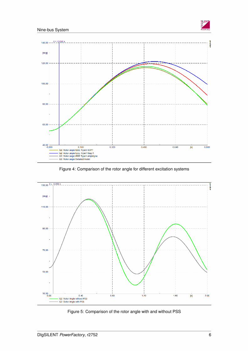
Nine-bus System
Figure 4: Comparison of the rotor angle for different excitation systems
Figure 5: Comparison of the rotor angle with and without PSS
DIgSILENT PowerFactory, r2752 6

Nine-bus System
Figure 6: Comparison of the excitation voltage with and without PSS
A Tables with Input Data
Table 1: Load demand [1]
Load Bus P [MW] Q [Mvar]Load A Bus 5 125 50Load B Bus 6 90 30Load C Bus 8 100 35
DIgSILENT PowerFactory, r2752 7

Nine-bus System
Table 2: Generator Data (x based on 100 MVA) [1]
Quantity G1 G2 G3Nominal apparent power [MVA] 247.5 192.0 128.0Nominal voltage [kV] 16.5 18.0 13.8Nominal power factor 1.00 0.85 0.85Type hydro steam steamNominal speed [rpm] 180 3600 3600xd [p.u.] 0.1460 0.8958 1.3125x′d [p.u.] 0.0608 0.1198 0.1813xq [p.u.] 0.0969 0.8645 1.2578x′q [p.u.] 0.0969 0.1969 0.2500xl (leakage) [p.u.] 0.0336 0.0521 0.0742τ ′d0 [s] 8.960 6.000 5.890τ ′q0 [s] 0.000 0.535 0.600
Stored energy at nominal speed [MW · s] 2364 640 301
Table 3: Generator Data in the PowerFactory model (x based on rated power)
Quantity G1 G2 G3Nominal apparent power [MVA] 247.5 192.0 128.0Nominal voltage [kV] 16.5 18.0 13.8Nominal power factor 1.00 0.85 0.85Plant Category Hydro Coil CoilRotor Type salient pole round rotor round rotorxd [p.u.] 0.3614 1.7199 1.6800x′d [p.u.] 0.1505 0.2300 0.2321xq [p.u.] 0.2328 1.6598 1.6100x′q [p.u.] - 0.3780 0.3200xl (leakage) [p.u.] 0.0832 0.1000 0.0950τ ′d0 [s] 8.960 6.000 5.890τ ′q0 [s] - 0.535 0.600
Inertia Constant H (Rated to Pgn) [s] 9.5515 3.9216 2.7665
Table 4: Generator dispatch and voltage setpoints [1]
Generator Bus P [MW] u [p.u.]G1 Bus 1 N/A 1.040G2 Bus 2 163.0 1.025G3 Bus 3 85 1.025
DIgSILENT PowerFactory, r2752 8

Nine-bus System
Table 5: Data of lines based on 100 MVA [1]
From To r [p.u.] x [p.u.] b/2 [p.u.]Bus 4 Bus 5 0.0100 0.0850 0.0880Bus 4 Bus 6 0.0170 0.0920 0.0790Bus 5 Bus 7 0.0320 0.1610 0.1530Bus 6 Bus 9 0.0390 0.1700 0.1790Bus 7 Bus 8 0.0085 0.0720 0.0745Bus 8 Bus 9 0.0119 0.1008 0.1045
Table 6: Data of lines in the PowerFactory model
Line From To R [Ω] X [Ω] B [µS]Line 4-5 Bus 4 Bus 5 5.2900 44.9650 332.70Line 4-6 Bus 4 Bus 6 8.9930 48.6680 298.69Line 5-7 Bus 5 Bus 7 16.928 85.1690 578.45Line 6-9 Bus 6 Bus 9 20.631 89.9300 676.75Line 7-8 Bus 7 Bus 8 4.4965 38.0880 281.66Line 8-9 Bus 8 Bus 9 6.2951 53.3232 395.08
Table 7: Data of transformers based on 100 MVA [1]
Transformer From To Ur HV [kV] Ur LV [kV] x1 [p.u.]T1 Bus 1 Bus 4 230 16.5 0.0576T2 Bus 2 Bus 7 230 18.0 0.0625T3 Bus 3 Bus 9 230 13.8 0.0586
Table 8: Data of transformers in the PowerFactory model
Transformer From To Rated Power [MVA] Ur HV [kV] Ur LV [kV] x1 [p.u.]T1 Bus 1 Bus 4 250 230 16.5 0.1440T2 Bus 2 Bus 7 200 230 18.0 0.1250T3 Bus 3 Bus 9 150 230 13.8 0.0879
DIgSILENT PowerFactory, r2752 9

Nine-bus System
B Tables with Results of the Balanced Load Flow Calculation
Table 9: Results of bus voltages provided in [1]
Name u, Magnitude u, Angle[p.u.] [deg]
Bus 1 1.040 0.0Bus 2 1.025 9.3Bus 3 1.025 4.7Bus 4 1.026 -2.2Bus 5 0.996 -4.0Bus 6 1.013 -3.7Bus 7 1.026 3.7Bus 8 1.016 0.7Bus 9 1.032 2.0
Table 10: Results of bus voltages obtained with PowerFactory
Name U, Magnitude (line-line) u, Magnitude u, Angle (line-earth)[kV] [p.u.] [deg]
Bus 1 17.16 1.040 0.00Bus 2 18.45 1.025 9.25Bus 3 14.15 1.025 4.64Bus 4 235.96 1.025 147.78 = 150.00 - 2.22Bus 5 229.07 0.996 146.02 = 150.00 - 3.98Bus 6 232.95 1.013 146.31 = 150.00 - 3.69Bus 7 235.97 1.026 153.69 = 150.00 + 3.69Bus 8 233.69 1.016 150.70 = 150.00 + 0.70Bus 9 237.48 1.033 151.95 = 150.00 + 1.95
Table 11: Results of generators provided in [1]
Name Active Power Reactive Power[MW] [Mvar]
G1 71.6 27.0G2 163.0 6.7G3 85.0 -10.9
Table 12: Results of generators obtained with PowerFactory
Name Active Power Reactive Power[MW] [Mvar]
G1 71.60 26.78G2 163.00 6.70G3 85.00 -10.90
DIgSILENT PowerFactory, r2752 10

Nine-bus System
Table 13: Results of lines
Name Losses Reactive Losses Capacitive Loading[MW] [Mvar] [Mvar]
Line 4-5 0.2551 -15.8229 17.9913Line 4-6 0.1675 -15.5132 16.4196Line 5-7 2.2969 -19.8453 31.4014Line 6-9 1.3477 -31.5696 37.4443Line 7-8 0.4735 -11.5217 15.5328Line 8-9 0.0885 -21.1783 21.9284
DIgSILENT PowerFactory, r2752 11

CSingle Line Diagrams
75

76 C. Single Line Diagrams
Figure C.1: Vision Single Line Diagram of the Grid Model
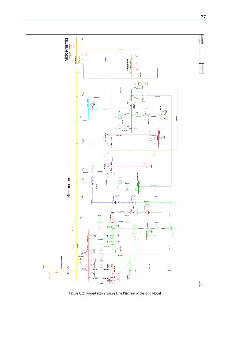
77
Figure C.2: PowerFactory Single Line Diagram of the Grid Model


DCode
79

80 D. Code
1 object ldf , setTime , oGrb , oViPg , oPlot , oGrb2 , oViPg2 , oPlot2 , oPlot3 , oViPg3 , oPlot4 , ...oPlot5 , oViPg4 , oPlot6 , oPlot7 ;
2 int i , steps , error , j , k , time , time_step ;3 double over_current1 , max_cable1_current , rated_current_3x30 , p_battery , cable1_current , ...
cable2_current , over_current2 , over_current ;4 double SoCn, SoCo , SoC_diff , SoCn2 , SoCo2 , SoC2_diff , load , load2 , bus_current , ...
bus_current2 , p_battery2 , under_current , under_current2 ;5 double cable1load , cable2load , cable5load , max_power1 , max_power2 , done , done2 ;6 double battery1_empty , battery2_empty , min_power1 , min_power2 , done3 , done4 ;7 double battery3_empty , cable6load , done5 , done6 , max_power3 , min_power3 ;8 double load3 , bus_current3 , over_current3 , under_current3 , p_battery3 ;9 double SoCn3 , SoC3 , SoCo3 , SoC3_diff , over_load2 ;
10 object oPlot8 , oPlot9 , oViPg5 , oPlot10 , Time ;11 double max_current , min_current , max_current2 , min_current2 , max_current3 , min_current3 ;12 double ZSLoad , hour , battery_step ;13
14 ClearOutput () ;15 Results . Clear () ;16 EchoOff ( ) ;17
18 ! I n i t i l i z e var iab le s19 i = 0;20 steps = 96;21 k = 0;22 time_step = 150000;23 time = 0;24 battery_step = 4;25 setTime = GetCaseObject ( ’SetTime ’ ) ;26 setTime : cDate = 20160318;27 setTime : cTime = 0000000;28 hour = 0;29 SoC = 0 .5 ;30 SoCn = SoC;31 SoCo = SoC;32 SoC2 = 0 . 5 ;33 SoCn2 = SoC2 ;34 SoCo2 = SoC2 ;35 SoC3 = 0 . 5 ;36 SoCn3 = SoC3 ;37 SoCo3 = SoC3 ;38 battery : pgini = 0;39 battery2 : pgini = 0;40 battery3 : pgini = 0;41 rated_current_3x30 = 3x50_cable_type : s l i n e ;42 done = 0;43 done2 = 0;44 done3 = 0;45 done4 = 0;46 done5 = 0;47 done6 = 0;48 battery1_empty = 0;49 battery2_empty = 0;50 battery3_empty = 0;51 max_power1 = 10000;52 max_power2 = 10000;53 max_power3 = 10000;54 min_power1 = -10000;55 min_power2 = -10000;56 min_power3 = -10000;57 max_current = 10000;58 min_current = -10000;59 max_current2 = 10000;60 min_current2 = -10000;61 max_current3 = 10000;62 min_current3 = -10000;63
64 PVS:ngnum = PV;65 PVS: outserv = o f f ;66
67 BGPV:ngnum = PV;68 BGPV: outserv = o f f ;

81
69
70 ! Loads71 PZ1: p l i n i = 0.974 * factor ;72 PZ2: p l i n i = 0.387 * factor ;73 PZ3: p l i n i = 0.532 * factor ;74 PZ4: p l i n i = 0.184 * factor ;75
76 BG1: s l i n i = 553 * factor ;77 BG2: s l i n i = 193 * factor ;78 BG3: s l i n i = 34 * factor ;79
80 ZS1 : s l i n i = 756 * factor ;81 ZS2 : s l i n i = 392 * factor ;82 ZS3 : p l i n i = 0.31 * factor ;83 ZS4 : s l i n i = 249 * factor ;84 ZS5 : s l i n i = 120 * factor ;85 ZS6 : s l i n i = 241 * factor ;86 ZS7 : s l i n i = 321 * factor ;87 ZS8 : s l i n i = 218 * factor ;88 ZS9 : s l i n i = 355 * factor ;89 ZS10 : s l i n i = 590 * factor ;90 ZS11 : s l i n i = 1170 * factor ;91
92 EVBG: p l i n i = ev * 0.0037;93 EVZS: p l i n i = ev * 0.0037;94
95 l d f = GetCaseObject ( ’ComLdf ’ ) ;96
97 max_current = 0.145* sqrt (3) * ( top_load_port/100) ;98 max_current2 = 0.145* sqrt (3) * ( top_load_bed/100) ;99 max_current3 = 0.22* sqrt (3) * ( top_load_zs/100) ;
100
101 min_current = 0.145* sqrt (3) * (bottom_load_port/100) ;102 min_current2 = 0.145* sqrt (3) * (bottom_load_bed/100) ;103 min_current3 = 0.22* sqrt (3) * (bottom_load_zs/100) ;104
105 ! Simulate multiple loadf lows106 while ( i<steps )107 108 i f (k=battery_step )109 110 hour += 1000000;111 time = hour ;112 setTime : cTime = time ;113 k = 0;114 115
116 error = ld f . Execute () ;117
118 i f ( e r ror )119 120 pr in t f ( ’ Error in loadflow ’ ) ;121 ex i t ( ) ;122 123
124 over_current = ( portzelande :m: Pout - ( cable2 :m:P: bus1 + ...cable2 :m:P: bus2 ) ) /(13* portzelande :m:u) - max_current ;
125 over_current2 = (bed :m: Pout - BGPV:m:P: bus1 ) /(13*bed :m:u) - max_current2 ;126 over_current3 = ( zs :m: Pout - PVS:m:P: bus1 ) /(13* zs :m:u) - max_current3 ;127
128 under_current = ( portzelande :m: Pout + battery : pgini - ( cable2 :m:P: bus1 + ...cable2 :m:P: bus2 ) ) /(13* portzelande :m:u) - min_current ;
129 under_current2 = (bed :m: Pout + battery2 : pgini - BGPV:m:P: bus1 ) /(13*bed :m:u) - min_current2 ;130 under_current3 = ( zs :m: Pout + battery3 : pgini - PVS:m:P: bus1 ) /(13* zs :m: u) - min_current3 ;131
132 i f ( over_current > 0)133 134 p_battery = (13 * portzelande :m:u * over_current ) ;135
136 SoCn = ((SoCo*battery_port ) -( p_battery/battery_step ) )/battery_port ;137

82 D. Code
138 i f ( p_battery>3)139 140 p_battery = 3;141 SoCn = ((SoCo*battery_port ) -( p_battery/battery_step ) )/battery_port ;142 143
144 i f (SoCn 0 . 4 . and . battery1_empty = 0)145 146 SoC_diff = 0.4 - SoCn;147 p_battery = SoC_diff * battery_port ;148 SoCn = 0 . 4 ;149 battery1_empty = 1;150 151 i f (SoCn 0 . 4 . and . battery1_empty = 1)152 153 p_battery = 0;154 SoCn = 0 . 4 ;155 156 157 e l s e i f ( over_current < 0. and . under_current < 0. and .SoC < 0.5)158 159 p_battery = (13 * portzelande :m:u * under_current ) ;160 SoCn = ((SoCo*battery_port ) -( p_battery/battery_step ) )/battery_port ;161 battery1_empty = 0;162 163 e l s e164 165 p_battery = 0;166 167
168 i f ( over_current2> 0)169 170 p_battery2 = over_current2 * 13 * bed :m:u ;171
172 SoCn2 = ((SoCo2*battery_bed ) -( p_battery2/battery_step ) )/battery_bed ;173
174 i f ( p_battery2>3)175 176 p_battery2 = 3;177 SoCn2 = ((SoCo2*battery_bed ) -( p_battery2/battery_step ) )/battery_bed ;178 179
180 i f (SoCn2 0 . 4 . and . battery2_empty = 0)181 182 SoC2_diff = 0.4 - SoCn2 ;183 p_battery2 = SoC2_diff * battery_bed ;184 SoCn2 = 0 . 4 ;185 battery2_empty = 1;186 187 i f (SoCn2 0 . 4 . and . battery2_empty = 1)188 189 p_battery2 = 0;190 SoCn2 = 0 . 4 ;191 192 193 e l s e i f ( over_current2 < 0. and . under_current2 < 0. and .SoC2 < 0.5)194 195 p_battery2 = (13 * bed :m:u * under_current2 ) ;196 SoCn2 = ((SoCo2*battery_bed ) -( p_battery2/battery_step ) )/battery_bed ;197 battery2_empty = 0;198 199 e l s e200 201 p_battery2 = 0;202 203
204 i f ( over_current3 > 0)205 206 p_battery3 = (13 * zs :m:u * over_current3 ) ;207
208 SoCn3 = ((SoCo3*battery_zs ) -( p_battery3/battery_step ) )/battery_zs ;

83
209
210 i f ( p_battery3>3)211 212 p_battery3 = 3;213 SoCn3 = ((SoCo3*battery_zs ) -( p_battery3/battery_step ) )/battery_zs ;214 215
216 i f (SoCn3 0 . 4 . and . battery3_empty = 0)217 218 SoC3_diff = 0.4 - SoCn3 ;219 p_battery3 = SoC3_diff * battery_zs ;220 SoCn3 = 0 . 4 ;221 battery3_empty = 1;222 223 i f (SoCn3 0 . 4 . and . battery3_empty = 1)224 225 p_battery3 = 0;226 SoCn3 = 0 . 4 ;227 228 229 e l s e i f ( over_current3 < 0. and . under_current3 < 0. and .SoC3 < 0.5)230 231 p_battery3 = (13 * zs :m:u * under_current3 ) ;232 SoCn3 = ((SoCo3*battery_zs ) -( p_battery3/battery_step ) )/battery_zs ;233 battery3_empty = 0;234 235 e l s e236 237 p_battery3 = 0;238 239
240 battery : pgini = p_battery ;241 battery2 : pgini = p_battery2 ;242 battery3 : pgini = p_battery3 ;243
244 error = ld f . Execute () ;245
246 i f ( e r ror )247 248 pr in t f ( ’ Error in loadflow ’ ) ;249 ex i t ( ) ;250 251
252 i += 1;253 time += time_step ;254 setTime : cTime = time ;255 k += 1;256
257 SoC = SoCn;258 SoCo = SoCn;259 SoC2 = SoCn2 ;260 SoCo2 = SoCn2 ;261 SoC3 = SoCn3 ;262 SoCo3 = SoCn3 ;263 pr in t f ( ’SoC: %6f , Soc2 : %6f , Soc3:%6 f ’ ,SoC,SoC2 ,SoC3) ;264 Results .WriteDraw() ;265 266
267 oGrb = GetGraphBoard () ;268
269 oViPg = oGrb .GetPage( ’Busbar Voltage ’ , 1) ;270
271 oPlot = oViPg .GetVI( ’ Subplot ’ , ’ VisPlot ’ , 1) ;272
273 oPlot .AddVars( portzelande , ’m: u ’ ) ;274
275 oPlot3 = oViPg .GetVI( ’ Subplot2 ’ , ’ VisPlot ’ , 1) ;276
277 oPlot3 .AddVars(bed , ’m: u ’ ) ;278
279 oPlot4 = oViPg .GetVI( ’ Subplot3 ’ , ’ VisPlot ’ , 1) ;

84 D. Code
280
281 oPlot4 .AddVars( zs , ’m: u ’ ) ;282
283 oViPg2 = oGrb .GetPage( ’ Battery Power ’ , 1) ;284
285 oPlot2 = oViPg2 .GetVI( ’ Subplot ’ , ’ VisPlot ’ , 1) ;286
287 oPlot2 .AddVars( battery , ’m:P: bus1 ’ ) ;288 oPlot2 .AddVars( battery2 , ’m:P: bus1 ’ ) ;289 oPlot2 .AddVars( battery3 , ’m:P: bus1 ’ ) ;290
291 oViPg3 = oGrb .GetPage( ’Cable Loading ’ , 1) ;292
293 oPlot5 = oViPg3 .GetVI( ’ Subplot ’ , ’ VisPlot ’ , 1) ;294
295 oPlot5 .AddVars( cable1 , ’ c : loading ’ ) ;296 oPlot5 .AddVars( cable2 , ’ c : loading ’ ) ;297
298 oPlot6 = oViPg3 .GetVI( ’ Subplot2 ’ , ’ VisPlot ’ , 1) ;299
300 oPlot6 .AddVars( cable5 , ’ c : loading ’ ) ;301
302 oPlot7 = oViPg3 .GetVI( ’ Subplot3 ’ , ’ VisPlot ’ , 1) ;303
304 oPlot7 .AddVars( cableZS1 , ’ c : loading ’ ) ;305
306 oViPg4 = oGrb .GetPage( ’Cable Losses ’ , 1) ;307
308 oPlot7 = oViPg4 .GetVI( ’ Subplot ’ , ’ VisPlot ’ , 1) ;309
310 oPlot7 .AddVars( cable1 , ’m: Ploss : bus1 ’ ) ;311 oPlot7 .AddVars( cable2 , ’m: Ploss : bus1 ’ ) ;312
313 oPlot8 = oViPg4 .GetVI( ’ Subplot2 ’ , ’ VisPlot ’ , 1) ;314
315 oPlot8 .AddVars( cable5 , ’m: Ploss : bus1 ’ ) ;316
317 oPlot9 = oViPg4 .GetVI( ’ Subplot3 ’ , ’ VisPlot ’ , 1) ;318
319 oPlot9 .AddVars( cableZS1 , ’m: Ploss : bus1 ’ ) ;

Bibliography
[1] DNV-GL, GRIDSTOR, Tech. Rep. (2015).
[2] P. J. Hall and E. J. Bain, Energy-storage technologies and electricity generation, Energy Policy 36,4352 (2008).
[3] B. Dunn, H. Kamath, and J.-M. Tarascon, Electrical Energy Storage for the Grid: A Battery ofChoices, Science 334, 928 (2011).
[4] U.S. Department of Energy, DoE Global Energy Storage Database, (2016).
[5] IEC, Electrical Energy Storage, White Paper, Tech. Rep. (2011).
[6] V. Werner and T.-s. P. S. Gmbh, CE-Conformity of Stationary Electrical Storage Systems, Tech.Rep.
[7] C. Hoffmann, Design of Transport- and Storage capacities in Energy supply systems with highshares of Renewable Energies, in conference proceedings of the ”5th International RenewableEnergy Storage Conference“ (IRES 2010) (2010) pp. 10–12.
[8] BMWI and BMU, Energiekonzept 2010, f r eine umweltschonende, zuverl ssige und bezahlbareEnergieversorgung, Tech. Rep. September (2010).
[9] W. Buckles and W. V. Ilassenzahl, Superconducting Magnetic Energy Storage, IEEE Power Engi-neering Review , 16 (2000).
[10] M. D. Anderson and D. S. Carr, Battery energy storage technologies, Proceedings of the IEEE 81,475 (1993).
[11] J. Dixon, L. Moran, J. Rodriguez, and R. Domke, Reactive power compensation technologies:State-of-the-art review, Proceedings of the IEEE 93, 2144 (2005).
[12] F. R. McLarnon and E. J. Cairns, Energy Storage, Annu. Rev. Energy 1989.14:24, 103 (1989).
[13] H. Chen, T. N. Cong, W. Yang, C. Tan, Y. Li, and Y. Ding, Progress in electrical energy storagesystem: A critical review, Progress in Natural Science 19, 291 (2009).
[14] R. Walawalkar, J. Apt, and R. Mancini, Economics of electric energy storage for energy arbitrageand regulation in New York, Energy Policy 35, 2558 (2007).
[15] P. Denholm, J. Jorgenson, T. Jenkin, D. Palchak, B. Kirby, and M. O. Malley, The Value of EnergyStorage for Grid Applications, Tech. Rep. May (NREL, 2013).
[16] M. Kinter-Meyer, P. Balducci, W. Colella, M. Elizondo, C. Jin, T. Nguyen, V. Viswanathan, andY. Zhang, National Assessment of Energy Storage for Grid Balancing and Arbitrage, Tech. Rep.June (U.S. Department of Energy, 2012).
[17] P. Medina, A. Bizuayehu, J. Catalao, E. Rodrigues, and J. Contreras, Electrical Energy StorageSystems: Technologies’ State-of-the-Art, Techno-economic Benefits and Applications Analysis, in2014 47th Hawaii International Conference on System Sciences (2014) pp. 2295–2304.
[18] Z. Yang, J. Zhang, M. C. W. Kintner-Meyer, X. Lu, D. Choi, J. P. Lemmon, and J. Liu, Electrochemicalenergy storage for green grid, Chemical Reviews 111, 3577 (2011).
[19] A. Oudalov, D. Chartouni, and C. Ohler, Optimizing a battery energy storage system for primaryfrequency control, IEEE Transactions on Power Systems 22, 1259 (2007).
85

86 Bibliography
[20] I. Hadjipaschalis, A. Poullikkas, and V. Efthimiou, Overview of current and future energy storagetechnologies for electric power applications, Renewable and Sustainable Energy Reviews 13, 1513(2009).
[21] A. Rahimi, S. Member, M. Zarghami, M. Vaziri, S. Member, S. Vadhva, and B. Mwh, A Simpleand Effective Approach for Peak Load Shaving Using Battery Storage Systems, in North AmericanPower Symposium (NAPS), 2013 (2013) pp. 1–5.
[22] K. H. Chua, Y. S. Lim, and S. Morris, Battery energy storage system for peak shaving and voltageunbalance mitigation, International Journal of Smart Grid and Clean Energy Volume 2 (2013),10.1108/IJESM-01-2015-0003.
[23] J. Leadbetter and L. Swan, Battery storage system for residential electricity peak demand shaving,Energy and Buildings 55, 685 (2012).
[24] C. Lu, H. Xu, X. Pan, and J. Song, Optimal sizing and control of battery energy storage systemfor peak load shaving, Energies 7, 8396 (2014).
[25] D. Kottick, D. Edelstein, and M. Blau, Battery energy storage for frequency regulation in an islandpower system, IEEE Transactions on Energy Conversion 8, 455 (1993).
[26] M. Swierczynski, D.-I. Stroe, A.-I. Stan, R. Teodorescu, R. Laerke, and P. Kjaer, Field tests ex-perience from 1.6MW/400kWh Li-ion battery energy storage system providing primary frequencyregulation service, in IEEE Innovative Smart Grid technologie (ISGT) (2013) pp. 1–5.
[27] Q. Hao, Z. Jianhui, and L. Jih-Sheng, A grid-tie battery energy storage system, in Control andModeling for Power Electronics (COMPEL), 2010 IEEE 12th Workshop on, 3 (2010) pp. 1–5.
[28] P. Schavemaker and L. van der Sluis, Power System Control, in Electrical Power System Essentials(2008) Chap. 5, pp. 139–168.
[29] M. C. Such and C. Hill, Battery energy storage and wind energy integrated into the Smart Grid,2012 IEEE PES Innovative Smart Grid Technologies (ISGT) , 1 (2012).
[30] J. Yi, P. Wang, P. C. Taylor, P. J. Davison, P. F. Lyons, D. Liang, S. Brown, and D. Roberts,Distribution Network Voltage Control Using Energy Storage and Demand Side Response, in 20123rd IEEE PES Innovative Smart Grid Technologies Europe (ISGT Europe) (IEEE, Berlin, 2012) pp.1–8.
[31] L. Y. Seng and P. Taylor, Innovative Application of Demand Side Management to Power Systems, inFirst International Conference on Industrial and Information Systems, August (2006) pp. 185–189.
[32] G. Strbac, Demand side management: Benefits and challenges, Energy Policy 36, 4419 (2008).
[33] N. S. Wade, P. C. Taylor, P. D. Lang, and P. R. Jones, Evaluating the benefits of an electrical energystorage system in a future smart grid, Energy Policy 38, 7180 (2010).
[34] M. Zillmann, R. Yan, and T. K. Saha, Regulation of distribution network voltage using dispersedbattery storage systems: A case study of a rural network, in IEEE Power and Energy SocietyGeneral Meeting (2011) pp. 1–8.
[35] R. Tonkoski and L. Lopes, Voltage Regulation in Radial Distribution Feeders with High Penetrationof Photovoltaic, 2008 IEEE Energy 2030 Conference 1, 1 (2008).
[36] E. Demirok, D. Sera, R. Teodorescu, P. Rodriguez, and U. Borup, Clustered PV inverters in LVnetworks: An overview of impacts and comparison of voltage control strategies, in 2009 IEEEElectrical Power & Energy Conference (EPEC) (2009) pp. 1–6.
[37] R. D. Groot, B. Vonk, H. Beckers, and J. Slootweg, Development of a Charge Path OptimizationController Block for a Battery Energy Storage System, in 19th IFAC World Congress (2014) pp.8583–8587.

Bibliography 87
[38] P. Kundur, Reactive Power and Voltage Control, in Power System Stability and Control (1993)Chap. 12, pp. 627–690.
[39] Digsilent, DIgSILENT PowerFactory Technical Reference Documentation DC Current Source,(2015).
[40] P. M. Anderson and A. A. Fouad, Power System Control and Stability, 1st ed. (1977).
[41] Gemeente Goeree Overflakee, www.goeree-overflakkee.nl, (2015).
[42] McKinsey, Electric vehicles in Europe, Tech. Rep. April (2014).


Glossary
List of AcronymsBESS Battery Energy Storage System
BMS Battery Management System
CAES Compressed Air Energy Storage
C-LC Li-ion Batteries of C anode and LiCoO2 cathode
DSR Demand Side Response
DPL DigSILENT Programming Language
ECD Environmentally Conscious Design
EES Electric Energy Storage
EESS Electric Energy Storage System
EMS Energy Management System
EV Electric Vehicle
FMEA Failure Mode Effects Analysis
FMECA Failure Mode Effects and Criticality Analysis
FTA Fault Tree Analysis
IEC International Electrotechnical Commission
LIB Lithium-ion Batteries
LAB Lead-acid Batteries
LCT Life Cycle Thinking
LT-LFP Li-ion Batteries of Li4Ti5O12 anode and LiFePO4 cathode
LV Low Voltage
MCL Maximum Cable Load
MRCL Maximum Recharge Cable Load
MV Medium Voltage
Na-S Sodium-sulfur Batteries
NCB Nickel-cadmium Batteries
PCS Power Conversion System
PFC Primary Frequency Control
PHS Pumped Hydro Storage
PV Photovoltaic
89

90 Glossary
PWM Pulse Width Modulation
RE Renewable Energy
RFB Redox Flow Batteries
SFC Secondary Frequency Control
SMS Storage Management System
SoC State of Charge
SoH State of Health
VRB All-vanadium Redox Flow Batteries
List of Symbols𝜔 Cut-off frequency𝐴 1/𝜔𝐸 Energy during charging𝑃 Power during charging𝐸 Energy during discharging𝑃 Power during discharging𝜂 Efficiency during charging𝜂 Efficiency during discharging𝑆𝑜𝐶 Initial SoC𝐼 Battery current𝐶 Battery capacity𝑅 The droopΔ𝑓 Frequency change𝑓 Rated frequency of the gridΔ𝑃 Change in active power𝑃 , Nominal rated power output𝑢 Votlage at the busbar𝑢 Desired voltage at the busbarΔ𝑢 Voltage deviation𝑄 Reactive power output𝑄 Specified dispatch reactive power𝑄 Additional reactive power𝑆 Nominal apparent power𝑑𝑑𝑟𝑜𝑜𝑝 Droop value specified in percentage𝑑𝑢 Voltage deviation coming from the BESS𝐼𝑞 Reactive output current𝐼𝑞 Reactive current setpoint𝐾 Controller gain𝑞𝑔𝑖𝑛𝑖 Reactive power setpoint𝑛𝑔𝑛𝑢𝑚 Parralles BESSs𝑈 Nominal voltage𝐼𝑝 Nominal active current𝑠𝑔𝑛 Nominal apparent power𝑐𝑜𝑠𝑛 Rated power factor𝑈 Lower voltage dead-band limit𝑈 Upper voltage dead-band limit𝑆𝑜𝐶 New SoC value after running a load flow𝑆𝑜𝐶 Old SoC value before running a load flow𝑆𝑜𝐶 Upper and lower SoC limit of the BESS𝐼 Maximum cable load current

Glossary 91
𝐼 , Maximum cable current according to specifications𝑀𝐶𝐿% Maximum allowed cable load percentage for peak shaving𝐼 Maximum cable load current for charging𝑀𝑅𝐶𝐿% Maximum allowed cable load percentage for charging𝐼 The current the BESS has to supply𝑃 Requested power by loads𝑃 Incoming power to the busbar𝑈 Busbar voltage𝐼 The current the BESS can take from the grid𝑃 BESS power output previous load flow calculation𝑃 Power supplied or consumed by the BESS


![DELFT UNIVERSITY OF TECHNOLOGY de faculteit/Afdelingen/Applied...and active resources (i.e., renewable power generations, storage devices, and electric vehicles etc.) [5,6]. There](https://img.dokumen.tips/doc/110x75/5e9ed7f5f6fa1a372b29b73e/delft-university-of-technology-de-faculteitafdelingenapplied-and-active-resources.jpg)