Electoral Rule Disproportionality and PlatformPolarization

Konstantinos Matakos∗ Orestis Troumpounis† Dimitrios Xefteris‡

June 6, 2013

Abstract

We analyze the effect of electoral rule disproportionality on the degree of plat-form polarization by the means of a unidimensional spatial model with policy mo-tivated parties. We identify two distinct channels through which disproportionalityaffects polarization: First, polarization is decreasing in the level of disproportional-ity (direct channel) and increasing in the number of competing parties. Second, thenumber of competing parties itself is decreasing in the level of disproportionalitywhen parties strategically decide whether to enter the electoral race or not. There-fore, an increase in the level of disproportionality may further decrease polarizationby decreasing the number of competing parties (indirect channel). By constructinga large and homogeneous database we provide empirical evidence in support of ourtheoretical findings: Electoral rule disproportionality is the major determinant ofpolarization while the number of competing parties has limited explanatory powerpossibly due to its dependency on the level of disproportionality.

Keywords: proportional representation; disproportional electoral systems; po-larization; policy-motivated parties; number of parties; Duvergerian predictions

∗Wallis Institute of Political Economy & Dept. of Political Science, Harkness Hall, University ofRochester, NY 14627, e-mail: kmatakos@z.rochester.edu

†Department of Economics, Universidad Carlos III de Madrid, Calle Madrid 126, 28903 Getafe, Spain,e-mail: orestis@eco.uc3m.es

‡Department of Economics, University of Cyprus, PO Box 20537, 1678 Nicosia, Cyprus, e-mail:xefteris.dimitrios@ucy.ac.cy

1

1 Introduction

Cox (1990) by the means of an electoral competition model with purely office-motivated

candidates argues that the degree of disproportionality of the electoral system affects

platform polarization in a negative manner; the more disproportional the electoral system

is the smaller the degree of platform polarization.1 Moreover, he argues that the number

of competing parties is also positively related to the degree of platform polarization.

Cox’s (1990) formal results, though, are not sufficient to perfectly back up these intuitive

ideas. He specifically states that “these results only tell what will happen if there is an

equilibrium; they do not guarantee that an equilibrium will exist”.

This paper surmounts the complexities of establishing equilibrium existence in such

a framework by considering that parties are mainly - but not necessarily purely - policy

motivated in the spirit of Wittman (1977).2 Introduction of policy motives in the analysis

does not only help us prove that an equilibrium exists but, more importantly, it allows

us to further analyze the effect of electoral rule disproportionality on parties’ equilibrium

political platforms choices.

Regarding the comparative analysis of different electoral systems, this paper departs

from pairwise comparisons of electoral systems and introduces a continuum of “dispropor-

tionalities” that essentially includes any rule which lies between a purely proportional and

a “winner-take-all” electoral rule.3 While in winner-take-all elections the implemented

1The provisions of an electoral rule which determine its degree of disproportionality are usually relatedto the magnitude (see for example Jackman 1987; Cox 1990) and to the composition of electoral districts(see for example Coate and Knight 2007; Besley and Preston 2007; Bracco 2013).

2This route to overcome problems of possible non-existence of equilibria in electoral competitionmodels is not novel in the literature. Groseclose (2001), for example, used this framework to deal withthe non-existence of pure strategy equilibria in competition of two office-motivated candidates of unequalvalence.Recently, Calvo and Hellwig (2011) also point to the direction of Cox’s (1990) conclusions. The authors

neatly address the issue of identifying equilibria using the “probabilistic” voting model (see Adams et al.2005) at the cost of assuming that voters vote for every candidate with positive probability (even fortheir least preferred one). As data suggest a great majority of voters vote for the candidate they rankfirst (sincere voting), a small minority votes second ranked candidates in order to affect the result in thedirection they regard most profitable for them (strategic voting) while no voters (at least no detectablemeasure of them) votes for candidates they dislike the most. In the Comparative Study of ElectoralSystems (CSES) Module 2 the average of sincere voting is around 85% while the remaining 15% votesfor candidates they do not rank neither first nor last so as to maximize the impact of their vote.

3The continuum of disproportionalities also permits the comparison of different electoral rules that

2

policy is determined by the winning party (Wittman, 1977, 1983; Calvert, 1985; Roemer,

1994; Hansson and Stuart, 1984; Grofman, 2004), elections under a more-or-less pro-

portional representation system produce a policy that is collectively determined by the

platforms of the competing parties and their “political power” (e.g. Ortuno-Ortın 1997;

Austen-Smith and Banks 1988; Llavador 2006; De Sinopoli and Iannantuoni 2007, 2008;

Merrill and Adams 2007). If a party’s political power is understood as the proportion of

the parliamentary seats it holds, and given that parties’ parliamentary seats are jointly

determined by the electoral outcome and the rule that maps the latter to a parliamentary

seat-distribution, the relevance of the electoral rule disproportionality on parties’ choice

of political platforms and on platform polarization becomes more than evident.

In order to fully demonstrate why electoral disproportionality acts as a centripetal

force, hence resulting in low levels of polarization, we first model a two-party election

in a unidimensional policy space considering that parties are mainly policy-motivated.

The leftist party has its preferred policy at the extreme left of the policy space while the

rightist party has its preferred policy at the extreme opposite.4 First, parties announce

their platforms. Second, voters observe the announced platforms and vote for the party

that proposed the platform closer to their ideal policy. Finally, a policy is implemented

according to the parliamentary-mean model.5 In such model the implemented policy is a

weighted average of parties’ announced platforms where each party’s weight is determined

by its seat-share in parliament. Hence, the policy outcome is a function of the announced

belong in the same family but whose disproportionality may vary significantly (e.g. in the family ofproportional representation (PR) systems the electoral rule in Italy is much more disproportional thanin Netherlands).For important pairwise comparisons between first-past-the-post and proportional systems see for exam-

ple Lizzeri and Persico (2001) on public good provision, Morelli (2004) on party formation, Austen-Smith(2000) on redistribution, Persson et al. (2003) on corruption, Iaryczower and Mattozzi (2013) on cam-paign spending and the number of competing candidates. For a pairwise comparison between pluralityand runoff elections see Osborne and Slivinski (1996). Finally, Myerson (1993a,b) offers pairwise com-parisons between PR, approval voting, FPTP and Borda rule mainly on the issues of corruption andcampaign promises.

4As we show in section 3.5 our results do not hinge on this since our main predictions are robust tonon-extreme parties when we impose some mild assumptions on the distribution of voters.

5We borrow the name of this model from Merrill and Adams (2007). For earlier approaches on pro-portional systems using this model see among others Ortuno-Ortın (1997); Llavador (2006); De Sinopoliand Iannantuoni (2007).

3

platforms, the electoral outcome, and the disproportionality of the electoral system.

According to our results, parties’ platforms in equilibrium converge towards the ideal

policy of the median voter as the electoral system becomes more disproportional (in favor

of the winner). The intuition is clear. On one hand, a move towards the median harms a

party since it proposes a platform further away from its ideal policy. On the other hand,

as parties move towards the median they increase their vote-share and hence their weight

in the implemented policy. As the disproportionality of the electoral system increases

proposing a moderate platform may be worthwhile since the incentives to obtain some

extra votes are amplified.

We conduct the same analysis with three parties (a leftist, a centrist and a rightist

one) and we show that in equilibrium platform polarization not only moves as in the two-

parties case (higher electoral rule disproportionality leads to less platform polarization)

but is also slightly higher compared to the two-parties case given the presence of the

centrist party.6 Hence, ceteris paribus, higher electoral disproportionality leads to a

lower degree of platform polarization and, ceteris paribus, a larger number of competing

parties increases platform polarization.

Finally, we consider the case of an endogenous number of competing parties by intro-

ducing an entry stage in the three-party version of our model. In stage one, the three

parties strategically decide whether to enter the costly electoral race or not. In stage two,

parties that have entered the race strategically select their policy platforms. Considering

that parties have, on top of their main policy concerns, some secondary office-holding

concerns, we show that the equilibrium number of competing parties is decreasing in

the level of electoral disproportionality (a result in line with the Duvergerian predictions

where proportional rules tend to favor multiparty systems while disproportional rules

lead to two-party systems). This result indicates that electoral rule disproportionality

affects polarization through a second indirect channel. Disproportionality does not only

6In the three party case polarization is measured by the distance between the two most distantplatforms. Our conclusions are robust to considering alternative measures of platform polarization thatare used in the relevant (mainly empirical) literature.

4

provide the centripetal forces previously described but it may further amplify them by

reducing the number of competing parties.

In light of contradicting conclusions of recent empirical research regarding the signif-

icance of the disproportionality of the electoral rule on the level of platform polarization

(Erzow, 2008; Dow, 2011; Calvo and Hellwig, 2011; Curini and Hino, 2012) we consider

that empirical verification of the model’s main theoretical predictions becomes not only

relevant but also necessary. Our empirical analysis departs from recent literature in terms

of estimation methodology and, mainly, in terms of survey design (Curini and Hino, 2012;

Dow, 2011, 2001; Andrews and Money, 2009; Ezrow, 2008; Dalton, 2008; Budge and Mc-

Donald, 2006) and provides strong support in favor of our main theoretical result; the

level of platform polarization is decreasing in the level of electoral disproportionality.

The number of competing parties seems to have a limited significant direct impact on

platform polarization and it is found to be negatively correlated with the level of electoral

rule disproportionality (as the endogenous number of parties version of the theoretical

model suggests).

The rest of the paper is organized as follows: In section two we present our theoretical

model. In section three we provide our main set of results while in section four we consider

an endogenous number of parties. In section five we perform our empirical analysis while

in section six we present our concluding remarks. Formal proofs and descriptive statistics

are incorporated in the appendix.

2 The Model

We construct a formal model in line with the parliamentary-mean model (e.g. Ortuno-

Ortın 1997; Llavador 2006; De Sinopoli and Iannantuoni 2007; Merrill and Adams 2007).7

7In existing approaches, the implemented policy is assumed to be a convex combination of the pro-posed platforms weighted by a function that depends solely on parties’ vote-shares. As Ortuno-Ortın(1997) states “Clearly, the specific function used should [also] depend on many institutional and culturalfactors”. In this paper we consider the effect of one of the most important institutional factors, namelythe disproportionality of the electoral system.

5

The innovation of our benchmark model of electoral competition is that the implemented

policy does not only depend on parties’ vote-shares and proposed platforms but also on

the (dis)proportionality of the electoral system.8 We first consider two parties (j = L,R)

that compete in an election and announce their platforms. Voters observe these platforms

and vote for one of the two parties. Given parties’ vote-shares (VL and VR), the announced

platforms (tL and tR), and the (dis)proportionality of the electoral system (n) a policy t

is implemented.

The policy space is assumed to be continuous, one-dimensional, and represented by the

interval T = [0, 1]. We assume that there is a continuum of voters. Voters are distributed

on the policy space according to a continuous and twice-differentiable probability measure

F on T . Let τi ∈ T denote the ideal policy of individual i. We assume that each voter

cares about the remoteness (but not the direction) of the proposed platform tj from his

ideal policy τi. Specifically, individual i’s preferences are represented by a utility function

u : T → R, where u is a continuous, strictly decreasing function with respect to the

distance between tj and τi. This utility function is “symmetric”, that is for all τi and

for all x such that τi + x ∈ T, τi − x ∈ T then it holds that u(τi + x; τi) = u(τi − x; τi).

Voters support the party that proposes the platform closer to their ideal point. Formally,

a voter i with ideal policy τi votes for party j if u(tj; τi) > u(t−j; τi) and splits his vote if

u(tL; τi) = u(tR; τi). We denote as τ the ideal policy of the indifferent voter, that is the

ideal policy of the voter for whom it holds that u(tL; τ) = u(tR; τ). Given that preferences

are assumed to be symmetric, the location of the indifferent voter is always half distance

between the platforms proposed by the two parties. Formally, τ = (tL + tR)/2 and

therefore parties’ vote-shares are given by

VL(tL, tR) =

F (τ) = F ( tL+tR2 ), if tL < tR

12 , if tL = tR

1− F (τ) = 1− F ( tL+tR2 ), if tL > tR

8Merrill and Adams (2007) also consider that the implemented policy depends on parties’ parliamentseat-shares but they analyze strategic behavior of parties only under a purely proportional rule. Thatis, in their case the parliament seat-share of a party coincides with its vote-share.

6

and

VR(tL, tR) = 1− VL(tL, tR).

Parties are policy motivated. Their payoffs depend on the implemented policy rather

than on an exogenous given office value for winning the election. Each party j has an

ideal policy τj ∈ T . We assume that parties have an ideal policy at the extremes of the

policy line, that is, τL = 0 and τR = 1 and that party’s j preferences over policies are the

same as the preferences of a voter with the same ideal policy. Formally, party’s j payoffs

when policy t is implemented are defined as πj(t) = u(t; τj).

The implemented policy is a function of parties’ power in the parliament (parties’

seat-shares are denoted by (SL, SR)) and parties’ proposed platforms (tL, tR). Notice

that parties’ seat-shares are of course a function of parties’ vote-shares (VL, VR) which

ultimately are a function of the proposed platforms and the disproportionality of the

electoral system denoted by n, where n � 1.9 We formally define the implemented policy

function as:

t(tL, tR, n) = SL(tL, tR, n) ∗ tL + SR(tL, tR, n) ∗ tR

This function captures the post electoral compromise between parties’ platforms de-

pending on parties’ parliamentary power.10 The way parties’ vote-shares (VL and VR)

translate into seat-shares (SL and SR) in the parliament depending on the disproportion-

9The analysis could incorporate the case of degressive proportionality where n < 1 and the electoralsystem is disproportional in favor of the loser (Koriyama et al., 2013; Bracco, 2013). In order to applythe term disproportionality as it is conventionally understood, that is in favor of the winner, we assumethroughout the paper that n � 1. This helps in the clarity and intuitive understanding of our results.

10For two-party compromise models under pure PR elections where SL = VL and SR = VR seeLlavador (2006); Ortuno-Ortın (1997). For multiparty models see De Sinopoli and Iannantuoni (2007,2008); Gerber and Ortuno-Ortın (1998); Austen-Smith and Banks (1988); Merrill and Adams (2007).An alternative way of modeling PR elections is by assuming that each party implements its proposed

platform with probability equal to its vote (or seat) share (Faravelli and Sanchez-Pages, 2012; Iaryczowerand Mattozzi, 2013; Merrill and Adams, 2007). Merrill and Adams (2007) provide a further comparisonamong the two ways of modeling PR systems and their effect on equilibrium proposed platforms. In ourmodel both ways of modeling are equivalent and provide the same results and intuition if parties are riskneutral.

7

ality of the electoral system (n) follows Theil (1969):11.

SL

SR=

�VL

VR

�n

Through the above formula and n = 1 one captures a purely proportional representation

system where no distortions are present. Letting n = 3 the seat allocation is based

on the famous “cube law” which is used in the literature as a good approximation of

the distortions created in favor of the winner in first-past-the-post (FPTP) elections. In

general as n increases the electoral system is more disproportional in favor of the winner of

the election. Since we know that SL+SR = 1 and that SL/SR = (VL/VR)n we can rewrite

the seat-shares as follows: SL = VnL /(V

nL + V

nR ) and SR = V

nR /(V

nL + V

nR ).

12 Therefore

the implemented policy function can be rewritten as:

t(tL, tR, n) =VL(tL, tR)n

VL(tL, tR)n + VR(tL, tR)n∗ tL +

VR(tL, tR)n

VL(tL, tR)n + VR(tL, tR)n∗ tR

In existing models of pure proportional representation (e.g. Ortuno-Ortın 1997;

Llavador 2006; Merrill and Adams 2007) the associated weights to parties’ platforms

are assumed to be proportional to parties’ vote-shares (captured by our function by as-

suming n = 1). By allowing n to take values larger than one, and for a given electoral

outcome, we increase the weight put on the policy proposed by the winner of the election.

This may well be the consequence of the disproportional power the winner enjoys in case

11Taagepera (1986) offers a further analysis of the above formula and empirical estimations of pa-rameter n. For an overview of measures of bias and the proportionality in the relationship betweenvote-shares and seat-shares see Grofman (1983). Gallagher (1991) provides an analysis of indices andempirical measures of disproportionality. For recent applications of this formula see Calvo and Hellwig(2011); Ergun (2010); King (1990)

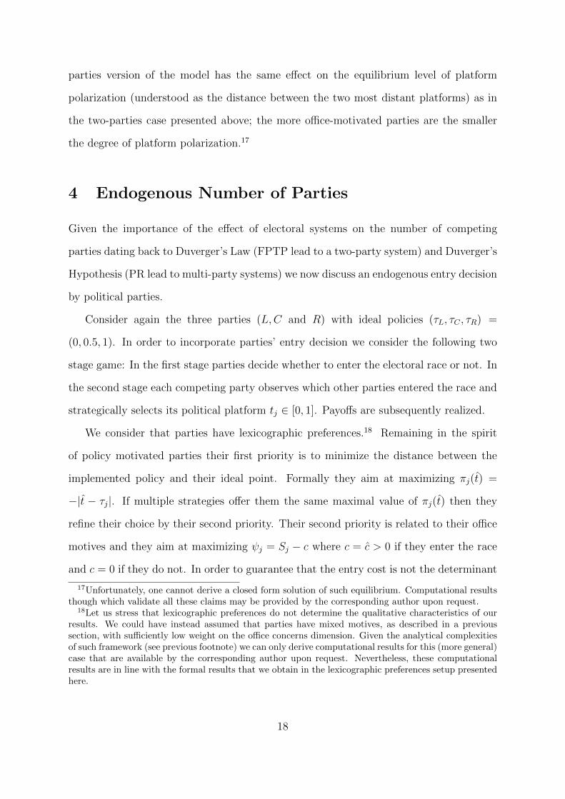
12As the familiar reader with the literature on contests may have already observed, the weights de-termined through this specific functional form are identical to the seminal contest success functionintroduced by Tullock (1980, pg. 97-112). Remember though that since we assume that n � 1, andas depicted in figure 1, the weight function is convex for values smaller than one-half, and concave forvalues larger than one-half. Hence, in the electoral contest winning the elections makes a difference. Theelectoral system gives disproportional weight to the party that obtains the majority of the votes. Up towhat extent the winner is favored is determined by the disproportionality parameter n.

8

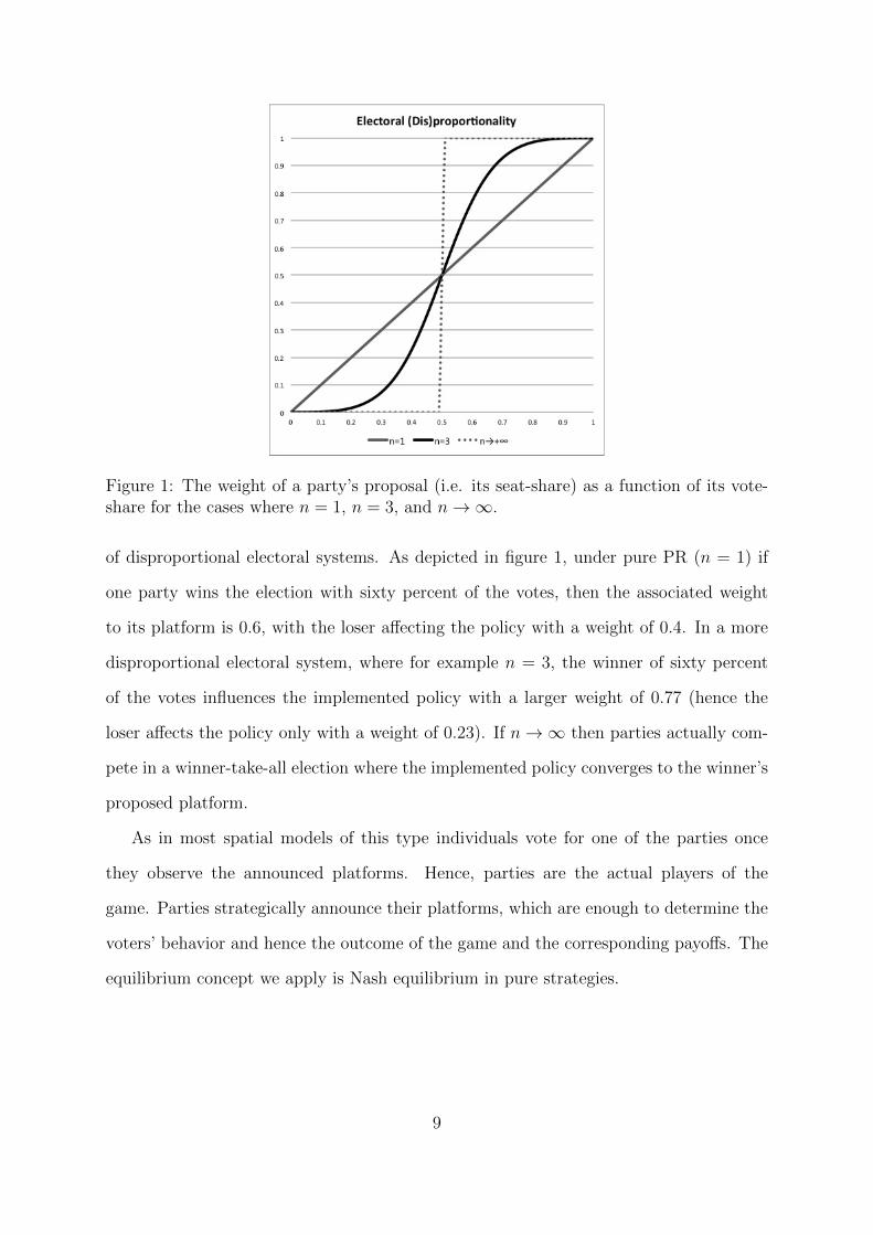
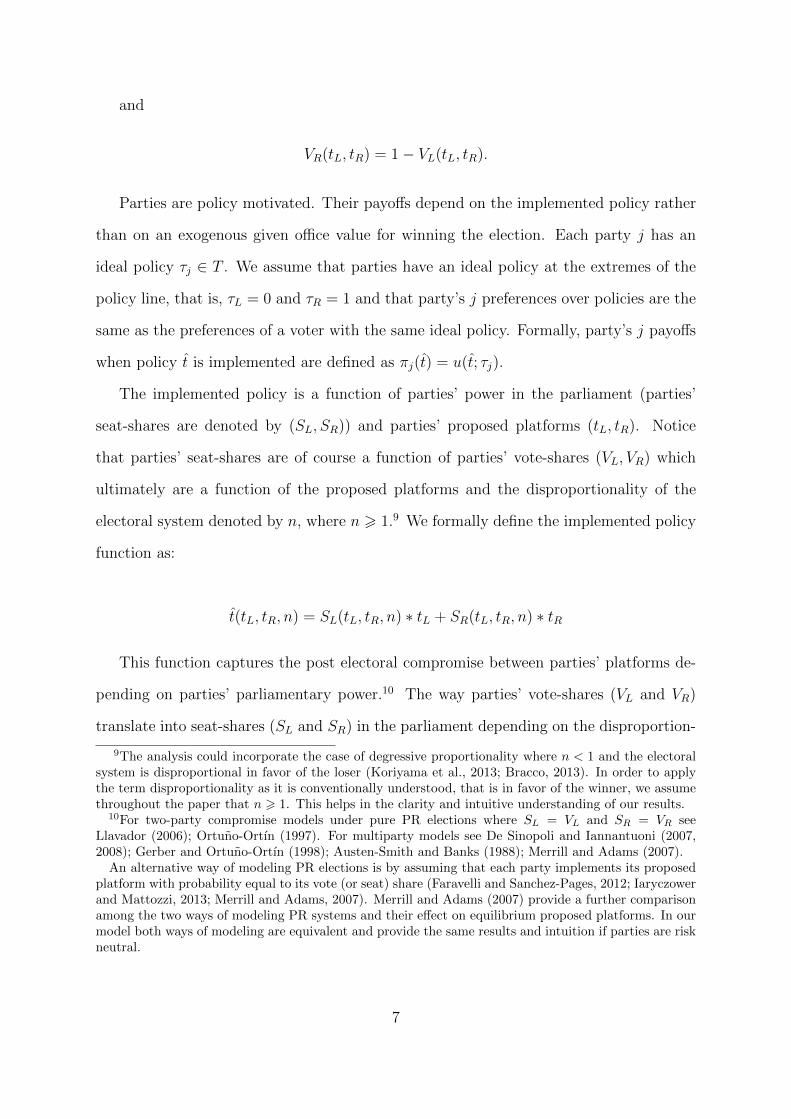
Figure 1: The weight of a party’s proposal (i.e. its seat-share) as a function of its vote-share for the cases where n = 1, n = 3, and n → ∞.

of disproportional electoral systems. As depicted in figure 1, under pure PR (n = 1) if

one party wins the election with sixty percent of the votes, then the associated weight

to its platform is 0.6, with the loser affecting the policy with a weight of 0.4. In a more

disproportional electoral system, where for example n = 3, the winner of sixty percent

of the votes influences the implemented policy with a larger weight of 0.77 (hence the

loser affects the policy only with a weight of 0.23). If n → ∞ then parties actually com-

pete in a winner-take-all election where the implemented policy converges to the winner’s

proposed platform.

As in most spatial models of this type individuals vote for one of the parties once

they observe the announced platforms. Hence, parties are the actual players of the

game. Parties strategically announce their platforms, which are enough to determine the

voters’ behavior and hence the outcome of the game and the corresponding payoffs. The

equilibrium concept we apply is Nash equilibrium in pure strategies.

9

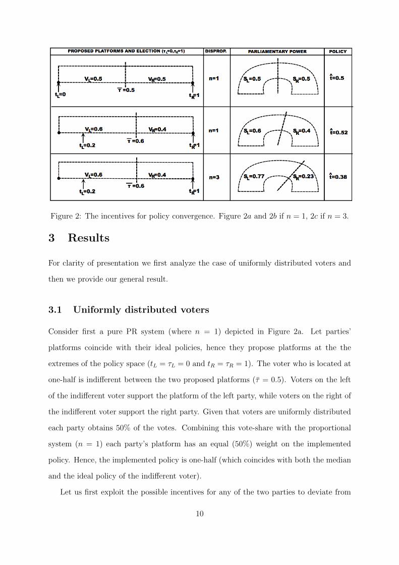
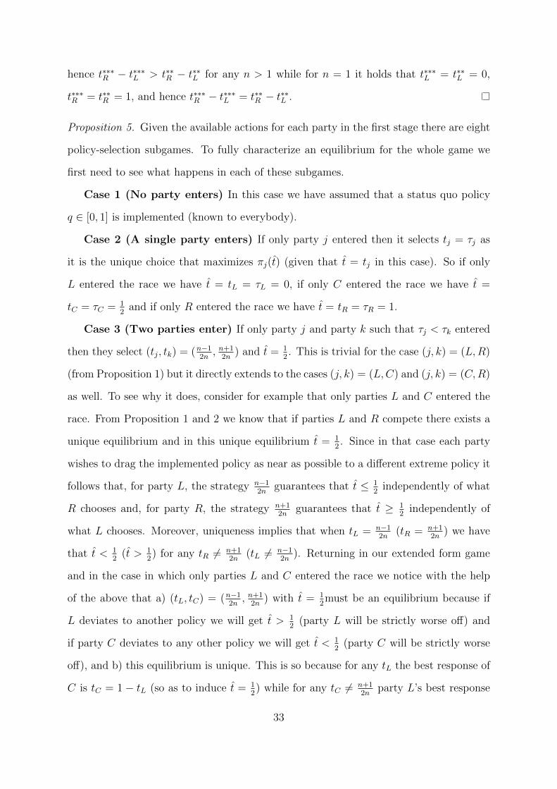
Figure 2: The incentives for policy convergence. Figure 2a and 2b if n = 1, 2c if n = 3.

3 Results

For clarity of presentation we first analyze the case of uniformly distributed voters and

then we provide our general result.

3.1 Uniformly distributed voters

Consider first a pure PR system (where n = 1) depicted in Figure 2a. Let parties’

platforms coincide with their ideal policies, hence they propose platforms at the the

extremes of the policy space (tL = τL = 0 and tR = τR = 1). The voter who is located at

one-half is indifferent between the two proposed platforms (τ = 0.5). Voters on the left

of the indifferent voter support the platform of the left party, while voters on the right of

the indifferent voter support the right party. Given that voters are uniformly distributed

each party obtains 50% of the votes. Combining this vote-share with the proportional

system (n = 1) each party’s platform has an equal (50%) weight on the implemented

policy. Hence, the implemented policy is one-half (which coincides with both the median

and the ideal policy of the indifferent voter).

Let us first exploit the possible incentives for any of the two parties to deviate from

10

this strategy and converge towards the median (Figure 2b). Let for example party L

announce platform tL = 0.2. Now the indifferent voter moves further to the right (now

τ = 0.6). Hence, party L obtains 60% of the votes while party R obtains 40% of the votes.

When the implemented policy is determined party L now has a larger weight than before

(now 60% compared to 50%), but at the same time proposes a policy further from its

ideal point (tL = 0.2 compared to tL = 0). Therefore the implemented policy is t = 0.52

and hence party L has no incentives to deviate from its initial strategy since by doing so

the implemented policy moves further from its ideal point and is worse off.

Consider now that the electoral system is more disproportional, hence it favors the

winner of the election (let for example n = 3) as depicted in Figure 2c. As before,

if party L announces platform 0.2 rather than zero, it obtains 60% of the vote-share.

Because of the disproportionality such vote-share translates to a disproportionally high

weight of 77% on its proposed platform. In contrast to the case when n = 1 such weight

now compensates the loss because of proposing a moderate platform. It turns out that

the implemented policy is 0.38. Hence, party L has incentives to converge towards the

median since it brings the implemented policy closer to its ideal point.

The general mechanism which provides incentives to parties to propose less differenti-

ated platforms when the degree of disproportionality of the electoral rule increases must

have been made clear by now. Analyzing a uniform distribution of voters, though, does

not only formally prove the negative direction of this relationship but further guarantees

a closed form solution regarding parties’ equilibrium strategies. That is, it enhances our

understanding on quantitative aspects of the relationship between platform polarization

and electoral rule disproportionality other than its direction.

Proposition 1. Let τi ∼ U [0, 1]. Then: (i) There exists a unique equilibrium (t∗∗L , t∗∗R ) =

(n−12n ,

n+12n ) (ii) The distance between t

∗∗R and t

∗∗L is decreasing in n (iii) t = τ = 0.5.

The unique equilibrium (t∗∗L , t∗∗R ) of two party competition for different values of elec-

toral disproportionality n ∈ [1, 20] and a graphical interpretation of proposition 1 is

11

Figure 3: The effect of electoral disproportionality n ∈ [1, 20] on proposed platforms fortwo (t∗∗L , t

∗∗R ) and three-party competition (t∗∗∗L , t

∗∗∗R , t

∗∗∗C ) as characterized in propositions

1 and 4.

depicted in figure 3. If n = 1 (i.e. no distortions are present) both parties’ platforms

coincide with their ideal policies, hence they stick at the the extremes of the policy space

(t∗∗L = τL = 0 and t∗∗R = τR = 1). It is easy to calculate that the unique equilibrium when

n = 3 is (t∗∗L , t∗∗R ) = (1/3, 2/3). In the extreme case of a winner-take-all election (n → ∞)

where the winner can perfectly implement his platform we obtain the standard result of

full convergence to the median.

3.2 The General Result

The following result generalizes the case of a uniform distribution to any cumulative

distribution function F .

Proposition 2. Let m denote the median of any c.d.f. F . Then: (i) There exists a

unique equilibrium (t∗L(n), t∗R(n)) where t

∗L(n) < t

∗R(n) (ii) If for some n0 we have that

0 < t∗L(n0) < t

∗R(n0) < 1 then t(n0) = τ(n0) = m and for every n1 and n2 such that

n0 < n1 < n2 we have |t∗L(n1) − t∗R(n1)| > |t∗L(n2) − t

∗R(n2)| (iii) t

∗L(n) → t

∗R(n) when

12

n → ∞ (iv) If m = 0.5 then t∗L = 1− t

∗R.

For any degree of disproportionality there exists a unique equilibrium where the leftist

party proposes a policy at the left of the median and the rightist party proposes a policy

at the right of the median voter. In equilibrium the implemented policy coincides with

the median voter’s ideal point while both parties propose platforms that diverge from

the median by the same distance. Despite our analysis allowing any possible distribution

of voters’ ideal points, as we show, parties propose platforms that are symmetric with

respect to the median no matter how skewed the distribution is. The asymmetry in terms

of the distribution is of course reflected in parties’ payoffs.

From a comparative perspective, as the disproportionality of the electoral system

increases parties have incentives to moderate their policies and converge towards the me-

dian. Full convergence to the median is predicted in the case of winner-take-all elections

(n → ∞). The intuition behind parties’ incentives to moderate or not their platforms

is similar to the case of uniformly distributed voters. If the disproportionality increases

parties have incentives to deviate from the initial equilibrium and moderate their propos-

als aiming at a higher vote-share since the latter further translates to a disproportionally

higher weight in the implemented policy. Such higher weight may well compensate the

losses entailed because of proposing more moderate platforms. Consequently, in the

unique equilibrium, parties’ platforms tend to differentiate less as the disproportionality

of the electoral system increases.

3.3 Further Results

We now discuss three possible directions of enrichening our model that provide an intu-

ition in line with our main result and the centrifugal incentives present in proportional

systems.

13

3.4 Office motivated parties

So far we have considered purely policy motivated parties. Remember that party’s j

payoffs when policy t was implemented were defined as πj(t) = u(t; τj). Let us modify

that payoff specification by considering that parties have mixed motives and also care

for holding office. Formally we define party’s j payoffs as πj = αSj − (1 − α)|τj − t|

where α ∈ [0, 1) denotes the importance parties attach to the appropriation of office

rents.13 We do not allow parties to be purely office motivated (that is α = 1) since this

would always yield the standard Downsian prediction of full convergence to the median

no matter the electoral disproportionality (Downs, 1957). When parties are both office

and policy motivated the following result holds:

Proposition 3. Let τi ∼ U [0, 1]. Then: (i) There exists a unique equilibrium (tαL, tαR) =

(min{ n−1+α2n(1−α) ,

12},max{1

2 ,n+1−α(2n+1)

2n(1−α) }) (ii) The distance between tαR and t

αL is decreasing

in n (iii) The distance between tαR and t

αL is decreasing in α (iv) t = τ = 0.5.

As before in the unique equilibrium parties parties’ proposed platforms are symmetric

around the median. If parties are purely policy motivated (α = 0) the result replicates

the one of proposition 1. If parties have mixed motives and are partially interested in

extracting office rents then office rents act as a centripetal force. Proportional electoral

systems on the contrary still provide centrifugal incentives. If office motives are not

strong enough then parties in equilibrium propose diverged platforms that depend on the

proportionality of the electoral system. If office motives are strong enough such that they

compensate the centrifugal incentives provided by the electoral system then both parties

propose the same platform (tαL = tαR = 0.5 if α > 1/(n+ 1)).

Notice that despite the presence of office motives proportional electoral systems still

provides the aforementioned centrifugal incentives. As n decreases parties differentiate

13Notice that we implicitly assume that the value for holding office is one. Moreover, while in ourgeneral results we used a general utility function u(t; τj) here we assume that parties have a linearutility function when they value the implemented policy. Different utility specifications (for examplea quadratic utility function) or different positive values for office would pronounce one of the motivesversus the other. Intuition would remain the same no matter our assumptions. Office motives act as acentripetal force while proportionality remains an active centrifugal force.

14

more. The centrifugal incentives provided by the electoral system are however less intense

than in proposition 1 since the presence of office motives always acts as a balancing

centripetal force (that is tαL ≥ t∗∗L and t

αR ≤ t

∗∗R ).

3.5 Non-extreme parties

The main result of our paper as presented in proposition 2 incorporates a large degree

of generality since it does not impose any restrictions on the distribution of voters’ ideal

points. As we have shown, no matter how asymmetric the society is and whether one party

is favored compared to its opponent, both parties have incentives to converge towards the

median as the disproportionality of the electoral system increases. This general result

can be generalized regarding parties’ ideal policies.

It can be shown that our general result (Proposition 2) holds in the case of non-

extreme parties (0 < τL < m < τR < 1) and voters that are uniformly distributed.

For more general distributions some further structure is required. In particular, if we

define party’s L weight on the implemented policy as a function SJ where SJ(x, n) =

F (x)n

F (x)n+(1−F (x))n and assume that SJ is log-concave in x then if for some n0 we have that

0 < t∗L(n0) < t

∗R(n0) < 1 then for every n1 and n2 such that n0 < n1 < n2 we can show

that there exists a unique equilibrium where |t∗L(n1)− t∗R(n1)| > |t∗L(n2)− t

∗R(n2)|. Hence

we can show that the more disproportional the electoral system is the less polarized the

equilibrium.14

14Notice that the assumption of log-concavity is usually imposed on the distribution of voters’ idealpoints F (for example in Llavador 2006; Ortuno-Ortın 1997). However, here we require that the weightfunction SJ is log-concave. Intuitively this means that as a party proposes a more moderate platformthen its seat-share and hence its weight in the implemented policy increases at a decreasing rate. In orderto relate the log-concavity of SJ with the primitives of the model it can be shown that SJ is log-concavefor a large family of F ’s. A general example guaranteeing the log-concavity of SJ is when voters aredistributed according to any unimodal beta distribution (that is τi ∼ Beta(α,β) with α ≥ 1,β ≥ 1).

15

3.6 The Three Parties Case

We now consider the case of a three-party electoral race (a leftist, a centrist and a rightist

party).15 It is straightforward that the complexity of the analysis increases several orders

in magnitude when we increase the cardinality of the set of players from two to three. For

example, the game is no longer strictly competitive as when only two-parties compete

and, hence, the equilibrium characterization cannot follow from a standard combination

of the popular properties that strictly competitive games have (see proof of Proposition

2). Hence, to guarantee tractability some further assumptions are in order. We consider

that a) the ideal policy of the centrist party is at one-half (that is τC = 0.5) and the leftist

and the rightist party are modeled as in the two-party scenario analyzed above (τL = 0

and τR = 1) and b) an equilibrium in this case is a pure-strategy Nash equilibrium such

that the distribution of policy proposals is symmetric about the center of the policy space.

Since now three parties compete in the election each party’s seat-share is given by the

following expression (Theil, 1969; Taagepera, 1986):

SJ =V

nJ

VnL + V

nC + V

nR

and therefore the implemented policy function for the three-party model is accordingly

defined as:

t(tL, tC , tR, n) =VL(tL, tR)n

VL(tL, tR)n + VC(tL, tR)n + VR(tL, tR)n∗ tL

+VC(tL, tR)n

VL(tL, tR)n + VC(tL, tR)n + VR(tL, tR)n∗ tC

+VR(tL, tR)n

VL(tL, tR)n + VC(tL, tR)n + VR(tL, tR)n∗ tR

The following result holds:16

15The result trivially extends to k parties where two parties have ideal policies at the two extremes(that is at 0 and 1) and k − 2 parties have an ideal policy at 0.5.

16Without providing a formal definition of voters’ strategies it is necessary to mention that each voteri supports party j that proposes the closest platform to his ideal policy. If a voter is indifferent betweentwo or even three platforms then he randomizes his vote.

16

Proposition 4. Let τi ∼ U [0, 1]. Then: (i) There exists a unique equilibrium (t∗∗∗L , t∗∗∗C , t

∗∗∗R ) =

( n−12(n+1) , 0.5,

n+32(n+1)) (ii) The distance between t

∗∗∗R and t

∗∗∗L is decreasing in n (iii) t = τ =

0.5.

As we observe the centrist party proposes a platform equal to its ideal policy (t∗∗∗C =

τC = 0.5). The two other parties differentiate and propose more extreme platforms.

The extent to what parties differentiate depends on the level of disproportionality (see

figure 3 depicting the proposed platforms (t∗∗∗L , t∗∗∗R ) for different values of electoral dis-

proportionality n ∈ [1, 20]). The more proportional the electoral system is, the higher are

the centrifugal forces, and hence polarization increases. As it was the case for our gen-

eral result and two-party competition electoral proportionality acts as a centrifugal force.

Clearly, if parties compete in a winner-take-all election (n → ∞) then the standard result

of convergence to the median applies (that is (t∗∗∗L , t∗∗∗C , t

∗∗∗R ) = (0.5, 0.5, 0.5)). Note that

the qualitative implications of the above proposition directly extend to a general class of

distributions (at least for the class of log-concave distributions) and are not restricted to

the uniform case.

Corollary 1. Polarization in a three-party election is larger than in a two-party election

(t∗∗∗R − t∗∗∗L ≥ t

∗∗R − t

∗∗L with the equality holding for n = 1)

Notice that the centrifugal force identified in the proportionality of the electoral sys-

tem is now amplified as the number of competing parties increases. Comparing the

proposed platforms by the leftist and rightist party we observe that in the unique equi-

librium of the three-party election they polarize more than in the two-party election (for

any n > 1 it holds that t∗∗∗L < t

∗∗L and that t

∗∗∗R > t

∗∗R ). The presence of a third party

makes competition for centrist voters tougher and hence parties have less incentives to

moderate their policies in the hunt of more votes. This comparative result can be visual-

ized in Figure 3 where for every value n polarization is higher three-party than two-party

competition (t∗∗∗R − t∗∗∗L ≥ t

∗∗R − t

∗∗L ).

Finally, note that inclusion of minor-to-moderate office-holding concerns in this three-

17

parties version of the model has the same effect on the equilibrium level of platform

polarization (understood as the distance between the two most distant platforms) as in

the two-parties case presented above; the more office-motivated parties are the smaller

the degree of platform polarization.17

4 Endogenous Number of Parties

Given the importance of the effect of electoral systems on the number of competing

parties dating back to Duverger’s Law (FPTP lead to a two-party system) and Duverger’s

Hypothesis (PR lead to multi-party systems) we now discuss an endogenous entry decision

by political parties.

Consider again the three parties (L,C and R) with ideal policies (τL, τC , τR) =

(0, 0.5, 1). In order to incorporate parties’ entry decision we consider the following two

stage game: In the first stage parties decide whether to enter the electoral race or not. In

the second stage each competing party observes which other parties entered the race and

strategically selects its political platform tj ∈ [0, 1]. Payoffs are subsequently realized.

We consider that parties have lexicographic preferences.18 Remaining in the spirit

of policy motivated parties their first priority is to minimize the distance between the

implemented policy and their ideal point. Formally they aim at maximizing πj(t) =

−|t − τj|. If multiple strategies offer them the same maximal value of πj(t) then they

refine their choice by their second priority. Their second priority is related to their office

motives and they aim at maximizing ψj = Sj − c where c = c > 0 if they enter the race

and c = 0 if they do not. In order to guarantee that the entry cost is not the determinant

17Unfortunately, one cannot derive a closed form solution of such equilibrium. Computational resultsthough which validate all these claims may be provided by the corresponding author upon request.

18Let us stress that lexicographic preferences do not determine the qualitative characteristics of ourresults. We could have instead assumed that parties have mixed motives, as described in a previoussection, with sufficiently low weight on the office concerns dimension. Given the analytical complexitiesof such framework (see previous footnote) we can only derive computational results for this (more general)case that are available by the corresponding author upon request. Nevertheless, these computationalresults are in line with the formal results that we obtain in the lexicographic preferences setup presentedhere.

18

of the qualitative features of the equilibrium we assume that c < 0.25.

Regarding the implemented policy we assume that a) if only party j enters then its

platform is implemented (t(tj) = tj), b) if two parties enter then the implemented policy

is determined as in the benchmark two-party case and c) if all three parties enter then

the implemented policy is determined as in the three-party case presented in the previous

section. For simplicity we assume that if no party enters a status quo policy q ∈ [0, 1] is

implemented and that this status quo policy is known to all parties (this assumption can

be relaxed). We can now state the main proposition regarding parties’ equilibrium entry

and platform decisions.

Proposition 5. If τi ∼ U [0, 1] then there exists a unique subgame perfect equilibrium and

a unique n > 0 such that: (i) for n < n all three parties enter and their platform choices

are (t∗∗∗L , t∗∗∗C , t

∗∗∗R ) = ( n−1

2(n+1) , 0.5,n+3

2(n+1)) (ii) for n > n only parties L and R enter and

their platform choices are (t∗∗L , t∗∗R ) = (n−1

2n ,n+12n ).

The above result is depicted in figure 4. For a given entry cost if the electoral system

is sufficiently proportional (low values of n) all three parties have incentives to pay the

entry cost and compete in the election. In the case of three-party competition the centrist

party sticks to its ideal policy (t∗∗∗C = 0.5) while the two other parties announce platforms

that diverge symmetrically around that point. Since three parties have entered the race

their policy choices are identical to the ones described in proposition 4 and the policy

implemented coincides with the one of the median (t = 0.5).

As the electoral system becomes more disproportional the two extreme parties con-

verge towards the center and suppress the seat-share of the centrist party. From a point

on (when n > n) the seat-share of the centrist party is suppressed sufficiently such that

the centrist party is better off by not paying the entry cost. Notice that no matter whether

two or three parties compete the implemented policy coincides with the ideal point of

the centrist party and hence the latter competes only to maximize its office benefits (its

second priority). Hence for sufficiently disproportional electoral systems only two parties

remain active in the political arena.

19

Figure 4: The effect of electoral disproportionality n ∈ [1, 10] on the number of competingparties and proposed platforms as characterized in proposition 5. In the graph we depictthe case of c = 0.22 which implies that n = 2.5.

As clearly depicted in the graph notice that as the disproportionality increases tL

and tR converge smoothly towards the center up to the point when n = n. This is

the direct effect of electoral disproportionality on polarization described in Proposition

4. Once disproportionality is sufficiently high (n = n) we observe an indirect effect of

disproportionality on polarization that is attributed to the the depicted jump provoked by

the decision of the centrist party not to enter the political race. Hence we observe that the

direct effect is further amplified by the indirect effect and the fact that disproportionality

affects the number of competing parties.

5 Empirical Analysis

We formulate the two following institutional hypotheses in order to test the main theo-

retical predictions of our model: Disproportionality has a direct effect on platform polar-

ization and an indirect one through its effect on the number of competing parties.

20

(H1) Electoral System Hypothesis (Propositions 1 and 2): Platform polarization (dis-

tance between parties’s platforms) is decreasing in the disproportionality of the electoral

rule (n).

(H2) The Number of Parties Hypothesis (Corollary 1 to Proposition 4): Platform

polarization is increasing in the number of parties participating in the election.

Both hypotheses have been explored by a number of related studies in the past yield-

ing mixed empirical findings. While most approaches fail to garner enough support for

H1 (e.g., Budge and McDonald 2006; Ezrow 2008; Dalton 2008; Curini and Hino 2012)

few of them provide some (conditional) evidence in favor of either H1 (e.g., Calvo and

Hellwig 2011; Dow 2011) or H2 (Andrews and Money, 2009).19 Let us mention that most

existing studies utilized small and unbalanced data sets (see Table A.1) and were therefore

restricted to only exploit cross-country variation thus making level comparisons across

countries. On top of it, by including very few observations for many of these countries

(in some instances only one) they are, in fact, estimating those level effects using just a

single observation for each country. That is, they just provide a snapshot of polarization

at a given point in time (which incidentally is not the same across different countries)

and compare it. This additional limitation does not allow to disentangle between vari-

ation in polarization that is related to electoral rules and variation that is due to other

sources (e.g. time or country specific shocks). Therefore, by considering an enlarged and

balanced sample, that includes at least ten observations for each country, our work is

an improvement on both fronts: not only we introduce some within country variation

in the electoral rule disproportionality (though admittedly limited) but we also improve

significantly the cross-country comparison, thus obtaining a more accurate picture of the

19For a complete comparative presentation of the empirical literature, hypotheses tested and theirfindings see Table A1 in the Appendix. Curini and Hino (2012) find support for the voters’ hypothesesand two additional institutional hypotheses: the cabinet-parties conditional hypothesis and the electoralspill-over hypothesis. Including the relevant variables in the institutional controls we do not find asignificant effect of spill-overs while some specifications provide partial support regarding the cabinet-parties conditional hypothesis. In addition to their full model, Curini and Hino (2012) also test a simplerversion that includes only H1 and H2 and which is directly comparable to our model in columns 1 and 2 inTable A4. The fact that we find find a statistically significant effect of disproportionality on polarizationwhile they do not cannot therefore be attributed to the exclusion of the hypotheses mentioned above.

21

effects of interest instead of a snapshot.

5.1 Data Description and Measurement

We construct a balanced panel that combines electoral, political, institutional, socioeco-

nomic, and demographic data for more than 300 elections from 23 OECD countries during

the period from 1960 to 2006 (on average 13 elections in each country). We describe our

data and the main variables thereafter and provide summary statistics in Table A2 of the

Appendix.

The Dependent Variable: Platform Polarization

Our dependent variable, platform polarization, is constructed using data from the

Volkens et al. (2012) Comparative Manifesto Project (CMP) dataset compiled by the

Wissenschaftszentrum Berlin fur Sozialforschung (WZB). The latter records the ideolog-

ical position of the platforms proposed by hundreds of political parties since 1946 (in line

with our theoretical model we consider a unidimensional policy space in a 0 − 10 scale

where zero stands for extreme left and ten for extreme right).20 In order to maintain

consistency with recent literature we follow Dalton (2008) and formally define the index

of platform polarization (IPi) in election i as:21

IPi =

�����

j

Vj

�Pji − Pi

5

�2

where Pi denotes the weighted mean of parties’ position on the left-right dimension (each

party j is weighted by its vote-share Vj) and Pji is the ideological position of party j in

20Technically, the CMP provides parties’ positions on a −100 to 100 scale. We perform an affine,monotonic, order preserving transformation of the index by adding 100 to each party’s position then,dividing the sum by 20. Other studies that use the CMP to measure platform polarization are: Budgeand McDonald (2006); Ezrow (2008); Andrews and Money (2009).

21Curini and Hino (2012) also use the Dalton index while Ezrow (2008); Dow (2011) use a very closeanalogue that incorporates all parties’ positions weighted by their vote-shares. In Table A3 of theAppendix we replicate our estimates using another measure of polarization (as in Budge and McDonald2006; Andrews and Money 2009): the distance between the two most extreme parties. The use of suchindex not only serves as a robustness check but further allows for an one-to-one correspondence betweenour theoretical predictions and the empirical estimation. Our results are robust to different measures ofpolarization.

22

election i (0-10 scale), normalized by the mid-point ideology position (5).

The index takes value zero when all parties converge to a single position and ten when

parties are equally split between the two extreme positions. Two important properties

of this index is that it is relatively independent of the number of competing parties and

that weighting for the electoral size of each party implies that a large party at one of the

extremes implies greater polarization than a marginal party in the same position (Curini

and Hino, 2012).

The Main Explanatory Variables: Electoral Rule Disproportionality and

the Number of Competing Parties

Our key explanatory variable is the measure of electoral rule (dis)proportionality. By

combining data from two different sources (Armingeon et al. 2012 (CPDS I) and the

Carey 2012 archive) we use two alternative measures, one continuous and one binary,

that provide qualitatively identical results. In models sub-indexed with an a we consider

a binary variable that takes value zero whenever the FPTP rule with single-member

districts applies and one otherwise. In models sub-indexed with b we control for the

mean magnitude of electoral districts: larger magnitude reduces the effective threshold

required for a party to occupy a parliamentary seat, hence, making the electoral system

more proportional (Taagepera, 1986).

The use of the two alternative measures increases the robustness of our findings and

allows us to address any concerns related to limited within country variation of our

independent variable.22 On one hand, the binary variable records only a radical change

from a FPTP rule to a more proportional one and vice versa. Since such radical changes

are not frequent this is a slow-moving institutional variable.23 On the other hand, the

continuous version of our independent variable is more sensitive to changes in the electoral

rule and allows for some within country variation. Both specifications provide results that

22Incidentally, limited within country variation can also ease to some extend, albeit not completelyeradicating, any potential concerns over endogeneity and reverse causality.

23In most countries in the sample such radical change occurred at most once (save for Greece, Italyand New Zealand) while in some countries no such change ever occurred (e.g. USA, UK, and theNetherlands).

23

are equally robust, statistically significant and identical in the direction of the effect.

We test the number of competing parties hypothesis (H2) by using two different mea-

sures of the explanatory variable. The first one is the Effective Number of Parties (ENP)

index.24 The second is the actual number of parties participating in the election. Since

our findings in all specifications do not vary significantly when we substitute the ENP

with the actual number of parties we present all our results controlling for the ENP in

order to guarantee consistency with the literature. The results when we control for the

actual number of parties are presented only for Model 1 (See Table 1).25

5.2 Empirical Estimation

Model 1 jointly tests our two primary institutional hypotheses: the impact of the electoral

rule (dis)proportionality (H1) and the number of competing parties (H2) in determining

polarization. Since empirical evidence (e.g. Gallagher 1991) and theoretical literature

(e.g. Duverger 1954) suggest that electoral rules may also affect polarization through the

structure of the party-system (e.g. number of parties) we test our first two hypotheses

jointly (e.g. Cox 1990) in order to prevent a biased estimation.26 Model 1 serves as our

benchmark since most of the literature tests these two hypotheses (e.g. Dalton 2008;

Ezrow 2008; Andrews and Money 2009; Dow 2011; Calvo and Hellwig 2011). Formally,

we estimate the following model:

IPit = α0+β1(PROPORTIONALITY )it+β2(NUMBEROFPARTIES )it+λt+γi+�it (1)

According to H1, we expect β1 to be positive as more proportional rules should lead

to more polarization. From H2, we also expect β2 to be positive. To fully exploit the

advantages of a large balanced panel we introduce country (γi) and time (λt) dummies

24Laakso and Taagepera (1979) define the effective number of political parties as 1/�

j(Vj)2.25Similar to Andrews and Money (2009) we also control for the Log ENP (see Table A3 in the Ap-

pendix).26Also note that our result in Proposition 5 suggests a close link between the proportionality of the

electoral rule and the number of competing parties.

24

(fixed effects).

In Model 2 we control for a set of other relevant institutional variables: coalition

habits dummy, number of parties participating in government/cabinet and their inter-

action, type of political regime (presidentialism vs. parliamentarianism), degree of in-

stitutional constraints, years of consolidated democracy, a dummy variable indicating

government change, the ideological distance between incumbent and past government.

Model 3 further controls for some socioeconomic variables: unemployment rate, GDP

growth rate, government spending (as % of GDP), Gini coefficient of inequality. Finally,

in tables A.3 and A.4 we estimate Models 4, 5 and 6 that incorporate some additional

robustness checks using alternative measures of our dependent and independent variables

as well as a model with random effects (Model 6).

Results

Table 1 contains the combined results of the econometric estimations that provide

strong support for our main hypothesis (H1) at any conventional level of significance and

irrespective of how the (dis)proportionality of the electoral system is measured. In all

specifications, we find that more proportional electoral rules are associated with increased

levels of polarization. This finding is robust to various alterations of the model, including

different ways of measuring both the dependent and independent variables (as presented

in the Appendix) and the inclusion of more control variables (Models 2 and 3). Hence,

our empirical analysis verifies the main theoretical prediction of the model on the effect

of electoral rule (dis)proportionality on polarization.

This result contrasts with existing literature where electoral institutions have no im-

pact on polarization (e.g. Dow 2001; Budge and McDonald 2006; Dalton 2008; Ezrow

2008; Andrews and Money 2009; Curini and Hino 2012) and reinforces recent work by

Dow (2011) and Calvo and Hellwig (2011) who find some conditional support for the

Electoral System (H1) hypothesis. According to our results not only is the coefficient β1

positive (as predicted) and statistically significant, but it is also large in magnitude. Our

estimates can associate a switch from a FPTP to a PR rule (electoral system becomes

25

Table 1: The Impact of Electoral Rule Disproportionality on Platform Polarization in OECD Democracies (from 1960-2007)

Dependent Variable Dalton Index of Party-System (Platform) Polarization

Explanatory Variables

Model 1.a

PR rule

Model 1.b

District Magnitude

Model 2.a

PR rule

Model 2.b

District Magnitude

Model 3.a

PR rule

Model 3.b

District Magnitude

(1) (2) (3) (4) (5) (6) (7) (8) H1 Electoral Rule Dummy (PR = 1) 1.659 1.743 -.- -.- 1.326 -.- 1.263 -.- (0.181)*** (0.193)*** (0.268)*** (0.283)*** H1 Log Avg. Electoral District Magnitude -.- -.- 0.264 0.280 -.- 0.195 -.- 0.222 (0.071)*** (0.074)*** (0.094)** (0.068)*** H2 Effective Number of Parties (ENP) 0.009 -.- 0.033 -.- -0.012 0.002 -0.136 -0.113 (0.064) (0.079) (0.151) (0.154) (0.181) (0.181) H2 Actual Number of Parties -.- -0.040 -.- -0.033 -.- -.- -.- -.- (0.041) (0.046) Country Dummies? ! ! ! ! ! ! ! ! Year Dummies? ! ! ! ! ! ! ! ! Other Institutional Controls? No No No No Yes Yes Yes Yes Economic Controls? No No No No No No Yes Yes R^2 0.39 0.39 0.41 0.41 0.43 0.41 0.63 0.62 N 307 307 255 255 237 237 123 123

* p < 0.10; ** p < 0.05; *** p < 0.01 Robust standard errors clustered at the country level reported in parentheses. Country and year dummies (fixed effects) are included in all specifications. Other institutional controls include: a (dummy) variable indicating strong coalition habbits and its interaction with ENP, the number of parties participating in government/cabinet, the type of political regime (presidentialism/parliamentarianism), the degree of institutional constraints (a categorical variable taking values from 0 - 6), years of consolidated democracy, a (dummy) variable indicating government change and the ideological distance between incumbent and past government. Economic controls include: unemployment rate (in %), GDP growth rate (in %), government spending (as % of GDP), Gini coefficient of inequality. Model 3 has less observations due to missing economic data from 1960-1980. Models 1.b and 2.b also have some missing values for the average electoral district size. In all models the dependent variable (polarization) is constructed as in Dalton (2008).

more proportional) with a two standard deviations increase in polarization. In other

words, a one-standard-deviation increase in the average district magnitude is associated

with a half standard deviation increase in polarization.

On the other hand, the number of parties hypothesis (H2) is confirmed under few

specifications since the number of political parties does not appear to have a consistent

significant effect on polarization regardless of the measurement technique (neither the

ENP nor the actual number of parties).27 One plausible explanation, in line with our

theoretical predictions (Proposition 5), is that any potential effect that the number of

parties may have on polarization operates via the electoral system itself (e.g., Duverger

1954). To better see this point, we have estimated the correlation between the number

of parties (actual and effective) and the electoral rule (dis)proportionality (using both

the binary and the continuous variable). In all cases the correlation coefficient is of the

27The models where H2 is validated are presented in Table A3 of the Appendix is Model 4 where forrobustness we control for the log of ENP following Andrews and Money (2009) and in Table A4 in twoof the specifications (columns 2 and 8) where where we use the random effects estimator.

26

magnitude of 0.50 and is also statistically significant at any conventional level.

Overall, our empirical results yield robust support for the main prediction of the

theoretical model (H1) on the effect of electoral rule (dis)proportionality on platform

convergence. The combination of our theoretical and empirical findings suggest that far

from being “the dog that did not bark” (Ezrow 2008) the (dis)proportionality of the

electoral rule is the most important institutional determinant of platform polarization.

Discussion

Our empirical analysis complements previous literature (summarized in Table A1

in the Appendix) in two main aspects. First, by combining different sources of data

(CPDS I, CMP and the Carey archive) we construct a balanced panel of 23 advanced

democracies (OECD states) with a large number of electoral observations (more than

300) over a 50-year-long time frame. Second, our study simultaneously considers: a)

both continuous and categorical measures of the electoral rule (dis)proportionality; b)

two different measures of platform polarization (one that uses information on vote-share

distribution and one that does not); c) alternative measures for the number of competing

parties; and d) both country and year fixed effects.

Our analysis addresses a common concern associated with studies that, given data

limitations, use unbalanced panels that often contain few observations for a large num-

ber of countries and are forced to group together a set of diverse countries that share

different and divergent institutional history and traditions (e.g., Curini and Hino 2012;

Dow 2011).28 Such unbalanced panels may result not only to observable differences in

electoral institutions but also to important unobservable, or difficult to measure at best,

differences among various other institutional features.

Regarding our model specification itself, while country and year dummies (fixed ef-

fects) help us account both for idiosyncratic country-specific characteristics (country dum-

28Examples of studies with a limited set of observations are the ones using the CSES mass surveys(e.g., Dalton 2008; Dow 2011; Curini and Hino 2012) and also studies by Budge and McDonald (2006);Ezrow (2008) despite the use of the CMP data because they aggregate their data across countries orthey have a limited time frame.

27

mies) and also for year specific effects, their inclusion is not the reason why our results

differ from previous findings. This can be seen in Table A.4 where we compare the fixed

effects model estimates with those of a model that omits country and year dummies (as

for example in Curini and Hino 2012) and a random effects one.29 While different in

magnitude, the estimates regarding H1 obtained under all three specifications are quali-

tatively identical, equally statistically significant, and on the same direction. Therefore,

we attribute this significant difference with previous findings to our better data.

6 Concluding Remarks

Our work has implications on the design of electoral institutions as it surfaces an in-

teresting trade-off between the need for more democratic pluralism and wider political

representation (served by more proportional rules) and political stability and modera-

tion (served more by majoritarian rules). Hence, the choice of one class of rules over

the other is not as straightforward as one might think and a lot seems to depend on

individual party-system characteristics and the attributes of each polity. Moreover, as-

sumptions regarding voters’ behavior, other than the ones explored in this paper, should

be carefully explored in future studies. Possibility of abstention and of strategic voting

are just two out of the many examples of such alternative behavioral elements that could

be incorporated in the analysis.

As far as abstention is concerned, a simple extension of the model suggests that our

results are robust to allowing voters to abstain. If for instance one considers that the

society is normally distributed around the median and that alienated voters whose ideal

29Since we have argued that we have limited within country variation on our binary electoral rule vari-able (in some countries there is at most one change while in others none) one might question whether theinclusion of country fixed effects in our model is appropriate. The reason is that under such specificationthe fixed effects estimated coefficient on the electoral rule disproportionality is in fact driven only bythose few countries that had frequent “radical” changes in the electoral rule and therefor a random ef-fects estimator may seem more appropriate. Since the results we obtain using a random effects estimatorare qualitatively identical, albeit smaller in magnitude, equally statistically significant and in the samedirection with both the fixed effects and the simple model estimates, we believe that there is no furtherreason to worry. In fact the use of both fixed and random effects allows us to frame the real impact ofelectoral rule disproportionality by estimating upper (FE) and lower (RE) bounds for the effect.

28

policies are “sufficiently” away from the parties’ platforms do not vote for the party that

proposes a platform closer to their ideal policies but rather abstain then an increase in

the electoral disproportionality would still reduce the level of polarization.

Finally, in our analysis voters are expressive and support the party that proposes the

platform closest to their ideal point. But what if some voters behaves strategically? Intu-

ition suggests that the presence of strategic voters provides further centrifugal incentives

to political parties (Llavador, 2006; De Sinopoli and Iannantuoni, 2007). As before, a sim-

ple extension of the model shows that our main result would persist. That is, the degree

of polarization would be higher when compared to the case of a completely non-strategic

electorate but the direction of the effect of the degree of electoral rule disproportionality

on the level of platform polarization would not be affected. But what if the electoral

system itself endogenously determines the share of voters that behave strategically? To

gain a complete picture of how disproportionality affects polarization such alternative

channels, through which these two variables could possibly interact, should be further

investigated.

29

7 Appendix

7.1 Proofs

Proposition 1. Follows proposition 2.

Proposition 2. We prove our general result in four steps.

Step 1 (Player j has a unique best response for every t−j) We notice that for

any tR ∈ [0, 1] we have that t(tL, tR, n) = tR whenever tL = tR and that t(tL, tR, n) > tR

whenever tL > tR. Since, the utility of L, u(t, 0), is strictly decreasing in t it follows that

the best response of party L to R playing tR, bL(tR), can never be such that bL(tR) > tR.

In specific, if tR = 0 this implies that bL(tR) = tR = 0. When tR > 0 we observe that

t(tL, tR, n) = tR whenever tL = tR and that t(tL, tR, n) < tR whenever tL = 0. Since, the

utility of L, u(t, 0), is strictly decreasing in t it follows that the best response of party L

to R playing tR, bL(tR), can never be such that bL(tR) ≥ tR whenever tR > 0.

Moreover, we know that for tL < tR:

t(tL, tR, n) =VL(tL,tR)n

VL(tL,tR)n+VR(tL,tR)n × tL + VR(tL,tR)n

VL(tL,tR)n+VR(tL,tR)n × tR =

=F (

tL+tR2 )n

F (tL+tR

2 )n+[1−F (tL+tR

2 )]n× tL +

[1−F (tL+tR

2 )]n

F (tL+tR

2 )n+[1−F (tL+tR

2 )]n× tR.

Observe that:

∂u(t,0)∂tL

= ∂u(t,0)∂ t

× ∂ t(tL,tR,n)∂tL

.

Since we always have that ∂u(t,0)∂ t

< 0 it must be the case that sign[∂u(t,0)∂tL] = −sign[∂ t(tL,tR,n)

∂tL].

Now, notice that:

F (tL+tR

2 )n

F (tL+tR

2 )n+[1−F (tL+tR

2 )]n× tL

is strictly increasing in tL ∈ [0, tR) and that:

[1−F (tL+tR

2 )]n

F (tL+tR

2 )n+[1−F (tL+tR

2 )]n× tR

is strictly decreasing in tL ∈ [0, tR).

That is, t(tL, tR, n) is strictly quasi-convex in tL ∈ [0, tR) and therefore u(t, 0) is

strictly quasi-concave in tL ∈ [0, tR).

All the above suggest that for any tR ∈ [0, 1] there exist a unique bL(tR). Due to the

symmetry of our game it is straighforward that bR(tL) is also single-valued.

30

Step 2 (Existence of an equilibrium) Following the arguments of Ortuno-Ortın

(1997) and given the single-valuedness of bL(tR) and bR(tL) we can define B : [0, 1]2 →

[0, 1]2 as B(tL, tR) = (bR(tL), bL(tR)). Notice that due to the continuity of F and u and

Berge’s maximum theorem it directly follows that B is continuous. That is, Brower’s

fixed point theorem applies in our case and guarantees existence of an equilibrium point.

Step 3 (Uniqueness of the equilibrium) Notice that sign[∂u(t,0)∂ t

] = −sign[∂u(t,1)∂ t

].

That is, our game is strictly competitive (Aumann, 1961; Friedman, 1983) and has the

same properties as a zero-sum game. Assume that the game admits two equilibria (t∗L, t∗R)

and (t∗L, t∗R) such that either t∗L �= t

∗L or t∗R �= t

∗R or both. Assume without loss of generality

that at least t∗L �= t∗L holds. Since our game is strictly competitive it directly follows that

(t∗L, t∗R) and (t∗L, t

∗R) are also equilibria of the game. This implies bL(t∗R) = t

∗L and that

bL(t∗R) = t∗L. Since t

∗L �= t

∗L this contradicts the fact that bL(t∗R) is always single-valued.

Therefore, the game must admit a unique equilibrium point.

Step 4 (Characterization of the equilibrium) Notice that t∗L < t

∗R because

in any other case at least one of the two parties is strictly better off by switching to

her ideal policy. If 0 < t∗L < t

∗R < 1 (interior equilibrium) it must be the case that

∂u(t,0)∂t∗L

= ∂u(t,0)∂t∗R

= 0. Algebraic manipulations of these two equilibrium conditions lead to

a) F (t∗L+t∗R

2 ) = 12 and therefore to

t∗L+t∗R2 = m and to b) 1

nf(m) = t∗R − t

∗L; the degree of

platform polarization is decreasing in n. Notice that when n → ∞ it holds that t∗R → t∗L

and when m = 0.5 then t∗R + t

∗L = 1 and hence t

∗L = 1− t

∗R.

Proposition 1. Given that for the uniform distribution it holds that f(m) = 1 and from

Step 4 of Proposition 1 that 1nf(m) = t

∗∗R − t

∗∗L we can rewrite the latter as 1

n = t∗∗R − t

∗∗L .

Moreover since for the uniform distribution m = 0.5 and hence from step 4 we know that

t∗∗L = 1− t

∗∗R we obtain that 1

n = 2t∗∗R − 1 which implies that t∗∗R = n+12n and therefore that

t∗∗L = n−1

2n .

Proposition 3. We first check that the presented strategy profile is indeed a Nash equilib-

rium of the game. If we define tαR = 1− t

αL = max{1

2 ,n+1−α(2n+1)

2n(1−α) } one can algebraically

31

verify that πL(tαL, tαR) > πL(tL, tαR) for every tL �= t

αL; (tαL, t

αR) is a Nash equilibrium.

As far as uniqueness is concerned, we observe that πL(tL, tR) + πR(tL, tR) = 1 for any

(tL, tR) ∈ [0, 1]2. Hence, our game is a constant-sum game. This implies that if another

equilibrium (tαL, tαR) exists it should be the case that (tαL, t

αR) is a Nash equilibrium too.

But, as we argued, πL(tαL, tαR) > πL(tL, tαR) for every tL �= t

αL. Hence πL(tαL, t

αR) > πL(tαL, t

αR)

and, thus, (tαL, tαR) cannot be an equilibrium.

Proposition 4. Let us first describe some properties of an equilibrium and then proceed to

the existence proof. Since we are interested in strategy profiles which induce a symmetric

distribution of policy proposals about the center of the policy space, in equilibrium it

must be the case that t∗∗∗J < t

∗∗∗Q = 0.5 < t

∗∗∗Z = 1 − t

∗∗∗J for J,Q, Z ∈ {L,C,R} and

t(t∗∗∗L , t∗∗∗C , t

∗∗∗R , n) = 1

2 .30 Notice that if Q = L (Q = R) then party L (R) has incentives

to deviate away from 0.5 and bring the implemented policy closer to its ideal policy.

Hence in equilibrium it must be that Q = C, that is, that t∗∗∗C = 0.5. Moreover notice

that if J = R and Z = L then party L (R) has incentives to deviate (to offer the same

platform as party R (L) for example) and bring the implemented policy closer to its ideal

policy. Hence, in equilibrium it should be the case that J = L, Q = C and Z = R. That

is, it should hold that t∗∗∗L < t∗∗∗C = 0.5 < t

∗∗∗R = 1− t

∗∗∗L .

But could such a strategy profile be a Nash equilibrium of the game? Since in every

such strategy profile we have that t(tL, tC , tR, n) = 12 then party C has no incentives

to deviate. Moreover, observe that the utility of party L (R) is strictly decreasing (in-

creasing) in t(tL, tC , tR, n). One can algebraically verify that a) t( n−12(n+1) , 0.5, tR, n) <

12

for every tR �= n+32(n+1) , b) and t(tL, 0.5,

n+32(n+1) , n) >

12 for every tL �= n−1

2(n+1) and that c)

t( n−12(n+1) , 0.5,

n+32(n+1)) = 1

2 . Hence, there exists a unique equilibrium and it is such that

(t∗∗∗L , t∗∗∗C , t

∗∗∗R ) = ( n−1

2(n+1) , 0.5,n+3

2(n+1)).

Corollary 1. From proposition 1 we have that (t∗∗L , t∗∗R ) = (n−1

2n ,n+12n ). From proposition

4 we have that (t∗∗∗L , t∗∗∗R ) = ( n−1

2(n+1) ,n+3

2(n+1)). It is clear that t∗∗∗L < t

∗∗L , t∗∗∗R > t

∗∗R and

30The case t∗∗∗L = t∗∗∗C = t∗∗∗R = 0.5 is trivially ruled out as party L (R) has clear incentives to deviateand bring the implemented policy nearer to its ideal policy.

32

hence t∗∗∗R − t

∗∗∗L > t

∗∗R − t

∗∗L for any n > 1 while for n = 1 it holds that t

∗∗∗L = t

∗∗L = 0,

t∗∗∗R = t

∗∗R = 1, and hence t

∗∗∗R − t

∗∗∗L = t

∗∗R − t

∗∗L .

Proposition 5. Given the available actions for each party in the first stage there are eight

policy-selection subgames. To fully characterize an equilibrium for the whole game we

first need to see what happens in each of these subgames.

Case 1 (No party enters) In this case we have assumed that a status quo policy

q ∈ [0, 1] is implemented (known to everybody).

Case 2 (A single party enters) If only party j entered then it selects tj = τj as

it is the unique choice that maximizes πj(t) (given that t = tj in this case). So if only

L entered the race we have t = tL = τL = 0, if only C entered the race we have t =

tC = τC = 12 and if only R entered the race we have t = tR = τR = 1.

Case 3 (Two parties enter) If only party j and party k such that τj < τk entered

then they select (tj, tk) = (n−12n ,

n+12n ) and t = 1

2 . This is trivial for the case (j, k) = (L,R)

(from Proposition 1) but it directly extends to the cases (j, k) = (L,C) and (j, k) = (C,R)

as well. To see why it does, consider for example that only parties L and C entered the

race. From Proposition 1 and 2 we know that if parties L and R compete there exists a

unique equilibrium and in this unique equilibrium t = 12 . Since in that case each party

wishes to drag the implemented policy as near as possible to a different extreme policy it

follows that, for party L, the strategy n−12n guarantees that t ≤ 1

2 independently of what

R chooses and, for party R, the strategy n+12n guarantees that t ≥ 1

2 independently of

what L chooses. Moreover, uniqueness implies that when tL = n−12n (tR = n+1

2n ) we have

that t < 12 (t > 1

2) for any tR �= n+12n (tL �= n−1

2n ). Returning in our extended form game

and in the case in which only parties L and C entered the race we notice with the help

of the above that a) (tL, tC) = (n−12n ,

n+12n ) with t = 1

2must be an equilibrium because if

L deviates to another policy we will get t >12 (party L will be strictly worse off) and

if party C deviates to any other policy we will get t < 12 (party C will be strictly worse

off), and b) this equilibrium is unique. This is so because for any tL the best response of

C is tC = 1 − tL (so as to induce t = 12) while for any tC �= n+1

2n party L’s best response

33

induces t < 12 . All these obviously hold (in the reverse way) for the (j, k) = (C,R) case

as well.

Case 4 (All three parties enter) If all three parties enter then we are in the case

of Proposition 4 and (tL, tC , tR) = ( n−12(n+1) , 0.5,

n+32(n+1)) and t = 1

2 .

So each policy selection subgame has essentially a unique equilibrium. This makes

identification of a subgame perfect equilibrium (SPE) tractable.

First, we argue that in a SPE at least two parties should enter. If no party is expected

to enter then the implemented policy will be q ∈ [0, 1]. In that case a party j with τj �= q

is strictly better off by entering and, thus, implementing her ideal policy. If only one

extreme party is expected to enter and implement its ideal policy then the other extreme

party, for example, is better off by entering too and, thus, moving the implemented policy

to 12 . If only the centrist party is expected to enter and implement its ideal policy (12)

then an extreme party has incentives to enter. By entering the extreme party will not

affect the implemented policy (we argued in case 3 that if the centrist runs against an

extremist then the implemented policy will be 12) but will enjoy an increase in the second

element of its lexicographic preferences, ψj. This is so because if the extremist j does not

enter and only the centrist party runs, then ψj = 0 (because Sj = 0 and c = 0) but if it

runs against the centrist it will enjoy ψj = 0 (because Sj =12 and c <

12).

Second, we will argue that if a SPE in which all three parties enter exists then gener-

ically no SPE exists in which only two parties enter. This is straightforward for the

following reason. If a SPE in which all three parties enter exists then this implies that

if a party expects that only the two other parties will run it also strictly prefers to run

(apart from cases of measure zero in which for some party/ies Sj = c in the equilibrium

of the three party subgame); entering does not affect implemented policy but increases

the value of ψj.

Third, we notice that in the equilibrium of the three party subgame ∂SC∂n < 0. This

implies that in the equilibrium of the three party subgame ∂SL∂n = ∂SR

∂n > 0.

By a careful composition of the above we arrive to result. When n = 1 we know

34

that in the equilibrium of the three party subgame SL = SR = 14 and SC = 1

2 . Since

c <14 it follows that for n = 1 all three parties entering and selecting (t∗∗∗L , t

∗∗∗C , t

∗∗∗R ) =

( n−12(n+1) , 0.5,

n+32(n+1)) is the a SPE of the game. This is so because if a party j deviated to not

entering it would not affect the implemented policy but it would get a strictly lower ψj.

Moreover, by our first and second argument it becomes evident that this SPE is unique.

By increasing n our third observation dictates that the SPE in which all three parties

enter is still the unique one as long as SC > c. Since ∂SC∂n < 0 and for n → ∞ we have that

SC → 0 there should exist some n > 0 such that for every n < n we have SC > c and for

every n > n we have SC < c. For n < n as stated above we have a unique SPE and in this

equilibrium all three parties enter. For n > n the unique SPE is such that only parties L

and R enter and their platform choices are (t∗∗L , t∗∗R ) = (n−1

2n ,n+12n ). Existence is established

by the following argument. If only parties L and R are expected to run then C is strictly

better off by not running. Its decision to enter does not affect the implemented policy

but if it does not run it gets ψC = 0 while if it runs it gets ψC < 0. Party L (R) is strictly

better off by running because if it does not the other extremist party will run alone and

will thus implement its ideal policy, while if it runs the implemented policy will be 12 .

Uniqueness is guaranteed by the facts that a) an equilibrium with three parties entering

is not feasible (as party C is strictly better off by staying out when the other two are

expected to run) and b) if another SPE exists it should be such that only parties L and

C (R and C) run. If party R expects that parties L and C will run then it is strictly

better off by running. Its entry decision will not affect the implemented policy but it

will increase its ψR from zero (in the case of no entry) to something strictly positive (in

the case of entry). This is so because in the equilibrium of the three party subgame a)

ψR > 0 for n = 1 and b) ∂ψR

∂n = ∂SR∂n > 0.

35

7.2 Summary Statistics and Result Tables

Table A.1: Summary of empirical findings on Party-system Polarization (adapted from Curini & Hino, 2012)

Paper Type of data Sample size

Time-period

Measure of Polarization Hypotheses Tested Conclusion

Dow, 2001

National mass surveys

4 countries

1988-1994

Two-dimensional space using parties' and voters'

positions

Electoral System

Not confirmed

Budge & McDonald, 2006

Comparative Manifesto Project (CMP)

17 countries

1945-1998

Unidimensional space using the distance between the two most extreme parties

Electoral System

Not confirmed

Dalton, 2008

Comparative Studies of Electoral Systems

(CSES) mass surveys

35 countries (most with 1 observation)

1996-2006

Unidimensional space using all parties' positions

weighted by vote-shares

Electoral System & Party-system size

Both not confirmed

Ezrow, 2008

Expert-surveys and CMP for parties'

positions/Eurobarometer for voters' positions

18 countries

1980-1990

Unidimensional space using all parties' positions

weighted by vote-shares and voter distribution

Electoral System & Party-system size

Both not confirmed

Andrews & Money, 2009

Comparative Manifesto

Project (CMP)

20 countries

1945-1998

2-dimensional space using the distance between the two most extreme parties

Electoral System & Party-system size

First not confirmed Second confirmed

Dow, 2011

CSES surveys

30 countries (most with 1 observation)

1996-2006

Same as in Ezrow 2008

Electoral System & Party-system size

First confirmed Second not confirmed

Calvo & Hellwig, 2011

CSES-2 surveys

13 countries

2001-2006

Condtional Logit estimates based on Adams, Merrill & Grofman (2005) predictions

Electoral System

Hypothesis Conditionally

confirmed Curini and Hino, 2012

CSES-3surveys

36 countries (some with more than 1 observation

1996-2006

Same as in Dalton 2008

Electoral System Party-system size

Coalition Habits & Voters' Distribution

First and second not confirmed. Third and

fourth confirmed

This paper

CMP, Carey-Hix Data

Archive

Balanced panel of 23

OECD states

1960-2007

Same as in Dalton 2008; repeat estimates using

Budge & McDonald 2006

Electoral System Party-system size

First confirmed. Second conditionally

confirmed

Sheet1

Page 1

Table A2: Summary Statistics of Key Explanatory Variables

Variable Obs. Mean Std. Dev. Min Max

Electoral Rule Dummy (PR =1) 307 0.80 0.40 0 1

Type of Political Regime (Presidential = 1) 264 0.29 0.45 0 1

Coalition Habbits Dummy (Coal. Govt.= 1) 302 0.55 0.50 0 1

Polarization (Dalton Index 0-10) 307 1.70 0.79 0.23 5.14

Polarization (Distance between extremes) 307 2.43 1.10 0.34 6.55

Electoral District Magnitude (Average) 268 16.9 34.4 1 150

(Log of) Avg. Electoral District Magnitude 268 1.71 1.44 0 5.01

Years of consolidated Democracy 267 49.9 20.7 1 87

Effective Number of Electoral Parties 307 4.1 1.5 2.0 10.3

Actual Number of Parties 307 5.6 2.2 1 12

No of Parties participating in Gov't/Cabinet 264 2.0 1.3 1 6

Degree of Institutional Constraints (0-6) 307 2.2 1.5 0 5

GDP growth rate (in %) 307 3.5 2.6 -7.3 14.6

Government spending (% of GDP) 155 20.2 5.3 10.3 34.9

Unemployment rate (in %) 307 5.3 3.9 0.0 22.8

Gini coefficient of inequality 264 33.4 6.2 20.5 61.0Note: Data reported at electoral not calendar year. Source: Comparative Political Studies Data Set 1, Carey-Hix DataArchive and the Manifesto Project Database. Period of observation: 1960 – 2007 for 23 OECD States.

36

Table A.3: The Impact of Electoral Rule Disproportionality on Platform Polarization in OECD Democracies (from 1960-2007)

Dependent Variable Platform Distance between the Two Most Extreme Parties

Explanatory Variables

Model 4.a

PR rule

Model 4.b

Electoral District Magnitude

Model 5.a

PR rule

Model 5.b

District Magnitude

(1) (2) (3) (4) (5) (6) (7) (8) H1 Electoral Rule Dummy (PR= 1) 2.291 2.182 2.238 -.- -.- -.- 2.124 -.- (0.243)*** (0.252)*** (0.243)*** (0.339)*** H1 Log Avg. Electoral District Magnitude -.- -.- -.- 0.401 0.371 0.401 -.- 0.344 (0.093)*** (0.094)*** (0.091)*** (0.112)*** H2 Effective Number of Parties (ENP) 0.112 -.- -.- 0.169 -.- -.- 0.118 0.134 (0.113) (0.129) (0.152) (0.154) H2 Log ENP -.- 0.790 -.- -.- 1.104 -.- -.- -.- (0.464)* (0.526)** H2 Actual Number of Parties -.- -.- 0.062 -.- -.- 0.066 -.- -.- (0.052) (0.058) Country Dummies? ! ! ! ! ! ! ! ! Year Dummies? ! ! ! ! ! ! ! ! Other Institutional Controls? No No No No No No Yes Yes Economic Controls? No No No No No No No No R^2 0.55 0.56 0.55 0.61 0.61 0.60 0.64 0.63 N 307 307 307 255 255 255 237 237

* p < 0.10; ** p < 0.05; *** p < 0.01 Robust standard errors clustered at the country level reported in parentheses. Country and year dummies (fixed effects) are included in all specifications. In Model 5, other institutional controls include: a (dummy) variable indicating strong coalition habbits and its interaction with ENP, the number of parties participating in government/cabinet, the type of political regime (presidentialism/parliamentarianism), the degree of institutional constraints (a categorical variable taking values from 0 - 6), years of consolidated democracy, a (dummy) variable indicating government change and the ideological distance between incumbent and past government. Model 4.b has some missing values for the average electoral district size. In Model 4, the dependent variable (polarization) is measured as the distance between the two most extreme parties (as in Budge and McDonald 2006 and Andrews and Money 2009). In Models 4.a and 4.b we employ alternative measures for the size of the party-system in order to control for H2. In Models 5.a and 5.b we only use the Effective Number of Parties (ENP) for consistency with Table 1.

Table A.4: The Impact of Electoral Rule Disproportionality on Platform Polarization in OECD Countries (1960-2007): Random vs. Fixed Effects

Dependent Variable Dalton Index of Party-System (Platform) Polarization

Explanatory Variables

Curini & Hino (2012)

Baseline Model

Models 1.a & 2.a

Fixed Effects

Model 6.a

Random Effects

(1) (2) (3) (4) (5) (6) (7) (8) H1 Electoral Rule Dummy (PR = 1) 0.377 0.375 1.423 1.659 1.326 0.590 0.471 0.561 (0.148)** (0.183)** (0.066)*** (0.181)*** (0.268)*** (0.230)*** (0.168)*** (0.196)*** H2 Effective Number of Parties (ENP) 0.020 0.084 -0.038 0.009 -0.012 -0.010 0.028 0.142 (0.069) (0.049)* (0.056) (0.064) (0.151) (0.052) (0.073) (0.076)* Country Dummies? X X ! ! ! X X X Year Dummies? X X X ! ! X ! ! Random Effects? X X X X X ! ! ! Other Institutional Controls? No Yes No No Yes No No Yes R^2 0.04 0.15 0.28 0.39 0.42 0.08 0.27 0.68 N 307 237 307 307 237 307 307 237

* p < 0.10; ** p < 0.05; *** p < 0.01 Robust standard errors clustered at the country level reported in parentheses. The first two columns replicate the estimates using the Curini and Hino (2012) econometric specification on our data set. In columns 3 to 5 (Models 1.a and 2.a) country dummies (country fixed effects) are included in all specifications. In addition, in columns 4 and 5 we also include year dummies (year fixed effects). In columns 6 to 8 (Model 6.a) we estimate a random effects model (in columns 7 and 8 we also include year dummies). Other institutional controls include: a (dummy) variable indicating strong coalition habbits and its interaction with ENP, the number of parties participating in government/cabinet, the type of political regime (presidentialism/parliamentarianism), the degree of institutional constraints (a categorical variable taking values from 0 - 6), years of consolidated democracy, a (dummy) variable indicating government change and the ideological distance between incumbent and past government. Columns 2, 5 and 8 have less observations due to missing data for some institutional variables for the period from 1960 to 1980. In all models the dependent variable (platform polarization) is constructed as in Dalton (2008).

37

References

Adams, J., S. Merrill III, and B. Grofman (2005): A unified theory of partycompetition: A cross-national analysis integrating spatial and behavioral factors, Cam-bridge University Press.

Andrews, J. and J. Money (2009): “The spatial structure of party competition:Party dispersion within a finite policy space,” British Journal of Political Science, 39,805–824.

Armingeon, K., P. Potolidis, M. Gerber, and P. Leimgruber (2012): Com-parative Political Data Set I(CPDS I), 1960-2010, Bern: Institute of Political Science,University of Bern.

Aumann, R. (1961): “Almost strictly competitive games,” Journal of the Society forIndustrial & Applied Mathematics, 9, 544–550.

Austen-Smith, D. (2000): “Redistributing income under proportional representation,”Journal of Political Economy, 108, 1235–1269.

Austen-Smith, D. and J. Banks (1988): “Elections, coalitions, and legislative out-comes,” American Political Science Review, 82, 405–422.

Besley, T. and I. Preston (2007): “Electoral bias and policy choice: theory andevidence,” Quarterly Journal of Economics, 122, 1473–1510.

Bracco, E. (2013): “Optimal districting with endogenous party platforms,” Journal ofPublic Economics, 104, 1 – 13.

Budge, I. and M. McDonald (2006): “Choices Parties Define Policy Alternatives inRepresentative Elections, 17 Countries 1945–1998,” Party Politics, 12, 451–466.

Calvert, R. (1985): “Robustness of the multidimensional voting model: Candidatemotivations, uncertainty, and convergence,” American Journal of Political Science, 29,69–95.

Calvo, E. and T. Hellwig (2011): “Centripetal and centrifugal incentives underdifferent electoral systems,” American Journal of Political Science, 55, 27–41.

Carey, J. M. (2012): Carey data archive.

Coate, S. and B. Knight (2007): “Socially optimal districting: a theoretical andempirical exploration,” Quarterly Journal of Economics, 122, 1409–1471.

Cox, G. (1990): “Centripetal and centrifugal incentives in electoral systems,” AmericanJournal of Political Science, 34, 903–935.

Curini, L. and A. Hino (2012): “Missing links in party-system polarization: Howinstitutions and voters matter,” Journal of Politics, forthcoming.

38

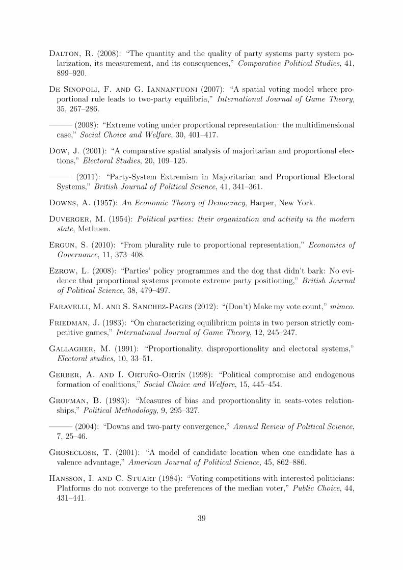
Dalton, R. (2008): “The quantity and the quality of party systems party system po-larization, its measurement, and its consequences,” Comparative Political Studies, 41,899–920.

De Sinopoli, F. and G. Iannantuoni (2007): “A spatial voting model where pro-portional rule leads to two-party equilibria,” International Journal of Game Theory,35, 267–286.

——— (2008): “Extreme voting under proportional representation: the multidimensionalcase,” Social Choice and Welfare, 30, 401–417.

Dow, J. (2001): “A comparative spatial analysis of majoritarian and proportional elec-tions,” Electoral Studies, 20, 109–125.

——— (2011): “Party-System Extremism in Majoritarian and Proportional ElectoralSystems,” British Journal of Political Science, 41, 341–361.

Downs, A. (1957): An Economic Theory of Democracy, Harper, New York.

Duverger, M. (1954): Political parties: their organization and activity in the modernstate, Methuen.

Ergun, S. (2010): “From plurality rule to proportional representation,” Economics ofGovernance, 11, 373–408.

Ezrow, L. (2008): “Parties’ policy programmes and the dog that didn’t bark: No evi-dence that proportional systems promote extreme party positioning,” British Journalof Political Science, 38, 479–497.

Faravelli, M. and S. Sanchez-Pages (2012): “(Don’t) Make my vote count,” mimeo.

Friedman, J. (1983): “On characterizing equilibrium points in two person strictly com-petitive games,” International Journal of Game Theory, 12, 245–247.

Gallagher, M. (1991): “Proportionality, disproportionality and electoral systems,”Electoral studies, 10, 33–51.

Gerber, A. and I. Ortuno-Ortın (1998): “Political compromise and endogenousformation of coalitions,” Social Choice and Welfare, 15, 445–454.

Grofman, B. (1983): “Measures of bias and proportionality in seats-votes relation-ships,” Political Methodology, 9, 295–327.

——— (2004): “Downs and two-party convergence,” Annual Review of Political Science,7, 25–46.

Groseclose, T. (2001): “A model of candidate location when one candidate has avalence advantage,” American Journal of Political Science, 45, 862–886.

Hansson, I. and C. Stuart (1984): “Voting competitions with interested politicians:Platforms do not converge to the preferences of the median voter,” Public Choice, 44,431–441.

39

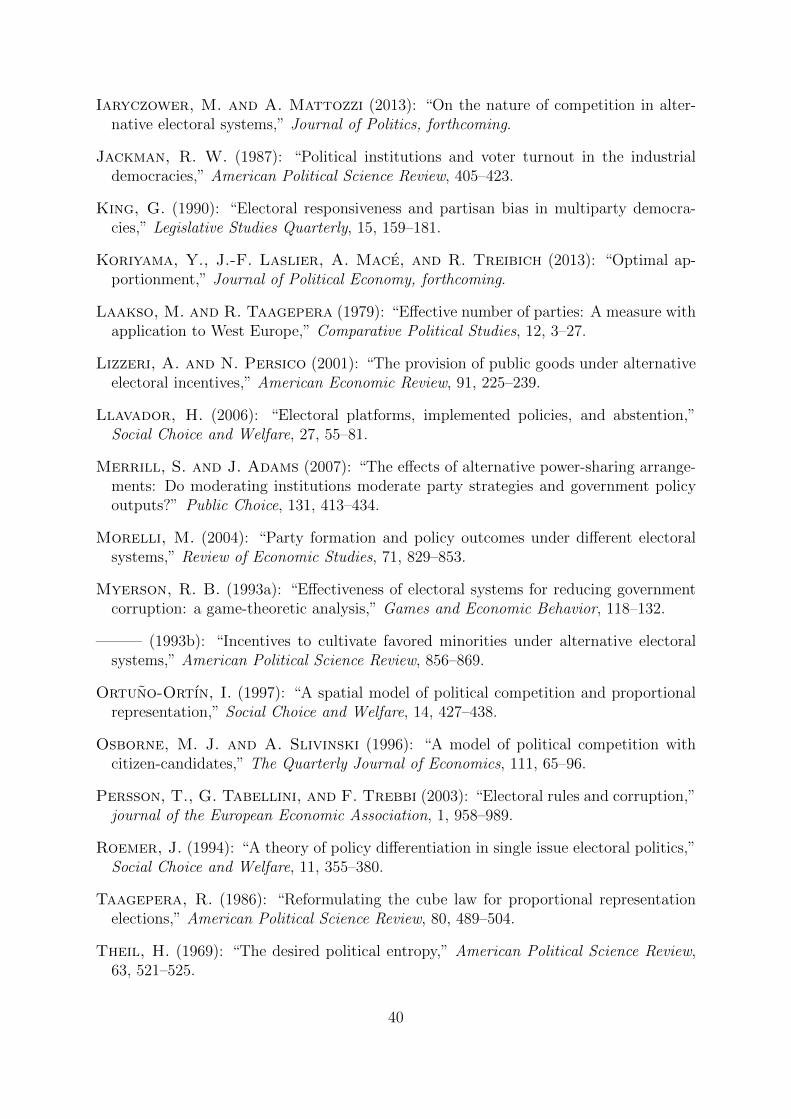
Iaryczower, M. and A. Mattozzi (2013): “On the nature of competition in alter-native electoral systems,” Journal of Politics, forthcoming.

Jackman, R. W. (1987): “Political institutions and voter turnout in the industrialdemocracies,” American Political Science Review, 405–423.

King, G. (1990): “Electoral responsiveness and partisan bias in multiparty democra-cies,” Legislative Studies Quarterly, 15, 159–181.

Koriyama, Y., J.-F. Laslier, A. Mace, and R. Treibich (2013): “Optimal ap-portionment,” Journal of Political Economy, forthcoming.

Laakso, M. and R. Taagepera (1979): “Effective number of parties: A measure withapplication to West Europe,” Comparative Political Studies, 12, 3–27.

Lizzeri, A. and N. Persico (2001): “The provision of public goods under alternativeelectoral incentives,” American Economic Review, 91, 225–239.

Llavador, H. (2006): “Electoral platforms, implemented policies, and abstention,”Social Choice and Welfare, 27, 55–81.

Merrill, S. and J. Adams (2007): “The effects of alternative power-sharing arrange-ments: Do moderating institutions moderate party strategies and government policyoutputs?” Public Choice, 131, 413–434.

Morelli, M. (2004): “Party formation and policy outcomes under different electoralsystems,” Review of Economic Studies, 71, 829–853.

Myerson, R. B. (1993a): “Effectiveness of electoral systems for reducing governmentcorruption: a game-theoretic analysis,” Games and Economic Behavior, 118–132.

——— (1993b): “Incentives to cultivate favored minorities under alternative electoralsystems,” American Political Science Review, 856–869.

Ortuno-Ortın, I. (1997): “A spatial model of political competition and proportionalrepresentation,” Social Choice and Welfare, 14, 427–438.

Osborne, M. J. and A. Slivinski (1996): “A model of political competition withcitizen-candidates,” The Quarterly Journal of Economics, 111, 65–96.

Persson, T., G. Tabellini, and F. Trebbi (2003): “Electoral rules and corruption,”journal of the European Economic Association, 1, 958–989.

Roemer, J. (1994): “A theory of policy differentiation in single issue electoral politics,”Social Choice and Welfare, 11, 355–380.

Taagepera, R. (1986): “Reformulating the cube law for proportional representationelections,” American Political Science Review, 80, 489–504.

Theil, H. (1969): “The desired political entropy,” American Political Science Review,63, 521–525.

40

Tullock, G. (1980): Toward a theory of the rent-seeking society, in Buchanan, J.M.and Tollison, R.D. and Tullock, G. (eds.), Texas A & M University Press.

Volkens, A., O. Lacewell, P. Lehmann, S. Regel, H. Schultze,and A. Werner (2012): The manifesto data collection, Manifesto Project(MRG/CMP/MARPOR), Berlin: Wissenschaftszentrum Berlin fur Sozialforschung(WZB).

Wittman, D. (1977): “Candidates with policy preferences: A dynamic model,” Journalof Economic Theory, 14, 180–189.

——— (1983): “Candidate motivation: A synthesis of alternative theories,” AmericanPolitical Science Review, 77, 142–157.

41