Embed Size (px)
Citation preview

ELATION GROUPS OF THE HERMITIAN SURFACE H(3, q2) OVER A
FINITE FIELD OF CHARACTERISTIC 2.
by
Robert L. Rostermundt
B.A., University of Colorado at Boulder, 1993
A thesis submitted to the
University of Colorado at Denver
in partial fulfillment
of the requirements for the degree of
Doctor of Philosophy
Applied Mathematics
2005

This thesis for the Doctor of Philosophy
degree by
Robert L. Rostermundt
has been approved
by
Stan Payne
Bill Cherowitzo
Mike Jacobson
Rich Lundgren
Eric Moorhouse
Date

Rostermundt, Robert L. (Ph.D., Applied Mathematics)
Elation Groups of the Hermitian Surface H(3, q2) Over a Finite Field of Char-acteristic 2.
Thesis directed by Professor Stan Payne
ABSTRACT
Let S = (P,B, I) be a finite generalized quadrangle (GQ) having order
(s, t). Let p be a point of S. A whorl about p is a collineation of S fixing all the
lines through p. An elation about p is a whorl that does not fix any point not
collinear with p, or is the identity. If S has an elation group acting regularly
on the set of points not collinear with p we say that S is an elation generalized
quadrangle (EGQ) with base point p. S. E. Payne posed the following question:
Can there be two non-isomorphic elation groups about the same point p? In this
presentation, we show that there are exactly two (up to isomorphism) elation
groups of the Hermitian surface H(3, q2) over the finite field of characteristic 2.
Moreover, we investigate some possible EGQ’s that may be constructed as a
coset geometry from the new elation groups, and show that the EGQ we con-
struct are isomorphic to the Hermitian surface.
iii

This abstract accurately represents the content of the candidate’s thesis. I
recommend its publication.
SignedStan Payne
iv

DEDICATION
This is dedicated to my parents, whose constant support has helped to make
this thesis a reality.

ACKNOWLEDGMENT
There are many people who have been present with me throughout this
long journey and deserve thanks. I would first like to thank all the members
of my committee for their time and effort. In particular, I thank my advisor
Stan Payne, without whose patience I could have never reached as far as I have.
I can only dream of becoming a mathematician of his stature and reputation.
Furthermore, Bill Cherowitzo has been a constant source of assistance, espe-
cially during the early stages of my career as a graduate student. Here I quote
Newton’s letter to Hooke in 1676, in which he said, “If I have seen further than
others, it is because I was standing on the shoulders of giants.”
I also would like to thank Tim Penttila for selflessly suggesting this problem.
Although we are separated by some distance, he has been extremely supportive
throughout the process.
I also extend my appreciation to the graduate committee for appointing me
a teaching assistant position. This financial support has made a great impact
on my success here at UCD. Moreover, I thank the Warren Bateman Family
for their generous funding of the Lynn Bateman Teaching Fellowship, and the
Lynn Bateman Teaching Award, both of which I was a recipient. These were
established in memory of Lynn Bateman, who had an outstanding reputation
as a teaching assistant in the department.
Finally, over the past six years I have had many friends, both in and out
of the math department, who have encouraged me to push on during the most
difficult times. I can not name them all here, but I would like to thank a few
specific individuals: Marcia Kelly, Jennifer Thurston, Steve Flink, Scott Hace,
Ryan and Natalie McGrath, Christi Day, and also my family, Leo and Elizabeth
and Liz Rostermundt. To all of you, I am in your debt.
Rob Rostermundt
CONTENTS
Figures . . . . . . . . . . . . . . . . . . . . . . . . . . . . . . . . . . . . ix
1. Introduction and Review . . . . . . . . . . . . . . . . . . . . . . . . . 1
1.1 Preface . . . . . . . . . . . . . . . . . . . . . . . . . . . . . . . . . . 1
1.2 Historical Background . . . . . . . . . . . . . . . . . . . . . . . . . 2
1.3 Basic Definitions and Combinatorics . . . . . . . . . . . . . . . . . 3
1.4 Elation Generalized Quadrangles . . . . . . . . . . . . . . . . . . . 5
1.5 Introduction to q-clans . . . . . . . . . . . . . . . . . . . . . . . . . 8
1.6 Some examples of q-clans . . . . . . . . . . . . . . . . . . . . . . . . 10
1.7 q-Clans and Flocks . . . . . . . . . . . . . . . . . . . . . . . . . . . 11
1.8 4-Gonal Families from q-Clans . . . . . . . . . . . . . . . . . . . . . 14
1.9 A Construction of the Hermitian Surface H(3, q2) . . . . . . . . . . 19
1.10 Regularity in H(3, q2) . . . . . . . . . . . . . . . . . . . . . . . . . 20
2. Main Results . . . . . . . . . . . . . . . . . . . . . . . . . . . . . . . 21
2.1 Forming a Sylow2 Subgroup in the Group of Whorls . . . . . . . . . 21
2.2 Elation Groups of H(3, q2) As Subgroups of S2 . . . . . . . . . . . . 27
2.3 The Commutator Subgroup . . . . . . . . . . . . . . . . . . . . . . 31
2.4 The Quotient Group S/S ′ . . . . . . . . . . . . . . . . . . . . . . . 35
2.5 Looking for Hyperplanes . . . . . . . . . . . . . . . . . . . . . . . . 36
2.6 Lower central Series . . . . . . . . . . . . . . . . . . . . . . . . . . 38
2.7 Building Subgroups A(t) in the Exotic Elation Group E . . . . . . 51
vii

2.8 The Function δ(t) . . . . . . . . . . . . . . . . . . . . . . . . . . . . 53
2.9 The Function g t . . . . . . . . . . . . . . . . . . . . . . . . . . . . . 55
2.10 Property(G) . . . . . . . . . . . . . . . . . . . . . . . . . . . . . . . 67
2.11 A Theorem of Matt Brown . . . . . . . . . . . . . . . . . . . . . . . 80
2.12 The Final Push . . . . . . . . . . . . . . . . . . . . . . . . . . . . . 81
2.13 Suggested Problems . . . . . . . . . . . . . . . . . . . . . . . . . . 81
Appendix
A. Theorems . . . . . . . . . . . . . . . . . . . . . . . . . . . . . . . . . 83
B. The Hermitian Surface: A Unitary Representation . . . . . . . . . . . 98
References . . . . . . . . . . . . . . . . . . . . . . . . . . . . . . . . . . . 103
viii

FIGURES
Figure
1.1 The coset geometry S(∞) . . . . . . . . . . . . . . . . . . . . . . . . 6
1.2 Construction of F and F ∗ from (S(p), G) . . . . . . . . . . . . . . . 8
2.1 Property(G) . . . . . . . . . . . . . . . . . . . . . . . . . . . . . . . 68
2.2 3 × 3 Grid. . . . . . . . . . . . . . . . . . . . . . . . . . . . . . . . 71
2.3 3 × 3 Grid. . . . . . . . . . . . . . . . . . . . . . . . . . . . . . . . 73
2.4 Near 4 × 4 Grid. . . . . . . . . . . . . . . . . . . . . . . . . . . . . 75
A.1 P2 : A∗j ∩ Ai = id for all i 6= j. . . . . . . . . . . . . . . . . . . . 87
A.2 P3 : AjAi ∩ Ak = id for all distinct i, j, k. . . . . . . . . . . . . . 87
A.3 P3 : AjAi ∩ Ak = id for all distinct i, j, k. . . . . . . . . . . . . . 88
A.4 P4 : A∗i Aj = G for all i 6= j. . . . . . . . . . . . . . . . . . . . . . . 89
A.5 P5 : A∗i = Ai ∪ Aig : Aig ∩ Ω = ∅ . . . . . . . . . . . . . . . . . . 91
A.6 P5 : A∗i = Ai ∪ Aig : Aig ∩ Ω = ∅ . . . . . . . . . . . . . . . . . . 91
ix
1. Introduction and Review
1.1 Preface
The goal of this thesis is to answer a question posed by S.E. Payne: Given
an elation generalized quadrangle and a point p, can there be non-isomorphic
elation groups having the base point p? In this thesis we will give a proof that
the Hermitian surface H(3, q2) has two non-isomorphic elation groups. Initially,
Tim Pentila completed a search for the cases q = 2 and q = 4, using the Magma
software package. In each case, he discovered q2 − 1 new elation groups that
were non-isomorphic to the known elation group. For all cases q = 2e, we will
construct the q2−1 elation groups of H(3, q2). Moreover, we will show that they
are non-isomorphic to the known elation group, while being pairwise isomorphic.
We start with a representation of the standard elation group due to S.E.Payne,
and adjoin an involution φ to form a Sylow2 subgroup (denoted S2), having or-
der 2q5, of the group of whorls about the point (∞). We then show that the
only non-elations in S2 are contained in the coset of the commutator subgroup
containing the involution φ. We proceed to show that the factor group S2/S′2 is
elementary abelian; i.e., a vector space over GF (2), and then using the complete
set of linear functionals from S2/S′2 onto GF (2), we construct the complete set of
elation groups about (∞). This set has size q2. We then show, using nilpotency
class, that q2 − 1 of these groups are non-isomorphic to the standard elation
group. Furthermore, we show that these q2 − 1 groups are pairwise isomorphic.
1

Next we proceed to find conditions for the existence of 4-gonal families in
these new elation groups. Given these conditions, we will construct a family
of EGQ and and prove that these EGQ are flock-GQ. Moreover, we will be
able to show that all the new GQ we have constructed are classical, and hence
isomorphic to H(3, q2).
1.2 Historical Background
The notion of a finite generalized quadrangle (GQ) is a fairly recent one.
J. Tits first introduced generalized polygons in 1959 [29]. Generalized polygons
are the building blocks of Tits buildings, and are the precursors of more general
geometries such as partial geometries, partial quadrangles, semi-partial geome-
tries, and near polygons [30]. In actuality, generalized quadrangles have been
around for some time as line systems corresponding to symplectic polarities in
three-dimensional projective space over a field. But the explicit study of such
geometric objects is due to Tits. Initially, progress was made in the study of
what are now called classical generalized quadrangles (see [Dem68] and [FH64])-
that is, those quadrangles that can be imbedded in projective space. It was in
the late 1960’s that other researchers began looking deeply at these geometric
objects, and since then, many new examples and results have been discovered.
The focus of this thesis is the classical GQ known as H(3, q2), the Hermi-
tian surface in three-dimensional projective space over the field GF (q2). Here
we will study a certain class of collineations called elations. More specifically,
we answer the question posed by S.E. Payne: Can there be two non-isomorphic
2
elation groups about the base point p?
In this thesis we show that there are two elation groups of H(3, q2), up to
isomporphism. We also look into the construction of elation generalized quad-
rangles (EGQ) arising from the newly described elation group of the Hermitian
surface. Although we do not have a complete classification of these EGQ, we
show that all of our constructions are isomorphic to the classical H(3, q2).
1.3 Basic Definitions and Combinatorics
We start with some basic definitions. Let P and B be two non-empty sets,
called points and lines, with an incidence relation I such there are two positive
integers s and t satisfying
G1) Each point is incident with t + 1 lines; any two points are mutually
incident with at most one line.
G2) Each line is incident with s + 1 points; any two lines are mutually
incident with at most one point.
G3) Given a line L and a point x not incident with L there is a unique point
y and a unique line M such that x I M I y I L .
Such a collection S = (P,B, I) is called a generalized quadrangle of
order (s, t) written GQ(s, t); when s = t the GQ is said to have order s. The
dual of a GQ(s, t) is the GQ(t, s) obtained by interchanging the roles of points
and lines. Furthermore, any theorem or definition given for a GQ can be dualized
by interchanging the words points and lines. It will therefore be assumed that
whenever a definition or theorem is given, its dual has also been given.
3

Two points incident with a common line are said to be collinear and two
lines incident with a common point are concurrent. If x and y are collinear
we use the notation x ∼ y. Similarly, if L and M are concurrent we denote this
L ∼ M .
If X is a set of points (respectively, lines) of S, then X⊥ denotes the set
of all points collinear (resp., lines concurrent) with everything in X; X⊥ is also
called the trace of X. If X = x is a singleton set, it is common to write X⊥
as x⊥. The span of X, written X⊥⊥, is the set of all points collinear (resp.,
lines concurrent) with all of X⊥. By convention x ∈ x⊥.
Straightforward counting arguments demonstrate the following:
• |P| = (1 + s)(1 + st).
• |B| = (1 + t)(1 + st).
• For x ∈ P, |x⊥| = 1 + s + st.
• For L ∈ B, |L⊥| = 1 + t + st.
• For two non-collinear points x, y, |x, y⊥| = t + 1
and 2 ≤ |x, y⊥⊥| ≤ t + 1.
• For two non-concurrent lines L, M , |L, M⊥| = s + 1
and 2 ≤ |L, M⊥| ≤ s + 1.
Let x, y be two noncollinear points of a GQ(s, t). We say that x, y is a
regular pair provided |x, y⊥⊥| = t + 1. If x is a point such that for every y,
with x 6∼ y, we have|x, y⊥⊥| = t + 1, then we say x is a regular point. A set
4

x, y, z of pairwise non-collinear points is called a triad of points. If x, y, z
is a triad of points, then all points in x, y, z⊥ are called centers.
The next important theorem is known as Higman’s inequality.
Theorem 1.3.1 (D.G. Higman) [13] Let S = (P, B, I) be a GQ of order
(s, t). Then s ≤ t2 and dually t ≤ s2. Furthermore, t = s2 if and only if for
some pair (x, y) of non-collinear points every triad (x, y, w) has exactly s + 1
centers if and only if every triad of points has exactly 1 + s centers.
Proof: We give the proof in Theorem A.1.
Corollary 1.3.2 Let S = (P, B, I) be a GQ of order (q2, q). Then every set of
three pairwise non-concurrent lines has exactly q + 1 transversals.
1.4 Elation Generalized Quadrangles
The focus of this thesis is a certain class of GQ called elation generalized
quadrangles. Here we explain this class of quadrangles.
Let S = (P,B, I) be a GQ(s, t), s ≥ 1, t ≥ 1, and let p ∈ P be a point
of S. A whorl about p is a collineation of S that leaves invariant each line
incident with p. If there is a group of whorls acting transitively on the points
not collinear with p we say that p is a center of transitivity. Let θ be a whorl
about p. If θ = id or if θ fixes no point of P \ p⊥, then θ is an elation about p.
If there is a group G of elations about p acting regularly on P \ p⊥, we say S is
an elation generalized quadrangle (EGQ) with elation group G and base
point p. We will often denote this quadrangle as (S (p), G), or simply S(p).
5

We now describe a standard construction of elation generalized quadrangles.
Let G be a group with order s2t. Then let F = A0, A1, . . . , Ar be a family
of r + 1 subgroups of G, each with order s, and let F∗ = A∗0, A
∗1, . . . , A
∗r be
another family of r + 1 subgroups of G, each having order st where Ai ≤ A∗i for
each 0 ≤ i ≤ r.
Our geometry, which we denote S (∞), is defined as follows. There are three
types of points; (i) elements g ∈ G, (ii) cosets A∗i g, (iii) a symbol (∞). There are
two types of lines; (i) cosets Aig, (ii) symbols [Ai]. Incidence is as follows; the
symbol (∞) is incident with the r+1 lines of type (ii), the s cosets of A∗i are the
other s points on a line [Ai], each point A∗i g is incident with lines corresponding
to the cosets Aih that are completely contained in the coset A∗i g, the remaining
points on a line Aih are the group elements contained in the coset Aih. The
diagram in figure 1.1 may be helpful.
PSfrag replacements
g
(∞)
Ai
Aj
AigAjg
A∗i g
A∗jg
[Ai] [Aj]
Figure 1.1: The coset geometry S (∞)
6

Theorem 1.4.1 Let G be a group of order s2t and let F = A0, A1, . . . , At be
a family of t + 1 subgroups, each with order s, and let F ∗ = A∗0, A
∗1, . . . , A
∗t be
another family of t + 1 subgroups, each having order st where Ai ≤ A∗i for each
0 ≤ i ≤ t. Then if we build the coset geometry S (∞) as prescribed above, S (∞)
is a GQ, having order (s, t), if and only if properties K1 and K2 hold, where
K1 : AjAi ∩ Ak = id for all distinct i, j, k.
K2 : A∗j ∩ Ai = id for all i 6= j.
Proof: See Theorem A.2 in Appendix A.
In the previous theorem, we call F a 4-gonal family of G, and G, F, F ∗ is
called a Kantor family.
Let (S(p), G) be an elation GQ with base point p (and group G of elations
about p). Then we can obtain a 4-gonal family in the following way. To obtain
the set F∗ we choose a point q not collinear with p and consider p, q⊥. For
each of the t+1 points x ∈ p, q⊥ define a subgroup A∗i to be the stabilizer of x
in G. Then define Ai to be the stabilizer in G of the line through q and x. The
set F = A0, A1, . . . , At will be a four-gonal family for G with accompanying
set F∗ = A∗0, A
∗1, . . . , A
∗t.
Theorem 1.4.2 [28]. Suppose that S = (P,B, I) is a GQ with order (s, t),
s, t > 1, with s and t powers of the same prime p. Suppose (∞) is a regular
7

PSfrag replacements
x0
x1
x2
xt
L0
L1
L2
Lt
M0
M1
M2
Mt
p q
...
Figure 1.2: Construction of F and F ∗ from (S(p), G)
point that is a center of transitivity, and let H be the full group of whorls about
(∞). Let G be a Sylowp subgroup of H. Then we have
1. |G| = s2t, or
2. p = 2, |G| = 2s2t, and S contains a proper thick (s, t > 1) subGQ of order
t isomorphic to W (t); consequently, s = t2.
1.5 Introduction to q-clans
There is a strong connection between flocks of a quadratic cone and general-
ized quadrangles. In fact, there is a large clas of GQ known as flock generalized
quadrangles. The connection between the two structures arises from particular
sets of 2 × 2 matrices.
8

Definition 1.5.1 If we let α = (α1, α2), then the matrix
A =
a b
c d
is said to be anisotropic provided Q(α) := αAαT = 0 if and only if α = 0.
Theorem 1.5.2 Let a, b, c, d ∈ GF (q) where q = 2e. Then the matrix
A =
a b
c d
is anisotropic if and only if tr
(
ad
(b + c)2
)
= 1, where tr : GF (q) → GF (2) is
the absolute trace function.
Put q = 2e and let X : x 7→ xt, Y : y 7→ yt, and Z : z 7→ zt be three
functions from F to F. Put
At =
xt yt
0 zt
.
and define the set C = At : t ∈ F.
Definition 1.5.3 The set C is a q-clan provided all pairwise differences As−At
(s, t ∈ F, s 6= t) are anisotropic.
Note: The anisotropic condition on At − As, with At, As ∈ C, is precisely
that
tr
(
(xt + xs)(zt + zs)
(yt + ys)2
)
= 1
9

1.6 Some examples of q-clans
Example 1.6.1 (Classical) Let At = t
1 1
0 d
where tr(d) = 1.
To see that this is a q-clan look at
At − As =
t − s t − s
0 (t − s)d
and notice that tr
(
(t − s)2d
(t − s)2
)
= tr(d) = 1.
Example 1.6.2 (Kantor) At =
t t2
0 t3
, where t ∈ F = GF (q), q = 2e, and
e-odd.
To see that this is a q-clan look at
At − As =
t − s t2 − s2
0 t3 − s3
Then we have
tr
(
(t − s)(t3 − s3)
(t2 − s2)2
)
= tr(1) + tr
(
st
t2 + s2
)
The equation x2 + x + 1 = 0 has no solutions in GF (2) and so its roots lie
in a quadratic extension of GF (2). But e is odd and so GF (4) is not a subfield
of F. Therefore x2 + x + 1 is irreducible in F and hence tr(1) = 1. Furthermore,
10

the polynomial sx2 + (s + t)x + t has the root x = s/(s + t). It follows that
tr
(
st
t2 + s2
)
= 0. and Kantor’s example is indeed a q-clan.
Example 1.6.3 (Payne) [17] At =
t t3
0 t5
, where t ∈ F = GF (q), q = 2e,
and e odd.
Consider the difference
At − As =
t − s t3 − s3
0 t5 − s5
Then
tr
(
(t − s)(t5 − s5)
(t3 − s3)2
)
= tr(1) + tr
(
st(s2 + t2)
(t2 + st + s2)2
)
In this case tr(1) = 1 because e is odd. Furthermore, the polyno-
mial (st)x2 + (s2 + st + t2)x + (s2 + t2) = 0 has the root x = 1, and so
tr[
st(s2 + t2)/(t2 + st + s2)2]
= 1. It follows that Payne’s example is a q-
clan.
1.7 q-Clans and Flocks
Let K = (x0, x1, x2, x3) ∈ PG(3, q) : x21 = x0x2. Then K is a quadratic
cone in PG(3, q) with vertex (0, 0, 0, 1). Recall that all quadratic cones of
PG(3, q) are equivalent under the action of PΓL(4, q), hence WLOG we can
choose our favorite cone.
11
Definition 1.7.1 Let K be a quadratic cone with vertex V . A flock of K is a
partition F = Ct : t ∈ F of K \ V into q pairwise disjoint conics Ct.
Each conic is a plane intersection Ct = πt ∩K, where πt = [xt, yt, zt, 1]T , and we
often consider the flock to be the set of planes πt.
Theorem 1.7.2 (J.A. Thas) [27]. If F = GF (2e), let X : t 7→ xt, Y : t 7→ yt,
and Z : t 7→ zt be three functions on F. For each t ∈ F, put πt = [xt, yt, zt, 1]T ,
Ct = πt ∩K, F = Ct : t ∈ F. Also put At ≡
xt yt
0 zt
and C = At : t ∈ F.
Then C is a q-clan if and only if F is a flock.
Proof: The set F is a flock provided every two distinct conics Ct and Cs
with s different from t are disjoint. If πt = [xt, yt, zt, 1]T and πs = [xs, ys, zs, 1]T
are planes defining the conics Ct and Cs, we want that πt and πs meet at a line
external to K. Therefore, the following system:
xtX0 + ytX1 + ztX2 + X3 = 0
xsX0 + ysX1 + zsX2 + X3 = 0
X21 = X0X2
can have only the trivial solution. Subtracting the second equation from the
first we get
(xt − xs)X0 + (yt − ys)X1 + (zt − zs)X2 = 0
Not all of X0, X1, X2 are zero. So assume WLOG that X2 6= 0 and divide
12

through by X2 to get the following equation.
0 = (xt − xs)X0
X2
+ (yt − ys)X1
X2
+ (zt − zs)
= (xt − xs)X0
X2
+ (yt − ys)
√X0X2
X2
+ (zt − zs)
Letting Y =
√X0X2
X2we get
(xt − xs)Y2 + (yt − ys)Y + (zt − zs) = 0.
Since we are in even characteristic this equation has no solutions if and only
if (xt−xs)(zt−zs)(yt−ys)2
has trace equal to 1 for any s, t ∈ F, s 6= t. This is exactly the
condition that C be a q-clan.
Note: Two flocks are projectively equivalent when there exists a pro-
jective semilinear map of PG(3, q) leaving the cone invariant and mapping one
flock to the other.
Suppose that C = At =
xt yt
0 zt
: t ∈ F is a q-clan. It is easy to
check that C ′ = A′t ≡ At − A0 : t ∈ F is also a q-clan. The q-clan C has
an associated flock F (C) = πt = [xt, yt, zt, 1]T : t ∈ F, and C ′ has the asso-
ciated flock F (C ′) = π′t = [xt − x0, yt − y0, zt − z0, 1]T : t ∈ F. Then since
T : [x, y, z, 1]T 7→ [x−x0, y−y0, z−z0, 1]T is a projective linear map on PG(3, q)
that leaves the cone invariant, without loss of generality we can assume that each
q-clan C contains the zero matrix, which by convention we will label as A0.
13

1.8 4-Gonal Families from q-Clans
Let F = GF (q) where q = 2e. Put P =
0 1
1 0
and for α, β ∈ F2 = F × F
define α β by
α β = αPβT
Then (α, β) 7→ α β is a non-singular, alternating, bilinear form with the prop-
erty that α β = 0 if and only if α, β is F-dependent.
On the set G⊗ = F2 × F2 × F = (α, β, c) : α, β ∈ F2, c ∈ F define the
binary operation
(α, β, c) · (α′, β ′, c′) = (α + α′, β + β ′, c + c′ + β α′)
This operation makes G⊗ into a group of order q5 with center Z = (0, 0), (0, 0), c).
This group has two important families of elementary abelian subgroups of order
q3. For 0 6= γ ∈ F2, put Lγ = (γ ⊗ α, c) ∈ G⊗ : α ∈ F2, c ∈ F, and for
0 6= α ∈ F2, put Rα = (γ ⊗ α, c) ∈ G⊗ : γ ∈ F2, c ∈ F.
Theorem 1.8.1 [8]. Each Lγ and each Rα are elementary abelian groups of
order q3. And for nonzero α, γ ∈ F2, Lγ = Lα (resp., Rγ = Rα) if and only if
α, γ are F-dependent, so we may think of the groups Lγ and Rα as indexed by
the points of PG(1, q).
Note: We use the elements of F = F∪∞ to index the points of PG(1, q)
as follows: γ∞ = (0, 1) and γt = (1, t) for t ∈ F.
14

Let C = At ≡
xt yt
0 zt
: t ∈ F be a q-clan with A0 =
0 0
0 0
. Also
put A∞ =
0 0
0 0
, and γy∞ = γ∞ = (0, 1). Then define g(α, t) = αAtα
T for
t ∈ F and α ∈ F2. It will be useful to recognize that
g(α + β, t) = (α + β)At(α + β)T = g(α, t) + g(β, t) + yt(α β)
For each t ∈ F there are subgroups A(t) and A∗(t) of G⊗ defined in the
following way:
A(t) = (γyt ⊗ α, g(α, t)) ∈ G⊗ : α ∈ F2 ≤ A∗(t) := A(t) · Z = Lγyt≤ G⊗.
It is easy to see that A(t) is a subgroup when noticing that
(γyt ⊗ α1, g(α1, t)) · (γyt ⊗ α2, g(α2, t)) = (γyt ⊗ (α1 + α2), g(α1 + α2, t))
Observe also that A(t) is a subgroup of order q2 and A∗(t) is a subgroup of
order q3. It is also helpful to see that for t ∈ F, a typical element of A(t) has
the form
(α, ytα, α21xt + α1α2yt + α2
2zt), where α = (α1, α2) ∈ F2.
Further, an element of A(∞) looks like (0, α, 0).
Theorem 1.8.2 [8]. Put J (C) = A(t) : t ∈ F, J ∗(C) = A∗(t) : t ∈ F.
Then the triple (G⊗,J (C),J ∗(C)) is a Kantor family, i.e., J (C) is a 4-gonal
family for G⊗. The associated GQ is denoted GQ(C) and is referred to as a
flock GQ.
15

Proof: We know that Y : t 7→ yt is a permutation and so for distinct
t, u ∈ F we have yt 6= yu. Showing property K2 is easy when looking at two
elements from A(t) and A∗(u) with u 6= t. If
(α, ytα, α21xt + α1α2yt + α2
2zt) = (α, yuα, c)
then α = α which forces both to be equal to (0, 0) which then forces c = 0.
Therefore, A(t) ∩ A∗(u) = (0, 0, 0) = id.
Showing property K1 is easy in one case. Look at A(∞)A(t)∩A(u). Because
At − Au is anisotropic we get this intersection being the indentity.
What we need to show is that A(s)A(t)∩A(u) is the identity when none of
s, t, u equal ∞.
Suppose that for elements (γyt ⊗ α, g(α, t)) ∈ A(t) and (γyu ⊗ α, g(α, u)) ∈
A(u) we have the product
(γyt⊗α, g(α, t))·(γyu⊗α, g(α, u)) = (α+β, ytα+yuβ, g(α, t)+g(β, u)+yt(αβ))
is contained in A(v). Then the following two conditions must be satisfied:
1. ytα + yuβ = yv(α + β), or (yt + yu)α = (yu + yv)β = γ for some γ ∈ F2;
2. g(α, t) + g(β, u) + yt(α β) = g(α + β, v).
From condition 1, we get α = (yt + yu)−1γ and β = (yu + yv)
−1γ. Then
16

using the definition of “” we now get
α β = ((yt + yu)−1γ)P ((yu + yv)
−1γ)T
= (yt + yu)−1(yu + yv)
−1γPγT
= (yt + yu)−1(yu + yv)
−1 · 0
= 0
where the third equality holds since is an alternating form. Now using condi-
tion 1, α β = 0, and the equation labeled (∗) for condition 2 we get
0 = g(α, t) + g(β, u) + g(α, v) + g(β, v)
= (yt + yu)−2(g(γ, t) + g(γ, v)) + (yu + yv)
−2(g(γ, u) + g(γ, v))
= γBγT
where B =
X Y
0 Z
is the matrix
B =
xt + xv
(yt + yv)2+
xu + xv
(yu + yv)2
yt + yv
(yt + yv)2+
yu + yv
(yu + yv)2
0zt + zv
(yt + yv)2+
zu + zv
(yu + yv)2
17
Easy computations show that
XZ = xtzt(yv + yu)4 + xuzu(yt + yv)
4 + xvzv(yt + yu)4
+ (xtzu + xuzt)(yv + yt)2(yv + yu)
2
+ (xtzv + xvzt)(yu + yt)2(yv + yu)
2
+ (xuzv + xvzu)(yu + yt)2(yv + yt)
2
and
Y 2 = (yt + yu)2(yt + yv)
2(yu + yv)2
Hence
tr(XZ/Y 2) = tr
(
(xt + xu)(zt + zu)
(yt + yu)2+
(xt + xv)(zt + zv)
(yt + yv)2+
(xu + xv)(zu + zv)
(yu + yv)2
)
= tr
(
(xt + xu)(zt + zu)
(yt + yu)2
)
+ tr
(
(xt + xv)(zt + zv)
(yt + yv)2
)
+
+tr
(
(xu + xv)(zu + zv)
(yu + yv)2
)
≡ 1
since At + Au, At + Av, and Au + Av are anisotropic matrices.
We have just shown that B is an anisotropic matrix and so γBγT = 0 if
and only if γ = (0, 0). Using γ = (0, 0), condition (i) forces α = β = (0, 0). So
the only element, (γyt ⊗ α, g(α, t)) ∈ A(t) and (γyu ⊗ α, g(α, u)) ∈ A(u), whose
product is contained in A(v) is (0, 0, 0), which is the identity and property K2
holds. Since both K1 and K2 hold, J (C) is a 4-gonal family for G⊗.
18
1.9 A Construction of the Hermitian Surface H(3, q2)
Let F = GF (q), where q = 2e, and fix a δ ∈ F such that tr(δ) = 1. For each
t ∈ F, put At =
t1/2 · δ t1/2
0 t1/2 · δ
. Then,
tr
[
(s1/2δ − t1/2δ)(s1/2δ − t1/2δ)
(s1/2 − t1/2)2
]
= tr(
δ2)
= tr(δ)
= 1
and C = At : t ∈ F is a q-clan. Put A∞ =
0 0
0 0
. Then as in section 1.8,
for each t ∈ F = F ∪∞, define the subgroup A(t) as
A(t) =
(γt ⊗ α, g(α, t)) : α ∈ F2
Clearly, A(t) ≤ A∗(t) where
A∗(t) =
(γt ⊗ α, c) : α ∈ F2, c ∈ F
Let J (C) = A(t) : t ∈ F and J∗(C) = A∗(t) : t ∈ F.
Theorem 1.9.1 (S.E. Payne and J.A. Thas) If (G⊗,J (C),J ∗(C)) a Kan-
tor family, as prescribed above, let S = GQ(C) be the corresponding EGQ. Then
S is a GQ(q2, q) isomorphic to the Hermitian surface H(3, q2).
Proof: See Theorem A.3 in Appendix A.
19

1.10 Regularity in H(3, q2)
Let Q(5, q) be an elliptic quadric of PG(5, q). It can be shown that Q(5, q)
is a GQ of order (q, q2).
Theorem 1.10.1 The quadrangle Q(5, q) is isomorphic to the point-line dual
of H(3, q2).
Proof: See Theorem A.4 in Appendix A.
Theorem 1.10.2 Any pair of lines in Q(5, q) is a regular pair.
Proof: The 3-space defined by any pair of non-concurrent lines of Q(5, q)
intersects Q(5, q) in an hyperbolic quadric (or regulus), and so it is clear that
any pair of lines of Q(5, q) is a regular pair.
Corollary 1.10.3 Every point of H(3, q2) is a regular point.
Let S be H(3, q2) with elation point (∞), as contructed by Payne. If we
can find an whorl about (∞) which is not an elation and is an involution, it will
follow from Theorem 1.4.2 that a Sylow2 subgroup of the group of whorls about
the point (∞) in H(3, q2) will have size 2q5.
20

2. Main Results
From here on we assume that q = 2e and that S is the Hermitian surface
H(3, q2) constructed as in Theorem 1.9.1. Suppose that W is the entire group of
whorls about the point (∞). We note that any elation group must be a 2-group,
and furthermore, all Sylow 2-subgroups are conjugate in W . We aim to find a
Sylow 2-subgroup of W which we call S2. Then contained in S2 we are looking
to find a subgroup E ≤ S2, of elations about (∞), such that E is not isomorphic
to the regular elation group (which we will denote G) of S. Clearly, such a group
will have index [E : S2] = 2, and thus be normal in S2.
2.1 Forming a Sylow2 Subgroup in the Group of Whorls
For all (α, β, c) ∈ G⊗, define the map [α, β, c] : G⊗ 7→ G⊗ so that
(α′, β ′, c′) [α,β,c] = (α′, β ′, c′) · (α, β, c) = (α′ + α, β ′ + β, c′ + c + β ′ α). Let
G = [α, β, c] : (α, β, c) ∈ G⊗. Then G is the regular elation group of S.
Next, define the involution φ : G⊗ 7→ G⊗ so that for (α, β, c) ∈ G⊗ we have
(α, β, c)φ = (αP, βP, c). The map φ is a whorl of W about the point (∞). Next,
consider the following computations.
21

(α, β, c)φ[α′,β′,c′]φ = (αP, βP, c)[α′,β′,c′]φ
= (αP + α′, βP + β ′, c + c′ + βP (α′P )T )φ
= (αP + α′, βP + β ′, c + c′ + βP P T α′T )φ
= (αP + α′, βP + β ′, c + c′ + β α′)φ
= ((αP + α′)P, (βP + β ′)P, c + c′ + β α′)
= (α + α′P, β + β ′P, c + c′ + β α′)
= (α, β, c)[α′P,β′P,c′]
Note: Because (αP, βP, c) = (α, β, c)φ, we will denote [α′P, β ′P, c′] by
[α′, β ′, c′]φ.
We have shown that φ [α′, β ′, c′] φ = [α, β, c]φ ∈ G. That is, the map φ
normalizes G in the group of whorls about (∞), and we can define the semi-
direct product S2 = G o 〈φ〉.
Remark 2.1.1 The group S2 is a Sylow2 subgroup of W .
A typical element in S2 can be identified as [α, β, c] φi, where i = 0, 1. That
is, an element of S2 should be thought of as the composition of the maps [α, β, c]
and φi. We now investigate products of elements in S2, where multiplication of
elements is simply composition of functions. We have the following possible
products:
22

1. It is trivial to see that
[α, β, c] · [α′, β ′, c′] =[
α + α′, β + β ′, c + c′ + α′ β]
Therefore, it makes sense to define the following:
[
(α, β, c) · (α′, β ′, c′)]
:= [α, β, c] · [α′, β ′, c′]
2. It is also easy to see that
[α, β, c] · [α′, β ′, c′] φ =[
(α, β, c) · (α′, β ′, c′)]
φ
3. It takes a bit more work to show that
[α, β, c] φ · [α′, β ′, c′] φ =[
(α, β, c) · (α′, β ′, c′)φ]
We start with
(x, y, z)[α,β,c]φ =(
(x + α)P, (y + β)P, z + c + y α)
Then we compute
(
(x + α)P, (y + β)P, z + c + y α)[α′,β′,c′]φ
=[
(x + α)P + α′, (y + β)P + β ′, z + c + y α
+c′ + (y + B)P α′]φ
=[
x + α + α′P, y + β + β ′P, z + c + c′
+y α + (y + β)P α′]
= (x, y, z) · g∗
23

where g∗ = (α, β, c) · (α′P, β ′P, c′).
That is,
[α, β, c] φ · [α′, β ′, c′] φ =[
(α, β, c) · (α′, β ′, c′)φ]
4. Using the computations above we can also show the following:
[α, β, c] φ · [α′, β ′, c′] =[
(α, β, c) · (α′, β ′, c′)φ]
φ
To see this we rewrite the element
(
(x + α)P + α′, (y + β)P + β ′, z + c + y α + c′ + (y + B)P α′)
in the following form.
(
x + α + α′P, y + β + β ′P, z + c + y α + c′ + (y + B)P α′)φ
This can be done since φ is an involution.
Using these results we can now rewrite products of arbitrary elements of S
in the typical representation of elements of S as follows.
[α, β, c] φj · [α′, β ′, c′] φi =[
(α, β, c) · (α′, β ′, c′)φj]
φj+i
It is now easy to obtain the following theorem.
24

Theorem 2.1.2 Let F = GF (q) where q = 2e. Put P =
0 1
1 0
, and let
G be the usual group of elations of H(3, q2) about the point (∞). If φ is the
involution such that (α, β, c)φ = (αP, βP, c), then every non-identity element in
S2 = G × 〈φ〉 has order two, or four.
Proof: Choose an arbitrary element id 6= g = π(α, β, c) φi ∈ S. If i is
even then
g2 = [α, β, c] φi · [α, β, c] φi
= [α, β, c] · (α, β, c) φ2i
=[
0, 0, βPαT]
Then g2 = id iff α, β is F-dependent, and we always have g4 = id. Now
suppose that i is odd.
g2 = [α, β, c] φi · [α, β, c] φi
= [α, β, c] · [α, β, c]φ φ2i
=[
α + αP, β + βP, βPαT]
=[
γ, σ, α1β2 + α2β1
]
where γ = (a, a), σ = (b, b), and a = α1 + α2 ∈ F and b = β1 + β2 = ca for some
c ∈ F. So γ, σ is an F-dependent set and we easily see that g4 = id.
25

Theorem 2.1.3 There are q4 − 1 involutions in S2.
Proof: Suppose that π(α, β, c) φi ∈ S has order two. Then
[α, β, c] φi · [α, β, c] φi =[
(α, β, c) · (α, β, c)φi]
φ2i
=[
(α, β, c) · (α, β, c)φi]
=[
0, 0, 0]
Case 1. i = 2k:
(α, β, c) · (α, β, c)φi
= (α, β, c) · (α, β, c)
= (0, 0, β α)
which equals zero if and only if α, β is an F-dependent set; i.e., β = tα for
some t ∈ F. So for each fixed α 6= 0 there are q choices for each c and t. This
gives us a total of (q2 − 1)q2 = q4 − q2 elements of order 2.
Case 2. i = 2k + 1:
If α = (a1, a2) and β = (b1, b2), then we get
[α, β, c] · (α, β, c)φ =[(
(a1, a2), (b1, b2), c)
·(
(a1, a2)P, (b1, b2)P, c)]
=[(
(a1, a2), (b1, b2), c)
·(
(a2, a1), (b2, b1), c)]
=[
(a1 + a2, a1 + a2), (b1 + b2, b1 + b2), a1b2 + a2b1
]
26

This equals[
0, 0, 0]
if and only if a1 = a2 and b1 = b2. So we get q2 − 1 choices
for α and β, both not equal to (0, 0).
Adding the two cases we get q4 − 1 involutions in S2.
Corollary 2.1.4 There are 2q5 − q4 elements of order four in S2.
2.2 Elation Groups of H(3, q2) As Subgroups of S2
We first look into the group S2 and determine which elements are not ela-
tions about (∞).
Theorem 2.2.1 The only elements in S2 that fix any points not collinear with
(∞) are the conjugates of φ.
Proof: Suppose that Q is a point opposite (∞) that is fixed by φ. As S2
is a group of whorls about (∞) and G ≤ S2, the size of the orbit of Q under S2
is exactly q5.
From the orbit stabilizer theorem we also know that
|S2||(S2)Q|
= size of the orbit of Q under S2
We immediately get |(S2)Q| = 2. But since φ ∈ (S2)Q we must have (S2)Q =
id, φ.
27

Now choose any point Q′ opposite (∞). Because G acts regularly on points
not collinear with (∞), there is a unique g ∈ G such that Q′g = Q. So
(Q′)gφg−1= Q′. Thus gφg−1 ∈ SQ′ and using the orbit-stabilizer theorem again
we get SQ′ = id, gφg−1.
Corollary 2.2.2 A subgroup E ≤ S2, with |E| = q5, is an elation group of
H(3, q2) if and only if E contains no conjugates of φ.
Observation 2.2.3 See that gφg−1 = gφg−1φ−1φ = [g, φ] · φ. It appears that
all non-elations will be in a coset of the commutator subgroup containing φ.
First we determine what the conjugates of φ look like in the group S2.
Let g = (α, β, c) ∈ G⊗. Its easy to show that g−1 = (α, β, c + β α). Then
[α, β, c] ·[
α, β, c + β α]
=[
(α, β, c) · (α, β, c + β α)]
=[
0, 0, 0]
= id ∈ S2. So
conjugates of φ can be written as follows:
[α, β, c] · φ ·[
α, β, c + β α]
= [α, β, c] ·[
0, 0, 0]
φ ·[
α, β, c + β α]
= [α, β, c] φ ·[
α, β, c + β α]
=[
(α, β, c) · (αP, β, P, c + β α)]
φ
=[
α + αP, β + βP, c + c + β α + β αP]
φ
=[
α + αP, β + βP, β α + β αP]
φ
It is easy to see that α + αP = (a, a) and β + βP = (b, b) for some a, b ∈ F.
28

Furthermore, we also have β α+β αP = ab, so we can simplify this last term
to the following[
(a, a), (b, b), ab]
φ
It follows that there are at most q2 elements in S2 that are not elations.
Before we determine all elation groups contained in S2 we will need some
results from the theory of groups.
Theorem 2.2.4 Given a group G, the commutator subgroup, G′ = [G, G], is a
normal subgroup of G. Moreover, if H / G, then G/H is abelian if and only if
G′ ≤ H.
Proof: For completeness we include the proof from [26].
A subgroup G′ is normal in G if and only if for every g ∈ G, all conjugates
hgh−1 remain in G. Therefore, if G′ ≤ G, then G′ / G if and only if γ(G′) ≤ G′
for every conjugation γ.
Let f be a homomorphism, f : G 7→ G. Then f [a, b] = [fa, fb]. It follows
that f(G′) ≤ G′. But conjugation is a homomorphism from G to G. So the
commutator subgroup is a normal subgroup in G.
Next, suppose that H / G. If G/H is abelian then HaHb = HbHa for all
a, b ∈ G. So Hab = Hba. So, ab(ba)−1 = aba−1b−1 = [a, b] ∈ H and G′ ≤ H.
Conversely, suppose that G′ ≤ H. Then ab(ba)−1 ∈ H and Hab = Hba which
29

implies HaHb = HbHa.
We know that [S2 : G] = 2 and so G / S2. Furthermore, the quotient group
S/ G has order 2 and so must be cyclic and abelian. It follows that the commu-
tator subgroup is contained in G.
It turns out that all elements that are not elations will be in the coset of
the commutator subgroup containing φ. We show this and that the quotient
group S2/S′2 is an elementary abelian group of order 2q2. We will then be able
to employ the following theorem.
Theorem 2.2.5 (Correspondence Theorem) Let K / G and let ν : G 7→
G/K be the natural map. Then S 7→ ν(S) = S/K is a bijection from the family
of all the subgroups S of G which contain K to the family of all subgroups of
G/K. Moreover, if we denote S/K by S∗, then:
1. T ≤ S if and only if T ∗ ≤ S∗, and then [S : T ] = [S∗ : T ∗];
2. T / S if and only if T ∗ / S∗, and then S/T ∼= S∗/T ∗.
This ensures that finding a subgroup of index 2 that does not contain the
non-elation elements will be the same as finding a subgroup of S2/S′2 that does
not contain the elements corresponding the commutator subgroup coset contain-
ing φ. First we form the commutator subgroup.
30

2.3 The Commutator Subgroup
Our main goal in this section is to show that the commutator subgroup
equals the Frattini subgroup, denoted Φ(S2), which is the intersection of all
maximal subgroups. Then given this result, the quotient group S2/S′2 is elemen-
tary abelian and therefore a vector space over GF (q).
We first need to form the inverse of a general element in S. Let g = [α, β, c]
φ. Then if α = (a1, a2) and β = (b1, b2) we get
g−1 =[
(a2, a1), (b2, b1), c + a1b2 + a2b1
]
φ
=[
αP, βP, c + β α]
φ
If g = [α′, β ′, c′] then
g′−1 =[
α′, β ′, c′ + β ′ α′]
We can use this information to create all commutators. Let g = [α, β, c] φi
and g′ = [α′, β ′, c′]φj, and suppose that α = (a1, a2), α′ = (a′1, a
′2), β = (b1, b2),
and β ′ = (b′1.b′2). We have a number of cases. First, if i is odd and j is even
then
[g, g′] =[
(a, a), (b, b), b′1(a1 + a) + b′2(a2 + a) + βα′T]
31

where a = a′1 + a′
2 and b = b′1 + b′2. Now see that if a = b = 0 we get
[g, g′] =[
0, 0, b′1a1 + b′2a2 + b1a′1 + b2a
′2
]
=[
0, 0, b′1(a1 + a2) + a′1(b1 + b2)
]
.
But we can choose b′1, b1, b2, a′1, a1, a2 to obtain any element in F. Therefore,
all possible elements of the form [0, 0, c], which are all in the center of S2, are
contained in the commutator subgroup. That is, if an element [α, β, c] φi is in
S ′2, then [α, β, c∗] φi ∈ S ′
2 for all c∗ ∈ F.
From now all our computations will neglect the third coordinate. If i is even
and j is odd we get
[g, g′] =[
(a, a), (b, b), ∗]
where a = a1 + a2 and b = b1 + b2.
The next case is for i and j even. Then
[g, g′] =[
0, 0, ∗]
The final case is for i and j both odd. We get
[g, g′] =[
0, 0, ∗]
All products of commutators will yield an element of the form[
(a, a), (b, b), ∗]
,
and we can then multiply this element by an element in the center of S2. We
have shown the following result.
32

Theorem 2.3.1 The commutator subgroup S ′2 is the set of all elements of the
form[
(a, a), (b, b), c]
, where a, b, c ∈ F
Furthermore, the commutator subgroup has size q3.
To show that S ′2 = Φ(S2) we need some additional group theoretic results.
Lemma 2.3.2 (Frattini Argument) Let K be a normal subgroup of a finite
group G. If P is a Sylow p-subgroup of K (for some prime p), then
G = KNG(P ).
Proof: For completeness we include the proof from [26].
If g ∈ G, then gPg−1 ≤ gKg−1 = K. It follows that gPg−1 is a Sylow
p-subgroup of K, and so there exists a k ∈ K such that kPk−1 = gPg−1.
Hence, P = (k−1g)P (k−1g)−1, so that k1g ∈ NG(P ). Therefore, we can factor
as g = k(k−1g).
Lemma 2.3.3 If G is a nilpotent group, then every maximal subgroup is normal
in G.
Proof: Let M be a maximal subgroup of G. Since M ≤ NG(M), we get
NG(M) = G.
33

Theorem 2.3.4 Let G be a finite group.
1. Φ(G) is nilpotent.
2. If G is a p-group, then Φ(G) = G′Gp where G′ is the commutator subgroup,
and Gp is the subgroup of G generated by all pth powers.
3. If G is a finite p-group, then G/Φ(G) is a vector space over Zp.
Proof: For completeness, we include the proof from [26].
1. Let P be a Sylow p-subgroup of Φ(G) for some p. Then since Φ(G)/G, the
Frattini argument gives G = Φ(G)NG(P ). But Φ(G) consists of non-generators,
and so G = NG(P ). So P /G implies that P /Φ(G). Since P was an arbitrary Sy-
low p-subgroup we must have Φ(G) the direct product of its Sylow p-subgroups.
But all p-groups are nilpotent, and their direct product is then also nilpotent,
and Φ(G) is nilpotent.
2. If M is a maximal subgroup of G, then M / G and [G : M ] = p. Thus
G/M is abelian and G′ ≤ M ; moreover, G/M has exponent p, so that xp ∈ M
for all x ∈ G. Therefore, G′Gp ∈ Φ(G).
3. |G| = pn. Since G′Gp = Φ(G), and hence G′ ≤ Φ(G), the quotient group
G/Φ(G) is an abelian group. If M is any maximal subgroup it must have order
pn−1 and so |G/M | = p. So the coset Mx has order p and so M = (Mx)p = Mxp
and xp ∈ M . Now consider the coset Φ(G)x where x ∈ G. From above we have
34

xp ∈ Φ(G) for all x ∈ G. It follows that (Φ(G)x)p = Φ(G) and G/Φ(G) is
elementary abelian.
Theorem 2.3.5 The quotient group S2/S′2 is a vector space over GF (2).
Proof: S2 is a 2-group, and so we show that for every g ∈ S, we have
g2 ∈ S ′2. If g ∈ S2 has order 2, then g2 ∈ S ′
2. If g ∈ S has order 4, we have
already shown that g2 =[
(a, a), (b, b), c]
where a, b, c ∈ F. It is easy to see
that the subgroup generated by all squares of elements in S is contained in the
commutator subgroup. So by Theorem 2.3.4 we get S ′2 = Φ(S2) and S2/S
′2 is a
vector space over Z2.
2.4 The Quotient Group S/S ′
Elements in the quotient group will be representatives of the cosets of S ′2.
We can choose the representatives of the form[
(0, a), (0, b), 0]
φi which would
give us 2q2 = |S2/S′2| representatives in S2/S
′2. It is easy to see that each
representative is in a different coset of S ′2. Furthermore, we will denote each
of these coset representatives as triples (a, b, i) where a, b ∈ GF (q) and i ∈ Z2.
Then we can define the group operation in S2/S′2 by
(a, b, i) · (c, d, j) = (a + c, b + d, i + j)
where addition is in the appropriate field. We note that (0, 0, 1) ∈ S2/S′2 corre-
sponds to the coset containing φ.
35

2.5 Looking for Hyperplanes
Let q = 2e and treat F = GF (q) as an e-dimensional vector space over
GF (2). Then for a fixed ζ ∈ GF (q)∗, the map
trζ(x) =
e−1∑
i=0
(ζx)2i
is a linear functional; i.e., trζ : GF (q) 7→ GF (2). Letting ζ vary over F∗ gives
us exactly q − 1 non-zero linear functionals on F. Given a linear map T on a
vector space V we always have dim(V ) = dim null(T ) + dim range(T ). But
range(trζ) is a one dimensional subspace, and so null(T ) is a hyperplane in F.
So for each ζ ∈ F∗ there is a unique hyperplane in F. So we have q − 1 distinct
hyperlplanes. But each hyperplane corresponds to a non-zero vector in F and
there are exactly q − 1 such vectors in GF (q). Hence trζ : ζ ∈ F∗ gives us all
linear functionals on GF (q).
Now choose a triple (a, b, i) ∈ S2/S′2. This is a vector space over GF (2).
Furthermore, the map
Θζ,σ(a, b, i) = trζ(a) + trσ(b) + i
is a linear functional from S2/S′2 onto GF (q). The kernel is a hyperplane and it
is easy to see that the vector (0, 0, 1) is not in the kernel of Θζ,σ. This gives us
q2 hyperplanes of S2/S′2 without the forbidden element (0, 0, 1).
36

If we then define the map Θ∗
ζ,σ(a, b, i) = trζ(a) + trσ(b) we get the other
q2 hyperplanes of S2/S′2, each one containing the element (0, 0, 1). We have
accounted for all 2q2 linear functionals on S2/S′2. It follows that all elation sub-
groups of S2 will correspond to the q2 hyperplanes from the kernels of the maps
Θζ,σ. It is worth noting that when ζ = σ = 0 the elation group is the familiar
example.
We can now give an explicit description of all elation groups in the Sylow
2-subgroup S2 of the group of whorls of H(3, q2). The hyperplanes in S2/S′2 are
the kernels of the maps Θζ,σ. In other words, for a fixed pair, ζ, σ ∈ GF (q)
(both not zero) one hyperplane is the set of all (a, b, i) ∈ S2/S′2 such that
θζ(a) + θσ(b) + i = 0. To pull back to the original group S2 we simply ask
which coset of S ′2 contains the general element
[
(a1, a2), (b1, b2), c]
φi. It is the
coset S ′2 ·[
(0, a2 + a1), (0, b2 + b1), 0]
φi. This is summarized in the following
theorem.
Theorem 2.5.1 Let S2 be the above mentioned Sylow 2-subgroup of the group
of whorls of H(3, q2). Fix two elements ζ, σ ∈ GF (q) and put Θζ,σ(a, b, i) =
trζ(a) + trσ(b) + i. Then there is an elation group Eζ,σ ≤ S2 where
Eζ,σ =[
(a1, a2), (b1, b2), c]
φi : Θζ,σ(a1 + a2, b1 + b2, i) = 0
For each case where at least one of ζ or σ is non-zero, we will call these cor-
responding q2 − 1 elation groups of H(3, q2) “exotic” elation groups. When
ζ = σ = 0 we will call the group the “familiar” elation group of H(3, q2).
37

We will say that the ordered pair ζ, σ defines the group E. We would like
to simplify the notation. Fix ζ, σ ∈ GF (q), and for each pair α, β ∈ GF (q) ×
GF (q), define the function α + β : GF (q) × GF (q) 7→ GF (2) to be α + β =
trζ(α) + trσ(β). If we then use the notation
aα+β = aP α+β
we can redefine the group Eζ,σ as
Eζ,σ =
[
α, β, c]
ζ,σ: α, β ∈ GF (q) × GF (q), c ∈ GF (q)
with the group operation
[α, β, c]ζ,σ ∗ [α′, β ′, c′]ζ,σ = [α + α′α+β, β + β ′α+β, c + c′ + α′α+βPβT ]ζ,σ
Next we show that these exotic elation groups are not isomorphic to the
familiar elation group.
2.6 Lower central Series
Definition 2.6.1 Set Γ1(G) = G, and Γ2(G) = [G, G]. Inductively define Γn =
[Γn−1(G), G]. The lower central series of a nilpotent group G is the normal
series
G = Γ1(G) ⊇ Γ2(G) ⊇ Γ3(G) · · ·Γn(G) = id
The length of the lower central series is the number of strict inclusions in
the series. If the length of the series is n we say the group G has nilpotency
class n. If two groups have different length central series then the two groups
38

are non-isomorphic. This follows since for any group automorphism σ we have
σ[a, b] = [σ(a), σ(b)].
Every p-group is nilpotent and has a lower central series. The group G has
class 2 since G′
= [G, G] = Z(G) and every element in the commutator has
order 2. We note that the group S2 has nilpotency class greater than 2, since
since S ′2 is not abelian. We are interested in showing that each of these exotic
elation groups has nilpotency class 3.
Observation 2.6.2 Let E = Eζ,σ ≤ S2 be an exotic elation group of H(3, q2).
Then
E ′ = [E, E] =[
(a, a), (b, b), c]
: c ∈ GF (q) and trζ(a) + trσ(b) = 0
Proof: We have already verified that S ′2 =
[
(a, a), (b, b), c]
: a, b, c ∈ F
,
and clearly E ′ ⊆ S ′2.
Put g =[
(a1, a2), (b1, b2), c]
φi and g′ =[
(a′1, a
′2), (b
′1, b
′2), c
′
]
φj. If i and
j are both odd, or both even, then [g, g′] =[
0, 0, ∗]
. If i is odd and j is even,
then [g, g′] =[
(a∗, a∗), (b∗, b∗), ∗]
where a∗ = a′1 + a′
2 and b∗ = b′1 + b′2. Since
g′ ∈ Eζ,σ we have trζ(a∗) + trσ(b∗) = 0. The case with i even and j odd is the
same. This completes the proof.
Note: It is easy to see that |E ′ζ,σ| = q3/4.
39
Theorem 2.6.3 Let E = Eζ,σ ≤ S2 be an exotic elation group of H(3, q2).
Then E has nilpotency class 3.
Proof: We show this for E = E1,1. The proof follows since id 6= Γ3(E) =
[E ′, E] ∈ Z(E) whence Γ4(E) = id. To show this consider Γ3(E) = [g, g′] :
g ∈ E ′, g′ ∈ E. Let g =[
(a, a), (b, b), c]
and g′ =[
(α1, α2), (β1, β2), d]
φ.
Then
gg′g−1g′−1 =[
(a, a), (b, b), c]
·[
(α1, α2), (β1, β2), d]
φ ·[
(a, a), (b, b), c]
·[
(α2, α1), (β2, β1), d + β α]
φ
=[
(a + α1, a + α2), (b + β1, b + β2), ∗]
φ
·[
(a + α2, a + α1), (b + β2, b + β1), ∗]
φ
=[
0, 0, ∗]
∈ Z(E)
Similar computations show that when g′ = π[
(α1, α2), (β1, β2), d]
we still get
gg′g−1g′−1 ∈ Z(E).
So we get the lower central series
E = Γ1(E) ⊃ Γ2(E) ⊃ Γ3(E) ⊃ Γ4(E) = id
The proof for all Eζ,σ 6= E0,0 will follow once we show that Eζ,σ∼= Eζ′,σ′ when
at least one of ζ, σ are not equal to zero.
40

Theorem 2.6.4 All of the q2 − 1 “exotic” elation groups of H(3, q2) are pair-
wise isomorphic.
Proof:
We saw in Appendix B that if φ = q, then
W2 =
1 α β µ
0 1 0 β
0 0 1 α
0 0 0 1
φi ∈ PΓU(4, q2) : µ + µ + αβ + βα = 0
is a unitary representation of a Sylow2 subgroup of the group of whorls about
the point p = (0, 0, 0, 1) in H(3, q2). We will use the following representation of
this group.
W2 =
[α, β, µ] φi : αβ + βα + µ + µ = 0
with group operation
[α, β, µ]φi ∗ [α′, β ′, µ′]φj = [α+α′φi
, β +β ′φi
, c+ c′φi
+α(β ′)φi
+β(α′)φi
]φi+j
Let x = (1, a, b, c) ∈ P \ p⊥. Then, for any id 6= g ∈ W2 we have
xg = (1, (a + α)qi
, (b + β)qi
, (c + µ + aβ + bα)qi
)
If i = 0, then xg 6= x. If i = 1, then xg = x only if α = a + aq, β = b + bq, and
µ = 0. That is, g is not an elation only if α, β ∈ GF (q), µ = 0, and i = 1.
41

When we compute the commutator subgroup of W2 we get
W ′2 = [a, b, c] : a, b, c ∈ GF (q)
So all non-elations in W2 will be contained in the coset of the commutator
subgroup containing φ.
We have 2q2 distinct coset representatives of W2/W′2 listed below (split into
two sets of size q2).
[α, β, 0] : α = (0, h), β = (0, k), h, k ∈ GF (q)
[α, β, 0] φ : α = (0, h), β = (0, k)h, k ∈ GF (q)
Since GF (q2) ∼= GF (q) × GF (q), there are no problems when considering
each matrix entry to be in GF (q) × GF (q). Suppose that δ ∈ GF (q) with
tr(δ) = 1, and let i be a root of the polynomial x2 + x + δ. Then iq = i + 1 is
also a root of the polynomial. We can let any element in α ∈ GF (q) × GF (q)
be represented as α = a + bi, where a, b ∈ GF (q). It then easily follows that
tr(b) = tr(α + αq).
Furthermore, we already know that W2/W′2 is a vector space over GF (2).
So if α = (α1, α2) ∈ GF (q) × GF (q), and for some ζ ∈ GF (q) we let Tζ(α) =
trζ(α1 + α2), we can define the q2 linear functionals
T ∗ : W2/W′2 7→ GF (2) : [α, β, 0] φi 7→ Tζ(α) + Tσ(β) + i
42

The element [0, 0, 0] φ is in the kernel of T ∗. It follows that
Eζ,σ =
[α, β, µ] φTζ(α)+Tσ(β)
are q2 elation groups of H(3, q2) about p. There are exactly q2 elation groups
about p in W2, and each Eζ,σ 6= E0,0 must be one of the exotic elation groups
about p.
As before, for a fixed ζ, σ ∈ GF (q), we will use the notation
a
ζ,σ
α+β= aφ
(Tζ (α)+Tσ(β))
and redefine the group Eζ,σ as
Eζ,σ =
[α, β, µ]ζ,σ : αβ + βα + µ + µ = 0
with the following group operation.
[α, β, µ]ζ,σ ∗ [α′, β ′, µ′]ζ,σ =
[
α + α′
ζ,σ
α+β, β + β ′
ζ,σ
α+β, µ + µ′
ζ,σ
α+β+ α(β ′)
ζ,σ
α+β+ β(α′)
ζ,σ
α+β
]
ζ,σ
Put a1,0
α+β= abα, a
0,1
α+β= a
bβ, and a1,1
α+β= aα+β, and define the map Φ so that
Φ : [α, β, µ]1,0 7−→ [α + β, β, µ]1,1
We show that Φ is a group isomorphism bewteen E1,0 and E1,1, keeping in mind
that Φ does not effect the required relationship on α, β, µ.
43

(
[α, β, µ]1,0 ∗ [α′, β, µ′]1,0
)Φ
=(
[α + α′bα, β + β ′bα, µ + µ′bα + α(β ′)bα + β(α′)bα]1,0
)Φ
= [α + α′bα + β + β ′bα, β + β ′bα, µ + µ′bα + α(β ′)bα + β(α′)bα]1,1
(
[α, β, µ]1,0
)Φ
∗(
[α′, β, µ′]1,0
)Φ
= [α + β, β, µ]1,1 ∗ [α′ + β ′, β ′, µ′]1,1
= [α + β + (α′ + β ′)α′+β′+β′
, β + β ′ α′+β′+β′
, µ + µ′ α′+β′+β′
+
+ (α + β)(β ′)α′+β′+β′
+ β(α′ + β ′)α′+β′+β′
]1,1
= [α + α′bα + β + β ′bα, β + β ′bα, µ + µ′bα + α(β ′)bα + β(α′)bα]1,1
Next define the map Φ∗ so that
Φ∗ : [α, β, µ]1,0 7−→ [β, α, µ]0,1
We show that Φ∗ is a group isomorphism bewteen E1,0 and E0,1, keeping in mind
that Φ∗ does not affect the required relationship between α, β, µ.
(
[α, β, µ]1,0 ∗ [α′, β, µ′]1,0
)Φ∗
=(
[α + α′bα, β + β ′bα, µ + µ′bα + α(β ′)bα + β(α′)bα]1,0
)Φ∗
= [β + β ′bα, α + α′bα, µ + µ′bα + α(β ′)bα + β(α′)bα]0,1
44

(
[α, β, µ]1,0
)Φ∗
∗(
[α′, β, µ′]1,0
)Φ∗
= [β, α, µ]0,1 ∗ [β ′, α′, µ]0,1
= [β + β ′bα, α + α′bα, µ + µ′bα + α(β ′)bα + β(α′)bα]0,1
Next, for δ ∈ GF (q)∗ define the map Φδ so that
Φδ : [α, β, µ]1,0 7−→ [δ−1α, δ−1β, δ−2µ]δ,0
We show that Φδ is a group isomorphism bewteen E1,0 and Eδ,0, keeping in mind
that Φδ does not affect the required relationship between α, β, µ.
(
[α, β, µ]1,0 ∗ [α′, β, µ′]1,0
)Φδ
=(
[α + α′bα, β + β ′bα, µ + µ′bα + α(β ′)bα + β(α′)bα]1,0
)Φδ
= [δ−1(α + α′bα), δ−1(β + β ′bα), δ−2µ + δ−2µ′bα +
+ δ−2α(β ′)bα + δ−2β(α′)bα]δ,0
(
[α, β, µ]1,0
)Φδ
∗(
[α′, β ′, µ′]1,0
)Φδ
= [δ−1α, δ−1β, δ−2µ]δ,0 ∗ [δ−1α′, δ−1β ′, δ−2µ′]δ,0
= [δ−1(α + α′δδ−1α), δ−1(β + β ′δδ−1α), δ−2µ + δ−2µ′δδ−1α +
+ δ−2α( ¯δβ ′)δδ−1α + δ−2β( ¯δα′)δδ−1α]δ,0
= [δ−1(α + α′bα), δ−1(β + β ′bα), δ−2µ + δ−2µ′bα +
+ δ−2α(β ′)bα + δ−2β(α′)bα]δ,0
45

It is easy to see that Φδ is also an isomorphism between E0,1 and E0,δ. Next
define the map Φζ,σ such that
Φζ,σ : [α, β, µ]1,1 7−→ [ζ−1α, σ−1, ζ−1σ−1µ]ζ,σ
We show that Φζ,σ is a group isomorphism, keeping in mind that Φζ,σ does not
affect the required relationship between α, β, µ.
(
[α, β, µ]1,1 ∗ [α′, β, µ′]1,1
)Φζ,σ
=(
[α + α′bα, β + β ′bα, µ + µ′bα + α(β ′)bα + β(α′)bα]1,1
)Φζ,σ
= [ζ−1(α + α′bα), σ−1(β + β ′bα), ζ−1σ−1(µ + µ′bα + α(β ′)bα + β(α′)bα)]ζ,σ
(
[α, β, µ]1,1
)Φζ,σ ∗(
[α′, β ′, µ′]1,1
)Φζ,σ
= [ζ−1α, σ−1β, ζ−1σ−1µ]ζ,σ ∗ [ζ−1α′, σ−1β ′, ζ−1σ−1µ′]ζ,σ
= [ζ−1(α + α′ ζζ−1α+σσ−1β), σ−1(β + β ′ ζζ−1α+σσ−1β), ζ−1σ−1µ +
+ σ−1ζ−1µ′ ζζ−1α+σσ−1β + ζ−1σ−1α(β ′)ζζ−1α+σσ−1β + ζ−1σ−1β(α′)
ζζ−1α+σσ−1β]ζ,σ
= [ζ−1(α + α′bα), σ−1(β + β ′bα), ζ−1σ−1(µ + µ′bα + α(β ′)bα + β(α′)bα)]ζ,σ
The isomorphisms Φ, Φ∗, Φδ, Φζ,σ show that all q2 − 1 exotic elation groups
are isomorphic. That is, there are exactly two elation groups of H(3, q2), up to
isomorphism.
Although we have shown isomorphism, to satisfy curiosity, we mention some
other isomorphisms between these exotic elation groups in the original represen-
46

tation of the exotic elation groups.
Theorem 2.6.5 Let s, t be distinct non-zero elements of GF (q). Then if t =
sδ ∈ GF (q), the two elation groups Et ζ,ζ and Es ζ,s−1t ζ are isomorphic under the
map
∆ :[
α, β, c]
φi 7→[
δα, δ−1β, c]
φi
This gives us q − 1 orbits of size q − 1.
Proof: Suppose that t = sδ ∈ GF (q)∗ and consider the map:
∆ :[
α, β, c]
φi 7→[
δα, δ−1β, c]
φi
Then ∆ is a group isomorphism of S2.
Recall that
Etζ,ζ
=[
(a1, a2), (b1, b2), c]
φi : Θtζ,ζ(a1 + a2, b1 + b2, i) = 0
=
[
(a1, a2), (b1, b2), c]
φi : Θδ(sζ),δ−1
(
δζ)(a1 + a2, b1 + b2, i) = 0
=
[
(a1, a2), (b1, b2), c]
φi : Θ(sζ),(
s−1tζ)
(
δ[a1 + a2], δ−1[b1 + b2], i
)
= 0
47

We now apply ∆ to an elation group Etζ,ζ .
∆ [Etζ,ζ ]
=[
δ(a1, a2), δ−1(b1, b2), c
]
φi : Θtζ,ζ(a1 + a2, b1 + b2, i) = 0
=[
δ(a1, a2), δ−1(b1, b2), c
]
φi : Θsζ, s−1tζ(
δ[a1 + a2], δ−1[b1 + b2], i
)
= 0
=[
(x1, x2), (y1, y2), c]
φi : Θsζ,(s−1t)ζ (x1 + x2, y1 + y2, i) = 0
= Esζ,s−1tζ
Hence Etζ,ζ∼= Esζ,(s−1t)ζ .
Next suppose that Esζ,s−1tζ = Etβ,β for any t ∈ GF (q) and β, ζ ∈ GF (q).
Then s = tβζ−1, and
s−1tζ = (tβζ−1)−1tζ
= t−1β−1ζtζ
= β−1ζ2
48

But this equals β if and only if ζ = β. That is, under the map ∆, Etζ,ζ is not
the image of Etβ,β for any t ∈ GF (q)∗ when β 6= ζ. This gives us q − 1 orbits
for each t ∈ GF (q)∗, each orbit containing q − 1 groups for each δ ∈ GF (q)∗.
Theorem 2.6.6 Let ζ, σ be distinct non-zero elements of GF (q). Then if ζ =
σδ ∈ GF (q), Eζ,0∼= Eσ,0 and E0,ζ
∼= E0,σ under the map
∆ :[
α, β, c]
φi 7→[
δα, δ−1β, c]
φi
This gives us 2 orbits of size q − 1.
Proof: Recall the following group isomorphism:
∆ :[
α, β, c]
φi 7→[
δα, δ−1β, c]
φi
Then since ζ = σδ for some δ ∈ GF (q) we get
E0,ζ =[
(a1, a2), (b1, b2), c]
φi : Θ0,ζ(a1 + a2, b1 + b2, i) = 0
=[
(a1, a2), (b1, b2), c]
φi : Θ0,δ−1σ(a1 + a2, b1 + b2, i) = 0
=[
(a1, a2), (b1, b2), c]
φi : Θ0,σ
(
δ(a1 + a2), δ−1(b1 + b2), i
)
= 0
Using the same argument as in the previous theorem we get
∆ [E0,ζ ] =[
δ(a1, a2), δ−1(b1, b2), c
]
φi : Θ0,ζ
(
δ(a1 + a2), δ−1(b1 + b2), i
)
= 0
=[
(x1, x2), (y1, y2), c]
φi : Θ0,σ
(
x1 + x2, y1 + y2, i)
= 0
= E0,σ
49

Since for all ζ, σ ∈ GF (q)∗ there is some δ such that ζ = σδ, we must have
E0,ζ∼= E0,σ for all non-zero ζ, σ ∈ GF (q). Similar computations show that
Eζ,0∼= Eσ,0 for all non-zero ζ, σ ∈ GF (q).
We have partitioned the q2 − 1 exotic elation groups into q + 1 orbits of
size q − 1. We will list the orbits as [Et1ζ,ζ ], . . . , [Etq−1ζ,ζ ], [E1,0], [E0,1], where ti
ranges over GF (q)∗. Next, consider the map
∆ :[
α, β, c]
φi 7→[
δα, δβ, δ2c]
φi
Now consider the following elation group where ζ = β · δ.
Etζ,ζ =[
(a1, a2), (b1, b2), c]
φi : Θtζ,ζ(a1 + a2, b1 + b2, i) = 0
=[
(a1, a2), (b1, b2), c]
φi : Θtδβ,δβ(a1 + a2, b1 + b2, i) = 0
=[
(a1, a2), (b1, b2), c]
φi : Θtβ,β
(
δ(a1 + a2), δ(b1 + b2), i)
= 0
⇓
∆[
Et1/2ζ,ζ
]
=[
δ(a1, a2), δ(b1, b2), δc]
φi : Θtβ,β
(
δ(a1 + a2), δ(b1 + b2), i)
= 0
= Etβ,β
and Etζ,ζ∼= Etβ,β for all ζ, β ∈ GF (q). So ∆ provides an isomorphism between
the q − 1 ∆-orbits [Et1ζ,ζ ], . . . , [Etq−1ζ,ζ ].
We mention one other known group isomorphism. Consider the map ∆σ
where σ = 2s. Then
50

∆σ :[
α, β, c]
φi 7→[
ασ, βσ, cσ]
φi
is also a group isomorphism for any automorphism σ. To see the image of
such a map, let q = 2e and consider the following, where 〈α〉 = GF (q)∗ and
a, c ∈ GF (q).
tr (c · ∆σ(a)) = tr (c · aσ))
= tr(
αi · (αj)2s)
=e−1∑
n=0
[
αi · (αj)2s]2n
=e−1∑
n=0
[
αi·2−s · (αj)]2n+s
=e−1∑
n=0
[
αi·2−s · (αj)]2n
= tr(
c2−s · a)
where the second to last equality follows since raising to the 2s power is an iso-
morphism and does not change the value of the absolute trace function.
2.7 Building Subgroups A(t) in the Exotic Elation Group E
Let q = 2e and denote α ∈ GF (q2) by (a1, a2) where ai ∈ GF (q). Using the
absolute trace function tr : GF (q) 7→ GF (2) we define the map T : GF (q) ×
GF (q) 7→ GF (2) by
51

T (α) = tr(a1) + tr(a2)
Similar to when we worked with the unitary representation of these groups,
we put abα = aP T (α). We now define the elation group E1,0 as follows
E1,0 =[
α, β, c]
: α, β ∈ GF (q) × GF (q), c ∈ GF (q)
.
with group product
[
α, β, c]
∗[
α′, β ′, c′]
= [α + α′bα, β + β ′bα, c + c′ + (α′)bαPβT ].
For the remainder of this paper we will assume that E = E1,0. We also note
that in some computations we will revert back to the old notation, using aP T (α)
instead of abα.
For each t ∈ GF (q), let δ(t) be a function from GF (q)×GF (q) into GF (q)×
GF (q), and let gt be a map from GF (q)×GF (q) into GF (q). For each t ∈ GF (q)
we also have a subset A(t) of order q2 such that
A(t) =[
α, αδ(t), gt(α)]
What are the necessary and sufficient conditions on δ(t) and gt so that A(t) is
a group?
52

2.8 The Function δ(t)
Consider the product
g · g′ =[
α, αδ(t), gt(α)]
·[
α′, α′δ(t), gt(α′)]
=[
α + (α′)bα, αδ(t) + (α′ δ(t))bα, gt(α) + gt(α′) + (αδ(t))bαPα′T
]
Hence αδ(t) + (α′ δ(t))bα =(
α + (α′)bα)δ(t)
.
We show that δ(t) is an additive function.
First let α = 0. Then 0δ(t) + α′ δ(t) = α′ δ(t) and 0δ(t) = 0. Now if T (α) = 0,
we get αδ(t) + α′ δ(t) = (α + α′)δ(t), which holds regardless of the value of T (α′).
We next show that αδ(t)P = (αP )δ(t) for all α ∈ GF (q) × GF (q). We first
suppose that T (α) = 1. Then αδ(t) + α′ δ(t)P = (α + α′P )δ(t), and if we put
α′ = αP , then
αδ(t) + (αP )δ(t)P = (α + αPP )δ(t) = 0 =⇒ αδ(t)P = (αP )δ(t)
Next, we show that βδ(t)P = (βP )δ(t) when T (β) = 0. If we have some β
such that T (β) = 0 we know that we can choose two elements α = (α1, 0) and
α′ = (α′1, 0) such that T (α) = T (α′) = 1 and α + α′P = β. Letting β = α + α′P
it is clear that that δ(t) satisfies (αP + α′)δ(t) =[
(α + α′P )P]δ(t)
.
53

From above we know δ(t) satisfies αδ(t) + α′ δ(t)P = (α + α′P )δ(t). Using the
fact that T (α′) = T (α′P ) = 1 we get
αδ(t) + α′ δ(t)P = (α + α′P )δ(t)
αδ(t) + α′P δ(t) = (α + α′P )δ(t)
(
αδ(t) + α′P δ(t))
P = (α + α′P )δ(t)
P
αδ(t)P + α′P δ(t)P = (α + α′P )δ(t)
P
αP δ(t) + α′PP δ(t) = (α + α′P )δ(t)
P
αP δ(t) + α′ δ(t) = (α + α′P )δ(t)
P
(αP + α′)δ(t)
= (α + α′P )δ(t)
P
βP δ(t) = βδ(t)P
So when T (β) = 0 we get βδ(t)P = βP δ(t). This completes the argument that
α′ δ(t)P = α′P δ(t) for all α ∈ GF (q) × GF (q). Now recall that when T (α) = 1,
δ(t) must satisfy αδ(t) + α′ δ(t)P = (α + α′P )δ(t). Using the above computations
we see that when T (α) = 1 we get αδ(t) +α′P δ(t) = (α+α′P )δ(t). It follows that
δ(t) is an additive function on all of GF (q) × GF (q). Furtunately, there is an
easy classification of additive functions from GF (q) into GF (q).
Theorem 2.8.1 If f : GF (q) 7→ GF (q) is an additive function, then
f(x) = a0x + a1xp + a2x
p2
+ · · ·+ ae−1xpe−1
where ai ∈ GF (q).
Proof: See Theorem A.6 in Appendix A.
54

Suppose that δ(t) is the additive function that is used in the definition of
the subgroup A(t). Given the above theorem, for all α ∈ GF (q) × GF (q) we
must have
[αδ(t)]P =(
a0α + a1αp + a2α
p2
+ · · ·+ a2e−1αp2e−1
)
P
= (a0α)P + (a1αp)P +
(
a2αp2)
P + · · · +(
a2e−1αp2e−1
)
P
= a0(αP ) + a1(αP )p + a2(αP )p2
+ · · ·+ a2e−1(αP )p2e−1
= (αP )δ(t)
Unfortunately, we do not have a complete answer about which additive func-
tions will suffice. However, we do have the following conjecture about δ(t).
Conjecture 2.8.2 Let δ(t) : GF (q2) 7→ GF (q2). Then let
A(t) =[
α, αδ(t), gt(α)]
: α ∈ GF (q) × GF (q), c ∈ GF (q)
be a subset of E1,0. A necessary condition that A(t) be a subgroup is that δ(t) be
additive function of the form
xδ(t) = ax
for some a ∈ GF (q).
2.9 The Function g t
We need to determine properties of gt so that A(t) is a subgroup. Multiplying
two elements in A(t) we easily get the following condition on gt.
55

gt(α) + gt(α′) + gt(α + (a′)bα) = (a′)bαP (αδ(t))T (2.1)
gt(α) + gt(α′) + gt(a
bα′
+ α′) = abα′
P (α′δ(t))T (2.2)
We choose the additive function αδ(t) = tα, for t ∈ GF (q). Then g t must
satisfy
gt(abα′
+ α′) + gt((a′)bα + α) = t
[
abα′
Pα′T + abα′
P (α′)T]
(2.3)
Note that if we let α = α′ we get gt(0) = 0.
Next suppose that α = (α1, α2) and α′ = (α′1, α
′2), and we consider the
following cases.
(i) T (α) = T (α′) = 1: Then from equation 2.3 we get
g(α1 + α′2, α2 + α′
1) = g(α2 + α′1, α1 + α′
2)
(ii) T (α) 6= T (α′): Then from equation 2.3 we get
g(α1 + α′1, α2 + α′
2) + g(α2 + α′1, α1 + α′
2) = t[
α1α′2 + α2α
′1 + α1α
′1 + α2α
′2
]
(iii) Let T (α) = 0: Then from equation 2.1 we get
gt(α) + gt(α′) + gt(α + α′) = α
0 t
t 0
(α′)T
Before we determine acceptable functions g t, we characterize all functions
from GF (q) × GF (q) to GF (q) as polynomials.
56

Theorem 2.9.1 Let gt(α) be a function from GF (q)×GF (q) into GF (q). Then
there is a distinct polynomial associated with gt(α) of the form
gt(α) =∑
0≤j,k≤q−1
cj,kαk1α
j2, where cj,k ∈ GF (q)
Proof: See Theorem A.7 in Appendix A.
Thinking of gt(α) as a polynomial, if we evaluate the function gt(α) only
on elements from GF (q) ∼= α = (α1, 0) : α1 ∈ GF (q), because the function is
additive on these elements, it must be of the form
gt(α) = a1α21 + a2α
22
1 + · · · + ae−1α2e−1
1 +∑
0≤i≤q−1
1≤j≤q−1
ci,jαi1α
j2,
where a0 = 0 since gt(0) = 0. Then recalling that gt(α) = gt(αP ) we have the
following restriction for gt.
gt(α) = a1(α1 + α2)2 + · · · +
∑
1≤j<k≤2e−1
cj,k(αk1α
j2 + αj
1αk2) +
∑
1≤i≤2e−1
di(α1α2)i
Using the fact that gt(α + α′) + gt(α) + gt(α′) = t[α1α
′2 + α2α
′1] we compute the
following:
57

gt(α + α′) + gt(α) + gt(α′)
= a1(α1 + α2)2 + · · ·+
∑
1≤i≤2e−1
di(α1α2)i +
∑
1≤j<k≤2e−1
cj,k(αk1α
j2 + αj
1αk2) +
a1(α′1 + α′
2)2 + · · ·+
∑
1≤i≤2e−1
di(α′1α
′2)
i +∑
1≤j<k≤2e−1
cj,k(α′k1 α′j
2 + α′j1 α′k
2 ) +
a1(α1 + α′1 + α2 + α′
2)2 +
∑
1≤i≤2e−1
di(α1 + α′1)(α2 + α′
2)i +
∑
1≤j<k≤2e−1
cj,k
(
[α1 + α′1]
k[α2 + α′2]
j + [α1 + α′1]
j[α2 + α′2]
k)
=∑
1≤j<k≤2e−1
cj,k
(
αk1α
j2 + αj
1αk2 + α′k
1 α′j2 + α′j
1 α′k2 + [α1 + α′
1]k[α2 + α′
2]j +
[α1 + α′1]
j[α2 + α′2]
k)
+∑
1≤i≤2e−1
di
[
(α1α2)i + (α′
1α′2)
i + [α1 + α′1]
j[α2 + α′2]
j]
= α
0 t
t 0
α′T
= t[α1α′2 + α′
1α2]
We now make the substitution α′ = αP and get
∑
1≤i≤2e−1
di(α1 + α2)2i = t(α1 + α2)
2
for all α1, α2 ∈ GF (q). That is,
∑
1≤i≤2e−1
diβi = tβ =⇒ (t + d1)β + d2β
2 + · · ·+ dq−1βq−1 = 0
58

for all β ∈ GF (q). But this is a polynomial of degree q− 1, and if every element
of GF (q) is a root it must be the zero polynomial. It follows that d1 = t and
di = 0 when i 6= 1. We have shown that necessarily,
gt(α) = a1(α1+α2)2+· · ·+ae−1(α1+α2)
2e−1+tα1α2+∑
1≤j<k≤2e−1
cj,k(αk1α
j2+αj
1αk2)
Lets make the assumption α′1 = α1 and α2 6= 0 = α′
2. Then
tα1α2 = α
0 t
t 0
α′T
= gt(α + α′) + gt(α) + gt(α′)
= tα1α2 +∑
1≤j<k≤2e−1
cj,k
(
αk1α
j2 + αj
1αk2
)
.
So we have∑
1≤j<k≤2e−1
cj,k
(
αk1α
j2 + αj
1αk2
)
= 0.
Since for a fixed α2, this is a polynomial of degree less than or equal to 2e − 1
that is zero at all α1 ∈ GF (q), we must have cj,k = 0 for all 1 ≤ j, k ≤ 2e − 1.
We have shown the following.
59

Theorem 2.9.2 Let gt(α) : GF (q) × GF (q) 7→ GF (q). Then let A(t) =[
α, tα, gt(α)]
be a subset of the elation group E. A necessary condition that
A(t) be a subgroup is that gt(α) be a function of the form
gt(α) = α
f(t) t
0 f(t)
αT +
e−1∑
i=1
[
ai(α1 + α2)2i]
.
We are now ready to talk about 4-gonal families when gt(α) fits the forms
defined above. Define the subgroup A(∞) as
A(∞) =[
0, α, 0]
and form a set of 1 + q subgroups of order q2 as
F = A(t) : t ∈ GF (q) ∪∞
and then let A(t)∗ equal A(t) · Z(E) which gives
A(t)∗ =[
α, tα, c]
: α ∈ GF (q) × GF (q), c ∈ GF (q)
It is clear that if we form A∗(t) in this manner, then only subgroups A(t) that
trivially intersect the center will allow F and F∗ to satisfy K2.
We want to know which of the families built from F and F∗ satisfy K1, as
we already know they satisfy K2. Essentially, we are looking at relationships
between values on the diagonal entries of a g(t) and g(s) that allow the sets to
form an EGQ. Once this is decided will will decide which GQ are isomorphic to
the classical H(3, q2).
60

Recall that K1 says that A(t)A(s)⋂
A(k) = id when s, t, and k are
distinct. The following result will be helpful.
Theorem 2.9.3 (Payne) Let A(t), A(s), and A(k) be subgroups of order q2.
Then A(t)A(s)⋂
A(k) = id if and only if A (tπ)A (sπ)⋂
A (kπ) = id for
every permutation π of s, t, k.
We will check A(t)A(s)⋂
A(k) = id when k = ∞ and s, t, k 6= ∞. Choose
g = π[
α, tα, gt(α)]
∈ A(t) and also choose g′ = π[
α′, sα′, gs(α′)]
∈ A(s), with
t 6= s and gt(α) defined as
gt(α) = α
f(t) t
0 f(t)
αT +
e−1∑
i=1
[
ai(α1 + α2)2i]
Then for the product g · g′ we get
g · g′ =[
α, tα, α
f(t) t
0 f(t)
αT]
·[
α′, sα′, α′
f(s) s
0 f(s)
α′T]
=[
α + α′ bα, tα + sα′ bα, ?]
where
? = f(t)[α21 + α2
2] + f(s)[(α′1)
2 + (α′2)
2] + tα1α2 + sα′1α
′2 +
· · · +e−1∑
i=1
[
ai(α1 + α2 + α′1 + α′
2)2i]
61

For any α ∈ GF (q2), g · g′ is in A(k), where k = ∞, if and only if the
following conditions hold.
(i) α = α′ which means that αPα′T = 0.
(ii)[
f(t) + f(s)]
(α21 + α2
2) +[
t + s]
α1α2 = 0 for any id 6= α ∈ GF (q2).
If we were to have f(t) = f(s) for distinct s and t, then choose α with
α1 = 0 and α2 6= 0 to violate K1. It follows that f(t) must be a bijection on
GF (q). Furthermore, property (ii) is equivalent to
tr
[
f(t) + f(s)
t + s
]
= 1.
Next suppose that k ∈ GF (q). Then we violate K1 provided we satisfy the
following two conditions.
(i) α, α′ is a GF (q)-dependent set with
α′ =
(
k + t
k + s
)
α =⇒ α′1 =
(
k + t
k + s
)
α1 and α′2 =
(
k + t
k + s
)
α2
(ii)[
f(k) + f(k)
(
k + t
k + s
)2
+ f(t) + f(s)
(
k + t
k + s
)2]
(α21 + α2
2) +
[
k + k
(
k + t
k + s
)2
+ t + s
(
k + t
k + s
)2]
α1α2 = 0
for all non-identity α = (α1, α2). This condition, when simplifed, says that
we satisfy K1 if and only if for all distinct s, t, k ∈ GF (q) we satisfy
tr
(
f(k)[s2 + t2] + f(t)[k2 + s2] + f(s)[k2 + t2]
k[s2 + t2] + t[k2 + s2] + s[k2 + t2]
)
= 1
62

Since all cases for K1 will be some permutation of the last two cases we
know that we have found necessary conditions for F = A(t) : t ∈ GF (q) ∪∞
to satisfy K1.
From here we would like to see if WLOG we can assume that f(0) = 0.
If α = (α1, α2), consider the map
∆ :[
α, β, c]
7→[
α, β, c + δ(α21 + α2
2)]
where δ ∈ GF (q). Clearly, ∆ : id 7→ id. Next see that
∆(g · g′) = ∆([
α, β, c]
·[
α′, β ′, c′])
= ∆([
α + (a′)bα, β + (β ′)bα, c + c′ + (a′)bαPβT])
=
[
α + (a′)bα, β + (β ′)bα, c + c′ + (a′)bαPβT +
δ
(
[α1 + (α′1)
bα]2 + [α2 + (α′2)
bα]2)
]
= π[
α, β, c + δ(
α21 + α2
2
)
]
φT (α) · π[
α′, β ′, c′ + δ(
α′21 + α′2
2
)
]
φT (α′)
= ∆(g) · ∆(g′)
and ∆ is an automorphism of E. It is easy to see that when f(t) is a bijection
on GF (q), then
∆ : Af(t) 7→ Ah(t)
63

where
Af (t) =
[
α, tα, α
f(t) t
0 f(t)
αT +
e−1∑
i=1
[
ai(α1 + α2)2i] ]
and
Ah(t) =
[
α, tα, α
h(t) t
0 h(t)
αT +
e−1∑
i=1
[
ai(α1 + α2)2i] ]
where h(t) = f(t) + f(0).
Furthermore, ∆ fixes every point A∗(t). Since ∆ is an automorphism of E
and its coset geometries we can WLOG assume that
A(t) =
[
α, tα, α
f(t) t
0 f(t)
αT +
e−1∑
i=1
[
ai(α1 + α2)2i]
]
where f(t) is a bijection such that f(0) = 0. In this setting we satisfy K1 if and
only if the following conditions hold.
(i)
tr
[
f(t) + f(s)
t + s
]
= 1, t 6= s
(ii)
tr
[
f(t)
t
]
= 1, t 6= 0
(iii)
tr
(
f(t)s2 + f(s)t2
ts2 + st2
)
= 1
64

These conditions are certainly true if we choose the function f(t) = βt,
where tr(β) = 1. We aim to show the following theorem.
Theorem 2.9.4 Consider the set
F =
A(t) =[
α, tα, gt(α)]
: t ∈ GF (q)
⋃
A(∞) =[
0, α, 0]
where gt(α) = α
f(t) t
0 f(t)
αT +
e−1∑
i=1
[
ai(α1 + α2)2i]
.
Then if we let F ∗ =
A∗(t) = A(t) · Z(E)
∪
A∗(∞) = A(∞) · Z(E)
, a
necessary condition that F be a 4-gonal family is that f(t) = βt for some fixed
β ∈ GF (q) such that tr(β) = 1.
Proof: Using condition (i) above, the result follows from Theorem 2.9.5
due to Pentilla and O’Keefe, letting γ = 1.
Theorem 2.9.5 Let f : GF (q) 7→ GF (q) be a function satisfying f(0) = 0 and
let γ ∈ Aut GF (q). The equation
tr
[
f(x) + f(y)
(x + y)γ
]
= 1
for all x, y ∈ GF (q) with x 6= y if and only if f(x) = βxγ for some β ∈
GF (q) with tr(β) = 1.
65
Proof: We rely on the proof in [16].
Let m be an integer satisfying 1 ≤ m ≤ q − 1, (m, q − 1) = 1 and
tr
[
f(x) + f(y)
(x + y)m
]
= 1
for all x, y ∈ GF (q) with x 6= y. It follows immediately that F is a permutation
of GF (q), for otherwise there exist x, y ∈ GF (q) with f(x) = f(y) and
tr
[
f(x) + f(y)
(x + y)m
]
= tr(0) = 0
Let R be the minimal set of residues modulo q − 1 such that for any z ∈
0, . . . , q − 2 there exists a unique y ∈ R and i ∈ 0, . . . , h − 1 such that
z ≡ 2iy(mod q − 1). We remark that 0 ∈ R. For p ∈ R, let lp = |p2i : i =
0, . . . , h − 1| (that is, lp is the length of the orbit of p under Aut GF (q)). Let
f(x) =∑q−2
i=0 aixi and let
αpk =(
ap2k+m
)2−k
,
where p2k + m is the unique integer such that 0 ≤ p2k + m < q − 1 and
p2k + m ≡ p2k + m(mod q − 1). It was shown in Glynn [11] that
h/lp∑
n=1
(
lp−1∑
k=0
αpk
[
(z + 1)p+m2−k
+ zp+m2−k]
)2nlp
= 0
for all z ∈ GF (q) and for all p ∈ R \ 0. Further, tr(am) = 1.
Suppose that m = γ ∈ AutGF (q). Since m is a power of 2, the arguments
in Glynn’s Lemma 4.10 [11] show that the only non-zero αpk is α00 = am (the
66

coefficient of xm in f), hence f(x) = axγ for some a ∈ GF (q) with tr(a) = 1.
The converse is immediate, since
tr
[
axγ + ayγ
(x + y)γ
]
= tr(a) = 1
2.10 Property(G)
In the remaining sections we show that when we consider the function
αδ(t) = tα, the only EGQ which arise are classical. We start with the fol-
lowing definition for Property (G).
Definition 2.10.1 A GQ S with parameters (q2, q) has Property (G) at the
point p provided the following holds. Let L1 and M1 be distinct lines incident with
the point p. Let M1, M2, M3, M4 be distinct lines and L1, L2, L3, L4 be distinct
lines for which Li ∼ Mj whenever i + j ≤ 7. Then L4 ∼ M4.
Figure 2.1 may be helpful.
To help see the motivation behind this definition we restate the following
theorem.
Theorem 2.10.2 (R.C. Bose) [3] Let S be a GQ with parameters (s, t). Then
the following statements are equivalent:
(i) t = s2
(ii) For some pair (x, y) of non-collinear points, each triad (x, y, z) has a con-
stant number of centers, in which case this constant is 1 + s.
67

PSfrag replacements
L1
L2 L3
L4
M1
M2
M3
M4
p
Figure 2.1: Property(G)
(iii) Every triad of points has a constant number of centers, in which case this
constant is 1 + s.
This theorem tells us that every triad of points in a GQ with parameters
(q, q2) has exactly 1 + q centers. Dually, it the follows that every triad of lines
in a GQ with parameters (q2, q) has exactly q + 1 transversals. This result is
known as the theorem of Bose. Now let L1, L2, L3 be distinct skew lines and
M1, M2, M3, M4 be transversals of L1, L2, L3 such that M1 and L1 are both in-
cident with the point p. We would like to know if each of the transversals
of M1, M2, M3 also intersect the line M4. If so, we are guaranteed to have a
(q + 1) × (q + 1) grid about the point p.
Results by both J. Thas and Matt Brown have shown that any GQ with
68

parameters (q2, q) and having property (G) at a point must be a flock-GQ. We
wish to show that all EGQ arising from these 4-gonal families in exotic elation
groups of H(3, q2) are flock-GQ.
We start with the following facts about incidence in these exotic GQ, where
the notationt∼, t ∈ F, suggests that two points are collinear via a line of type
A(t) ·g. Also, for the remainder of this section, disregard the notation α = P T (α)
and simply consider α as an element of GF (q2).
(i)
[α, β, c]∞∼ A∗(∞) · [α, β, c]
=
[0, β ′, c′] : β ′ ∈ F2q, c
′ ∈ Fq
· [α, β, c]
=
[α, β ′ + β, c′ + c + αP 1+T (α)β ′T ] : β ′ ∈ F2q, c
′ ∈ Fq
=
[α, β, c] : β ∈ F2q, c ∈ Fq
=
[0, β, c] : β ∈ F2q, c ∈ Fq
· [α, 0, 0]
= A∗(∞) · [α, 0, 0]
(ii)
[α, β, c]∞∼ A(∞) · [α, β, c]
=
[0, β ′, 0] : β ′ ∈ F2q
· [α, β, c]
=
[α, β ′ + β, c + αPβ ′T ] : β ′ ∈ F2q
69

(iii)
[α, β, c]t∼ A∗(t) · [α, β, c]
=
[α′, tα′, c′] : α′ ∈ F2q, c ∈ Fq
· [α, β, c]
= [
α′ + αP T (α′), tα′ + βP T (α′), c′ + c + αP 1+T (α)β ′T]
= [
α′ + αP T (α′), t(
α′ + αP T (α′))
+ tαP T (α′) + βP T (α′), c∗]
= [
α′ + αP T (α′), t(
α′ + αP T (α′))
+ (tα + β)P T (α′), c∗]
= A∗(t) · [0, (tα + β)P T (α), 0]
(iv)
[α, β, c]t∼ A(t) · [α, β, c]
=
[α′, tα′, gt(α′)]
· [α, β, c]
= [
α′ + αP T (α′), tα′ + βP T (α′), c + gt(α′) + t · α′P 1+T (α′)αT
]
=[
α′ + αP T (α′), t(
α′ + αP T (α′))
+ (tα + β)P T (α′), c +
gt(αP T (α′)) + +gt(α′ + αP T (α′))
]
= A(t) · [0, (tα + β)P T (α), c + gt(α)]
To see this, we use gt(α + α′) + gt(α) + gt(α′) = α′PαT and gt(α) = gt(αP ).
In Figure 2.2 we have constructed a 3 × 3 grid at the point (∞), with lines
[A(∞)] and [A(t)], and containing the fixed point [α, β, c].
The coordinates of each point and line are given in the following list:
70

PSfrag replacements
[A(∞)]
[A(t)]
[α, β, c]
(∞)
A∗(∞)0
A∗(∞)1
A∗(t)0A∗(t)1
A(∞)L0
A(∞)L1
A(t)L0
A(t)L1
P1
P0P2
Figure 2.2: 3 × 3 Grid.
A(∞)L0 = A(∞) · [α, β, c]
A(∞)L1 = A(∞) · [α∗, 0, gt(α∗) + gt(α) + c]
A(t)L0 = A(t) · [0, (tα + β)P T (α), gt(α) + c]
A(t)L1 = A(t) · [0, (tα + β + β ′)P T (α), c + gt(α) + αPβ ′T ]
P0t= [α∗, tα∗ + (tα + β)P T (α+α∗), c + gt(α) + gt(α
∗)]
P1∞= [α, β ′ + β, c + αPβ ′T ]
P2 =t∞
[
α, tα + (tα + β + β ′)P T (α+α), gt(α) + gt(α) + c + tαP α]
[
α∗, β + β∗ + (tα + β)P T (α+α∗), gt(α∗) + gt(α) + c + α∗P βT
]
We must have α∗ = α, so we rewrite the coordinate for P2.
71

P2 =t∞
[
α∗, tα∗ + (tα + β + β ′)P T (α+α∗), gt(α∗) + gt(α) + c + tαPα∗T
]
[
α∗, β + tα∗ + (tα + β)P T (α+α∗), gt(α∗) + gt(α) + c + α∗P βT
]
The point P2 exists if and only if the following conditions hold:
tα∗ + β ′P T (α+α∗) = β + tα ∗
tαPα∗T = α∗P βT
.
The theorem of Bose guarantees that a solution will exist. We now consider
the case where L1 = [A(t)] and M1 = [A(s)], t 6= s.
In Figure 2.3 we have constructed a 3×3 grid at the point (∞), having lines
[A(t)] and [A(s)], and the fixed point [α, β, c].
72

PSfrag replacements
[A(s)]
[A(t)]
[α, β, c]
(∞)
A∗(s)0
A∗(s)1
A∗(t)0A∗(t)1
A(s)L0
A(s)L1
A(t)L0
A(t)L1
P1
P0P2
Figure 2.3: 3 × 3 Grid.
A(s)L0 = A(s) · [0, (sα + β)P T (α), gs(α) + c]
A(t)L0 = A(t) · [0, (tα + β)P T (α), gt(α) + c]
A(t)L1 = A(t) ·[
0,(
[t + s]αs + (sα + β)P T (α+αs))
P T (αs),
gt(αs) + gs(αs) + gs(α) + c]
P1t= [αs, sαs + (sα + β)P T (α+αs), gs(αs) + gs(α) + c]
P0s= [αt, tαt + (tα + β)P T (α+αt), gt(αt) + gt(α) + c]
P2 =ts
[
α∗, tα∗ +((
[t + s]αs + (sα + β)P T (α+αs))
P T (αs))
P T (α∗),
gt(α∗) + gt(αs) + gs(αs) + gs(α) + c
]
[
α′, sα′ +((
[t + s]αt + (tα + β)P T (α+αt))
P T (αt))
P T (α′),
gs(α′) + gs(αt) + gt(αt) + gt(α) + c
]
73

We must have α∗ = α′, and so we rewrite the coordinates for P2.
P2 =ts
[
α∗, tα∗ +((
[t + s]αs + (sα + β)P T (α+αs))
P T (αs))
P T (α∗),
gt(α∗) + gt(αs) + gs(αs) + gs(α) + c
]
[
α∗, sα∗ +((
[t + s]αt + (tα + β)P T (α+αt))
P T (αt))
P T (α∗),
gs(α∗) + gs(αt) + gt(αt) + gt(α) + c
]
For notational “simplicity”, given fixed pairs of elements α, β ∈ F2q and
s, t ∈ Fq, define the following functions:
f s(γ) =(
[t + s]γ + (sα + β)P T (α+γ))
P T (γ)
f t(γ) =(
[t + s]γ + (tα + β)P T (α+γ))
P T (γ)
hs(γ) = gt(γ) + gs(γ) + gs(α)
ht(γ) = gt(γ) + gs(γ) + gt(α)
So we have a 3 × 3 grid if and only if the following conditions hold:
tα∗ + fs(αs)PT (α∗) = sα∗ + ft(αt)P
T (α∗)
gt(α∗) + hs(αs) = gs(α
∗) + ht(αt)
The theorem of Bose guarantees that such a 3-tuple α∗, αt, αs must exist.
74
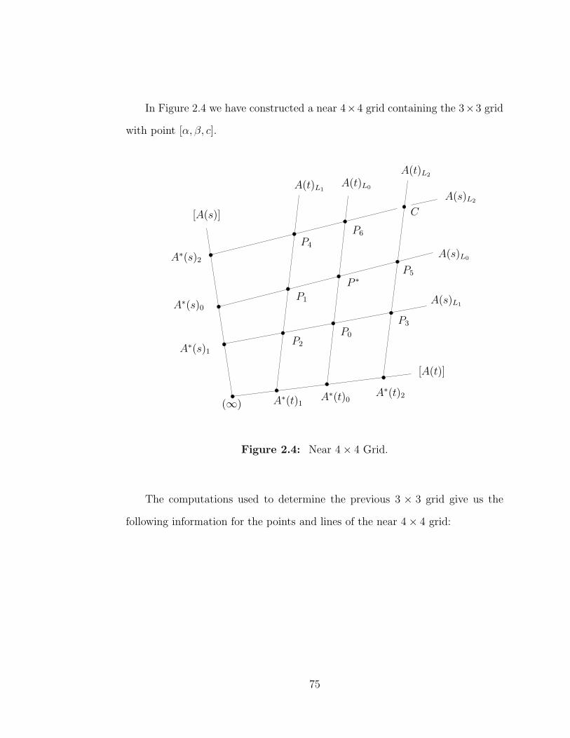
In Figure 2.4 we have constructed a near 4×4 grid containing the 3×3 grid
with point [α, β, c].
PSfrag replacements
P ∗
(∞)
[A(s)]
[A(t)]
A∗(s)0
A∗(s)1
A∗(s)2
A∗(t)0A∗(t)1
A∗(t)2
A(t)L0A(t)L1
A(t)L2
A(s)L0
A(s)L1
A(s)L2
P0
P1
P2
P3
P4
P5
P6
C
Figure 2.4: Near 4 × 4 Grid.
The computations used to determine the previous 3 × 3 grid give us the
following information for the points and lines of the near 4 × 4 grid:
75
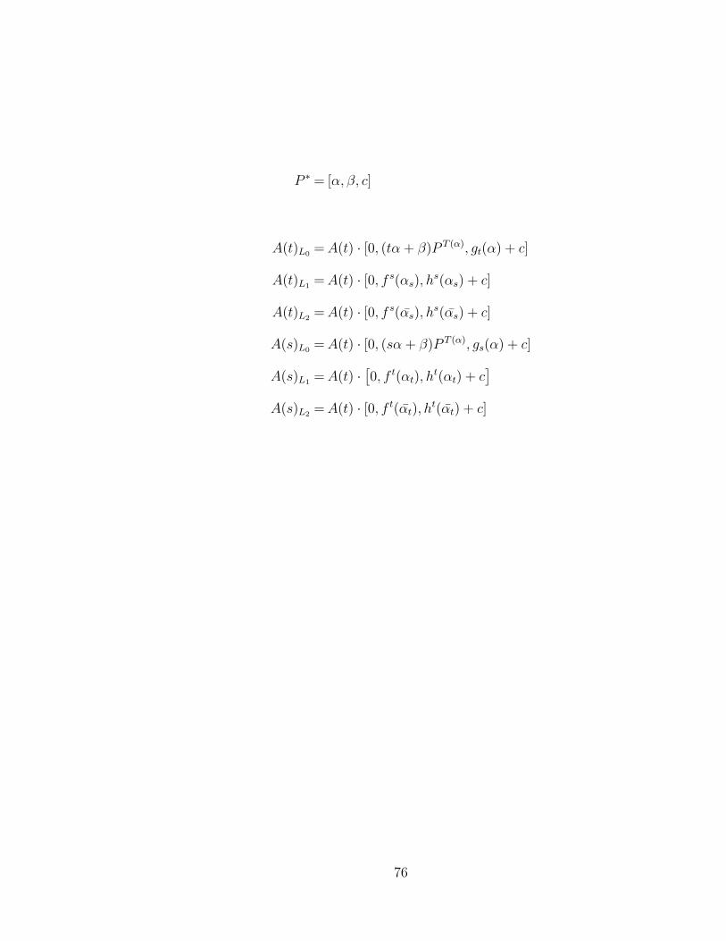
P ∗ = [α, β, c]
A(t)L0 = A(t) · [0, (tα + β)P T (α), gt(α) + c]
A(t)L1 = A(t) · [0, f s(αs), hs(αs) + c]
A(t)L2 = A(t) · [0, f s(αs), hs(αs) + c]
A(s)L0 = A(t) · [0, (sα + β)P T (α), gs(α) + c]
A(s)L1 = A(t) ·[
0, f t(αt), ht(αt) + c
]
A(s)L2 = A(t) · [0, f t(αt), ht(αt) + c]
76

P0t= [αt, tαt + (tα + β)P T (α+αt), gt(αt) + gt(α) + c]
P1s= [αs, sαs + (sα + β)P T (α+αs), gs(αs) + gs(α) + c]
P2 =ts
[
α∗, tα∗ + f s(αs)PT (α∗), gt(α
∗) + hs(αs) + c]
[
α∗, sα∗ + f s(αt)PT (α∗), gs(α
∗) + ht(αt) + c]
P3 =ts
[
α, tα + f s(αs)PT (α), gt(α) + hs(αs) + c
]
[
α, sα + f t(αt)PT (α), gs(α) + ht(αt) + c
]
P4 =ts
[
α, tα + f s(αs)PT (α), gt(α) + hs(αs) + c
]
[
α, sα + f t(αt)PT (α), gs(α) + ht(αt) + c
]
P5s=[
αs, sαs + (sα + β)P T (αs), gs(αs) + gs(α) + c]
P6t= [αt, tαt + (tα + β)P T (α+αt), gt(αt) + gt(α) + c]
Given this near 4 × 4 grid, the points P2, P3, and P4 tell us that we satisfy
the following conditions:
77

tα∗ + f s(αs)PT (α∗) = sα∗ + f t(αt)P
T (α∗)
tα + f s(αs)PT (α) = sα + f t(αt)P
T (α)
tα + f s(αs)PT (α) = sα + f t(αt)P
T (α)
Multiplying each equation by the appropriate power of P and adding equa-
tions we see that if we put
α = α∗P T (α+α) + αP T (α∗+α) + αP T (α∗+α) (2.4)
then we also satisfy the following condition:
tα + f s(αs)PT (α) = sα + f t(αt)P
T (α) (2.5)
Given this near 4 × 4 grid we also satisfy another set of conditions:
gt(α∗) + hs(αs) = gs(α
∗) + ht(αt)
gt(α) + hs(αs) = gs(α) + ht(αt)
gt(α) + hs(αs) = gs(α) + ht(αt)
Adding these equations together we get the equivalent condition:
gt(α∗) + gt(α) + gt(α) + hs(αs) = gs(α
∗) + gs(α) + gs(α) + ht(αt) (2.6)
78
We now ask if there is some point C which completes the 4× 4 grid to give
us property (G). This point would have to have the following coordinates:
Cts =
[
α, tα + f s(αs)PT (α), gt(α) + hs(αs) + c
]
[
α, sα + f t(αt)PT (α), gs(α) + ht(αt) + c
]
We note that if there is a solution it will be a unique solution.
This point is on both A(t)L2 and A(s)L2 if and only if
tα + f s(αs)PT (α) = sα + f t(αt)P
T (α) (2.7)
gt(α) + hs(αs) = gs(α) + ht(αt) (2.8)
If we let α = α as defined in equation 2.4 we have satisfied equation 2.7.
Then using equation 2.6 and the fact that
gt(α + α′) = gt(α) + gt(α′) + α
0 t
t 0
α′T
we see that satisfying equation 2.8 depends on satisfying
t (α∗Pα + α∗Pα + αP α) = s (α∗Pα + α∗Pα + αP α) .
79

Equivalently, since t 6= s, we must satisfy
α∗Pα + α∗Pα + αP α = 0
The point is that a solution to equations 2.7 and 2.8 does not depend on
the choice of the function gt. Then recalling that at least one choice gt produces
H(3, q2), which S.E.Payne has shown, see [8], has property(G) at the point (∞),
we see that we will satisfy equations 2.7 and 2.8 for any choice of gt.
Therefore, when the near 4× 4 grid contains lines [A(t)] and [A(s)] incident
with (∞), we have satisfied property(G) at the point (∞). Similar computations
show this is also true when the near 4 × 4 grid contains the lines [A(∞)] and
[A(t)], although we omit the details here.
2.11 A Theorem of Matt Brown
We now state a powerful result due to Matt Brown, see [5].
Theorem 2.11.1 Let S = (P,B, I) be a GQ(q, q2), q > 1, and assume that S
satisfies property(G) at some line l. Then S is the dual of a flock-GQ.
It follows that each EGQ constructed from the exotic elation groups of
H(3, q2) are flock-GQ.
80

2.12 The Final Push
Consider the following theorem from [28].
Theorem 2.12.1 Let S be a GQ and let H be a group of whorls about the point
x acting transitively on the set X = P \x⊥. The set of elations in H does not
form a group if and only if (at least) one of the following conditions is satisfied:
(1) There is a j ≥ 2 for which |fix(σ)| = j for some σ ∈ H.
(2) There is a proper thick sub-GQ of S containing x (and all the lines through
x) fixed pointwise by a non-identity element of H.
Theorem 2.12.2 Let S(F) be a non-classical flock generalized quadrangle of
order (q2, q), q > 1, q-even. Then the set of all elations about (∞) does form a
group.
Recall that φ is a whorl about (∞) that fixes more that one point in
P \ (∞). It follows that every “exotic” EGQ that we have constructed is
classical, and hence isomorphic to the Hermitian surface H(3, q2).
2.13 Suggested Problems
In this section we suggest how to further this research. First, and possibly
the most obvious question:
81

Question (1): Are there any new examples of EGQ that may be constructed
from these new groups?
We might also ask the following question:
Question (2): Are there conditions that guarantee an EGQ have non-
isomorphic elation groups?
The following conjecture was recently made by K. Thas.
Conjecture 2.13.1 (K. Thas) If Property(F ) does not hold for (S (p), G), then
S has non-isomorphic elation groups.
Property (F ) depends on whether each A∗ ∈ F ∗ is normal in the elation
group.
82

Appendix A. Theorems
Lemma A.1 dd∑
i=1
t2i ≥(
d∑
i=1
ti
)2
.
Proof: Taken from [1].
Set dm =
d∑
i=1
ti. Then after some straightforward manipulations we see that
0 ≤d∑
i=1
(m − ti)2 = −
(
d∑
i=1
ti
)2
d+
d∑
i=1
t2i
The result easily follows.
We will use this lemma to help prove the followng inequality due to Higman.
Theorem A.1 Let S = (P, B, I) be a GQ of order (s, t). Then s ≤ t2 and
dually t ≤ s2. Furthermore, t = s2 if and only if for some pair (x, y) of non-
collinear points every triad (x, y, w) has exactly s+1 centers if and only if every
triad of points has exactly 1 + s centers.
Proof: Taken from [22].
Now we let x, y be fixed non-collinear points with perp given by
x, y⊥ = z0, . . . , zt,
83
and let V = w1, . . . , wd be the set of all points such that x, y, w is a triad.
It follows that d = s2t− st− s+ t. Now for 1 ≤ i ≤ d, let ti be the number of zj
such that zj ∈ x, y, wi⊥. And for 0 ≤ i ≤ t + 1 let ni be the umber of triads
x, y, w with exactly i centers. Counting the total number of triads we get
t+1∑
i=0
ni = s2t − st − s + t
Now counting the total number of ordered pairs (w, z) such that z ∈ x, y, w⊥
we getd∑
i=1
ti =
t+1∑
i=0
ini = (t + 1)(t − 1)s = (t2 − 1)s
This follows since for each of the t + 1 points in x, y⊥ there are s points on
each of the t − 1 lines not through x or y.
Now counting the number of ordered triples (w, z, z′) such that w ∈
x, y, z, z′⊥ we get
d∑
i=1
ti(ti − 1) =t+1∑
i=0
i(i − 1)ni =
(
t + 1
2
)
· (t − 1) · 2 = (t2 − 1)t
This follows since for each of the(
t+12
)
ways to pick z, z′ from x, y⊥, there are
exactly t − 1 points (not in x, y⊥) which are the intersection of lines through
z, z′. But the triples are ordered and so it is obvious that
d∑
i=1
t2i = (t2 − 1)(s + t)
If we put dm =d∑
i=1
ti it follows from Lemma 1 that
84

0 ≤d∑
i=1
(m − ti)2 = t(s − 1)(s2 − t)
It is now an easy conclusion that t ≤ s2. Furthermore, if t = s2 we we must
have m = ti for each 1 ≤ i ≤ d and every triad has the same number of centers.
In this case there are s4 − s3 + s2 − s total triads each having the same number
k of centers. It follows that
k(s4 − s3 + s2 − s) =
d∑
i=1
ti = (s4 − 1)s = s5 − s
and we must have k = s + 1.
Theorem A.2 Let G be a group of order s2t and let F = A0, A1, . . . , At be a
family of t + 1 subgroups, each with order s, and let F∗ = A∗0, A
∗1, . . . , A
∗t be
another family of t + 1 subgroups, each having order st where Ai ≤ A∗i for each
0 ≤ i ≤ r. Then if we build the coset geometry S (∞) as prescribed above, S (∞)
is a GQ, having order (s, t), if and if properties K1 and K2 hold, where
K1 : AjAi ∩ Ak = id for all distinct i, j, k.
K2 : A∗jAi = id for all i 6= j.
Proof: We follow the proof in [20].
Two lines must be incident with at most one common point. We observe
that two distinct lines of type (ii) are incident only at the point (∞). Then for
85
each 0 ≤ j ≤ r, the cosets Ajg : g ∈ G partition the group elements, from
which it follows that two lines Ajg and Ajh may only be incident at a point A∗jg.
Next suppose that two points are incident with two lines Ajg and Aih, i 6= j.
Since any element in a coset Ajg or Aih can be chosen as a coset representative,
we can WLOG assume that the points are group elements g and h. But then
g, h ∈ Ajg ∩ Aih, or equivalently id, gh−1 ∈ Aj ∩ Ai. We have shown that no
two points are incident with two different lines if and only if Ai ∩ Aj = id for
each i 6= j. From now, we assume that the following property holds:
P1 : Ai ∩ Aj = id for all i 6= j.
Next we show that there are no triangles in the geometry. First, there can
be no triangle with vertex (∞) as no two points A∗i g and A∗
jh, i 6= j, are on a
common line, and no element g is incident with the point (∞). Furthermore,
since the cosets Ajg partition the group (and so intersect only on the line [Aj]),
there can be no triangle with vertices A∗jg, A∗
jh, and g, where A∗jg 6= A∗
jh. We
have two additional cases two consider.
First, suppose that A∗jg, g, and h are the vertices of a traingle. Then there
are cosets Ajg and Ajh which are contained in A∗jg, and the elements g, h are
in some coset Aig, i 6= j. See Figure A.1.
But this is if and only if g, h ∈ A∗jg∩Aig, or equivalently id, hg−1 ∈ A∗
j ∩Ai.
It follows that no triangles of this type occur if and only if the following property
holds.
86

PSfrag replacements
[Ai][Aj]
A∗jg
A∗i g
g
h
(∞)
AigAjg
Ajh
Figure A.1: P2 : A∗j ∩ Ai = id for all i 6= j.
P2 : A∗j ∩ Ai = id for all i 6= j.
From now assume that property P2 holds. We now have to show that there
are no triangles in the geometry that have g, h, and u as its vertices as in Figure
A.2.
PSfrag replacements
[Ai]
[Aj]
[Ak]
A∗i u
A∗kh
A∗jg
(∞)
gh
u
Figure A.2: P3 : AjAi ∩ Ak = id for all distinct i, j, k.
87

Assume that such a triangle exists. Then the following coset relationships
would hold.
Akh = Aku −→ hu−1 ∈ Ak
Aig = Aiu −→ gu−1 ∈ Ai
Ajg = Ajh −→ hg−1 ∈ Aj
But then (hg−1) · (gu−1) = hu−1 implies that |AjAi ∩Ak| ≥ 2. Next assume
that |AjAi ∩ Ak| ≥ 2. Then if id 6= g ∈ AjAi ∩ Ak we see that Ak = Akg and
g = ajai, giving us Ajai = Ajg and since g 6= ai (which follows since g ∈ Ak
and property P2 holds) the line Ajg has the points g and ai. But then the line
Ai intersects Ajg at the point ai and the line Ak at the point id, giving us a
triangle with vertices g, ai, and id. See Figure A.3.PSfrag replacements
Ai
Ajai = Ajg Ak = Akg
g
id ai
Figure A.3: P3 : AjAi ∩ Ak = id for all distinct i, j, k.
We have shown that no triangles exist, having vertices g, h and u, if and
only if the following property holds.
88

P3 : AjAi ∩ Ak = id for all distinct i, j, k.
From now on we assume that property P3 also holds. Our final step is to
show that given a line l and a point P not on L there is a unique point-line pair
(Q, m) such that PImIQIl.
First, if (∞) is not on a line Aig then there is unique line [Ai] and point A∗i h
such that (∞)I[Ai]IA∗i gIAig. Next suppose that the point A∗
i g is not incident
with a line Aih. Then then there is unique line [Ai] and point A∗i h such that
A∗i gI[Ai]IA∗
i hIAih. We have to consider two additional cases.
First, suppose that the point A∗i g is not incident with a line Ajh, i 6= j.
We need to find, as is pictured in Figure A.4, a point x ∈ A∗i g and a line Aig
(uniqueness follows from property P2) such that x ∈ Aig ∩ Ajh.
PSfrag replacements
[Ai] [Aj]Ajh
Aig
A∗i g
A∗jh
x
(∞)
Figure A.4: P4 : A∗i Aj = G for all i 6= j.
So Aig = Aix, Ajh = Ajx, A∗i g = A∗
i x, and A∗jh = A∗
jx, giving us x ∈
A∗i g ∩ Ajh. But, the cosets A∗
i g and Ajh were chosen arbitrarily, and so for
89

each g, h ∈ G there would have to be elements a∗i ∈ A∗
i and aj ∈ Aj such that
a∗i g = ajh, or gh−1 = (a∗
i )−1aj ∈ A∗
i Aj. We have shown that this case holds if
and only if the following property holds.
P4 : A∗i Aj = G for all i 6= j.
Obviously, for each g ∈ G, there is a unique line containing g and incident
with a point on each line [Ai]. So finally, suppose that the point g is not incident
with a line Aih, that is g 6∈ Aih. First define
Ω = ∪Ai : 0 ≤ r ≤ r
Since P1 and P2 hold, each coset of Ai different from Ai but contained in A∗i
is disjoint from Aj, and we have the following
A∗i ⊆ Ai ∪ Aig : Aig ∩ Ω = ∅
Since g 6∈ Aih, we can WLOG assume that the point is id 6∈ Aig. First
consider the case g ∈ A∗i \ Ai. Here A∗
i g = A∗i is a point on the lines Aig and
Ai, the second of which is collinear with the point id.
So we may assume that g 6∈ A∗i . We need to find a line Aj such that
|Aj ∩ Aig| = 1 . So there must be an i 6= j such that Aj ∩ Aig 6= ∅.
So if Aig is a coset of Ai disjoint from Ω, it must be that Aig ⊂ A∗i . But we
have already shown that A∗i ⊆ Ai ∪ Aig : Aig ∩ Ω = ∅. So assuming that P1
through P4 holds, this case holds if and only if the following property holds.
90

PSfrag replacements[Ai] Aig
A∗i g id
Figure A.5: P5 : A∗i = Ai ∪ Aig : Aig ∩ Ω = ∅
PSfrag replacements
[Ai] [Aj]Aig
Ai
Aj
A∗i g
A∗i
A∗j
id
(∞)
Figure A.6: P5 : A∗i = Ai ∪ Aig : Aig ∩ Ω = ∅
P5 : A∗i = Ai ∪ Aig : Aig ∩ Ω = ∅
Looking back at the properties P1, . . . , P5 it is easy to see that P2 implies
P1, and since G is finite, P2 also implies P4. Hence we need only assume that
properties P2, P3, and P5 hold. It turns out that P5 holds if and only if r = t.
We show this, and that the coset geometry is a GQ(s, t), if and only if r = t
and properties P2 and P3 hold. Assuming that P2 and P3 hold we need the
91

following lemmas.
Lemma A.2 Let g ∈ G and i 6= j. Then |Ajg ∩ Ai| ≤ 1.
Proof: (Lemma A.2) Suppose that both x, y ∈ Ajg∩Ai. Then x = ajg = ai
and y = a′jg = a′
i. Hence, g = a′ia
′−1j = aia
−1j , and a−1
i a′i = a−1
j a′j 6= id and we
have violated property P1, and so also P2.
Lemma A.3 Let g ∈ Ω \ Aj. Then Ajg ∩ Ω = g.
Proof: (Lemma A.3). Notice that g ∈ Ai, for some i 6= j, so g = ai. But
then Aj 6= Ajg ⊂ AjAi, whose intersection with every other Ak is the identity.
Since id 6∈ Ajg we must have Ajg intersecting Ω only in the element g.
We next claim that if S = (P, B, I) is the coset geomtry defined above, then
assuming properties P2 an P3, property P5 holds if and only if r = t. As there
are r + 1 subgroups of order s in Ω, it is easy to see that |Ω \ Aj| = r(s − 1).
This means that there are exactly 1+r(s−1) distinct cosets of Aj that intersect
Ω, and so there are st − [1 + r(s − 1)] cosets of Ai that are disjoint from Ω. If
we assume that P5 holds we get |A∗i | = st = s + s[st − 1− r(s− 1)] which gives
us st(s − 1) = rs(s − 1), which holds if and only if r = t.
We relabel properties P2 and P3, as K2 and K1 respectively. Now with
r = t it is trivial to count that each line is incident with exactly s + 1 points,
and that each point is on exactly t + 1 lines. This completes the proof.
92

Theorem A.3 Using the Kantor family (G⊗,J (C),J ∗(C)) as prescribed above,
let S = GQ(C) be the EGQ. Then S is a GQ(q2, q) isomorphic to the Hermitian
surface H(3, q2).
Proof: See [22].
Theorem A.4 The quadrangle H(3, q2) is isomorphic to the point-line dual of
Q(5, q).
Proof: Taken from [22].
Let Q be an elliptic quadric of PG(5, q), and extend PG(5, q) to PG(5, q2).
Then the extension of Q is an hyperbolic quadric Q+ in PG(5, q2). Hence, Q+
is the Klein quadric corresponding to the lines of PG(3, q2). So to Q in Q+
there correspond a set V of lines in PG(3, q2), To a given line L of Q(5, q) there
correspond q+1 coplanar lines through a point x of PG(3, q2). Let H be the set
of points on the lines of V . Then with each point of Q(5, q) there corresponds
a line of V , and with each line of Q(5, q) there corresponds a point of H. With
distinct lines L, L′ of Q(5, q) correspond distinct points x, x′ of H (a plane of Q+
contains at most one line of Q). Since each point y of Q(5, q) is on q2 + 1 lines
of Q(5, q), these q2 +1 lines are mapped onto the q2 +1 points of the image of y.
Hence we obtain an anti-isomorphism from Q(5, q) onto the structure (H, V, I),
where I is the natural incidence relation. So (H, V, I) is a GQ of order (q2, q)
embedded in PG(3, q2). Then the following result of F. Buekenhout and C.
Lefevre guarantees that (H, V, I) must be H(3, q2).
93

Theorem A.5 (Buekenhout, Lefevre) [4] A projective GQ S = (P,B, I)
with ambient space PG(n, q) must be obtained in one of the following ways:
(i) There is a unitary or symplectic polarity π of PG(n, q), n = 3 or 4, such
that P is the set of absolute points of π and B is the set of totally isotropic
lines of π.
(ii) There is a nonsingular quadric Q of projective index 1 in PG(n, q), n = 3,
4 or 5, such that P is the set of points of Q and B is the set of lines on Q.
Proof: See [22].
Theorem A.6 If f : GF (q) 7→ GF (q) is an additive function, then
f(x) = a0x + a1xp + a2x
p2
+ · · ·+ ae−1xpe−1
where ai ∈ GF (q).
Proof: Let q = pe and f : GF (q) 7→ GF (q) be the GF (q)-additive (and
GF (p)-linear) function
f(x) = a0x + a1xp + a2x
p2
+ · · ·+ ae−1xpe−1
Suppose that f(x) = 0 for all x ∈ GF (q). Then since the deg[f(x)] = e − 1
it must be the zero polynomial, and so a0 = a1 = · · · = ae−1 = 0. Hence, the
set x, xp, . . . , xpe−1 are linearly independent in the additive group (or vector
space) of GF (p)-linear functions and so form a basis of a subspace of dimension
94
e. It follows that there are exactly qe distinct functions of this form.
Now consider the entire additive group of operators T : GF (q) 7→ GF (q)
where we think of the field as an e-dimensional vector space over Zp. The
dimension of this vector space is the same as the dimension of all e× e matrices
over GF (p) which is e2 (since there is a basis of matrices each with a single
non-zero entry). Since the matrices have coefficients in Zp there are exactly
pe2= (pe)e = qe linear operators T . But this is exactly the same number of
GF (q)-additive functions (which are GF (p)-linear). Therefore, we have found
all GF (q)-additive functions.
Theorem A.7 Let gt(α) be a function from GF (q)×GF (q) into GF (q). Then
there is a distinct polynomial associated with gt(α) of the form
gt(α) =∑
0≤j,k≤q−1
cj,kαk1α
j2, where cj,k ∈ GF (q)
Proof: Any polynomial of the form
gt(α = (α1, α2)) =∑
0≤i,j≤q−1
ci,jαi1α
j2, where ci,j ∈ GF (q)
is a function from GF (q) × GF (q) 7→ GF (q). We show that no two of these
polynomials represent the same function.
Suppose that we have
ft(α) =∑
0≤i,j≤q−1
ci,jαi1α
j2 and gt(α) =
∑
0≤i,j≤q−1
di,jαi1α
j2
95
Then supppose that
0 = h(α) = ft(α) − gt(α)
=∑
0≤i,j≤q−1
ci,jαi1α
j2 −
∑
0≤i,j≤q−1
di,jαi1α
j2
=∑
0≤i,j≤q−1
(
ci,j − di,j
)
αi1α
j2 for all α1, α2 ∈ GF (q)
If we fix α2 = a then we get
0 = ht(α) =∑
0≤i,j≤q−1
(
ci,j − di,j
)
αi1a
j
=
q−1∑
i=0
(
q−1∑
j=0
(
ci,j − di,j
)
aj
)
αi
for all α ∈ GF (q).
But ht(α) is a polynomial in α with degree less than q and so having q roots
it must be the zero polynomial. It follows that
0 =
q−1∑
j=0
(
ci,j − di,j
)
aj for all a ∈ GF (q)
But this is again a polynomial in a ∈ GF (q) of degree less than q with q
roots and therefore we get ci,j = di,j for all 0 ≤ i, j ≤ q − 1, and no two distinct
polynomials of this form will result in the same functional from GF (q)×GF (q)
96

into GF (q).
But now recall that there are exactly qq2functions from GF (q)×GF (q) into
GF (q) and this is the same number of distinct polynomials
ft(α) =∑
0≤j,k≤q−1
cj,kαk1α
j2, where cj,k ∈ GF (q),
mapping GF (q) × GF (q) into GF (q). This completes the proof.
97

Appendix B. The Hermitian Surface: A Unitary Representation
Let q = 2e and consider the projective space PG(V ), where V is an (n+1)-
dimensional vector space over GF (q2). Without loss of generality we can choose
the Hermitian form H : V × V 7→ GF (q) where
H(x, y) = x1yq4 + x2y
q3 + x3y
q2 + x4y
q1
That is, H(x, y) = xA(yq)T , where
A =
0 0 0 1
0 0 1 0
0 1 0 0
1 0 0 0
The set of all absolute points and totally isotropic lines of PG(3, q2) forms the
Hermitian surface H(3, q2). This is a GQ of order (q2, q).
The projective unitary group, denoted PGU(4, q2), is the subgroup of
PGL(4, q2) preserving the Hermitian form. So PGU(4, q2) =
B ∈ PGL(4, q2) :
BA(Bq)T = kA, k ∈ GF (q2)
and∣
∣PGU(4, q2)∣
∣ = q6(q + 1)(q3 + 1)(q4 − 1). If
we adjoin the complete set of automorphisms of GF (q2) to PGU(4, q2), we
form the group PΓU(4, q2). This is the complete group of collineations of
the Hermitian surface. Then |PΓU(4, q2)| = |Aut(GF (q2))| · |PGU(4, q2)| =
2e · q6(q + 1)(q3 + 1)(q4 − 1).
98

The binary operation ∗ in PΓU(4, q2) is composition of maps. Consider a
point x = (x1, x2, x3, x4) ∈ H(3, q2) and elements g = A σ and g′ = A′ σ′ in
PΓU(4, q2). We compute xg·g′ in a number of steps.
xA =
(
4∑
i=1
x1a1,i , . . .
)
xAσ =
(
4∑
i=1
xσ1aσ
1,i , . . .
)
xAσ∗A′σ′
=
(
j=1∑
4
[
4∑
i=1
xσ·σ′
1 aσ·σ′
1,i
]
(a′1,j)
σ′
, . . .
)
=
(
j=1∑
4
[
4∑
i=1
x1a1,i
]
(a′1,j)
σ−1
, . . .
)σ·σ′
It follows that in PΓU(4, q2), we have the group product
A σ ∗ A′ σ′ =(
A · (A′)σ−1)
(σ · σ′).
Theorem B.1 The set of all upper triangular matrices in PGU(4, q2) with ones
on the diagonal forms a Sylow2 subgroup of PGU(4, q2) having order q6.
Proof: Consider the matrix
B =
1 a b c
0 1 d e
0 0 1 f
0 0 0 1
99

Then
BA(Bq)T =
abq + baq + c + cq b + adq + eq a + f q 1
e + daq + bq d + dq 1 0
f + aq 1 0 0
1 0 0 0
and B ∈ PGU(4, q2) if and only if the following conditions hold: d + dq = 0,
abq + baq + c + cq = 0, f + aq = 0, and e + daq + bq = 0. It easily follows
that there are q6 such matrices in PGU(4, q2), and this set of matrices forms a
Sylow2 subgroup of PGU(4, q2).
We will call this group Sylow2 subgroup U2. If we then adjoin to U2 all
of the field automorphisms of GF (q2) that have order a power of 2 we form a
Sylow2 subgroup (that we will denote Γ2) of PΓU(4, q2) having order (#aut) ·q6.
The group Γ2 is the stabilizer of the flag in H(3, q2) having point p =
(0, 0, 0, 1) and line x1 = x2 = 0. We next construct the standard elation group
about p.
If P is the set of all points of H(3, q2), we have P \ p⊥ = (1, α, β, µ) ∈
PG(3, q2) : µ + µ + αβ + αβ = 0. So there are q5 points in P \ p⊥,
since αβ + αβ ∈ GF (q) and µ + µ is the relative trace function mapping
µ ∈ GF (q2) to GF (q). Furthermore, p⊥ \ p = (0, 1, a, b) : a ∈ GF (q), b ∈
GF (q2) ∪ (0, 0, 1, c) : c ∈ GF (q2), giving us all q3 + q2 + 1 points in p⊥.
100

The group of matrices
Mp =
1 α β µ
0 1 0 β
0 0 1 α
0 0 0 1
∈ GL(4, q2) : µ + µ + αβ + αβ = 0
is an elation group about p, as this group acts regularly on the set of points
in P \ p⊥(
the Mp-orbit of (1, 0, 0, 0) is the set of points (1, α, β, µ) :
µ + µ + αβ + αβ = 0)
and fixes every line through p.
Consider the group G = (α, µ, β) : α, βµ ∈ GF (q2) : µ + µ + αβ + αβ = 0
with binary operation
(α, µ, β) · (α′, µ′, β) = (α + α′, µ + µ′ + αβ ′ + βα′, β + β ′)
This group is the standard elation group of H(3, q2) (when viewed as an EGQ).
If we form the map
T : (α, µ, β) 7→
1 α β µ
0 1 0 β
0 0 1 α
0 0 0 1
we see that T[
(α, µ, β) · (α′, µ′, β ′)]
= T [(α, µ, β)] · T [(α′, µ′, β ′)]. Therefore, Mp
is the standard elation group about p.
Next consider the Hermitian preserving involution
φ : (a, b, c, d) 7→ (a, b, c, d).
101

Then, φ fixes p. Moreover, φ : (0, 0, 1, w) 7→ (0, 0, 1, w), and if y ∈ GF (q) then
φ : (0, 1, y, w) 7→ (0, 1, y, w). Since all Hermitian lines through p will be either
Ly = (0, 1, y, 0)+w(0, 0, 0, 1)∪(0, 0, 0, 1) or L′ = (0, 0, 1, 0)+w(0, 0, 0, 1)∪
(0, 0, 0, 1), we see that φ fixes all lines through p. Yet φ fixes the set of points
in (1, α, α, µ) : α, µ ∈ GF (q), which are in P \ p⊥. So φ is a whorl about p,
and Mp × 〈φ〉 is a Sylow2 subgroup of the group of whorls about p.
102

REFERENCES
[1] L. Batten. Combinatorics of Finite Geometries, second edition. Cam-bridge University Press, Cambride England. 1997.
[2] A. Beutelspacher and U. Rosenbaum. Projective Geometry. Cam-bridge University Press, Cambridge, England. 1998.
[3] R.C. Bose. Strongly regular graphs, partial geometries and partially bal-anced designs. Pacific Lournal of Mathematics. 13 pp. 389-419. 1963.
[4] F. Buekenhout and C. Lefevre. Generalized quadrangles in projectivespaces. Arch. Math. 25 pp.540-552. 1974.
[5] M. Brown. Projective ovoids and generalized quadrangles. Transactionsof the American Mathematical Society. 200?.
[6] P.J. Cameron Projective and Polar Spaces QMW Maths Notes 13. QueenMary and Westfield College, London E1 4NS.
[7] X. Chen. On the groups that generate skew-translation generalized quad-rangles. Unpublished manuscript.
[8] I. Cardinali and S.E. Payne The q-clan geometries with q = 2e.http://www-math.cudenver.edu/ spayne/. 2002.
[9] P. Dembowski. Finite Geometries. Springer-Verlag, Berlin, Germany,1968.
[10] W. Feit and G. Higman. The existence of certain generalized polygons.Journal of Algebra, 1:114-131, 1964.
[11] D.G. Glynn The hering classification for inversive planes of even order.Simon Stevin 58, 319-353, 1984.
[12] L.C. Grove. Classical Groups and geometric Algebra, volume 39 of Grad-uate Studies in Mathematics. American Mathematical Society, Providence,Rhode Island. 2001.
103

[13] D.G. Higman. Partial geometries, generalized quadrangles and stronglyregular graphs. Atti convegno di geometria e sue applicazioni (ed. A. Bar-lotti). Perugia, pp. 263-293. 1971.
[14] W. Kantor. Genralized polygons, SCABs and GABs. Lecture Notes inMathematics, Vol 1181. Springer, Berlin. 1986.
[15] M. Law and T. Penttila. Flocks, ovals and generalized quadrangles(Four Lectures in Napoli). 2000.
[16] C.M. O’Keefe and T. Penttila. Characterisations of flock quadran-gles. Geometriae Dedicata, Vol. 82 pp.171-191. 2000.
[17] S.E. Payne. A new infinite family of generalized quadrangles. Congr. Nu-mer., Vol. 49 pp. 115-128. 1985
[18] S.E. Payne. An essay on skew translation generalized quadrangles. Ge-ometriae Dedicata, 32:93-118, 1989.
[19] S.E. Payne. Elation generalized quadrangles. Hand written notes.http://www-math.cudenver.edu/∼spayne/. 1994.
[20] S.E. Payne. Lectures on finite generalized quadrangles. http://www-math.cudenver.edu/∼spayne/. 2000.
[21] S.E. Payne. Trace equation over finite fields of characteristic 2. Notes fromUCD geometry seminar. 2004.
[22] S.E. Payne and J. Thas. Finite Generalized Quadrangles, volume 110 ofResearch Notes in Mathematics. Pitman Publishing Inc., Boston 1984.
[23] S.E. Payne and K. Thas. Notes on Elation Generalized Quadrangles.European Journal of Combinatorics, Vol. 24 pp.969-981. 2003.
[24] Tim Penttila. Private Communication. 2004
[25] T. Penttila and C. Praeger. Ovoids and Translation Ovals. J. LondonMath. Soc., (2) 56 (1997) 607-624.
[26] J. Rotman. An Introduction to the Theory of Groups, Fourth edition.Springer-Verlag New York, Inc. 1995.
[27] J.A. Thas. Generalized quadrangles and flocks of cones. European Journalof Combinatorics, Vol. 8 pp. 441-452. 1987.
104

[28] K. Thas and S.E. Payne. Foundations of generalized quadrangles. Eu-ropean Journal of Combinatorics, Vol. 27 pp.51-62. 2006.
[29] J. Tits. Sur la trialite et cetains groupes qui s’en deduisent. Inst. HautesEtudes Sci. Publ. Math., 2:14-60, 1959.
[30] H. Van Maldeghem. Generalized Polygons, volume 93 of Monographs inMathematics. Birkhauser Verlag, Berlin 1998.
105