ELASTIC PROPERTIES OF SALT:

LABORATORY MEASUREMENTS, WELL-LOG ANALYSIS, AND

A SEISMIC SURVEY OVER THE HOCKLEY SALT MINE, TEXAS

__________________

A Thesis

Presented to

the Faculty of the Department of Earth and Atmospheric Sciences

University of Houston

__________________

In Partial Fulfillment

of the Requirements for the Degree

Master of Science

__________________

By

Jingjing Zong

August 2014

ii

ELASTIC PROPERTIES OF SALT:

LABORATORY MEASUREMENTS, WELL-LOG ANALYSIS, AND

A SEISMIC SURVEY OVER THE HOCKLEY SALT MINE, TEXAS

_________________________________________________

Jingjing Zong

APPROVED:

_________________________________________________

Dr. Robert Stewart, Committee Chair

Department of Earth and Atmospheric Sciences

_________________________________________________

Dr. Aibing Li, Committee member

Department of Earth and Atmospheric Sciences

_________________________________________________

Dr. Scott Leaney, Committee member

Schlumberger

_________________________________________________

Dean, College of Natural Sciences and

Mathematics

iii

Acknowledgements

I am especially thankful to my supervisor, Dr. Robert Stewart, for his insightful

suggestions on my research, for his guidance throughout the Master's program, and for

his willingness to share the wisdom of life with me. I would like to thank the rest of my

thesis committee, Dr. Aibing Li and Dr. Scott Leaney, for their encouragement and

invaluable input to my work. I would like to express my special thanks to Dr. Fred

Hilterman for his generous donation of log data as well as thoughtful instructions. I also

thank Dr. Nikolay Dyaur for patient assistance and instructions to carry out this

wonderful project.

Secondly, I would also like to thank all the Allied Geophysics Laboratory (AGL)

personnel who helped me in software and theoretical developments.

I thank substantially Dr. Michael Myers and Daniel Coleff of the University of Houston,

for the salt sample CT scanning and confining pressure tests. Also, I thank Rock Physics

Laboratory of UH for the assistance in measuring salt sample velocities with confining

pressure.

I want thank my parents for supporting me to finish this project both spiritually and

materially. Also thank all my friends who supported me unconditionally all the way along

and gave me great comfort when I felt helpless.

I am grateful to all those who helped me in my project.

iv

ELASTIC PROPERTIES OF SALT:

LABORATORY MEASUREMENTS, WELL-LOG ANALYSIS, AND

A SEISMIC SURVEY OVER THE HOCKLEY SALT MINE, TEXAS

__________________

An Abstract of a Thesis

Presented to

the Faculty of the Department of Earth and Atmospheric Sciences

University of Houston

__________________

In Partial Fulfillment

of the Requirements for the Degree

Master of Science

__________________

By

Jingjing Zong

August 2014

v

Abstract

Salt plays a significant part in the geology of the Gulf of Mexico area (GoM). Numerous

basins in the world have undergone evaporation sequences that have deposited vast

quantities of salt. Sometimes these deposits have remained largely undeformed, which

can lead to anisotropic crystal growth, while other salt deposits have undergone

significant movement and extrusion. In this thesis, I use lab measurements, well-log data,

and surface seismic to determine the properties of salt crystal and rocks.

In the lab, we have undertaken ultrasonic measurements on salt samples from various

locations. The pure halite crystals from the Goderich salt mine, Canada, demonstrate

shear-wave splitting and compressional-wave variations which indicate cubic anisotropy.

The stiffness values calculated for that are C11 = 48.7 GPa, C44 = 13.1 GPa , and C12 =

11.9 GPa. Our samples from the Hockley and the Bayou salt mine have fractures, and

aligned domains, but no obvious anisotropy. The density ranges from 2.16 - 2.22 g/cc.

The confining pressure experiments are conducted on the Louisiana salt cores. The

velocities under 0 - 4000 psi are 4.4 - 4.8 km/s for P-waves and 2.5 - 2.8 km/s for S-

waves.

For a 1 km-thick numerical halite model, the travel-time difference caused by cubic

anisotropy is up to 20 ms for P-waves based on the calculated stiffness values.

We analyzed 142 well-log from boreholes drilled through salt in the GoM. We find an

empirical relationship for P-wave velocity of salt V (km/s) versus depth D (km)：

vi

𝑉 = 4.41 + 0.0145𝐷

The RMSE of the fit is 0.10 km/s. This variability may be useful for modeling velocities

in “dirty” or inhomogeneous salt deposits. For salt density vs. velocity, our log data are

similar to Gardner’s, although we find a cluster, not a monotonic relationship.

We acquired a 1.2 km seismic line over Hockley Salt Mine. From refraction crossover

analysis of one shot gather, we find depth for the top of anhydrite with the stacking

velocity of 5.5 km/s occurs around 50 m (164 ft).

These studies of elastic properties of salt provide more information for salt velocity model

building and a general understanding of salt properties.

vii

Contents

1 Introduction .................................................................................................................... 1

1.1 Background and motivation ...................................................................................... 1

1.2 Thesis objective and structure ................................................................................... 4

1.3 Data sets used in thesis ............................................................................................. 5

2 Ultrasonic lab measurements ........................................................................................ 6

2.1 Salt property introduction ......................................................................................... 6

2.2 Anisotropy parameter estimation .............................................................................. 9

2.3 Salt samples ............................................................................................................ 10

2.4 Measurement of Vp and Vs .................................................................................... 14

2.5 Discussion ............................................................................................................... 33

3 Empirical relationships of salt in the Gulf of Mexico coast from well-log data ..... 37

3.1 Introduction ............................................................................................................. 37

3.2 Salt velocity versus depth ....................................................................................... 44

3.3 Predicted salt velocity versus pressure ................................................................... 50

3.4 Salt velocity versus density ..................................................................................... 52

4 Numerical modelling of salt ........................................................................................ 55

viii

4.1 Introduction ............................................................................................................. 55

4.2 Phase and group velocities distribution in space .................................................... 55

4.3 Quantification of travel time difference caused by cubic salt ................................. 57

5 Seismic survey over the Hockley salt dome ............................................................... 62

5.1 Introduction ............................................................................................................. 62

5.2 Geology and map .................................................................................................... 63

5.3 Seismic line layout .................................................................................................. 64

5.4 Data processing and imaging .................................................................................. 66

6 Conclusions ................................................................................................................... 75

References ........................................................................................................................ 78

Appendix .......................................................................................................................... 82

1

Chapter 1

Introduction

1.1 Background and motivation

With some of the world’s largest oil discoveries in recent years being located below or

close to salt bodies (Landrø et al., 2011), considerable attention from the energy industry

is now focusing on pre-salt and sub-salt imaging. Salt has generally been described as an

isotropic medium in regular seismic processing. Whether such a simplification is

universally reliable needs to be investigated.

This thesis studies the elastic properties of salt, including its anisotropy. According to

composition, salt can be classified into two groups, impure and pure salts. From the

geological perspective, as seawater evaporates, the concentration of carbonates, sulphates,

and chlorides increases to the point where one or more salts will precipitate. Salt crystals

grow in certain trends where salt was originally deposited in a stable environment.

Different types of salt have various original depositional environment and diagenesis

histories. A pure, undeformed salt crystal (halite) has cubic symmetry which is elastically

anisotropic (Pauling, 1929). Other deformed pure salts are classified into three types by

Sun (1994) in terms of possible seismic anisotropy:

2

1. Detrital-framework salt, the framework of grains with point contacts establishes a

primary detrital texture in evaporites as elastic rocks. The salt layer exhibits isotropic

features;

2. Burial metamorphic salt, this type of salt can be anisotropic or isotropic. It can

have strongly preferred crystal orientation. It also can be altered by the temperature and

pressure due to burial. If strained thermo-mechanically, the texture of salt dome could

display anisotropic properties;

3. Crystal-oriented salt, this kind of salt often represents growth in a stable

environment. It is layered and has syntaxially grown crystalline framework salt consisting

of vertically oriented and vertically elongated crystals without recrystallization.

Situations are more complicated for deformed, impure salt rocks. Impure salts are those

in which salt crystals are mixed with clastic deposits. This is due to intra-sedimentary

growth of salt (Sun, 1994). Salt rock is a special type of sedimentary rock which has high

velocity (4.5 to 5.0 km/s) and low density (2000 to 2200 kg/m3). It is buoyant (in denser

material) and deformable which allows it to flow upwards and laterally with relative ease.

An important consequence of such flow is that the constituent crystals within the salt

body can align, thereby generating an effective seismic anisotropy (Raymer et al., 2000).

The lineation of salt is better developed in anhydrite-bearing salt (Balk, 1953). On the

other hand, layering of anhydrite, dust, and other impurities is another possible reason for

anisotropy (Balk, 1953).

3

Given the possibilities of salt anisotropy, it is prudent to review how accurate is the

isotropy assumption; especially, when we are interested in accurate pre-salt and sub-salt

imaging.

There are a number of major salt basins around the world (Lane, 2008). The Gulf of

Mexico (GoM) crustal region hosts the major salt basin in North America. The main

GoM salt accumulation occurred in the Jurassic, but accentuation and modification of

these features continued over time. Salt deposits are originally formed horizontally as salt

beds in ancient bodies of water, and then buried deeply beneath sediments. Tectonic

forces in the earth subsequently deformed these salt beds (Salvador, 1991). The

overlaying Upper Jurassic marine strata formed an aggrading, slowly prograding,

carbonate wedge that loaded the salt fairly uniformly in the Gulf of Mexico area (Bishop,

1968).

Salt domes are common structures caused by tectonic deformation and salt movement.

The dome’s salt stock and cap rock are generally enclosed within sedimentary deposits.

The main evaporite mineral is halite. The cap rock is generally composed of sulfate and

carbonate minerals. Salt domes can provide structural deformation and traps for oil and

gas accumulations. They are also useful for storage as well as seals for reservoirs. There

is a thick belt of salt domes (greater than 6 km deep) located beneath the Gulf of Mexico

coast surface. Thorough exploration has been conducted over many salt structures in the

Gulf of Mexico (Hamlin, 2006).

4

1.2 Thesis objective and structure

I investigate the salt properties of pure halite from Goderich, Canada and salt rocks from

domes in the GoM region in the lab. I also use well-log data from 142 wells through salt

in the Gulf of Mexico area as well as 2D surface seismic data acquired over the Hockley

Salt Mine in my thesis.

In Chapter 2, I introduce the lab measurements for different salt samples. Both P- and S-

wave velocities are recorded in various polarization directions. From the lab

measurements, I evaluate the anisotropy properties for pure halite and impure, deformed

salt samples. I am able to conclude about the anisotropy type for pure halite and further

calculate anisotropy parameters.

More salt properties in the Gulf of Mexico are studied in Chapter 3. Based on 142 wells

drilled through salt along the GoM coast, empirical relationships of salt velocity with

density and depth are generated and discussed. These relationships are given to provide

velocity models for pre-salt and subsalt imaging.

In Chapter 4, numerical models are built to evaluate potential travel time differences

caused by cubic anisotropy. I first build two single-layered numerical velocity models:

one basic model is isotropic while another is cubic-symmetric anisotropy. The anisotropy

parameters used are calculated from the laboratory measurements.

In Chapter 5, a 1.2 km 2D surface seismic survey in Hockley Salt Mine is analyzed. The

seismic profile provides a velocity model of a typical salt dome in the Gulf of Mexico

area. The cap rock and the top of salt are interpreted.

5

1.3 Data sets used in thesis

1.3.1 Ultrasonic laboratory measurements of salt samples

The salt compressional and shear velocities shown in Chapter 2 were measured by

ultrasonic instruments at the Allied Geophysics Laboratory (AGL), University of

Houston. Salt samples include pure salt crystal from Sifto's Goderich Mine, Canada, salt

core from Bayou Corne Salt Dome, Louisiana and salt samples from Hockley Salt Mine,

Houston. The ultrasonic tests under confining pressure are taken in collaboration with Dr.

M. Myers in Petroleum Engineering and the Rock Physics Lab at UH.

1.3.2 Well-log data through salt in the Gulf of Mexico

A general statistic investigation of salt properties in the upper Gulf of Mexico over 142

well-logs are discussed in Chapter 3. Some empirical relationships between velocity

versus depth, pressure and density are built based on the log data. The well-log data in

Chapter 3 are provided by Dr. Fred Hilterman and Geokinetics, Houston.

1.3.3 Surface seismic data over the Hockley Salt Mine, TX

To further investigate salt velocities and emplacement structure, a 1.2 km 2D surface

seismic line was shot over the Hockley Salt Mine, TX. It was conducted by the Allied

Geophysics Laboratory (AGL), University of Houston with the assistance of United Salt

Corporation, Houston. Detailed acquisition as well as interpretation is given in Chapter 5.

6

Chapter 2

Ultrasonic lab measurements

2.1 Salt property introduction

Pure salt (NaCl) is a crystalline mineral made of cube-shaped crystals composed of two

elements: sodium and chloride. Rock salt deposits are typically formed by the

evaporation of salty water (such as sea water) which contains dissolved Na+ and Cl- ions.

Compared to pure halite crystals (NaCl), rock salt can have impurities of gypsum (CaSO4)

and sylvite (KCl).

2.1.1 Physical properties

Pure salt mineral is a crystalline solid with cubic symmetry form. The physical properties

of pure halite are listed on Table 2.1.

Properties of Pure Sodium Chloride:

Molecular weight - NaCl 58.4428

Atomic weight - Na 22.989768 (39.337%)

Atomic weight - Cl 35.4527 (60.663%)

Freezing point of eutectic mixture -21.12° C (-6.016°F)

Crystal form Isometric, Cubic

Color Clear to White

Index of refraction 1.5442

Density or specific gravity 2.165 (135 lb/ft3)

Angle of repose (dry, ASTM D 632 gradation) 32°

Melting point 800.8° C (1,473.4° F)

Boiling point 1,465°C (2,669° F)

Hardness (Moh's Scale) 2.5

Critical humidity at 20 °C, (68° F) 75.3%

pH of aqueous solution neutral

Table 2.1. Physical properties of pure sodium chloride (Lane, 2008).

7

The cubic crystal’s size varies broadly. It depends on the formation environment. All

sodium chloride is crystalline under strong magnification. Large cubic crystals (5-8 cm in

diameter) are common in salt domes and can be recognized by eye. They cleave into

perfect cubes when struck.

The purity of salt depends on salt type: rock salt, evaporites and so on. Halite in rock salt

ranges from 95% to 99% and higher than 99% in evaporites.

2.1.2 Salt anisotropy

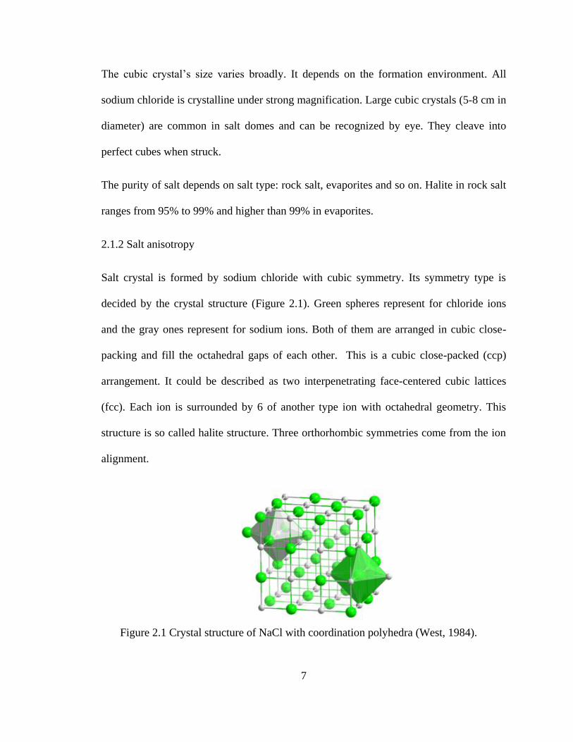
Salt crystal is formed by sodium chloride with cubic symmetry. Its symmetry type is

decided by the crystal structure (Figure 2.1). Green spheres represent for chloride ions

and the gray ones represent for sodium ions. Both of them are arranged in cubic close-

packing and fill the octahedral gaps of each other. This is a cubic close-packed (ccp)

arrangement. It could be described as two interpenetrating face-centered cubic lattices

(fcc). Each ion is surrounded by 6 of another type ion with octahedral geometry. This

structure is so called halite structure. Three orthorhombic symmetries come from the ion

alignment.

Figure 2.1 Crystal structure of NaCl with coordination polyhedra (West, 1984).

8

For salt formation in the subsurface, there are two causes of its seismic anisotropy: one is

the alignment of salt crystals, which can happen during recrystallization under the control

of prevailing stress regime during the development of formation. Another is the micro-

cracking and fracturing initiated throughout the neighborhood of the exposed rock faces

immediately following excavation (Brown and Sun, 1993). This would be in response to

the sudden release of compressive stress normal to each excavated surface (horizontal

and vertical surfaces in most mines), giving rise to cracks with accordingly preferred

orientations. In the former case, one would expect symmetry directions of the anisotropy

to conform to those of the prevailing principal stresses. In the latter case, one would

expect these symmetry directions to conform with the normal directions to the excavated

rock faces. In either case we would expect the horizontal plane to be a plane of symmetry,

i.e. the vertical direction to be a direction of symmetry, in view of the presumed

maximum principal stress due to gravity and the horizontal/vertical nature of the mine

cuts. We would, however, expect the two scenarios to give, in general, different

horizontal symmetry directions (Sun, 1994).

One prominent phenomenon of elastic anisotropy is shear-wave splitting. The particle

motion of the shear-wave is largely normal to its propagation direction. In anisotropic

media, the shear-wave can split into two waves with orthogonal particle motion, each

traveling with the velocity determined by the stiffness in that direction (Sondergeld and

Rai, 1992). Figure 2.2 shows an example from Sondergeld and Rai, which is similar to

the geometries that we used. The recorded waveform can be seen as two distinct shear-

waves traveling at their own velocities. A single input wave has been split into two waves.

9

Our ultrasonic lab measurement uses 0.5 MHz shear-wave transducers, one source and

one receiver. We monitor and quantify the shear-wave splitting to investigate salt’s

anisotropy and to calculate the anisotropy parameters.

2.2 Anisotropy parameter estimation

The study of seismic anisotropy was considerably advanced by the work of Thomsen

(Thomsen, 1986) on vertical transverse isotropic (VTI) models with three anisotropy

parameters (five independent elastic constants in VTI models).

There are several ways to estimate the anisotropy parameters: Deviated-well sonic logs,

walkway VSP, and core measurements. For core measurements, three directions of wave

propagation on core samples are the minimum requirement to estimate the five elastic

coefficients of the stiffness tensor. Each direction in core plug measurement yields three

velocities (P-wave SH-wave and SV-wave). In my thesis, I directly measure the

velocities of salt samples in the lab.

Figure 2.2 Transmitter and receiver are rotated simultaneously through an azimuth

aperture of 180°. When particle motion is either parallel or perpendicular to the shale

fabric, only one arriving wave is seen. At other angles, both slow and fast waves are

present (after Sondergeld and Rai, 1992).

10

Cubic anisotropy is optically isotropic but acoustically anisotropic with 3 independent

elastic constants:

C =

(

𝐶11 𝐶12 𝐶12𝐶12 𝐶11 𝐶12𝐶12 𝐶12 𝐶11

0 0 00 0 00 0 0

0 0 00 0 00 0 0

𝐶44 0 00 𝐶44 00 0 𝐶44)

The anisotropic parameters for cubic symmetry in this thesis are calculated using the

Green Christoffel equation:

02

kikik

ljijklik

UV

nnC

For cubic anisotropy, there are only three independent elastic constants:𝐶11, 𝐶44 , 𝐶12. 𝐶11,

and 𝐶44 are solved from Vp and Vs in the symmetry axis, respectively. 𝐶12 needs another

velocity set where we measure a diagonal velocity.

2.3 Salt samples

The seismic anisotropy of salt rock mainly comes from the crystal structure, the dominant

principle stresses and any fracturing and micro-cracking experienced later. As a result,

the possible anisotropy symmetries vary in different tectonic regions. In this thesis, we

measure the salt samples mainly from the Gulf of Mexico area. They are all fractured and

recrystallized to some extent. Another salt sample from Sifto's Goderich Mine, Ontario is

of interest due to its purity, with less external force-induced fractures as well as

recrystallization. Table 2.2 shows the simplified sample numbers for reference.

11

Pure halite Salt cubes Salt cores

G1

G2

H1 L1, L2

H2 H4

H3 H5

2.3.1 Pure halite (G1, G2)

Salt crystal from Sifto's Goderich Mine, Canada. The salt deposits in Goderich area are

on the eastern flank of the Michigan Basin and form part of the Michigan salt basin

deposits (Hewitt, 1962). The salt deposits at Goderich are from the Silurian Salina

Formation (Steele and Haynes, 2000). The salt crystal in this work grew in a very stable

environment. It was located at the depth of 510-535 m (1675-1755 ft). It is remarkably

pure, colorless to white, containing less than 2% impurities (Hewitt, 1962). The

crystallographic orientation is clear with slight external fractures.

The pure halite is fragile and easy to fracture along its symmetry axis. We prepared the

pure halite sample very carefully by hand. We cut and polished our samples with a saw

and sandpaper for the purpose of minimizing the outside force-induced fractures.

Two samples were prepared from the original salt block. Sample G1 is a cubic sample

with XYZ axis parallel to its cubic anisotropy symmetry axis. Sample G2 is prepared

with two facing surfaces perpendicular to the direction in the halfway between Y and Z.

Figure 2.3 shows the raw pure salt samples as well as G1 and G2 which are prepared for

measuring.

Table 2.2. Salt samples for ultrasonic measurements.

12

2.3.2 Salt cores from Bayou Corne Salt Dome, Louisiana (L1, L2)

Sample L1 and L2 came from the same salt core of an underground salt mine in Bayou

Corne Salt Dome, Louisiana.

We carried out azimuthal measurements for velocity on different sections of salt core

both under room temperature and confining pressure (Figure 2.4).

G2

G1

Figure 2.3 Pure salt samples from Sifto's Goderich Mine, Canada.

Figure 2.4 Salt cores from Bayou Corne, Louisiana. The left figure is the original 4-inch

diameter salt core. On the middle (L1) and right (L2) are the 1 inch plugs for high

pressure tests, which are cut from the salt core.

13

2.3.3 Salt samples from Hockley Salt Mine, Houston

a. Salt rock from Hockley Salt Mine, Texas (H1, H2, and H3).

These samples were excavated from the inside of Hockley Salt Mine. H1 and H2 were

taken from stressed zone around 1,500 feet (460 m) in depth, but different lateral

locations. They are stressed, having fractures growing inside. We prepared them into

cubes so that we could get velocity from three orthogonal directions. The direction of

fracturing was likely related to their stress experience.

Sample H3 is another cubed sample from the Hockley Salt Mine. The core was taken

from a horizontal well at the same depth of H1 and H2. Different from samples taken

from stressed zone, H3 appears to be homogenous and isotropic with crystals uniformly

distributed. Figure 2.5 shows the three samples.

b. Salt cores from Hockley Salt Mine, Texas (H4, H5).

Figure 2.5 Salt samples from Hockley Salt Mine, Texas. From left to right: H1, H2 and H3.

101.6 mm

81.3 mm

14

The salt cores (Figure 2.6) are taken from horizontal drilling logs, from a depth of 1500

feet (around 457 m). We measured the azimuthal velocity both from different sections of

salt core and nonzero source-receiver offset.

2.4 Measurement of Vp and Vs

2.4.1 Experimental setup

Our experiments are mainly conducted with P- and S-wave ultrasonic pulse transducers

as source and receiver. We use a bench-top device which is designed by Dr. Nikolay

Dayur for holding the samples and controlling azimuthal test, and an azimuthal pointer

(Figure 2.7). The pulse transmission method is a common method of ultrasonic

measurements used to estimate velocities in geologic materials (Vernik and Liu, 1997).

Piezoelectric transducers are placed on each side of the sample with properly aligned

polarizations, also with good coupling and cementation. Ultrasonic P- and S-waves are

generated and recorded after travelling through the sample. Given the sample length, we

Figure 2.6 Salt cores from Hockley Salt Mine, Texas. The left two figures are: H4 and

H5 from top to bottom. The right figure is a cross-section view of H5.

101.6 mm

10

1.6

mm

10

1.6

mm

15

can calculate the velocity by the picking the first arrival waveform. By rotating

transduces or samples themselves, we can get the azimuthal measurements. A circular

protractor is used to determine the azimuth of rotation. Data are recorded every 10° (from

0° to 360°) with 37 traces in total. The amplified data are sampled at 10 ns.

2.4.2 Experimental results

1. Salt crystal sample (G1, G2)

The crystal structure of pure halite salt belongs to the cubic symmetry class. The three

symmetry axes of our salt crystal sample can be visually identified. The crystallographic

orientation is clear and there are a few fractures which appear to have little effect on our

measurement. In our experiment, I use the Miller indices convention, defining direction

X,Y,Z as (1,0,0), (0,1,0), (0,0,1), respectively.

Our experiment towards salt crystal sample includes two parts:

1. With shear-wave propagating along the symmetry axes XYZ respectively

<1,0,0>([1,0,0],[0,1,0],[0,0,1]), as in Figure 2.8.

Angle protractor

Source

Receiver

Figure 2.7 Experimental setup of ultrasonic measurements.

16

2. With shear-wave propagating in the direction halfway between the symmetry axes

(Y and Z) normal to plane (0,1,1), as in Figure 2.9.

With the cubic crystal sample, I carried out the first measurement in three axes. That is,

taking the X axis for example, we put the transducers perpendicular to X so that the

shear-wave propagates along X. When we measure it, we rotate the transducers

synchronously from 0° to 360° with a 10° increment. The same configuration is applied

to Y and Z. Meanwhile, we can also observe the P-wave from the oscilloscope monitor

due to the shear-wave energy conversion. The P-wave is probably from the source

transducer.

Z

Y

X

45°

Y

Z

X

Plane (0,1,1)

Figure 2.9 a. Salt crystal sample G2 ready for measurement. b. Diagram to show that

how the sample is cut. c. Diagram to show shear-wave propagating in the direction

halfway between axes Y and Z.

a

b

c

Z [0,0,1]

Y [0,1,0]

X [1,0,0]

Figure 2.8 Cubic salt crystal sample G1 and the three symmetry axes X, Y, Z <1,0,0>

17

Figure 2.10 shows first arrivals in all polarization directions from 0° to 360°. There is no

time shift of shear-wave first arrivals, indicating our observations agree with theory for a

cubic symmetric crystal: the shear-waves have the same velocity along the principle or

symmetry axes. The velocities in three directions are listed on Table 2.3. Vp and Vs are

constant in three symmetries, 4.75 and 2.46 km/s respectively. The Vp/Vs value is 1.93.

The slight variation of first arrivals for shear-wave propagating along Z axis is supposed

to be caused by error when preparing the sample. Errors could happen when the Z axis

we choose are not the exact symmetry. The error also confirms the property that all shear-

wave records are expected to show splitting except on symmetry axes in cubic symmetric

crystal samples.

180°

180°

360°

180°

0°

180°

0

Z

Y

X Z

Y

X Z

Y

X

Horizontal transducer polarization angle (degree)

Tim

e (u

s)

T

ime

(us)

T

ime

(us)

Figure 2.10 Left plot shows first arrivals of cubic crystal sample G1 in all polarization

directions from 0° to 360° in X, Y, and Z axes. Right plot shows the diagrams of three

propagation directions.

0

35

35

35

0

X

Y

Z

18

Vp(km/s) Vs(km/s) Vp/Vs

X 4.75 2.46 1.93

Y 4.75 2.46 1.93

Z 4.76 2.46 1.94

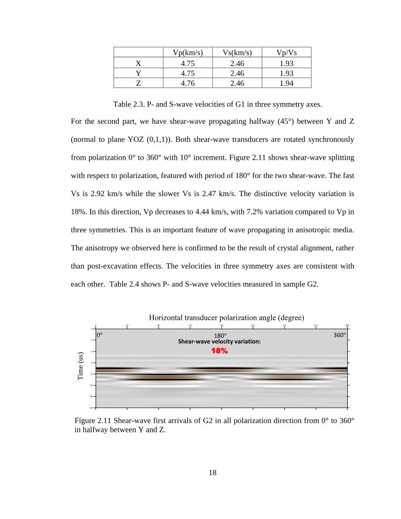
For the second part, we have shear-wave propagating halfway (45°) between Y and Z

(normal to plane YOZ (0,1,1)). Both shear-wave transducers are rotated synchronously

from polarization 0° to 360° with 10° increment. Figure 2.11 shows shear-wave splitting

with respect to polarization, featured with period of 180° for the two shear-wave. The fast

Vs is 2.92 km/s while the slower Vs is 2.47 km/s. The distinctive velocity variation is

18%. In this direction, Vp decreases to 4.44 km/s, with 7.2% variation compared to Vp in

three symmetries. This is an important feature of wave propagating in anisotropic media.

The anisotropy we observed here is confirmed to be the result of crystal alignment, rather

than post-excavation effects. The velocities in three symmetry axes are consistent with

each other. Table 2.4 shows P- and S-wave velocities measured in sample G2.

Table 2.3. P- and S-wave velocities of G1 in three symmetry axes.

Horizontal transducer polarization angle (degree)

Tim

e (u

s)

Shear-wave velocity variation:

18%

Figure 2.11 Shear-wave first arrivals of G2 in all polarization direction from 0° to 360°

in halfway between Y and Z.

180°

360°

0°

19

Vp(km/s) Vs(km/s) Vp/Vs

4.44

S1:2.92 1.52

S2:2.47 1.80

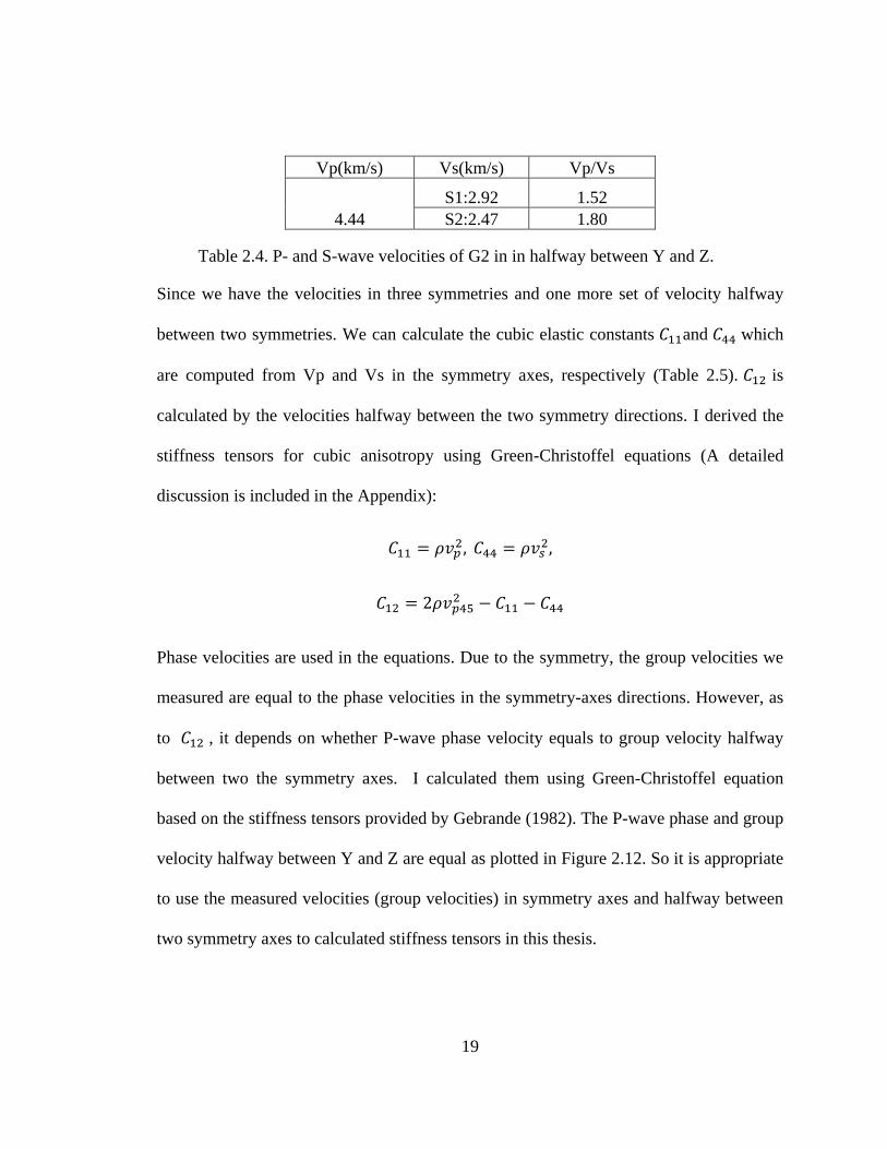
Since we have the velocities in three symmetries and one more set of velocity halfway

between two symmetries. We can calculate the cubic elastic constants 𝐶11and 𝐶44 which

are computed from Vp and Vs in the symmetry axes, respectively (Table 2.5). 𝐶12 is

calculated by the velocities halfway between the two symmetry directions. I derived the

stiffness tensors for cubic anisotropy using Green-Christoffel equations (A detailed

discussion is included in the Appendix):

𝐶11 = 𝜌𝑣𝑝2, 𝐶44 = 𝜌𝑣𝑠

2,

𝐶12 = 2𝜌𝑣𝑝452 − 𝐶11 − 𝐶44

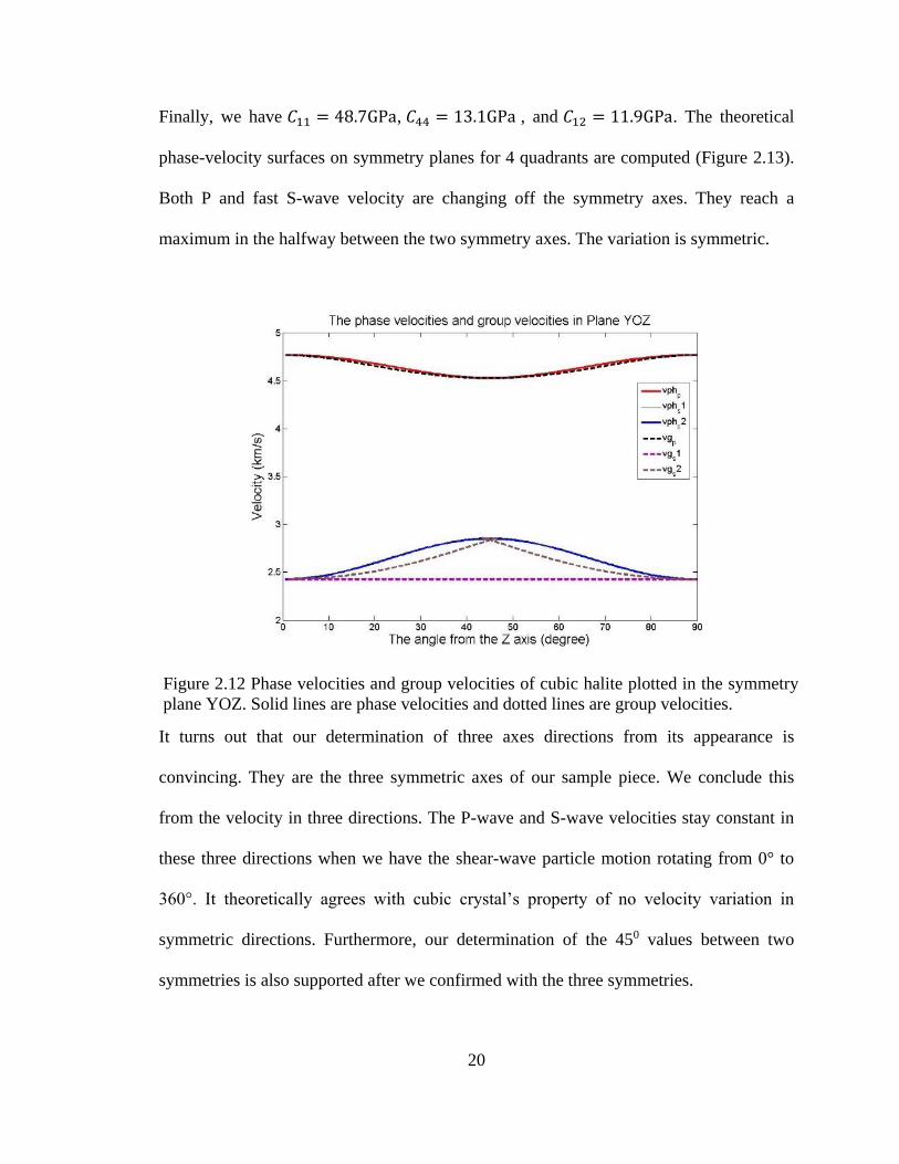
Phase velocities are used in the equations. Due to the symmetry, the group velocities we

measured are equal to the phase velocities in the symmetry-axes directions. However, as

to 𝐶12 , it depends on whether P-wave phase velocity equals to group velocity halfway

between two the symmetry axes. I calculated them using Green-Christoffel equation

based on the stiffness tensors provided by Gebrande (1982). The P-wave phase and group

velocity halfway between Y and Z are equal as plotted in Figure 2.12. So it is appropriate

to use the measured velocities (group velocities) in symmetry axes and halfway between

two symmetry axes to calculated stiffness tensors in this thesis.

Table 2.4. P- and S-wave velocities of G2 in in halfway between Y and Z.

20

Finally, we have 𝐶11 = 48.7GPa, 𝐶44 = 13.1GPa , and 𝐶12 = 11.9GPa. The theoretical

phase-velocity surfaces on symmetry planes for 4 quadrants are computed (Figure 2.13).

Both P and fast S-wave velocity are changing off the symmetry axes. They reach a

maximum in the halfway between the two symmetry axes. The variation is symmetric.

It turns out that our determination of three axes directions from its appearance is

convincing. They are the three symmetric axes of our sample piece. We conclude this

from the velocity in three directions. The P-wave and S-wave velocities stay constant in

these three directions when we have the shear-wave particle motion rotating from 0° to

360°. It theoretically agrees with cubic crystal’s property of no velocity variation in

symmetric directions. Furthermore, our determination of the 450 values between two

symmetries is also supported after we confirmed with the three symmetries.

Figure 2.12 Phase velocities and group velocities of cubic halite plotted in the symmetry

plane YOZ. Solid lines are phase velocities and dotted lines are group velocities.

21

C11 C44 C12

Cubic salt 48.7 13.1 11.9

Table 2.6 shows some previous tests on halite single crystal which give the elastic

constants.

C11 C44 C12

Zong, Dyaur 48.7 13.1 11.9

(Gebrande et al., 1982) 49.1 12.7 14.0

(Sun, 1994) 47.0 12.3 14.0

2. Salt core from Bayou Corne Salt Dome, Louisiana (L1, L2)

The experiment on L1 is a previous work conducted by Dr. Nikolay Dyaur and the Rock

Physics Lab, University of Houston. The Louisiana salt sample is cut from a 4-inch

(101.60 mm) diameter salt core. The visible granular crystal is irregular and has a size

ranged from 3 to 20 mm.

Table 2.5. Elastic constants calculated from lab measurements of pure halite.

Table 2.6. Comparison with previous measurements on halite crystal elastic constants.

P

SV

SH

Figure 2.13 Phase velocity surfaces in 4 quadrants on symmetry plane.

22

The bench-top test is carried out by Dr. Nikolay Dyaur first under room temperature and

pressure. Experimental setup is the same as what we have for salt crystal measurement.

Rotation axis is the core axis. As we see from Figure 2.14, the azimuthal compressional

and shear velocities show variance with respect to polarization. The angle between

maximum and minimum velocities for both compressional and shear-wave is around 90°.

Besides, shear-wave splitting is very clear. They are all believed to be the signs of

anisotropy.

Two sets of confining pressure tests on L1 and L2 was then undertaken with the

collaboration with the Rock Physics Lab, UH and the lab of Dr. Myers, Petroleum

Engineering, UH. The pressure is controlled from 0 to 4000 psi. We have a set of

velocities for L1 when loading the pressure and two sets of L2 for both loading and

unloading. The results of both L1 and L2 are put together on Figure 2.15 for better

comparison. The brown lines are P- and S-wave velocities (Vp1 and Vs1) of L1. The blue

and red lines are for L2 during loading (Vp2up and Vs2up) and unloading pressures

(Vp2down and Vs2down). The velocities under confining pressure from 0 to 4000 psi vary

from 4.4 to 4.8 km/s for P-waves and 2.5 to 2.8 km/s for the S-waves. In general, both P-

4.2

4.4

4.60

30

60

90

120

150

180

210

240

270

300

330

4.2

4.4

4.6

Vp1 av

2.4

2.5

2.6

2.70

30

60

90

120

150

180

210

240

270

300

330

2.4

2.5

2.6

2.7

Vs

1.60

1.65

1.70

0 1020

30

40

50

60

70

80

90

100

110

120

130

140

150160

170180190200

210

220

230

240

250

260

270

280

290

300

310

320

330340

350

1.60

1.65

1.70

1.75

Vp/Vs2

Figure 2.14 Azimuthal velocities of P- and S-waves in one cross section of L1. From left

to right: P-wave velocity, S-wave velocity and Vp/Vs.

23

wave and S-wave velocity increase with pressure for the two samples. The increment

slows down with the further compression. While downloading pressure for L2, the

velocity will not go back to normal, but be higher than the value while loading.

For further investigation of the reason, we carried out the CT scanning over the sample

L2 both before and after confining pressure test. Slight fractures are visible before the

confining pressure test. These fractures are randomly distributed as shown in Figure 2.16.

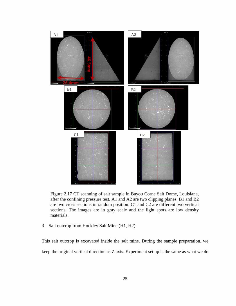
The 4000 psi confining pressure closes almost all the micro-cracks (Figure 2.17). In this

case, the micro-cracks closing during high pressure test give us a reasonable main factor

for such a velocity increment. The limitation of test device is that diameter of sample is

restricted to 1.5 inch (38 mm) maximum. Taking the size of granular crystal of this salt

Figure 2.15 Vp and Vs lab measurements under confining pressure on L1 and L2. The

brown lines are P- and S-velocities (Vp1 and Vs1) of L1. The blue and red lines are for

L2 during loading (Vp2up and Vs2up) and unloading pressures (Vp2down and Vs2down).

P-wave velocity vs. pressure

S-wave velocity vs. pressure

24

core into consideration, the small-scale velocities might not be representative for the

whole salt sample. But we still could quantify the velocity change due to pressure.

A A

B1 B2

C1 C2 D1 D2

Figure 2.16 CT scanning of salt sample in Bayou Corne Salt Dome, Louisiana, before

the confining pressure test. A1 and A2 are two clipping planes. B1 and B2 are two

cross sections in random position. C1 and C2 are different two vertical sections. D1

and D2 are 3D view of the fractures inside sample L1 from two different directions.

The images are in gray scale and the light spots are low density materials.

26.4mm

46

.5m

m

25

3. Salt outcrop from Hockley Salt Mine (H1, H2)

This salt outcrop is excavated inside the salt mine. During the sample preparation, we

keep the original vertical direction as Z axis. Experiment set up is the same as what we do

C2 C1

A1 A2

B1 B2

Figure 2.17 CT scanning of salt sample in Bayou Corne Salt Dome, Louisiana,

after the confining pressure test. A1 and A2 are two clipping planes. B1 and B2

are two cross sections in random position. C1 and C2 are different two vertical

sections. The images are in gray scale and the light spots are low density

materials.

26.4mm

46

.5m

m

26

for salt crystal measurement. We measure velocities in three axis by keeping both

transducers parallel and then rotating from polarization 0° to 360° with 10° increment.

For H1, as we can see from Figure 2.18, velocity variation is repeatable along the Y and

Z direction which is a sign of anisotropy. The velocities of both P- and S-wave are

calculated from the first arrival picks (Table 2.7). However, we are not sure about the

influence of post-excavation induced fractures. If we look at the P-wave velocities in X,

Y, and Z directions, they show that the average velocity in vertical direction Z is smaller,

while velocities in other two directions are higher. The shear-wave shows obvious

splitting in Z direction. The splitting is also shown but not very clear and easy to pick in

other two directions. Although we can still see the energy (amplitude) of fast shear-wave

decreases around 900 and 2700 in X direction and 00 and 1800 in Y direction with the

corresponding slow shear-wave energy increasing. We cannot see clear ‘splitting’ in the

waveform. When I change the shear-wave particle motion direction by rotating the

transducers, the fractures inside sample change the shear-wave energy distribution in the

two orthorhombic shear-wave directions. This inconsistence energy distribution for one

type of shear-wave suggests the anisotropy of sample. On the other hand, the P-wave

travels slowest in the Y direction. It suggests that the preferred fracture trend in this small

piece is possible to be more parallel to XOZ plane and more vertical to Y direction.

27

H1 Length

(mm)

Vp average

(km/s)

Vp STD Vs1 (km/s) Vs2 (km/s) Vs variation

(%)

X 81.27 3.96 0.22 2.44 2.16 13

Y 76.30 3.73 0.29 2.95 2.62 13

Z 60.55 4.42 0.07 2.06 1.88 10

Results of H2 (Table 2.8) are quite different from H1 in terms of the absolute value. P-

and S-wave velocities variations are still obvious. It is also clear that velocities in H2 are

higher than those in H1. However, the two samples show consistence with each other in

three axes that the slowest P-wave velocity happens in Y direction. P-wave velocities in

X and Y direction vary in much larger scale than in Z direction (standard deviation values

Z

Y

X Z

Y

X Z

Y

X

Tim

e (u

s)

Horizontal transducer polarization angle (degree)

Figure 2.18 Shear-wave first arrivals of H1 in all polarization direction from 0° to 360°.

From top to bottom: shear-wave records in X, Y and Z directions.

Table 2.7 P- and S-wave velocities of H1 calculated from first arrivals.

180°

180°

360°

Figu

re 2.

10

Shea

r-

wave

first

arriv

als of

H3

in all

polar

izatio

n

direc

tion

from

0° to

360°.

From

top

to

botto

m:

shear

-

wave

recor

ds in

X, Y

and

Z

direc

tions.

360°

0°

0°

X

X

Y

X

Z

X

28

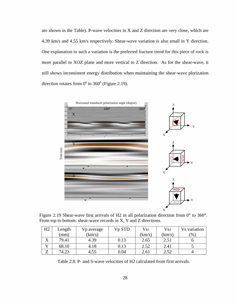
are shown in the Table). P-wave velocities in X and Z direction are very close, which are

4.39 km/s and 4.55 km/s respectively. Shear-wave variation is also small in Y direction.

One explanation to such a variation is the preferred fracture trend for this piece of rock is

more parallel to XOZ plane and more vertical to Z direction. As for the shear-wave, it

still shows inconsistent energy distribution when maintaining the shear-wave plorization

direction rotates from 00 to 3600 (Figure 2.19).

H2 Length

(mm)

Vp average

(km/s)

Vp STD Vs1

(km/s)

Vs2

(km/s)

Vs variation

(%)

X 79.41 4.39 0.13 2.65 2.51 6

Y 68.10 4.18 0.13 2.52 2.41 5

Z 74.23 4.55 0.04 2.61 2.52 4

Table 2.8. P- and S-wave velocities of H2 calculated from first arrivals.

Y

X

Z

Z

Y

X

Z

Y

X

X

Y

Z

Tim

e (u

s)

Horizontal transducer polarization angle (degree)

0°

180°

360°

Figure 2.19 Shear-wave first arrivals of H2 in all polarization direction from 0° to 360°.

From top to bottom: shear-wave records in X, Y and Z directions.

29

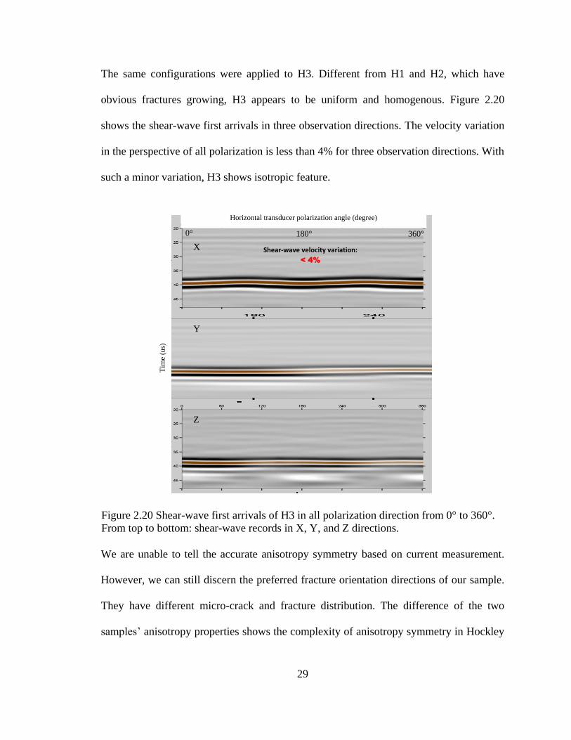
The same configurations were applied to H3. Different from H1 and H2, which have

obvious fractures growing, H3 appears to be uniform and homogenous. Figure 2.20

shows the shear-wave first arrivals in three observation directions. The velocity variation

in the perspective of all polarization is less than 4% for three observation directions. With

such a minor variation, H3 shows isotropic feature.

We are unable to tell the accurate anisotropy symmetry based on current measurement.

However, we can still discern the preferred fracture orientation directions of our sample.

They have different micro-crack and fracture distribution. The difference of the two

samples’ anisotropy properties shows the complexity of anisotropy symmetry in Hockley

Tim

e (u

s)

Horizontal transducer polarization angle (degree)

Shear-wave velocity variation:

< 4%

Figure 2.20 Shear-wave first arrivals of H3 in all polarization direction from 0° to 360°.

From top to bottom: shear-wave records in X, Y, and Z directions.

0°

180°

180°

180°

360°

180°

X

X

Y

X

Z

X

30

Salt Mine. On the other hand, sample size is so small that it only shows the local fracture

trend. Only with large amount of measurements in different region that could we tell

something about the global dominant stress orientation. Further experiments under high

pressure are needed to confirm effects of arbitrary external fractures.

4. Salt cores from Hockley Salt Mine (H4, H5)

The two salt cores (H4 and H5) are cut from different horizontal wells, 4-inches (101.6

mm) diameter. The original horizontal direction is known but not the vertical one. Since

we are not aware of the preferred fracture direction, we measure the azimuthal velocity

from three different sections of salt cores and non-zero source-receiver offset for a better

exploration of the possible orientation direction.

The zero-offset measurements are finished in three sections (a, b, c) of each sample with

a distance of 30 mm. Shear-wave source and receiver transducers are put parallel to each

other in the opposite sides of core sample. During the measurement, we keep the

transducers parallel and fixed. Then we rotate the core from polarization 0° to 360° with

10° increment. In this case, we observe the velocity variation when shear-wave travels

through the cross section at section a. Meanwhile, we can also observe the P-wave from

the oscilloscope monitor due to the shear-wave energy dispersion and conversion to P-

wave during traveling.

31

From different sections of H4 and H5, both P- and S-wave variations are observed with

all polarization directions. The variation are quite small compared with those in other

samples. The standard deviation for both P- and S-wave velocities ranges from 0.02 to

0.04 km/s, which are less than 1%. There is no obvious shear-wave splitting in any

sections (Figure 2.21). The variation happens periodically so that I show the value by

averaging the two values with 180° angular difference. In the same section, the P-and S-

wave velocity variation shows uniformity. However, there is no unified orientation when

we look at the three sections in one core. The core axis is not the direction of maximum

anisotropy. We cannot generate a dominant symmetry from the zero-offset results for this

Horizontal transducer polarization angle (degree)

Tim

e (u

s)

Figure 2.21 Shear-wave first arrivals of H4 and H5 in all polarization direction from 0°

to 360°. From top to bottom: shear-wave records in X, Y, and Z directions.

H4 H5

32

core.

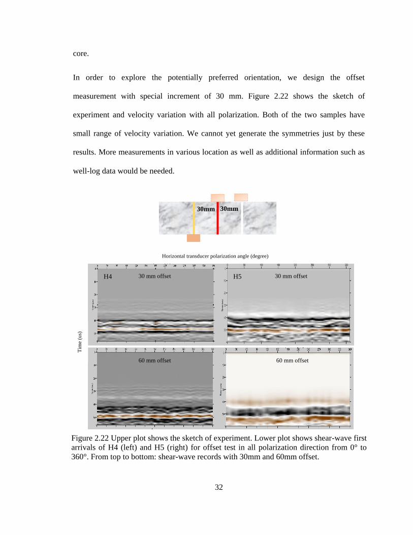
In order to explore the potentially preferred orientation, we design the offset

measurement with special increment of 30 mm. Figure 2.22 shows the sketch of

experiment and velocity variation with all polarization. Both of the two samples have

small range of velocity variation. We cannot yet generate the symmetries just by these

results. More measurements in various location as well as additional information such as

well-log data would be needed.

Horizontal transducer polarization angle (degree)

Tim

e (u

s)

30mm

30mm

Figure 2.22 Upper plot shows the sketch of experiment. Lower plot shows shear-wave first

arrivals of H4 (left) and H5 (right) for offset test in all polarization direction from 0° to

360°. From top to bottom: shear-wave records with 30mm and 60mm offset.

30 mm offset 30 mm offset

60 mm offset 60 mm offset

H4 H5

33

2.5 Discussion

The measurements over pure halite sample from Goderich, Ontario were undertaken first

in the lab. The data indicates the cubic anisotropy properties as the previous work done

with the pure salt. What is more, according to our measurements for velocity variation

half-way between two symmetries (7% and 18% for Vp and Vs respectively), the

difference caused by cubic symmetry is not ignorable. I build a salt model with the

calculated stiffness tensors applied to quantify such difference in field scale. It could be

the reference for those area with thick pure salt formations. However, due to the

limitations of laboratory sample preparation and measurement instruments, I have not

included the velocity measurements in other directions in my thesis. The current results

are carried out in the most essential directions that could help to calculate the elastic

constants and anisotropy parameters. Theoretical velocity distribution as well as

traveltimes could be calculated from the moduli. Measurements with full azimuthal

polarization under high pressure is preferred for a strict and precise illumination for cubic

anisotropy.

Tectonically speaking, the main processes shape the salt structures in the Gulf of Mexico

area is divided into two parts: those make the Gulf deeper (original salt deposition) and

those make it shallower (later salt flowage). The dominant stresses have the major

influence on the alignment of salt basin (Balk, 1953).

34

The main salt accumulation in the Gulf of Mexico area occurred in the Jurassic when the

granite core of the North American tectonic plate began to separate from South America

and Africa over 100 million years ago; this began the formation of the Gulf of Mexico.

All the structural and stratigraphic features seen today were in place since then. The

initial breakup of Pangea in the Early Jurassic led to the formation of grabens and half-

grabens which became the location for the earliest sediments deposited in the Gulf of

Mexico. Initially these grabens that were offshore Texas and Louisiana filled with red

beds. After red bed deposition, marine conditions began to characterize the northern Gulf

of Mexico in the Middle Jurassic time. This caused the widespread deposition of

evaporites typically referred to as the Louann Salt sheet (Salvador, 1991). There is

document about the mode of origin as well as the crystal deformation and

recrystallization in salt domes in Louisiana, TX (Balk, 1953).

Over millions of years, plumes of the light salt began to float up through the heavier

sediment that covered it. As the salt made it very close to the surface, sometimes having

traveled through more than 10 km of rock and sediment, it pushed up the sea floor above

it to form a mound or dome. During the flowing, the salt crystals were aligned in the

flowage direction and recrystallized. It is reported that salt layers stand vertically, or

nearly so. The mine exposures approach the southeastern border of the dome and strike

parallel with it. The common occurrence of distorted halite crystal and preferential

orientation of longest body axis of anhydrite crystal suggests the vertical lineation of

dominant stresses direction happened in Louisiana salt dome. Balk (1953) compares two

salt domes in Louisiana to show their similarity in the salt origin and the preferred

35

orientation of crustal alignment. It gives the reference for the investigation of dominant

salt structures orientation in close terrain in the Gulf Coast area.

The Hockley Salt Mine is one typical salt dome in the Gulf Coast. Based on the study of

the shape and internal structure through the deformation and recrystallization of an

essentially dry crystal aggregate under a shear stress, We expect to see the influence of

dominant stresses during the formation of broad salt basin in the Gulf Coast from the

velocity. If it has the same prevailingly vertical crystal orientation, the anisotropy

symmetry is close to VTI model. Our salt blocks from the Hockley Salt Mine show

significant anisotropy but with different orientation directions. This could be for a

number of reasons. First of all, our samples are taken from a stressed zone. During the

excavation, the shear stress could be released and meanwhile produce fractures by

external force. Secondly, the sample size is too small for giving a representative view for

global trend. Limited number of small-sized samples could provide the microscope

information of local trend. We still need large amount of sample in different area to get

statistical results for generating the dominant stress orientation.

Even though we cannot conclude the preferred orientation or accurate symmetry for

Hockley Salt Mine from current samples, the significant anisotropy properties are shown

with both shear-wave splitting and P-wave velocity variation in some directions.

Comparing our results in salt cores and blocks, the salt cores with horizontal core axis do

show minor P- and S-wave velocity variation when we maintain the shear-wave

propagating parallel to the vertical plane. But such slight variation could not support its

36

anisotropy type. It appears more like an isotropic medium. All the measurements we have

done are provided for reference.

Generally speaking, two kinds of salt samples show significant anisotropy properties

from the lab measurements. The pure halite salt and the fractured salt with preferred

fracture orientation. It suggests two scenarios where we might need to pay attention when

building velocity models. One is the formation with large pure and undeformed salt

deposition, such as North Wilson Basin and Michigan Basin. In this situation, cubic

symmetry is expected to show up. Another is the salt structures with dominant stresses

and have orientated fractures developed. The anisotropic symmetry depends on the

orientation of fractures for this case.

37

Chapter 3

Empirical relationships of salt in the Gulf of Mexico coast from well-log

data

3.1 Introduction

Geophysical well-log measurements provide important information of the rocks that they

traverse. This includes: the physical properties of the rock framework, the fluid in the

formation, and the environmental state in the subsurface of the borehole (fluid and

rugosity). Log values can depend on the volume of the rock investigated by the probe, the

vertical resolution of the probe (thin-bed resolution), and the design characteristics of

each individual logging tool (Daniels et al., 1980). As one of the most direct way to

obtain geophysical values, the log measurements are often regarded as ‘ground truth

versus the remote sensing imagery.

In this chapter, I investigate 142 wells drilled through salt to extend my study of salt

geophysical properties from lab salt samples to salt structures in the Gulf of Mexico area.

With the wide spread of these wells in the Gulf of Mexico area, I generate the empirical

relationships of salt velocity with depth and density from the statistical data. And then

further predict the velocity with pressure from depth. These relationships could provide a

reference for building salt velocity model. Density, sonic and gamma logs are studied. All

the well data are provided by Dr. Fred Hilterman and Geokinetics. The well data are

processed with Geoview software of Hampson-Russell package and Matlab software.

38

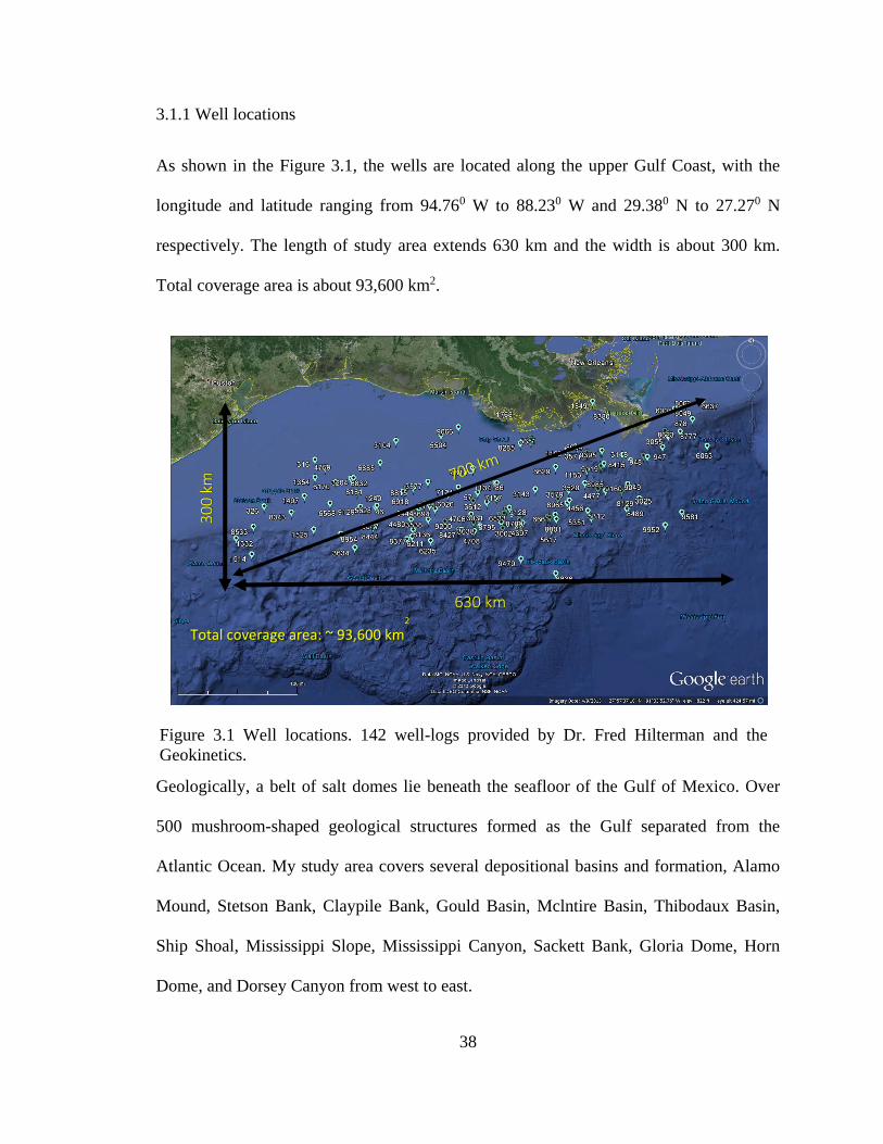
3.1.1 Well locations

As shown in the Figure 3.1, the wells are located along the upper Gulf Coast, with the

longitude and latitude ranging from 94.760 W to 88.230 W and 29.380 N to 27.270 N

respectively. The length of study area extends 630 km and the width is about 300 km.

Total coverage area is about 93,600 km2.

Geologically, a belt of salt domes lie beneath the seafloor of the Gulf of Mexico. Over

500 mushroom-shaped geological structures formed as the Gulf separated from the

Atlantic Ocean. My study area covers several depositional basins and formation, Alamo

Mound, Stetson Bank, Claypile Bank, Gould Basin, Mclntire Basin, Thibodaux Basin,

Ship Shoal, Mississippi Slope, Mississippi Canyon, Sackett Bank, Gloria Dome, Horn

Dome, and Dorsey Canyon from west to east.

30

0 k

m

630 km

Total coverage area: ~ 93,600 km2

Figure 3.1 Well locations. 142 well-logs provided by Dr. Fred Hilterman and the

Geokinetics.

39

The largest salt structure appears in this study area is the Sigsbee salt canopy (Figure 3.2),

which is also the largest known salt structure on Earth. This canopy comprises more than

100 salt sheets and stocks that coalesced to cover more than 137,000 km2 on the lower

continental slope of the northern Gulf of Mexico (Hudec and Jackson, 2009). The

southwest part of my study area covers the Sigsbee salt canopy.

Figure 3.21 (A) Map of the northern Gulf of Mexico showing location of the Sigsbee salt

canopy. (B) Map of the Sigsbee salt canopy, showing peripheral thrust systems (thick

lines with triangles) and approximate extent of submarine fans. Outline of the Sigsbee

salt canopy is based on the mapping and bathymetric data from Bryant and Liu (2000).

Fan outlines interpreted from bathymetric contours in Taylor et al. (2002). Named

polygonal blocks are Minerals Management Service protraction areas. (Hudec and

Jackson, 2009)

40

The study area is pronounced by its high production of energy resources. It is near the

heart of U.S. petrochemical industry and also one of the most developed oil and gas

industries in the world. As the salt domes are widely distributed and are important

structures in the Gulf Coast, my study tries to provide a general reference for the salt

properties.

3.1.2 Salt identification on well-logs

By combining various log parameters, salt formation could be distinguished from other

deposits such as sandstones, limestone, dolomites and so on.

Following are the salt identifications showing in different logs:

a. Gamma ray

Gamma ray log measurements are natural gamma ray emission from radioactive

formations. The principal natural gamma-ray emitting minerals in the evaporite sequence

are uranium, potassium-40 and thorium.

Halite has a nearly zero gamma-ray response, also does anhydrite and dolomite. On the

other hand, Potash minerals have very high gamma-ray responses: 200 API units for

carnallite but possibly over 700 API units for sylvite (Crain, 1986). Shale has an

intermediate to high gamma-ray response. The gamma ray log is a good indicator of

potash.

41

b. Density

The density probe consists of a gamma-ray source and one or more gamma-ray detectors.

Gamma rays emitted by the source are scattered by the rock formation as an inverse

function of the electron density of the rocks (Daniels, Hite, and Scott, 1980).

The apparent electron density of halite is 2.04 to 2.07 g/cm3 in the Gulf Coast according

to the log data. The densities of the cap rock and embedded deposits such as limestone

(around 2.37 g/cm3), anhydrite (around 2.98 g/cm3) are higher while those of the potash

minerals (carnallite and sylvite) are lower (less than 2.0 g/cm3). Unlike other sedimentary

rocks which have bulk density generally the same as the density log readings, the salt

bulk density (around 2.16 g/cm3) usually does not match well with the measurements

(Gilreath, 1983). Corrections are necessary for a more accurate measurement.

For other sedimentary rocks, Daniels et al. (1980) recorded that the clay and shale have

low apparent bulk densities (2.2 to 2.6 g/cm3), sandstone has intermediate apparent bulk

densities (2.45 to 2.65 g/cm3), and dolomite has a high apparent bulk density (2.7 to 2.9

g/cm3) in three drill holes at Salt Valley, Utah.

c. Resistivity

Resistivity is the reciprocal of conductivity. The electrical conductivity is controlled by

the nature, quantity and distribution of the water contained in the bed. The resistivity of

consolidated halite is generally greater than 10,000 ohm-m, which contrasts markedly

with the resistivity of the cap rock and interbed (Daniels, Hite, and Scott, 1980). The

extremely high resistivity (low conductivity) of halite comes from its crystal structure.

42

The sodium and chlorine ions are locked in the cubic lattice so that they could not travel

through the formation as they do when dissolved in water.

The resistivity log used here jump to the maximum value in salt layers which make salt

easily distinguished from other lithologies. It helps to locate the salt top as well as bottom.

While the value is not applicable since it always reaches the upper limit. However, the

resistivity response itself could not be considered as a unique salt signature since other

formation such as cap rock, sulphur, highly cemented sand as well as sands having low

water saturation also exhibit high values.

d. Neutron

The number of neutrons counted at the receiver is inversely proportional to the hydrogen

content of the rocks surrounding the borehole, and is primarily a measure of the amount

of water and hydrocarbons contained in the rocks. The neutron porosity of halite and

anhydrite is low due to the low hydrogen content and high density. It is extremely high in

gypsum due to the high hydrogen during the recrystallization. It is intermediate in

sandstone and dolomite, and low in carnallite and black shale. However, dense sandstone,

limestone and sulphur can also have similar response as halite due to the low porosity

(Gilreath, 1983).

e. Acoustic velocity

The sonic log is a porosity log that measures interval transit time of a compressional

sound wave traveling through one foot of formation. It is dependent upon both lithology

and porosity (Gilreath, 1983).

43

The acoustic velocity is high for carnallite, anhydrite, and dolomite (approximately 5000

m/s), intermediate for halite (approximately 4500 m/s), and low for gypsum and shale

(approximately 3000 m/s) (Daniels, Hite, and Scott, 1980).

f. Caliper

The caliper log gives a continuous measurement of size and shape of a borehole along its

depth. It is another recognizable factor for salt. Because some salt deposits are quite

soluble in water-based drilling fluids and resulting for the enlargement of borehole

(Tixier and Alger, 1970). It is often used by combining with other logs such as the

resistivity for better verification (Lishman, 1961). Caliper response also makes it possible

to separate some evaporite mineral from clean salt such as anhydrite.

Generally, it is not reliable to separate the salt from other sedimentary rocks based on a

single log value. It is essential to combining different logs for the determination. Salt

deposits are typically non-radioactive, non-porous, low density, high velocity, electrically

nonconductive and soluble. They are highly recognizable in the logging records with high

sonic velocity, extremely high resistivity. Resistivity is a good delineator of the top and

bottom. The caliper log is also a good indicator especially when combined with resistivity

logs. The sonic and density or neutron logs usually will provide more identifiable

information of the evaporite minerals. Table 3.1 shows the lithology information (Hite

and Lohman, 1973) and physical properties (Tixier and Alger, 1970) of salt formation in

GoM. The salt formation in my thesis is defined from the records of the top of salt.

44

Specific

Gravity (g/cm3)

Log Density

(g/cm3)

Velocity

(km/s)

Natural

Radioactivity

Water Content

Halite 2.16 2.032 4.4-6.5 None Very Low

Sylvite 1.99 1.863 4.6-6.5 High Low

Anhydrite 2.96 2.977 4.1 None Very Low

Carnallite 1.61 1.570 4.4-6.5 Low High

Dolomite 2.87 2.683 3.5-6.9 None Low

Gypsum 2.32 2.351 2-3.5 None Intermediate

Shale 2.2-2.6 2.2-2.75 2.3-4.7 High Intermediate-High

3.2 Salt velocity versus depth

The precise seismic velocity depends upon the mineral composition and the granular

nature of the rock matrix, cementation, porosity, fluid content, and environmental

pressure. Depth of burial and geologic age also have an effect (Gardner et al., 1974).

Depth of burial leads to temperature and pressure increase. Temperature tends to decrease

the speed of seismic waves and pressure tends to increase the speed. Pressure increases

with depth in Earth because the weight of the rocks above gets larger with increasing

depth. Usually, the effect of pressure is the larger and in regions of uniform composition,

the velocity generally increases with depth, despite the fact that the increase of

temperature with depth works to lower the wave velocity. Normally, the lab

measurements could often be operated under high pressure or temperature. While it is

impossible to carry that out with depth under control. The investigation of the

relationship between salt velocity and depth in this chapter is trying to give a reference

for better velocity model building.

The salt studied in this chapter has different types of structures according to the well-log

data. Some of the wells were drilled through salt formation where we could have a clear

Table 3.1. Lithology information and physical properties of salt formation in the Gulf of

Mexico (After Tixier and Alger, 1970 and Hite and Lohman, 1973).

45

view of the thickness. There are also small amount of wells did not continue very far after

they reached the top of salt where we just don’t have the bottom of salt. The depth data of

these 142 wells in this chapter has a large range from 1.5 km to 6.5 km, with most data

concentrated in 2.5 km to 4 km. The thickest salt formation is up to 2.23 km (7300 ft),

occurs in the depth of 3.75 to 5.97 km (12300 to 19600 ft), located at 27°49'5.98"N,

88°55'12.16"W.

With such a huge data volume from this large coverage, it was not possible to analyze

each log in this thesis. We do not investigate the detail salt structure type for each log in

this chapter. General data of velocity and depth are read directly from sonic log and true

vertical depth. Top of the salt distribution is plot in Figure in perspective of well location.

From this distribution, we could find that the occurrence of salt structures could be very

different - from 1370 to 6130 m (4500 to20100 ft).

According to the reports of Sigsbee salt canopy (Hudec and Jackson, 2009), for the major

salt structure in my study area, the top of salt canopy is around 2500m. It agrees with our

readings of the southwest part. The shallower readings are possibly the salt-roof trust

while the very deep readings are possibly the base salt. With limited knowledge of all the

salt structures within my study area and the randomly distributed dataset, it is not

applicable to separate these data set by different structure type. Basically, we cannot see

obvious or large uniformed salt structures distribution trend from current dataset.

However, it is not reasonable to conclude that the salt structures are well developed and

of high complexity in the Gulf of Mexico coast.

46

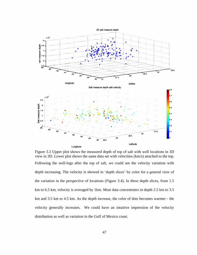
The top of salt just provides the occurrence of salt. Figure 3.3 shows the readings of

velocity of the salt tops in different locations from sonic log. By attaching the velocity to

the salt, we see a variation that ranges from 4.1 to 4.8 km/s of the top of salt. The

dominant velocity of salt top is from 4.3 to 4.5 km/s. Such range of variation could be

generated from different structure types and different evaporites mineral compositions

such as low velocity gypsum which often appears in cap rock.

47

Following the well-logs after the top of salt, we could see the velocity variation with

depth increasing. The velocity is showed in ‘depth slices’ by color for a general view of

the variation in the perspective of locations (Figure 3.4). In these depth slices, from 1.5

km to 6.5 km, velocity is averaged by 1km. Most data concentrates in depth 2.5 km to 3.5

km and 3.5 km to 4.5 km. As the depth increase, the color of dots becomes warmer - the

velocity generally increases. We could have an intuitive impression of the velocity

distribution as well as variation in the Gulf of Mexico coast.

Figure 3.3 Upper plot shows the measured depth of top of salt with well locations in 3D

view in 3D. Lower plot shows the same data set with velocities (km/s) attached to the top.

48

Figure 3.4 Average velocity (km/s) in different depth (km) with respective to well location.

49

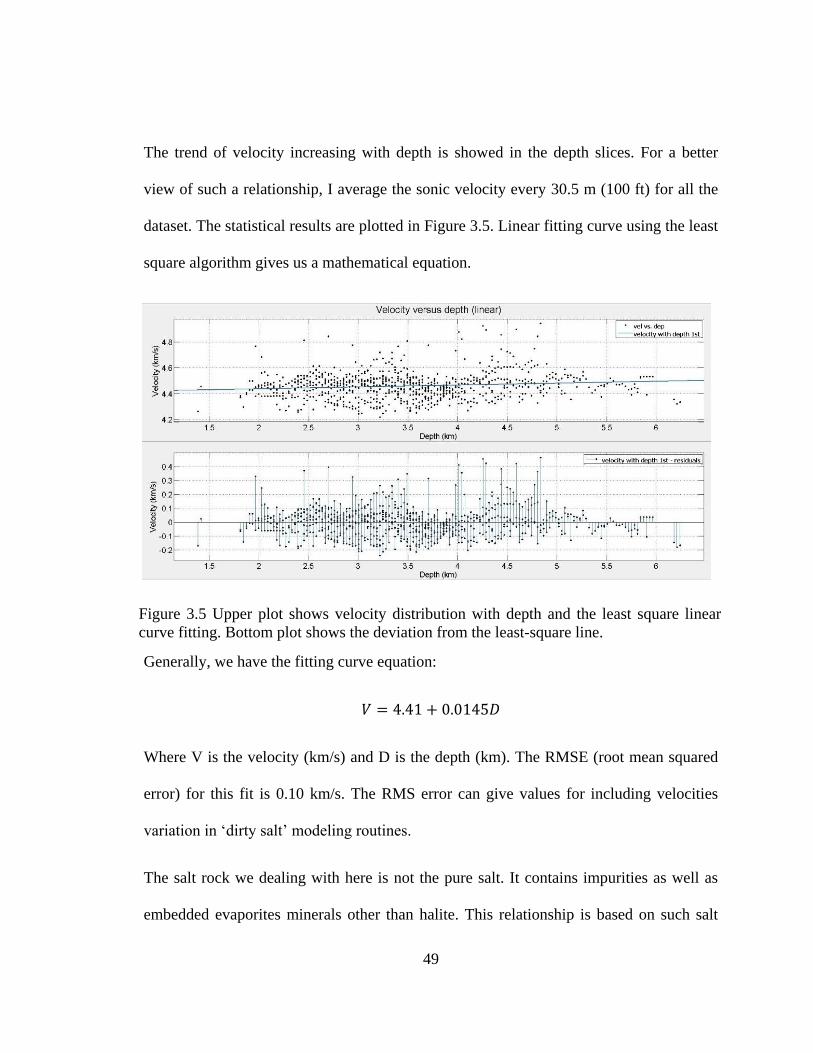
The trend of velocity increasing with depth is showed in the depth slices. For a better

view of such a relationship, I average the sonic velocity every 30.5 m (100 ft) for all the

dataset. The statistical results are plotted in Figure 3.5. Linear fitting curve using the least

square algorithm gives us a mathematical equation.

Generally, we have the fitting curve equation:

𝑉 = 4.41 + 0.0145𝐷

Where V is the velocity (km/s) and D is the depth (km). The RMSE (root mean squared

error) for this fit is 0.10 km/s. The RMS error can give values for including velocities

variation in ‘dirty salt’ modeling routines.

The salt rock we dealing with here is not the pure salt. It contains impurities as well as

embedded evaporites minerals other than halite. This relationship is based on such salt

Figure 3.5 Upper plot shows velocity distribution with depth and the least square linear

curve fitting. Bottom plot shows the deviation from the least-square line.

50

rock without improving the data quality by separating the other minerals. The intention of

doing so is to provide a more realistic reference for salt velocity model in the Gulf of

Mexico. The original data is representative for salt formation in the Gulf of Mexico.

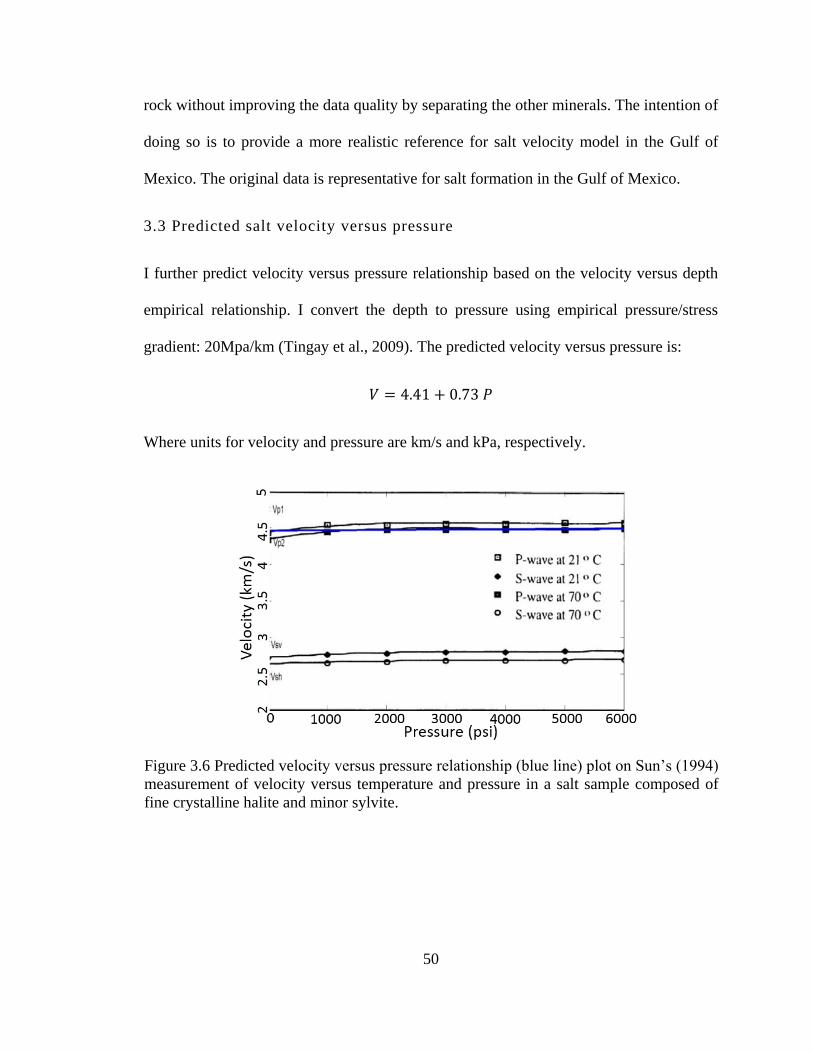
3.3 Predicted salt velocity versus pressure

I further predict velocity versus pressure relationship based on the velocity versus depth

empirical relationship. I convert the depth to pressure using empirical pressure/stress

gradient: 20Mpa/km (Tingay et al., 2009). The predicted velocity versus pressure is:

𝑉 = 4.41 + 0.73 𝑃

Where units for velocity and pressure are km/s and kPa, respectively.

Figure 3.6 Predicted velocity versus pressure relationship (blue line) plot on Sun’s (1994)

measurement of velocity versus temperature and pressure in a salt sample composed of

fine crystalline halite and minor sylvite.

51

I correlate this predicted relationship to other measurements in the literature for both lab

and field. Figure 3.6 shows the comparison with Sun’s (1994) measurements for a salt

sample composed of fine crystalline halite and minor sylvite. The predicted relationship

(blue line) fits Sun’s measurement at 70oC. The geothermal gradients is about 25 oC per

km of depth in most of the world (Tingay, Hillis, Morley, King, Swarbrick and Damit,

2009). Since most logging data is concentrated at 2.5km to 3.5km, the dominant

temperature is 60 to 80 oC as well. Another comparison is to the field data of the

Pripyatskaya Depression, Russia (Volarovich et al., 1986). Figure 3.7 shows velocity

versus pressure for different lithology. Our predicted relationship (red line) is located at

the upper bound of Volarovich’s record of salt (halite). The coherence to both lab

measurement and field data from previous study suggests applicability of the empirical

relationship of velocity and depth.

Pressure

Ve

lo

Salt (Halite)

Figure 3.7 The predicted velocity versus pressure relationship (red line) plot on

Volarovich’s field measurements of the Pripyatskaya Depression, Russia.

52

3.4 Salt velocity versus density

Lithology and porosity can be related empirically to velocity by the time-average

equation. This equation is most reliable when the rock is under substantial pressure and,

saturated with brine, as well as contains well-cemented grains (Gardner, Gardner and

Gregory, 1974). The electron velocity reading for salt is not true bulk density. However,

the empirical correlation of density and velocity from field measurements are satisfactory

applicable for particular formations and environments, which, in this chapter, the Gulf of

Mexico. As recorded by Lines (2004), salt is unusual in that it does not follow the normal

seismic velocity-density relationships of many other rocks (Lines and Newrick, 2004).

Gardner also gave a sketch of rock salt in his velocity-density relationship.

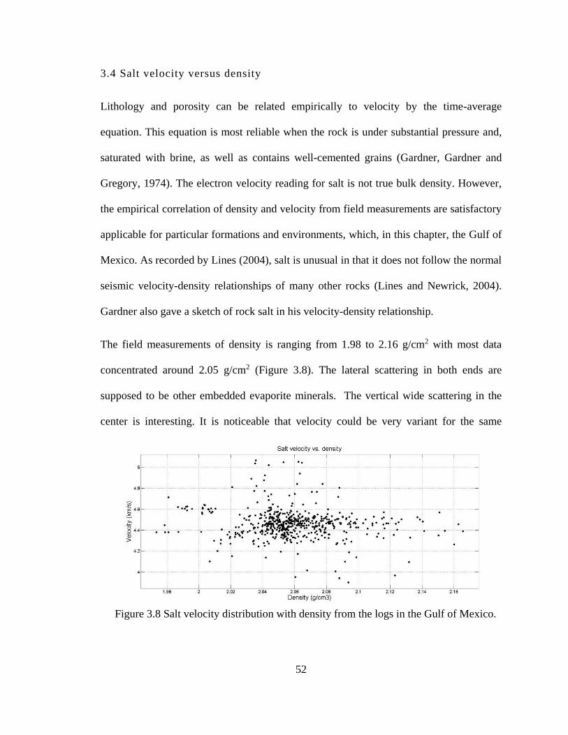
The field measurements of density is ranging from 1.98 to 2.16 g/cm2 with most data

concentrated around 2.05 g/cm2 (Figure 3.8). The lateral scattering in both ends are

supposed to be other embedded evaporite minerals. The vertical wide scattering in the

center is interesting. It is noticeable that velocity could be very variant for the same

Figure 3.8 Salt velocity distribution with density from the logs in the Gulf of Mexico.

53

density. There are many possible explanations for such variation. The different crystal or

fracture orientation along the borehole could be one reason for various sonic log readings,

even though the orientation does not affect the density. But before precise analysis to the

composition as well as fractures, no valid conclusion could be generated.

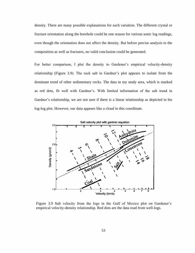
For better comparison, I plot the density to Gardener’s empirical velocity-density

relationship (Figure 3.9). The rock salt in Gardner’s plot appears to isolate from the

dominant trend of other sedimentary rocks. The data in my study area, which is marked

as red dots, fit well with Gardner’s. With limited information of the salt trend in

Gardner’s relationship, we are not sure if there is a linear relationship as depicted in his

log-log plot. However, our data appears like a cloud in this coordinate.

Figure 3.9 Salt velocity from the logs in the Gulf of Mexico plot on Gardener’s

empirical velocity-density relationship. Red dots are the data read from well-logs.

54

3.5 Discussion

Compared with lab measurements, the field measurements provide a more realistic

reference for building velocity model in specific environment with multiple influencing

factors and other unknowns entailed (Gardner, Gardner, and Gregory, 1974).

The general relationship of salt velocity and depth is generated with a linear least square

curve fitting. Basically velocity increases slightly with depth. The density of rock salt

does not show clear relationship with velocity.

55

Chapter 4

Numerical modelling of salt

4.1 Introduction

Our lab measurements of pure salt are consistent with pure halite crystals, showing cubic

symmetry. Anisotropy parameters are calculated in Chapter 2 as 𝐶11 = 48.7𝐺𝑃𝑎, 𝐶44 =

13.1𝐺𝑃𝑎 , and 𝐶12 = 11.9𝐺𝑃𝑎. In this chapter, numerical models are built to investigate

the travel time differences caused by cubic anisotropy.

4.2 Phase and group velocities distribution in space

For the cubic anisotropic media, we have three independent elastic

constants:𝐶11, 𝐶44 , 𝐶12 . Phase velocities, and group velocities could be calculated by

using first and second Green Christoffel equations:

ljijklik nnC

02 kikik UVph

kiijkljl UUC

ljl

ph

g

j nVk

V

1

56

Based on the elastic constants we calculated from lab measurements through pure halite

samples in Chapter 2, we could get the phase and group velocities. As shown in Figure

4.1, we calculated the velocity distribution in space. The results show eighth of the space

when we have ϴ and φ varying from 0 to π/2. The color represents for the value of

velocity. For both phase and group velocities, the P-wave has maximum velocity in the

direction of symmetric axes. The SH-wave velocities remain constant on the symmetric

planes. The SV-wave has minimum velocity value in the direction of symmetric axes.

The shear-wave triplication happens in the view of the group velocity distribution.

φ

ϴ

n1

n2

n3

Figure 4.1 Phase and group velocities (km/s) distribution in space. The velocities are

calculated based on the stiffness tensors from pure halite sample from Goderich salt

mine.

57

4.3 Quantification of travel time difference caused by cubic salt

The ultrasonic measurements for the salt sample scale usually need to be upscaled to get

the real world results. For the purpose of quantification of travel time difference caused

by cubic anisotropy in larger scale, I calculate travel time of 1 km isotropic layer and

cubic anisotropic layer respectively. The one way travel time is calculated for a single-

layer model (Figure 4.2). The source is set in the top corner A while receivers are on the

bottom. The ray path covers a quarter cycle crone when φ sweeps from 0̊ to 45̊ and θ

from 0̊ to 90̊. For the isotropic layer, we use the Vp=4.75 km/s and Vs=2.46 km/s, as

measured in the direction of cubic symmetric axes. The travel time is obtained by

dividing group velocity from travel distance.

Figure 4.2 Travel time difference (ms) caused by cubic anisotropy. The first three

plots are travel time difference of P-, SV- and SH-wave respectively. The last plot is

the ray path coverage of the simple layer 3D model.

58

From the travel time difference of the two media, we can see the variance in different

polarization direction. For cubic media, within one symmetry plane (ϴ=0° or ϴ=90°), the

P-wave and SV-wave travel time difference increase off the symmetry axes, reaching the

maximum difference in the halfway between two symmetric axes (φ=45°). The SH-wave

velocity is constant within the symmetric plane. When we look at the travel time

difference off the symmetric plane, the P-wave travel time keeps increasing and reaches

the maximum when φ=45° and ϴ=45° . The SV-wave travel time difference reaches the

minimum in this direction. The P-wave velocity decreases mostly while the SV-velocity

reaches the maximum in the symmetric plane. The P-wave velocity decreases off the

symmetric plane. The minimum P-wave group velocity appears when φ=45° and ϴ=45°.

The P-wave travel time difference is maximum in this direction. Different from P-wave,

the SH-wave velocity reaches its maximum in this direction. In terms of travel time, In

the cubic anisotropic media, the one way travel time difference reaches the maximum in

the halfway between two symmetry axis and the minimum in the symmetry axis. For 1

km depth, one way time difference is up to 20 ms, 30 ms and 60 ms for P-wave, SH-wave

and SV-wave respectively. If an isotropic salt body is assumed in interpretation, the

reduction in travel time for this type of anisotropy in the body would result in the

interface at the bottom of the salt appearing shallower. Anomalous pulling up of

interfaces below the salt will also result (Raymer and Kendall, 1997).

The 1 km modeling thickness for salt is realistic for certain areas. The thickest salt layer

introduced in Chapter 3 is about 2.23 km. A number of salt basins in Brazil have the

59

thickness over 3km (Huang et al., 2010). The one way travel time difference for 1 km

thick block suggests caution when ignoring such cubic anisotropy in processing. Current

results of both reflections and travel time ramifications indicate that cubic anisotropy of

salt could make difference in seismic processing.

Our numerical results agree with the wave theory of cubic symmetry: Velocities along

the symmetry axes are constant. The P-wave velocity decreases and shear-wave splits in

other directions. The one way travel time difference for 1 km thick block provides

collation for ignoring such cubic anisotropy in processing. Current results provide

reference for the influence of undeformed pure halite in seismic processing.

Raymer and Kendall did ray tracing to a central dome structure of salt model surrounded

by layers of shales and sandstomes (Figure 4.3). They did this also for investigating the

travel time reduction caused by anisotropy in salt (Raymer and Kendall, 1997). The

anisotropy symmetry they applied in this model is more complicated. They have the

preferred orientation incorporated into model by rotating the halite single-crystal stiffness

tensor. So that the chosen fiber was aligned with the extrusion axis for each of the

selected preferred orientations. The stiffness tensors which they used are 𝐶11 =

49.1GPa, 𝐶44 = 12.7GPa , and 𝐶12 = 14.0GPa (Gebrande, Kern, and Rummel, 1982).

60

Their calculated travel time reduction is showed in Figure 4.4. A two-way travel time

difference of the order of 100ms could lead to misplacing boundaries by up to 250m.

Their results support that subsalt P-wave reflections can appear shallower due to

reductions in travel times, if anisotropic structures are interpreted as being isotropic. Also

significant S-wave splitting will be diagnostic of the anisotropy present in salt structures

(Raymer and Kendall, 1997).

Figure 4.3 Left figure shows the numerical model consisting of a central dome structure

of salt surrounded by layers of shale and sandstone. Right table lists the texture

weightings and resulting anisotropies used in this model.(Raymer and Kendall, 1997)

61

Compare their results on the travel time reduction caused by cubic anisotropy in salt. We

reached the similar conclusion that we would interpret the bottom of salt shallower if we

treat salt as an isotropic medium in the case they are actually showing cubic anisotropy.

Figure 4.4 Left figure shows reduction in travel times of normal incidence P-waves

for the four anisotropic texture models compared to which for the isotropic salt

model. Right figure shows shear-wave propagation through model with ɑ=0.5 and

γ=0.5.Common shot gathers for qSV- and qSH-waves off the base of salt dome are

shown with the arrival times above. Normal incidence shear-waves reflecting on the

bottom of the salt still are shown in the top left of the model. The insert in the time

plot shows theirs arrival times. (Raymer and Kendall, 1997)

62

Chapter 5

Seismic survey over the Hockley salt dome

5.1 Introduction

The Hockley Salt Mine in Harris County, Texas is in a typical salt dome near the Gulf of

Mexico coast. It is also one of the largest known salt domes of the Gulf Coast region. It is

documented to have formed in the late Jurassic. Nearly 50 wells were drilled in its

vicinity since 1906 (Deussen and Lane, 1925). Hockley is similar to other productive

Gulf Coast salt dome structures with typical cap rock and anhydrite. By investigating the

salt properties in Hockley from seismic exploration, we could generate values, empirical

velocity models and processing flows that may inform processing for other salt domes.

The rock salt samples measured in Chapter 2 are taken from Hockley Salt Mine. We have

made the lab measurements under room conditions. In this chapter, I describe a field

survey, as well as its processing and interpretation.

During late January to February of 2014, the Allied Geophysical Lab conducted a surface

seismic experiment over the Hockley Salt Mine.

63

5.2 Geology and map

Hockley Salt Mine is located in the northwestern portion of Harris County, Texas. It lies

in the area where oil-producing domes predominate as one of the largest known salt

domes in the Gulf of Mexico (Figure 5.1). As a typical Gulf Coast salt-dome structure,

there is an intruded plug of salt capped by a typical cap rock composed of a sheet of

anhydrite and an overlying sheet of limestone. The outline of the dome is oval shaped,

with the major axis pointing northwest (Deussen and Lane, 1925). The salt itself has a

small percentage of anhydrite in it. Specimens of the rock salt encountered show some

anhydrite in the upper parts of the deposit. The general depth of the cap rock below the

surface is about 30.5 m (100 ft), and it is 305 m to 335 m (1,000 to 1,100 ft) to the salt

core (Chapman, 1923).

According to the records, Hockley Salt Mine is a complex structure of stacked salt and

sediment layers. It is believed that there is a deep salt swell at Hockley Dome overlying a

possible Lower Cretaceous pinnacle reef of Sligo age. Learning from the literature as the

N

Figure 5.1 Location of Hockley Salt Mine (Reil and Collaboration, 2006) .

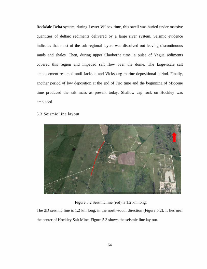
64

Rockdale Delta system, during Lower Wilcox time, this swell was buried under massive

quantities of deltaic sediments delivered by a large river system. Seismic evidence

indicates that most of the sub-regional layers was dissolved out leaving discontinuous

sands and shales. Then, during upper Claoborne time, a pulse of Yegua sediments

covered this region and impeded salt flow over the dome. The large-scale salt

emplacement resumed until Jackson and Vicksburg marine depositional period. Finally,

another period of low deposition at the end of Frio time and the beginning of Miocene

time produced the salt mass as present today. Shallow cap rock on Hockley was

emplaced.

5.3 Seismic line layout

The 2D seismic line is 1.2 km long, in the north-south direction (Figure 5.2). It lies near

the center of Hockley Salt Mine. Figure 5.3 shows the seismic line lay out.

N

Figure 5.2 Seismic line (red) is 1.2 km long.

65

Source: We use the Minivibe to generate a linear sweep from 15 Hz to 160 Hz for 12

seconds and 3 vertical stacks.

Receiver: We use 14-Hz vertical geophones which are planted with 5-m group interval. A

250 Hz high-cut filter on the recorder was applied to eliminate noise.

Recorder: For our multiple channels acquisition purpose, we used Geometrics Geode

system with several 24-channel boxes (A/D converter) that can offer more detailed and

digitized information at one time. After each shot finished, all the data were transmitted

digitally through the data cable and stored in a heavy duty laptop computer as a standard

SEGY file. An operating program called Seismic Controller Software (SCS) installed in

the computer allows us to view shot, line noise and survey parameters simultaneously (Li

Chang, 2013).

Figure 5.3 Seismic line lay out (Courtesy of Li Chang)

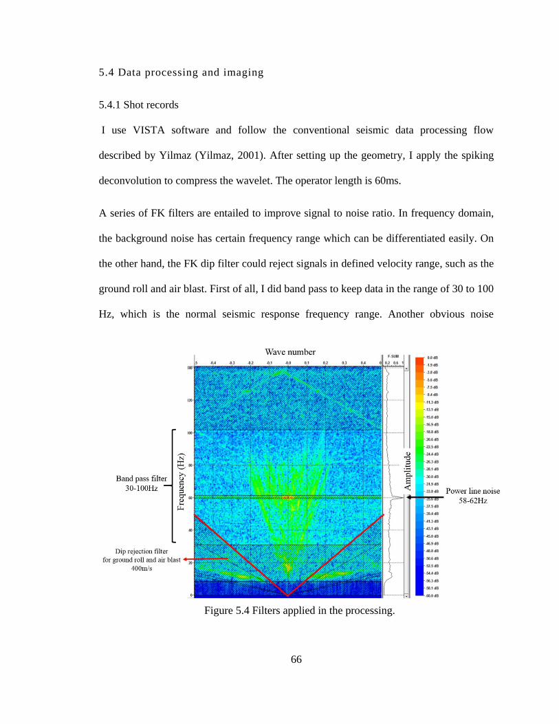
66

5.4 Data processing and imaging

5.4.1 Shot records

I use VISTA software and follow the conventional seismic data processing flow

described by Yilmaz (Yilmaz, 2001). After setting up the geometry, I apply the spiking

deconvolution to compress the wavelet. The operator length is 60ms.

A series of FK filters are entailed to improve signal to noise ratio. In frequency domain,

the background noise has certain frequency range which can be differentiated easily. On

the other hand, the FK dip filter could reject signals in defined velocity range, such as the

ground roll and air blast. First of all, I did band pass to keep data in the range of 30 to 100

Hz, which is the normal seismic response frequency range. Another obvious noise

Figure 5.4 Filters applied in the processing.

67

occurring around 60 Hz is believed to be power line noise. I use 58-62Hz band filter to

reject it. The normal low velocity signals include air blast and ground roll. The air blast

velocity is around 0.34km/s (Dean, 1979), while the velocity of ground roll is about

0.9194 times the shear velocity when Poisson’s ratio is 0.25 (Sheriff and Geldart, 1982).

In this case, I generally have signals under 400m/s rejected by frequency dip rejection

filter. Figure 5.4 shows the main filters applied in the process.

Figure 5.5 is the refraction crossover plot of travel time and distance from source. Figure

5.6 gives a filtered shot view in density mode. Velocity information is more easily

obtained for each shot gather in density display than in wiggle display. From the seismic

shot record profile, NMO velocities could be picked for main events. The direct wave

appears in the top with velocity around 0.79km/s. It is covered soon by the refraction of

sedimentary half-space with the velocity around 1.8km/s. The steep line in the shallow

center is ground roll with low velocity. The hyperbola with extremely high velocity

around 5.5 km/s is the first reflection that we have. Another reflection we have occurs in

the bottom, with velocity around 4.2km/s.

From the seismic refraction crossover of travel time and distance from source, we are

able to calculate the depth of three main refractors that marked in Figure 5.5. The depth

of interface could be calculated by:

𝑧𝑐 =𝑥𝑐2√𝑣𝑝2 − 𝑣𝑝1𝑣𝑝2 + 𝑣𝑝1

68

𝑧𝑐 is the depth of the cth layer, 𝑥𝑐 is the travel distance in the cth layer. 𝑣𝑝1is the velocity

of upper layer and 𝑣𝑝2 is the velocity of lower layer. The first interface that we interpret

as the boundary of unconsolidated weathering layer and sedimentary layer (including

sand, clay, calcite, and gypsum). The distance from source is around 25 m. Our

Distance (m)

0 300 600 900 1200

Tim

e (m

s)

25

0 20

0 1

50

1

00

50

0

Vdirect=790m/s

Vrefraction1=1800m/s

Vrefraction2=5500m/s

Vreflection=4300m/s

𝐷1 = 7.8m

𝐷2 = 42m

Figure 5.6 Shot record (density display).

Figure 5.5 Refraction crossover of travel time versus distance from source.

69

interpreted depth for the weathering layer is 7.8 m (25 ft). And the second layer that we

interpret as sedimentary has the distance to source of 120 m. The depth for sedimentary is

around 42 m (138 ft). So the anhydrite with the velocity of 5.5 km/s occurs around 50 m

(164 ft) in this shot record. One drilled well in Hockley (Figure 5.7) shows the

occurrence of anhydrite shows around 40 m (131 ft). Our interpretation of anhydrite is

Figure 5.7 Section encountered in Hockley shaft. Vertical scale in feet and inches (Teas,

1931).

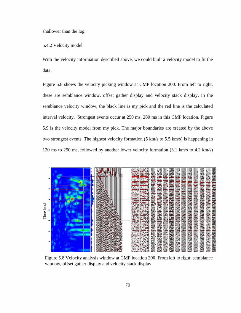
70

shallower than the log.

5.4.2 Velocity model

With the velocity information described above, we could built a velocity model to fit the

data.

Figure 5.8 shows the velocity picking window at CMP location 200. From left to right,

these are semblance window, offset gather display and velocity stack display. In the

semblance velocity window, the black line is my pick and the red line is the calculated

interval velocity. Strongest events occur at 250 ms, 280 ms in this CMP location. Figure

5.9 is the velocity model from my pick. The major boundaries are created by the above

two strongest events. The highest velocity formation (5 km/s to 5.5 km/s) is happening in

120 ms to 250 ms, followed by another lower velocity formation (3.1 km/s to 4.2 km/s)

Figure 5.8 Velocity analysis window at CMP location 200. From left to right: semblance

window, offset gather display and velocity stack display.

Tim

e (m

s)

71

from 260 ms to 400 ms. Velocity in shallow formation ranges from 1.5 km/s to 3 km/s

while in deeper section from 4 km/s to 5 km/s. Figure 5.8 shows the velocity model

generated from semblance velocity picking.

5.5 Interpretation

The report of Hockley Salt Mine gives a structure view of this flat-top salt dome. It is

documented to have cap which is composed of a porous cavernous limestone. Beneath

the limestone sheet occurs a thick bed of dense finely crystalline anhydrite. The anhydrite

lies directly on the salt (Deussen and Lane, 1925). Our seismic line lies in the center of

the salt dome, and we are expected to see reflections mainly from the flat boundaries of

these three formations.

Figure 5.9 Velocity model generated form semblance velocity analysis.

Vel

oci

ty (

m/s

)

Tim

e (m

s)

72

Name of well Cap rock(ft) Limestone

(ft)

Anhydrite(ft) Rock

salt(ft)

John Warren No.1(L&B) 237 237-541

John Warren No. 1(Spear) 100

John Warren No. 1(TTC) 114-1109 231-258 1109-3123

John Warren No. 1(H) 14-730

John Warren No. 2(H) 550-863 750

John Warren No. 3(H) 438-545

John Warren No. 4(H) 400

John Warren No. 5(H) 400

John Warren No.2(G) 813 813-849

John Warren No.3(G)

John Warren No.4(G) 355-369

John Warren No.5 (G) 163 330-571

John Warren No.8(G) 855-920

John Warren No.9 (G) 99 272

John Warren No.10(G) 327 327-464

John Warren No.11(G) 909 909-974

John Warren No.13(G) 3197

John Warren No.16(G) 338

John Warren No.17(G) 219 219

John Warren No.18(G) 131 1059

John Warren No.19(G) 265 1030

John Warren No.1(T) 872-1080 1080-1114 1114-1145

John Warren No.6(T) 187-192

John Warren No.7(T) 252 252-1080 1080-1088

John Warren No.8(T) 165

John Warren No.11(T) 183

John Warren No.12(T) 186

John Warren No.13(T) 1820

John Warren No.14(T) 101 135

John Warren No.19(T) 368

Table 5.1 is a list of wells drilled through Hockley with the cap and salt information in it.

It is modified after Deussen and Lane’s report in 1925. It mainly shows the occurrence of

cap rock, limestone, anhydrite and salt. The cap rock and rock salt are not continuous

Table 5.1. Some wells in Hockley Salt Mine with cap rock and salt depth (Deussen and

Lane, 1925).

73

from the log data. It shows main anhydrite appears mostly around 90 to 245 m (300 to

800 ft). The top of salt from log shows up most likely at 335 m (1100 ft).

From our seismic data, the most prominent feature from the shot gather and velocity

analysis is the occurrence of three strong events around 80 ms, 200 ms and 250 ms,

respectively (Figure 5.10). They create three major boundaries in velocity model.

As the Hockley Salt Mine report (Deussen and Lane, 1925) described, the cap rock

mainly contains limestone and anhydrite. The main anhydrite-salt contact is sharp and

practically horizontal (Teas, 1936). From the velocity range, we interpret the first

boundary as the interface of upper sedimentary as well as gypsum (1.5 km/s to 2.5 km/s)

and limestone (3.5 km/s to 4.0 km/s), and the second boundary as the interface of

limestone and anhydrite (4.5 km/s to 5.5 km/s). The third boundary is the interface of

anhydrite and top of salt (4.0 km/s to 4.5 km/s).

40

0

3

00

2

00

10

0

0

Tim

e (m

s)

S N

0 300 600 900 1200

Distance (m)

Figure 5.10 Seismic brute stack section showing strong reflectors.

74

Another feature shows in our seismic profile is the inconsistence events and the energy

scattering in the north part. It is not likely the artifact caused by the processing methods

since the inconsistence and energy scattering do not change with different filter

parameters or velocity models. If these reflections are real, there might be some

inconsistent structures such as faults.

75

Chapter 6

Conclusions

This thesis studies the salt properties on the earth, especially in the Gulf of Mexico area,

from three aspects: lab measurements, well-log data, and 2D surface seismic data.

Generally, the lab measurements investigate salt anisotropy properties in different salt

samples. The study of log data provides empirical relationship between salt velocity and

depth as well as density in the Gulf of Mexico area. The 2D surface seismic survey in

Hockley Salt Mine provides a typical salt structure in the Gulf of Mexico area.

Prominent anisotropy shows in two types of salt samples from ultrasonic measurements:

our pure halite samples and fractured salt samples taken from stressed salt formation. The

anisotropy parameters are calculated for pure halite which shows cubic symmetry. Minor

anisotropy shows in the salt cores, which have crystals uniformly distributed and no

obvious fractures. The measurements suggest two scenarios where seismic anisotropy of

salt might happen: one is the areas with large pure, undeformed halite crystal formations,

such as North Williston Basin and Michigan Basin. Another is the area with dominant

stresses or preferred orientation fractures. Lineation of salt crystals is better developed in

impure, anhydrite-bearing salt than in masses of very pure halite (Balk, 1953). There is a

third possible situation that I did not explore in the lab: the recrystallization and

realignment of salt crystals in the formation. In other cases, salt behaves isotropically.

76

We also consider how much difference cubic anisotropy could make to reflections and

travel time in the field. Numerical models give an idea by using the cubic anisotropy

parameters calculated from pure halite samples. The travel time ramifications calculated

in a 1km-thick 3D single-layer model gives a maximum difference of 20ms for one way

P-wave travel times. Detailed quantification for P-wave, SH-wave and SV-wave could

provide corrections for velocity models of pure salt formation. If a cubic anisotropic

medium was interpreted as an isotropic one, the P-wave reflection events would appear

shallower.

The log data in the Gulf of Mexico area provide empirical relationships between velocity

and depth as well as density in this area. Least-square line curve fitting gives a

relationship between velocity and depth. However, we do not see a trend for the

relationship between velocity and density.

A 1.2 km surface seismic line over the Hockley Salt Mine, a typical salt dome in the Gulf

of Mexico, gives a view of salt structure. Strong reflections from limestone, anhydrite,

and the top of salt are interpreted in the seismic profile. Combined with the velocity

model, I have inferred aspects of a salt dome structure. The structure bears resemblance

to log data. The main formations in the seismic line over the Hockley Salt Mine appear

flat and coherent. Structures change in the south end of the seismic line, which could be

evidence of faults. Interpreted velocities for the anhydrite and salt are around 5.5 km/s

and 4.5 km/s, respectively. The velocities of salt is similar to what we have from log data

(dominant velocity around 4.46 km/s) and the lab measurement under confining pressure

(around 4.7 km/s). From refraction crossover analysis of one shot record, we find depth

77

for the weathering layer is 7.8 m (25 ft). And the second layer that we interpret as

sedimentary (including sand, clay, calcite and gypsum) is around 42 m (138 ft) thick. The

anhydrite with the velocity of 5.5 km/s occurs around 50 m (164 ft) in depth.

Through this study, we have achieved a better understanding of salt properties and have

provided values for salt velocity modeling for pre-salt and sub-salt imaging in the Gulf of

Mexico area.

78

References

Balk, R., 1953, Salt Structure of Jefferson Island Salt Dome, Iberia and Vermilion

Parishes, Louisiana: AAPG Bulletin, 37, 2455-2474.

Bishop, W. F., 1968, Petrology of upper Smackover limestone in North Haynesville field,

Claiborne Parish, Louisiana: AAPG Bulletin, 52, 92-128.

Brown, R. J., and Z. Sun, 1993, An underground seismie-anisotropy experiment in a salt

mine: CREWES Research Report, Univ. of Calgary.

Chapman, L. C., 1923, The Hockley Salt Dome: AAPG Bulletin, 7, 297-299.

Crain, E.R., 1986, The Log Analysis Handbook Volume 1: Quantative Log Analysis

Methods, Tulsa, OK: Penn Well, 44, 91-95.

Daniels, J. J., R. J. Hite, and J. H. Scott, 1980, Geophysical well-log measurements in

three drill holes at Salt Valley, Utah: Geological Survey, Denver, CO (USA).

Dean, E., 1979, Atmospheric effects on the speed of sound: Atmospheric Science

Laboratory, Tech. Rep. ASL-CR-79-0100-4.

Deussen, A., and L. L. Lane, 1925, Hockley Salt Dome, Harris County, Texas: AAPG

Bulletin, 9, 1031-1034.

Gardner, G., L. Gardner, and A. Gregory, 1974, Formation velocity and density-the

diagnostic basics for stratigraphic traps: Geophysics, 39, 770-780.

Gebrande, H., H. Kern, and F. Rummel, 1982, Landolt-Börnstein numerical data and

functional relationship in science and technology: Group V. Geophysics and

Space Research, Physical Properties of Rocks, Subvolume b, 1, 1-223.

79

Gilreath, J., 1983, Log Responses to Salt: Salt Domes of South Louisiana, New Orleans

Geol. Soc.: 3, 103-121.

Hamlin, H. S., 2006, Salt domes in the Gulf Coast aquifer: Aquifers of the Gulf Coast of

Texas, Mace, RE, Davidson, SC, Angle, ES, and Mullican, WF, eds., Texas

Water Development Board, Report, 365, 217-230.

Hewitt, D. F., 1962, Salt in Ontario: Dept. of Mines, Toronto

Hite, R. J., and S. W. Lohman, 1973, Geologic appraisal of Paradox basin salt deposits

for waste emplacement: U.S. Geological Survey Open-File Report, 4339-6, 75.

Huang, Y., D. Lin, B. Bai, S. Roby, and C. Ricardez, Year, Pre-salt Depth Imaging of the

Deepwater Santos Basin, Brazil: 72nd EAGE Conference & Exhibition.

Hudec, M. R., and M. Jackson, 2009, Interaction between spreading salt canopies and

their peripheral thrust systems: Journal of Structural Geology, 31, 1114-1129.

Landrø, M., C. Puigdefabregas, and B. Arntsen, 2011, Anisotropy in the salt outcrop at

Cardona, Catalonia–implications for seismic imaging: First Break, 29, 41-45.

Lane, D., 2008, The Salt Enthusiast's Scrapbook: Lulu. com.

Lines, L. R., and R. T. Newrick, 2004, Fundamentals of geophysical interpretation:

Society of Exploration Geophysicists.

Lishman, J. R., 1961, Salt bed identification from unfocused resistivity logs: Geophysics,

26, 320-341.

Pauling, L., 1929, The principles determining the structure of complex ionic crystals:

Journal of the American Chemical Society, 51, 1010-1026.

80

Raymer, D., J. Kendall, D. Pedlar, R. Kendall, M. Mueller, and G. Beaudoin, 2000, The

significance of salt anisotropy in seismic imaging: Proceedings of 70th Annual Int.

Meeting of the Soc. Explor. Geophys., Calgary.

Raymer, D. G., and J. Kendall, 1997, Potential pitfalls in imaging salt structures due to

preferred crystal orientation and seismic anisotropy: 1997 SEG Annual Meeting,

Society of Exploration Geophysicists.

Reil, K., and S. Collaboration, 2006, SalSA: a teraton UHE neutrino detector:

PARTICLES AND NUCLEI: Seventeenth Internatinal Conference on Particles

and Nuclei, AIP Publishing, 980-982.

Salvador, A., 1991, Origin and development of the Gulf of Mexico basin: The Gulf of

Mexico basin, The Geology of North America, J, 389-444.

Sheriff, R. E., and L. P. Geldart, 1982, Exploration seismology: Cambridge Univ. Press.

Sondergeld, C., and C. Rai, 1992, Laboratory observations of shear-wave propagation in

anisotropic media: The leading edge, 11, 38-43.

Steele, K., and S. J. Haynes, 2000, Mines and wines: Industrial minerals, geology and

wineries of the Niagara region, field trip guidebook.

Sun, Z., 1994, Seismic anisotrophy in salt from theoretical study, modelling and field

experiments: M.Sc. thesis, University of Calgary.

Teas, L., 1936, Hockley Salt Shaft, Harris County, Texas: AAPG Special Volumes, 136-

140.

Teas, L. P., 1931, Hockley Salt Shaft, Harris County, Texas: AAPG Bulletin, 15, 465-469.

Thomsen, L., 1986, Weak elastic anisotropy: Geophysics, 51, 1954-1966.

81

Tingay, M. R., R. R. Hillis, C. K. Morley, R. C. King, R. E. Swarbrick, and A. R. Damit,

2009, Present-day stress and neotectonics of Brunei: Implications for petroleum

exploration and production: AAPG Bulletin, 93, 75-100.

Tixier, M., and R. Alger, 1970, Log evaluation of nonmetallic mineral deposits:

Geophysics, 35, 124-142.

Volarovich, M. P., R. S. Akulova, and E. I. Baiuk, 1986, Elasticity of halogen rocks at

high pressures: Moscow Izdatel Nauka, 1.

West, A. R., 1984, Solid state chemistry and its applications: John Wiley & Sons, 596.

Yilmaz, Ö., 2001, Seismic data analysis: Society of Exploration Geophysicists Tulsa.

82

Appendix

Velocities in cubic-symmetry medium

The phase velocity is derived from the first Green-Christoffel equations.

0)(2

kikphik UV (A-1)

The second-rank tensor:

ljijklik nnC (A-2)

is called Green-Christoffel tensor. kU is the displacement in direction k . It depends both

on elastic tensor of the medium studied and on the direction n of the wave normal. The

eigenvalue of ik is

2

phV and the eigenvector of it is kU . This equation (A-1) has non-

trivial solution when:

02

ikphik V (A-3)

To solve the phase velocity, we need solve the cubic equation:

0rrr- 32

2

1

3 III (A-4)

where,

2

phVr (A-5)

1I , 2I and 3I are the invariants of tensor

ik . Taking (A-2) into account, we could have:

83

325631152116

2

355

2

266

2

11111 222 nnCnnCnnCnCnCnC

322431462126

2

344

2

222

2

16622 222 nnCnnCnnCnCnCnC

323431452126

2

333

2

244

2

15533 222 nnCnnCnnCnCnCnC

323431142112

2

346

2

226

2

11612 222 nnCnnCnnCnCnCnC

323631132114

2

335

2

246

2

11513 222 nnCnnCnnCnCnCnC

322331362146

2

334

2

224

2

15623 222 nnCnnCnnCnCnCnC (A-6)

Here I rewrite the expressions in terms of angles ϴ and φ as shown in the following plot:

cossin1 n

sinsin2 n

cos3 n (A-7)

The algebraic expression of phase velocities in terms of arbitrary angle ϴ and ϕ is very

complicated without simplified notations. In the thesis we only use the algebraic

expressions for velocity in symmetric axes directions and on symmetric plane.

φ

ϴ

n1

n2

n3

84

For cubic-symmetric media, we have the solutions in the three symmetric-axes directions

as:

11CV P

ph

(A-8)

44CVV SH

ph

SV

ph

(A-9)

While in the symmetric planes, for example when 0 , the velocities could be

expressed in terms of ϕ as:

2

2 4411 KCCV P

ph

(A-10)

2

2 4411 KCCV SV

ph

(A-11)

44CV SH

ph

(A-12)

2

444411

2

11

2

4412

22

12

2

4411

22

11

4

4412

42

12

4

4411

42

11

2sin8sin4sin8

sin4sin8sin4sin8sin4

CCCCCCCCC

CCCCCCCK

(A-13)

The velocity distribution is identical on the other two symmetric planes when 2

or

2

.

85

In this thesis, we measured the velocity in the middle of two symmetric axes. Take the

symmetric plane XOZ for example, we are talking about the direction that 0 and

4

.

The solution in this direction is:

2

22 134411 CCCV P

ph

(A-14)

2

2 1311 CCV SV

ph

(A-15)

44CV SH

ph

(A-16)

The group velocity is derived from the second Green-Christoffel equation.

kiijkljl UUC (A-17)

ljl

ph

g

j nVk

V

1 (A-18)

where ω is angular frequency (usually expressed in radians per second), and k is the

angular wavenumber (usually expressed in radians per meter).

In this thesis, the expressions of group velocity as well as the phase velocity are not given

at an arbitrary angle in terms of angles ϴ and φ. But the numerical values for all

directions are calculated based on the general expressions (A-5) and (A-18).