Embed Size (px)
Citation preview
Elastic and Viscous Properties of Polyolefin Melts with Different Molecular Structures Investigated in Shear and Elongation
Elastische und viskose Eigenschaften von Polyolefinschmelzen mit verschiedenem molekularen Aufbau untersucht in Scherung und
Dehnung
Der Technischen Fakultät der
Universität Erlangen-Nürnberg
zur Erlangung des Grades
DOKTOR-INGENIEUR
vorgelegt von
Julia Antonia Resch
Erlangen - 2010
Als Dissertation genehmigt von
der Technischen Fakultät der
Universität Erlangen-Nürnberg
Tag der Einreichung: 07.01.2010
Tag der Promotion: 25.02.2010
Dekan: Prof. Dr.-Ing. Reinhard German
Berichterstatter: Prof. Dr. Helmut Münstedt
A.Univ.-Prof. Dr. Alois Schausberger

Table of Contents
I
Table of Contents
1. INTRODUCTION 1
2. GERMAN INTRODUCTION 4
3. LITERATURE 8
3.1. Viscous Properties in Shear 8 3.1.1. Influence of Molar Mass 8 3.1.2. Influence of Molar Mass Distribution 9 3.1.3. Influence of Long-Chain Branching 9
3.2. Elastic Properties in Shear 11 3.2.1. Measuring the Recoverable Compliance 11 3.2.2. Influence of Molar Mass and Molar Mass Distribution 12 3.2.3. Influence of LCB and SCB 14 3.2.4. Elastic Properties in the Nonlinear Regime 17
3.3. Viscous Properties in Uniaxial Elongation 19
3.4. Elastic Properties in Uniaxial Elongation 21
3.5. Extrudate Swell 22
3.6. Temperature Dependence of Rheological Properties 24
3.7. Summary of Literature Survey and Aim of the Work 26
4. METHODS FOR MOLECULAR CHARACTERIZATION 28
4.1. Size Exclusion Chromatography (SEC) with Coupled Multi-Angle Laser Light Scattering (MALLS) 28
4.2. Differential Scanning Calorimetry (DSC) 29
4.3. Fourier Transformation Infrared Spectroscopy (FT-IR-Spectroscopy) 30 4.3.1. Determination of Comonomer Type for mLLDPE 30 4.3.2. Determination of Isotacticity and Comonomer for PP 30
5. RHEOLOGICAL METHODS 32
5.1. Rheological Methods in Shear 32 5.1.1. Sample Preparation 33 5.1.2. Dynamic-Mechanical Experiments 33 5.1.3. Creep-Recovery Experiments 34
5.2. Determination of the Extrudate Swell 37
5.3. Rheological Methods in Elongation 38 5.3.1. Setup of the Elongational Rheometer 38 5.3.2. Sample Preparation 39 5.3.3. Stressing Experiments 40 5.3.4. Creep-Recovery Experiments 41

II Table of Contents
6. CHARACTERIZATION OF MATERIALS 45
6.1. Polyethylenes 45 6.1.1. Mean Square Value of the Radius of Gyration as a Function of Mw 49 6.1.2. Correlation between Zero Shear-Rate Viscosity and Mw 52 6.1.3. Investigations on Crystalline Structure by DSC 53
6.2. Polypropylenes 54
7. RHEOLOGICAL MEASUREMENTS IN SHEAR 59
7.1. Dynamic-Mechanical Experiments 59
7.2. Creep-Recovery Experiments 63 7.2.1. Linear Viscous Properties 63 7.2.2. Linear Elastic Properties 69 7.2.3. Temperature dependence of Jr(tr) and Je
0 for PE and PP 79 7.2.4. Nonlinear Creep-Recovery Experiments 94 7.2.5. Correlation of Stress Dependence of Viscosity and Elasticity with Molecular Structure 104 7.2.6. Discussion: Stress Dependence of Je and η 110
8. RHEOLOGICAL MEASUREMENTS IN ELONGATION 114
8.1. Stressing Experiments 114
8.2. Creep-Recovery Experiments 116 8.2.1. Viscous Properties 116 8.2.2. Elastic Properties 121 8.2.3. Comparison between Viscous and Elastic Properties 125
9. COMPARISON OF RHEOLOGICAL PROPERTIES IN SHEAR AND ELONGATION 127
9.1. Stress-Dependent Viscosities and Steady-State Elastic Compliances in Shear and Elongation 127
9.2. Discussion: Stress-Dependent Viscosities and Steady-State Elastic Compliances in Shear and Elongation 131
10. SUMMARY AND OUTLOOK 134
11. GERMAN ABSTRACT 139
12. APPENDIX 143
12.1. Measuring the Recoverable Compliance with the AR-G2 143
12.2. SEC-MALLS 149
12.3. δ(|G*|)-Plots of mLLDPE 3 and mLLDPE 4 151
12.4. Mastercurves of J(t) and Jr(tr) in the Linear and Nonlinear Regime 153
12.5. Determination of Relaxation and Retardation Spectra 156

Table of Contents
III
12.6. Sample Preparation for Elongational Rheology 160
12.7. Zero Shear-Rate Viscosities at Different Temperatures 161
12.8. Temperature Rising Elution Fractionation (TREF) 162
12.9. Stress Dependence of Viscosity and Elasticity at Different Temperatures 163
12.10. Numerical description of the stress dependence of Je 166
12.11. Determination of Extrudate Swell 168
12.12. Stressing Experiments in Elongation 173
12.13. Homogeneity of Deformation in Tensile Creep-Recovery Tests 177
12.14. Abbreviations and Symbols 179
13. REFERENCES 184
14. ACKNOWLEDGEMENT 194


Inhaltsverzeichnis
V
Inhaltsverzeichnis 1. EINLEITUNG 1 2. DEUTSCHE EINLEITUNG 4 3. LITERATUR 8 3.1. Viskose Eigenschaften in Scherung 8 3.1.1 Einfluss der Molmasse 8 3.1.2 Einfluss der Molmassenverteilung 9 3.1.3 Einfluss von Langkettenverzweigungen 9
3.2. Elastische Eigenschaften in Scherung 11 3.2.1 Bestimmung der reversiblen Nachgiebigkeit 11 3.2.2 Einfluss der Molmasse und der Molmassenverteilung 12 3.2.3 Einfluss von Lang- und Kurzkettenverzweigungen 14 3.2.4 Elastische Eigenschaften in Scherung im nichtlinearen Bereich 17
3.3. Viskose Eigenschaften in uniaxialer Dehnung 19 3.4. Elastische Eigenschaften in uniaxialer Dehnung 21 3.5. Strangaufweitung 22 3.6. Temperaturabhängigkeit von rheologischen Eigenschaften 24 3.7. Zusammenfassung der Literaturstudie und Ziel der Arbeit 26 4. METHODEN DER MOLEKULAREN CHARAKTERISIERUNG 28 4.1. Gelpermeationschromatographie (SEC) gekoppelt mit Vielwinkellichtstreuung (MALLS) 28 4.2. Dynamische Differenzkalorimetrie (DSC) 29 4.3. Fourier-Transformation Infrarotspektroskopie (FT-IR-Spektroskopie) 30 4.3.1 Bestimmung der Comonomerart von mLLDPE 30 4.3.2 Bestimmung der Isotaktizität und des Comonomeranteils von PP 30 5. RHEOLOGISCHE METHODEN 32 5.1. Rheologische Methoden in Scherung 32 5.1.1 Probenvorbereitung 33 5.1.2 Dynamisch-mechanisches Experiment 33 5.1.3 Kriecherholversuch 34 5.2. Bestimmung der Strangaufweitung 37 5.3. Rheologische Methoden in Dehnung 38 5.3.1 Aufbau des Dehnrheometers 38 5.3.2 Probenvorbereitung 39 5.3.3 Spannversuch 40 5.3.4 Kriecherholversuch 41
VI Inhaltsverzeichnis
6. CHARAKTERISIERUNG DER MATERIALIEN 45 6.1. Polyethylene 45 6.1.1 Erwartungswert des Quadrates des Gyrationsradius als Funktion von Mw 49 6.1.2 Beziehung zwischen Nullviskosität und Mw 52 6.1.3 Analyse der Kristallinität mittels DSC 53 6.2. Polypropylene 54 7. RHEOLOGISCHE MESSUNGEN IN SCHERUNG 59 7.1. Dynamisch-mechanische Experimente 59 7.2. Kriecherholversuche 63 7.2.1 Lineare viskose Eigenschaften 63 7.2.2 Lineare elastische Eigenschaften 69 7.2.3 Temperaturabhängigkeit von Jr(tr) und Je
0 für PE und PP 79 7.2.4 Nichtlineare Kriecherholversuche 94 7.2.5 Korrelation der Spannungsabhängigkeit von Viskosität und Elastizität
mit dem molekularen Aufbau 104 7.2.6 Diskussion: Spannungsabhängigkeit von Je und η 110 8. RHEOLOGISCHE MESSUNGEN IN DEHNUNG 114 8.1. Spannversuche 114 8.2. Kriecherholversuche 116 8.2.1 Viskose Eigenschaften 116 8.2.2 Elastische Eigenschaften 121 8.2.3 Vergleich zwischen viskosen und elastischen Eigenschaften 125 9. VERGLEICH DER RHEOLOGISCHEN EIGENSCHAFTEN IN SCHERUNG UND DEHNUNG 127 9.1. Spannungsabhängige Viskositäten und elastische Gleichgewichtsnachgiebigkeiten in Scherung
und Dehnung 127 9.2. Diskussion: Spannungsabhängige Viskositäten und elastische Gleichgewichtsnachgiebigkeiten
in Scherung und Denhung 131 10. ZUSAMMENFASSUNG UND AUSBLICK 134 11. DEUTSCHE ZUSAMMENFASSUNG 139 12. ANHANG 143 12.1. Bestimmung der reversiblen Nachgiebigkeit mit dem AR-G2 143 12.2. SEC-MALLS 149 12.3. δ(|G*|)-Auftragung von mLLDPE 3 und mLLDPE 4 151 12.4. Masterkurven von J(t) und Jr(tr) im linearen und nichtlinearen Spannungsbereich 153 12.5. Bestimmung von Relaxations- und Retardationszeitspektren 156
Inhaltsverzeichnis
VII
12.6. Vorbereitung der Dehnproben 160 12.7. Nullviskositäten bei verschiedenen Temperaturen 161 12.8. Elutionsfraktionierung bei steigender Temperatur (TREF) 162 12.9. Spannungsabhängigkeit von Viskosität und Elastizität bei verschiedenen Temperaturen 163 12.10. Numerische Beschreibung der Spannungsabhängigkeit von Je 166 12.11. Bestimmung der Strangaufweitung 168 12.12. Spannversuche in Dehnung 173 12.13. Homogenität der Deformation im Kriecherholversuch in Dehnung 177 12.14. Verwendete Abkürzungen und Symbole 179 13. LITERATURVERZEICHNIS 184 14. DANKSAGUNG 194


Introduction
1
1. Introduction In this thesis, the influence of the molecular structure on the elastic and viscous properties of
polymer melts is investigated. Polyolefins (polyethylene and polypropylene) are judged to be
the best materials to tackle this task as many grades of various manufacturers are
commercially available.
Polyolefins are semi-crystalline polymers whose temperature dependence of the rheological
properties of the melt is not as pronounced as for amorphous materials such as PS or PMMA.
Another positive issue for the rheological investigations of polyolefin melts is the moderate
melting temperature of PE varying between 80 and 130°C depending on the polyethylene
type and PP being around 165°C for homopolymers. Technical polymers, such as PEEK or
PA, have much higher melting temperatures, and thus, often limited thermal stabilities
restricting the possible rheological measurements. However, despite the progresses in
catalysts research the structure of polyolefins cannot be as precisely adjusted as it is possible
for anionic PS, for example.
PE and PP are besides PVC, PS, and PET quantitatively the most important plastics
worldwide. Packaging is the biggest end-use application of PE. Polypropylene has compared
to polyethylene a higher melting temperature and is, therefore, used for purposes, especially
in the automobile industry, where due to the stronger requirements concerning temperature
polyethylene is not applicable. Favourable for some applications is also its lower density
compared to PE. Foams of polypropylene are used in construction, packaging, automotive
industry as well as homewares and furniture.
For PE a broad scope of molecular architectures is possible that also determine the processing
behaviour and the mechanical properties of the polymer. Different types of PE are classified
according to their density. As main groups LDPE (low-density polyethylene), LLDPE (linear-
low-density polyethylene), and HDPE (high-density polyethylene) are distinguished.
LPDE is synthesized at high pressures (1000 – 3000 bar) and at high temperatures (approx.
80 - 300°C) in a radical reaction (Domininghaus et al., 2008). Because of the production
process it has a long-chain branched structure with excellent processing behaviour, e.g., shear
thinning and strain hardening. Disadvantages of LDPE are the inferior mechanical properties
compared to LLDPE whose processing behaviour is less favourable than for LDPE. Therefore,
for industrial applications sometimes blends of these two materials are used.
LLDPE and HDPE are synthesized using catalysts at temperatures below 100°C and
pressures below 50 bar (Keim, 2006). Ziegler-Natta-catalysts (Z/N-catalysts) were the first

2 Introduction
catalysts for the production of linear polyethylenes. Unless no comonomer is added these PE
have no short-chain branches, and thus, a high crystallinity. By the addition of comonomers
(alpha-olefins) not only the crystallinity decreases but also the mechanical properties can be
adjusted using different types and contents of comonomers. Main disadvantages of the Z/N-
catalysts are their incapability to polymerize olefins longer than octene, residual traces of the
catalyst in the polymer restricting the application, e.g., in medical applications, and the
inhomogeneous insertion of the comonomer, which may cause phase separations (e.g. Stadler
et al., 2005). Another class of catalysts are the metallocene catalysts that overcome some
problems of the Z/N-catalysts. Because of the controlled reaction mechanism polyethylenes
possessing a narrow molar mass distribution (Mw/Mn ≈ 2) and a more homogeneous
comonomer insertion can be produced. In addition, mLLDPE containing small contents of
long-chain branches can be synthesized, whose molar mass distribution and mechanical
properties are similar to those of linear mLLDPE but whose processing behaviour is
improved.
Commercially available linear polypropylene is mainly produced using Ziegler-Natta-
catalysts. The commercial synthesis takes place at temperatures of 60 – 90°C and pressures
above 30 bar (Lieberman and LeNoir, 1996). The isotactic structure generated by the catalysts
is responsible for the semi-crystallinity of the material. The order of the methyl side groups
(isotactic, syndiotactic, atactic) determines the mechanical properties of the material. As in
the case of polyethylene, metallocene catalysts allow the synthesis of polypropylene with a
narrower polydispersity and, additionally, a defined variation of tacticity (Sinn and
Kaminsky, 1980). Isotactic and syndiotactic PP with narrow polydispersities of 2 - 3 are
commercially available since the mid 1990s.
Long-chain branches in PP can be generated directly in the polymerisation process by using
longer comonomers (Walter et al., 2001), special catalyst systems (Weng et al., 2002) or
through modification of linear PP with electron-beam irradiation or using chemical methods
(Scheve et al., 1986, Yoshii et al., 1996). The post-reactor insertion of long-chain branches is
common for commercially available LCB-PP. Peroxides and electron beam irradiation cause
chain scission to generate free radicals, which can recombine to form branched chains.
Polymer melts exhibit a complex rheological behaviour depending on the type of deformation
– shear, elongation or a combination of both – and the strength of deformation. The response
of the material to the stress is generally a combination of viscous and elastic behaviour.
Depending on the processing conditions, the viscosity during the extrusion process may vary
within orders of magnitude. For other processing techniques, such as blow-moulding, deep-

Introduction
3
drawing or film-blowing, the elongational properties of the polymer melt are of essential
relevance. In extrusion processes, the elastic properties are responsible for the extrudate swell
that reflects the orientation of the molecules generated during processing and also influences
the properties of the finished product.
An important task for the understanding of the behaviour of polymer melts during processing
is an extensive rheological characterization. The rheological behaviour is determined by the
molecular structure of the material, which is generated during synthesis. Therefore, rheology
is a versatile tool to establish a connection between the molecular architecture and the
processing properties.
The viscous properties of polymer melts have been systematically and extensively
investigated. For the elastic properties, however, precise studies concerning the influence of
molecular structure, such as molar mass, molar mass distribution, and long-chain branching,
are missing. The stress dependence of rheological quantities is an important issue, too. For the
viscosity of polyolefin melts, this effect has been widely investigated. It is commonly known
that polymer melts exhibit shear thinning whose characteristics depend on the molecular
structure of the material. However, little is known about the stress dependence of elastic
properties and their correlation with the molecular architecture. Both, viscosity and elasticity
of the polymer melt influence the behaviour during processing, which typically takes place at
high stresses or shear rates.
In this work, both shear and elongational rheology are employed. Shear rheology is a widely
used analysis method. Elongational experiments, however, are not so common because of the
missing suitable measuring equipment and expertise.
This thesis primarily deals with the investigation of elastic properties of polyolefin melts
investigated in shear and elongation in the linear and nonlinear stress regime. The main aim
of this work is to find relationships between molecular parameters, such as molar mass, molar
mass distribution, and branching structure, and the elastic properties of polyolefin melts using
shear and elongational rheology. As also the viscous properties can be determined from the
measurements performed a comparison between the stress dependence of viscosity and
elasticity is possible, too.
4 German Introduction
2. German Introduction
Das Ziel dieser Arbeit ist die Untersuchung des Einflusses des molekularen Aufbaus auf
elastische und viskose Eigenschaften von Polymerschmelzen. Polyolefine (Polyethylen und
Polypropylen) werden als geeignete Materialien erachtet, um dieser Fragestellung
nachzugehen, da kommerziell eine Reihe unterschiedlicher Produkte verschiedener Hersteller
erhältlich ist.
Polyolefine sind teilkristalline Polymere, deren rheologische Eignschaften der Schmelze eine
geringere Empfindlichkeit gegenüber Temperaturänderungen im Vergleich zu amorphen
Materialien, wie PS oder PMMA, besitzen. Einen weiteren Vorteil für die rheologischen
Untersuchungen bieten Polyolfinschmelzen wegen ihres moderaten Schmelzpunkts, der
abhängig vom Polyethylentyp zwischen 80°C und 130°C und für Polypropylen bei ca. 165°C
liegt. Die Schmelzpunkte von anderen technischen Kunststoffen, wie z. B. PEEK oder PA,
sind viel höher, was zu begrenzten thermischen Stabilitäten führt und dadurch die möglichen
rheologischen Messungen einschränkt. Es ist jedoch anzumerken, dass trotz des großen
Fortschritts in der Katalysatorforschung Polyolefine nicht mit einer so definierten Struktur
hergestellt werden können, wie das etwa für anionische PS möglich ist.
PE und PP sind neben PVC, PS und PET die mengenmäßig bedeutendsten Kunststoffe
weltweit. PE kommen am häufigsten in der Verpackungsindustrie zum Einsatz. PP hingegen
eignen sich aufgrund ihres höheren Schmelzpunkts beispielsweise für Anwendungen in der
Automobilindustrie, wo aufgrund der höheren Gebrauchstemperaturen Polyethylene nicht
einsetzbar sind. Für manche Anwendungen vorteilhaft ist auch die niedrigere Dichte von PP
im Vergleich zu PE. Polypropylenschäume finden Einsatz im Baugewerbe, im
Verpackungssektor, im Haushaltswarenbereich und in der Automobil- bzw. Möbelindustrie.
Es gibt eine Vielzahl von Polyethylenen mit unterschiedlichem molekularen Aufbau, der
sowohl das Verarbeitungsverhalten als auch die mechanischen Eigenschaften des Materials
bestimmt. Polyethylene werden nach ihrer Dichte in LDPE (low-density polyethylene,
Polyethylen niederer Dichte), LLDPE (linear-low-density polyethylene, lineares Polyethylen
niederer Dichte) und HDPE (high-density polyethylene, Polyethylen hoher Dichte)
unterschieden. Die Synthese von LDPE erfolgt mittels radikalischer Reaktion bei hohen
Drücken (1000 – 3000 bar) und hohen Temperaturen (ca. 80 – 300°C) (Domininghaus et al.,
2008). Aufgrund ihres Herstellungsverfahrens besitzen PE eine langkettenverzweigte Struktur
mit ausgezeichnetem Verarbeitungsverhalten, wobei hier die hohe Strukturviskosität und die
Dehnverfestigung zu nennen sind. LDPE hat aber schlechtere mechanische Eigenschaften im
German Introduction
5
Vergleich zu LLDPE, welches wiederum ein weniger gutes Verarbeitungsverhalten zeigt.
Darum werden für Industrieanwendungen häufig Blends dieser beiden Materialien eingesetzt.
LLDPE und HDPE werden katalytisch bei Temperaturen unter 100°C und Drücken kleiner
als 50 bar synthetisiert (Keim, 2006). Ziegler-Natta-Katalysatoren (Z/N-Katalysatoren)
kamen als erste Katalysatoren zur Herstellung von Z/N-Polyethylenen zum Einsatz. Ohne
Beigabe von Comonomer besitzen diese Polyethylene keine Kurzkettenverzweigungen und
daher eine hohe Kristallinität. Durch Zugabe von Comonomeren (Alpha-Olefine) sinkt nicht
nur die Kristallinität, sondern auch die mechanischen Eigenschaften können durch Änderung
von Comonomerart und -gehalt variiert werden. Mittels Z/N-Katalysatoren können einerseits
keine längeren Olefine als Okten eingebaut werden, andererseits erfolgt der Einbau des
Comonomers inhomogen, was zur Phasentrennung führt (z. B. Stadler et al., 2005). Einen
Nachteil stellen auch verbleibende Spuren des Katalysators im Polymer dar, die
beispielsweise den Einsatz in der Medizintechnik einschränken. Die Klasse der Metallocen-
Katalysatoren überwindet einige der Schwächen der Ziegler-Natta-Katalysatoren. Aufgrund
des kontrollierten Reaktionsmechanismus können Polyethylene mit einer engen
Molmassenverteilung (Mw/Mn ≈ 2) und einem homogeneren Comonomereinbau hergestellt
werden. Darüber hinaus können mLLDPE mit geringen Gehalten an
Langkettenverzweigungen synthetisiert werden, deren Molmassenverteilung und
mechanische Eigenschaften ähnlich denen der linearen mLLDPE sind, die jedoch ein
verbessertes Verarbeitungsverhalten aufweisen.
Die Herstellung von kommerziell erhältlichen linearen Polypropylenen erfolgt zum
überwiegenden Teil mit Z/N-Katalysatoren bei Temperaturen zwischen 60°C und 90°C und
Drücken größer als 30 bar (Lieberman und LeNoir, 1996). Der Katalysator sorgt für die
isotaktische Struktur des PP, welche für die Teilkristallinität des Materials verantwortlich ist.
Die Anordnung der Seitengruppen (isotaktisch, syndiotaktisch, ataktisch) bestimmt die
mechanischen Eigenschaften des Polymers. Wie für Polyethylen erlauben Metallocen-
Katalysatoren auch die Herstellung von Polypropylenen mit einer engen
Molmassenverteilung. Darüber hinaus ermöglichen sie eine Variation der Taktizität (Sinn und
Kaminsky, 1980). Seit Mitte der 1990er Jahre sind isotaktische und syndiotaktische PP mit
einer Molmassenverteilung zwischen 2 und 3 auch kommerziell erhältlich.
Langkettenverzweigungen können auf verschiedene Weise in Polypropylen eingebracht
werden. Zu nennen sind die direkte Polymerisation mit längeren Comonomeren (Walter et al.,
2001), die Anwendung von speziellen Katalysatorsystemen (Weng et al., 2002) und die
Modifikation von linearen PP mittels Elektronenstrahlmodifizierung oder chemischer

6 German Introduction
Methoden (Scheve et al., 1986, Yoshii et al., 1996); wobei das Einbringen von
Langkettenverzweigungen mittels der letztgenannten Methoden (Post-Reaktor Modifikation)
für kommerzielle LCB-PP üblich ist. Peroxide oder die Bestrahlung mit Elektronen bewirken
Kettenbrüche unter der Erzeugung von freien Radikalen, welche rekombinieren und dadurch
verzweigte Ketten bilden können.
Abhängig von Stärke und Art der Deformation (Scherung, Dehnung oder eine Kombination
von beiden) zeigen Polymerschmelzen ein komplexes rheologisches Verhalten. Die Antwort
des Materials auf die Deformation ist üblicherweise eine Kombination von viskosem und
elastischem Verhalten.
Die Viskosität während des Extrusionsprozesses kann beispielsweise abhängig von den
Verarbeitungsbedingungen um Größenordnungen variieren. Bei anderen
Verarbeitungstechniken, wie dem Blasformen, Tiefziehen oder Folienblasen, spielen die
Dehneigenschaften eine wichtige Rolle. In Extrusionsprozessen sind die elastischen
Eigenschaften für die Strangaufweitung verantwortlich, die die eingebrachten Orientierungen
der Moleküle während der Extrusion widerspiegelt und auch Einfluss auf die Eigenschaften
des fertigen Produkts nimmt.
Das Verständnis des Verhaltens von Polymerschmelzen während der Verarbeitung setzt eine
genaue rheologische Charakterisierung voraus. Da das rheologische Verhalten von der
molekularen Struktur, die während des Herstellungsprozess erzeugt wird, abhängt, ermöglicht
die Rheologie eine Verknüpfung zwischen dem molekularen Aufbau und dem
Verarbeitungsverhalten.
Die viskosen Eigenschaften von Polymerschmelzen wurden systematisch und ausführlich
untersucht. Betreffend die elastischen Eigenschaften fehlen hingegen genaue Studien über
den Einfluss von molekularen Parametern, wie Molmasse, Molmassenverteilung und
Langkettenverzweigungen. Die Spannungsabhängigkeit von rheologischen Eigenschaften ist
ebenfalls ein wichtiger Gesichtspunkt. Allgemein bekannt ist etwa die Strukturviskosität,
welche vom molekularen Aufbau des Materials abhängt. Jedoch wenig bekannt ist über die
Spannungsabhängigkeit der elastischen Eigenschaften und ihrer Verbindung mit der
molekularen Architektur. Sowohl Viskosität als auch Elastizität bestimmen das Verhalten
während Verarbeitungsprozessen, die üblicherweise bei hohen Spannungen oder Scherraten
stattfinden.
Diese Arbeit widmet sich der Scher- und Dehnrheologie gleichermaßen. Scherrheologie ist
eine übliche Analysemethode, Dehnrheologie hingegen ist aufgrund der fehlenden geeigneten
Messsysteme und des notwendigen Know-hows weniger verbreitet.

German Introduction
7
Diese Doktorarbeit hat in erster Linie die Untersuchung der elastischen Eigenschaften von
Polyolefinschmelzen in Scherung und Dehnung im linearen und nichtlinearen
Spannungsbereich zum Thema. Das wichtigste Ziel dieser Arbeit ist Verbindungen zwischen
molekularen Parametern, wie Molmasse, Molmassenverteilung und Verzweigungsstruktur,
und den elastischen Eigenschaften von Polyolefinschmelzen unter Zuhilfenahme von Scher-
und Dehnrheologie zu finden. Da bei den durchgeführten Messungen auch die viskosen
Eigenschaften mitbestimmt werden, erlaubt dies den Vergleich zwischen der
Spannungsabhängigkeit von Viskosität und Elastizität.
8 Literature
3. Literature
3.1. Viscous Properties in Shear
3.1.1. Influence of Molar Mass The zero shear-rate viscosity η0 is determined in the Newtonian viscosity regime and can be
measured in experiments performed in the linear regime of stresses or deformation rates. This
quantity is significantly dependent on the weight average molar mass (Ferry, 1980). Its
dependence is described by:
wMK ⋅= 10η for cw MM < (3.1)
αη wMK ⋅= 20 for cw MM > (3.2)
ec MmM ⋅≈ (3.3)
K1 and K2 are constants depending on the polymer and the temperature. Mc is a critical molar
mass, which is approximately two or three times the entanglement molar mass Me (Ferry,
1980, Fetters et al., 1999). According to the literature, Me lies at around 1900 g mol-1 for
polyethylene and in the range of 5100 and 6900 g mol-1 for isotactic polypropylene
(Graessley and Edwards, 1981, Eckstein et al., 1998, Fetters et al., 1999).
For molar masses smaller than Mc, a proportional relationship between Mw and η0 was found,
whereas for Mw higher than Mc an empirical exponent α in a range between 3.4 and 3.6 is
reported (Laun, 1987, Raju et al., 1979, Jordens et al., 2000, Stadler et al., 2006, Auhl et al.,
2004, Auhl, 2006).
For PP the zero shear-rate viscosity is also dependent on the tacticity of the material. Me is
lower for syndiotactic PP (sPP) and lies according to Eckstein et al. (1998) at around
1700 g mol-1. In addition, the factor K2 of Equation (3.2) depends on the chemical structure of
the polymer. Therefore, an explanation for the around by a factor of 10 higher zero shear-rate
viscosities of sPP compared to isotactic PP (iPP) or atactic PP (aPP) is possible (Eckstein et
al., 1997, Rojo et al., 2004).
In the nonlinear regime, the viscosity becomes dependent on the stress or the strain rate and
decreases with increasing stresses or strain rates. Contrarily to the strong dependence of η0 on
Mw, the shape of the viscosity function is independent of Mw. The stress at the onset of the
shear-thinning regime is independent of molar mass. However, this onset takes place at lower
shear rates that correspond to lower stresses for materials with a higher Mw/Mn (e.g. Schwarzl,
1990, Wood-Adams and Dealy, 2000).

Literature
9
Viscosity functions are of great importance to get an insight into the processing behaviour of
polymer melts. They can be determined by stressing experiments, creep experiments, or
dynamic-mechanical experiments. In the range of higher shear rates, capillary rheology is
used. Models were developed for the description of viscosity functions that make an analysis
of the dependence of the description parameters on molecular quantities possible. The
Carreau-Yasuda model (Carreau, 1968, Yasuda, 1979) shows good results for the description
of various types of viscosity functions. For the viscosity η as a function of shear rate γ& the
equation reads:
an
a1
0 ])(1[)(−
⋅+= γληγη && (3.4)
In the Carreau-Yasuda model λ, a, and n are the description parameters typical of a polymer.
The parameter n originates from the Ostwald-de Waele-law, which gives a relationship
between the shear stress τ and the shear rate γ& .
nγτ &∝ (3.5)
n can be determined if a constant slope of τ as a function of shear rate in a double-logarithmic
plot is attained.
3.1.2. Influence of Molar Mass Distribution The molar mass distribution (MMD) has an influence on the viscosity function, the zero
shear-rate viscosity, however, remains unaffected. For polyethylene the independence of η0
from MMD is shown by Gabriel and Münstedt (2002) for PE having polydispersities between
2 and 4. Gahleitner (2001) and Fujiyama and Inata (2002) prove this for polypropylene with
polydispersities between 2.2 and 9.5.
A broader molar mass distribution leads to a stronger shear-thinning effect and a broader
intermediate regime between the Newtonian and the shear-thinning regime (Laun, 1987).
3.1.3. Influence of Long-Chain Branching For long-chain branched polymers, the relation between η0 and Mw is no longer valid. For
model starlike branched polymers the literature reports an exponential correlation between η0
and the ratio of the molar mass of the arms Ma to the entanglement molar mass Me. Pearson
and Helfand (1984) present the following correlation based on the tube model of Doi and
Edwards:
10 Literature
⎟⎟⎠
⎞⎜⎜⎝
⎛⎟⎟⎠
⎞⎜⎜⎝
⎛∝
e
a
a
e
a
MM
MM ´exp0 υη (3.6)
The theory of Pearson and Helfland was extended by Ball and McLeish (1989) and by
McLeish and Milner (1999). The theories only differ in the values for a and ν´ being around 1
and 0.05, respectively, independent of the polymer. The theory indicates that for a constant
molar mass of the arms Ma, η0 of star-shaped polymers only depends on the number of
entanglements per arm Ma/Me and not on the functionality of the branching centre. The arm
length can be calculated from the functionality f and the molar mass M as:
fM
M a = (3.7)
The validation of the theory was shown, e.g., for polysterene by Roovers (1984), for hydrated
polybutadiene by Lohse et al. (2002), and for polyisoprene by Fetters et al. (1993).
Depending on M, the values of η0 may lie above or below the value predicted for a linear
polymer of the same molar mass. For high enough molar masses M, the exponential
relationship causes higher values of η0 than for linear polymers.
In the literature, it is reported that LDPE lie below the η0-Mw-correlation for linear PE (e.g.
Laun, 1987, Gabriel, 2001). The reason for this behaviour is the high density of branching
points resulting in relatively short arm lengths. For polyethylenes containing a low degree of
very long long-chain branches, however, zero shear-rate viscosities higher than expected for a
linear material with the same Mw are reported (e.g. Vega et al., 1998, Janzen and Colby, 1999,
Wood-Adams, 2001). Regarding the model of Pearson and Helfand the molar masses of the
long-chain branched polyethylenes (LCB-PE) investigated in the literature are high enough as
due to the exponential relationship an increase of η0 is achieved.
Generally spoken, depending on the branching structure the values of η0 may lie above, as in
the case of LCB-mLLDPE with a starlike branching structure,1 or below, as in the case of
LDPE with a treelike branching structure. Thus, for the detection of the type of long-chain
branches the zero shear-rate viscosity enhancement factor η0/η0lin is introduced by Gabriel and
Münstedt (2002), Piel et al. (2006) and others. A ratio around one stands for a linear molecule,
values larger than one indicate a well entangled three-arm starlike molecule topography while
values below one are typical of a treelike branching structure of high branching functionality.
Auhl et al. (2004) and Krause et al. (2006) verify for polypropylenes these correlations
between branching structure and η0.
1 Costeux et al. (2002) assume that these materials may contain in addition a few H-shaped and more highly branched molecules.

Literature
11
Concerning the viscosity functions, long-chain branches increase the shear-thinning effect.
With increasing degree of branching this effect becomes more pronounced, and therefore, the
Newtonian viscosity regime becomes smaller (Wood-Adams et al., 2000, Wood-Adams and
Dealy, 2000, Nam et al., 2005). Because of the high branching functionality of LDPE, the
shear thinning behaviour is distinctly stronger than for LCB-mLLDPE (Gabriel and Münstedt,
1999).
3.2. Elastic Properties in Shear The linear steady-state elastic compliance Je
0 characterizes the elastic properties of a polymer
melt in the linear regime. Elasticity is also observed in phenomena like extrudate swell or
entrance pressure loss. However, these properties are in most cases caused by shear and
extensional deformation and are, furthermore, occurring in the nonlinear stress-dependent
regime.
3.2.1. Measuring the Recoverable Compliance
Creep-recovery experiments allow the determination of both the viscous part of the
deformation characterized by the steady-state viscosity η and the elastic part described by the
steady-state elastic compliance Je. Creep-recovery experiments are not used as frequently as
other rheological tests in shear, such as dynamic-mechanical, stressing, or relaxation
experiments. But they are the preferable method for measuring the linear steady-state elastic
compliance Je0, as experimental access to long retardation times can more easily be obtained
in creep-recovery measurements.
For a precise determination of the recoverable compliance Jr(tr), it is crucial to realise the
stress-free state in the recovery experiment. Therefore, a rheometer using a bearing
technology, which allows experiments free of any residual torque is desirable. However, such
a device does not exist. Even the rheometers with a magnetic bearing (MBR) (Plazek, 1968,
Link and Schwarzl, 1985) are only nearly free of friction and still have measurable but very
low residual torques. Gabriel and Kaschta (1998) compare the MBR of Link and Schwarzl to
the commercial rheometer Bohlin CSM with an air bearing. The main disadvantages of the air
bearing device compared to the MBR appear to be the higher inertia of the rotor, the lower
spatial resolution of the angular position, and the higher residual torque. The latter is due to
the so called “wind mill effect”, which describes the movement of the rotor by the leakage
flow of pressurized air from the air bearing’s gap.
12 Literature
However, the air bearing technology improved, and thus, the latest generation of
commercially available rheometers is suitable for conducting reasonable creep-recovery tests
(Gabriel, 2001). A further improvement is achieved by the first commercial magnetic bearing
rheometer, the TA-Instruments AR-G2, used for most of the investigations of this work. A
detailed description of the correction of the residual torque and the quality of the creep-
recovery measurements performed with the AR-G2 is given in Appendix 12.1.
3.2.2. Influence of Molar Mass and Molar Mass Distribution The molar mass dependence of the linear steady-state elastic compliance Je
0 was first
investigated for anionic nearly monodisperse polystyrenes, polybutadienes, hydrated
polybutadienes, and hydrated polyisoprenes. The works of, e.g., Onogi et al. (1970), Plazek
(1984), Groto and Graessley (1984), Carella et al. (1984), or Auhl et al. (2008) report a Je0
directly proportionally increasing with Mw up to a critical molar mass Mc. Above this Mc
being about six times the entanglement molar mass Me Je0 becomes independent of Mw. These
findings are confirmed by the extended Rouse-theory (Ferry, 1980). Values for Je0 between
10-6 and 10-5 Pa-1 are reported dependent on the material investigated. Experimental data on
commercial polystyrenes and commercial PMMA of very similar molar mass distribution
confirm a Je0 independent of Mw, too (Münstedt, 1986, Münstedt et al., 2008). Fuchs et al.
(1996) report for commercial PMMA a molar mass independent plateau for Je0 at Mw higher
than 41 kg mol-1.
The molar mass distribution has a strong influence on the elastic properties. Je0 increases
distinctly with the broadening of the molar mass distribution (MMD). This effect was
thoroughly investigated on bi- and trimodal blends of linear nearly monodisperse polymers. It
is shown for several polymers like PS (Masuda et al., 1970, Orbon and Plazek, 1979, Kurata,
1984) and polyisobutylene (Pechhold et al., 1981) that the presence of a high molar mass
component in a blend increases Je0 significantly. Je
0 as a function of the concentration of the
high molar mass component exhibits a maximum at low amounts. Pechhold et al. (1981)
investigate blends of polyisobutylenes whose high molar mass component is 12.5 times
higher than that of the matrix. For these blends, they report a maximum in Je0 100 times
larger than Je0 of the blend partners. This maximum lies at a concentration of only 5 wt % of
the blend component with the higher Mw. Graessley and Struchlinski (1986) observe a similar
behaviour for blends of monodisperse polybutadienes. Concluding the findings from the

Literature
13
literature concerning blends, it is assumed that the larger the difference of Mw of the blend
partners the more pronounced is the increase of Je0.
A broader molar mass distribution (Mw/Mn > 2) typical of many commercially available
products increases Je0 as well. For these products, the dependencies of Je
0 on Mw and Mw/Mn
were not as extensively investigated. This is because of the fact that commercial products
with an identical molar mass distribution (MMD) are hard to find and because they are also
often not available within a wide range of Mw. Data of Gabriel and Münstedt (2002) on
mLLDPE and mHDPE with similar polydispersities (Mw/Mn ≈ 2) and comparable Mw show
an increase in Je0 by about a factor of 30 compared to the narrowly distributed
polybutadienes. They can be regarded as model polymers for short-chain branched
polyethylenes as they have a similar entanglement molar mass Me. This result is another proof
for the strong influence of polydispersity on the elastic properties.
Creep-recovery experiments performed by Plazek et al. (1979) on linear HDPE in the quasi-
linear range of stresses show an increase in Je0 with increasing polydispersity. These
investigations also indicate an increase in Je0 with increasing Mw. However, the presence of
long-chain branches cannot be fully excluded.
Stadler and Münstedt (2008) investigated linear ethylene/α-olefin-copolymers containing
dodecene, octadecene, and hexadecene with similar polydispersities of around 2. They report
an increase in Je0 by about a factor of 5 within a range of Mw from 160 to 240 kg mol-1. The
authors explain this strong increase in elasticity by a phase separation of the long polymer
side chains.
Laun (1987) investigated two PP with Mw of 256 and 211 kg mol-1 and polydispersities of 5.4
and 4.5, respectively. Values for Je0 of 1.9·10-3 and 2.3·10-4 Pa-1 are given, reflecting the
polydispersity of the materials. For other commercial PP with polydispersities between 4.7
and 9 values for Je0 in the range of 10-4 and 10-3 Pa-1 are reported (Minoshima et al., 1980).
For the description of the relationship between Je0 and the molar mass distribution, empirical
correlations are found in the literature. They all base on Mz/Mw (e.g. Mills, 1969, Kurata et al.,
1974), Mz+1Mz/Mw (Ferry, 1980), Mz+1Mz/MnMw (Agarwal, 1979). Den Doelder (2006) shows
for different molecular weight distributions (narrow, broad, bimodal) using the reptation
model, that Je0 should be dependent on polydispersity as well as on molecular weight.

14 Literature
3.2.3. Influence of LCB and SCB Long-chain branches as well as the molar mass distribution have a significant influence on
the elastic properties.
For starlike branched polymers, a correlation of Je0 with the number of entanglements per arm
Ma/Me is reported in the literature (e.g. Pearson and Helfand, 1984):
00 1´
Ne
ae GM
MJ υ= (3.8)
In this equation, GN0 denotes the plateau modulus in the rubber-elastic regime, which is
according to Graessley and Roovers (1979) in good approximation not dependent on the
branching topography. The factor ν´ is the same as in Equation (3.6). If the molar mass of an
arm Ma is substituted by the molar mass of the star-polymer M devided by the branching
functionality using Equation (3.7), a correlation between Je0 and the branching functionality is
found.
This correlation was experimentally verified by investigations of, e.g., Graessley and Roovers.
They investigated the elastic properties of four- and six-arm polystyrene stars (Graessley and
Roovers, 1979), comb-type branched polystyrenes with approximately 30 branching points
per molecule (Roovers and Graessley, 1981), and H-shaped polystyrene molecules (Roovers,
1984). For all molecular topographies investigated an increase of Je0 proportional to Mw in the
range of molar masses between 100 and 3600 kg mol-1 is reported. For linear polystyrenes in
this range of molar masses (> 102 kg mol-1) a value for Je0 independent of molar mass is
found.
Equation (3.8) can be transformed by using the modified Rouse-Ham theory to (Graessley
and Roovers, 1979):
( )( ) RT
MffgJ fe ρ2
0
231415
−−
= (3.9)
In this equation gf is a scaling factor with values around 0.5, f the functionality of the star, M
the molar mass of the star polymer, ρ the density of the polymer, R the gas constant, and T the
absolute temperature. For small molar masses according to Equation (3.9) Je0 of a star-shaped
molecule is lower than of a linear molecule with the same molar mass. With increasing Mw
the curve of the star-shaped molecule intersects with the molar mass independent value for Je0
of the linear molecules. At even higher Mw the elasticity of the star-shaped polymers lies
higher than for a linear molecule of the same molar mass. At a constant molar mass Mw, Je0
decreases with increasing branching functionality, as shown for four- and six-arm stars by

Literature
15
Graessley and Roovers (1979). Thus, with increasing functionality the curve is shifted to
higher molar masses according to Equations (3.8) and (3.9) and the intersection point with the
linear molecules shifts also to higher Mw. Therefore, depending on the branching functionality
and the molar mass either higher or lower values of Je0 compared to linear polystyrenes are
predicted.
The experimental results on H-shaped and comb-type molecules can be also described by the
same molar mass dependence valid for starlike molecules. Only the prefactor gf has to be
adjusted (Roovers and Toporowski, 1987).
Raju et al. (1979) published for 3- and 4-arm hydrated polybutadiene stars with molar masses
between 27 and 150 kg mol-1 higher values of Je0 than for linear molecules. Lohse et al.
(2002) find for anionic hydrogenated polybutadienes that Je0 increases from 10-6 Pa-1 for
linear samples to a value of 1.5 to 3·10-5 Pa-1 for symmetric and asymmetric 3-arm stars.
Hepperle (2002) proves for long-chain branched graft-polystyrenes with Mw between 100 000
and 250 000 g mol-1 that their Je0 are higher by a factor of nearly 10 compared to linear
anionic polystyrenes. The Je0 of these products are independent of Mw and the amount of the
grafted chains. The polydispersity of these graft-polystyrenes varies between 1.6 and 2.4.
Hepperle (2002) also investigated linear and long-chain branched polycarbonates, whose
polydispersities increased with increasing branching degree from Mw/Mn ≈ 1.9 to 2.5 at
similar Mw. The branched products exhibit by a factor of more than 5 higher values of Je0
compared to the linear polycarbonates.
Graessley and Struglinski (1986) and Struglinski et al. (1988) investigated blends of linear
and three-arm starlike branched polybutadienes. The Je0 of the starlike branched components
are higher by a factor of 4.5 to 7.5 compared to Je0 of the linear component. For some of these
blends they find a maximum in Je0 at intermediate volume fractions of around 0.3 to 0.7 of
the starlike branched component. For other blends, Je0 increases linearly with an increasing
volume fraction of the starlike branched component. As the blend partners do not have the
same Mw the effect of the long-chain branches and the molar mass distribution cannot be
separated.
Besides the aforementioned investigations on model polymers, also investigations on commercial materials are reported in the literature. Agarwal and Plazek (1977) show for IUPAC-LDPE an increase in Je
0 with increasing molar mass. However, not only the molar mass but also the polydispersity increases for these products. Plazek et al. (1979) found for HDPE with narrower polydispersities than the IUPAC-LDPE significantly higher Je
0 than for the IUPAC-LDPE.

16 Literature
Extensive investigations on the influence of long-chain branching on the elastic properties were done by the group of Münstedt (Gabriel et al., 1998, Gabriel and Münstedt, 1999, Gabriel, 2001, Gabriel and Münstedt, 2002, Münstedt and Auhl, 2005). They investigated two metallocene polyethylenes, one linear, and one long-chain branched with nearly identical Mw and Mw/Mn and found an increase in Je
0 by nearly a factor of 8 for the long-chain branched sample. From further investigations, the picture shown in Figure 3-1 arises.
2x10⁴ 105 10610-7
10-6
10-5
10-4
10-3
10-2
10-1
linear polyethylenebroad MWD
T = 150 °C
linear polyethylene narrow MWD
f = 4 f = 20
f = 4 (shifted) f = 20 (shifted)
linear hydrated polybutadiene (Carella et al., 1984)
LDPE 5LDPE 2
LCB-mHDPE 1LCB-mHDPE 2
LCB-mLLDPE 2LCB-mLLDPE 1
J0 e [Pa-1
]
Mw [g mol-1]
Figure 3-1: Dependence of Je0 on Mw and molecular structure (Gabriel, 2001). The materials have the
original designations by Gabriel.
This figure makes clear that Je0 of linear PE is shifted to values one to two orders of
magnitude higher than for the model polymer with a narrow MMD (hydrated polybutadiene).
The full and dotted reference lines for the long-chain branched molecules result from a
calculation using Equation (3.9) considering different branching functionalities of
polybutadiene stars. The prefactor gf is adjusted to describe the data of the LCB-mLLDPE
with f = 4 (full lines) and the data of the LDPE with f = 20 (dotted lines). In this figure, the
experimental proof is shown that low degrees of long-chain branching, as present in the LCB-
mLLDPE, increase elasticity, whereas higher degrees of long-chain branching, as present in
LDPE, decrease elasticity.
Stadler et al. (2006a) investigated the influence of comonomer type and content on long-chain
branching of ethene/α-olefin copolymers. The ethene/α-olefin copolymers having different
amounts of octene, octadecene, and hexacosene between 0.5 and 1.5 mol % prove to contain
long-chain branched molecules. Values of Je0 in the range of 7 - 20·10-4 Pa-1 are given for
these materials. The highest values of Je0 are found for the mLLDPE containing octene that

Literature
17
also have presumably the highest long-chain branching content. For the polymers containing
more than 2 mol % comonomer no long-chain branches can be detected and Je0 is slightly
higher than 1·10-4 Pa-1.
In another paper (Stadler and Münstedt, 2008) for linear mLLDPE a growing Je0 with
comonomer contents of octadecene and hexacosene increasing from 15 to 30 wt % is found.
The values given for Je0 are within the range of 1.5 - 5·10-4 Pa-1. LCB or a high molecular
weight component in these materials can be excluded. Therefore, they assume that for these
findings not the long-chain branches but a phase separation of the long side chains is
responsible.
For LLDPE samples containing butene, hexene, or octene in the range of 1.3 to 10.7 wt %
Utracki and Schlund (1987, 1987a) demonstrate that the melt elasticity (as measured by G´) is
independent of the short-chain branching level.
Concerning the elastic properties of long-chain branched PP, an increase of Je0 for HMS-PP
compared to linear PP is reported in the literature (e.g. Tsenoglou and Gotsis, 2001). Derfuß
(2003) finds for electron beam irradiated PP an increase in Je0 caused by the long-chain
branches generated. This effect can solely be attributed to the long-chain branches as the
irradiation process causes a decrease in polydispersity as well as in Mw. She detected the
highest values of Je0 for PP with branching degrees between 0.5 to 1.3 LCB/molecule. With
higher irradiation doses, and thus, with a higher amount of branching Je0 decreases. This
behaviour can be explained by Equations (3.8) and (3.9), too.
3.2.4. Elastic Properties in the Nonlinear Regime Concerning the stress dependence of the elastic properties it is known from the literature that
with increasing stress the steady-state elastic compliance in shear Je decreases for linear as
well as for branched polymers, as shown by Agarwal and Plazek (1977) and Plazek et al.
(1979) for LDPE and HDPE. Je decreases by a factor of 3 to 5 when the shear stress is
increased by a factor of approximately 100.
Wagner and Laun (1978) conducted stressing experiments with subsequent stress relaxation
tests on LDPE melts in shear. They find that from a certain shear rate on, which marks the
end of the linear regime, the reversible deformation increases less than proportionally.
Patham and Jayaraman (2005) investigated linear and long-chain branched ethylene-octene-
copolymers in creep tests and calculated Jr(tr) by the subtraction of the viscous term from the
creep compliance J(t) (see Equation (5.15)). They found a decrease in Je by a factor larger

18 Literature
than 10 when increasing the shear stress from 5 to 30 000 Pa. The work of Patham and
Jayaraman provides an indication that the stress dependence of long-chain branched materials
is less pronounced than of linear ones. However, from the Je0 values lying for all three
mLLDPE in the order of 5·10-4 Pa-1, and thus, in the range of LCB-mLLDPE it can be
assumed that all three of their materials contain LCB. Furthermore, the plots of the phase
angle δ as a function of the absolute value of the complex modulus |G*| (δ(|G*|)-plot) show a
deflection point as typical of LCB-mLLDPE (e.g. Stadler, 2007). The activation energies Ea
show evidence for long-chain branches, too, as they lie in the range of 37 to 41 kJ mol-1,
whereas for mLLDPE values around 33 kJ mol-1 are expected (e.g. Malmberg et al., 1999).2
Taking a closer look at the results of Patham and Jayaraman (2005) it can be concluded that
the higher Je0 the stronger is the stress dependence of Je.
Agarwal and Plazek (1977) show for IUPAC-LDPE that the onset of the nonlinear regime for
the viscosity lies at higher maximum strain rates, which correspond to higher maximum creep
stresses, than for Je. The LDPE with the highest Mw (> 106 g mol-1) and the broadest MMD
have the highest Je, and Je0 cannot be reached within the applied range of stresses. For the
other two LDPE investigated (Mw = 6·105 g mol-1 and Mw = 8 - 9·105 g mol-1) Je0 is reached at
the two lowest stresses measured. Thus, it can be concluded that for these three LDPE the
higher Je0 the stronger is the shift of the onset of the nonlinear regime towards lower stresses.
Compared to the viscosity the onset of the nonlinear regime lies for Je at lower stresses.
Plazek and O´Rourke (1971) report for an anionic PS (Mw/Mn = 1.05) at 129°C that Je
responds highly nonlinear decreasing about fivefold as the stress increased from 130 to
860 Pa. They further observe that the viscosity decreases by only 5% compared to η0 in this
stress range. Also for a blend of 2 wt % high molecular weight PS in 98% low molecular
weight PS they confirm the result. From the results on the blend they conclude that the
predominant species present, the low molecular weight molecules, principally determine the
viscosity and do not contribute to the recoverable deformation at long measuring times.
Also for HDPE (Plazek et al., 1979) the shift of the onset of the nonlinear stress regime to
lower stresses with increasing Je0 is observed.
2 A comparison of the values given for η0 with the correlation of η0 as a function of Mw for linear PE (Equation (3.2)) may provide even more evidence of LCB. However, in the paper of Patham and Jayaraman (2005) no absolute values for Mw are presented, and thus, the correlation cannot be applied.

Literature
19
3.3. Viscous Properties in Uniaxial Elongation For predictions about the processing behaviour, elongation rheology is very important as the
rheological properties of a polymer melt in elongation cannot be predicted from the data in
shear. Only in the linear regime of stresses or elongational rates, the Trouton ratio predicts a
linear steady-state tensile viscosity µ0 three times higher than the zero shear-rate viscosity η0.
00 3ημ = (3.10)
The validity of this ratio was proved for different polystyrenes, polyethylenes, and
polypropylenes (Münstedt, 1975, Münstedt and Laun, 1981, Auhl et al., 2004).
In the nonlinear regime under shear stress all viscoelastic polymer melts exhibit shear
thinning. In the nonlinear regime under elongational stress, however, depending on the
molecular structure also strain hardening may occur. Strain hardening denotes an elongational
viscosity that lies higher than the value expected of three times the zero shear-rate viscosity.
For strain-hardening materials, a maximum in the steady-state tensile viscosity µs is found
when it is plotted as a function of tensile stress σ or elongational rate ε& (Kurzbeck, 1999).
Some processing steps benefit from the strain-hardening effect. In the case of an
inhomogeneous deformation or necking a material without strain hardening reacts with a
continuous increase in deformation, a material exhibiting strain hardening, however, reacts
with an increase in viscosity at positions of high local strain and prevents a further
deformation. Using this effect, for example in film blowing, the production of thin and
homogeneous films is possible.
Strain hardening is mainly found for materials containing long-chain branches and was first
detected for LDPE (Meißner, 1972, Cogswell, 1975, Laun and Münstedt, 1978). Also for
other polymers, containing LCB such as PS (Hepperle, 2002) or polybutadiene (Kasehagen
and Macosko, 1998) strain hardening is reported. The degree of strain hardening is dependent
on the amount of long-chain branches. However, even low amounts of long-chain branches
(lower than 1 LCB/105 C atoms) are sufficient for the generation strain hardening (Bin
Wadud and Baird, 2000).
For polymers having a pronounced statistically branched treelike structure, such as LDPE, a
very pronounced strain hardening is found. This type of products exhibits the strongest strain
hardening at the highest elongational rates (e.g. Gabriel and Münstedt, 2003). For PP,
possessing a similar branching architecture as LDPE an even stronger strain-hardening
behaviour and the same dependence of strain hardening from strain rate is found (Kurzbeck,
1999, and Kurzbeck et al., 1999). Low degrees of long-chain branches as in the case of LCB-

20 Literature
LLDPE (Gabriel et al., 2002, Malmberg et al., 2002, Gabriel and Münstedt, 2003) cause
increasing strain hardening with decreasing elongational rates. For PP with a similar
branching architecture, this result is confirmed (Hingmann and Marczinke, 1994).
Investigations of Hepperle (2002) on comb-type branched PS show that the number of
branches and not their length determines the degree of strain hardening.
However, strain hardening can be generated by other molecular parameters, too.
Gramespacher and Meissner (1997), for example, see the phase separation as source for the
strain-hardening behaviour found in blends of PS and PMMA. In the literature, it is also
reported that a broad molecular weight distribution can cause strain hardening. For example,
Münstedt (1980) and Takahashi et al. (1993) show that a broad molar mass distribution or a
high molecular mass component can be responsible for a significant strain hardening.
Minegishi et al. (2001) and Hepperle (2002) report for bimodal blends of linear polystyrenes
also an occurrence of strain hardening which decreases with increasing shear rate. For linear
HDPE similar results are found in the literature. Koyama and Ishizuka (1981) explain the
detected strain-hardening behaviour with the introduction of a high molecular weight
component, and thus, additional long relaxation times. For linear HDPE with large
polydispersities Koopmans (1992) and Wagner et al. (1998, 2000) find a decrease in strain
hardening with increasing strain rate. Also for PP, the influence of a broad molar mass
distribution on the strain-hardening behaviour is investigated by, e.g., Ishizuka and Koyama
(1980) and Takahashi et al. (1993). They find strain hardening for linear PP with large
polydispersities. However, as no extensive molecular characterization is given, a high molar
mass component cannot be excluded. Trzebiatkowski and Wilski (1985) investigated PP
blends made from linear PP of different Mw. They do not report an influence of polydispersity
on strain hardening.
When looking at the viscosity the nonlinear regime of stresses starts for tensile experiments at
higher stresses than for shear experiments as shown by Münstedt (1975) for PS. For LDPE,
however, only slight differences between the onset of the nonlinear regime in shear and
elongation are reported (Laun and Münstedt, 1978, Münstedt and Laun, 1979, Münstedt,
1981).

Literature
21
3.4. Elastic Properties in Uniaxial Elongation Only little is published about elastic properties in uniaxial elongation. This is because of the
difficulties in their determination and the lack of suitable commercially available measuring
devices. Similar to the viscous properties only in the linear regime a simple correlation
between elasticity in shear and elongation is valid. In the nonlinear regime, however, no
simple correlations between shear and elongation can be established.
According to the theory of linear viscoelasticity, the linear steady-state elastic tensile
compliance De0 is one third of Je
0.
00
31
ee JD = (3.11)
Investigations on LDPE report the ratio of 1/2 (Münstedt and Laun, 1981), 2/5 (Laun and
Münstedt, 1978), and 1/3 (Münstedt et al., 1998).
For higher stresses in the nonlinear regime the steady-state elastic tensile compliance De
decreases with increasing stresses similar to the behaviour in shear for Je. For PS, Münstedt
(1975) finds that in the investigated regime of stresses (1.5 to 50 kPa) De decreases by about a
factor of 10.
Laun and Münstedt (1978) and Münstedt and Laun (1979) investigate the recoverable
deformation in elongation of an LDPE melt after constant strain rate and constant stress tests.
They show that the reversible strain increases linearly with the elongation rate or the stress.
At higher elongational rates and stresses, however, the recoverable deformation becomes
constant. Based on these measurements it can be concluded that the steady-state elastic tensile
compliance De in the nonlinear regime decreases more or less proportionally with increasing
stress. The comparison of the steady-state elastic compliances in the nonlinear regime Je and
De shows that no simple relationship between shear and elongation can be established.
It has to be noticed that the linear regime for De in elongation extends to higher stresses than
for Je in shear (Laun und Münstedt, 1978, Münstedt et al., 1998).
For polystyrene with a small polydispersity, Nemoto (1970) extrapolates De from creep
experiments and shows that it is independent of Mw. A value for De of around 6.5⋅10-6 Pa-1 is
given, which is approximately by a factor of three smaller than the values of Je0 published for
anionic polystyrene and proves the prediction of the viscoelastic theory. Münstedt (1975)
investigates polystyrenes with Mw between 125 and 935 kg mol-1 and Mw/Mn between 1.5 and
3.5 and finds that De0 scales linearily with Mw/Mn. An extrapolation to polystyrenes with

22 Literature
small polydispersities gives values of about 2⋅10-6 Pa-1, and thus, by about a factor of three
smaller than reported by Nemoto (1970).
Münstedt and Laun (1981) find for LDPE a qualitative relationship between De0 and the
molar mass distribution. De0 increases due to a broader MMD and a high molecular mass
component. In the nonlinear stress regime, the differences in De for LDPE with different
Mw/Mn become smaller.
The influence of a small amount of a high molar mass component added to a low molar mass
matrix on De0 is investigated by Münstedt (1986) for polystyrenes. With increasing amount of
the high molar mass component, De0 runs through a maximum at around 2 wt % of high
molar mass component. In this maximum De0 is about 200 times higher than De
0 of the low
molar mass matrix. Furthermore, the effect of a high molar mass component is the stronger
the larger the difference of the molar masses of the blend components.
Münstedt et al. (1998) compare the recoverable strain εr of an LDPE and an LLDPE after a
stressing experiment with constant elongation rate. The LDPE exhibits distinctly higher
recoverable strains than the LLDPE. When looking at the creep-recovery experiments it is
found that at higher stresses De of the LDPE is higher than that of the LLDPE. At the lowest
stresses measured, however, for the LDPE De0 can be obtained, whereas, for the LLDPE the
values for De lie higher than for the LDPE and De0 cannot be measured for the LLDPE in the
investigated range of stresses.
For electron beam irradiated polypropylenes, Derfuß (2003) reports an increase in De with the
insertion of long-chain branches. Similar to the behaviour of the elastic properties in shear a
maximum in elasticity with increasing degree of long-chain branching degree is observed.
The dependence of De on the stress is even more pronounced than of Je in shear. De0 cannot
be reached in the accessible regime of stresses.
3.5. Extrudate Swell The elasticity of a polymer is not only measurable by the recoverable compliance. In addition,
phenomena like extrudate swell or entrance pressure loss are influenced by the elasticity. In
these cases, however, both shear and elongational deformation act on the sample whose
contributions cannot be separated. Furthermore, the range of these deformations lies in the
nonlinear regime and quantitative predictions are hardly possible. The influence of the
molecular structure on these properties, particularly on the extrudate swell is investigated in
Literature
23
the literature. The results are qualitatively consistent with the investigations of the
recoverable compliance as a function of molecular structure.
A brief survey about extrudate swell and its dependence on the molecular architecture is
given in the following. The extrudate swell is defined as the ratio of the diameter of the
extruded (and retarded) strand d to the diameter of the die ddie:
1−=dieddS (3.12)
Kar and Otaigbe (2001) investigate the extrudate swell of one LDPE and three PP under
different experimental conditions such as a variation of the length to diameter ratio of the die
(l/d-ratio) and the piston speed. For all materials they find that the extrudate swell increases
with decreasing l/d-ratio. This was prior reported by Fleissner (1973), too. An increasing
piston speed leads also to a higher extrudate swell. These results correspond to an increase of
the extrudate swell with increasing shear rate at the wall and can be explained by the
considerable increase in the recoverable elastic energy of the system at higher shear rates. A
smaller l/d-ratio leads to a higher extrudate swell because a big portion of the molecular
orientation in capillary flow is the result of the extensional flow in the entrance region of the
capillary and not a result of the shear deformation within the capillary. Thus, the shorter the
capillary and the shorter the time the melt needs to pass it the greater is the die swell.
Liang and Ness (Liang and Ness, 1998, Liang, 2002) report an increasing extrudate swell
with increasing shear stress for LDPE/PP and LDPE/LLDPE blends, which is also confirmed
by Minoshima et al. (1980a) for polypropylene, by Goyal et al. (1995) for LLDPE/LDPE
blends, and by Kazatchkov et al. (1999) for mLLDPE.
According to Meissner (1984) the dependence of the extrudate swell on the shear stress is
qualitatively the same independent of the polydispersity. When the extrudate swell is plotted
as a function of the shear stress in the double-logarithmic scale the points can be fitted with a
straight line and a power law relationship can be derived.
Meissner (1984) shows for PS with broad but similar MMD that their extrudate swell is
independent of Mw. For a PS with a smaller polydispersity the extrudate swell is less
pronounced. Kazatchkov et al. (1999) investigate mLLDPE with similar Mw (90 –
110 kg mol-1) but different Mw/Mn or different Mw but similar Mw/Mn (3.5 – 3.9). They show
that the extrudate swell increases with increasing Mw/Mn and Mw. An increasing extrudate
swell with increasing Mw/Mn was previously reported for PP by Rogers (1970), too.
Long-chain branches also result in an increase of extrudate swell, as shown for PP by
Lagendijk et al. (2001) and for LCB-mLLDPE by Yan et al. (1999). For the LCB-mLLDPE,
the extrudate swell increases significantly with LCB density.

24 Literature
A comparison of the extrudate swell of LDPE and LLDPE at different shear stresses shows
that for the long-chain branched LDPE the extrudate swell is not only more pronounced but
reacts also more sensitive to an increase in shear stress (Liang, 2002). Romanini et al. (1980)
report a decrease in extrudate swell with increasing branching degree of LDPE.
A linear correlation between the extrudate swell and Je0 is reported by Fujiyama and Awaya
(1972) for linear polypropylenes.
Romanini and Pezzin (1982) find for PP (Mw = 270 – 680 kg mol-1, Mw/Mn = 7.0 – 9.7) that
the extrudate swell, which increases with increasing shear stress, proved to be independent of
temperature when plotted as a function of shear stress. When plotting the extrudate swell as a
function of shear rate it decreases with increasing temperature and increases with shear rate.
Fujiyama and Inata (2002) determine the extrudate swell of linear isotactic metallocene PP
with polydispersities of 2 – 2.6 and Ziegler-Natta PP (Mw/Mn = 5.7 - 6.2) with molar masses
between 200 and 430 kg mol-1 at temperatures between 210 and 270°C. For these materials,
they report extrudate swells independent of temperature, too. Additionally, they find that the
extrudate swell strongly increases with increasing shear rate (Fujiyama and Inata, 2002,
Fujiyama et al., 2002).
3.6. Temperature Dependence of Rheological Properties
Rheological quantities are temperature-dependent and often behave according to the time-
temperature-superposition principle. In the case of thermorheological simplicity, the
rheological functions measured at different temperatures can be shifted along the time or
frequency axis to a reference temperature T0 to obtain a mastercurve. The shifts are quantified
by the so-called shift factor aT(T,T0).
As polyethylenes and polypropylenes are semi-crystalline materials and their melting point
lies far beyond the glass transition temperature, and thus, the rearrangement of the molecules
is not disturbed by changes in the free volume, an Arrhenius equation can be used to describe
the temperature dependence of the rheological properties.
1
00 ]11[3.2),(log −−⋅⋅⋅=
TTRTTaE Ta (3.13)
In this equation Ea denotes the activation energy, R the gas constant, aT(T,T0) the shift factor,
T the measuring temperature, and T0 the reference temperature.
The activation energy of a polymer is dependent on its branching structure, whereas it is
independent of the molar mass and the molar mass distribution (Gabriel and Münstedt, 1999).
Literature
25
For linear HDPE an activation energy of around 28 kJ mol-1 is reported (e.g. Laun, 1987,
Gabriel, 2001, Stadler et al., 2008). In addition, the introduction of short-chain branches
(SCB) leads to an increase of Ea. For mLLDPE values of Ea being around 32 - 36 kJ mol-1 are
found (e.g. Malmberg et al., 1999, Gabriel, 2001, Wood Adams and Costeux, 2001). Vega et
al. (1998 and 1999) and Stadler et al. (2007) report an increase in Ea with increasing
comonomer content. No dependence on the comonomer length is found by Stadler et al.
(2007) for butene, hexene, octene, octadecene, and hexacosene ethene/α-olefin copolymers.
Not the number of side chains of a certain length but only the side chain content in wt %
seemed to be relevant.
For long-chain branched mLLDPE, higher activation energies between 35 and 50 kJ mol-1 are
reported (Wood Adams, 2001, Stadler et al., 2008). LDPE exhibit even higher Ea between 50
and 70 kJ mol-1 (Münstedt and Laun, 1979, Mavridis and Shroff, 1992).
For PP, the activation energy is dependent on the tacticity. For isotactic PP, Ea between 36
and 44 kJ mol-1 are reported (Laun, 1987, Wassermann und Graessly, 1996, Eckstein et al.,
1997, Auhl, 2006). Eckstein et al. (1997) report activation energies between 53.4 and
58.5 kJ mol-1 for syndiotactic PP. The presence of long-chain branches also increases the
activation energy of PP significantly to values between 52 and 55 kJ mol-1 (Kurzbeck, 1999,
Gahleitner, 2001).
Linear polyolefins behave thermorheologically simple. Their activation energies are
independent of the shear stress or the angular frequency ω and a construction of a
mastercurve using one shift factor aT determined according to the Arrhenius equation is
possible. The introduction of long-chain branches leads to a failure of the time-temperature-
superposition principle and a frequency-dependent or stress-dependent activation energy. The
generation of a mastercurve is not possible by using only one shift factor aT.
The activation energies determined from shear and elongation rheology are identical. For
thermorheologically simple materials, the time-temperature-superposition principle is also
valid in the nonlinear regime of stresses (Münstedt and Laun, 1979).
The time-temperature-superposition is also valid for Jr(tr). The terminal value of Je0 is found
to be independent of temperature or directly proportional to the absolute temperature T, i.e.,
only very slightly temperature-dependent (Plazek, 1984). The independence of Je0 of
temperature is reported for example for PS (Plazek and O´Rourke, 1971, Orbon and Plazek,
1979), LDPE (Agarwal and Plazek, 1977), and LLDPE (Gabriel et al., 1998) in the terminal
regime. For various PS in the region near the glass temperature (93 – 120°C) Je is found to
decrease with decreasing temperature (Plazek and O´Rourke, 1971). This behaviour is

26 Literature
explained by the disappearance of long-time retardation mechanisms with decreasing
temperature.
At temperatures much higher than Tg, Plazek and O´Rourke (1971) find for PS that Je is the
same at different temperatures when the stresses are the same.
Wagner and Laun (1978) and Meißner (1975) report a temperature-independent reversible
strain εr in shear in the nonlinear regime for LDPE.
Münstedt (1975) shows for two polystyrenes (Mw = 356 and 367 kg mol-1, Mw/Mn = 2.6 and
3.5) that De0 is temperature-independent in a range of 130 to 160°C. For the LDPE IUPAC A
Münstedt and Laun (1979) prove the independence of temperature of De in the range of 120
to 180°C at three different creep stresses.
3.7. Summary of Literature Survey and Aim of the Work
Summarizing the literature survey, the following parameters have an influence on the elastic
and viscous properties of polymer melts:
• Molar mass (Mw)
• Molar mass distribution (MMD)
• Architecture of the molecules, particularly long-chain branches (LCB)
Furthermore, also
• the mode of deformation (shear or elongation)
• the strength of deformation (linear or nonlinear regime of stress)
• the time of deformation
• and the temperature
influence rheological properties of polymer melts.
Open Questions:
In order to perform a thorough analysis of elastic and viscous properties with respect to the
molecular architecture the products have to be carefully investigated by SEC-MALLS,
differential scanning calorimetry (DSC), and IR-spectroscopy. Creep-recovery tests in the
linear and nonlinear stress regime are performed on these well characterized products in order
to gain a wide range of viscosity and elasticity data and in order to answer the following
questions concerning viscous and elastic properties of polyolefin melts:
Literature
27
• Dependence of Je0 on Mw for commercial products with higher polydispersities (> 3)
and with similar Mw/Mn.
• Dependence of Je0 on Mw/Mn for polymers with similar Mw.
• Comparison of stress dependencies of viscous and, particularly, elastic properties in
shear for products with different molecular structures. Discussion of differences
between stress dependence of η and Je. Correlation of the results with molecular
parameters.
• Correlations between rheological quantities in the linear stress regime in shear (η0 and
Je0) with those in elongation (μ0 and De
0). Verification of the linear viscoelastic theory.
• Investigations of the stress dependence of the tensile viscosity μ and the steady-state
elastic tensile compliance De and comparison to counterparts from shear rheology
with respect to the molecular architecture.
• Temperature dependence of Je0 for linear products and especially products with
different long-chain branching structures. Effect of thermorheological behaviour on
Je0 and correlations of molecular architecture with temperature dependence of Je
0.
• Temperature dependence of Je as a function of stress for materials with different
molecular structures.
• Dependence of extrudate swell on temperature, shear stress, molecular parameters,
and correlations with Je0.
Generally, the viscous properties and their dependence on molecular structure and
temperature have been extensively investigated in the literature in the linear as well as in the
nonlinear stress regime. In this work, they are analyzed, too, as they are a result of the creep-
recovery measurements used to determine the elastic properties. They are the main point of
research as the dependence of elasticity on molecular parameters has rarely been investigated.
Furthermore, a comparison of the stress-dependent viscosities and elasticities and their
correlation with the molecular structure is of great interest as the literature about this topic is
very scarce, too.
The data gained in this work should provide the base for a theoretical desription by the model
of Wagner (e.g. Wagner, 1976, Wagner et al., 2000, Wagner et al., 2001). So far, this model
and other models, such as tube models, are able to describe viscous properties in shear and
elongation in the linear and nonlinear stress regime. However, all models lack in the
description of the elastic properties. Therefore, the model of Wagner should be adapted in
order to allow a fundamental, quantitative description of all rheological properties and
particularly of the elastic properties in the nonlinear stress regime.
28 Methods for Molecular Characterization
4. Methods for Molecular Characterization
4.1. Size Exclusion Chromatography (SEC) with Coupled Multi-Angle Laser Light Scattering (MALLS)
Molar mass measurements are carried out by means of a high temperature size exclusion
chromatograph (PL 220, Varian Inc.) equipped with a refractive index (RI) and an infrared
(IR) detector (IR4, PolyChar).3 All measurements are performed using Shodex columns (three
UT806M and one UT807) in 1,2,4-trichlorobenzene (TCB) as the solvent. The high
temperature SEC is coupled with a multi-angle laser light scattering (MALLS) apparatus
(DAWN EOS, Wyatt).
The samples (concentration of 3 g l-1) are dissolved for 2 to 3 hours at 160°C prior to analysis.
The solution contains 1 g l-1 Irganox 1035 (Ciba Speciality Chemicals) in order to avoid
thermal degradation during the measurements which are performed at a temperature of 140°C
at a flow rate of 0.5 ml min-1. As the injection volume is 200 µl the total amount of the
sample injected is approximately 0.5 µg.
The value for the number average molar mass Mn is taken from the universal calibration. The
absolute values of the mass average molar mass Mw and the mean square values of the radii of
gyration <rg2>0.5 are measured by MALLS using linear Zimm-fits of the data measured
(Zimm, 1948, Mori and Barth, 1999).
In the plot of <rg2>0.5 as a function of the absolute molar mass Mw,LS, long-chain branching
can be detected as deviation from the curve found for linear molecules. An ideal linear
molecule should hypothetically have a coil dimension directly proportional to the length or
Mw,LS of the molecule. Long-chain branched molecules, however, have due to coil contraction
a smaller hydrodynamic volume and a smaller <rg2>0.5 compared to linear molecule of the
same Mw,LS. MALLS allows the detection of long-chain branches as the coil contraction can
directly be measured (Zimm and Stockmayer, 1949, Mori and Barth, 1999).
In a Θ-solution <rg2>0.5 is related to Mw,LS by Equation (4.1), where KΘ denotes a constant
valid for a Θ-solution: 5.0
,5.02
LSwg MKr θ=>< (4.1)
For conditions different from a Θ-solution, the exponent of Mw,LS and the prefactor KΘ change
depending on the solving conditions. A general prefactor K is, thus, introduced.
3 All SEC-MALLS measurements were performed and evaluated by Mrs. I. Herzer and Dr. J. Kaschta.
Methods for Molecular Characterization
29
aLSwg MKr ,
5.02 ⋅=>< (4.2) The exponent a and the prefactor K are dependent on material, solvent, and temperature,
therefore, also <rg2>0.5 as a function of Mw,LS becomes dependent on these quantities. The
determination of one linear standard for each material class (PE and PP) is sufficient for the
LCB-characterization. So for both material classes linear standards are measured to confirm
the <rg2>0.5 vs. Mw,LS relationship and to allow the check of the performance of the SEC-
MALLS used. An exponent of a = 0.588 is reported in the literature for linear polymers in a
good solvent (Le Guillou and Zinn-Justin, 1977). For LLDPE and PP, exponents a = 0.580
and a = 0.585 and prefactors K = 0.024 and K = 0.017 nm (<rg2>0.5 in nm, M in g mol-1) are
presented by Sun et al. (2001), respectively.
Radii of gyration smaller than 20 nm (≈ 70 000 g mol-1 for HDPE) cannot be detected by the
apparatus used. This shortcoming poses no problem for the characterization of the LCB-
mLLDPE as their branches are located at the longer molecules. For LDPE, however, which
have branches statistically distributed to all molecules the branches attached to the shorter
molecules cannot be analyzed.4
4.2. Differential Scanning Calorimetry (DSC)
For the determination of the melting point a DSC 2920 Differential Scanning Calorimeter
from TA-Instruments is used.5 The PE and PP samples are heated in a first run with a heating
rate of 10 K min-1 from a starting temperature of 20°C (for LCB-mLLDPE 1 having the
lowest melting temperature from -10°C) to a temperature between 160 and 200°C under
nitrogen atmosphere. In a subsequent cooling step with a rate of 10 K min-1 the temperature is
lowered to room temperature again. The melting temperature is determined in a second
heating run also performed with a heating rate of 10 K min-1 to ensure the same thermal
treatment for all samples.
In order to get an insight into the crystalline structure of the mLLDPE, for these samples after
the first heating run a cooling run with a low cooling rate of 0.1 K min-1 is performed. Using
this technique the presence of different crystalline species can be detected.
4 The radii of gyration of the LDPE have to be truncated at molar masses below 100 000 g mol-1 as indications for non-ideal separation in the SEC become visible. In this molar mass regime, highly branched molecules of very high molar mass (Podzimek et al., 2001) and/or high molar mass stars (Frater et al., 1997) may elute together with low molar mass species making an interpretation with respect to structure impossible. 5 All DSC measurements were performed by Mrs. I. Herzer and Mrs. M. Malter.
30 Methods for Molecular Characterization
4.3. Fourier Transformation Infrared Spectroscopy (FT-IR-Spectroscopy)
All Fourier transformation infrared spectroscopy measurements are performed with a
spectrometer Magna 750 from Nicolet.6
4.3.1. Determination of Comonomer Type for mLLDPE
The mLLDPE are characterized by Fourier transformation infrared spectroscopy (FT-IR-
spectroscopy) in order to determine the comonomer type. First of all a thin film is made by
pressing the mLLDPE samples in a hot press at the melting temperature of the material Tm
and a weight of 5 t for 2 min. Then a spectrum is recorded in a range of wavenumbers
between 4000 and 400 cm-1.
In the range of wavenumbers between 1300 and 1400 cm-1 differences can be found
depending on the type of comonomer. The relative height of the bands in extinction at 1368
or 1369 and 1376 cm-1 changes progressively when going from octene to hexene and to
butene as a comonomer. The band at 1368 or 1369 cm-1 is attributed to the absorption of
methylene groups, whereas the bands in the range of 1376 – 1379 cm-1 are caused by the
absorption of the methyl group. Thus, the ratio between these two bands represents the length
of the side chain. Wolf et al. (1996) report that this ratio changes from about 1.35 to about
1.06 and to about 0.93 when going from octene to hexene and to butene, respectively.
4.3.2. Determination of Isotacticity and Comonomer for PP
The PP are investigated by FT-IR-spectroscopy in order to detect a possible comonomer
content and to determine the isotacticity. In a first step, from the PP sample a thin melting
film is produced in a hot press at 200°C at a weight of 5 t. This film has to be annealed for 3 h
at a weight of 0.5 t and a temperature of 3°C below the melting temperature. After cooling
down the annealed sample to room temperature an IR-transmission-spectrum is recorded in a
range of wavenumbers between 4000 and 400 cm-1.
All PP absorb at wavenumbers of 972 – 974 cm-1 corresponding to an absorption of the CH3-
groups as well as of the C-C bonds. An absorption at a wavenumber of 998 cm-1 is only
observed for isotactic materials and is also generated by the CH3-groups. From the ratio of
6 All FT-IR-spectroscopy measurements were performed by Mrs. M. Sturm.

Methods for Molecular Characterization
31
these absorption bands in extinction the isotacticity can be determined in a range of 90 -
100% with an accuracy of 2% (Hughes, 1969).
PP homopolymers do not show absorptions in the range of wavenumbers between 700 and
750 cm-1. For PP/PE-blockcopolymers at 720 and 730 cm-1 an absorption takes place. For
random PP/PE-copolymers only at around 730 cm-1 an absorbtion can be observed (Simak,
1988).

32 Rheological Methods
5. Rheological Methods
In this section, the principles of the rheological measurements used are briefly described.
From the creep-recovery experiments in shear at low stresses in the linear regime the zero
shear-rate viscosity η0 can be determined. The subsequent recovery test is used for the
determination of the linear steady-state elastic compliance Je0. Creep-recovery tests at higher
stresses in the nonlinear regime are performed to analyse the stress dependence of both, the
steady-state viscosity η and the steady-state elastic compliance Je.
A frequency sweep step (from ω = 628 to 0.01 s-1) is often performed prior to the beginning
and after the creep-recovery measurements to investigate the thermal stability and possible
geometry changes of the sample in the gap during the tests. The results from the frequency
sweeps are also analyzed and compared to those from the creep-recovery measurements.
Creep-recovery experiments in elongation allow the determination of the steady-state tensile
viscosity μs as well as the steady-state elastic tensile compliance De if the steady state in the
creep experiment is reached and the recovery time is sufficient. The stress dependence of
these quantities is investigated. As in shear, low creep stresses are necessary to measure the
linear quantities De0 and μ0.
The stressing experiments in elongation give the transient elongational viscosity μ(t) and
allow the investigation of the strain-hardening behaviour. In the steady state, the transient
elongational viscosity becomes constant. This quantity μs is also determined in the creep
experiment, and thus, the two experimental types can be compared.
As the equilibrium quantities in shear and in elongation are measured a comparison between
the two rheological modes is possible, too.
5.1. Rheological Methods in Shear All dynamic-mechanical and creep-recovery measurements are performed on an AR-G2
Rheometer from TA-Instruments with a standard 25 mm parallel plate geometry in nitrogen
atmosphere. After loading the rheometer with the sample a conditioning time of 10 to 45 min
depending on the elasticity of the sample is applied to allow the normal forces of the melt to
relax.
Rheological Methods
33
5.1.1. Sample Preparation From the stabilized materials (see Chapter 6), disks of 25 mm in diameter and 2 mm in height
are prepared in a hot press under vacuum at 180°C for the PE and at 200°C for the PP.7
5.1.2. Dynamic-Mechanical Experiments
In an oscillatory test, a sinusoidal stress τ(t) with an amplitude of τ0 is applied to the sample at
an angular frequency ω at the time t = 0, i.e.:
)sin()( 0 tt ωττ ⋅= (for t ≥ 0) (5.1)
For a linear viscoelastic material, in a steady state of oscillation, the deformation γ(t) will also
be harmonic with the same frequency as the stress but postponed with a time δ/ω. In Equation
(5.2) γ0 denotes the deformation amplitude and δ the phase angle.
)sin()( 0 δωγγ −⋅= tt (5.2)
The ratio of stress amplitude τ0 and the deformation amplitude γ0 gives the absolute value of
the complex shear modulus |G*(ω)|.
0
0|)(*|γτω =G (5.3)
The storage and loss modulus are defined as:
δωω cos|)(*|)´( ⋅= GG (5.4)
δωω sin|)(*|)´´( ⋅= GG (5.5)
The absolute value of the complex viscosity |η*(ω)| is given by:
ω
ωωη |)(*||)(*| G= (5.6)
The zero shear-rate viscosity η0 is obtained from measurements at infinitely small frequencies
in the linear regime, i.e.:
ωωη
ω
)´´(lim00G
→= (5.7)
7 For the PP 5, samples of only 1 mm in height were prepared because of the limited amount of material available.
34 Rheological Methods
5.1.3. Creep-Recovery Experiments
In a creep-recovery experiment, a constant stress τ is applied to the sample at the time t = 0
and kept constant for a certain creep time t = t0; then the stress is suddenly removed and the
recovery part of the experiment is observed. The measured quantities are the shear strain γ as
a function of creep time t and the recoverable strain γr as a function of the recovery time tr.
The strain γ will depend on the creep time t and on the value of the stress τ; γ = γ(t,τ). The
recoverable strain γr, however, will depend on the recovery time tr, the stress τ, and the
duration of the previous creep period t0; γr = γr(tr,t0,τ).
Generally, a (nonlinear) creep compliance J(t,τ) and a (nonlinear) recoverable compliance
Jr(tr,t0,τ) may be defined by the equations:
( ) ( )τ
τγτ ,, ttJ = (5.8)
and
( ) ( )τ
τγτ ,,,, 00
ttttJ rrrr = (5.9)
J(t,τ) can be decomposed into three parts:
( ))(
),()(, 0 τητψττ ttJtJ ++= (5.10)
J0(τ) is the instantaneous compliance defined as the zero time limiting value of the creep
compliance, t/η(τ) is the irreversible viscous term, and ψ(t,τ) is the viscoelastic part. For long
creep times the contributions of J0(τ) and ψ(t,τ) become negligible with respect to t/η(τ) and
the steady-state viscosity η(τ) is given by:
),(
lim)(τ
τηtJt
t ∞→= (5.11)
For small stresses, there generally exists a linear range, where J(t,τ) becomes independent of
the creep stress τ and where the superposition principle may be applied. In this range, the zero
shear-rate viscosity η0 can be determined as the limit:
),(lim
00 τ
ητ
tJt
t→→∞
= (5.12)
A relationship between the creep compliance and the recoverable compliance may only be
established in the linear region. Figure 5-1 presents a schematic of the principle of a creep-
recovery test for stresses in the linear regime.

Rheological Methods
35
From the superposition principle one may derive the relation:
( ) )()()()()()(, 000000 ttttJtJttJtJttJ rrrrrr +−++=++−= ψψψ (5.13)
If the previous creep time was sufficiently long to reach the stationary state ψ(t0) approaches
its upper constant limit
00
0 )(lim0
JJt et−=
∞→ψ (5.14)
and the linear recoverable compliance Jr(tr,t0) becomes the mirror picture of the creep
compliance without the viscous term.
( ) ηψ /)()(,lim 000
rrrrrtttJtJttJ −=+=
∞→ (5.15)
Although in the nonlinear case no equations similar to (5.13) or (5.15) may be derived, the
recoverable compliance will also approach a finite limit Je(τ).
( ) ( )ττ ,,lim 0
0
ttJJ rrtte
r∞→∞→
= (5.16)
Stresses in the linear range yield the steady-state elastic compliance Je0.
( )ττ ee JJ
0
0 lim→
= (5.17)
J0
ψ(t,τ)
t/ηγ(tr,t0,τ)/τ
γr(tr,t0,τ)/τ
tr = t - t0t t00
J(t)
= γ(
t,τ)/τ
0
τ(t) = ττ(t)
0
Figure 5-1: Principle of the creep recovery test and the separation of the compliance (Gabriel, 2001).
Creep-recovery measurements at different stresses τ from 5 to 10 000 Pa in the linear and the
nonlinear regime are carried out. At each stress, at least three measurements with different
creep times t0 and recovery times tr are performed to prove the stationarity of the experiments.
The zero shear-rate viscosity can be determined from the time-dependent creep compliance
J(t) according to Equation (5.12). This is shown in Figure 5-2 for LCB-mLLDPE 3 where the

36 Rheological Methods
creep compliance and the creep time t divided by the creep compliance J(t) at 150°C are
plotted for three creep experiments with stresses of 5 and 30 Pa and creep times of 2 and 1.5 h.
The double-logarithmic slope of 1 for J(t) is a proof that a stationary state is reached in the
creep test. Thus, also a constant zero shear-rate viscosity is calculated, as shown in Figure 5-2,
too. The value for η0 is the same independent of creep stress and creep time.
0.1 1 10 100 1000 1000010-5
10-4
10-3
10-2
10-1
100
LCB-mLLDPE 3T = 150°C
τ = 30 Pa t0= 1.5 h J(t) t/J(t)
J(t) t/J(t)
τ = 30 Pa t0= 2 h J(t) t/J(t)
t [s]
J(t)
[Pa-1
]
1
τ = 5 Pa t0= 2 h
η0
103
104
t/J(t) [Pa s]
Figure 5-2: Determination of the zero shear-rate viscosity η0 from the creep compliance J(t) as shown for LCB-mLLDPE 3.
Figure 5-3 gives the dependence of Jr(tr) on creep time t0 for LCB-mLLDPE 3 at a creep
stress of 20 Pa applied for various creep times t0 between 50 and 10 000 s at a temperature of
150°C. The curves for Jr(tr) merge at short recovery times. All of them reach a constant value
at long recovery times, which increases with increasing creep time t0. For the creep times of
3600 and 10 000 s, however, the recoverable compliances coincide indicating that the highest
possible recovery is reached. The creep-recovery at a stress of 5 Pa and a creep time of 1000 s
is identical with the curves after previous creep times of t0 = 3600 and 10 000 s at a stress of
20 Pa. This finding indicates that the measurements are performed in the linear regime, and
therefore, Je0 is obtained.
The proof of stationarity and linearity is conducted for all samples. Thus, it is made sure that
the linear and steady-state values are discussed in the following.
The creep-recovery experiments are performed using the so-called creep-breaking technique.
This procedure ensures that the stress at the beginning of the recovery is set to zero and

Rheological Methods
37
allows an exact identification of the start of the recovery experiment. 8 Furthermore, a
correction for residual torques has to be applied, particularly, if the recoverable part is low. A
detailed description of the correction of the residual torque is given in Appendix 12.1.
10-1 100 101 102 103 104 10510-5
10-4
10-3
τ = 20 Pa t0 = 50 s t0 = 100 s t0 = 300 s t0 = 3600 s t0 = 10000 s
J r(t r) [P
a-1]
tr [s]
LCB-mLLDPE 3T = 150 °C
τ = 5 Pa t0 = 1000 s
Figure 5-3: Jr(tr) for LCB-mLLDPE 3 at 150°C measured at various shear stresses and different times of the preceding creep test t0.
5.2. Determination of the Extrudate Swell
For the determination of the extrudate swell of the linear PP and the LDPE, strands from the
stabilized materials are extruded with a melt flow index device (MFI-device) at 180°C for the
PP and at 170°C for the LDPE. To make a comparison amongst all polypropylenes (PP) and
all LDPE, respectively, possible the same extrusion conditions given in Table 5-1 are applied
to all materials.
In order to investigate the temperature dependence of the equilibrium extrudate swell S0, for
some PP S0 is determined at a measuring temperature of T = 200°C, too, by leaving the other
parameters unchanged. The stress dependence of S0 is also examined for some PP and LDPE
by using the test conditions from Table 5-1 and only increasing the weight w for extrusion to
5 kg.
8 To overcome the problem of the exact definition of the start of the recovery experiment creep breaking is used. It stops the rotation of the rotor at the programmed starting point of the recovery experiment by the application of a counter torque. This is necessary, as the rotor would continue to rotate driven by its inertia even after the torque has been switched off. Thus, this technique allows an exact definition of the starting point of the recovery experiment even for rather low viscous fluids for which inertia effects become visible.

38 Rheological Methods
From the extruded strands, samples with a length of 4 cm are cut and their diameters are
measured. Then the samples are retarded in a silicone oil bath (M10, Bayer) for 5 to 30 min,
depending on the material, and the geometry of the samples is gauged again.
The extrudate swell S can be calculated according to Equation (3.12) from the diameter of the
die ddie and the diameter of the extruded and retarded strand d.
The equilibrium extrudate swell S0 is attained if independently of the retardation time the
same value for the extrudate swell is measured. Subsequently S0 is calculated by averaging
over all measurements with sufficient retardation times to reach S0.
Table 5-1: Extrusion and retardation conditions for extrudate swell measurements of PP and LDPE.
Material T
[°C]
w
[kg]
wbefore
[kg]
tbefore
[min]
ddie
[mm]
ldie
[mm]
Ethanol/H2O Tretard
[°C]
tretard
[min]
PP 180 2 0.4 3 3 12 70/30 180 5 - 30
PP 180 5 0.4 3 3 12 70/30 180 5 - 30
PP 200 2 0.4 3 3 12 70/30 180 5 - 30
LDPE 170 2 0.4 3 3 12 90/10 150 5 - 30
LDPE 170 5 0.4 3 3 12 90/10 150 5 - 30
The shear stress at the wall τw of the die is given by:
πτ 244 pdie
die
die
diew rl
wgdl
pd=
Δ= (5.18)
In this equation ddie denotes the diameter of the die, ldie the length of the die, w the weight for
extrusion, g the gravitational constant (g = 9.81 m s-2), and rp the radius of the piston
(rp = 4.7 mm). At the conditions chosen for w = 2 kg τw is 17 670 Pa. For w = 5 kg τw
increases to 44 170 Pa.
5.3. Rheological Methods in Elongation
5.3.1. Setup of the Elongational Rheometer The elongational measurements are carried out with a Münstedt oil bath rheometer (MTR) at
temperatures between 150 and 180°C. A sketch of the device is given in Figure 5-4. The
sample is heated by a liquid that is in this case the silicone oil M10 (Bayer). To avoid
buoyancy of the sample the density of the oil at the measuring temperature is adjusted to the
density of the sample at the measuring temperature. The cylindrical sample is attached to the

Rheological Methods
39
force transducer and to the pull rod. During the measurement, the driving unit moves the pull
rod and also the attached sample upwards (or in case of recovery experiments downwards).
The length of the sample is recorded by an electro-optical length measurement.
Further details concerning experimental and technical specifications of the MTR are found in
the work of Kurzbeck (1999).
Figure 5-4: Schematic drawing of the Münstedt tensile rheometer (Kurzbeck, 1999).
5.3.2. Sample Preparation For the tests, cylindrical samples with a diameter of approx. 5 mm and lengths of 5, 7, 10, 20,
and 25 mm are used. The samples are prepared from the stabilized materials in an MFI device,
where strands are extruded and then recovered for 30 min in an oil bath (silicone oil M10,
Bayer) after extrusion. Then the samples are cut, measured, cleaned, plasma treated, glued to
sample holders with a two-component glue (technicoll 8255/67), and crosslinked at 80°C for
approx. 2 hours. For the PP samples, a surface treatment with chromic-sulphuric acid has to
be applied as with the plasma treatment no sufficient adhesion of the glue to the sample is
achieved.
The conditions for the sample preparation of each material are given in Appendix 12.6.
40 Rheological Methods
5.3.3. Stressing Experiments
In a stressing experiment, the sample is stretched with a constant Hencky-strain rate ε& that is
defined as:
dt
tdltldt
d H )()(
1==
εε& (5.19)
In Equation (5.19) εH denotes the Hencky strain and l(t) the time-dependent sample length.
The Hencky strain is calculated from the initial sample length l0 by:
0
)(ln)(ltltH =ε (5.20)
Assuming constancy of the volume of the sample and a homogeneous deformation the
following equation is valid:
)()(00 tltAlA ⋅=⋅ (5.21)
Using this assumption, during the experiment the time-dependent stress σ(t) can be obtained
from the force F(t) measured and the initial cross sectional area A0 of the sample according
to:
teA
tFt εσ &
0
)()( = (5.22)
From the time-dependent stress the time-dependent viscosity is calculated by:
εσμ&
)()( tt = (5.23)
Stressing experiments are carried out at strain rates between 0.001 and 0.5 s-1 until the break
of the sample or up to the maximum Hencky strain possible for the initial sample length. The
maximum sample length possible is limited to 50 cm. The maximum Hencky strain possible
for a given initial sample length can be calculated using Equation (5.20). The stressing
experiments give the transient viscosities as a function of time. If the applied strain is
sufficient to reach a stationary value of the elongational viscosity μs this value can be
compared to that from the creep experiment or to the zero shear-rate viscosity. For
incompressible polymer melts, the stationary elongational viscosity in the linear range has to
be three times the zero shear-rate viscosity (Trouton ratio), see Equation (3.10). It was found
that for the time dependence of the linear elongational viscosity μ0(t) the following relation
holds
)(3)( 00 tt ημ = (5.24)
with η0(t) being the linear time-dependent shear viscosity.

Rheological Methods
41
5.3.4. Creep-Recovery Experiments Throughout the whole creep experiment the stress has to be held constant, which means that
the ratio between force and cross sectional area has to be held constant, i.e.:
.)()( const
tAtF
==σ (5.25)
As the cross sectional area A(t) decreases with increasing creep time (increasing Hencky
strain) the force has to be adjusted continuously. Assuming constancy of the volume of the
sample (Equation (5.21)) follows:
.)()( 00 constlAtltF =⋅⋅=⋅ σ (5.26)
The length of the sample during the experiment can be determined by an electrooptical length
measurement, and thus, allows the calculation of the length of the sample at each time of the
creep experiment. Therefore, F(t)·l(t) is the quantity that has to be controlled throughout the
experiment.
From the measured length of the sample, the Hencky strain can be calculated with Equation
(5.20). The time derivative of εH (Equation (5.19)) gives the time-dependent Hencky-strain
rate. If a stationary state is reached at long measuring times the time-dependent Hencky strain
reaches a constant slope, and thus, a constant Hencky-strain rate is obtained. From the
constant stress applied and the strain rate measured a steady-state tensile viscosity μs can be
calculated according to Equation (5.23). In Figure 5-5 for LDPE-tub 4, the stress as a function
of time is shown for a creep experiment at 5000 Pa. The stress is constant throughout the
whole experiment and its deviation of the defined stress is less than 2% at long measuring
times where the time-dependent Hencky strain reaches a constant slope. In Figure 5-6, the
time-dependent Hencky strain and its time derivative are plotted. The Hencky-strain rate
attains a constant value over a period of more than 100 s.

42 Rheological Methods
0 200 400 6004000
4500
5000
5500
6000
0
1
2
3
ε H [
]
σ (500 - 550s) = 5000 ± 59 Pa
σ [P
a]
t [s]
σ = 5000 PaεH = 2.8
LDPE-tub 4T = 170°C
Figure 5-5: Time-dependent stress and Hencky strain in a creep experiment as shown for LDPE-tub 4.
0
1
2
3
0 200 400 6000.00
0.01
0.02
0.03
0.04
ε H [
]
LDPE-tub 4T = 170°C
ε [s
-1]
t [s]
.
ε = 0.0023 s-1.
σ = 5000 PaεH = 2.8
Figure 5-6: Determination of the stationary Hencky-strain rate from the creep experiment as shown for LDPE-tub 4.
As in shear deformation (see Chapter 5.1.3) the deformation in elongation ε of a viscoelastic
material consists of an irreversible viscous part εv and a reversible, elastic part εr.
rv εεε += (5.27)
In the recovery experiment, the reversible part of elongation is determined. The recoverable
strain is defined as follows, where l(t0,σ) denotes the length of the sample after the creep
experiment and lr(tr,t0,σ) the recovered length:
),,(
)(ln),,(
0
,00 σ
σσε
ttltl
ttrr
rr = (5.28)

Rheological Methods
43
As in creep-recovery experiments in shear the recoverable strain in elongation depends on the
creep time t0, the recovery time tr, and the applied creep stress.
The recovery experiment has to be done manually because the automatic control cannot set
the stress to exactly zero, as the forces occurring in the recovery experiment are very small,
especially at high elongations or after creep experiments with low stresses. Therefore, the pull
rod has to be moved manually downwards until the elongated sample forms a loop that
becomes smaller due to the recovery of the material. When the curvature of the sample has
disappeared, the pull rod has to be moved further down. This has to be repeated until the
sample is fully recovered. The following sketch shows the principle of the creep-recovery test.
0
0
ε(t,σ)
εr(tr,t0,σ)
tr = t - t0t t00
st
rain
, ε(t)
σ(t) = σ
stre
ss, σ
(τ)
Figure 5-7: Principle of a creep-recovery experiment performed with the MTR (Wolff, 2008).
From the recoverable strain in the stationary state εr,stat(σ) and the stress in the creep
experiment the steady-state elastic tensile compliance De is determined as:
σσε
σ)(
)( ,statreD = (5.29)
Experiments at small stresses in the linear regime yield the linear steady-state elastic tensile
compliance De0.
)(lim0
0 σσ ee DD
→= (5.30)

44 Rheological Methods
According to the theory of linear viscoelasticity, the linear steady-state elastic tensile
compliance De0 has to be one third of the linear steady-state elastic shear compliance Je
0, see
Equation (3.11).
Creep-recovery experiments are performed at stresses between 0.5 and 100 kPa up to Hencky
strains between 0.8 and 3.5. If the recoverable strain in the recovery experiment is the same
independent of the Hencky strain applied in the previous creep experiment sufficient creep
time is assured, and thus, the stationary state is reached. This is shown in Figure 5-8 for
LDPE-tub 4. If the creep experiment at 5000 Pa is performed up to Hecky strains of 2.8 or 2.9
in the recovery experiment the same recoverable strain is measured. To show the
reproducibility two measurements with Hencky strains of 2.8 are plotted in Figure 5-8. At
each stress, experiments with at least two different Hencky strains are carried out.
To prove the homogeneity of deformation during the experiment the samples are frozen in at
the end of the experiment and the geometry is examined.9
0 500 1000 1500 2000 2500
0.0
0.5
1.0
1.5
2.0
2.5
3.0
εr = 0.89
σ = 5000 Pa
LDPE-tub 4T = 170°C
ε H [
]
t [s]
1. measurement εH = 2.9
2. measurement εH = 2.8
3. measurement εH = 2.8
Figure 5-8: Creep-recovery experiments of LDPE-tub 1 and 170°C at σ = 5000 Pa conducted up to Hencky strains of 2.8 and 2.9.
9 More information about the observation of homogeneity can be found in Appendix 12.12 and 12.13.
Characterization of Materials
45
6. Characterization of Materials For this work, polyethylenes and polypropylenes of different molecular structure were
selected after careful molecular characterization using SEC, DSC, and IR-spectroscopy.
To achieve sufficient thermal stability for the rheological experiments all PE and PP are
stabilized with 0.5 wt % Irgafos168 and 0.5 wt % Irganox1010 (Ciba). If the stability does not
prove to be sufficient at higher measuring temperatures, the stabilizer content is increased to
1 wt % of each stabilizer.
To check the thermal stability a frequency sweep test is conducted prior and after the creep-
recovery experiments with long measuring times. Up to a deviation of 5% between the two
frequency sweeps the sample is regarded as sufficiently thermally stable.
For some samples also time sweeps are conducted to prove thermal stability. As criteria for
sufficient stability a deviation of max. 5% in G´ is accepted.
6.1. Polyethylenes
Commercially available polyethylenes of different molecular structure were chosen in order
to investigate the influence of molar mass Mw, molar mass distribution (MMD), long-chain
branching structure, and comonomer type and concentration on rheological properties. In
Table 6-1, some molecular data (determined with the methods presented in Chapter 4) as well
as the zero shear-rate viscosity η0 measured in creep tests and the zero shear-rate viscosity
enhancement factor η0/η0lin are listed for all polyethylens investigated in this work.10 In the
columns LCBRheo and LCBSEC it is reported whether long-chain branches are detected
rheologically (e.g., δ(|G*|)-plot) or from SEC-MALLS in the plot of the mean square value of
the radius of gyration <rg2>0.5 versus the absolute molar mass Mw,LS.
Four of the linear mLLDPE are hexene-copolymers, only the mLLDPE 3 is a butene-
copolymer. The higher comonomer content of mLLDPE 4 and mLLDPE 3 is manifested in a
lower melting temperature Tm compared to the other linear mLLDPE.
Three of the LCB-mLLDPE are octene types. Only the LCB-mLLDPE 1 contains butene in a
significant amount as the melting temperature is the lowest for all mLLDPE investigated.
10 The zero shear-rate viscosity enhancement factor η0/η0
lin is the ratio of the measured zero shear-rate viscosity to the viscosity of linear molecules of the same absolute weight average molar mass.

46 Characterization of Materials
Two different types of LDPE, tubular and autoclave, which differ in their production
processes, are investigated.11 The autoclave LDPE are chosen in a way that their Mw is
approximately the same as one of the tubular LDPE. This allows a better investigation of the
influence of different production processes on molecular and rheological properties.
Borecene RM 8342, FA 3220, and FA 7220 are products from Borealis. ECD 103,
Exact 3028, Exact 3132, and Exact 0203 are grades from ExxonMobil Chemicals.
Luflexen 18P FAX, Lupolen 1800S, Lupolen 2420D, and Lupolen 1840D come from
LyondellBasell. Engage 7256.00, Affinity 1840G, and Affinity 1880G are LCB-mLLDPE
available from DOW. Lupolen 1810H is an older commercial grade from BASF.
Table 6-1: Molecular and rheological characteristics of PE.
Commercial
name Designation Mw Mw/Mn Comonomer Tm
η0 (T =
150°C)
η0 /
η0lin**
LCBRheo LCBSEC
[kg mol-1] [-] [°C] [Pa s]* [-]
linear
mLLDPE
RM 8342 mLLDPE 1 69 2.2 hexene*** 125 2370 1.00 none none
ECD 103 mLLDPE 2 111 2.5 hexene*** 119 15 500 1.18 none none
Exact 3028 mLLDPE 3 112 2.5 butene 93 15 060 1.11 none none
Exact 3132 mLLDPE 4 116 2.5 hexene 99 13 850 0.90 none none
Luflexen mLLDPE 5 124 2.9 hexene*** 120 16 400 0.84 none none
LCB-mLLDPE
Engage 7256.00 LCB-mLLDPE 1 83 3.1 butene 79 33 100 7.19 starlike few
Exact 0203 LCB-mLLDPE 2 86 3.3 octene 98 14 690 2.81 starlike few
Affinity
PL1840G
LCB-mLLDPE 3 91 2.4 octene 106 45 400 7.08 starlike few
Affinity
PL1880G
LCB-mLLDPE 4 100 2.4 octene 102 33 100 3.68 starlike few
LDPE tubular
Lupolen 1800S LDPE-tub 1 150 12.0 - 107 2 050 0.05 treelike very high
Lupolen 1810H LDPE-tub 2 217 14.0 - 109 60 700 0.41 treelike very high
Lupolen 2420D LDPE-tub 3 278 14.0 - 113 347 400 0.97 treelike very high
Lupolen 1840D LDPE-tub 4 377 18.1 - 110 481 300 0.45 treelike very high
LDPE
autoclave
FA7220 LDPE-aut 1 151 8.7 - 112 13 140 0.48 treelike very high
FA3220 LDPE-aut 2 318 14.4 - 112 277 750 0.33 treelike very high
* The experimental errors for the viscosities are listed in Appendix 12.7 in Table 12-3. ** The ratio η0/η0
lin is an indicator for long-chain branching and will be dicussed in Chapter 6.1.2. *** The comonomer type cannot be determined using IR-spectroscopy because of the low comonomer content. The informations listed here are given by the manufacturer.
11 The autoclave LDPE has shorter branches and is more strongly hyperbranched than the tubular LDPE (Dealy and Larson, 2006).

Characterization of Materials
47
The weight average molar masses Mw and polydispersities Mw/Mn given in Table 6-1 are
determined by SEC-MALLS. The molar mass distributions (MMD) as a function of the
absolute molar mass Mw,LS of mLLDPE 1, mLLDPE 2, mLLDPE 3, mLLDPE 4, and
mLLDPE 5 are presented in Figure 6-1. The linear mLLDPE have absolute weight average
molar masses Mw in the narrow range between 69 and 124 kg mol-1. 12 Except for the
mLLDPE 5 having a polydispersity of 2.9 and the mLLDPE 1 having a polydispersity of 2.2,
for all other linear mLLDPE Mw/Mn is 2.5. For none of the materials a high molecular weight
component is detected. The MMD of mLLDPE 2, mLLDPE 3, mLLDPE 4, and mLLDPE 5
are very similar what results in similar Mw and Mw/Mn, too. For mLLDPE 1 the shape of
MMD is also similar to the other mLLDPE. However, the curve is shifted to significantly
lower molar masses, and thus, Mw is smaller.
104 105 1060.0
0.2
0.4
0.6
0.8
1.0
1.2
1.4
1.61,2,4-TCBT = 140°C
0.5 ml min-1
dW/d
(log(
M))
[-]
Mw,LS [g mol-1]
mLLDPE 1 mLLDPE 2 mLLDPE 3 mLLDPE 4 mLLDPE 5
Figure 6-1: Molar mass distributions of mLLDPE 1, mLLDPE 2, mLLDPE 3, mLLDPE 4, and mLLDPE 5.
LCB-mLLDPE 3 and LCB-mLLDPE 4 have a narrow MMD comparable to those of
mLLDPE 2, mLLDPE 3, and mLLDPE 4 (see Figure 6-2). The Mw of these LCB-mLLDPE
lie in the same range between 83 and 100 kg mol-1, too. Therefore, these materials allow the
investigation of the influence of long-chain branching on rheological properties
independently of Mw and Mw/Mn. The MMD of LCB-mLLDPE 1 and LCB-mLLDPE 2 are
significantly broader.
12 Unfortunately, it was not possible to find linear mLLDPE of higher Mw but with similar polydispersities for the investigation of the influence of Mw on the elastic properties.

48 Characterization of Materials
104 105 1060.0
0.2
0.4
0.6
0.8
1.0
1.2
1.4
1.6
1,2,4-TCBT = 140°C
0.5 ml min-1
dW/d
(log(
M))
[-]
Mw,LS [g mol-1]
LCB-mLLDPE 1 LCB-mLLDPE 2 LCB-mLLDPE 3 LCB-mLLDPE 4
Figure 6-2: Molar mass distributions of LCB-mLLDPE 1, LCB-mLLDPE 2, LCB-mLLDPE 3, and LCB-mLLDPE 4.
For the LDPE, the broadest MMD and highest Mw are detected (see Figure 6-3). The shapes
of the MMD of all tubular LDPE do not differ much; only the MMD of LDPE-tub 1 is shifted
to smaller molar masses. LDPE-tub 4 having the highest Mw and Mw/Mn exhibits a high
molecular weight tail. The MMD of LDPE-aut 1 having the same Mw as LDPE-tub 1 is
narrower than that of LDPE-tub 1, for which a low molecular weight tail is detected.
Comparing LDPE-aut 2 and LDPE-tub 4 having similar Mw, too, also the autoclave product
shows a narrower MMD. The plot of the Raleigh-ratio of the 90°-detector as a function of
elution volume given in Appendix 12.2 reflects significant differences between the tubular
and autoclave LDPE.

Characterization of Materials
49
103 104 105 106 1070.0
0.2
0.4
0.6
0.8
1.0 1,2,4-TCBT = 140°C
0.5 ml min-1
dW/d
(log(
M))
[-]
Mw,LS [g mol-1]
LDPE-tub 1 LDPE-tub 2 LDPE-tub 3 LDPE-tub 4
LDPE-aut 1 LDPE-aut 2
Figure 6-3: Molar mass distributions of LDPE-tub 1, LDPE-tub 2, LDPE-tub 3, LDPE-tub 4, LDPE-aut 1, and LDPE-aut 2.
6.1.1. Mean Square Value of the Radius of Gyration as a Function of Mw
The plot of the mean square value of the radius of gyration <rg
2>0.5 versus the absolute molar
mass Mw,LS allows the discrimination of different branching structures. The radii of gyration
for linear PE are expected to lie on a reference line with a slope of 0.580 (e.g. Sun et al.,
2001). This is shown exemplarily for mLLDPE 2, mLLDPE 3, and mLLDPE 4 in Figure
6-4.13
For the LCB-mLLDPE, as shown in Figure 6-5, only the radii at low molar masses lie on the
reference line for the linear PE. At high molar masses above around 200 000 g mol-1 for
LCB-mLLDPE 1 and above around 150 000 g mol-1 for LCB-mLLDPE 3 and LCB-
mLLDPE 4 a slight coil contraction becomes visible. This behaviour is an indication of few
long-chain branches in the samples. As LCB-mLLDPE 3 and LCB-mLLDPE 4 cannot be
distinguished in this plot a similar branching structure is assumed for these materials.
For mLLDPE 1, mLLDPE 5, and LCB-mLLDPE 2 the plot of <rg2>0.5 versus Mw,LS can be
found in Appendix 12.2 in Figure 12-8.
13 The radii of gyration of mLLDPE 3 deviate from the ideal behaviour of linear polyethylene molecules as reproduced several times. This is an indication for non-ideal separation, which may either be caused by the presence of long-chain branches or a small amount of a high molecular weight component.

50 Characterization of Materials
104 105 106
20
40
60
80
mLLDPE 2
1,2,4-TCBT = 140°C
0.5 ml min-1
mLLDPE 3 mLLDPE 4
<r2 g>0.
5 [nm
]
Mw,LS [g mol-1]
linear PE
Figure 6-4: Mean square value of the radius of gyration <rg
2>0.5 as a function of the absolute molar mass Mw,LS for mLLDPE 2, mLLDPE 3, and mLLDPE 4.
104 105 106
20
40
60
80
1,2,4-TCBT = 140°C
0.5 ml min-1
LCB-mLLDPE 1 LCB-mLLDPE 3 LCB-mLLDPE 4
<r2 g>0.
5 [nm
]
Mw,LS [g mol-1]
linear PE
Figure 6-5: Mean square value of the radius of gyration <rg
2>0.5 as a function of the absolute molar mass Mw,LS for LCB-mLLDPE 1, LCB-mLLDPE 3, and LCB-mLLDPE 4.
As can be seen from Figure 6-6 and Figure 6-7, for all LDPE the coil contraction is very
pronounced and the radii of gyration deviate much strongly from the linear reference than for
the LCB-mLLDPE.14 This behaviour, typical of LDPE, reflects the highly branched treelike
structure.
14 The radii of gyration of the LDPE are truncated at small molar masses as indications for non-ideal elution in the SEC become visible.

Characterization of Materials
51
104 105 106 107 108
10
100
LDPE-tub 3 LDPE-tub1
LDPE-aut 1
1,2,4-TCBT = 140°C
0.5 ml min-1
<r2 g>0.
5 [nm
]
Mw,LS [g mol-1]
linear PE
Figure 6-6: Mean square value of the radius of gyration <rg
2>0.5 as a function of the absolute molar mass Mw,LS for LDPE-tub 1, LDPE-tub 3, and LDPE-aut 1.
104 105 106 107 108
10
100
LDPE-tub 4 LDPE-aut 2
1,2,4-TCBT = 140°C
0.5 ml min-1
LDPE-tub 2
<r2 g>0.
5 [nm
]
Mw,LS [g mol-1]
linear PE
Figure 6-7: Mean square value of the radius of gyration <rg
2>0.5 as a function of the absolute molar mass Mw,LS for LDPE-tub 2, LDPE-tub 4, and LDPE-aut 2. <rg
2>0.5 of LDPE-tub 2, LDPE-tub 3, LDPE-tub 4, and LDPE-aut 2 extend to higher molar
masses than <rg2>0.5 of LDPE-tub 1 and LDPE-aut 1 having both Mw of about 150 kg mol-1.
The comparison of LDPE-tub 1 with LDPE-aut 1 shows that in the plot of <rg2>0.5 versus
Mw,LS these two materials cannot be distinguished despite their different production
techniques. For the tubular LDPE-tub 4 and the autoclave LDPE-aut 2, <rg2>0.5 as a function
of Mw,LS differs. However, no interpretation concerning branching is possible as the
differences are not very pronounced.

52 Characterization of Materials
A very similar molar mass dependence of the radii of gyration is found for LDPE-tub 3 and
for LDPE-tub 4. For LDPE-tub 2 having a similar Mw and Mw/Mn as LDPE-tub 3, the coil
contraction is more pronounced at higher molar masses compared to LDPE-tub 3 and LDPE-
tub 4, as can be seen from a comparison of Figure 6-6 and Figure 6-7.
6.1.2. Correlation between Zero Shear-Rate Viscosity and Mw
The zero shear-rate viscosities η0 at a temperature of 150°C are given in Table 6-1 and plotted
as function of the absolute molar mass Mw,LS in Figure 6-8. The values presented are average
values from at least four measurements. The scaling law for linear PE η0lin = 9·10-15·Mw,LS
3.6 is
taken from Stadler et al. (2006). As seen from this figure and Table 6-1, the η0 of the linear
mLLDPE come to lie on or closely to the reference line and the zero shear-rate enhancement
factor η0/η0lin has a value around one. This proves the absence of long-chain branching. The
ratio η0/η0lin is larger than one for all LCB-mLLDPE, thus, a starlike branching structure can
be assumed (Gabriel and Münstedt, 2002, Piel et al., 2006). In contrast to the LCB-mLLDPE,
η0 of the LDPE is lower than expected for linear PE of the same Mw. This is an indication for
a treelike branching structure. For the LDPE-tub 1, η0/η0lin is much lower than for the other
LDPE. This is either caused by the low molecular weight component detected for LDPE-tub 1
or by a very efficient branching structure compared to the other LPDE. However, differences
in the branching structure compared to the other LDPE do not show up in the molar mass
dependence of the radii of gyration. η0 of LDPE-tub 3 lies on the reference line for linear PE
although from the plot of <rg2>0.5 versus Mw,LS the presence of long-chain branches is obvious.
Gabriel (2001) reports for an LDPE a ratio η0/η0lin even higher than one and explains the
finding by assuming a lower branching functionality compared to other LDPE.

Characterization of Materials
53
100 200 300 400
103
104
105
106
LCB-mLLDPE LCB-mLLDPE 1 LCB-mLLDPE 2 LCB-mLLDPE 3 LCB-mLLDPE 4
LDPE tubular LDPE-tub 1 LDPE-tub 2 LDPE-tub 3 LDPE-tub 4
LDPE autoclave LDPE-aut 1 LDPE-aut 2
T = 150°C Linear PE
(Stadler et al., 2006)
ηlin0 = 9×10-15×Mw,LS
3.6
η 0 [Pa
s]
Mw,LS [kg mol-1]
mLLDPE mLLDPE 1 mLLDPE 2 mLLDPE 3 mLLDPE 4 mLLDPE 5
Figure 6-8: Zero shear-rate viscosity η0 as a function of the absolute molar mass Mw,LS for all the PE investigated at T = 150°C.
6.1.3. Investigations on Crystalline Structure by DSC
DSC was used for the mLLDPE to get an insight into the crystalline structure. For this reason
after the first heating run a cooling run with a low cooling rate of 0.1 K/min is performed.
The slow cooling allows the separate crystallisation of different crystalline species, which can
be detected afterwards in the second heating run. In Figure 6-9, these DCS curves from the
second heating run are plotted for the linear materials mLLDPE 2, mLLDPE 3, mLLDPE 4,
and mLLDPE 5. As the melting temperature for mLLDPE 3 and mLLDPE 4 is much lower
compared to the other three mLLDPE investigated, it can be concluded that the comonomer
content is significantly higher for mLLDPE 3 and mLLDPE 4.15 Due to the comonomer
present, the melting peaks are very broad and different crystalline species can be assumed.
15 For mLLDPE 3 and mLLDPE 4 values for the comonomer content of 6.8 mol % and 5.9 mol %, respectively, are given by Stadler (2007). The low comonomer contents of mLLDPE 1 and mLLDPE 5 could not be quanitified by IR-spectroscopy, which is compared to nuclear magnetic resonance a very insensitive method for a quantitative determination of the comonomer content.
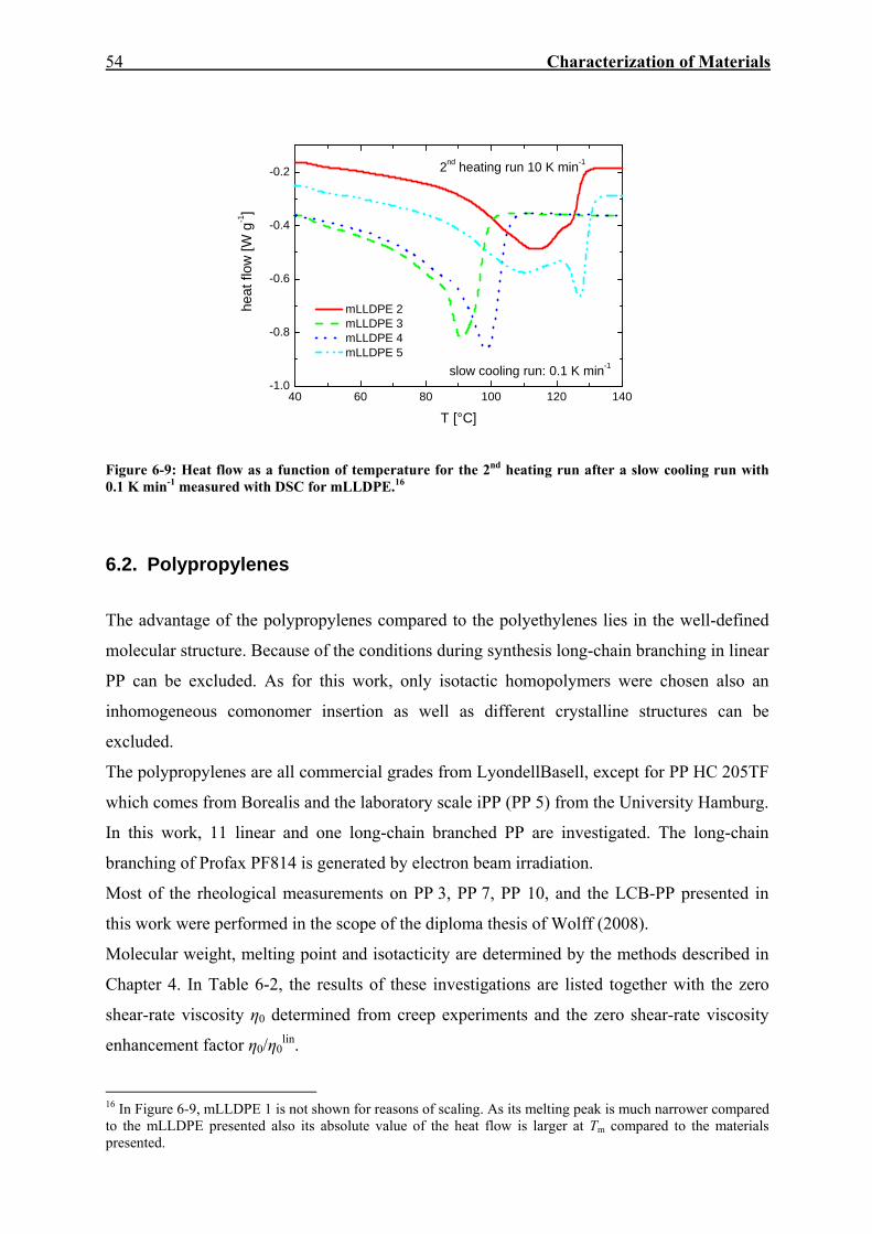
54 Characterization of Materials
40 60 80 100 120 140-1.0
-0.8
-0.6
-0.4
-0.2
heat
flow
[W g
-1]
T [°C]
mLLDPE 2 mLLDPE 3 mLLDPE 4 mLLDPE 5
2nd heating run 10 K min-1
slow cooling run: 0.1 K min-1
Figure 6-9: Heat flow as a function of temperature for the 2nd heating run after a slow cooling run with 0.1 K min-1 measured with DSC for mLLDPE.16
6.2. Polypropylenes
The advantage of the polypropylenes compared to the polyethylenes lies in the well-defined
molecular structure. Because of the conditions during synthesis long-chain branching in linear
PP can be excluded. As for this work, only isotactic homopolymers were chosen also an
inhomogeneous comonomer insertion as well as different crystalline structures can be
excluded.
The polypropylenes are all commercial grades from LyondellBasell, except for PP HC 205TF
which comes from Borealis and the laboratory scale iPP (PP 5) from the University Hamburg.
In this work, 11 linear and one long-chain branched PP are investigated. The long-chain
branching of Profax PF814 is generated by electron beam irradiation.
Most of the rheological measurements on PP 3, PP 7, PP 10, and the LCB-PP presented in
this work were performed in the scope of the diploma thesis of Wolff (2008).
Molecular weight, melting point and isotacticity are determined by the methods described in
Chapter 4. In Table 6-2, the results of these investigations are listed together with the zero
shear-rate viscosity η0 determined from creep experiments and the zero shear-rate viscosity
enhancement factor η0/η0lin.
16 In Figure 6-9, mLLDPE 1 is not shown for reasons of scaling. As its melting peak is much narrower compared to the mLLDPE presented also its absolute value of the heat flow is larger at Tm compared to the materials presented.

Characterization of Materials
55
The melting temperature Tm for the linear PP is in the range expected for isotactic PP. Only
PP 5, which was synthesized using a metallocene catalyst, has a distinctly lower Tm. In
addition, its tacticity, which is strongly linked to Tm, is the lowest compared to the other
linear PP. According to the literature stereo defects generated by the synthesis with
metallocene catalysts are responsible for disrupting the length of the crystallisable, isotactic
sequences, and thus, for lowering Tm (Phillips and Wolkowicz, 1996).
Using FT-IR-spectroscopy the PP are checked for a possible content of comonomer. As for
none of these materials characteristic peaks for ethylene-propylene copolymers at
wavenumbers between 700 and 750 cm-1 are found it is assumed that all PP investigated are
homopolymers.
Considering the accuracy of the method the isotacticity for most of the linear PP can be
regarded as 100%. Only PP 2, PP 5, and PP 9 have somewhat smaller isotacticities.17
The LCB-PP 1 shows a distinctly smaller isotacticity. This result and the presence of long-
chain branches are responsible for the lower melting point compared to the linear PP (Stange,
2006).
Table 6-2: Molecular and rheological characteristics of PP.
Commercial name Designation Mw Mw/Mn Tm Isotacticity η0 (T = 180°C) η0/η0
lin
[kg mol-1] [-] [°C] [%] [Pa s] [-]
Linear PP
Novolen 1100 RC PP 1 192 4.0 162.9 100±2 1240±10 1.00
Moplen HP 500N PP 2 244 3.5 162.9 93±2 2730±50 0.96
Moplen HP 501N PP 3 254 6.0 165.4 101±2 3340±10 1.01
Moplen HP510M PP 4 263 6.4 164.9 100±2 4690±100 1.26
iPP Hamburg PP 5 265 2.5 154.5 95±2 4170±310 1.09
Novolen 1100N PP 6 268 7.7 166.2 100±2 4000±20 1.01
Moplen HP 501L PP 7 325 5.9 164.9 99±2 7650±250 0.98
PP HC 205TF PP 8 342 5.8 165.0 99±2 11 400±50 1.22
Moplen HP 501H PP 9 376 4.7 163.4 96±2 16 700±100 1.29
Moplen HP 556E PP 10 525 6.0 164.6 99±2 48 700±1000 1.17
Daplen BE 50 PP 11 738 6.0 164.9 98±2 168 000±20 000 1.22
LCB-PP
Profax PF 814 LCB-PP 1067 22 159.6 93±2 52 000±2000 0.10
17 The reason for the smaller isotacticity of PP 2 and PP 5 could be a small ethylene content not detectable from the IR-spectrum.

56 Characterization of Materials
The weight average molar masses Mw and polydispesities Mw/Mn given in Table 6-2 are
determined by SEC-MALLS. The molar mass distributions (MMD) of PP 1, PP 2, PP 3, PP 4,
PP 5, and PP 6 are presented in Figure 6-10, those of PP 7, PP 8, PP 9, PP 10, PP 11, and
LCB-PP in Figure 6-11. All linear PP have a quite symmetric MMD. The LCB-PP, however,
shows a broader distribution with high molecular weight components.
104 105 106 1070.0
0.2
0.4
0.6
0.8
1.0
1.2
1.4 1,2,4-TCBT = 140°C
0.5 ml min-1
dW/d
(log(
M))
[-]
Mw,LS [g mol-1]
PP 1 PP 2 PP 3 PP 4 PP 5 PP 6
Figure 6-10: Molar mass distributions of PP 1, PP 2, PP 3, PP 4, PP 5, and PP 6.
104 105 106 1070.0
0.2
0.4
0.6
0.8
1.0
1.2
1.4 1,2,4-TCBT = 140°C
0.5 ml min-1
dW/d
(log(
M))
[-]
Mw,LS [g mol-1]
PP 7 PP 8 PP 9 PP 10 PP 11 LCB-PP
Figure 6-11: Molar mass distributions of PP 7, PP 8, PP 9, PP 10, PP 11, and LCB-PP.
The results of the analysis of the mean square value of the radius of gyration <rg2>0.5 versus
the absolute molar mass Mw,LS is shown exemplarily for PP 1, PP 9, and LCB-PP in Figure
6-12 and for PP 5 (metallocene type) and PP 7 in Figure 6-13. The radii of gyration of the

Characterization of Materials
57
linear PP come to lie on the reference line for linear PP with a slope of 0.585. The LCB-PP
shows a very pronounced coil contraction similar to the behaviour of the LDPE.18
105 106 10710
100
1,2,4-TCBT = 140°C
0.5 ml min-1
PP 1 PP 9 LCB-PP
<r2 g>0.
5 [nm
]
Mw,LS [g mol-1]
linear PP
Figure 6-12: Mean square value of the radius of gyration <rg
2>0.5 as a function of the absolute molar mass Mw,LS for PP 1, PP 9, and LCB-PP.
105 106 10710
100
1,2,4-TCBT = 140°C
0.5 ml min-1
PP 5 PP 7
<r2 g>0.
5 [nm
]
Mw,LS [g mol-1]
linear PP
Figure 6-13: Mean square value of the radius of gyration <rg
2>0.5 as a function of the absolute molar mass Mw,LS for PP 5 and PP 7. The values for the zero shear-rate viscosity η0 listed in Table 6-2 are determined from creep
experiments in the linear stress regime (see Chapter 5.1.3). They are average values from at
least four measurements. They can be related to the absolute weight average molar mass
18 As for the LDPE, the radii of gyration of the LCB-PP are truncated at molar masses below 300 000 g mol-1 as indications for non-ideal separation in the SEC become visible.

58 Characterization of Materials
Mw,LS according to Equation (3.2). The relationship for the linear polypropylenes described by
η0lin = 3.98·10-16·Mw,LS
3.5 is taken from Auhl et al. (2004). The value of η0/η0lin for all linear
PP is around one, and thus, the absence of long-chain branching is confirmed. The η0 for the
LCB-PP lies below the relationship for linear PP, therefore, a treelike branching structure can
be expected (Auhl et al., 2004).
102 103102
103
104
105
106
107
PP 7 PP 8 PP 9 PP 10 PP 11 LCP-PP
ηlin0 = 3.98×10⁻¹⁶×Mw,LS
3.5
PP 1 PP 2 PP 3 PP 4 PP 5 PP 6
η 0 [Pa
s]
Mw,LS [g mol-1]
T = 180°C
(Auhl et al., 2004)
Linear PP
Figure 6-14: Zero shear-rate viscosity η0 as a function of the absolute molar mass Mw,LS for all PP investigated.
Rheological Measurements in Shear
59
7. Rheological Measurements in Shear
7.1. Dynamic-Mechanical Experiments
The results of dynamic-mechanical experiments are typically presented as G´ and G´´ as a
function of the angular frequency ω. Van Gurp and Palmen (1998) proposed the plot of the
phase angle δ as a function of the complex modulus |G*| as a tool to detect thermorheological
complexity. The δ(|G*|)-plot is very sensitive with respect to long-chain branching but is also
influenced by the molar mass distribution (van Gurp and Palmen, 1998, Trinkle and Friedrich,
2001, Trinkle et al., 2002). For thermorheologically simple polymer melts, no dependence of
δ vs. |G*| on temperature is found while a thermorheological complexity leads to a
temperature dependence of the shape of δ vs. |G*| (van Gurp and Palmen, 1998).
The zero shear-rate enhancement factor η0/η0lin and the behaviour in the δ(|G*|)-plot were
chosen as the criteria for the determination of LCB. Furthermore, the δ(|G*|)-plot is used for
the detection of thermorheological complexity (e.g. Stadler, 2007).
In Figure 7-1, the δ(|G*|)-plots for one linear mLLDPE (mLLDPE 2), one LCB-mLLDPE
(LCB-mLLDPE 3), and one LDPE (LDPE-tub 4) are presented. The materials chosen are
representative for each material class. The curves of the linear material measured at four
different temperatures coincide, whereas the samples containing long-chain branches show a
deviation in the shape of the curves. Additionally, the curves for the different temperatures
split up.
The curves for the LCB-mLLDPE approach at low and high phase angles δ the curves of the
linear material. In the middle range of phase angles, the curves show a deflection point and
split up systematically for the different temperatures. This behaviour is typical of LCB-
mLLDPE and also reported in the literature (e.g. Stadler, 2007).
For the LDPE the deviation from the linear material is even more pronounced. The curves for
the different temperatures split up in the whole range of phase angles measured. However, for
this material class no deflection point is found.

60 Rheological Measurements in Shear
102 103 104 105 106
20
30
40
50
60
70
80
90
δ [°
]
IG*I [Pa]
LDPE-tub 4 130°C 150°C 170°C 190°C
mLLDPE 2 130°C 150°C 170°C 190°C
LCB-mLLDPE 3 130°C 150°C 170°C 190°C
Figure 7-1: δ(|G*|)-plots for mLLDPE 2, LCB-mLLDPE 3, and LDPE-tub 4 at 130, 150, 170, and 190°C.
In Figure 7-2, the δ(|G*|)-plots of all mLLDPE and LCB-mLLPDE are presented at 170°C.
For all linear materials, the plots coincide over a wide range of |G*|. The coincidence at high
|G*| is a bit poorer because of experimental limitations. When taking a closer look at the data
of mLLDPE 3, small deviations from the behaviour of the other linear materials occur in the
range of |G*| from 1000 to 10 000 Pa. This observation provides a small hint to
thermorheological complexity because this deviation also occurs for all other temperatures
and increases with decreasing temperature leading to a systematic split up, as presented in
Appendix 12.3 in Figure 12-9. 19 For the mLLDPE 4, such a hint to thermorheological
complexity is not seen, although it is expected from the analysis of the temperature
dependence of Je0 (see Chapter 7.2.3).
Concerning the δ(|G*|)-plots of the LCB-mLLDPE (Figure 7-2), LCB-mLLDPE 1 shows the
strongest deviation from the linear reference and differs significantly from the behaviour of
the other LCB-mLLDPE. Therefore, for LCB-mLLDPE 1 a different branching structure
compared to LCB-mLLDPE 2, LCB-mLLDPE 3, or LCB-mLLDPE 4 is presumable.
19 The δ|G*|-plots of mLLDPE 3 and mLLDPE 4 at four measuring temperatures are given in Appendix 12.3.

Rheological Measurements in Shear
61
102 103 104 105 106
30
40
50
60
70
80
90 T = 170°C
δ [°
]
IG*I [Pa]
mLLDPE mLLDPE 1 mLLDPE 2 mLLDPE 3 mLLDPE 4 mLLDPE 5
LCB-mLLDPE LCB-mLLDPE 1 LCB-mLLDPE 2 LCB-mLLDPE 3 LCB-mLLDPE 4
Figure 7-2: δ(|G*|)-plots for different mLLDPE and LCB-mLLDPE at 170°C.
In Figure 7-3, the δ(|G*|)-plots for all LDPE are given. The δ(|G*|)-plots of LDPE-tub 1 and
LDPE-aut 1, having the lowest Mw and Mw/Mn, lie closer to the linear reference than the other
LDPE. Between these two LDPE no significant differences in the shape of δ(|G*|) are
noticeable. This corresponds to the results of branching analysis where no differences in the
plot of <rg2>0.5 as function of Mw,LS are distinguishable (see Figure 6-6).
The shape of δ(|G*|) is similar for LDPE-tub 2, LDPE-tub 3, and LDPE-tub 4. However, the
higher Mw the more δ(|G*|) shifts towards lower δ and higher |G*|. The comparison of
δ(|G*|) for LDPE-tub 4 and LDPE-aut 2, having both similar Mw and Mw/Mn, shows that
δ(|G*|) of the autoclave product is only similar to the tubular LDPE-tub 4 at the highest |G*|.
With decreasing |G*|, δ of LDPE-aut 2 increases more strongly and reaches values of δ in the
range of LDPE-tub 2 at higher |G*|. This behaviour is also reflected in <rg2>0.5 vs. Mw,LS
presented in Figure 6-7. Small differences between LDPE-tub 4 and LDPE-aut 2 are detected.
The δ|G*|-plots of various linear PP (PP 2, PP 5, PP 6, PP 8, and PP 9) having different
polydispersities and of the LCB-PP are presented in Figure 7-4.
The influence of MMD on δ as a function of |G*| can be studied from the linear PP. In
accordance to the literature (Trinkle and Friedrich, 2001) it is observed that the higher Mw/Mn
the stronger δ(|G*|) shifts towards lower |G*| and lower δ. δ(|G*|) for the LCB-PP differs
from the behaviour of the linear PP and resembles that of the LDPE.

62 Rheological Measurements in Shear
102 103 104 105 10620
30
40
50
60
70
80
90
δ [°
]
IG*I [Pa]
LDPE-tub 1 LDPE-tub 2 LDPE-tub 3 LDPE-tub 4 LDPE-aut 1 LDPE-aut 2
linear reference
T = 170°C
Figure 7-3: δ(|G*|)-plots for different LDPE at 170°C.
101 102 103 104 105
20
40
60
80
PP 6 Mw/Mn= 7.7 PP 8 Mw/Mn= 5.8 PP 9 Mw/Mn= 4.7 LCB-PP Mw/Mn= 22
PP 2 Mw/Mn= 3.5 PP 5 Mw/Mn= 2.5
δ [°
]
IG*I [Pa]
T = 180°C
Figure 7-4: δ(|G*|)-plots for various linear PP and the LCB-PP at 180°C.

Rheological Measurements in Shear
63
7.2. Creep-Recovery Experiments
From the creep-recovery experiments in shear the shear compliance J(t) and the recoverable
compliance Jr(tr) are determined. Additionally, for measurements performed until the steady
state the determination of the stationary viscosity η and the steady-state elastic compliance Je
is possible. In the linear stress regime, the measured quantities are the zero shear-rate
viscosity η0 and the linear steady-state elastic compliance Je0. These rheological quantities are
discussed in the following chapters.
7.2.1. Linear Viscous Properties
This chapter presents the discussion of the shear compliance J(t) and the zero shear-rate
viscosity η0 as a function of molecular structure.
• Analysis of the shape of J(t)
The creep curves J(t) are not only of interest for the determination of η0 but also their shape
reflects the relaxation processes of the materials. However, these processes cannot be
ascribed unambiguously to features of the molecular structure. Comparing J(t) for the
different material classes, as can be seen for the PE from Figure 7-5, Figure 7-6, and Figure
7-7, LCB-mLLDPE and LDPE require much longer creep times to reach the steady-state
regime where J(t) has the double-logarithmic slope of 1.
The J(t) of mLLDPE 2, mLLDPE 3, mLLDPE 4, and mLLDPE 5 (Figure 7-5) cannot be
distinguished. This is on the one hand due to the similar Mw of the materials that is also
responsible for the similar η0 and on the other hand due to the similar Mw/Mn that would also
change the shape of the curves, especially in the short time regime. The significantly smaller
Mw of mLLDPE 1 is also reflected in J(t) as it lies higher than the curves of the other
mLLDPE.

64 Rheological Measurements in Shear
0.1 1 10 10010-5
10-4
10-3
10-2
mLLDPE 1 mLLDPE 2 mLLDPE 3 mLLDPE 4 mLLDPE 5
J(t)
[Pa-1
]
t [s]
T = 170°C
1
Figure 7-5: J(t) for various linear mLLDPE at 170°C measured in the linear regime.
J(t) of LCB-mLLDPE 3 and LCB-mLLDPE 4 are very similar; only at longer creep times
LCB-mLLDPE 4 deviates towards higher J(t). As these materials have similar Mw and Mw/Mn
and are, furthermore, produced by the same technology this result is not surprising.
J(t) of LCB-mLLPDE 2 lies at short creep times similar to J(t) of LCB-mLLPDE 1 and runs
over the whole time range approximately parallel to J(t) of LCB-mLLDPE 3 and LCB-
mLLDPE 4. Only J(t) of LCB-mLLDPE 1 shows a curvature significantly different from the
other LCB-mLLDPE. This is a hint that the molecular structure of this material differs from
that of the other LCB-mLLDPE. These differences also are reflected in the plot of δ as a
function of |G*| where the strongest deviation from the linear reference is found for LCB-
mLLDPE 1 (see Figure 7-2). The activation energy Ea is the highest for LCB-mLLDPE 1, too
(see Table 7-1).
J(t) of the LDPE are presented in Figure 7-7. Concerning this type of materials the
differences between tubular and autoclave LDPE seem to be interesting. LDPE-tub 1 and
LDPE-aut 1 have similar Mw. J(t) of these materials run in parallel, however, J(t) of LDPE-
tub 1 lies at a higher level which also involves a significantly lower η0. Also LDPE-tub 4 and
LDPE-aut 2 have similar Mw. J(t) for these materials is the same up to 20 s but then LDPE-
aut 2 deviates towards a higher J(t) that leads to a lower η0. The analysis of J(t) shows a
significant difference between LDPE-tub 1 and LDPE-aut 1 despite the simlar Mw of the two
materials. This difference is caused by the low molecular weight fraction found in the MMD
of LDPE-tub 1, which is also responsible for the low η0.
The unexpected high ratio of η0/η0lin of nearly 1 of LDPE-tub 3 is also reflected by J(t).
Despite the similar Mw and Mw/Mn of LDPE-tub 2 and LDPE-tub 3, J(t) of the latter lies much

Rheological Measurements in Shear
65
lower, presumably caused by differences in the branching architecture. These differences are
observed in the plot of <rg2>0.5 versus Mw,LS, too, where the coil contraction of LDPE-tub 2 is
more prounced at higher molar masses (see Figure 6-6 and Figure 6-7).
0.01 0.1 1 10 100 1000 10000
10-5
10-4
10-3
10-2
10-1
100
LCB-mLLDPE 1 LCB-mLLDPE 2 LCB-mLLDPE 3 LCB-mLLDPE 4
T = 170°CJ(
t) [P
a-1]
t [s]
1
Figure 7-6: J(t) for various LCB-mLLDPE at 170°C measured in the linear regime.
0.1 1 10 100 1000 1000010-5
10-4
10-3
10-2
10-1
LDPE-tub 1 LDPE-tub 2 LDPE-tub 3 LDPE-tub 4
LDPE-aut 1 LDPE-aut 2
T = 170°C
J(t)
[Pa-1
]
t [s]
1
Figure 7-7: J(t) for various LDPE at 170°C measured in the linear regime.
Figure 7-8 (a) and Figure 7-8 (b) give J(t) of the PP at 180°C. The lower Mw (the materials
are numbered according to an increasing Mw) the sooner the double-logarithmic slope of 1 is
reached. For all linear PP the curvature of J(t) is similar, only J(t) of the LCB-PP has a
different shape because of its long-chain branches.
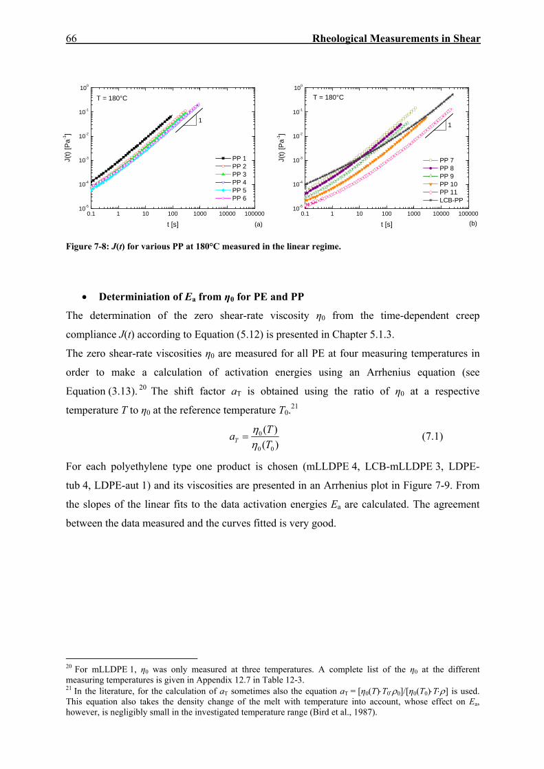
66 Rheological Measurements in Shear
Figure 7-8: J(t) for various PP at 180°C measured in the linear regime.
• Determiniation of Ea from η0 for PE and PP
The determination of the zero shear-rate viscosity η0 from the time-dependent creep
compliance J(t) according to Equation (5.12) is presented in Chapter 5.1.3.
The zero shear-rate viscosities η0 are measured for all PE at four measuring temperatures in
order to make a calculation of activation energies using an Arrhenius equation (see
Equation (3.13). 20 The shift factor aT is obtained using the ratio of η0 at a respective
temperature T to η0 at the reference temperature T0.21
)()(
00
0
TTaT η
η= (7.1)
For each polyethylene type one product is chosen (mLLDPE 4, LCB-mLLDPE 3, LDPE-
tub 4, LDPE-aut 1) and its viscosities are presented in an Arrhenius plot in Figure 7-9. From
the slopes of the linear fits to the data activation energies Ea are calculated. The agreement
between the data measured and the curves fitted is very good.
20 For mLLDPE 1, η0 was only measured at three temperatures. A complete list of the η0 at the different measuring temperatures is given in Appendix 12.7 in Table 12-3. 21 In the literature, for the calculation of aT sometimes also the equation aT = [η0(T)⋅T0⋅ρ0]/[η0(T0)⋅T⋅ρ] is used. This equation also takes the density change of the melt with temperature into account, whose effect on Ea, however, is negligibly small in the investigated temperature range (Bird et al., 1987).
0.1 1 10 100 1000 10000 10000010-5
10-4
10-3
10-2
10-1
100
PP 1 PP 2 PP 3 PP 4 PP 5 PP 6
T = 180°C
J(t)
[Pa-1
]
t [s] (a)
1
0.1 1 10 100 1000 10000 10000010-5
10-4
10-3
10-2
10-1
100
PP 7 PP 8 PP 9 PP 10 PP 11 LCB-PP
T = 180°C
J(t)
[Pa-1
]
t [s] (b)
1
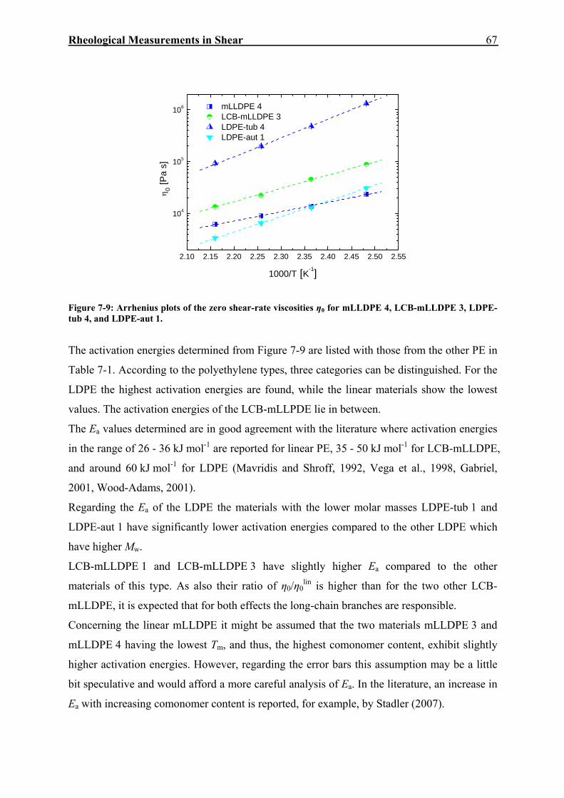
Rheological Measurements in Shear
67
2.10 2.15 2.20 2.25 2.30 2.35 2.40 2.45 2.50 2.55
104
105
106 mLLDPE 4 LCB-mLLDPE 3 LDPE-tub 4 LDPE-aut 1
η 0 [P
a s]
1000/T [K-1]
Figure 7-9: Arrhenius plots of the zero shear-rate viscosities η0 for mLLDPE 4, LCB-mLLDPE 3, LDPE-tub 4, and LDPE-aut 1.
The activation energies determined from Figure 7-9 are listed with those from the other PE in
Table 7-1. According to the polyethylene types, three categories can be distinguished. For the
LDPE the highest activation energies are found, while the linear materials show the lowest
values. The activation energies of the LCB-mLLPDE lie in between.
The Ea values determined are in good agreement with the literature where activation energies
in the range of 26 - 36 kJ mol-1 are reported for linear PE, 35 - 50 kJ mol-1 for LCB-mLLDPE,
and around 60 kJ mol-1 for LDPE (Mavridis and Shroff, 1992, Vega et al., 1998, Gabriel,
2001, Wood-Adams, 2001).
Regarding the Ea of the LDPE the materials with the lower molar masses LDPE-tub 1 and
LDPE-aut 1 have significantly lower activation energies compared to the other LDPE which
have higher Mw.
LCB-mLLDPE 1 and LCB-mLLDPE 3 have slightly higher Ea compared to the other
materials of this type. As also their ratio of η0/η0lin is higher than for the two other LCB-
mLLDPE, it is expected that for both effects the long-chain branches are responsible.
Concerning the linear mLLDPE it might be assumed that the two materials mLLDPE 3 and
mLLDPE 4 having the lowest Tm, and thus, the highest comonomer content, exhibit slightly
higher activation energies. However, regarding the error bars this assumption may be a little
bit speculative and would afford a more careful analysis of Ea. In the literature, an increase in
Ea with increasing comonomer content is reported, for example, by Stadler (2007).

68 Rheological Measurements in Shear
Table 7-1: Activation energies Ea of PE and PP determined from η0.
Material Ea [kJ mol-1] Material Ea [kJ mol-1] Material Ea [kJ mol-1] linear mLLDPE LCB-mLLDPE LDPE tubular
mLLDPE 1 30.4±3.7 LCB-mLLDPE 1 50.1±0.6 LDPE-tub 1 54.3±1.9
mLLDPE 2 33.4±1.1 LCB-mLLDPE 2 47.7±0.4 LDPE-tub 2 64.0±1.6
mLLDPE 3 35.4±0.1 LCB-mLLDPE 3 48.9±0.4 LDPE-tub 3 68.2±1.1
mLLDPE 4 34.4±0.2 LCB-mLLDPE 4 46.4±1.0 LDPE-tub 4 68.5±1.1
mLLDPE 5 32.7±0.1
LDPE autoclave linear PP*
LDPE-aut 1 57.5±0.5 PP 3 43.3±2.8
LDPE-aut 2 66.8±0.8 PP 7 41.9±1.5
PP 10 40.9±1.6
* Ea is only determined for the PP listed in this table, as the measurements at different temperatures require much effort and are not the main objective of this work.
For most of the PP η0 was only measured at 180°C, thus, for these materials (which are not
listed in Table 7-1) Ea could not be calculated.22
In Figure 7-10, the Arrhenius plots of the viscosities of PP 3, PP 7, and PP 10 are presented.
Also for these linear PP activation energies Ea can be calculated from the slopes of the linear
fits to the data.
As the activation energies Ea are determined from only three temperatures in the case of PP 3,
PP 7, and PP 10 the experimental errors are larger than for most of the PE and lie in the range
of 4 - 6%. The resulting Ea are in accordance with those found in the literature between 36
and 44 kJ mol-1 (Laun, 1987, Wassermann and Graessley, 1996, Eckstein et al., 1997, Auhl,
2006). As expected from the literature on PE (Gabriel and Münstedt, 1999) no influence of
Mw or MMD on Ea can be deduced.
22 As for the PE, a complete list of the η0 at the different measuring temperatures can be found in Appendix 12.7 in Table 12-3.

Rheological Measurements in Shear
69
2.00 2.05 2.10 2.15 2.20103
104
105
PP 3 PP 7 PP 10
η 0 [Pa
s]
1000/T [K-1]
Figure 7-10: Arrhenius plots of the zero shear-rate viscosities η0 for PP 3, PP 7, and PP 10.
7.2.2. Linear Elastic Properties
In the first section of this chapter the study of Jr(tr) should give more insight into the
correlation between elasticity and molecular architecture.
The second part of this chapter is an analysis of the influence of Mw, Mw/Mn, and long-chain
branching on the linear steady-state elastic compliance Je0 for PE and PP. Regarding the PE
especially the effects of different branching structures on Je0 are studied. The linear PP allow
the investigation of the influence of either Mw at constant Mw/Mn or of Mw/Mn at constant Mw
on Je0.
• Analysis of the shape of Jr(tr)
As for J(t), also for Jr(tr) interesting conclusions can be drawn by the analysis of the time
dependence of Jr given in Figure 7-11 for the linear mLLDPE, in Figure 7-12 for the LCB-
mLLDPE, and in Figure 7-13 for the LDPE at 170°C.23
23 In Table 7-2, the values for Je
0 are given at 150°C and also η0 (Table 6-1) and η0/η0lin are listed for this
temperature. This temperature is necessary for the comparison with the literature regarding the η0(Mw)-plot because in the literature commonly η0 values at 150°C are presented. However, the curves of Jr(tr) are shown at 170°C because later in this work most of the analyses regarding shear as well as elongational experiments are performed at 170°C. In the next chapter it is shown that Je
0 depends on temperature, and thus, also the shape of the Jr(tr) curves changes with temperature. However, as for each PE type the temperature dependence of Je
0 is similar Figure 7-11, Figure 7-12, and Figure 7-13 will not change much with temperature.

70 Rheological Measurements in Shear
From Figure 7-11 can be seen that mLLDPE 1, which has the lowest Je0 reaches the steady-
state at the shortest recovery times of about 10 s. For the other materials Je0 is reached about
one decade later.
0.1 1 10 100
10-5
10-4
mLLDPE 1 mLLDPE 2 mLLDPE 3 mLLDPE 4 mLLDPE 5
Jr(t r) [
Pa-1]
tr [s]
T = 170°C
Figure 7-11: Jr(tr) for various linear mLLDPE at 170°C measured in the linear regime.
For the LCB-mLLDPE (Figure 7-12), the recovery times necessary to reach Je0 are about
1000 s, and thus, one decade longer than for most of the mLLDPE.
As for J(t), also the course of Jr(tr) for LCB-mLLDPE 3 and LCB-mLLDPE 4 is similar. Only
at longer recovery times, the curves deviate and LCB-mLLDPE 4 reaches a higher Je0. Due to
the same production process the molecular structure of these materials can be assumed to be
very similar and following from that the similar J(t) and Jr(tr) can be understood.
The significantly different behaviour of J(t) for LCB-mLLDPE 1 and LCB-mLLDPE 2 is also
visible in Jr(tr).24 Jr(tr) of LCB-mLLDPE 1 runs at a higher level approximately parallel to
LCB-mLLDPE 3 and LCB-mLLDPE 4. Jr(tr) of LCB-mLLDPE 2 runs at short recovery
times only slightly below LCB-mLLDPE 1 but reaches a Je0 in the range of LCB-mLLDPE 3
and LCB-mLLDPE 4. This gives a hint again that the molecular structures of LCB-
mLLDPE 1 and LCB-mLLDPE 2 are different to those of LCB-mLLDPE 3 and LCB-
mLLDPE 4.
24 The similarities of J(t) and Jr(tr) at short measuring times are motivated by a comparison of Equations 5.10 and 5.15. J(t) and Jr(tr) must be the same in the time range where the viscous part of J(t) can be neglected.

Rheological Measurements in Shear
71
0.1 1 10 100 1000 1000010-5
10-4
10-3
LCB-mLLDPE 1 LCB-mLLDPE 2 LCB-mLLDPE 3 LCB-mLLDPE 4
T = 170°C
Jr(t r) [
Pa-1]
tr [s]
Figure 7-12: Jr(tr) for various LCB-mLLDPE at 170°C measured in the linear regime.
0.1 1 10 100 1000 1000010-5
10-4
10-3
LDPE-tub 1 LDPE-tub 2 LDPE-tub 3 LDPE-tub 4
LDPE-aut 1 LDPE-aut 2
Jr(t r) [
Pa-1
]
tr [s]
T = 170°C
Figure 7-13: Jr(tr) for various LDPE at 170°C measured in the linear regime.
Figure 7-13 shows that for LDPE-tub 1 and LDPE-aut 1 having lower Mw and Mw/Mn the
steady-state value Je0 is reached at recovery times of about 100 s (similar to mLLDPE),
whereas for the other LDPE recovery times of much more than 1000 s are necessary to attain
Je0.
The comparison of tubular and autoclave LDPE shows that for LDPE-tub 1 and LDPE-aut 1
having similar Mw and Mw/Mn Jr(tr) start at different levels at short recovery times but reach
similar Je0. The difference in the short time regime can be attributed to the different molar
mass distributions. The low molecular weight component of LDPE-tub 1 is responsible for
short retardation times that recover at the very beginning of the recovery experiment at

72 Rheological Measurements in Shear
measuring times smaller than 0.1 s. Thus, in Figure 7-13 at short times Jr(tr) of LDPE-tub 1
lies higher than Jr(tr) of LDPE-aut 1. For LDPE-tub 4 and LDPE-aut 2 having also similar Mw
and Mw/Mn, however, the opposite case is found; Jr(tr) are the same at short times, differ at
longer times and reach different Je0. J(t) (see Figure 7-7) of LDPE-tub 4 and LDPE-aut 2 also
differ only at long creep times. This indicates that LDPE-tub 4 and LDPE-aut 2 differ in their
molecular structures particularly concerning the molecules contributing to the long relaxation
times that determine the steady-state properties η0 and Je0.
Despite having similar Mw and Mw/Mn, J(t) (see Figure 7-7) and Jr(tr) of LDPE-tub 2 and
LDPE-tub 3 differ because of their presumably different branching structures. This is
apparent from the plot of <rg2>0.5 versus Mw,LS in Figure 6-6 and Figure 6-7 and is reflected
by the different ratios of η0/η0lin, too.
In Figure 7-14 (a) and (b), Jr(tr) of all PP at 180°C are presented. It can be seen that for all
linear PP a steady-state in Jr(tr) is reached between 100 and 1000 s; only for PP 10 and PP 11
with the highest Mw longer recovery times are necessary.
For the materials plotted in Figure 7-14 (a), the influence of polydispersity can be evaluated
independently of Mw as all PP except PP 1 have Mw of about 250 kg mol-1. The metallocene
catalyzed PP 5 with the lowest Mw/Mn also has the lowest Je0 and the level of Jr(tr) lies below
the other PP. Jr(tr) of the other PP start at the same level and according to their Mw/Mn
different steady states are reached. PP 1 has the lowest Mw of all PP. This might be the reason
for the only moderate increase of Jr(tr) from the shortest to the longest recovery times. The
same tendency is seen for PP 11 and PP 10 in Figure 7-14 (b) that have the highest Mw
(Mw/Mn ≈ 6, similar to PP 3, PP 7, and PP 8), and thus, also the increase of Jr(tr) from short to
long recovery times is the strongest.
PP 8 and PP 9 have similar Mw but different Mw/Mn of 5.8 and 4.7, respectively. Jr(tr) of PP 8
not only starts from a higher level but also increases more with recovery time and yields a
higher Je0. Je
0 of PP 7 is unexpectedly high (as discussed later). According to its Mw and
Mw/Mn a shape of Jr(tr) similar to PP 8 would be expected.
Figure 7-14 (b) also shows that the higher Mw the lower Jr(tr) at short recovery times. This
behaviour can also be seen for J(t) in Figure 7-8 (b).25 The reason for this finding is that the
short retardation times caused by the short molecules recover at short measuring times
smaller than 0.1 s. Therefore, for the materials with lower Mw the contributions of the short
molecules to Jr(tr) are already visible at short recovery times.
25 From equations 5.10 and 5.15 can be deduced that J(t) and Jr(tr) at short measuring times must be the same.
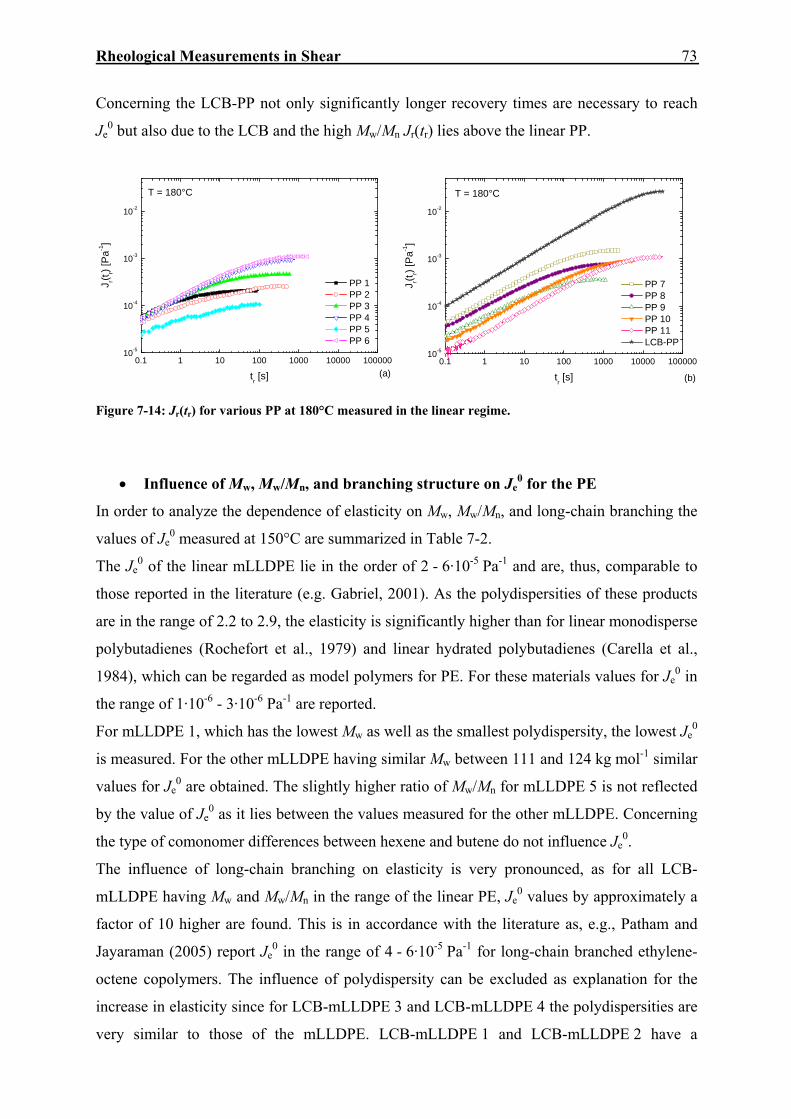
Rheological Measurements in Shear
73
Concerning the LCB-PP not only significantly longer recovery times are necessary to reach
Je0 but also due to the LCB and the high Mw/Mn Jr(tr) lies above the linear PP.
Figure 7-14: Jr(tr) for various PP at 180°C measured in the linear regime.
• Influence of Mw, Mw/Mn, and branching structure on Je0 for the PE
In order to analyze the dependence of elasticity on Mw, Mw/Mn, and long-chain branching the
values of Je0 measured at 150°C are summarized in Table 7-2.
The Je0 of the linear mLLDPE lie in the order of 2 - 6·10-5 Pa-1 and are, thus, comparable to
those reported in the literature (e.g. Gabriel, 2001). As the polydispersities of these products
are in the range of 2.2 to 2.9, the elasticity is significantly higher than for linear monodisperse
polybutadienes (Rochefort et al., 1979) and linear hydrated polybutadienes (Carella et al.,
1984), which can be regarded as model polymers for PE. For these materials values for Je0 in
the range of 1·10-6 - 3·10-6 Pa-1 are reported.
For mLLDPE 1, which has the lowest Mw as well as the smallest polydispersity, the lowest Je0
is measured. For the other mLLDPE having similar Mw between 111 and 124 kg mol-1 similar
values for Je0 are obtained. The slightly higher ratio of Mw/Mn for mLLDPE 5 is not reflected
by the value of Je0 as it lies between the values measured for the other mLLDPE. Concerning
the type of comonomer differences between hexene and butene do not influence Je0.
The influence of long-chain branching on elasticity is very pronounced, as for all LCB-
mLLDPE having Mw and Mw/Mn in the range of the linear PE, Je0 values by approximately a
factor of 10 higher are found. This is in accordance with the literature as, e.g., Patham and
Jayaraman (2005) report Je0 in the range of 4 - 6·10-5 Pa-1 for long-chain branched ethylene-
octene copolymers. The influence of polydispersity can be excluded as explanation for the
increase in elasticity since for LCB-mLLDPE 3 and LCB-mLLDPE 4 the polydispersities are
very similar to those of the mLLDPE. LCB-mLLDPE 1 and LCB-mLLDPE 2 have a
0.1 1 10 100 1000 10000 10000010-5
10-4
10-3
10-2
T = 180°C
Jr(t r) [
Pa-1]
tr [s]
PP 7 PP 8 PP 9 PP 10 PP 11 LCB-PP
(b)
0.1 1 10 100 1000 10000 10000010-5
10-4
10-3
10-2
T = 180°C
Jr(t r) [
Pa-1
]
tr [s]
PP 1 PP 2 PP 3 PP 4 PP 5 PP 6
(a)

74 Rheological Measurements in Shear
somewhat broader ratio of Mw/Mn which does not show up significantly in the elasticity,
however.
Table 7-2: Comparison of molecular data and Je
0 for the PE measured at 150°C.
Material Mw Mw/Mn Comonomer Tm Je
0 (T = 150°C)
η0/η0lin
(T = 150°C)
[kg mol-1] [-] [°C] [Pa-1] [-]
linear mLLDPE
mLLDPE 1 69 2.2 hexene* 125 (2.15±0.04)·10-5 1.00
mLLDPE 2 111 2.5 hexene* 119 (5.06±0.23)·10-5 1.18
mLLDPE 3 112 2.5 butene 93 (5.70±0.21)·10-5 1.11
mLLDPE 4 116 2.5 hexene 99 (3.35±0.10)·10-5 0.90
mLLDPE 5 124 2.9 hexene* 120 (4.63±0.52)·10-5 0.84
LCB-mLLDPE
LCB-mLLDPE 1 83 3.1 butene 79 (8.71±0.26)·10-4 7.19
LCB-mLLDPE 2 86 3.3 octene 98 (4.65±0.08)·10-4 2.81
LCB-mLLDPE 3 91 2.4 octene 106 (4.50±0.06)·10-4 7.08
LCB-mLLDPE 4 100 2.4 octene 102 (5.08±0.22)·10-4 3.68
LDPE tubular
LDPE-tub 1 150 12 - 107 (4.16±0.03)·10-4 0.05
LDPE-tub 2 217 14 - 109 (1.10±0.03)·10-3 0.41
LDPE-tub 3 278 14 - 113 (7.85±0.36)·10-4 0.97
LDPE-tub 4 377 18 - 110 (1.28±0.06)·10-3 0.45
LDPE autoclave
LDPE-aut 1 151 8.7 - 112 (3.64±0.16)·10-4 0.48
LDPE-aut 2 318 14.4 - 112 (1.01±0.44)·10-3 0.33
* The comonomer type cannot be determined using IR-spectroscopy because of the low comonomer content. The information listed here is given by the manufacturer.
The interpretation of the differences in Je0 found for the particular LCB-mLLDPE is very
difficult because of the numbers of parameters that have to be considered.
LCB-mLLDPE 3 and LCB-mLLDPE 4 are produced by the same company using the same
polymerisation technique. Thus, the branching structure can be assumed to be similar. Je0 of
LCB-mLLDPE 4 is slightly higher than that of LCB-mLLDPE 3.26 A qualitative explanation
can be derived using the results of SEC-MALLS and the findings of Graessley and Roovers
(1979) on starlike branched polystyrenes of various functionalities. For the LCB-mLLDPE
the radii of gyration come to lie on the line of the linear polyethylenes at low molar masses,
while at higher molar masses the radii are somewhat smaller than those of the linear
26 Je
0 of LCB-mLLDPE 4 is higher than Je0 of LCB-mLLDPE 3 not only at 150°C but also at the other
measuring temperatures listed in Table 7-4. Therefore, the argument of a possible measurement error is disproved.

Rheological Measurements in Shear
75
molecules (see Figure 6-5). Therefore, it can be concluded that these materials are mixtures of
linear and long-chain branched molecules with a starlike topography. Costeux et al. (2002)
assume that these materials may contain in addition a few H-shaped and more highly
branched molecules.
Graessley and Roovers observed for their starlike branched polystyrenes of fixed
functionality an increase of Je0 with molar mass. The increase of Je
0 is reflected in the
description of the molar mass dependence of Je0 for stars given by Pearson and Helfland
(1984) in Equations (3.8) and (3.9).
If the functionality of the star is fixed, an increase of molar mass results in a growing molar
mass of the arms Ma and finally in higher Je0. As in the case of LCB-mLLDPE 3 and LCB-
mLLDPE 4 the weight average molar mass of LCB-mLLDPE 4 is about 10% higher,
Equation (3.8) would predict an increase in Je0 of the same order. Comparing the values of Je
0
for these products an increase of about 12% for LCB-mLLDPE 4 is found. Therefore, the
assumption of a constant average functionality of the branching structure in LCB-mLLDPE 3
and LCB-mLLDPE 4 seems to be reasonable.
For the other materials, the long-chain branches are generated in a different production
process. Je0 of LCB-mLLDPE 2 is similar to Je
0 of LCB-mLLDPE 3, however, as Mw/Mn is
higher for LCB-mLLDPE 2, conclusions on the branching structure are difficult. For LCB-
mLLDPE 1 containing the highest amount of comonomer, the highest Je0 was measured. This
means that presumably its branching structure has to be very efficient to effect such a large
increase in Je0. According to Equation (3.8) this means that either the arm length of the
molecules Ma must be larger or the branching functionality must be lower.
The ratios of η0/η0lin are the highest for LCB-mLLDPE 1 and LCB-mLLDPE 3. The other two
products have significantly smaller ratios of η0/η0lin. Therefore, no correlation can be
established between η0/η0lin and Je
0.
The values of Je0 of the LDPE are in the range of the LCB-mLLDPE or even higher. In
comparison to the LCB-mLLDPE two molecular parameters are changed for the LDPE. First,
the molar mass distributions of the LDPE are much broader. Second, the coil contraction
measured for the LDPE (see Figure 6-6 and Figure 6-7) is much larger indicating a more
highly branched structure. For linear HDPE with similar polydispersities and Mw even higher
Je0 were reported (Gabriel, 2001).
For the LDPE with the lowest Mw and the narrowest Mw/Mn, LDPE-tub 1 and LDPE-aut 1, the
lowest Je0 are measured. It seems that Je
0 increases with increasing Mw independently of the
polymerisation technique (tubular, autoclave). This result is shown in Figure 7-15 for the
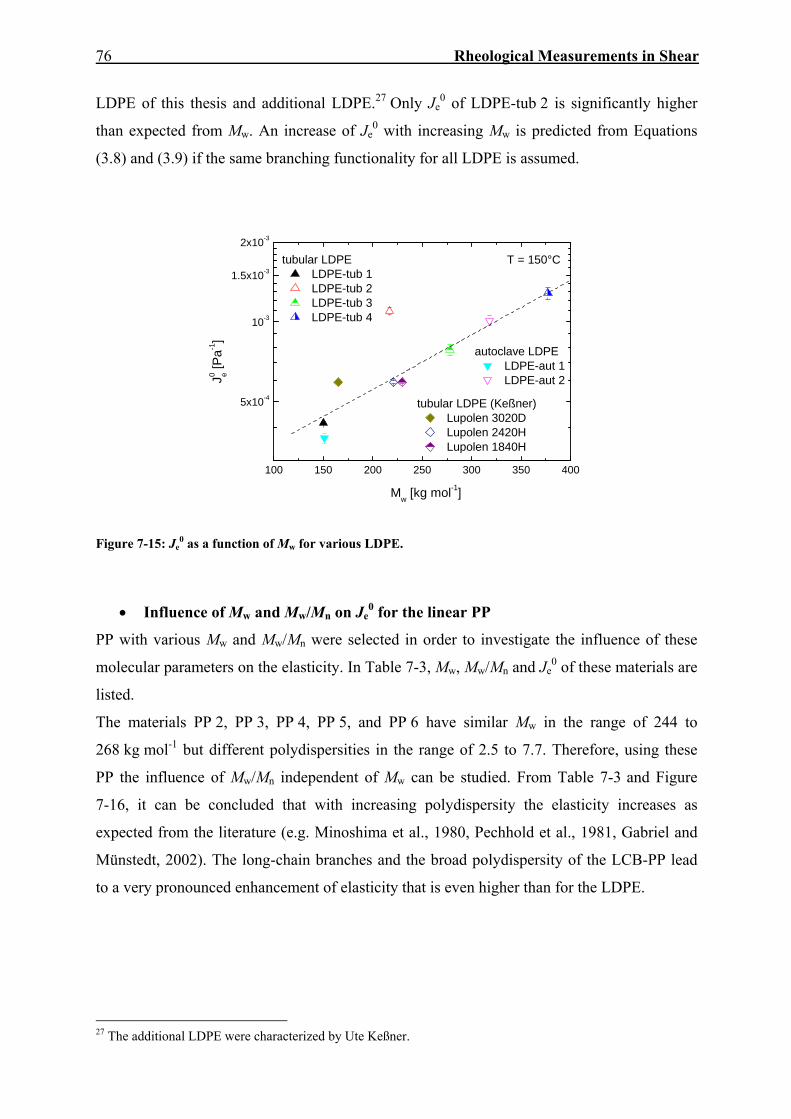
76 Rheological Measurements in Shear
LDPE of this thesis and additional LDPE.27 Only Je0 of LDPE-tub 2 is significantly higher
than expected from Mw. An increase of Je0 with increasing Mw is predicted from Equations
(3.8) and (3.9) if the same branching functionality for all LDPE is assumed.
100 150 200 250 300 350 400
5x10⁻⁴
10-3
1.5x10⁻³
2x10⁻³
autoclave LDPE LDPE-aut 1 LDPE-aut 2
tubular LDPE (Keßner) Lupolen 3020D Lupolen 2420H Lupolen 1840H
tubular LDPE LDPE-tub 1 LDPE-tub 2 LDPE-tub 3 LDPE-tub 4
J0 e [Pa-1
]
Mw [kg mol-1]
T = 150°C
Figure 7-15: Je
0 as a function of Mw for various LDPE.
• Influence of Mw and Mw/Mn on Je0 for the linear PP
PP with various Mw and Mw/Mn were selected in order to investigate the influence of these
molecular parameters on the elasticity. In Table 7-3, Mw, Mw/Mn and Je0 of these materials are
listed.
The materials PP 2, PP 3, PP 4, PP 5, and PP 6 have similar Mw in the range of 244 to
268 kg mol-1 but different polydispersities in the range of 2.5 to 7.7. Therefore, using these
PP the influence of Mw/Mn independent of Mw can be studied. From Table 7-3 and Figure
7-16, it can be concluded that with increasing polydispersity the elasticity increases as
expected from the literature (e.g. Minoshima et al., 1980, Pechhold et al., 1981, Gabriel and
Münstedt, 2002). The long-chain branches and the broad polydispersity of the LCB-PP lead
to a very pronounced enhancement of elasticity that is even higher than for the LDPE.
27 The additional LDPE were characterized by Ute Keßner.

Rheological Measurements in Shear
77
Table 7-3: Comparison of molecular data and Je0 at 180°C for PP.
Material Mw Mw/Mn Je0 (T = 180°C)
[kg mol-1] [-] [Pa-1]
linear PP
PP 1 192 4.0 (2.15±0.04)·10-4
PP 2 244 3.5 (2.66±0.09)·10-4
PP 3 254 6.0 (4.52±0.11)·10-4
PP 4 263 6.4 (9.32±0.09)·10-4
PP 5 265 2.5 (1.01±0.06)·10-4
PP 6 268 7.7 (1.21±0.01)·10-3
PP 7 325 5.9 (1.55±0.38)·10-3
PP 8 342 5.8 (7.47±0.08)·10-4
PP 9 376 4.7 (3.68±0.05)·10-4
PP 10 525 6.0 (9.08±0.15)·10-4
PP 11 738 6.0 (1.15±0.10)·10-3
LCB-PP
LCB-PP 1067 22 (2.66±0.09)·10-2
Regarding the materials PP 7, PP 8, and PP 9 having Mw between 325 and 376 kg mol-1 the
material PP 9 with the lowest Mw/Mn also exhibits the lowest Je0. The two other materials
PP 7 and PP 8 have nearly the same polydispersity of 5.9 and 5.8, respectively, the values of
Je0, however, are different. PP 7 shows the highest elasticity of all materials investigated. One
reason could be a high molar mass component or differences of the tacticity. From special
SEC measurements, DSC measurements, and a temperature rising elution fractionation
analysis (TREF), a high molar mass component or an atactic fraction can be excluded (see
Appendix 12.8).
3 4 5 6 7 8
10-4
10-3≈
PP 2 PP 3 PP 4 PP 5 PP 6
J0 e [Pa-1
]
Mw/Mn [-]
T = 180°CMw 250 kg mol-1
Figure 7-16: Influence of polydispersity Mw/Mn on Je
0 for linear PP with similar molar masses Mw in the range of 244 - 269 kg mol-1.
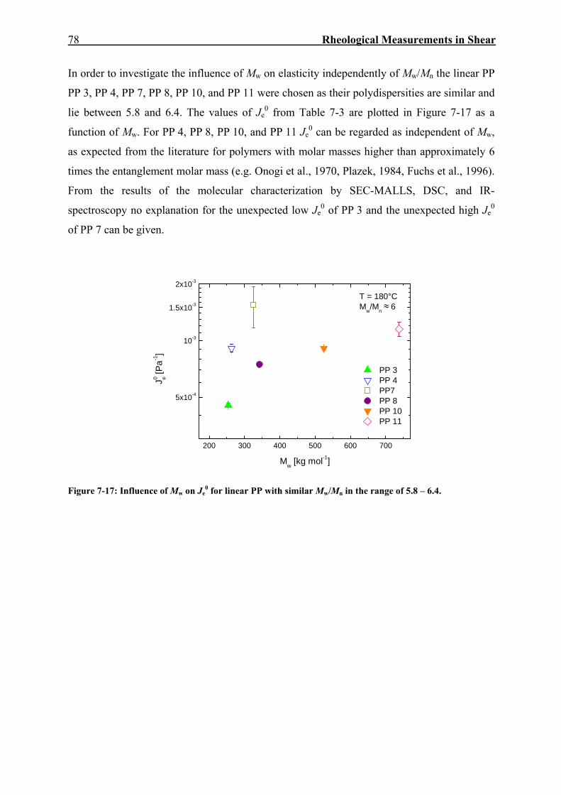
78 Rheological Measurements in Shear
In order to investigate the influence of Mw on elasticity independently of Mw/Mn the linear PP
PP 3, PP 4, PP 7, PP 8, PP 10, and PP 11 were chosen as their polydispersities are similar and
lie between 5.8 and 6.4. The values of Je0 from Table 7-3 are plotted in Figure 7-17 as a
function of Mw. For PP 4, PP 8, PP 10, and PP 11 Je0 can be regarded as independent of Mw,
as expected from the literature for polymers with molar masses higher than approximately 6
times the entanglement molar mass (e.g. Onogi et al., 1970, Plazek, 1984, Fuchs et al., 1996).
From the results of the molecular characterization by SEC-MALLS, DSC, and IR-
spectroscopy no explanation for the unexpected low Je0 of PP 3 and the unexpected high Je
0
of PP 7 can be given.
200 300 400 500 600 700
5x10⁻⁴
10-3
1.5x10⁻³
2x10⁻³
≈
PP 3 PP 4 PP7 PP 8 PP 10 PP 11
J0 e [Pa-1
]
Mw [kg mol-1]
T = 180°CMw/Mn 6
Figure 7-17: Influence of Mw on Je
0 for linear PP with similar Mw/Mn in the range of 5.8 – 6.4.
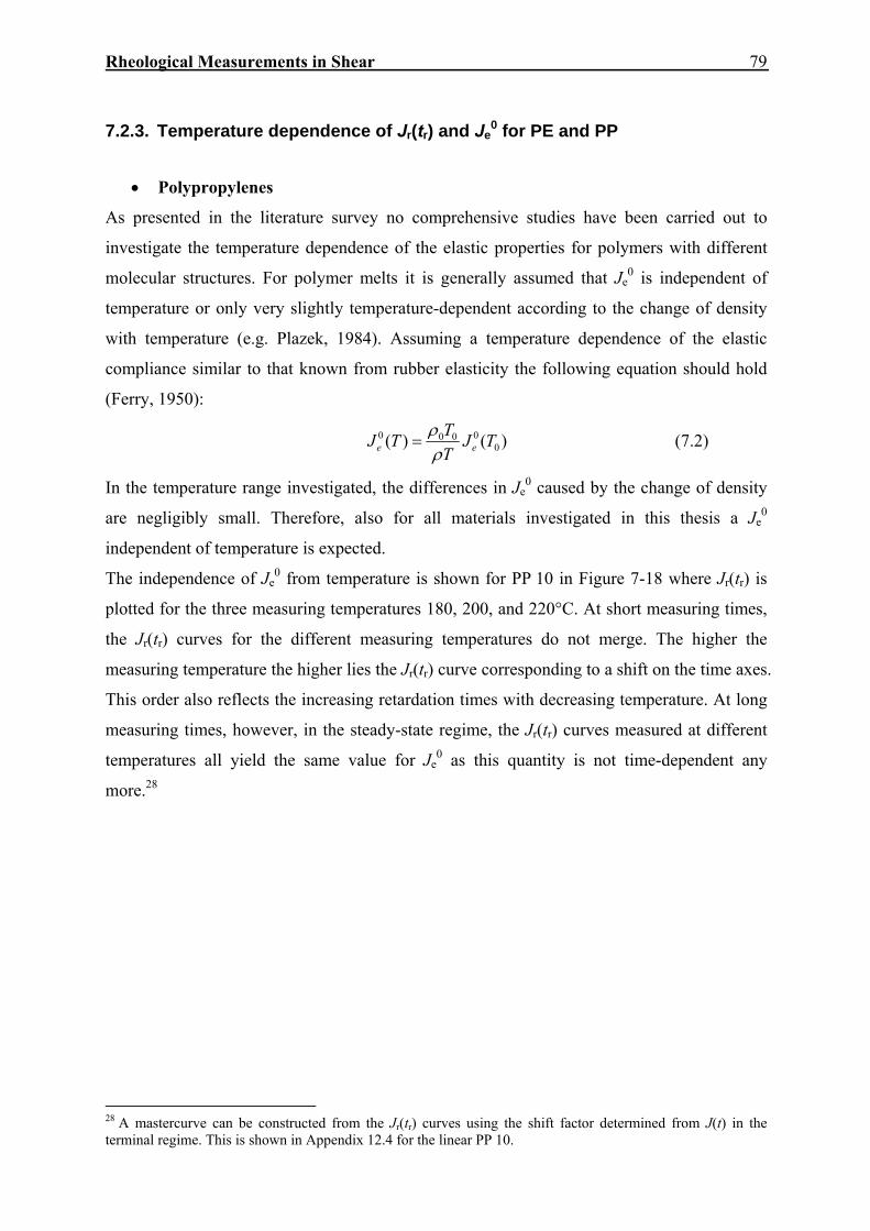
Rheological Measurements in Shear
79
7.2.3. Temperature dependence of Jr(tr) and Je0 for PE and PP
• Polypropylenes
As presented in the literature survey no comprehensive studies have been carried out to
investigate the temperature dependence of the elastic properties for polymers with different
molecular structures. For polymer melts it is generally assumed that Je0 is independent of
temperature or only very slightly temperature-dependent according to the change of density
with temperature (e.g. Plazek, 1984). Assuming a temperature dependence of the elastic
compliance similar to that known from rubber elasticity the following equation should hold
(Ferry, 1950):
)()( 00000 TJ
TTTJ ee ρ
ρ= (7.2)
In the temperature range investigated, the differences in Je0 caused by the change of density
are negligibly small. Therefore, also for all materials investigated in this thesis a Je0
independent of temperature is expected.
The independence of Je0 from temperature is shown for PP 10 in Figure 7-18 where Jr(tr) is
plotted for the three measuring temperatures 180, 200, and 220°C. At short measuring times,
the Jr(tr) curves for the different measuring temperatures do not merge. The higher the
measuring temperature the higher lies the Jr(tr) curve corresponding to a shift on the time axes.
This order also reflects the increasing retardation times with decreasing temperature. At long
measuring times, however, in the steady-state regime, the Jr(tr) curves measured at different
temperatures all yield the same value for Je0 as this quantity is not time-dependent any
more.28
28 A mastercurve can be constructed from the Jr(tr) curves using the shift factor determined from J(t) in the terminal regime. This is shown in Appendix 12.4 for the linear PP 10.
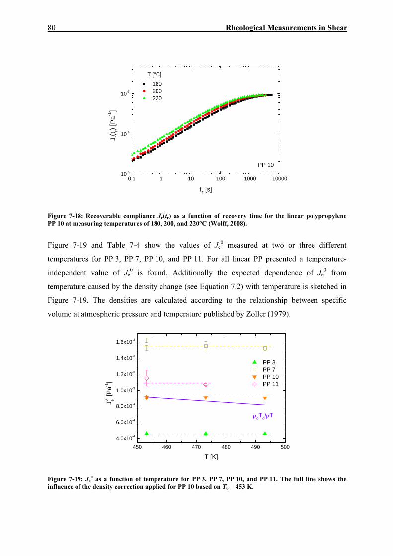
80 Rheological Measurements in Shear
0.1 1 10 100 1000 1000010-5
10-4
10-3
180 200 220
J r(tr)
[Pa-1
]
tr [s]
PP 10
T [°C]
Figure 7-18: Recoverable compliance Jr(tr) as a function of recovery time for the linear polypropylene PP 10 at measuring temperatures of 180, 200, and 220°C (Wolff, 2008).
Figure 7-19 and Table 7-4 show the values of Je0 measured at two or three different
temperatures for PP 3, PP 7, PP 10, and PP 11. For all linear PP presented a temperature-
independent value of Je0 is found. Additionally the expected dependence of Je
0 from
temperature caused by the density change (see Equation 7.2) with temperature is sketched in
Figure 7-19. The densities are calculated according to the relationship between specific
volume at atmospheric pressure and temperature published by Zoller (1979).
450 460 470 480 490 5004.0x10-4
6.0x10⁻⁴
8.0x10⁻⁴
1.0x10⁻³
1.2x10⁻³
1.4x10⁻³
1.6x10⁻³
ρ0T0/ρT
PP 3 PP 7 PP 10 PP 11
J0 e [Pa
-1]
T [K]
Figure 7-19: Je
0 as a function of temperature for PP 3, PP 7, PP 10, and PP 11. The full line shows the influence of the density correction applied for PP 10 based on T0 = 453 K.

Rheological Measurements in Shear
81
Table 7-4: Linear steady-state elastic compliance Je0 of PE and PP at various measuring temperatures.*
Material Je0 at 130°C [Pa-1] Je
0 at 150°C [Pa-1] Je0 at 170°C [Pa-1] Je
0 at 190°C [Pa-1]
mLLDPE
mLLDPE 1 n.d.** (2.15±0.04)·10-5 (2.05±0.04)·10-5 (1.97±0.07)·10-5
mLLDPE 2 (5.03±0.13)·10-5 (5.06±0.23)·10-5 (5.05±0.22)·10-5 (4.98±0.17)·10-5
mLLDPE 3 (6.55±0.34)·10-5 (5.70±0.21)·10-5 (5.28±0.20)·10-5 (4.79±0.14)·10-5
mLLDPE 4 (3.64±0.09)·10-5 (3.35±0.10)·10-5 (2.96±0.04)·10-5 (2.61±0.04)·10-5
mLLDPE 5 (4.60±0.08)·10-5 (4.63±0.52)·10-5 (4.55±0.23)·10-5 (4.57±0.30)·10-5
LCB-mLLDPE
LCB-mLLDPE 1 (9.78±0.20)·10-4 (8.71±0.25)·10-4 (7.66±0.12)·10-4 (6.66±0.17)·10-4
LCB-mLLDPE 2 (5.57±0.13)·10-4 (4.65±0.08)·10-4 (4.22±0.04)·10-4 (3.78±0.05)·10-4
LCB-mLLDPE 3 (5.14±0.09)·10-4 (4.50±0.06)·10-4 (3.98±0.06)·10-4 (3.55±0.03)·10-4
LCB-mLLDPE 4 (5.95±0.37)·10-4 (5.08±0.22)·10-4 (4.38±0.06)·10-4 (3.82±0.11)·10-4
LDPE tubular
LDPE-tub 1 (4.73±0.03)·10-4 (4.16±0.03)·10-4 (3.74±0.05)·10-4 (3.35±0.04)·10-4
LDPE-tub 2 (1.17±0.06)·10-3 (1.10±0.03)·10-3 (1.03±0.07)·10-3 (9.75±0.40)·10-4
LDPE-tub 3 (9.01±0.46)·10-4 (7.85±0.36)·10-4 (6.88±0.39)·10-4 (6.04±0.16)·10-4
LDPE-tub 4 (1.41±0.01)·10-3 (1.28±0.06)·10-3 (1.19±0.04)·10-3 (1.03±0.09)·10-3
LDPE autoclave
LDPE-aut 1 (4.13±0.08)·10-4 (3.64±0.16)·10-4 (3.35±0.06)·10-4 (3.05±0.23)·10-4
LDPE-aut 2 (1.11±0.01)·10-3 (1.01±0.04)·10-3 (8.85±0.05)·10-4 (7.75±0.27)·10-4
Je0 at 180°C [Pa-1] Je
0 at 200°C [Pa-1] Je0 at 220°C [Pa-1]
linear PP***
PP 3 (4.52±0.11)·10-4 (4.53±0.21)·10-4 (4.52±0.14)·10-4
PP 7 (1.55±0.05)·10-3 (1.57±0.08)·10-3 (1.52±0.03)·10-3
PP 10 (9.08±0.09)·10-4 (9.10±0.15)·10-4 (9.05±0.08)·10-4
PP 11 (1.15±0.10)·10-3 (1.07±0.01)·10-3 n.d.
* The Je0 values presented are average values from at least four measurements.
** Because of the high melting temperature Tm η0 at 130°C could not be determined. *** For the linear PP not listed, Je
0 was only determined at 180°C (see Table 7-3).
• Polyethylenes
Concering the PE from Table 7-4 can be seen that for the thermorheological complex LCB-
mLLDPE Je0 exhibits a pronounced temperature dependence. From the lowest to the highest
measuring temperature, Je0 decreases by about 50%. In Figure 7-20, Jr(tr) and J(t) are plotted
for the LCB-mLLDPE 3 at the four measuring temperatures 130, 150, 170, and 190°C. At
short times where the viscous contribution to J(t) is still negligible Jr(tr) and J(t) are nearly
identical. In contrast to the linear PP (see Figure 7-18) the curves of Jr(tr) for the different
temperatures cross each other and reach different stationary values of Je0.

82 Rheological Measurements in Shear
10-1 100 101 102 103 10410-5
10-4
10-3
10-2
10-1
100
J
J(t),
Jr(t
r) [P
a-1]
t, tr [s]
130°C 150°C 170°C 190°C
Jr T
LCB-mLLDPE 3
Figure 7-20: Creep compliance J(t) and recoverable compliance Jr(tr) as a function of creep and recovery time for LCB-mLLDPE 3 at measuring temperatures of 130, 150, 170, and 190°C.
In Figure 7-21, the steady-state recoverable compliance Je0 is semi-logarithmically plotted as
a function of the inverse absolute temperature for all LCB-mLLDPE investigated.29
2.1 2.2 2.3 2.4 2.5
4x10⁻⁴
6x10⁻⁴
8x10⁻⁴
10-3
LCB-mLLDPE 1 LCB-mLLDPE 2 LCB-mLLDPE 3 LCB-mLLDPE 4
ρ0T0/ρT
J0 e [P
a-1]
1000/T [K-1]
Figure 7-21: Je
0 as a function of the inverse absolute temperature for LCB-mLLDPE 1, LCB-mLLDPE 2, LCB-mLLDPE 3, and LCB-mLLDPE 4. The full line shows the influence of the density correction applied for LCB-mLLDPE 1 based on T0 = 403 K.
29 The plot of Je
0 as a function of the inverse absolute temperature would allow a determination of “apparent” activation energies (Keßner et al., 2009). However, the molecular processes responsible for the “apparent” activation energies are still unclear. Therefore, they are not reported.

Rheological Measurements in Shear
83
As can be seen from Table 7-4, also for the LDPE temperature-dependent Je0 are detected. In
Figure 7-22, Jr(tr) of the LDPE-tub 4 are plotted in a semi-logarithmic scale in order to make
the differences between the different temperatures clearer. As for the LCB-mLLDPE, the
Jr(tr) curves cross each other and reach different terminal values.
10-1 100 101 102 103 104 1050.0
0.2
0.4
0.6
0.8
1.0
1.2
1.4
1.6
Jr(t
r) [10
-3 Pa
-1]
tr [s]
130°C 150°C 170°C 190°C
LDPE-tub 4
Jr T
Figure 7-22: Recoverable compliance Jr(tr) as a function of recovery time for the LDPE-tub 4 at measuring temperatures of 130, 150, 170, and 190°C.
In Figure 7-23, the linear steady-state elastic compliances Je0 are plotted as a function of the
inverse absolute temperature for all the LDPE investigated. The Je0 of the LDPE show a
weaker temperature dependence than the LCB-mLLDPE. Linear fits are applied to the data of
Je0. The slopes of these fits are similar for all LDPE except for LDPE-tub 2, which exhibits a
less pronounced temperature dependence of Je0. This material is also the only one that
deviates from the relationship Je0 vs. Mw presented in Figure 7-15.
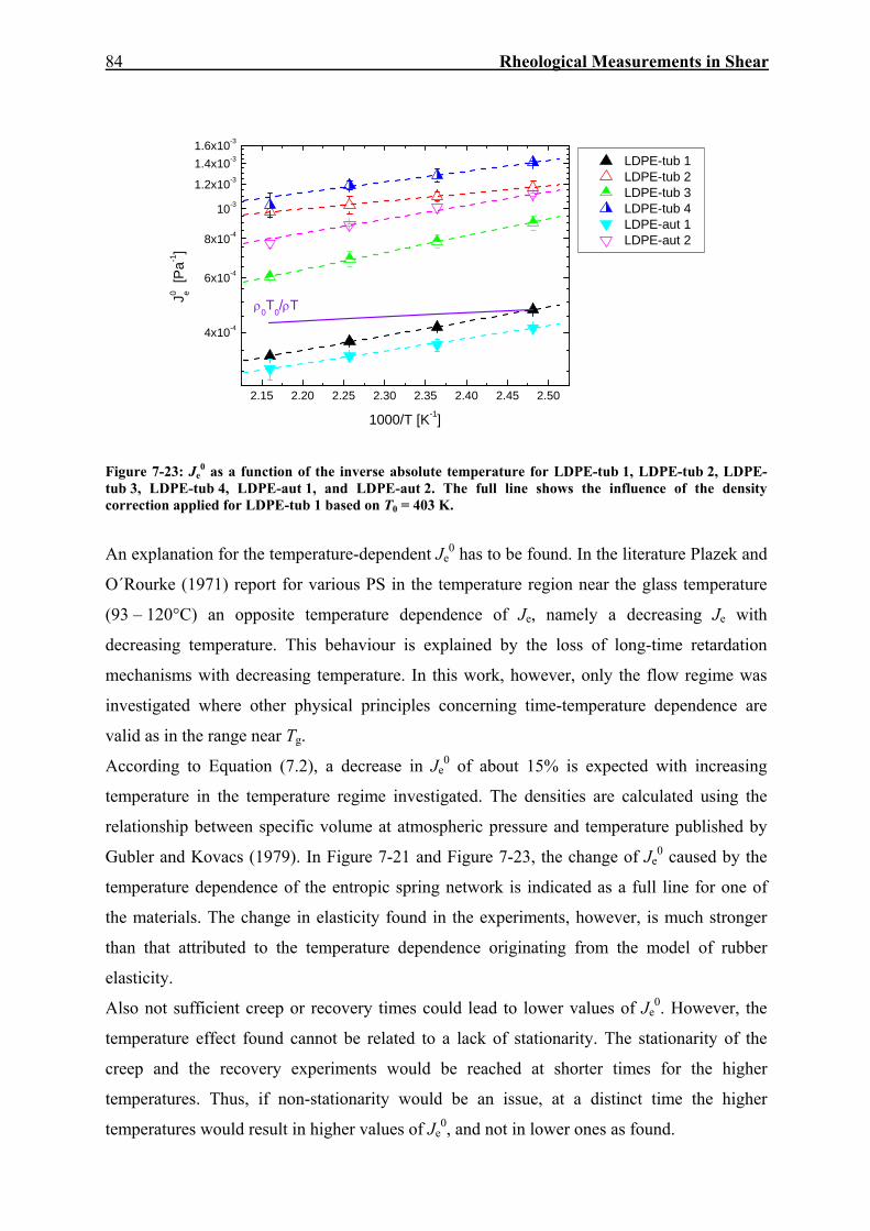
84 Rheological Measurements in Shear
2.15 2.20 2.25 2.30 2.35 2.40 2.45 2.50
4x10⁻⁴
6x10⁻⁴
8x10⁻⁴
10-3
1.2x10⁻³
1.4x10-31.6x10-3
ρ0T0/ρT
LDPE-tub 1 LDPE-tub 2 LDPE-tub 3 LDPE-tub 4 LDPE-aut 1 LDPE-aut 2
J0 e [P
a-1]
1000/T [K-1]
Figure 7-23: Je
0 as a function of the inverse absolute temperature for LDPE-tub 1, LDPE-tub 2, LDPE-tub 3, LDPE-tub 4, LDPE-aut 1, and LDPE-aut 2. The full line shows the influence of the density correction applied for LDPE-tub 1 based on T0 = 403 K.
An explanation for the temperature-dependent Je0 has to be found. In the literature Plazek and
O´Rourke (1971) report for various PS in the temperature region near the glass temperature
(93 – 120°C) an opposite temperature dependence of Je, namely a decreasing Je with
decreasing temperature. This behaviour is explained by the loss of long-time retardation
mechanisms with decreasing temperature. In this work, however, only the flow regime was
investigated where other physical principles concerning time-temperature dependence are
valid as in the range near Tg.
According to Equation (7.2), a decrease in Je0 of about 15% is expected with increasing
temperature in the temperature regime investigated. The densities are calculated using the
relationship between specific volume at atmospheric pressure and temperature published by
Gubler and Kovacs (1979). In Figure 7-21 and Figure 7-23, the change of Je0 caused by the
temperature dependence of the entropic spring network is indicated as a full line for one of
the materials. The change in elasticity found in the experiments, however, is much stronger
than that attributed to the temperature dependence originating from the model of rubber
elasticity.
Also not sufficient creep or recovery times could lead to lower values of Je0. However, the
temperature effect found cannot be related to a lack of stationarity. The stationarity of the
creep and the recovery experiments would be reached at shorter times for the higher
temperatures. Thus, if non-stationarity would be an issue, at a distinct time the higher
temperatures would result in higher values of Je0, and not in lower ones as found.

Rheological Measurements in Shear
85
As the model of rubber elasticity and possible experimental shortcomings do not explain the
temperature dependencies of Je0, the reason must be found in the molecular structure of the
LCB-mLLDPE and LDPE. As already pointed out earlier in this chapter and also confirmed
by SEC-MALLS measurements the LCB-mLLDPE have to be considered as blends of linear,
starlike branched molecules, and a few even more highly branched molecules, e.g., H-shaped
species. Consequently, this behaviour similar to a blend should also be visible in the
retardation and relaxation spectra by the presence of different relaxation modes that can be
correlated to the different molecular species.
According to the literature for the LCB-mLLDPE, two main retardation or relaxation regimes
have to be assumed (Wood-Adams, 2001, Malmberg et al., 2002, Gabriel et al., 2002, Stadler
et al., 2006a). That one at shorter times is interpreted to correspond to the linear chains with
low molar masses, while the longer one is assumed to be the consequence of the long-chain
branched chains of higher relaxation or retardation times, respectively. In this interpretation,
the linear molecules dominate the short retardation times and the branched molecules the
longer ones. As an example, these assumptions are visualized in Figure 7-24 in which for two
different temperatures the retardation spectra of the components as well as of the blend are
shown. For the reason of simplicity, the same shape of the spectra is assumed for the linear
and the LCB component. The spectrum of the blend was obtained by a linear superposition,
which excludes any interaction between the two blend components.
From the retardation spectrum L(τ ) Je0 can directly be calculated as it is simply the integral
over the whole spectrum:
∫∞
∞−
= ττ log)(0 dLJe (7.3)
As long-chain branched polyethylenes have a much higher activation energy than linear ones
(cf. Table 7-1), a change of the temperature influences the mobility of the linear and branched
molecules differently. Due to the higher activation energy of the long-chain branched
molecules, their retardation times are increased more by a decrease in temperature than those
of the linear species (see Figure 7-24). Therefore, the assumed difference in retardation times
between the linear and the long-chain branched molecules will increase. As a consequence,
Je0 will become temperature-dependent.

86 Rheological Measurements in Shear
log aT1(linear)
T1
LCB blend
log τ
log
L
linear
T2
log aT2(LCB)
T1 > T2
Figure 7-24: Schematic picture of the temperature dependence of the retardation spectrum L(τ ) of a blend of linear and LCB molecules with different temperature dependencies (Resch et al., 2009).
Since the activation energy of the LCB molecules is larger than that of the linear ones a
decrease in temperature makes the spread of the retardation spectrum on the retardation time
axis broader (Figure 7-24). Consequently, the integral according to Equation (7.3), and
therefore, Je0 becomes larger.
The findings of the temperature dependence of the LDPE samples can also be explained by
the previous assumptions. In LDPE all molecules are long-chain branched. From the SEC-
MALLS data (Figure 6-6 and Figure 6-7) it can be concluded that the braching topography
changes with molar mass. It is not too hypothetical to assume, however, that the differences
in activation energies will be smaller compared to those between linear and LCB molecules.
As a consequence, the temperature dependence of Je0 will become less pronounced.
Examples for discrete retardation spectra ji(τ ) determined from measurements at 130 and
190°C are given in Figure 7-25 (a) and Figure 7-25 (b) for LCB-mLLDPE 3 and LDPE-tub 4,
respectively. They are determined from the discrete relaxation spectra by Schwarzl (2008)
according to the method of Baumgärtel and Winter (1989). From the discrete retardation
spectrum Je0 is calculated with ji being the retardation strength as follows:
∑=
=n
iie jJ
1
0 (7.4)

Rheological Measurements in Shear
87
10-4 10-3 10-2 10-1 100 101 102 103 10410-7
10-6
10-5
10-4j i [P
a-1]
τi [s]
130°C 190°C
LCB-mLLDPE 3
(a)10-4 10-3 10-2 10-1 100 101 102 103 104 105
10-6
10-5
10-4
10-3
j i [Pa-1
]
τi [s]
130°C 190°C
LDPE-tub 4
(b)
Figure 7-25: Temperature dependence of retardation spectra ji( iτ ) for (a) LCB-mLLDPE 3 and (b) LDPE-tub 4.
Compared to the schematic continuous retardation spectrum L(τ ) from Figure 7-24 the shape
of ji( iτ ) differs. The two main relaxation modes postulated for LCB-mLLDPE cannot be
distinguished for LCB-mLLDPE 3 from Figure 7-25 (a), presumably because the two
relaxation modes do not differ strongly enough in retardation time and the spectra are
additionally smoothed by the molar mass distribution being 2.4.
As from the retardation spectra the retardation processes corresponding to the different
molecular species cannot be clearly resolved, the relaxation spectra are also discussed in the
following. A schematic picture of the temperature dependence of the relaxation spectrum
H(τ) of a blend of linear and LCB molecules having different activation energies is presented
in Figure 7-26. In agreement with the literature, two main relaxation regimes are assumed for
the LCB-mLLDPE (Wood-Adams, 2001, Malmberg et al., 2002, Gabriel et al., 2002, Stadler
et al., 2006a). The dotted lines in Figure 7-26 indicate the shape of the spectrum for a
polymer containing only linear molecules. With decreasing temperature, the whole spectrum
shifts towards longer relaxation times. The activation energy of the LCB molecules is higher
than that of the linear molecules, and therefore, the shift factor aT that shifts the spectrum
must be higher for the LCB component, too. The parts of the spectrum at the short relaxation
times shift with a smaller shift factor aT1 corresponding to the linear molecules. The parts of
the spectrum at the long relaxation times corresponding to the LCB molecules shift with a
larger shift factor aT2. The different shift factors are indicated in the picture by arrows of
different lengths. Thus, the spectra are temperature-dependent leading to a
thermorheologically complex behaviour of the polymer.

88 Rheological Measurements in Shear
log aT2
regime of longrelaxation times:LCB molecules
T1
T2
linear molecules T1
linear molecules T2
log
H [P
a]
τ [s]
T1>T2
regime of shortrelaxation times:linear molecules
log aT1
Figure 7-26: Schematic picture of the temperature dependence of the relaxation spectrum H(τ) for a blend of linear and LCB molecules with different temperature dependencies.
For the LCB-mLLDPE 3 the relaxation spectra H(τ) calculated for four different temperatures
130, 150, 170, and 190°C are plotted in Figure 7-27. The spectra presented in this chapter for
LCB-mLLDPE 3, LDPE 4, mLLDPE 4, and PP 10 are calculated by Stadler (2009) according
to the method of Stadler and Bailly (2009) from frequency sweeps extended by creep-
recovery data. An overview of spectra calculation is given in Appendix 12.5.
The shapes of the relaxation spectra of LCB-mLLDPE 3 are as expected from the model,
however, the sharp transition zone between linear and LCB molecules as shown in the
schematic drawing is smoother due to effects of the molar mass distribution. This result is
quite surprising as in the retardation spectrum of LCB-mLLDPE 3 no clear evidence for two
different retardation modes is found. With a shift factor aT1 = 4 determined in the short
relaxation time regime it is not possible to shift the whole curve for 190°C onto the curve for
130°C. The shift factor aT1 = 4 corresponds to an Ea of 35.8 kJ mol-1 a value in accordance to
the values given in Table 7-1 for the linear mLLDPE. For the long relaxation time regime a
larger shift factor aT2 = 8 that corresponds to an Ea of 53.8 kJ mol-1 has to be applied. The
LCB component with the high activation energy and the large shift factor mainly contributes
to the long relaxation times, whereas, the linear component with the low activation energy
and the small shift factor contributes to the short relaxation times. Thus, the assumption of a
behaviour like a blend for the LCB-mLLDPE seems to be confirmed by the analysis of the
relaxation spectra. The activation energie of 48.9 kJ mol-1 determined from the zero shear-rate
viscosities for LCB-mLLDPE 3 (see Table 7-1) lies inbetween the values corresponding to

Rheological Measurements in Shear
89
the linear and the long-chain branched component and represents, thus, a value comprising
the contributions of the linear as well as the long-chain branched species.
10-3 10-2 10-1 100 101 102 103100
101
102
103
104
105
106
log aT2= log aT1+ c 130 150 170 190 190 shifted with aT1= 4
H [P
a]
τ [s]
LCB-mLLDPE 3
log aT1
T [°C]
Figure 7-27: Relaxation spectra H(τ) of LCB-mLLDPE 3 determined at four different temperatures 130, 150, 170, and 190°C.
The findings of the temperature dependence of Je0 of the LDPE samples can be explained by
the analysis of the relaxation spectra presented in Figure 7-28 using LDPE-tub 4 as an
example. For the LDPE no processes corresponding to specific molecular species can be
discriminated as in the case of the LCB-mLLDPE because the spectra are even smoother due
to the broad molar mass distribution. However, the non-uniform branching topography is also
reflected in the spectra of LDPE. In order to shift the spectrum at 190°C on top of the spectra
at 130°C at short relaxation times a smaller shift factor aT1 = 6 has to be applied compared to
the region of long relaxation times where a larger shift factor aT2 = 16 is valid. These shift
factors correspond to Ea of 46.4 kJ mol-1 and 71.7 kJ mol-1, respectively. However, in the case
of the LDPE the different relaxation processes cannot be attributed to specific molecular
topographies as changes in the branching structure occur continuously with molar mass. In
addition, the broad polydispersity of LDPE affects the shape of the spectrum. Therefore, the
change of the shift factors with increasing relaxation time occurs continuously along the
spectrum, too. The activation energy determined from the zero shear-rate viscosities of
68.5 kJ mol-1 (see Table 7-1) lies inbetween the values calculated from aT1 and aT2. Therefore,
it can be regarded as an average value taking into account the contributions of all molecular
species present.

90 Rheological Measurements in Shear
10-2 10-1 100 101 102 103 104 10510-1
100
101
102
103
104
105
log aT2= log aT1+ c
log aT1
H [P
a]
τ [s]
130 150 170 190 190 shifted with aT1= 6
LDPE-tub 4
T [°C]
Figure 7-28: Relaxation spectra H(τ) of LDPE-tub 4 determined at four different temperatures 130, 150, 170, and 190°C.
These considerations on the relaxation spectra also allow the interpretation of the missing
temperature dependence of Je0 of the linear PP. They consist only of linear molecules, which
means that all molecules have the same temperature dependence. In such a case, a change in
temperature leads to a shift of the whole spectrum by the same shift factor, leaving the shape
of the spectrum and the integral of Equation (7.3) unchanged. Figure 7-29 shows H(τ) of
PP 10 at 180, 200, and 220°C. Applying one shift factor aT1 = 2.5 corresponding to an Ea of
42.6 kJ mol-1 the spectrum at 220°C can be shifted on top of the spectrum at 180°C along the
whole range of relaxation times. In Table 7-1, a value for Ea of 40.9 kJ mol-1 calculated from
the zero shear-rate viscosities is listed for PP 10, that corresponds quite well to the one
determined from the relaxation spectra.
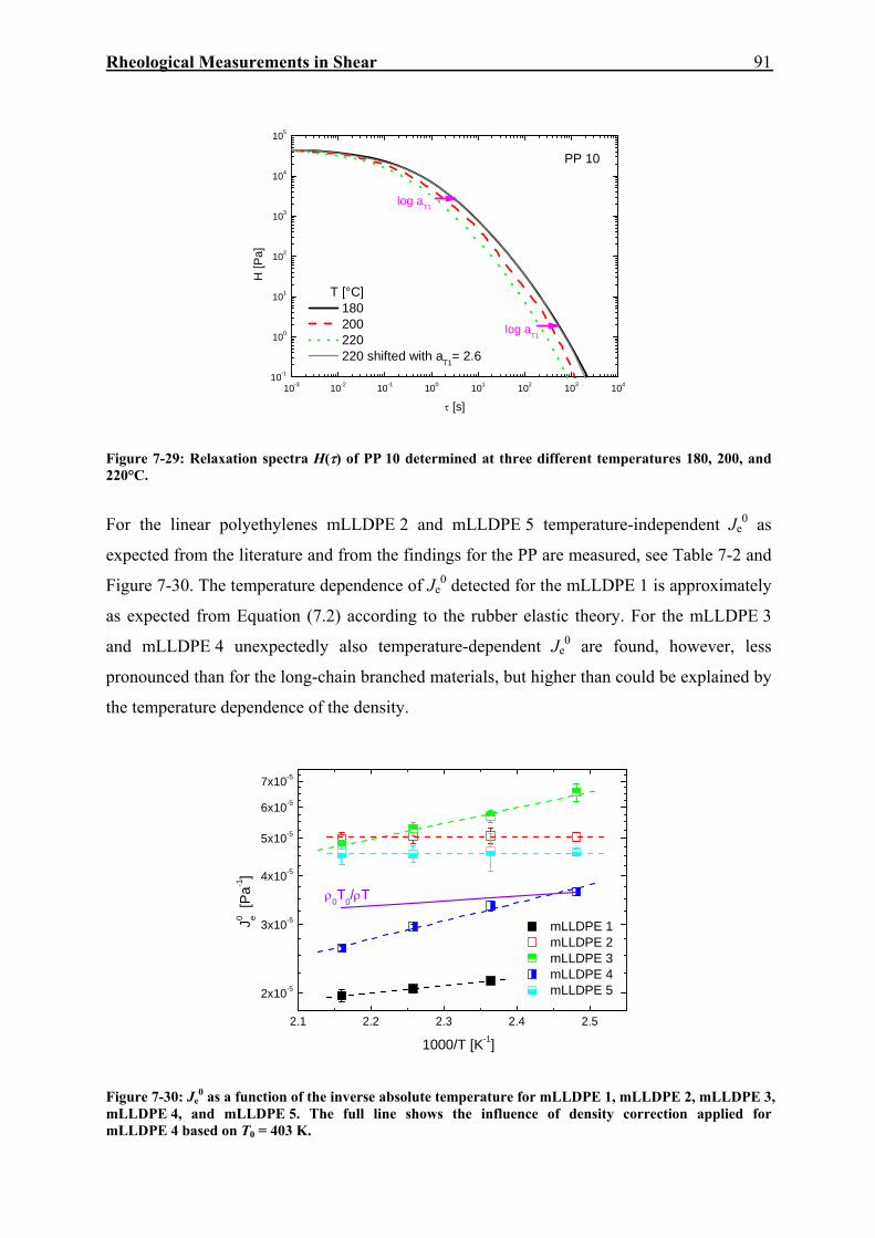
Rheological Measurements in Shear
91
10-3 10-2 10-1 100 101 102 103 10410-1
100
101
102
103
104
105
PP 10
log aT1
log aT1
T [°C]
H [P
a]
τ [s]
180 200 220 220 shifted with aT1= 2.6
Figure 7-29: Relaxation spectra H(τ) of PP 10 determined at three different temperatures 180, 200, and 220°C.
For the linear polyethylenes mLLDPE 2 and mLLDPE 5 temperature-independent Je0 as
expected from the literature and from the findings for the PP are measured, see Table 7-2 and
Figure 7-30. The temperature dependence of Je0 detected for the mLLDPE 1 is approximately
as expected from Equation (7.2) according to the rubber elastic theory. For the mLLDPE 3
and mLLDPE 4 unexpectedly also temperature-dependent Je0 are found, however, less
pronounced than for the long-chain branched materials, but higher than could be explained by
the temperature dependence of the density.
2.1 2.2 2.3 2.4 2.5
2x10⁻⁵
3x10⁻⁵
4x10⁻⁵
5x10⁻⁵
6x10⁻⁵
7x10⁻⁵
mLLDPE 1 mLLDPE 2 mLLDPE 3 mLLDPE 4 mLLDPE 5
ρ0T0/ρT
J0 e [P
a-1]
1000/T [K-1]
Figure 7-30: Je
0 as a function of the inverse absolute temperature for mLLDPE 1, mLLDPE 2, mLLDPE 3, mLLDPE 4, and mLLDPE 5. The full line shows the influence of density correction applied for mLLDPE 4 based on T0 = 403 K.
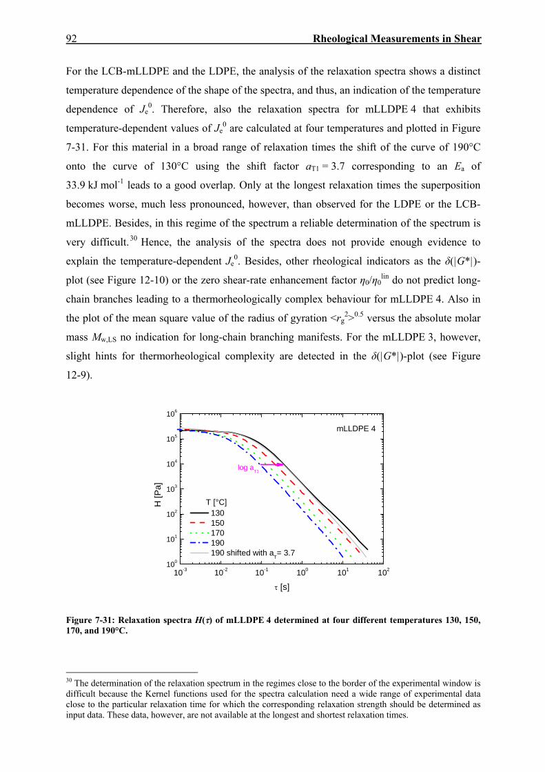
92 Rheological Measurements in Shear
For the LCB-mLLDPE and the LDPE, the analysis of the relaxation spectra shows a distinct
temperature dependence of the shape of the spectra, and thus, an indication of the temperature
dependence of Je0. Therefore, also the relaxation spectra for mLLDPE 4 that exhibits
temperature-dependent values of Je0 are calculated at four temperatures and plotted in Figure
7-31. For this material in a broad range of relaxation times the shift of the curve of 190°C
onto the curve of 130°C using the shift factor aT1 = 3.7 corresponding to an Ea of
33.9 kJ mol-1 leads to a good overlap. Only at the longest relaxation times the superposition
becomes worse, much less pronounced, however, than observed for the LDPE or the LCB-
mLLDPE. Besides, in this regime of the spectrum a reliable determination of the spectrum is
very difficult.30 Hence, the analysis of the spectra does not provide enough evidence to
explain the temperature-dependent Je0. Besides, other rheological indicators as the δ(|G*|)-
plot (see Figure 12-10) or the zero shear-rate enhancement factor η0/η0lin do not predict long-
chain branches leading to a thermorheologically complex behaviour for mLLDPE 4. Also in
the plot of the mean square value of the radius of gyration <rg2>0.5 versus the absolute molar
mass Mw,LS no indication for long-chain branching manifests. For the mLLDPE 3, however,
slight hints for thermorheological complexity are detected in the δ(|G*|)-plot (see Figure
12-9).
10-3 10-2 10-1 100 101 102100
101
102
103
104
105
106
log aT1
H [P
a]
τ [s]
130 150 170 190 190 shifted with aT= 3.7
mLLDPE 4
T [°C]
Figure 7-31: Relaxation spectra H(τ) of mLLDPE 4 determined at four different temperatures 130, 150, 170, and 190°C.
30 The determination of the relaxation spectrum in the regimes close to the border of the experimental window is difficult because the Kernel functions used for the spectra calculation need a wide range of experimental data close to the particular relaxation time for which the corresponding relaxation strength should be determined as input data. These data, however, are not available at the longest and shortest relaxation times.

Rheological Measurements in Shear
93
As from the analysis of the spectra no profound explanation for the temperature-dependent Je0
was found, other reasons have to be considered. An explanation might be possible regarding
the significantly higher comonomer content of mLLDPE 3 and mLLDPE 4 compared to
mLLDPE 1, mLLDPE 2, and mLLDPE 5, as can be seen from the melting temperatures Tm
(see Table 6-1) and the melting peaks in Figure 6-9. It is known from the literature that the
comonomer does not influence η0 (Stadler, 2007). Also the plot of <rg2>0.5 versus Mw,LS is
only marginally affected by the comonomer.31 All materials plotted in Figure 6-9 show broad
melting peaks and a shoulder or even a second peak indicating different crystalline structures,
and thus, an inhomogeneous comonomer insertion. It is assumed that in the case of
mLLDPE 3 and mLLDPE 4 these different species give a hint to different activation energies
in the molten state. In comparison mLLDPE 1, mLLDPE 2, and mLLDPE 5 contain little
comonomer and the molecular species present in these materials can be assumed to have
similar activation energies. Vega et al. (1998, 1999) and Stadler (2007) report an increase in
Ea with increasing comonomer content. As mentioned before, if a material contains molecules
with different molecular structures whose activation energies differ, this difference in
activation energies leads to a temperature-dependent shape of the spectra and a
thermorheological complexity. In the case of mLLDPE 3 and mLLDPE 4, these different
molecular structures could be caused by an inhomogeneous comonomer distribution. It can be
assumed that the comonomer is not equally distributed among the short and the long
molecules. From the analysis of the relaxation of spectra of mLLDPE 4, it seems that the long
molecules contributing to the long relaxation times contain more comonomer as in this
regime of the spectra a larger shift factor has to be applied to overlap the spectra.
31 With increasing comonomer content the linear correlation in the double-logarithmic plot between <rg
2>0.5 and Mw,LS shifts to downwards. The slope of the line, however, remains unaffected.
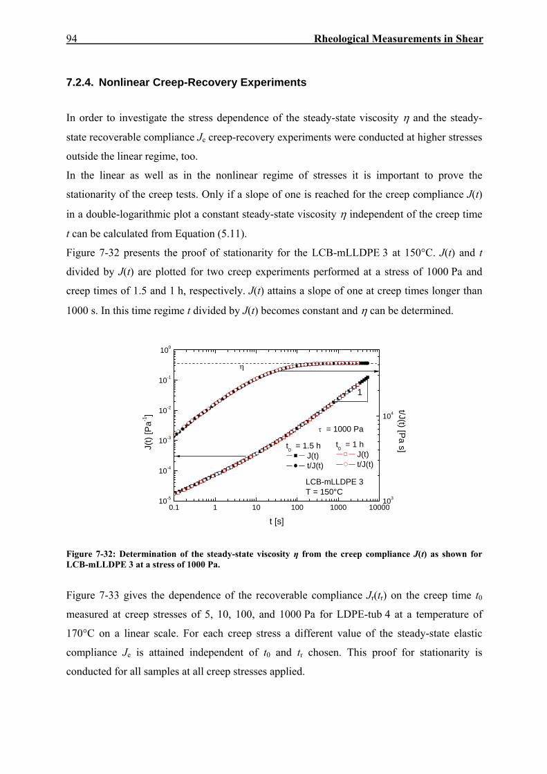
94 Rheological Measurements in Shear
7.2.4. Nonlinear Creep-Recovery Experiments
In order to investigate the stress dependence of the steady-state viscosity η and the steady-
state recoverable compliance Je creep-recovery experiments were conducted at higher stresses
outside the linear regime, too.
In the linear as well as in the nonlinear regime of stresses it is important to prove the
stationarity of the creep tests. Only if a slope of one is reached for the creep compliance J(t)
in a double-logarithmic plot a constant steady-state viscosity η independent of the creep time
t can be calculated from Equation (5.11).
Figure 7-32 presents the proof of stationarity for the LCB-mLLDPE 3 at 150°C. J(t) and t
divided by J(t) are plotted for two creep experiments performed at a stress of 1000 Pa and
creep times of 1.5 and 1 h, respectively. J(t) attains a slope of one at creep times longer than
1000 s. In this time regime t divided by J(t) becomes constant and η can be determined.
0.1 1 10 100 1000 1000010-5
10-4
10-3
10-2
10-1
100
t0 = 1 ht0 = 1.5 h J(t) t/J(t)
J(t) t/J(t)
t [s]
J(t)
[Pa-1
]
1
LCB-mLLDPE 3T = 150°C
τ = 1000 Pa
η
103
104
t/J(t) [Pa s]
Figure 7-32: Determination of the steady-state viscosity η from the creep compliance J(t) as shown for LCB-mLLDPE 3 at a stress of 1000 Pa.
Figure 7-33 gives the dependence of the recoverable compliance Jr(tr) on the creep time t0
measured at creep stresses of 5, 10, 100, and 1000 Pa for LDPE-tub 4 at a temperature of
170°C on a linear scale. For each creep stress a different value of the steady-state elastic
compliance Je is attained independent of t0 and tr chosen. This proof for stationarity is
conducted for all samples at all creep stresses applied.

Rheological Measurements in Shear
95
0 10000 20000 30000 400000.0
2.0x10⁻⁴
4.0x10⁻⁴
6.0x10⁻⁴
8.0x10⁻⁴
1.0x10⁻³
1.2x10⁻³
1.4x10⁻³
t0 = 5 h t0 = 4 h t0 = 3 h
t0 = 5 h t0 = 4 h
τ = 10 Pa τ = 100 Pa τ = 1000 Pa t0 = 5 h
τ = 5 Pa t0 = 4 h
J r(tr)
[Pa-1
]
tr [s]
LDPE-tub 4T = 170°C
Figure 7-33: Jr(tr) for LDPE-tub 4 at 170°C measured at various shear stresses and different times of the preceding creep test t0.
Figure 7-33 also shows that measurements at τ = 5 Pa and τ = 10 Pa give the linear steady-
state elastic compliance Je0, whereas, with increasing creep stress Je decreases.
The stress dependencies of J(t) and Jr(tr) for all stresses measured are shown exemplarily for
PP 10 at 180°C in Figure 7-34 and for mLLDPE 4 at 170°C in Figure 7-35.32 For both
materials with distinctly different Je0 the decrease in Je with increasing stress is obvious. At
short t and tr the curves of J(t) and Jr(tr) fall on top of each other independent of the creep
stress τ. The higher τ the stronger is the deviation from the linear Jr(tr) curve and the sooner Je
is attained.
Concerning J(t) in the case of PP 10, the deviation at higher stresses from the linear J(t) is not
as pronounced as the effect on Jr(tr). For mLLDPE 4 even all curves of J(t) coincide, whereas,
the Jr(tr) curves show a significant stress dependence. This coincidence of J(t) for all creep
stresses τ implies that the viscosities are the same independent of τ, and thus, no shear
thinning is present. For PP 10, however, the stress-dependent J(t) also involve stress-
dependent η as η can be calculated from J(t) by Equation (5.11).
32 For most of the other materials the stress dependence of J(t) and Jr(tr) was measured, too, sometimes even at various temperatures. Their presentation, however, goes beyond the scope of this work.

96 Rheological Measurements in Shear
0.1 1 10 100 1000 1000010-5
10-4
10-3
10-2
10-1
τ = 200 Pa τ = 400 Pa τ = 600 Pa τ = 1000 Pa τ = 3000 Pa τ = 5000 Pa
τ = 2 Pa τ = 5 Pa τ = 10 Pa τ = 15 Pa τ = 20 Pa τ = 50 Pa τ = 100 Pa
J(t),
Jr(t 0,t r) [
Pa-1]
t, tr [s]
PP 10T = 180°C
Figure 7-34: J(t) and Jr(tr) at various shear stresses for PP 10 at 180°C (Wolff et al., 2010).
0.1 1 10 10010-6
10-5
10-4
10-3
10-2
τ = 300 Pa τ = 1000 Pa τ = 2000 Pa τ = 3000 Pa τ = 5000 Pa τ = 10 000 Pa
τ = 5 Pa τ = 10 Pa τ = 20 Pa τ = 30 Pa τ = 50 Pa τ = 100 Pa
J(t),
Jr(t 0,t r) [
Pa-1]
t, tr [s]
mLLDPE 4T = 170°C
Figure 7-35: J(t) and Jr(tr) at various shear stresses for mLLDPE 4 at 170°C.
The stress dependence of η and Je can be visualized best when plotting only the stationary
values of η and Je as a function of creep stress τ. This is shown for PP 10 at three measuring
temperatures for η in Figure 7-36 and for Je in Figure 7-37.33
33 The η and Je presented in Figure 7-36 and Figure 7-37 are average values of at least three measurements. At the highest measuring temperature of 220°C, only Je
0 was determined.

Rheological Measurements in Shear
97
1 10 100 1000 10000
2x10⁴
3x10⁴
4x10⁴
5x10⁴
6x10⁴
7x10⁴
8x10⁴
PP 10 180 200 220
η [P
a s]
τ [Pa]
T [°C]
Figure 7-36: Stress dependence of the steady-state viscosity η for PP 10 at 180, 200, and 220°C (Wolff, 2008).
1 10 100 1000 1000010-4
10-3
J e [Pa-1
]
τ [Pa]
180 200 220
PP 10 T [°C]
Figure 7-37: Stress dependence of the steady-state elastic compliance Je for PP 10 at 180, 200, and 220°C (Wolff, 2008).
Figure 7-36 and Figure 7-37 confirm that the onset of the nonlinear regime occurs at much
lower stresses for Je than for η. This result is observed for all materials investigated and will
be discussed in Chapter 7.2.5.
Furthermore, it can be seen that in the nonlinear regime of stresses Je is temperature-
independent.
Figure 7-38 presents Jr(tr) of PP 10 measured at 1000 Pa at three different measuring
temperatures. As in the linear stress regime (see Figure 7-18) the Jr(tr) curves for the different
measuring temperatures do not merge. The higher the measuring temperature the higher lies

98 Rheological Measurements in Shear
the Jr(tr) curve corresponding to a time-temperature shift. At long measuring times, however,
the Jr(tr) curves measured at different temperatures all yield the same value for Je. The
construction of a mastercurve is shown in Appendix 12.4 in Figure 12-12.
0.1 1 10 100 1000 1000010-5
10-4
10-3
180 200 220
J r(tr)
[Pa-1
]
tr [s]
PP 10
T [°C] τ = 1000 Pa
Figure 7-38: Recoverable compliance Jr(tr) as a function of recovery time for the linear polypropylene PP 10 at measuring temperatures of 180, 200, and 220°C for a creep stress τ of 1000 Pa (Wolff, 2008).
In Figure 7-39, Jr(tr) and J(t) for the LCB-mLLDPE 3 are plotted for the four measuring
temperatures 130, 150, 170, and 190°C. For the thermorheologically complex materials the
analysis of Jr(tr) in the linear stress regime (see Figure 7-20) and in the nonlinear stress
regime give the same result. At short times when the viscous contribution to J(t) is still
negligible Jr(tr) and J(t) are nearly identical. Then the curves of Jr(tr) for the different
temperature cross each other and reach different stationary values of Je. The failure of the
construction of a mastercurve is presented in Appendix 12.4 in Figure 12-14.

Rheological Measurements in Shear
99
1 10 100 1000 10000103
104
130°C 150°C 170°C 190°C mLLDPE 4
η [P
a s]
τ [Pa] (a)
0.1 1 10 100 1000 1000010-5
10-4
10-3
10-2
10-1
LCB-mLLDPE 3τ = 1000 Pa
J
J(t),
Jr(t
r) [P
a-1]
t, tr [s]
130°C 150°C 170°C 190°C
Jr T
Figure 7-39: Creep compliance J(t) and recoverable compliance Jr(tr) as a function of time for LCB-mLLPDE 3 at measuring temperatures of 130, 150, 170, and 190°C and a creep stress τ of 1000 Pa.
• Construction of mastercurves for η(τ)
In Figure 7-36, η as function of τ is presented for PP 10.34 The values for η and the error bars
in this figure and in the following figures presenting η as function of τ result from averaging
at least three individual measurements. The same plot (Figure 7-40 (a)) is also constructed for
the linear mLLDPE 4 at four measuring temperatures. As already assumed from Figure 7-35
mLLDPE 4 exhibits no or only very slight shear thinning.
Figure 7-40: (a) Stress dependence of the steady-state viscosity η for mLLDPE 4 at 130, 150, 170, and 190°C. (b) Mastercurve of the steady-state viscosity η as a function of stress τ for mLLDPE 4 at a reference temperature of T0 = 170°C.
34 The construction of a mastercurve for η as a function of τ for PP 10 at a reference temperature of 200°C is presented in Appendix 12.9 in Figure 12-22.
1 10 100 1000 10000
8x10³
9x10³
104
130°C 150°C 170°C 190°C averages
mLLDPE 4
η⋅a T [P
a s]
τ [Pa]
T0 = 170°C
(b)

100 Rheological Measurements in Shear
It is shown in Figure 7-40 (b) for mLLDPE 4 and a reference temperature T0 = 170°C that the
curves for η as a function of τ can be shifted on top of each other. The shift factors aT used
correspond to the shift factors calculated from the zero shear-rate viscosities according to
Equation (7.1). An average curve is calculated from the η(τ) at the different measuring
temperatures. The error bars at the respective stresses represent averages of the error bars at
the different temperatures.35
Despite thermorheological complexity the curves of η(τ) at the four measuring temperatures
for the thermorheologically complex materials can be shifted on top of each other
(T0 = 170°C). Figure 7-41 (a) and Figure 7-41 (b) and Figure 7-42 (a) and Figure 7-42 (b)
present for LCB-mLLDPE 3 and LDPE-tub 1, respectively, the curves for η(τ) at the different
measuring temperatures, the shifted curves, and the average curve calculated from the shifted
curves.
For all material classes (mLLDPE, LCB-mLLDPE, and LDPE) the curves can be shifted on
top of each other along the whole stress range with one shift factor aT, which corresponds to
the shift factor determined from η0. The finding of mastercurves for η(τ) even for
thermorheologically complex materials means that the steady-state viscous quantity η does
not reflect the thermorheologically complex behaviour.
For further materials η(τ) at different temperatures is determined, too. Their viscosity data
can be found in Appendix 12.9.
Figure 7-41: (a) Stress dependence of the steady-state viscosity η for LCB-mLLDPE 3 at 130, 150, 170, and 190°C. (b) Mastercurve of the steady-state viscosity η as a function of stress τ for LCB-mLLDPE 3 at a reference temperature of T0 = 170°C.
35 The calculation of η from J(t) for stresses in the nonlinear range bases on the assumption that J(t) can be separated into a viscous term, a viscoelastic part, and an instantaneous compliance as given by Equation (5.10).
1 10 100 1000 10000
104
1.5x10⁴
2x10⁴
130°C 150°C 170°C 190°C
η⋅a T [P
a s]
τ [Pa]
LCB-mLLDPE 3
averagesT0 = 170°C
(b)1 10 100 1000 10000
104
105
130°C 150°C 170°C 190°C
η [P
a s]
τ [Pa]
LCB-mLLDPE 3
(a)
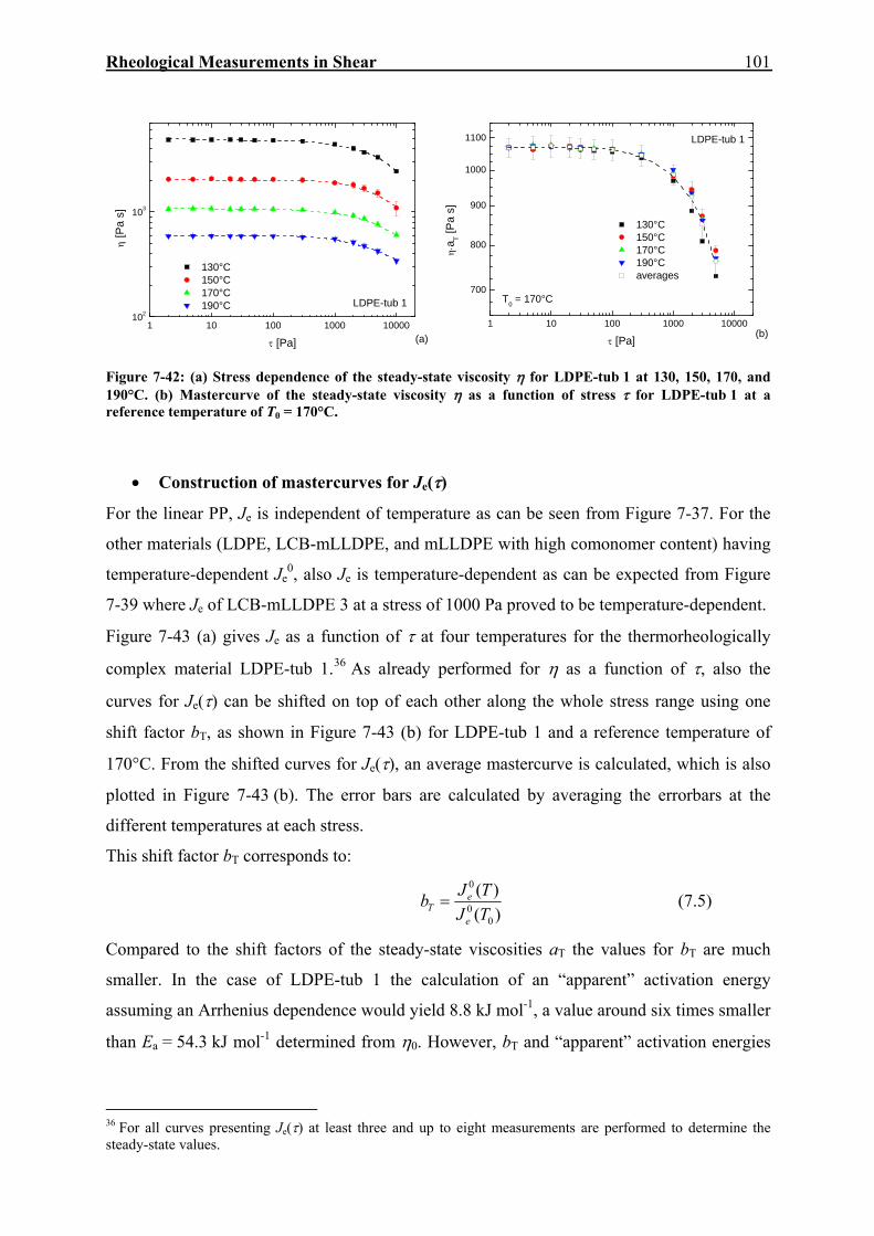
Rheological Measurements in Shear
101
Figure 7-42: (a) Stress dependence of the steady-state viscosity η for LDPE-tub 1 at 130, 150, 170, and 190°C. (b) Mastercurve of the steady-state viscosity η as a function of stress τ for LDPE-tub 1 at a reference temperature of T0 = 170°C.
• Construction of mastercurves for Je(τ)
For the linear PP, Je is independent of temperature as can be seen from Figure 7-37. For the
other materials (LDPE, LCB-mLLDPE, and mLLDPE with high comonomer content) having
temperature-dependent Je0, also Je is temperature-dependent as can be expected from Figure
7-39 where Je of LCB-mLLDPE 3 at a stress of 1000 Pa proved to be temperature-dependent.
Figure 7-43 (a) gives Je as a function of τ at four temperatures for the thermorheologically
complex material LDPE-tub 1.36 As already performed for η as a function of τ, also the
curves for Je(τ) can be shifted on top of each other along the whole stress range using one
shift factor bT, as shown in Figure 7-43 (b) for LDPE-tub 1 and a reference temperature of
170°C. From the shifted curves for Je(τ), an average mastercurve is calculated, which is also
plotted in Figure 7-43 (b). The error bars are calculated by averaging the errorbars at the
different temperatures at each stress.
This shift factor bT corresponds to:
)()(
00
0
TJTJb
e
eT = (7.5)
Compared to the shift factors of the steady-state viscosities aT the values for bT are much
smaller. In the case of LDPE-tub 1 the calculation of an “apparent” activation energy
assuming an Arrhenius dependence would yield 8.8 kJ mol-1, a value around six times smaller
than Ea = 54.3 kJ mol-1 determined from η0. However, bT and “apparent” activation energies
36 For all curves presenting Je(τ) at least three and up to eight measurements are performed to determine the steady-state values.
1 10 100 1000 10000
700
800
900
1000
1100
130°C 150°C 170°C 190°C averages
η⋅a T [P
a s]
τ [Pa]
LDPE-tub 1
T0 = 170°C
(b)1 10 100 1000 10000
102
103
130°C 150°C 170°C 190°C LDPE-tub 1
η [P
a s]
τ [Pa] (a)

102 Rheological Measurements in Shear
are not further discussed because the mechanisms causing the temperature dependence of Je
are not fully understood.37
Figure 7-43: (a) Stress dependence of the steady-state elastic compliance Je for LDPE-tub 1 at 130, 150, 170, and 190°C. (b) Mastercurve of the steady-state elastic compliance Je as a function of stress τ for LDPE-tub 1 at a reference temperature of T0 = 170°C.
Also for products of other material classes (LCB-mLLDPE and linear mLLDPE)
mastercurves of Je(τ) are constructed. The results are shown in Figure 7-44, Figure 7-45, and
Figure 7-46 that present Je(τ) at the four measuring temperatures, Je(τ) shifted to a reference
temperature of 170°C, and the mastercurves of Je(τ) for LCB-mLLDPE 3, mLLDPE 4, and
mLLDPE 1, respectively.
Concerning mLLDPE 1, in Chapter 7.2.3 it is pointed out that Je0 of this material containing
only little comonomer can be regarded as temperature-independent. However, Je0 of
mLLDPE 1 exhibits a slight temperature dependence in the order of magnitude expected from
the theory of rubber elasticity as indicated in Figure 7-30. When plotting Je as a function of τ
the error bars for this low elastic material overlap for all temperatures and stresses (see Figure
7-46).
For further materials Je(τ) is determined too, the elasticity data can be found in Appendix 12.9.
37 Keßner et al. (2009) report an Arrhenius dependence of bT and “apparent” shift factors.
1 10 100 1000 100001.0x10-4
2.0x10⁻⁴
3.0x10⁻⁴
4.0x10⁻⁴
5.0x10⁻⁴ LDPE-tub 1
J e [Pa-1
]
τ [Pa]
130°C 150°C 170°C 190°C
(a)
1 10 100 1000 10000
1.5x10⁻⁴
2x10⁻⁴
2.5x10⁻⁴
3x10⁻⁴
3.5x10⁻⁴
4x10⁻⁴
T0 = 170°C
130°C 150°C 170°C 190°C averages
J e⋅bT [P
a-1]
τ [Pa]
LDPE-tub 1
(b)

Rheological Measurements in Shear
103
Figure 7-44: (a) Stress dependence of the steady-state elastic compliance Je for LCB-mLLDPE 3 at 130, 150, 170, and 190°C. (b) Mastercurve of the steady-state elastic compliance Je as a function of stress τ for LCB-mLLDPE 3 at a reference temperature of T0 = 170°C.
Figure 7-45: (a) Stress dependence of the steady-state elastic compliance Je for mLLDPE 4 at 130, 150, 170, and 190°C. (b) Mastercurve of the steady-state elastic compliance Je as a function of stress τ for mLLDPE 4 at a reference temperature of T0 = 170°C.
1 10 100 1000 1000010-5
1.5x10⁻⁵
2x10⁻⁵
2.5x10⁻⁵
3x10⁻⁵
150°C 170°C 190°C
J e [Pa-1
]
τ [Pa]
mLLDPE 1
Figure 7-46: Stress dependence of the steady-state elastic compliance Je for mLLDPE 1 at 150, 170, and 190°C.
1 10 100 1000 10000
10-4
2x10⁻⁴
3x10⁻⁴
4x10⁻⁴ LCB-mLLDPE 3
J e⋅bT [
Pa-1]
τ [Pa]
130°C 150°C 170°C 190°C averages
T0 = 170°C
(b)1 10 100 1000 10000
10-4
2x10⁻⁴
3x10⁻⁴
4x10⁻⁴
5x10⁻⁴
6x10⁻⁴
130°C 150°C 170°C 190°C
LCB-mLLDPE 3
J e [P
a-1]
τ [Pa] (a)
1 10 100 1000 1000010-5
2x10⁻⁵
3x10⁻⁵
4x10⁻⁵
5x10⁻⁵
6x10⁻⁵
130°C 150°C 170°C 190°C
mLLDPE 4
J e [Pa-1
]
τ [Pa] (a)1 10 100 1000 10000
10-5
2x10⁻⁵
3x10⁻⁵
4x10⁻⁵
130°C 150°C 170°C 190°C averages
mLLDPE 4
J e⋅b
T [Pa-1
]
τ [Pa]
T0 = 170°C
(b)
104 Rheological Measurements in Shear
Concerning the temperature dependence of Je in the nonlinear regime of stresses, Plazek and
O´Rourke (1971) find for linear PS that Je (measured at temperatures well above Tg) is the
same at different temperatures when the stresses are the same. The measurments on the linear
PP 10 (see Figure 7-37) give the same result. As temperature-dependent Je0 and Je for
thermorheologically complex materials are not reported in the literature, also the result that
the shift factor determined in the linear regime from Je0 can be applied to Je as function of
stress to construct a master curve is new. A discussion on this topic will be given in Chapter
7.2.6.
7.2.5. Correlation of Stress Dependence of Viscosity and Elasticity with Molecular Structure
• Polyethylenes
The stress dependence of the steady-state elastic compliance Je and the steady-state viscosity
η is determined as presented in the previous Chapter 7.2.4. In the following diagrammes for
the polyethylenes mLLDPE 1, mLLDPE 4, mLLDPE 5, LCB-mLLDPE 2, LCB-mLLDPE 3,
and LDPE-tub 1 the mastercurves at a reference temperature of 170°C are presented. For all
the other PE curves obtained at a single temperature of 170°C are discussed. The viscosities
and elasticities of the investigated materials differ by orders of magnitude, therefore, the
curves of Je(τ) and η(τ) are normalized by Je0 and η0 to make the comparison of the stress-
dependent behaviour easier. Figure 7-47 (a) presents the normalized viscosity η/η0 for the materials mLLDPE 1,
mLLDPE 4, and mLLDPE 5. The error bars in the following diagrammes are calculated by
propagation of uncertainty for η and η0 and Je and Je0, respectively. Concerning the viscosity,
all materials exhibit the same very weak shear thinning. At the highest stress measured
(10 000 Pa), η is 5% lower than η0 which is in the order of the measurement error. For linear
polymers only the polydispersity influences the shear-thinning behaviour, therefore, for these
materials having similar Mw/Mn between 2.2 and 2.9 the result presented was expected.
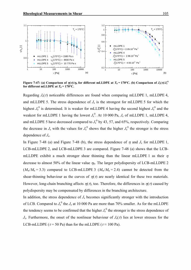
Rheological Measurements in Shear
105
Figure 7-47: (a) Comparison of η(τ)/η0 for different mLLDPE at T0 = 170°C. (b) Comparison of Je(τ)/Je
0 for different mLLDPE at T0 = 170°C. Regarding Je(τ) noticeable differences are found when comparing mLLDPE 1, mLLDPE 4,
and mLLDPE 5. The stress dependence of Je is the strongest for mLLDPE 5 for which the
highest Je0 is determined. It is weaker for mLLDPE 4 having the second highest Je
0 and the
weakest for mLLDPE 1 having the lowest Je0. At 10 000 Pa, Je of mLLDPE 1, mLLDPE 4,
and mLLDPE 5 have decreased compared to Je0 by 43, 57, and 65%, respectively. Comparing
the decrease in Je with the values for Je0 shows that the higher Je
0 the stronger is the stress
dependence of Je.
In Figure 7-48 (a) and Figure 7-48 (b), the stress dependence of η and Je for mLLDPE 1,
LCB-mLLDPE 2, and LCB-mLLDPE 3 are compared. Figure 7-48 (a) shows that the LCB-
mLLDPE exhibit a much stronger shear thinning than the linear mLLDPE 1 as their η
decrease to almost 50% of the linear value η0. The larger polydispersity of LCB-mLLDPE 2
(Mw/Mn = 3.3) compared to LCB-mLLDPE 3 (Mw/Mn = 2.4) cannot be detected from the
shear-thinning behaviour as the curves of η(τ) are nearly identical for these two materials.
However, long-chain branching affects η(τ), too. Therefore, the differences in η(τ) caused by
polydispersity may be compensated by differences in the branching architecture.
In addition, the stress dependence of Je becomes significantly stronger with the introduction
of LCB. Compared to Je0 the Je at 10 000 Pa are more than 70% smaller. As for the mLLDPE
the tendency seems to be confirmed that the higher Je0 the stronger is the stress dependence of
Je. Furthermore, the onset of the nonlinear behaviour of Je(τ) lies at lower stresses for the
LCB-mLLDPE (τ = 50 Pa) than for the mLLDPE (τ ≈ 100 Pa).
1 10 100 1000 10000
0.9
1
1.1
mLLDPE 1 η0(170°C) = 1580 Pa s mLLDPE 4 η0(170°C) = 8930 Pa s mLLDPE 5 η0(170°C) = 10 770 Pa s
η/η 0 [-
]
τ [Pa]
T0 = 170°C
(a)1 10 100 1000 10000
0.2
0.4
0.6
0.8
1
1.2
mLLDPE 1 J0
e(170°C) = 2.05⋅10-5 Pa-1 mLLDPE 4
J0e(170°C) = 2.96⋅10-5 Pa-1
mLLDPE 5 J0
e(170°C) = 4.55⋅10-5 Pa-1
J e/J0 e [-
]
τ [Pa]
T0 = 170°C
(b)
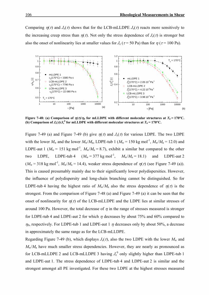
106 Rheological Measurements in Shear
Comparing η(τ) and Je(τ) shows that for the LCB-mLLDPE Je(τ) reacts more sensitively to
the increasing creep stress than η(τ). Not only the stress dependence of Je(τ) is stronger but
also the onset of nonlinearity lies at smaller values for Je (τ = 50 Pa) than for η (τ = 100 Pa).
Figure 7-48: (a) Comparison of η(τ)/η0 for mLLDPE with different molecular structures at T0 = 170°C. (b) Comparison of Je(τ)/Je
0 for mLLDPE with different molecular structures at T0 = 170°C.
Figure 7-49 (a) and Figure 7-49 (b) give η(τ) and Je(τ) for various LDPE. The two LDPE
with the lower Mw and the lower Mw/Mn, LDPE-tub 1 (Mw = 150 kg mol-1, Mw/Mn = 12.0) and
LDPE-aut 1 (Mw = 151 kg mol-1, Mw/Mn = 8.7), exhibit a similar but compared to the other
two LDPE, LDPE-tub 4 (Mw = 377 kg mol-1, Mw/Mn = 18.1) and LDPE-aut 2
(Mw = 318 kg mol-1, Mw/Mn = 14.4), weaker stress dependence of η(τ) (see Figure 7-49 (a)).
This is caused presumably mainly due to their significantly lower polydispersities. However,
the influence of polydispersity and long-chain branching cannot be distinguished. So for
LDPE-tub 4 having the highest ratio of Mw/Mn also the stress dependence of η(τ) is the
strongest. From the comparison of Figure 7-48 (a) and Figure 7-49 (a) it can be seen that the
onset of nonlinearity for η(τ) of the LCB-mLLDPE and the LDPE lies at similar stresses of
around 100 Pa. However, the total decrease of η in the range of stresses measured is stronger
for LDPE-tub 4 and LDPE-aut 2 for which η decreases by about 75% and 60% compared to
η0, respectively. For LDPE-tub 1 and LDPE-aut 1 η decreases only by about 50%, a decrease
in approximately the same range as for the LCB-mLLDPE.
Regarding Figure 7-49 (b), which displays Je(τ), also the two LDPE with the lower Mw and
Mw/Mn have much smaller stress dependencies. However, they are nearly as pronounced as
for LCB-mLLDPE 2 and LCB-mLLDPE 3 having Je0 only slightly higher than LDPE-tub 1
and LDPE-aut 1. The stress dependence of LDPE-tub 4 and LDPE-aut 2 is similar and the
strongest amongst all PE investigated. For these two LDPE at the highest stresses measured
1 10 100 1000 100000.2
0.4
0.6
0.8
1
1.2
mLLDPE 1 J0
e(170°C) = 2.05⋅10-5 Pa-1 LCB-mLLDPE 2
J0e(170°C) = 4.22⋅10-4Pa-1
LCB-mLLDPE 3 J0
e(170°C) = 3.98⋅10-4 Pa-1
J e/J0 e [-
] τ [Pa]
T0 = 170°C
(b)
1 10 100 1000 10000
0.5
0.6
0.7
0.8
0.9
1
1.1
mLLDPE 1 η0(170°C) = 1580 Pa s
LCB-mLLDPE 2 η0(170°C) = 7790 Pa s
LCB-mLLDPE 3 η0(170°C) = 22 080 Pa s
η/η 0 [
-]
τ [Pa]
T0 = 170°C
(a)

Rheological Measurements in Shear
107
(5000 and 10 000 Pa) Je is by more than 70% lower than Je0. The onset of nonlinearity of
Je(τ) is also the lowest lying at τ ≈ 30 Pa. This again proves the increasing stress dependence
of Je with increasing Je0.
Figure 7-49: (a) Comparison of η(τ)/η0 for LDPE at T0 = 170°C. (b) Comparison of Je(τ)/Je0 for LDPE at
T0 = 170°C.
• Polypropylenes
For the polypropylenes Je(τ) and η(τ) are determined at 180°C.38
Figure 7-50 (a), Figure 7-51 (a), and Figure 7-52 (a) give the stress dependence of η
normalized by η0 for various linear PP with different Mw and Mw/Mn and for the LCB-PP. In
Figure 7-50 (b), Figure 7-51 (b), and Figure 7-52 (b), for the same materials Je(τ) normalized
by Je0 are shown. For reasons of clarity not all PP are plotted in one diagram. Figure 7-50 (a)
and Figure 7-50 (b) show the materials PP 1, PP 2, PP 3, PP 4, and PP 6, Figure 7-51 (a) and
Figure 7-51 (b) the materials PP 7, PP 8, PP 9, and PP 10. Figure 7-52 (a) and Figure 7-52 (b)
present the comparison between the LCB-PP and the linear PP 1 and PP 6.
38 The data in Figure 7-50, Figure 7-51, and Figure 7-52 are measurements at one single temperature and no mastercurves.
1 10 100 1000 100000.2
0.4
0.6
0.8
1
LDPE-tub 1 η0(170°C) = 1070 Pa s
LDPE-tub 4 η0(170°C) = 197 400 Pa s
LDPE-aut 1 η0(170°C) = 6500 Pa s
LDPE-aut 2 η0(170°C) = 115 200 Pa s
η/η 0 [-
]
τ [Pa]
T0 = 170°C
(a)1 10 100 1000 10000
0.2
0.4
0.6
0.8
1
1.2
LDPE-tub 1 J0
e(170°C) = 3.74⋅10-4 Pa-1 LDPE-tub 4
J0e(170°C) = 1.19⋅10-3 Pa-1
LDPE-aut 1 J0
e(170°C) = 3.35⋅10-4Pa-1 LDPE-aut 2
J0e(170°C) = 8.85⋅10-4Pa-1
J e/J0 e [-
]
τ [Pa]
T0 = 170°C
(b)
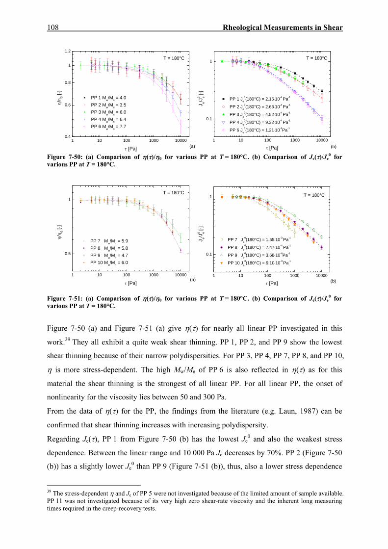
108 Rheological Measurements in Shear
Figure 7-50: (a) Comparison of η(τ)/η0 for various PP at T = 180°C. (b) Comparison of Je(τ)/Je
0 for various PP at T = 180°C.
Figure 7-51: (a) Comparison of η(τ)/η0 for various PP at T = 180°C. (b) Comparison of Je(τ)/Je
0 for various PP at T = 180°C.
Figure 7-50 (a) and Figure 7-51 (a) give η(τ) for nearly all linear PP investigated in this
work.39 They all exhibit a quite weak shear thinning. PP 1, PP 2, and PP 9 show the lowest
shear thinning because of their narrow polydispersities. For PP 3, PP 4, PP 7, PP 8, and PP 10,
η is more stress-dependent. The high Mw/Mn of PP 6 is also reflected in η(τ) as for this
material the shear thinning is the strongest of all linear PP. For all linear PP, the onset of
nonlinearity for the viscosity lies between 50 and 300 Pa.
From the data of η(τ) for the PP, the findings from the literature (e.g. Laun, 1987) can be
confirmed that shear thinning increases with increasing polydispersity.
Regarding Je(τ), PP 1 from Figure 7-50 (b) has the lowest Je0 and also the weakest stress
dependence. Between the linear range and 10 000 Pa Je decreases by 70%. PP 2 (Figure 7-50
(b)) has a slightly lower Je0 than PP 9 (Figure 7-51 (b)), thus, also a lower stress dependence
39 The stress-dependent η and Je of PP 5 were not investigated because of the limited amount of sample available. PP 11 was not investigated because of its very high zero shear-rate viscosity and the inherent long measuring times required in the creep-recovery tests.
1 10 100 1000 10000
0.5
1
PP 7 Mw/Mn = 5.9 PP 8 Mw/Mn = 5.8 PP 9 Mw/Mn = 4.7 PP 10 Mw/Mn = 6.0
η/η
0 [-]
τ [Pa]
T = 180°C
(a)1 10 100 1000 10000
0.1
1
PP 7 Je0(180°C) = 1.55⋅10-3 Pa-1
PP 8 Je0(180°C) = 7.47⋅10-4 Pa-1
PP 9 Je0(180°C) = 3.68⋅10-4Pa-1
PP 10 Je0(180°C) = 9.10⋅10-3 Pa-1
J e/J0 e [-
]
τ [Pa]
T = 180°C
(b)
1 10 100 1000 100000.4
0.6
0.8
1
1.2
PP 1 Mw/Mn = 4.0 PP 2 Mw/Mn = 3.5 PP 3 Mw/Mn = 6.0 PP 4 Mw/Mn = 6.4 PP 6 Mw/Mn = 7.7
η/η
0 [-]
τ [Pa]
T = 180°C
(a)1 10 100 1000 10000
0.1
1
PP 1 Je0(180°C) = 2.15⋅10-4 Pa-1
PP 2 Je0(180°C) = 2.66⋅10-4 Pa-1
PP 3 Je0(180°C) = 4.52⋅10-4 Pa-1
PP 4 Je0(180°C) = 9.32⋅10-4 Pa-1
PP 6 Je0(180°C) = 1.21⋅10-3Pa-1
J e/J0 e [-
]
τ [Pa]
T = 180°C
(b)

Rheological Measurements in Shear
109
of Je. For the materials PP 2 and PP 9 at a stress of 10 000 Pa Je is only 23% and 19% of Je0,
respectively. The stress dependence of Je for PP 3 is similar to that for PP 2 and PP 9,
however, from the value of Je0 a higher stress dependence was expected.
In the order PP 8, PP 10 (both Figure 7-51 (b)), PP 4 to PP 6 (both Figure 7-50 (b)) Je0
increases. The stress dependence of Je for these materials also increases in that order. For
these materials Je decreases from the linear regime to 10 000 Pa by about 85 to 90%. The
highest stress dependence of all linear PP is observed for the PP 7 (Figure 7-51 (b)) which
also has the highest Je0. As discussed in Chapter 7.2.2 and Appendix 12.8 the origin of the
high Je0 for PP 7 remains unclear.
The onset of nonlinearity lies at around 20 to 30 Pa for all linear PP, and thus, at lower
stresses than for the linear mLLDPE and the LCB-mLLDPE. For the linear PP, the decrease
of Je between the linear regime and the highest stress measured is comparable to that of the
LCB-mLLDPE and the LDPE; their Je0 lie in the same order of magnitude between 2·10-4 and
2·10-3 Pa-1, too.
Summarizing the results for the linear PP, the same outcome is found as for the PE, namely
Je(τ) reacts more sensitively to increasing stress than η(τ) and the stress dependence becomes
stronger the higher Je0 gets. The only exception represents PP 3 for which a higher stress
dependence of Je0 is expected.
Figure 7-52: (a) Comparison of η(τ)/η0 for linear PP and LCB-PP at T = 180°C. (b) Comparison for Je(τ)/Je
0 of linear PP and LCB-PP at T = 180°C.
Figure 7-52 (a) and Figure 7-52 (b) give η(τ) and Je(τ) for PP 1, PP 6, and the LCB-PP. The
LCB-PP exhibits a very pronounced stress dependence of η. At 10 000 Pa η is 20% of η0 and
the onset of the nonlinear regime lies at around 20 Pa. Thus, the shear thinning is even higher
than for LDPE-tub 4 and LDPE-aut 2 presented in Figure 7-49 (a). In addition, the stress
1 10 100 1000 100000.1
1
PP 1 Mw/Mn = 4.0 PP 6 Mw/Mn = 7.7 LCB-PP Mw/Mn = 22
η/η
0 [-]
τ [Pa]
T = 180°C
(a)1 10 100 1000 10000
0.1
1
PP 1 Je
0(180°C) = 2.15⋅10-4 Pa-1
PP 6 Je
0(180°C) = 1.21⋅10-3 Pa-1
LCB-PP Je
0(180°C) = 2.66⋅10-2 Pa-1
J e/J0 e [-
]
τ [Pa]
T = 180°C
(b)

110 Rheological Measurements in Shear
dependence of Je of the LCB-PP is the strongest of all materials investigated. Je at 3000 Pa is
almost 95% lower than Je0 and the onset of the nonlinear regime is already at 10 Pa.
7.2.6. Discussion: Stress Dependence of Je and η For all PE and PP investigated, a stronger stress dependence of Je(τ) compared to η(τ) is
observed. For these findings, a physical explanation has to be given.
It is commonly known that MMD (e.g. Laun, 1987) and LCB (e.g. Wood-Adams et al., 2000)
have a strong influence on the shear-thinning behaviour. A higher Mw/Mn as well as the
introduction of long-chain branches increase the stress dependence of η, whereas Mw does not
determine the shear thinning properties (e.g. Schwarzl, 1990). Concerning the influence of
MMD and LCB on the stress dependence of Je little is known.
According to Graessley (1974) the effect of polydispersity on η(τ) or η(γ& ) and Je(τ) or Je(γ& )
can be explained by disentanglement mechanisms. The longest molecules contribute the
longest relaxation times to the linear viscoelastic spectrum, and entanglements are released
from larger molecules at lower shear rates (stresses) than for smaller molecules. The long
relaxation time processes are, therefore, removed, progressively reducing the width of the
relaxation time spectrum with increasing stress or shear rate and tending thereby to reduce
η(τ) or η(γ& ) and Je(τ) or Je(γ& ).
Papers of Agarwal and Plazek (1977) and Plazek et al. (1979) on LDPE and HDPE confirm
the results of this work as they found a shift of the onset of the linear regime to lower stresses
as Je0 increased, too. The findings of Patham and Jayaraman (2005) on three ethylene-octene-
copolymers cannot be confirmed at the first glance. They assume a stronger stress
dependence of Je for linear materials than for long-chain branched ones. However, as already
shown in the literature section, all three of the mLLDPE investigated by them contain long-
chain branches as confirmed by the rheological and molecular data given in the article.
Therefore, from the results of the work of Patham and Jayaraman it is also confirmed that the
higher Je0 the stronger is the stress dependence of Je. In the stress regime of 5 to 10 000 Pa Je
decreased by 75% (Je0 = 4.1·10-4 Pa-1), 83% (Je
0 = 5.3·10-4 Pa-1), and 90% (Je0 = 5.8·10-4 Pa-1)
corresponding to the range found in this work.
Concerning a comparison between η(τ) and Je(τ) Plazek and O´Rourke (1971) and Agarwal
and Plazek (1977) showed for anionic PS and PS-blends (at T > Tg) and for LDPE,
respectively, that the onset of the nonlinear regime lies for η at higher shear stresses than for
Je. For PS in the stress range of 130 – 850 Pa Je decreased by about the fivefold, whereas, η is

Rheological Measurements in Shear
111
lowered only by 5%. For LDPE at the smallest stress investigated (60 Pa) Je0 is hardly
reached, whereas η0 can be determined at stresses below 200 Pa.
An explanation for the higher nonlinearity of Je compared to η and for the increasing stress
dependence of Je with increasing Je0 can be given from considerations on the entanglement
network. During a creep experiment at low stresses the entanglement network is orientated.
Even at low stresses, disentanglement occurs, but the entanglements can form again at these
low stresses. Thus, in the linear stress regime an equilibrium state between entanglement loss
and formation is assumed. The molecules reach their maximum stretch between the
entanglements at the end of the experiment in the steady state. Only when starting the
recovery experiment in this state of full orientation Je0 is measured. At higher creep stresses,
however, not only an orientation of the network takes place but also disentanglement plays a
decisive role. This means that due to the loss of entanglements, the entanglement network
stores a lower amount of elastic energy, and thus, Je becomes smaller. This picture is
consistent with the model of Graessley (1974) who explains the stress dependence of η and Je
by disentanglement effects, too, and predicts the loss of long relaxation times from long
and/or branched at high creep stresses.
Expressing η0 by the relaxation spectrum it can be seen that the contribution of the relaxation
strengths gi to η0 is proportional to their product with the relaxation times τi.
∑=
=n
iiig
10 τη (7.6)
To Je0, however, the contribution of the relaxation strength is approximately proportional to
the product of relaxation strength with the relaxation time squared. This means that the longer
relaxation times contribute more to Je0 compared to η0. However, from the relationship of Je
0
with the relaxation spectrum this cannot obviously be seen.40
2
1
1
2
0
⎟⎠
⎞⎜⎝
⎛=
∑
∑
=
=
n
iii
n
iii
e
g
gJ
τ
τ (7.7)
The short and/or linear molecules with the short relaxation times do not have as many
entanglements as the long and/or branched molecules. Thus, in a creep experiment at a high
creep stress the long and/or branched molecules can lose more entanglements, and therefore,
40 In Figure 12-17 of Appendix 12.5, the contributions of the relaxation times τi to η0 and Je
0 are presented. For the interpretation of the nonlinear behaviour it has to be assumed that Equation 7.6 and Equation 7.7 that define the linear steady-state quantities η0 and Je
0 are valid in the nonlinear stress regime for the calculation of η and Je, too.
112 Rheological Measurements in Shear
the relaxation times of the long and/or branched molecules are affected more by the nonlinear
creep stress leading to a more pronounced nonlinearity in η and Je compared to linear
materials. As the long relaxation times mainly contribute to Je0 it is comprehensible that Je
decreases stronglier with increasing stress than η. The formation of new entanglements on
long and/or branched molecules is less probable than on short molecules, too. The lower
mobility of the long molecules reduces the probability for re-entanglement.
In other rheological experiments the stronger influence of the long relaxation times on
elasticity than on viscosity becomes visible, too. In the dynamic-mechanical experiments the
loss modulus G´´ corresponds to the viscous properties and the storage modulus G´ to the
elastic properties. It can be observed that G´´ reaches the terminal slope of 1 at higher angular
frequencies than G´ the terminal slope of 2.
The finding of the same shape of Je(τ) independent of temperature and the existence of
mastercurves for Je(τ) has to be discussed. To the author´s knowledge, the stress dependence
of Je at different temperatures has been investivagated in the literature only for a linear PS by
Plazek and O´Rourke (1971). They found that Je is the same at different temperatures when
the stresses are the same. Je(τ) at different temperatures for thermorheologcially complex
materials are not reported and also the finding of Je0 being temperature-dependent for these
polymers is new. Therefore, an explanation for the independence of the shape of Je(τ) from
temperature cannot be found in the literature.
For the comparison of the different PE and PP investigated Je(τ) was normalized by Je0. The
quantity Je(τ)/Je0 is a measure for the nonlinear portion of the steady-state elastic compliance
and can be compared to the damping function h(γ) that is equivalent to the strain-dependent
part of the nonlinear shear relaxation modulus G(t,γ) when separability of strain and time is
assumed. G(t,γ) is defined as the linear shear relaxation modulus G(t) times h(γ).
)()(),( γγ htGtG = (7.8)
According to Wagner (1976), h(γ) reflects the disentanglement of the polymer network with
increasing deformation. The damping function is reported to be independent of temperature
for LDPE (Wagner and Laun, 1978), for linear PS (Archer, 1999), and for branched PS
(Hepperle and Münstedt, 2006). When similarities between the temperature-independent h(γ)
and Je(τ)/Je0 are assumed the temperature-independent shape of Je(τ) might seem less
surprising.
However, for the thermorheologically complex materials the result of a temperature-
independent shape of Je(τ) still seems remarkable because the shape of the relaxation spectra

Rheological Measurements in Shear
113
proved to be temperature-dependent. This temperature dependence of the spectra is caused by
the temperature dependence of the entanglement network. The number of entanglement
points is decisive for the number of orientated segments at the end of the creep experiment,
which contribute to the value of Je0. Due to the normalization by Je
0, the curve of Je(τ)/Je0,
however, does not reflect the total number of entanglement points but its shape characterizes
the change of the entanglement network by the applied stress. Therefore, Je(τ)/Je0 displays the
characteristic of disentanglement independent of temperature.

114 Rheological Measurements in Elongation
8. Rheological Measurements in Elongation
As presented in Chapter 5.3 two different types of measurements can be performed with the
MTR. Stressing experiments are the classical method often performed in the literature. Creep-
recovery experiments are not very common but are the main test method used in this work for
the characterization in elongation. In this chapter, the stressing experiments are discussed first.
Afterwards the results from the creep experiments are presented that can be compared to
those from the stressing tests. The main part is the presentation of the recovery experiments,
which give the elastic behaviour. The elastic properties are analyzed with respect to the
molecular structure of the materials and compared to the viscous properties.
Tensile experiments on mLLDPE cannot be performed as their viscosities and elasticities are
too small. Measurements of low viscous and low elastic materials are prone to
inhomogeneous sample deformation and buoyancy effects.
8.1. Stressing Experiments
In Figure 8-1 the results of the stressing experiments for LDPE-tub 4 and LDPE-aut 2
performed at 170°C are presented. Both materials exhibit a very pronounced strain hardening,
which increases with increasing strain rate. This behaviour is as expected from the literature
for LDPE (e.g. Gabriel and Münstedt, 2003). In addition, the threefold value of the linear
start-up viscosity in shear 3 η0(t) is plotted. The accordance of shear and elongational data is
not satisfactory. The deviation at a time of 100 s is 40% for LDPE-tub 4 and 65% for LDPE-
aut 2. An explanation for this unexpected behaviour is given in Appendix 12.12.
Figure 8-1: Transient tensile viscosities μ(t) at different strain rates ε& for (a) LDPE-tub 4 and (b) LDPE-aut 2.
1 10 100 1000
105
106
3 η0(t)
0.001 s-1
0.003 s-1 0.01 s-1
0.03 s-1
0.1 s-1
εH = 0.3 s-1
μ(t)
[Pa
s]
t [s]
LDPE-tub 4T = 170°C
.
(a)
εH = 3.8
1 10 100 1000
105
106
εH = 3.9
3 η0(t)
LDPE-aut 2T = 170°C
εH = 0.3 s-1 0.1 s-1
0.005 s-1 0.01 s-1 0.03 s-1
0.003 s-1
μ(t)
[Pa
s]
t [s]
.
(b)

Rheological Measurements in Elongation
115
The LCB-mLLDPE 3, which was investigated at 150°C, exhibits weaker strain hardening
than the LDPE that increases with decreasing strain rate, first (see Figure 8-2). At the lowest
elongational rate measured, however, the strain hardening decreases again. In the literature,
for LCB-mLLDPE similar findings are reported (Gabriel et al., 2002, Malmberg et al., 2002).
For the LCB-mLLDPE 3 the deviation between the envelope of the elongational
measurements and 3 η0(t) at 10 s is 25%, and thus, smaller than for the LDPE.
1 10 100
105
106
3 η0(t)
0.03s-1
0.05 s-1
0.1 s-1
0.3 s-1
μ(t)
[Pa
s]
t [s]
LCB-mLLDPE 3T = 150°C
1.0 s-1ε =.
εH = 3.7
Figure 8-2: Transient tensile viscosities μ(t) at different strain rates ε& for LCB-mLLDPE 3.
The stressing experiments of PP 10 and LCB-PP at 180°C are given in Figure 8-3 (a) and
Figure 8-3 (b). The linear PP 10 shows no strain hardening, the strain hardening of the LCB-
PP is very pronounced and even stronger than for the LDPE.41 As only three elongational
rates are measured an interpretation of the strain-hardening behaviour from the stressing
experiments is difficult. However, Stange (2006) also investigated this LCB-PP and found an
increasing strain hardening with increasing strain rate.
There is a deviation between the envelope of the elongational measurements and 3 η0(t) of
about 10% at 10 s for PP 10 and of about 20% at 10 s for LCB-PP, too.
41 The measurement for the LCB-PP at ε& = 0.001 s-1 does not show strain hardening, because strain hardening is expected at Hencky strains higher than 1 that cannot be experimentally reached for this elongational rate.

116 Rheological Measurements in Elongation
Figure 8-3: Transient tensile viscosities μ(t) at different strain rates ε& for (a) PP 10 and (b) LCB-PP (Wolff, 2008).
8.2. Creep-Recovery Experiments
Steady-state viscosities in elongation μs can be determined from the creep experiments. These
viscosities can be compared to the viscosities from the stressing experiments at long
measuring times when a stationary value has been attained because a stationary value of
viscosity in the stressing experiment also involves a constant stress.
In the recovery tests, the steady-state elastic tensile compliances De were determined.
The stress dependence of μs and De can be compared with respect to molecular structure of
the materials investigated. Furthermore, also a comparison between stress-dependent data of
μs and De with those of η and Je can be made.
8.2.1. Viscous Properties
In Figure 8-4, Figure 8-5, and Figure 8-6, the stationary viscosities of the creep and stressing
tests are plotted as a function of stress σ for LDPE-tub 4, LDPE-aut 2, and LCB-mLLDPE 3.
These viscosities are determined as explained in Chapter 5.3.4 and are average values of at
least three measurements.42 The values of μs from the stressing experiments are the maximum
values of μ(t) at long measuring times.
A ratio of three should be valid between the linear steady-state tensile viscosities μ0 and 3 η0.
The validity of this relationship has been shown for several linear and long-chain branched
polymers, such as polystyrene (Münstedt, 1975), polyethylene (e.g. Meissner, 1972, Laun and
42 In Chapter 5.3.4, an example for the proof of a steady-state in the creep experiment is given, too.
1 10 100
5x10⁴
105
1.5x10⁵
2x10⁵
2.5x10⁵
3 η0(t)
0.01 s-10.03 s-1
µ(t)
[Pa
s]
t [s]
PP 10T = 180°C
0.3 s-1ε =.
(a)
εH = 2.4
1 10 100 1000 10000104
105
106
3 η0(t)
0.001 s-1
0.03 s-1LCB-PPT = 180°CεH = 3.6
µ(t)
[Pa
s]
t [s]
ε = 0.3 s-1.
(b)

Rheological Measurements in Elongation
117
Münstedt, 1978, Münstedt and Laun, 1979, Münstedt and Laun, 1981, Münstedt et al., 1998,
Münstedt and Auhl, 2005) and polypropylene (Auhl et al., 2004).
For LDPE-tub 4, a very good coincidence of μs from creep and stressing experiments is found.
At the lowest creep stress applied (500 Pa) a viscosity in agreement to the threefold value of
η0 is measured. Only at the stresses of approximately 26 000 Pa and 74 000 Pa correlating to
strain rates of 0.03 and 0.01 s-1 the viscosities from the stressing experiments lie below the
values of the creep experiments, because of missing stationarity in the stressing test.43
For all materials investigated, at higher stresses (10 – 100 kPa) higher Hencky strains (3 - 4)
are necessary to reach a stationary state, whereas at the lowest stresses measured (0.5 – 2 kPa)
lower Hencky strains (0.8 – 1.5) are sufficient.
103 104 105
106
107
LDPE-tub 4T = 170°C
μ s [Pa
s]
σ [Pa]
μs from stressing test
μs from creep test
3 η0
Figure 8-4: Steady-state elongational viscosity μs as a function of stress for LDPE-tub 4.
For LDPE-aut 2, μs from creep and stressing experiments show a good agreement, too (see
Figure 8-5). Also for this material at the intermediate strain rates of 0.03 to 0.005 s-1 a
stationary state cannot be reached in the stressing experiment, and therefore, the values for μs
are too small. For this material, μs measured at the lowest stress of 750 Pa and the lowest
strain rate of 0.001 s-1 is about 35% higher than 3 η0. Also the deviation of the linear start-up
viscosity in shear 3 η0(t) from the envelope of the curves of the stressing experiment is higher
for LDPE-aut 2 than for LDPE-tub 4.
43 Münstedt et al. (1998) and Münstedt and Auhl (2005) report that the steady state is reached at smaller Hencky strains in the creep test than in the stressing experiment.

118 Rheological Measurements in Elongation
103 104 105
106
107
LDPE-aut 2T = 170°C
3 η0
μ s [Pa
s]
σ [Pa]
μs from stressing test
μs from creep test
Figure 8-5: Steady-state elongational viscosity μs as a function of stress for LDPE-aut 2. For LCB-mLLDPE 3 (Figure 8-6), the μs of stressing and creep experiments coincide at low
stresses. The deviation between μs measured at the lowest stresses and 3 η0 is about 12%. As
in the stressing experiments for elongational rates of 0.05 s-1 and higher, no steady states
could be reached no values for μs at higher creep stresses determined from the stressing
experiments are plotted in Figure 8-6.
103 104 105
105
1.5x10⁵
2x10⁵
2.5x10⁵
3x10⁵
LCB-mLLDPE 3T = 150°C
3 η0
μ s [Pa
s]
σ [Pa]
μs from stressing test
μs from creep test
Figure 8-6: Steady-state elongational viscosity μs as a function of stress for LCB-mLLDPE 3.

Rheological Measurements in Elongation
119
For the PP 10 (Figure 8-7), which exhibits no strain hardening, μs determined in the creep and
stressing experiments coincide quite well. The deviation of the elongational viscosities μs at
low stresses from 3 η0 is approximately 5%, which lies within the accuracy of the
measurement.
100 1000 10000105
1.2x10⁵
1.4x10⁵
1.6x10⁵
1.8x10⁵
2x10⁵
3 η0
μs from stressing test μs from creep test
µ s [Pa
s]
σ [Pa]
PP 10T = 180°C
Figure 8-7: Steady-state elongational viscosity μs as a function of stress for PP 10 (Wolff et al., 2010).
The values of μs determined in the creep experiments for the LCB-PP are listed in Table 8-1.
μs at lower creep stresses cannot be measured as in the accessible range of Hencky strains a
steady state in the creep experiment cannot be obtained. No values for μs from the stressing
experiments can be determined also because of missing stationarity.
Table 8-1: Steady-state elongational viscosities μs measured at creep stresses between 5000 and 50 000 Pa for the LCB-PP (Wolff, 2008).
σ [Pa] 5000 10 000 20 000 30 000 50 000
μs [Pa s] (1.91±0.18)·106 (2.62±0.18)·106 (3.66±0.23)·106 (3.64±0.17)·106 (3.74±0.14)·106
A comparison of the elongational viscosities as a function of σ for the different materials is
given in Figure 8-8 which shows μs normalized by 3 η0 vs. σ.44
44 The different measuring temperatures are not expected to influence the interpretation of the results, because the shape of μs(σ) is the same independent of temperature. Machui (2009) showed for an LLDPE and a PS at temperatures between 160°C and 180°C that the same shift factor is valid for μs(σ) in the range of 1000 to 50 000 Pa. According to the time-temperature-superposition principle, also the temperature dependence of η and μs are the same.

120 Rheological Measurements in Elongation
For PP 10 strain hardening is missing and μs is independent of σ in the range of 500 to
20 000 Pa. At the highest stresses measured, μs decreases with increasing stress comparable to
a shear-thinning behaviour. All other materials containing LCB show strain hardening. The
strain hardening of LCB-mLLDPE 3 is weak compared to the LDPE and the LCB-PP. For the
LCB-PP the strain hardening is the strongest with μs being more than 20 times stronger than
3 η0. The strain hardening of LDPE-aut 2 is more pronounced than for LDPE-tub 4. Also
Yamaguchi and Takahashi (2001) and Wagner et al. (2003) report higher strain hardening for
autoclave types than for tubular resins.
1000 10000 100000
1
10
T = 170°C LDPE-tub 4 LDPE-aut 2
T = 150°C LCB-mLLDPE 3
T = 180°C PP10 LCB-PP
μ s/3η 0 [-
]
σ [Pa]
Figure 8-8: Elongational viscosity μs normalized by 3 η0 as a function of stress for LDPE-tub 4, LDPE-aut 2, LCB-mLLDPE 3, PP 10, and LCB-PP.
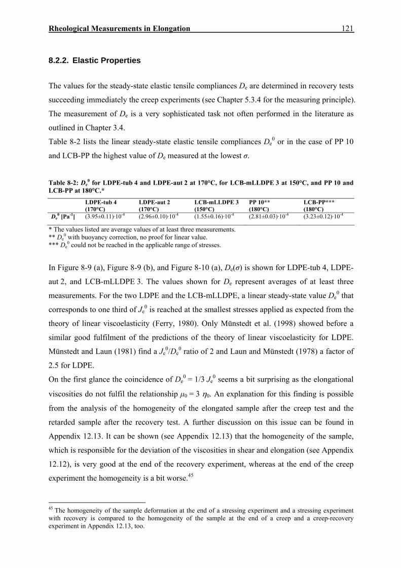
Rheological Measurements in Elongation
121
8.2.2. Elastic Properties
The values for the steady-state elastic tensile compliances De are determined in recovery tests
succeeding immediately the creep experiments (see Chapter 5.3.4 for the measuring principle).
The measurement of De is a very sophisticated task not often performed in the literature as
outlined in Chapter 3.4.
Table 8-2 lists the linear steady-state elastic tensile compliances De0 or in the case of PP 10
and LCB-PP the highest value of De measured at the lowest σ.
Table 8-2: De
0 for LDPE-tub 4 and LDPE-aut 2 at 170°C, for LCB-mLLDPE 3 at 150°C, and PP 10 and LCB-PP at 180°C.*
LDPE-tub 4 (170°C)
LDPE-aut 2 (170°C)
LCB-mLLDPE 3 (150°C)
PP 10** (180°C)
LCB-PP*** (180°C)
De0 [Pa-1] (3.95±0.11)·10-4 (2.96±0.10)·10-4 (1.55±0.16)·10-4 (2.81±0.03)·10-4 (3.23±0.12)·10-4
* The values listed are average values of at least three measurements. ** De
0 with buoyancy correction, no proof for linear value. *** De
0 could not be reached in the applicable range of stresses.
In Figure 8-9 (a), Figure 8-9 (b), and Figure 8-10 (a), De(σ) is shown for LDPE-tub 4, LDPE-
aut 2, and LCB-mLLDPE 3. The values shown for De represent averages of at least three
measurements. For the two LDPE and the LCB-mLLDPE, a linear steady-state value De0 that
corresponds to one third of Je0 is reached at the smallest stresses applied as expected from the
theory of linear viscoelasticity (Ferry, 1980). Only Münstedt et al. (1998) showed before a
similar good fulfilment of the predictions of the theory of linear viscoelasticity for LDPE.
Münstedt and Laun (1981) find a Je0/De
0 ratio of 2 and Laun and Münstedt (1978) a factor of
2.5 for LDPE.
On the first glance the coincidence of De0 = 1/3 Je
0 seems a bit surprising as the elongational
viscosities do not fulfil the relationship μ0 = 3 η0. An explanation for this finding is possible
from the analysis of the homogeneity of the elongated sample after the creep test and the
retarded sample after the recovery test. A further discussion on this issue can be found in
Appendix 12.13. It can be shown (see Appendix 12.13) that the homogeneity of the sample,
which is responsible for the deviation of the viscosities in shear and elongation (see Appendix
12.12), is very good at the end of the recovery experiment, whereas at the end of the creep
experiment the homogeneity is a bit worse.45
45 The homogeneity of the sample deformation at the end of a stressing experiment and a stressing experiment with recovery is compared to the homogeneity of the sample at the end of a creep and a creep-recovery experiment in Appendix 12.13, too.

122 Rheological Measurements in Elongation
Figure 8-9: Steady-state elastic tensile compliance De as a function of stress for (a) LDPE-tub 4 and (b) LDPE-aut 2.
Figure 8-10: Steady-state elastic tensile compliance De as a function of stress for (a) LCB-mLLDPE 3 and (b) LCB-PP (Wolff, 2008).
De0 of LCB-PP cannot be reached in the accessible range of stresses, as presented in Figure
8-10 (b). The De measured lie far away from the linear stress regime. A very cautious
extrapolation of the De values would suggest that De0 would be reached at σ smaller than
100 Pa.
In the case of PP 10, the recovery tests are superimposed by a buoyancy effect due to
differences in the densities of the sample and the silicone oil at the measuring temperature. As
presented in Figure 8-11, the actually measured De are too small.46 The buoyancy effect can
46 The influence of buoyancy is significant at small stresses and almost negligible at high stresses. Particularly materials with low elasticities and viscosities are prone to superimposing effects resulting from differences in the density of the sample and the silicone oil (Wolff, 2008, Wolff et al., 2010).
1000 10000 10000010-5
10-4
LDPE-tub 4T = 170°C
De [P
a-1]
σ [Pa]
1/3 J0e
(a)1000 10000 100000
10-5
10-4
De [P
a-1]
σ [Pa]
1/3 J0e
LDPE-aut 2T = 170°C
(b)
1000 10000 10000010-5
10-4
LCB-mLLDPE 3T = 150°C
De [P
a-1]
σ [Pa]
1/3 J0e
(a)
1000 10000 10000010-5
10-4
10-3
10-2
1/3 J 0e
De [P
a-1]
σ [Pa]
LCB-PPT = 180°C
(b)
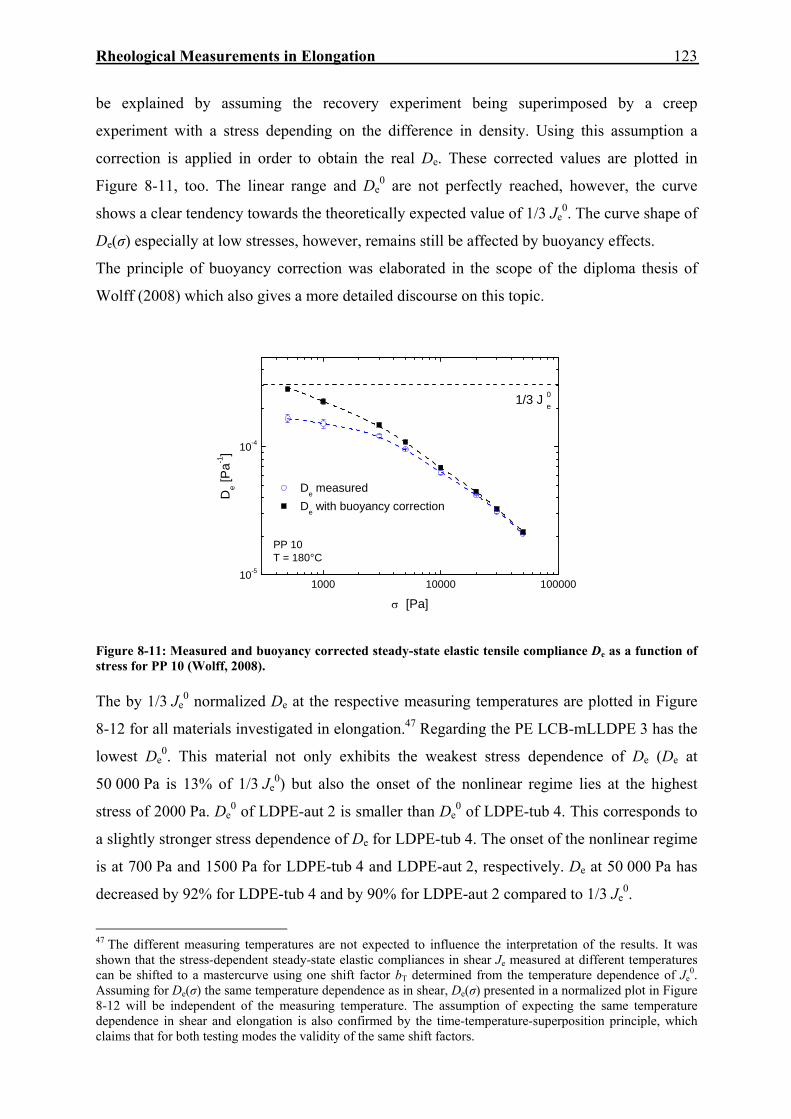
Rheological Measurements in Elongation
123
be explained by assuming the recovery experiment being superimposed by a creep
experiment with a stress depending on the difference in density. Using this assumption a
correction is applied in order to obtain the real De. These corrected values are plotted in
Figure 8-11, too. The linear range and De0 are not perfectly reached, however, the curve
shows a clear tendency towards the theoretically expected value of 1/3 Je0. The curve shape of
De(σ) especially at low stresses, however, remains still be affected by buoyancy effects.
The principle of buoyancy correction was elaborated in the scope of the diploma thesis of
Wolff (2008) which also gives a more detailed discourse on this topic.
1000 10000 10000010-5
10-4
De measured De with buoyancy correction
De [P
a-1]
σ [Pa]
PP 10T = 180°C
1/3 J 0e
Figure 8-11: Measured and buoyancy corrected steady-state elastic tensile compliance De as a function of stress for PP 10 (Wolff, 2008). The by 1/3 Je
0 normalized De at the respective measuring temperatures are plotted in Figure
8-12 for all materials investigated in elongation.47 Regarding the PE LCB-mLLDPE 3 has the
lowest De0. This material not only exhibits the weakest stress dependence of De (De at
50 000 Pa is 13% of 1/3 Je0) but also the onset of the nonlinear regime lies at the highest
stress of 2000 Pa. De0 of LDPE-aut 2 is smaller than De
0 of LDPE-tub 4. This corresponds to
a slightly stronger stress dependence of De for LDPE-tub 4. The onset of the nonlinear regime
is at 700 Pa and 1500 Pa for LDPE-tub 4 and LDPE-aut 2, respectively. De at 50 000 Pa has
decreased by 92% for LDPE-tub 4 and by 90% for LDPE-aut 2 compared to 1/3 Je0.
47 The different measuring temperatures are not expected to influence the interpretation of the results. It was shown that the stress-dependent steady-state elastic compliances in shear Je measured at different temperatures can be shifted to a mastercurve using one shift factor bT determined from the temperature dependence of Je
0. Assuming for De(σ) the same temperature dependence as in shear, De(σ) presented in a normalized plot in Figure 8-12 will be independent of the measuring temperature. The assumption of expecting the same temperature dependence in shear and elongation is also confirmed by the time-temperature-superposition principle, which claims that for both testing modes the validity of the same shift factors.

124 Rheological Measurements in Elongation
For PP 10, De0 is not reliably determined as on the one hand the buoyancy correction is
applied and on the other hand only the measurements at the lowest stress of 500 Pa give a De
close to 1/3 Je0. Between 500 and 50 000 Pa De decreases by 93%, an order of magnitude
comparable to the LDPE. The values of De measured for LCB-PP, which lie away from the
linear regime, suggest a much more pronounced stress dependence of De compared to PP 10.
It can be stated that the linear range of PP 10 extends to much higher stresses than the linear
range of the LCB-PP. Taking 1/3 Je0 as reference value De of the LCB-PP at 50 000 Pa is only
0.5% of the expected linear steady-state value. This findings can be explained by the high
Mw/Mn and the long-chain branches in the LCB-PP.48
Literature data on elasticity measured in elongation are scarce, so a comparison to literature
results is hardly possible. Only Münstedt and Laun (1981) report for various LDPE and
HDPE that the differences in recoverable strain between these materials become smaller with
increasing stress, indicating that materials with high recoverable strains in the linear stress
regime corresponding to high De0 show a more pronounced stress dependence.
1000 10000 100000
0.01
0.1
1
T = 170°C LDPE-tub 4 LDPE-aut 2
T = 150°C LCB-mLLDPE 3
T = 180°C PP 10* LCB-PP
De/1
/3J0 e [-
]
σ [Pa]
*buoyancy correction applied
Figure 8-12: De
0 normalized by 1/3 Je0 as a function of stress for LDPE-tub 4, LDPE-aut 2, LCB-
mLLDPE 3, PP 10, and LCB-PP.
For the PE and the PP, respectively, it is observed in shear rheology that the nonlinearity in
elasticity increases with increasing Je0. Regarding the PE also the stress dependence of De is
stronger the higher De0 (see Figure 8-12). The De
0 decrease in the order LDPE-tub 4, LDPE-
aut 2, and LCB-mLLDPE 3. Also the decrease in nonlinearity in De(σ) follows this order.
48 The differences in De(σ) between PP 10 and LCB-PP are significant, and thus, despite of the experimental difficulties in the tensile creep-recovery experiments of the PP the comparison of the data seems reasonable.
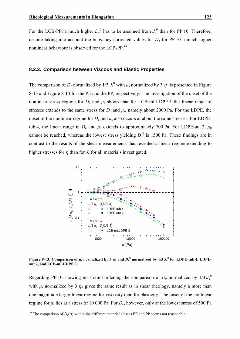
Rheological Measurements in Elongation
125
For the LCB-PP, a much higher De0 has to be assumed from Je
0 than for PP 10. Therefore,
despite taking into account the buoyancy corrected values for De for PP 10 a much higher
nonlinear behaviour is observed for the LCB-PP.49
8.2.3. Comparison between Viscous and Elastic Properties
The comparison of De normalized by 1/3 Je0 with μs normalized by 3 η0 is presented in Figure
8-13 and Figure 8-14 for the PE and the PP, respectively. The investigation of the onset of the
nonlinear stress regime for De and μs shows that for LCB-mLLDPE 3 the linear range of
stresses extends to the same stress for De and μs, namely about 2000 Pa. For the LDPE, the
onset of the nonlinear regime for De and μs also occurs at about the same stresses. For LDPE-
tub 4, the linear range in De and μs extends to approximately 700 Pa. For LDPE-aut 2, μ0
cannot be reached, whereas the lowest stress yielding De0 is 1500 Pa. These findings are in
contrast to the results of the shear measurements that revealed a linear regime extending to
higher stresses for η than for Je for all materials investigated.
1000 10000 100000
0.1
1
10
T = 170°C μs/3 η0 De/1/3 J0
e
LDPE-tub 4 LDPE-aut 2
T = 150°C μs/3 η0 De/1/3 J0
e
LCB-mLLDPE 3
μ s/3 η
0, De/1
/3 J
0 e [-]
σ [Pa]
Figure 8-13: Comparison of μs normalized by 3 η0 and De
0 normalized by 1/3 Je0 for LDPE-tub 4, LDPE-
aut 2, and LCB-mLLDPE 3.
Regarding PP 10 showing no strain hardening the comparison of De normalized by 1/3 Je0
with μs normalized by 3 η0 gives the same result as in shear rheology, namely a more than
one magnitude larger linear regime for viscosity than for elasticity. The onset of the nonlinear
regime for μs lies at a stress of 10 000 Pa. For De, however, only at the lowest stress of 500 Pa 49 The comparison of De(σ) within the different material classes PE and PP seems not reasonable.
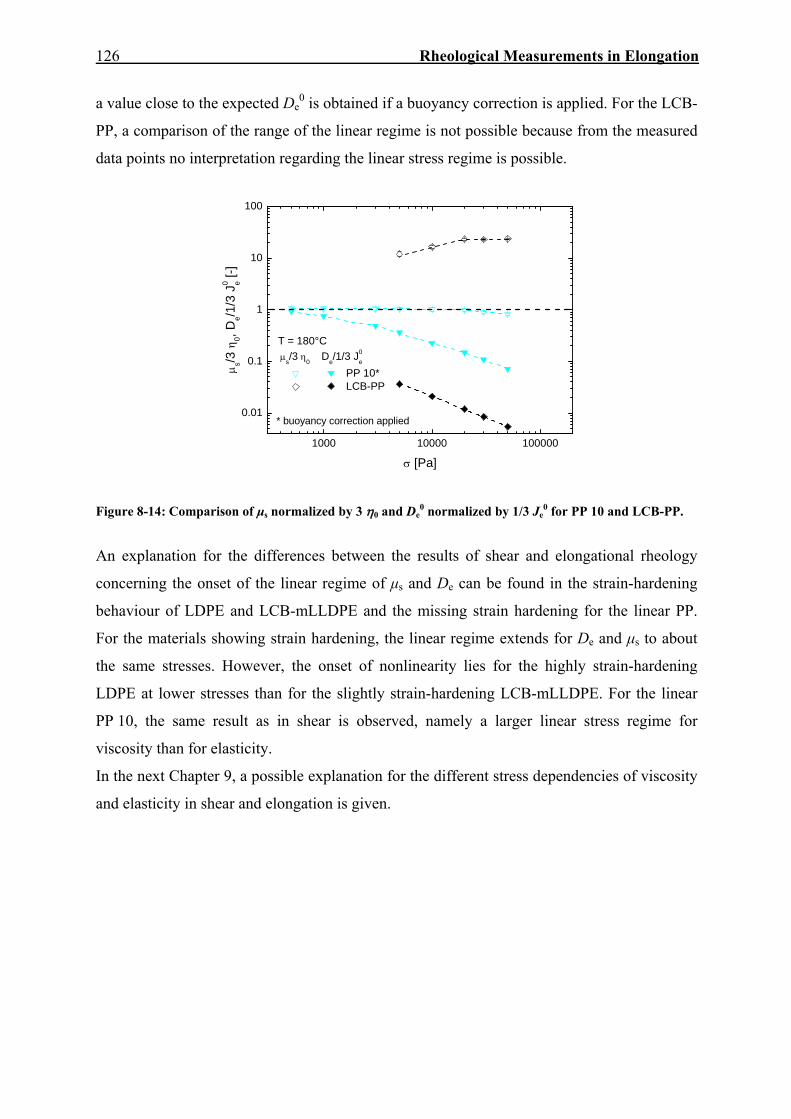
126 Rheological Measurements in Elongation
a value close to the expected De0 is obtained if a buoyancy correction is applied. For the LCB-
PP, a comparison of the range of the linear regime is not possible because from the measured
data points no interpretation regarding the linear stress regime is possible.
1000 10000 100000
0.01
0.1
1
10
100
T = 180°C μs/3 η0 De/1/3 J0
e PP 10* LCB-PP
μs/3
η0, D
e/1/3
J0 e [-
]
σ [Pa]
* buoyancy correction applied
Figure 8-14: Comparison of μs normalized by 3 η0 and De
0 normalized by 1/3 Je0 for PP 10 and LCB-PP.
An explanation for the differences between the results of shear and elongational rheology
concerning the onset of the linear regime of μs and De can be found in the strain-hardening
behaviour of LDPE and LCB-mLLDPE and the missing strain hardening for the linear PP.
For the materials showing strain hardening, the linear regime extends for De and μs to about
the same stresses. However, the onset of nonlinearity lies for the highly strain-hardening
LDPE at lower stresses than for the slightly strain-hardening LCB-mLLDPE. For the linear
PP 10, the same result as in shear is observed, namely a larger linear stress regime for
viscosity than for elasticity.
In the next Chapter 9, a possible explanation for the different stress dependencies of viscosity
and elasticity in shear and elongation is given.
Comparison of Rheological Properties in Shear and Elongation
127
9. Comparison of Rheological Properties in Shear and Elongation
This chapter presents a summary of the results of the previous Chapters 7.2 and 8 and gives a
comparison of the data from shear for η(τ) and Je(τ) with those from elongation for μs(σ) and
De(σ). Viscosity data in shear and elongation covering a wide range of stress as in this thesis
were so far presented exclusively by Münstedt (1975) and Laun and Münstedt (1978).
9.1. Stress-Dependent Viscosities and Steady-State Elastic Compliances in Shear and Elongation
In shear and elongational experiments two different kinds of stresses are applied, therefore,
for the comparison of the results of these two test types reference stresses have to be
calculated. The comparison of shear and tensile stresses bases on Mohr´s circle of stress (e.g.
Chou and Pagano, 1992). The maximum shear stress acting on the sample τxy,max is calculated
by:
22
max, 2 xyyx
xy τσσ
τ +⎟⎟⎠
⎞⎜⎜⎝
⎛ −±= (9.1)
σx and σy are the normal stresses acting in x- and y-direction, respectively. τxy denotes the
shear stress, corresponding to τ. In the case of shear deformation, σx and σy are negligibly
small; therefore, only τxy contributes to Equation (9.1).50 In the case of tensile deformation,
only a normal force in one direction σx or σy, depending on the definition of the coordinate
system, acts on the specimen, which corresponds to σ. τxy is zero. Thus, using Equation (9.1)
for tensile deformation τxy,max is 1/2 σ. τxy,max for shear deformation is simplyτ.
The shear viscosities η(τ) are multiplied by a factor of three according to the Trouton ratio in
order to make a comparison with the tensile viscosities possible.
The results of the measurement of 3 η(τ) and μs(1/2 σ) over the experimentally accessible
stress range are shown in Figure 9-1 (a), Figure 9-2 (a), Figure 9-3 (a), Figure 9-4 (a), and
Figure 9-5 (a) for LDPE-tub 4, LDPE-aut 2, LCB-mLLDPE 3, PP 10, and LCB-PP,
respectively.
50 For LDPE-tub 4 having the highest η0 of all materials investigated, a 4% higher shear stress is calculated by Equation (9.1) if the normal force acting on the sample, which is recorded throughout the measurement by the rheometer software, is not neglected. For materials with lower η0, the effect of normal force is by up to a factor of 10 smaller.

128 Comparison of Rheological Properties in Shear and Elongation
For the LDPE, the onset of the nonlinear stress regime occurs at approximately the same
stress for η and μs. For the LCB-mLLDPE, the onset of nonlinearity of μs lies at about one
order of magnitude higher stresses than of η, for the linear PP, this difference in the onset of
nonlinearity is even higher, presumably because of the absence of strain hardening. For the
LCB-PP, the onset of nonlinearity cannot be assessed as the linear stress range in elongation
lies at very small stresses that are not experimentally accessible.
Also in the literature, Münstedt (1975) reports for linear PS that the linear range in elongation
is larger by more than one order of magnitude compared to the linear range in shear. For the
investigated PS, the linear range of viscosity extends to approximately 1000 Pa in shear and
to approximately 50 000 Pa in elongation. This is in accordance to the findings on PP 10 and
LCB-mLLDPE 3 for which the onset of the nonlinear regime in shear lies at around 100 Pa,
whereas in elongation for PP 10 only at 500 Pa and for LCB-mLLDPE 3 at 1000 Pa and
2000 Pa viscosities close to 3 η0 are attained. In the case of LDPE-tub 4 and LDPE-aut 2,
there are hardly any differences between the onset of the nonlinear regime in shear and
elongation. This corresponds to published data of LDPE by Laun and Münstedt (1978) and
Münstedt (1981) that show linear ranges equal in shear and elongation.51
For PP 10 without strain hardening, the viscosity curves in shear and elongation display a
similar shape (Figure 9-4 (a)). The viscosity curve in elongation seems to be shifted by a
factor of 25 to higher stresses.
Figure 9-1: Comparison of (a) 3 η(τ) with μs(1/2 σ) and (b) 1/3 Je(τ) with De(1/2 σ) for LDPE-tub 4.
51 Laun and Münstedt (1978) and Münstedt (1981) do not present μs as a function of 1/2 σ but as a function of σ.
10 100 1000 10000 100000
105
106
3 η μs
3 η,
μs [P
a s]
τ, 1/2 σ [Pa]
LDPE-tub 4T = 170°C
3 η0
(a)
1 10 100 1000 10000 10000010-5
10-4
10-3
1/3 J0e
LDPE-tub 4T = 170°C
1/3 Je
De
1/3
J e, De [P
a-1]
τ, 1/2 σ [Pa] (b)

Comparison of Rheological Properties in Shear and Elongation
129
Figure 9-2: Comparison of (a) 3 η(τ) with μs(1/2 σ) and (b) 1/3 Je(τ) with De(1/2 σ) for LDPE-aut 2.
Figure 9-3: Comparison of (a) 3 η(τ) with μs (1/2 σ) and (b) 1/3 Je(τ) with De(1/2 σ) for LCB-mLLDPE 3.
Figure 9-4: Comparison of (a) 3 η(τ) with μs(1/2 σ) and (b) 1/3 Je(τ) with De(1/2 σ) for PP 10 (Wolff et al., 2010).
10 100 1000 10000 100000
105
106
3 η μs
3 η,
μs [P
a s]
τ, 1/2 σ [Pa]
LDPE-aut 2T = 170°C
3 η0
(a)
1 10 100 1000 10000 10000010-5
10-4
10-3
1/3 J0e
LDPE-aut 2T = 170°C
1/3 Je
De
1/3
J e, D
e [Pa
-1]
τ, 1/2 σ [Pa] (b)
1 10 100 1000 10000 100000
105
2x10⁵
3x10⁵
4x10⁵
3 η μs
3 η,
μs [P
a s]
τ, 1/2 σ [Pa]
LCB-mLLDPE 3T = 150°C
3 η0
(a)
1 10 100 1000 10000 10000010-5
10-4
10-3
1/3 J0e
LCB-mLLDPE 3 T = 150°C
1/3 Je
De
1/3
J e, De [P
a-1]
τ, 1/2 σ [Pa] (b)
1 10 100 1000 10000 100000
105
1.5x10⁵
2x10⁵
2.5x10⁵
3 η μs
3 η,
μs [P
a s]
τ, 1/2 σ [Pa]
PP 10T = 180°C
3 η0
(a)
1 10 100 1000 10000 10000010-5
10-4
10-3
PP 10T = 180°C
1/3 J0e
1/3 Je
De
1/3
J e, De [P
a-1]
τ, 1/2 σ [Pa] (b)

130 Comparison of Rheological Properties in Shear and Elongation
Figure 9-5: Comparison of (a) 3 η(τ) with μs(1/2 σ) and (b) 1/3 Je(τ) with De(1/2 σ) for LCB-PP (Wolff, 2008).
The results of the measurements of 1/3 Je(τ) and De(1/2 σ) over the experimentally accessible
stress range are shown in Figure 9-1 (b), Figure 9-2 (b), Figure 9-3 (b), Figure 9-4 (b), and
Figure 9-5 (b) for LDPE-tub 4, LDPE-aut 2, LCB-mLLDPE 3, PP 10, and LCB-PP,
respectively.
For all materials investigated, the linear range of De(1/2 σ) extends to higher stresses than the
linear range of 1/3 Je(τ). For the LCB-PP, this cannot be shown, as in the accessible range of
tensile stresses the De(1/2 σ) are much smaller than 1/3 Je0.
Even for the LDPE, the differences in the stresses at the onset of the nonlinear regime
between De(1/2 σ) and 1/3 Je(τ) are larger by more than one order of magnitude, whereas
between 3 η(τ) and μs(1/2 σ) hardly any difference is observed. Laun and Münstedt (1978)
and Münstedt et al. (1998) detect for LDPE qualitatively the same behaviour, namely a larger
linear range for De(σ) compared to Je(τ).
For all materials, can be observed that once the stress has exceeded the onset of nonlinearity
the decrease in De is more pronounced than in Je. For the LCB-PP, this can only be estimated
from the steeper slope of De(1/2 σ) compared to 1/3 Je(τ).
From the present results, no simple quantitative correlation can be established between the Je
and De outside the linear range. Laun and Münstedt (1978) drew the same conclusion for
LDPE.
1 10 100 1000 10000104
105
106
107
3 η μs
3 η
, μs [P
a s]
τ, 1/2 σ [Pa]
LCB-PPT = 180°C
3 η0
(a)1 10 100 1000 10000 100000
10-4
10-3
10-2
LCB-PPT = 180°C 1/3 J0
e
1/3 Je
De
1/3
J e, De [P
a-1]
τ, 1/2 σ [Pa] (b)

Comparison of Rheological Properties in Shear and Elongation
131
9.2. Discussion: Stress-Dependent Viscosities and Steady-State Elastic Compliances in Shear and Elongation
This chapter presents an approach for the interpretation of the different stress dependencies of
η, μs, Je, and De with respect to molecular structure.
In the literature, the molecular theories based on the so-called tube model, which Doi and
Edwards (1986) developed originally, offer a theoretical description for most of the
rheological findings on viscosity in shear and elongation in the linear and nonlinear
viscoelastic regime for polymers with different molecular structures. Concerning elastic
properties in shear, particularly the first normal stress difference could be successfully
described. Dealy and Larson (2006) give a comprehensive review on the development of the
tube models in the last decades and their capabilities in modelling experimental rheological
data. However, for linear and nonlinear elasticity in elongation the tube models do not offer to
the author´s knowledge a profound description of experimental rheological data. Therefore,
the present results can only be explained phenomenologically.
In elongation, the linear PP showing no strain hardening behaves similar as in shear, where a
larger linear regime and a weaker stress dependence for η than for Je was observed. In
addition, in elongation the linear regime for μs extends to higher stresses compared to De and
the stress dependence of De is much stronger compared to μs. For the long-chain branched
materials, however, the onset of the nonlinear regime for μs and De occurs at approximately
the same stresses. In Chapter 7.2.6, the assumption of changes in the entanglement network
that affect η and Je differently allowed an interpretation of the stress dependence of viscosity
and elasticity. For the linear PP in elongation, the same assumptions as outlined in Chapter
7.2.6 for the shear data are valid. However, the disentanglement processes in elongation start
at higher stresses because the elongational deformation leads to a more effective orientation
of the molecules that does not allow the molecules to disentangle at low stresses. Shear
deformation, however, cannot hinder the disentanglement at such an extent. If going to high
stresses, disentanglement becomes also important in elongation as the entanglements are
released leading to a decrease of μs and De with increasing stress. This means that higher
stresses are necessary to reach the nonlinear regime in elongation, but once the nonlinearity
threshold is exceeded a more effective orientation of the molecules and faster
disentanglement processes take place in elongation than in shear.
For the long-chain branched materials, other mechanisms in the entanglement network during
tensile creep experiments have to be assumed than for the linear polymers. It is known from
132 Comparison of Rheological Properties in Shear and Elongation
the tube models that in elongation the reaction of the entanglement network to the applied
stress is significantly different for long-chain branched and for linear molecules. For a
polymer with more than one branch point along the chain there is a portion of the molecule´s
backbone with no free ends that lies between the terminal branch points (inner segment). The
relaxation of the conformation and the movement of the polymer chain within these inner
segments obey different mechanisms as assumed for linear chains or free arms. The backbone
segments are expected to have great difficulty relaxing, and thus, to be especially slow in
relaxing. Furthermore, they are made responsible for the strain hardening in extensional flow.
Different relaxation mechanisms of linear and long-chain branched molecules are also a
presumption in theories that describe the elongational viscosity at a constant strain rate as a
function of time as the molecular stress function theory by Wagner (e.g. Wagner et al., 2000)
or the Pom-Pom model by the group of McLeish (see Dealy and Larson, 2006, for details).
The elongational stress orientates the network and the backbone of the molecules. However,
the long-chain branches of the molecules cannot easily disentangle leading to an orientation
of the molecule and to stresses on the backbone, that contribute to the strain-hardening
behaviour. A release of the stress of the molecule backbone is only possible by a withdrawl
and disentanglement of the arms at large deformations and/or high stresses.
For the long-chain branched materials, two regimes in μs can be distinguished. In the first
regime up to the maximum in strain hardening at around 10 000 Pa the long-chain branches
hinder the disentanglement processes to a great extend. Once the arms have disentangled,
after exceeding the maximum in strain hardening, in the second regime it is assumed that the
long-chain branched molecules behave similar to the linear molecules leading to decrease in
μs with increasing stress. However, there is also a loss of entanglements in the first regime
which is superimposed by the more pronounced strain-hardening effect. This disentanglement
in the first regime may lead, as in shear, to a decrease in the amount of energy that can be
stored in the network and, thereby, reduces De at much lower stresses than the decrease in μs
takes place.
A further interpretation of the differences between the stress-dependent behaviour of the
rheological quantities in shear and elongation for linear and long-chain branched materials
lies beyond the scope of this thesis. The qualitative and simple picture regarding changes in
the entanglement network used in this work does not allow a complete phenomenological
explanation of all the findings. To reconsider this picture the description of the experimental
data using constitutive equations basing on tube models may contribute to answer the

Comparison of Rheological Properties in Shear and Elongation
133
questions about the mechanisms of changes in the entanglement network and may offer a
quantitative description of the rheological measurements performed.
The group of Prof. Wagner (University Berlin) works on a theoretical description of the data
using the molecular stress function model (MSF-model) in the scope of a DFG project, which
also includes this thesis.

134 Summary and Outlook
10. Summary and Outlook
• Summary
In this thesis, rheological measurements in shear and elongational were performed in order to
investigate the viscous and elastic properties of polyolefin melts with different molecular
architectures in the linear and nonlinear stress regime. About the influence of molar mass Mw,
molar mass distribution (MMD), and long-chain branching (LCB) on viscosity extensive
knowledge is available. For the elastic properties, the literature is scarce and particularly
systematic studies are missing. In addition, the comparison of viscous and elastic properties in
shear and elongation is of interest, though, little is known from the literature. Therefore,
creep-recovery measurements in shear, which allow the determination of the viscosity η and
the elasticity, in terms of the steady-state elastic compliance Je, were applied to well
characterized polyethylenes and polypropylenes. By these means, correlations of the
molecular structure with the linear rheological quantities, zero shear-rate viscosity η0 and
linear steady-state elastic compliance Je0, as well as with the stress dependence of viscosity
and elasticity could be found. Additionally, for some materials the stress dependence of
steady-state tensile viscosities μs and steady-state elastic tensile compliances De was
determined using creep-recovery experiments in elongation. The results from shear and
elongational rheology were analyzed with respect to the molecular structure of the polyolefins.
Polyethylenes (mLLDPE, LCB-mLLDPE, and LDPE) and polypropylenes (linear iPP and
LCB-PP) were selected and thoroughly characterized using DSC, FT-IR, SEC-MALLS, and
dynamic-mechanical experiments. The molecular characterization is of great importance as
viscosity is highly influenced by molar mass and long-chain branching and elasticity is
mainly determined by polydispersity and long-chain branching. The dynamic-mechanical
measurements were presented in the plot of the phase angle δ as a function of the complex
modulus |G*|. This plot detects long-chain branching and thermorheological complexity
provided that the molar mass distribution is known.
The creep-recovery measurements in shear were performed at different measuring
temperatures in order to investigate the temperature dependence of viscosity and elasticity,
too.
The influence of long-chain branching independently of the molar mass distribution was
studied using mLLDPE and slightly branched LCB-mLLDPE having similar weight average
molar masses Mw and polydispersities Mw/Mn. For the mLLDPE, Je0 in the order of 10-5 Pa-1
were found, the Je0 of the LCB-mLLDPE were one order of magnitude higher. For the LDPE,

Summary and Outlook
135
possessing a high amount of long-chain branches as well as higher Mw/Mn, the highest Je0
were detected. The selection of different LCB-mLLDPE and LDPE also allowed an
estimation of the influence of different branching structures and polydispersities on Je0.
The influence of polydispersity on Je0 was investigated on linear PP having similar Mw of
around 250 kg mol-1. When increasing the polydispersity from 2.5 to 7.7 Je0 increases from
1·10-4 to 1.2·10-3 Pa-1. For linear PP with similar Mw/Mn but Mw increasing from 250 to
740 kg mol-1, Je0 is found to be independent of Mw.
The investigation of the temperature dependence gave temperature-dependent Je0 for the
LCB-mLLDPE, LDPE, and some of the linear mLLDPE. For the long-chain branched
materials, the temperature dependence was explained by the temperature-dependent shape of
the relaxation or retardation spectra. For the linear materials, the origin of the temperature
dependence for some few samples was not clear. It can either be caused by small amounts of
long-chain branching not detectable by the analyzation methods used or by an
inhomogeneous comonomer insertion.
Viscosities η and steady-state elastic compliances Je were determined in the nonlinear regime
of shear stresses, too. η and Je were both found to decrease with increasing stress. From the
stress-dependent viscosities and stress-dependent Je measured at different temperatures
mastercurves could be constructed by using shift factors determined from the linear quantities,
zero shear-rate viscosity η0 and Je0, respectively.
The stress dependence of η and Je was analyzed with respect to the molecular architectures of
the PE and PP. The sensitivity to changes with increasing shear stress was much higher for Je
than for η. The stress dependence of η increased with long-chain branching and
polydispersity; the influence of polydispersity was extensively approved for the linear PP.
The stress dependence of Je was the stronger the larger the polydispersity and the higher Je0.
Je not only decreased stronger with increasing stress but also the onset of the nonlinear regime
occurred at lower stresses the higher Je0. A qualitative model, which bases on changes in the
entanglement network, was proposed in order to provide an explanation for the differences in
stress dependence of Je and η.
Regarding elongational rheology, stressing experiments as well as creep-recovery
experiments were performed with two LDPE, one LCB-mLLDPE, one linear PP, and one
LCB-PP. The stationary values of tensile viscosity μs determined in the stressing and creep
experiment were in good accordance as long as the steady state could be reached in the
stressing test. For the tensile stressing experiments, the coincidence with the threefold of the
shear data was not satisfactory. The μ0 measured in the creep test, however, correspond much
136 Summary and Outlook
better to 3 η0. For most of the materials, the factor of one third between Je0 and De
0 could be
found in good approximation. For the LCB-PP, the comparison between the linear quantities
in shear and elongation could not be made because in the experimentally accessible range of
stresses the linear stress regime could not be attained.
Regarding the stress dependence of μs, the LDPE and LCB-PP showed pronounced strain
hardening, whereas, the strain hardening of the LCB-mLLDPE was much weaker. For the
linear PP, no strain hardening was detected. De decreased with increasing stress for all
materials, as observed in shear for Je. Comparing the two LDPE and the LCB-mLLDPE, the
decrease of De with increasing stress was stronger for the LDPE having higher elasticities and
the onset of the nonlinear stress regime lay at lower stresses. The same result, specifically, a
stronger stress dependence of De for the material having a higher elasticity, yielded the
comparison of the stress dependence of De for the linear PP and the LCB-PP.
The investigation of the onset of nonlinear regime of μs and De showed, that only for the
linear PP with no strain hardening a longer linear stress regime for μs than for De was found,
as observed for η and Je, too. For the strain-hardening materials LDPE and LCB-mLLDPE,
the onset of nonlinearity for μs and De lay at approximately the same stress.
Finally, a comparison between the viscosities from shear and elongation η and μs and the
steady-state elastic compliances Je and De was drawn. Correlating η and μs for LDPE showed
shear thinning for η and strain hardening for μs, however, the onset of the nonlinear stress
regime occurred at approximately the same stress. For the LCB-mLLDPE, the onset of
nonlinearity of μs lay at higher stresses than for η. For the linear PP, showing no strain-
hardening this difference in the onset of nonlinearity was much higher than for the LCB-
mLLDPE and the stress-dependent curves of η and μs had qualitatively the same shape.
The comparison of Je and De showed that for the LDPE, the LCB-mLLDPE, and the linear PP
the linear stress regime for De was about one decade larger than for Je. Once the onset of
nonlinearity was exceeded, De decreased stronglier with increasing stress than Je.
As for the LCB-PP the linear regime in elongation could not be reached neither for μs nor for
De, was an assessment possible concerning the differences of nonlinearity in shear and
elongation.
A complete explanation for the different stress dependencies of η, μs, Je, and De depending on
the molecular structure could not be given. However, different relaxation mechanisms of
linear and long-chain branched molecules predicted by molecular theories based on the tube
model might be responsible for the present findings.
Summary and Outlook
137
Concluding the results from shear and tensile rheology no simple correlation neither between
η and μs nor between Je and De could be established, except for the linear regime where the
factors of three and one third, respectively, were valid according to the theory of linear
viscoelasticity. Regarding the correlation of shear and elongational data as well as the
question concerning the changes in the entanglement network during the creep-recovery
experiments, a theoretical description of the experimental data may give further insights.
A theoretical description of the data using the molecular stress function model (MSF-model)
by the group of Prof. Wagner (University Berlin) is made in the scope of a DFG project,
which also includes this thesis.
• Outlook
The long-chain branched materials investigated in this work do not have uniform molecular
topographies. The SEC-MALLS characterization shows that the LCB-mLLDPE are blends of
linear and starlike molecules and the LDPE are blends of molecules with different branching
structures. A fractionation of these long-chain branched PE using preparative SEC would
allow to investigate different molar mass fractions rheologically. By these means, it should be
possible to analyze the effect of long-chain branches on Je independently of molecular weight
distribution and to get an insight into the distribution of branches as a function of molar mass.
Of interest might also be the investigation of a blend from a linear mLLDPE and a LCB-
mLLDPE. This would allow studying the effect of the amount of long-chain branches
independently from the type or length of the branches. However, blend partners with similar
Mw and Mw/Mn containing no or little comonomer are required.
The analysis of the stress dependence of viscosity and elasticity for other polymers than
polyolefins would show if the correlations between molecular structure and rheological
properties found in this thesis are generally applicable. Particularly, the investigation of
further long-chain branched materials, such as long-chain branched polycarbonate or
polybutadiene would be interesting. However, there are limitations concerning the availability
of the materials or, as in the case for polycarbonate, concerning experimental difficulties.
Of further interest might be the investigation of model polymers with very precisely defined
branching structures and molar mass distributions, such as polybutadienes. For example, star-
shaped, H-shaped, or comb-shaped molecules could be studied. This would allow the analysis
of the influence of a specific branching topography on elasticity.
Electron beam irradiated PP with similar Mw/Mn but different long-chain branching content
and structures depending on the irradiation dose (Auhl, 2006) could be investigated in creep-
138 Summary and Outlook
recovery tests in shear and elongation. As electron beam irradiation does not significantly
changes the polydispersity, the analysis of the effect of different branching structures
independently of molar mass distribution on the stress-dependent η and Je would be possible.
Furthermore, these materials would exhibit particularly different strain-hardening behaviour
compared to LDPE. Thus, the characteristic of the onset of nonlinearity of the stress-
dependent elongational viscosities and steady-state elastic compliances may be different, too.
The effect of the different strain-hardening behaviour might also be investigated on different
metallocene polyethylene types, for example, as used for the tensile measurements of
Malmberg et al. (2002).
Concerning elongational experiments, the determination of μs and De as a function of stress
for a linear PE with a ratio of Mw/Mn around 2 to 3 would be of interest, in order to estimate
the influence of long-chain branching from a comparison with the data of the LCB-mLLDPE.
However, due to the experimental setup only materials with sufficiently high viscosities can
be analyzed in elongation. This would require a linear PE with a high Mw.

German Abstract
139
11. German Abstract
In der vorliegenden Arbeit wurden scher- und dehnrheologische Messungen im linearen und
nichtlinearen Spannungsbereich durchgeführt, um die viskosen und elastischen Eigenschaften
von Polyolefinschmelzen mit unterschiedlichem molekularem Aufbau zu untersuchen. Über
den Einfluss der Molmasse Mw, der Molmassenverteilung (MMD) und der
Langkettenverzweigungen (LCB) auf die Viskosität liegen ausgiebige Untersuchungen vor.
Über die elastischen Eigenschaften ist wenig Literatur vorhanden und systematische Studien
fehlen. Auch der Vergleich von viskosen und elastischen Eigenschaften in Scherung sowie in
Dehnung ist von Interesse, wenngleich aus der Literatur wenig darüber bekannt ist. Daher
wurden an gut charakterisierten Polyethylenen und Polypropylenen
Kriecherholungsmessungen in Scherung durchgeführt, welche sowohl die Bestimmung der
Viskosität η als auch der Elastizität, in Form der elastischen Gleichgewichtsnachgiebigkeit Je,
erlauben. Auf diese Weise konnten einerseits Korrelationen zwischen der molekularen
Struktur und den linearen rheologischen Größen Nullviskosität η0 und lineare elastische
Gleichgewichtsnachgiebigkeit Je0, und andererseits zwischen der Spannungsabhängigkeit von
Viskosität und Elastizität gefunden werden. Darüber hinaus wurde für einige Materialien die
Spannungsabhängigkeit der stationären Dehnviskosität μs und der
Gleichgewichtsnachgiebigkeit in Dehnung De mittels Kriecherholversuchen in Dehnung
bestimmt. Die Ergebnisse von Scher- und Dehnrheologie wurden in Bezug auf den
molekularen Aufbau der Polyolefine miteinander verglichen.
Polyethylene (mLLDPE, LCB-mLLDPE und LDPE) und Polypropylene (lineare iPP und
LCB-PP) wurden nach sorgfältiger Analyse mittels DSC, FT-IR, SEC-MALLS und
dynamisch-mechanischer Versuche ausgewählt. Diese Charakterisierung ist sehr wichtig, da
die Viskosität stark von der Molmasse und den Langkettenverzweigungen abhängt und die
Elastizität hauptsächlich von der Verteilungsbreite und ebenfalls den
Langkettenverzweigungen bestimmt wird. Für die Präsentation der dynamisch-mechanischen
Experimente wurde die Auftragung des Phasenwinkels δ als Funktion des Betrags des
komplexen Moduls |G*| gewählt, da diese Auftragung bei Kenntnis der Molmassenverteilung
Aussagen über die Langkettenverzweigungsstruktur und die thermorheologische Komplexität
erlaubt.
Die Kriecherholversuche in Scherung wurden bei verschiedenen Messtemperaturen
durchgeführt, um auch die Temperaturabhängigkeit von Viskosität und Elastizität zu
untersuchen.

140 German Abstract
Der Einfluss von Langkettenverzweigungen unabhängig von der Molmassenverteilung wurde
anhand von mLLDPE und leicht verzweigten LCB-mLLDPE untersucht, welche beide
sowohl ähnliche mittlere Molmassen Mw als auch ähnliche Verteilungsbreiten Mw/Mn
aufweisen. Für die mLLDPE wurden Je0 in der Größenordnung von 10-5 Pa-1 bestimmt, die Je
0
der LCB-mLLDPE waren um eine Größenordnung höher. Für die LDPE, die einerseits stark
langkettenverzweigt sind und andererseits breitere Molmassenverteilungen Mw/Mn aufweisen,
wurden die höchsten Je0 gemessen. Die Auswahl verschiedener LCB-mLLDPE und LDPE
ermöglichte außerdem eine Abschätzung des Einflusses der unterschiedlichen
Verzweigungsstrukturen und der Verteilungsbreite auf Je0.
Der Einfluss der Verteilungsbreite auf Je0 wurde an linearen PP mit ähnlicher mittlerer
Molmasse von ca. 250 kg mol-1 untersucht. Wurde die Verteilungsbreite Mw/Mn von 2.5 auf
7.7 erhöht, so stieg Je0 von 1·10-4 auf 1.2·10-3 Pa-1. Für lineare PP mit ähnlicher
Verteilungsbreite aber unterschiedlichem Mw zwischen 250 bis 740 kg mol-1 wurden von Mw
unabhängige Je0 gefunden.
Bei der Analyse der Temperaturabhängigkeit wurden für LCB-mLLDPE, LDPE und einige
der linearen mLLDPE temperaturabhängige Je0 gefunden. Die Temperaturabhängigkeit der
langkettenverzweigten Materialien wurde über die ebenfalls temperaturabhängige Form der
Relaxations- oder Retardationsspektren erklärt. Für einige wenige lineare Materialien blieb
der Ursprung der Temperaturabhängigkeit unklar. Sie kann entweder durch kleine mittels der
angewandten Analysemethoden nicht detektierbare Anteile an Langkettenverzweigungen
oder durch einen inhomogenen Comonomereinbau hervorgerufen werden.
Die Viskositäten η und die elastischen Gleichgewichtsnachgiebigkeiten Je wurden auch im
nichtlinearen Spannungsbereich bestimmt. Sowohl η als auch Je nahmen mit steigender
Spannung ab. Aus den spannungsabhängigen η und Je konnten mit Hilfe von Shiftfaktoren,
die aus den linearen Größen η0 und Je0 bestimmt wurden, Masterkurven konstruiert werden.
Die Spannungsabhängigkeit von η und Je wurde in Bezug auf den molekularen Aufbau der
PE und PP analysiert. Je reagierte viel empfindlicher auf Änderungen in der Spannung als η.
Die Spannungsabhängigkeit von η stieg mit dem Gehalt an Langkettenverzweigungen und
der Polydispersität. Der Einfluss der Polydispersität wurde detailliert am Beispiel der linearen
PP gezeigt. Die Spannungsabhängigkeit von Je erhöhte sich mit steigender Polydispersität
und steigendem Je0. Einerseits nahm Je stärker mit steigender Spannung ab, andererseits
begann der nichtlineare Spannungsbereich bei kleineren Spannungen je höher Je0 war. Es
wurde ein qualitatives Modell entwickelt, das auf Änderungsvorgängen im

German Abstract
141
Verschlaufungsnetzwerk beruht, um eine Erklärung für das unterschiedliche
spannungsabhängige Verhalten von Je und η geben zu können.
Dehnrheologisch wurden Spann- und Kriecherholversuche an zwei LDPE und je einem LCB-
mLLDPE, linearem PP und LCB-PP durchgeführt. Der Vergleich der stationären Werte der
Dehnviskositäten μs aus Spann- bzw. Kriechversuch brachte eine gute Übereinstimmung,
vorausgesetzt der stationäre Zustand konnte im Spannversuch erreicht werden. Die
zeitabhängigen Dehnviskositäten aus den Spannversuchen entsprachen nicht
zufriedenstellend dem Dreifachen der zeitabhängigen Scherviskosität. Die aus dem
Kriechversuch bestimmten Werte für μ0 stimmten jedoch viel besser mit 3 η0 überein. Für
einen Großteil der untersuchten Materialien konnte der Faktor ein Drittel zwischen Je0 und
De0 in guter Näherung bestätigt werden. Nur für das LCB-PP konnte kein Vergleich der
linearen Größen in Scherung und Dehnung angestellt werden, da im experimentell
zugänglichen Bereich an Spannungen der lineare Bereich nicht erreicht werden konnte.
Der spannungsabhängige Verlauf der Dehnviskosität μs der LDPE und des LCB-PP wies eine
ausgeprägte Dehnverfestigung auf. Für das LCB-mLLDPE wurde eine viel schwächere
Dehverfestigung und für das lineare PP keine Dehnverfestigung beobachtet.
Für alle Materialien fiel De mit steigender Spannung, wie auch schon in Scherung für Je
beobachtet wurde. Der Vergleich zwischen den zwei LDPE und dem LCB-mLLDPE zeigte,
dass für die höher elastischen LDPE De stärker mit zunehmender Spannung fiel und dass der
Beginn des nichtlinearen Bereichs bei kleineren Spannungen lag. Dasselbe Ergebnis, nämlich
eine stärkere Spannungsabhängigkeit von De für das höher elastische Material, lieferte auch
der Vergleich der Spannungsabhängigkeit von De für das lineare PP und das LCB-PP.
Die Analyse des Einsetzens des nichtlinearen Bereichs von μs and De zeigte, dass sich nur für
das lineare PP, welches keine Dehnverfestigung aufwies, der lineare Bereich von μs zu
größeren Spannungen erstreckte als jener von De, so wie es auch in Scherung für η and Je
beobachtet wurde. Für das LCB-mLLDPE und die LDPE lag die Linearitätsgrenze von μs und
De bei etwa der gleichen Spannung.
Abschließend wurde ein Vergleich zwischen den Scher- und Dehnviskositäten η und μs sowie
den elastischen Gleichgewichtsnachgiebigkeiten Je and De angestellt. Für das LDPE zeigte η
strukturviskoses Verhalten und μs Dehnverfestigung, wobei die Linearitätsgrenze in Scherung
und Dehnung bei ungefähr gleichen Spannungen lag. Beim LCB-mLLDPE begann der
nichtlineare Bereich von μs bei höheren Spannungen als der von η. Beim linearen PP ohne
Dehnverfestigung war der Unterschied im Einsetzen des nichtlinearen Bereichs noch größer.
142 German Abstract
Die spannungsabhängigen Kurven von η und μs des linearen PP hatten qualitativ dieselbe
Form.
Der Vergleich von Je und De zeigte, dass für die LDPE, das LCB-mLLDPE und das lineare
PP der lineare Spannungsbereich von De um ca. eine Dekade größer war als jener von Je.
Wurde die Linearitätsgrenze von De überschritten, so nahm De stärker mit der Spannung ab
als Je.
Da für das LCB-PP weder für μs noch für De der lineare Bereich in Dehnung erreicht werden
konnte, war keine Aussage bezüglich der Unterschiede des nichtlinearen Verhaltens in
Scherung und Dehnung möglich.
Eine vollständige Erklärung für die unterschiedliche Spannungsabhängigkeit von η, μs, Je und
De in Abhängigkeit der molekularen Struktur konnte nicht gegeben werden. Jedoch könnten
verschiedene Relaxationsmechanismen für lineare und langkettenverzweigte Moleküle, die
von auf dem Röhrenmodell basierenden molekularen Theorien erwartet werden, für das
gefundene Verhalten verantwortlich sein.
Zusammenfassend kann festgestellt werden, dass der Vergleich von Scher- und
Dehnrheologie weder zwischen η und μs noch zwischen Je und De einfache Zusammenhänge
lieferte; außer im linearen Bereich, in dem die Faktoren drei bzw. ein Drittel gemäß der
linearen viskoelastischen Theorie gelten. Bezüglich der Korrelation der Daten aus Scher- und
Dehnrheologie und der Fragestellung betreffend die Änderungen im Verschlaufungsnetzwerk
während des Kriecherholversuchs würde eine theoretische Beschreibung der experimentellen
Daten neue Einsichten liefern.
Eine theoretische Beschreibung der Daten mithilfe der molekularen Spannungstheorie (MSF-
Theorie) durch Prof. Wagner (Universität Berlin) wird im Rahmen eines DFG-Projekts, das
auch diese Doktorarbeit umfasst, durchgeführt.
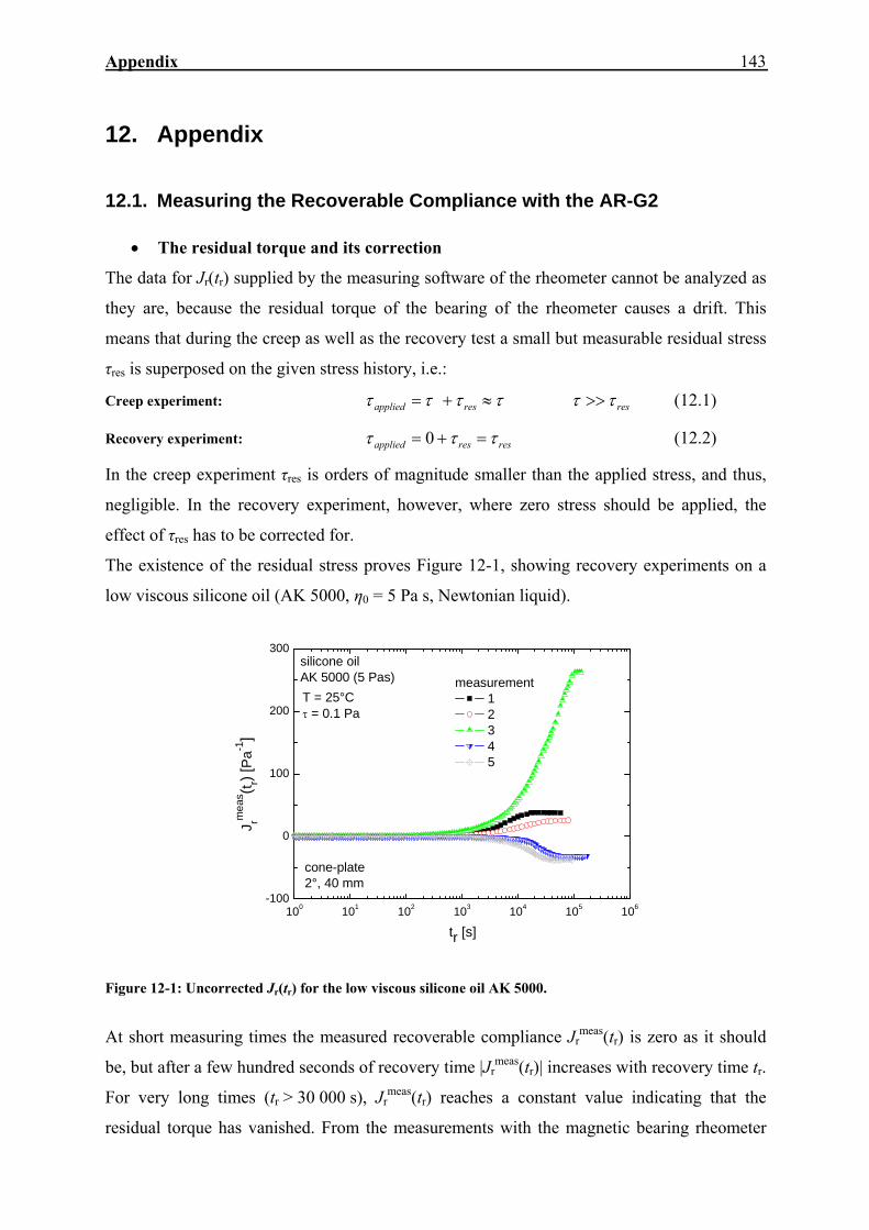
Appendix
143
12. Appendix
12.1. Measuring the Recoverable Compliance with the AR-G2
• The residual torque and its correction
The data for Jr(tr) supplied by the measuring software of the rheometer cannot be analyzed as
they are, because the residual torque of the bearing of the rheometer causes a drift. This
means that during the creep as well as the recovery test a small but measurable residual stress
τres is superposed on the given stress history, i.e.:
Creep experiment: ττττ ≈+= resapplied resττ >> (12.1)
Recovery experiment: resresapplied τττ =+= 0 (12.2)
In the creep experiment τres is orders of magnitude smaller than the applied stress, and thus,
negligible. In the recovery experiment, however, where zero stress should be applied, the
effect of τres has to be corrected for.
The existence of the residual stress proves Figure 12-1, showing recovery experiments on a
low viscous silicone oil (AK 5000, η0 = 5 Pa s, Newtonian liquid).
100 101 102 103 104 105 106-100
0
100
200
300
cone-plate2°, 40 mm
measurement 1 2 3 4 5
Jrm
eas (t r)
[Pa-1
]
tr [s]
silicone oilAK 5000 (5 Pas)T = 25°Cτ = 0.1 Pa
Figure 12-1: Uncorrected Jr(tr) for the low viscous silicone oil AK 5000.
At short measuring times the measured recoverable compliance Jrmeas(tr) is zero as it should
be, but after a few hundred seconds of recovery time |Jrmeas(tr)| increases with recovery time tr.
For very long times (tr > 30 000 s), Jrmeas(tr) reaches a constant value indicating that the
residual torque has vanished. From the measurements with the magnetic bearing rheometer
144 Appendix
MBR (Link and Schwarzl, 1985) it is well known that a point of vanishing residual torque
exists. The measurements in Figure 12-1 prove that for the AR-G2 at least two points of
vanishing residual torque are found, as can be seen from the different positive and negative
terminal values of Jrmeas(tr). In order to minimize the effects of residual torque, measurements
should be performed in the vicinity of the point(s) of vanishing residual torque. This
technique can be only applied if the characteristic point of the magnetic bearing is well
known as it is the case for the MBR. For the AR-G2, however, these points cannot be fixed
due to the missing possibility to mark them by a mapping procedure of the bearing and to
position the rotor at a certain point.
Another consequence from the experiments displayed in Figure 12-1 is that the residual
torque is not a constant for any angular position of the bearing but will vary depending on the
rotor position. Therefore, the residual torque may be a function of angular position, and thus,
a function of recovery time.
As polymer melts are much higher in viscosity than the silicone oils, the points of vanishing
residual stresses will normally be not reached during the recovery measurements. As the
recoverable deformation is typically small, and therefore, the changes in angular position will
be small, too, the assumption of a constant residual stress will be valid in most cases.
Let us assume the additivity of deformation,
)()()( rrescr
truerr
measr ttt γγγ += (12.3)
where γrmeas is the experimentally determined deformation, γr
true the unknown (true)
recoverable deformation, and γcres the additive deformation due to the superposed creep
experiment under the residual stress τres.
For the additional deformation γcres the following equation
))(()()(0
0 ηψττγ rrresrresr
resc
ttJtJt ++== (12.4)
holds with J0 being the instantaneous elastic compliance, ψ(tr) the retarded elastic compliance,
and η0 the zero shear-rate viscosity, respectively. From Equation (12.4) it is clear that for long
recovery times γcres(tr) is dominated by the flow term τres·tr/η0. Combining Equations (12.3)
and (12.4) yields
))(()()(0
0 ηψτγγ rrresr
truerr
measr
ttJtt +++= (12.5)
For its derivative with respect to the recovery time tr consequently follows
)1)(()()(0η
ψτγγ++=
r
rres
r
rtruer
r
rmeasr
dttd
dtt
dttd
(12.6)

Appendix
145
In the limit of long recovery times tr → ∞ we finally find:
0
1)(lim ητγ⋅=
∞→ resr
rmeasr
t dttd
r
(12.7)
As Jrmeas(tr) is the quantity analysed in a recovery experiment the creep stress τ has to be
introduced to Equation (12.7)
0
1)(lim ηττ ⋅=
∞→res
r
rmeasr
t dttdJ
r
(12.8)
Thus, the residual stress can be determined from the slope of the measured recoverable
compliance at recovery times longer than the longest retardation time.
r
rmeasr
res dttdJ )(
0 ⋅⋅= ηττ for ∞→t (12.9)
As a consequence of Equation (12.8), it is expected if τres ≈ const. holds that at long recovery
times the measured recoverable compliance Jrmeas(tr) should increase or decrease linearly with
recovery time depending on the sign of the residual torque (see Figure 12-2). The recoverable
compliance is then calculated from the measured data according to Equation (12.5) assuming
that tr/η0 >> J0 + ψ(tr):
rr
rmeasr
rmeasrr
truer t
dttdJtJtJ ⋅−=
)()()( (12.10)
For LCB-mLLDPE 3 at 150°C, it is shown in Figure 12-2 that a correction of the measured
recoverable compliance according to Equation (12.10) gives the same Jr(tr) and the same
constant value of Je0 in both cases.
0 6000 12000 180000.0002
0.0003
0.0004
0.0005
Jrtrue(tr)
Jrmeas(tr)
Jrtrue(tr)
Jrmeas(tr)
measurement uncorrected corrected
1
2
linear fit to determine slope
T = 150°Cτ = 30 PaJ0
e = 4.5⋅10-4 Pa-1
J r(tr)
[Pa-1
]
tr [s]
LCB-mLLDPE 3
Figure 12-2: Examples of the drift and its correction for LCB-mLLDPE 3.
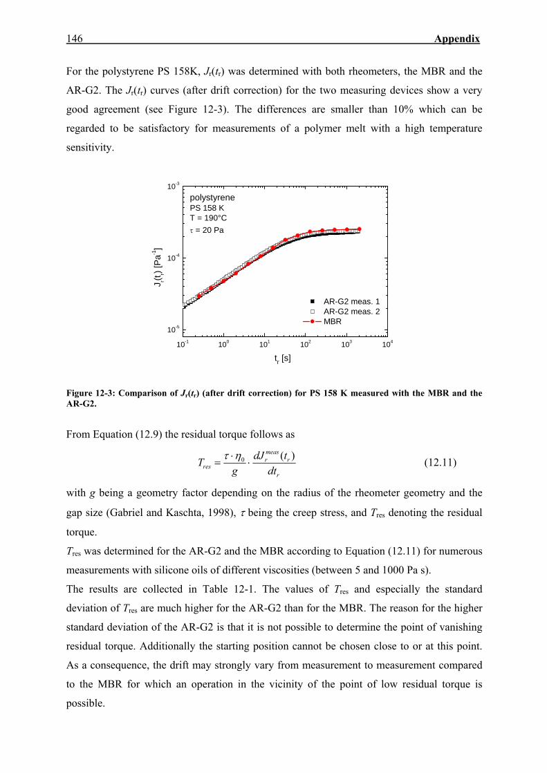
146 Appendix
For the polystyrene PS 158K, Jr(tr) was determined with both rheometers, the MBR and the
AR-G2. The Jr(tr) curves (after drift correction) for the two measuring devices show a very
good agreement (see Figure 12-3). The differences are smaller than 10% which can be
regarded to be satisfactory for measurements of a polymer melt with a high temperature
sensitivity.
10-1 100 101 102 103 104
10-5
10-4
10-3
AR-G2 meas. 1 AR-G2 meas. 2 MBR
Jr(t r) [
Pa-1]
tr [s]
polystyrenePS 158 KT = 190°Cτ = 20 Pa
Figure 12-3: Comparison of Jr(tr) (after drift correction) for PS 158 K measured with the MBR and the AR-G2.
From Equation (12.9) the residual torque follows as
r
rmeasr
res dttdJ
gT )(0 ⋅
⋅=
ητ (12.11)
with g being a geometry factor depending on the radius of the rheometer geometry and the
gap size (Gabriel and Kaschta, 1998), τ being the creep stress, and Tres denoting the residual
torque.
Tres was determined for the AR-G2 and the MBR according to Equation (12.11) for numerous
measurements with silicone oils of different viscosities (between 5 and 1000 Pa s).
The results are collected in Table 12-1. The values of Tres and especially the standard
deviation of Tres are much higher for the AR-G2 than for the MBR. The reason for the higher
standard deviation of the AR-G2 is that it is not possible to determine the point of vanishing
residual torque. Additionally the starting position cannot be chosen close to or at this point.
As a consequence, the drift may strongly vary from measurement to measurement compared
to the MBR for which an operation in the vicinity of the point of low residual torque is
possible.
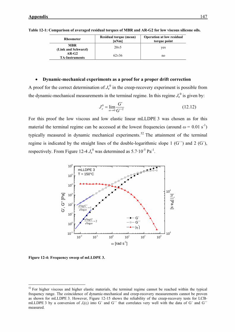
Appendix
147
Table 12-1: Comparison of averaged residual torques of MBR and AR-G2 for low viscous silicone oils.
Rheometer Residual torque (mean) [nNm]
Operation at low residual torque point
MBR (Link and Schwarzl) 20±5 yes
AR-G2 TA-Instruments 62±36 no
• Dynamic-mechanical experiments as a proof for a proper drift correction
A proof for the correct determination of Je0 in the creep-recovery experiment is possible from
the dynamic-mechanical measurements in the terminal regime. In this regime Je0 is given by:
20
0
´´´lim
GGJe →
=ω
(12.12)
For this proof the low viscous and low elastic linear mLLDPE 3 was chosen as for this
material the terminal regime can be accessed at the lowest frequencies (around ω = 0.01 s-1)
typically measured in dynamic mechanical experiments.52 The attainment of the terminal
regime is indicated by the straight lines of the double-logarithmic slope 1 (G´´) and 2 (G´),
respectively. From Figure 12-4 Je0 was determined as 5.7·10-5 Pa-1.
10-2 10-1 100 101 102 10310-1
100
101
102
103
104
105
106
G´ G´´ |η*|
ω [rad s-1]
G',
G''
[Pa]
mLLDPE 3T = 150°C
103
104
2
log´log
=ωdGd
1
log´´log
=ωdGd
|η*| [Pa s]
Figure 12-4: Frequency sweep of mLLDPE 3.
52 For higher viscous and higher elastic materials, the terminal regime cannot be reached within the typical frequency range. The coincidence of dynamic-mechanical and creep-recovery measurements cannot be proven as shown for mLLDPE 3. However, Figure 12-15 shows the reliability of the creep-recovery tests for LCB-mLLDPE 3 by a conversion of Jr(tr) into G´ and G´´ that correlates very well with the data of G´ and G´´ measured.

148 Appendix
From Figure 12-4 it can be concluded that stationarity should be reached at recovery times of
about 100 s for this material at 150°C. This information allows to estimate after which
recovery time Jr(tr) should be constant, as angular frequency ω and time t are related by
ω = 1/t. Therefore, the drift correction has to be applied at recovery times which are slightly
larger than the estimate for stationarity. A drift correction derived for a recovery time window
located at much longer times than necessary may yield wrong values for Jr(tr) if the residual
torque is not a constant but changes with angular position.
An example is given in Figure 12-5 which shows the measured and corrected recoverable
compliances of three measurements for mLLDPE 3 at T = 150°C. Experiment 1 approaches a
constant value with some experimental scatter indicating that this test was performed
accidentally in the vicinity of a point of vanishing torque. Experiment 2 coincides after the
drift correction within experimental accuracy with experiment 1. The third experiment shows
for the measured Jrmeas(tr) two approximately linear regimes of different slopes indicating a
change in the residual torque. Only the correction derived from the first linear section, which
coincides with the time range of the longest retardation time, yields data similar to the other
two measurements. For longer times the correction is too large. Therefore, those data points
will be truncated. Regarding the accuracy of the measurement, all corrected curves and the
not corrected curve of measurement 1 result in values of Je0 between 5.7·10-5 and 5.8·10-5 Pa-1.
These values are in good agreement with Je0 determined from the frequency sweep.
100 200 300 400 500
4.0x10⁻⁵
5.0x10⁻⁵
6.0x10⁻⁵
measurement uncorrected corrected 123
J r(t r) [Pa
-1]
tr [s]
mLLDPE 3T = 150 °Cτ =10 Pa
no correctionnecessary
Figure 12-5: Drift correction of Jr(tr) for mLLDPE 3 and determination of Je
0 on an extended linear scale.

Appendix
149
For materials with very long terminal retardation times (high viscosities and elasticities), e.g.,
LDPE, the terminal regime cannot be reached in dynamic-mechanical experiments because of
the very long measuring times necessary and the limited thermal stability of the materials.
Assuming that the terminal regime would be reached at ω = 0.001 s-1 and three oscillation
periods would be necessary to ensure steady-state conditions the measuring time for this
single frequency is about 18 850 s. In creep-recovery, however, the terminal regime is
reached in a creep experiment of 1000 s duration followed by a recovery test over 2000 s.
Thus, it is sufficient to determine the contribution of the long retardation times with a
measuring time of 3000 s in total.
Using the measuring time of about 18 000 s necessary for the one point dynamical experiment
at ω = 0.001 s-1 a creep-recovery experiment of that time scale (6000 s creep / 12 000 s
recovery) will provide access to dynamic moduli in a frequency range between ω = 1 s-1 and
8.3·10-5 s-1.
12.2. SEC-MALLS
The molar mass distributions of the tubular LDPE-tub 1 and LDPE-tub 4 are broader than
those of their autoclave counterparts LDPE-aut 1 and LDPE-aut 2. When plotting the raw
data from the light scattering detector using the Raleigh-ratio of the 90°-detector as a function
of elution volume, as an example, as shown in Figure 12-6 fundamental differences between
the tubular and autoclave LDPE become visible. LDPE-aut 1 and LDPE-aut 2 exhibit a peak
with a shoulder at small elution volumes. For the tubular materials, however, a bimodal peak
is observed. Therefore, the plot of the Raleigh-ratio of the 90°-detector as a function of
elution volume makes the distinctions between tubular and autoclave resins possible. Tackx
and Tacx (1998) observed similar differences between tubular and autoclave LDPE.
The Raleigh ratio is a quantity which is proportional to the product of concentration and
molar mass. The calculation of the molar mass distributions shown in Figure 6-3 is mainly
based on the concentration signal. If there are differences in the molar mass distribution, they
must be caused by differences in concentration signal and should, thus, be visible in the plot
of concentration signal as a function of elution volume, too. Figure 12-7 proofs that at elution
volumes of around 30 ml the concentration signal of LDPE-tub 1 and LDPE-aut 1 and LDPE-
tub 4 and LDPE-aut 2, respectively, is nearly the same. At these elution volumes, however,
differences in the Raleigh ratio occur, and therefore, the presence of a high or low molecular
weight tail for LDPE-tub 1 and LDPE-tub 4 can be confirmed.
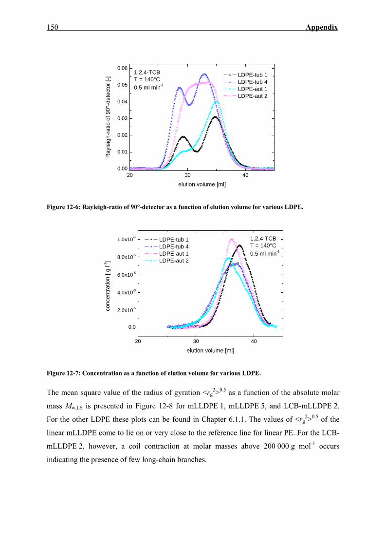
150 Appendix
20 30 400.00
0.01
0.02
0.03
0.04
0.05
0.061,2,4-TCBT = 140°C0.5 ml min-1
Ray
leig
h-ra
tio o
f 90°
-det
ecto
r [-]
elution volume [ml]
LDPE-tub 1 LDPE-tub 4 LDPE-aut 1 LDPE-aut 2
Figure 12-6: Rayleigh-ratio of 90°-detector as a function of elution volume for various LDPE.
20 30 40
0.0
2.0x10⁻⁵
4.0x10⁻⁵
6.0x10⁻⁵
8.0x10⁻⁵
1.0x10⁻⁴ 1,2,4-TCBT = 140°C0.5 ml min-1
conc
entra
tion
[ g l-1
]
elution volume [ml]
LDPE-tub 1 LDPE-tub 4 LDPE-aut 1 LDPE-aut 2
Figure 12-7: Concentration as a function of elution volume for various LDPE.
The mean square value of the radius of gyration <rg2>0.5 as a function of the absolute molar
mass Mw,LS is presented in Figure 12-8 for mLLDPE 1, mLLDPE 5, and LCB-mLLDPE 2.
For the other LDPE these plots can be found in Chapter 6.1.1. The values of <rg2>0.5 of the
linear mLLDPE come to lie on or very close to the reference line for linear PE. For the LCB-
mLLDPE 2, however, a coil contraction at molar masses above 200 000 g mol-1 occurs
indicating the presence of few long-chain branches.

Appendix
151
104 105 106
20
40
60
80
1,2,4-TCBT = 140°C
0.5 ml min-1
mLLDPE 1 mLLDPE 5 LCB-mLLDPE 2
<r2 g>0.
5 [nm
]
Mw, LS [g mol-1]
linear PE
Figure 12-8: Mean square value of the radius of gyration <rg
2>0.5 as a function of the absolute molar mass Mw,LS for mLLDPE 1, mLLDPE 5, and LCB-mLLDPE 2.
12.3. δ(|G*|)-Plots of mLLDPE 3 and mLLDPE 4
For the presumably linear material mLLDPE 3 in Figure 12-9, the δ(|G*|)-plots at four
temperatures are given. In the range of |G*| from 1000 to 10 000 Pa on the one hand a
deviation from the linear reference is observed for all temperatures, on the other hand in this
range the curves for the several temperatures split up systematically as shown in the
magnification. These findings support the thermorheologically complex behaviour found in
the temperature dependence of Je0 either caused by a small content of long-chain branching or
by an inhomogeneous comonomer distribution.
Although for mLLDPE 4 a temperature dependence of Je0 is observed, too, this material does
not show deviations in the δ(|G*|)-plots as presented in Figure 12-10.
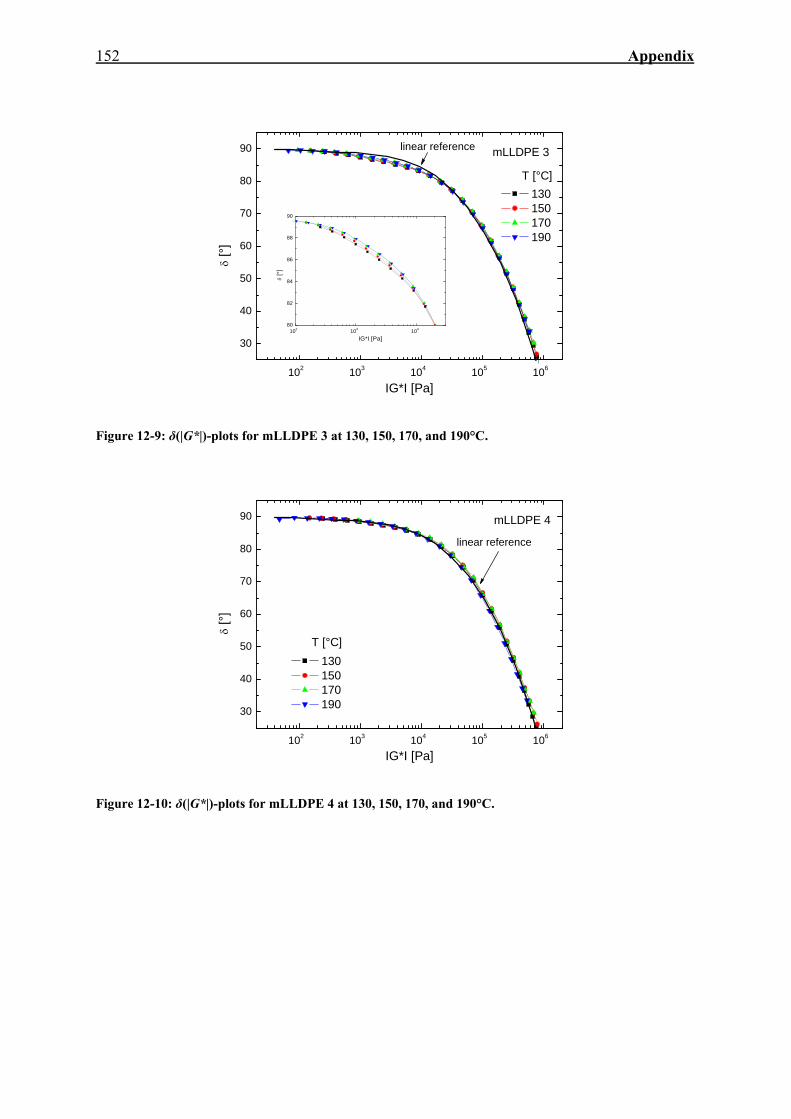
152 Appendix
102 103 104 105 106
30
40
50
60
70
80
90
102 103 10480
82
84
86
88
90
δ [°
]
IG*I [Pa]
130 150 170 190
mLLDPE 3
δ [°
]
IG*I [Pa]
T [°C]
linear reference
Figure 12-9: δ(|G*|)-plots for mLLDPE 3 at 130, 150, 170, and 190°C.
102 103 104 105 106
30
40
50
60
70
80
90
linear reference
T [°C] 130 150 170 190
δ [°
]
IG*I [Pa]
mLLDPE 4
Figure 12-10: δ(|G*|)-plots for mLLDPE 4 at 130, 150, 170, and 190°C.

Appendix
153
12.4. Mastercurves of J(t) and Jr(tr) in the Linear and Nonlinear Regime
• Thermorheologically simple material (linear PP)
J(t) and Jr(tr) for the material PP 10 measured at three different temperatures are shifted to a
reference temperature of 180°C using the activation energy determined from the zero shear-
rate viscosities. This is shown in Figure 12-11 and Figure 12-12 for shear stresses in the linear
regime at 10 Pa and in the nonlinear regime at 1000 Pa, respectively. As expected from the
time-temperature-superposition principle, the construction of a master curve is possible as
well for J(t) as for Jr(tr) using the same shift factors in the linear and nonlinear stress regime.
This is a proof for the thermorheological simplicity of the linear PP.
Regarding Jr(tr) a change in temperature only causes a time-dependent shift of the curve,
whereas, the stationary values Je and Je0, respectively, are the same independent of
temperature. These findings are in accordance to the literature (Münstedt, 1975, Meissner,
1975, Wagner and Laun, 1978, Orbon and Plazek, 1979, Münstedt and Laun, 1979, Laun,
1987, Gabriel et al., 1998, Gabriel and Münstedt, 1999).
0.1 1 10 100 1000 1000010-5
10-4
10-3
10-2
10-1
180°C 200°C 220°C
J(t/a
T), J r(t 0/a
T,t r/aT) [
Pa-1
]
t/aT, tr/aT [s]
PP 10τ = 10 PaT0 = 180°CEa = 40.9 kJ/mol
T
Figure 12-11: Mastercurves of J(t) and Jr(tr) for PP 10 in the linear stress regime at a reference temperature T0 = 180°C (Wolff, 2008).
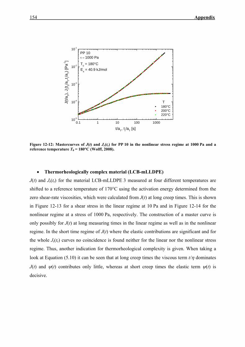
154 Appendix
0.1 1 10 100 100010-5
10-4
10-3
10-2
10-1
180°C 200°C 220°C
T
T0 = 180°CEa = 40.9 kJ/mol
J(t/a
T), J r(t 0/a
T,t r/aT) [
Pa-1
]
t/aT, tr/aT [s]
PP 10τ = 1000 Pa
Figure 12-12: Mastercurves of J(t) and Jr(tr) for PP 10 in the nonlinear stress regime at 1000 Pa and a reference temperature T0 = 180°C (Wolff, 2008).
• Thermorheologically complex material (LCB-mLLDPE)
J(t) and Jr(tr) for the material LCB-mLLDPE 3 measured at four different temperatures are
shifted to a reference temperature of 170°C using the activation energy determined from the
zero shear-rate viscosities, which were calculated from J(t) at long creep times. This is shown
in Figure 12-13 for a shear stress in the linear regime at 10 Pa and in Figure 12-14 for the
nonlinear regime at a stress of 1000 Pa, respectively. The construction of a master curve is
only possibly for J(t) at long measuring times in the linear regime as well as in the nonlinear
regime. In the short time regime of J(t) where the elastic contributions are significant and for
the whole Jr(tr) curves no coincidence is found neither for the linear nor the nonlinear stress
regime. Thus, another indication for thermorheological complexity is given. When taking a
look at Equation (5.10) it can be seen that at long creep times the viscous term t/η dominates
J(t) and ψ(t) contributes only little, whereas at short creep times the elastic term ψ(t) is
decisive.

Appendix
155
10-1 100 101 102 103 10410-5
10-4
10-3
10-2
10-1
100
J
J(t/a
T), J
r(t0/
a T,t r/aT)
[Pa-1
]
t/aT, tr/aT [s]
130°C 150°C 170°C 190°C
Jr T
LCB-mLLDPE 3τ = 10 PaT0 = 170°CEa = 48.9 kJ/mol
Figure 12-13: Mastercurves of J(t) and Jr(tr) for LCB-mLLDPE 3 in the linear stress regime at a reference temperature T0 = 170°C.
10-1 100 101 102 103 10410-5
10-4
10-3
10-2
10-1
LCB-mLLDPE 3τ = 1000 PaT0 = 170°CEa = 48.9 kJ/mol
J
J(t/a
T), J
r(t0/
a T,t r/aT)
[Pa-1
]
t, tr [s]
130°C 150°C 170°C 190°C
Jr T
Figure 12-14: Mastercurves of J(t) and Jr(tr) for LCB-mLLDPE 3 in the nonlinear stress regime at 1000 Pa at a reference temperature T0 = 170°C.
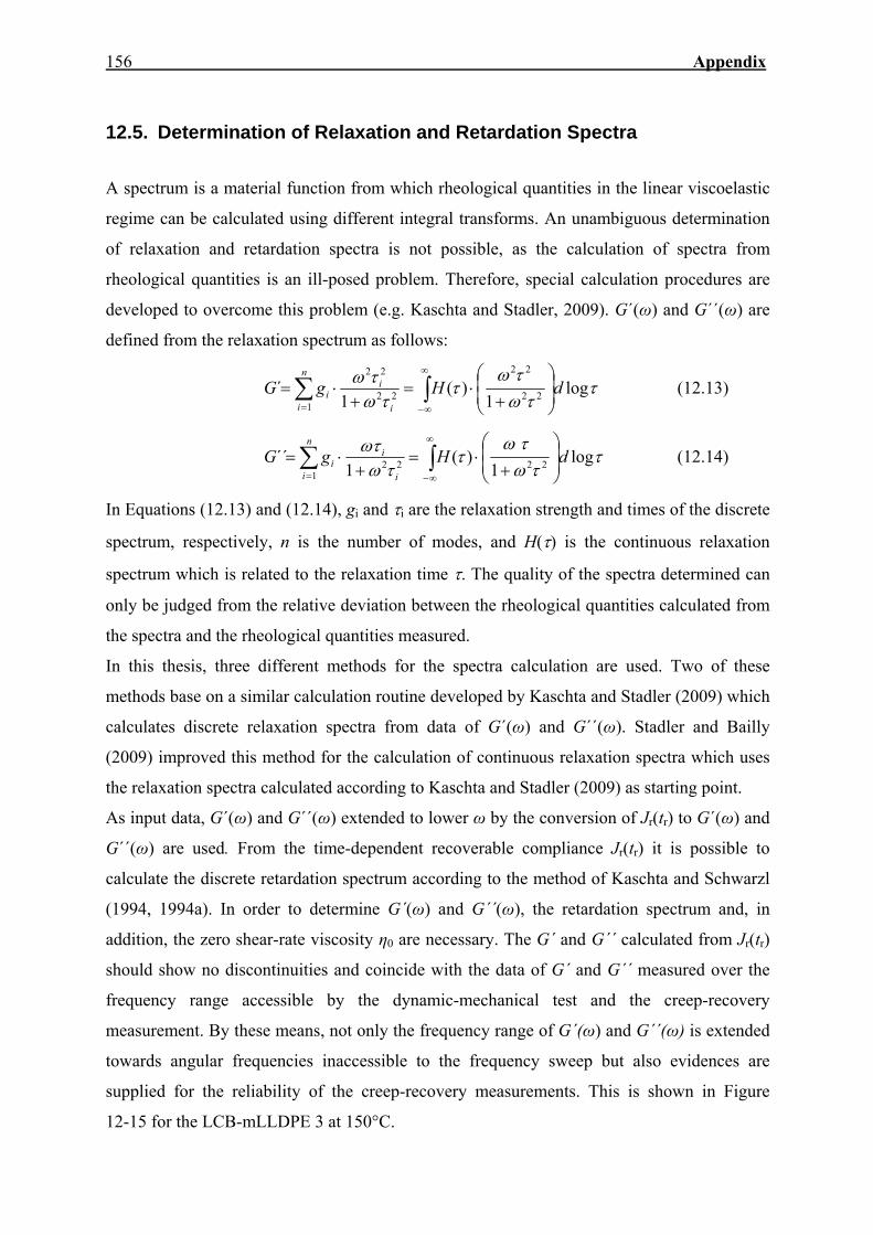
156 Appendix
12.5. Determination of Relaxation and Retardation Spectra
A spectrum is a material function from which rheological quantities in the linear viscoelastic
regime can be calculated using different integral transforms. An unambiguous determination
of relaxation and retardation spectra is not possible, as the calculation of spectra from
rheological quantities is an ill-posed problem. Therefore, special calculation procedures are
developed to overcome this problem (e.g. Kaschta and Stadler, 2009). G´(ω) and G´´(ω) are
defined from the relaxation spectrum as follows:
ττω
τωτ
τωτω log
1)(
1´ 22
22
22
22
1dHgG
i
in
ii ⎟
⎟⎠
⎞⎜⎜⎝
⎛
+⋅=
+⋅= ∫∑
∞
∞−=
(12.13)
ττω
τωτ
τωωτ log
1)(
1´´ 2222
1dHgG
i
in
ii ⎟
⎟⎠
⎞⎜⎜⎝
⎛
+⋅=
+⋅= ∫∑
∞
∞−=
(12.14)
In Equations (12.13) and (12.14), gi and τi are the relaxation strength and times of the discrete
spectrum, respectively, n is the number of modes, and H(τ) is the continuous relaxation
spectrum which is related to the relaxation time τ. The quality of the spectra determined can
only be judged from the relative deviation between the rheological quantities calculated from
the spectra and the rheological quantities measured.
In this thesis, three different methods for the spectra calculation are used. Two of these
methods base on a similar calculation routine developed by Kaschta and Stadler (2009) which
calculates discrete relaxation spectra from data of G´(ω) and G´´(ω). Stadler and Bailly
(2009) improved this method for the calculation of continuous relaxation spectra which uses
the relaxation spectra calculated according to Kaschta and Stadler (2009) as starting point.
As input data, G´(ω) and G´´(ω) extended to lower ω by the conversion of Jr(tr) to G´(ω) and
G´´(ω) are used. From the time-dependent recoverable compliance Jr(tr) it is possible to
calculate the discrete retardation spectrum according to the method of Kaschta and Schwarzl
(1994, 1994a). In order to determine G´(ω) and G´´(ω), the retardation spectrum and, in
addition, the zero shear-rate viscosity η0 are necessary. The G´ and G´´ calculated from Jr(tr)
should show no discontinuities and coincide with the data of G´ and G´´ measured over the
frequency range accessible by the dynamic-mechanical test and the creep-recovery
measurement. By these means, not only the frequency range of G´(ω) and G´´(ω) is extended
towards angular frequencies inaccessible to the frequency sweep but also evidences are
supplied for the reliability of the creep-recovery measurements. This is shown in Figure
12-15 for the LCB-mLLDPE 3 at 150°C.

Appendix
157
10-4 10-3 10-2 10-1 100 101 102 103 10410-2
10-1
100
101
102
103
104
105
106
G´ G´´ G´ calculated from Jr(tr) G´´ calculated from Jr(tr)
ω [rad s-1]
G',
G'' [
Pa]
LCB-mLLDPE 3T = 150 °C
lowest frequencytypically chosen
Figure 12-15: G´(ω) and G´´(ω) measured and calculated from Jr(tr) for LCB-mLLDPE 3.
Schwarzl developed the third method for the calculation of relaxation spectra presented in this
thesis. In the first step the storage and loss compliance J´(ω) and J´´(ω) are calculated from
the experimental data of J(t) and Jr(tr) by using approximations published by Schwarzl (1970).
J´(ω) and J´´(ω) can be converted into G´(ω) and G´´(ω) using the following equations:
22 )´´()´()´()´(
ωωωωJJ
JG+
= (12.15)
22 )´´()´()´´()´´(
ωωωωJJ
JG+
= (12.16)
By these means also an extended data set for G´(ω) and G´´(ω) is obtained. From this data set
the relaxation spectrum is calculated by setting fixed relaxation times τi with a logarithmical
spacing of 10/1 =+ ii ττ and by varying the relaxation strength until the deviation between
the measured moduli Gi´m and Gi´´m and the calculated moduli Gi´c and Gi´´c corresponding to
the variance V is minimized (Schwarzl, 2008).
∑= ⎪⎭
⎪⎬⎫
⎪⎩
⎪⎨⎧
⎟⎟⎠
⎞⎜⎜⎝
⎛ −+⎟⎟
⎠
⎞⎜⎜⎝
⎛ −−
=n
imi
mi
ci
mi
mi
ci
GGG
GGG
nV
1
22
´´´´´´
´´´
121
(12.17)
In some cases, better results are obtained if the spectrum is determined in three steps. In a first
step, a spectrum is determined with relaxation times τi of a logarithmical spacing of 10. In the
next step, a second spectrum is calculated by the same method, however, by setting different
fixed relaxation times τi that are shifted by a factor of 10 compared to the relaxation times
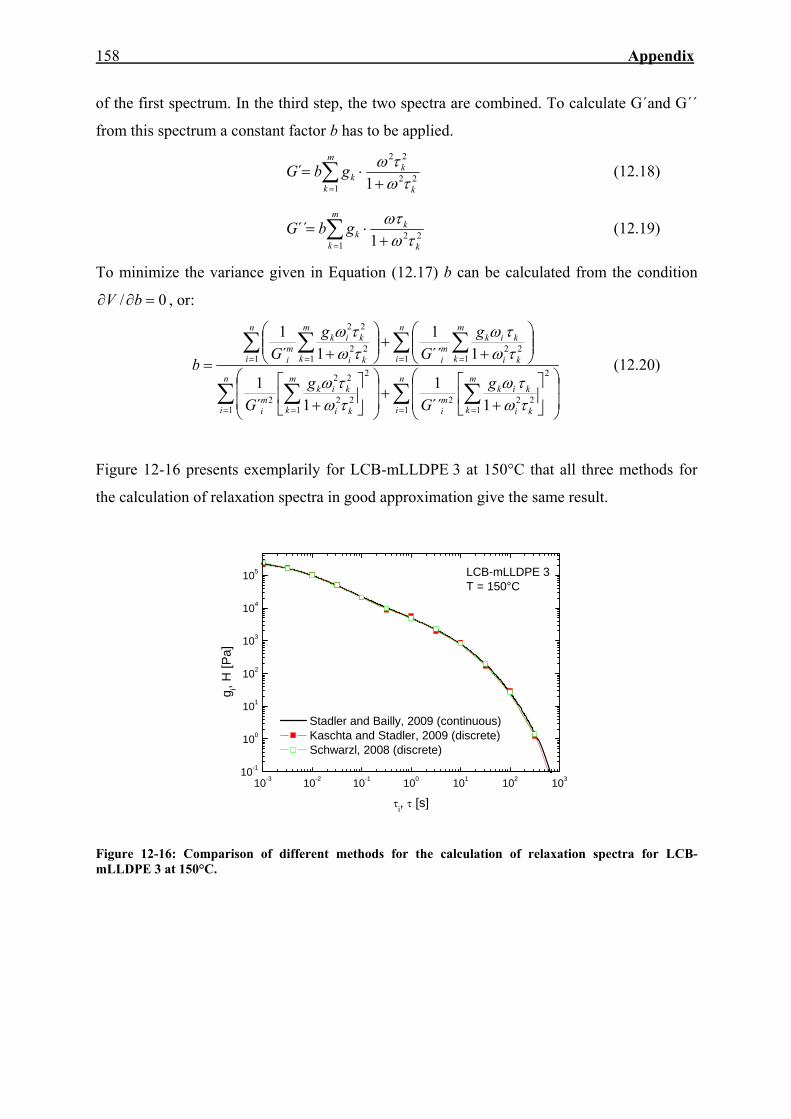
158 Appendix
of the first spectrum. In the third step, the two spectra are combined. To calculate G´and G´´
from this spectrum a constant factor b has to be applied.
22
22
1 1´
k
km
kkgbG
τωτω
+⋅= ∑
=
(12.18)
221 1
´´k
km
kkgbG
τωωτ+
⋅= ∑=
(12.19)
To minimize the variance given in Equation (12.17) b can be calculated from the condition
0/ =∂∂ bV , or:
∑ ∑ ∑∑
∑ ∑ ∑∑
= = ==
= = ==
⎟⎟
⎠
⎞
⎜⎜
⎝
⎛⎥⎦
⎤⎢⎣
⎡+
+⎟⎟
⎠
⎞
⎜⎜
⎝
⎛⎥⎦
⎤⎢⎣
⎡+
⎟⎟⎠
⎞⎜⎜⎝
⎛+
+⎟⎟⎠
⎞⎜⎜⎝
⎛+
=n
i
n
i
m
k ki
kikmi
m
k ki
kikmi
n
i
n
i
m
k ki
kikmi
m
k ki
kikmi
gG
gG
gG
gG
b
1 1
2
1222
2
122
22
2
1 1 122
122
22
1´´1
1´1
1´´1
1´1
τωτω
τωτω
τωτω
τωτω
(12.20)
Figure 12-16 presents exemplarily for LCB-mLLDPE 3 at 150°C that all three methods for
the calculation of relaxation spectra in good approximation give the same result.
10-3 10-2 10-1 100 101 102 10310-1
100
101
102
103
104
105
g i, H [P
a]
τi, τ [s]
Stadler and Bailly, 2009 (continuous) Kaschta and Stadler, 2009 (discrete) Schwarzl, 2008 (discrete)
LCB-mLLDPE 3T = 150°C
Figure 12-16: Comparison of different methods for the calculation of relaxation spectra for LCB-mLLDPE 3 at 150°C.

Appendix
159
• Contribution of relaxation times τi to η0 and Je0
For the interpretation of the stress dependence of η and Je it is assumed in Chapter 7.2.6 that
η0 is determined by the product of relaxation strength and relaxation time (see Equation (7.6)).
For Je0, however, the longer relaxation times are decisive because the contribution of the
relaxation strength is approximately proportional to the square of the relaxation time. This is
not obvious at the first glance from Equation (7.7). Therefore, in Figure 12-17 the
contributions of the different relaxation times τi to η and Jr according to Equations (7.6) and
(7.7) are shown for the relaxation spectrum of LCB-mLLDPE 3 at 150°C.53 For a better
presentation the cumulative curves are normalized by η0 and Je0, respectively. As expected,
there is a shift between the cumulative curve of η and Jr of 1 to 2 orders of magnitude in
relaxation time. The cumulative curve for η starts to increase at shorter relaxation times and
reaches a plateau value at long relaxation times. The cumulative curve for Jr increases much
slowlier at the short relaxation times, increases steeper at the longer relaxation times and
reaches a plateau value at longer relaxation times than the curve for η.
10-3 10-2 10-1 100 101 102 103 1040.0
0.5
1.0
η(τ i)/η
0 ,J
r(τi)/J
0 e
τi [s]
η(τi)/η0
Jr(τi)/J0e
LCB-mLLDPE 3T = 150°C
Figure 12-17: Contribution of relaxation times τi to η and Jr normalized by η0 and Je
0.
53 The calculation of the contributions of the different relaxation times to η and Jr was performed by Prof. Dr. Stadler (Stadler, 2009).
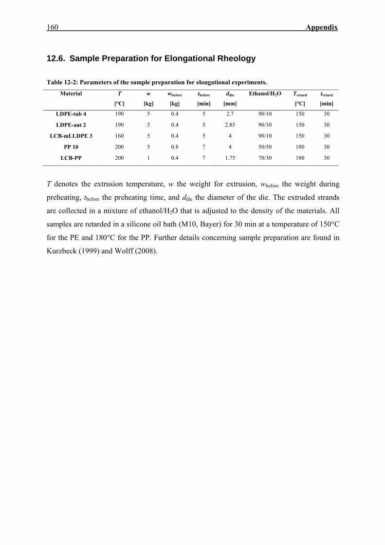
160 Appendix
12.6. Sample Preparation for Elongational Rheology Table 12-2: Parameters of the sample preparation for elongational experiments.
Material T
[°C]
w
[kg]
wbefore
[kg]
tbefore
[min]
ddie
[mm]
Ethanol/H2O Tretard
[°C]
tretard
[min]
LDPE-tub 4 190 5 0.4 5 2.7 90/10 150 30
LDPE-aut 2 190 5 0.4 5 2.85 90/10 150 30
LCB-mLLDPE 3 160 5 0.4 5 4 90/10 150 30
PP 10 200 5 0.8 7 4 50/50 180 30
LCB-PP 200 1 0.4 7 1.75 70/30 180 30
T denotes the extrusion temperature, w the weight for extrusion, wbefore the weight during
preheating, tbefore the preheating time, and ddie the diameter of the die. The extruded strands
are collected in a mixture of ethanol/H2O that is adjusted to the density of the materials. All
samples are retarded in a silicone oil bath (M10, Bayer) for 30 min at a temperature of 150°C
for the PE and 180°C for the PP. Further details concerning sample preparation are found in
Kurzbeck (1999) and Wolff (2008).

Appendix
161
12.7. Zero Shear-Rate Viscosities at Different Temperatures
In Table 12-3, the values of the zero shear-rate viscosities η0 of various PE and PP measured
at different temperatures are collected. For some of the PP η0 was only determined at 180°C.
The values of η0 at 180°C for these materials are not listed here but can be found in Table 6-2.
Table 12-3: Zero shear-rate viscosities η0 of PE and PP at various measuring temperatures.*
Material η0 at 130°C [Pa s] η0 at 150°C [Pa s] η0 at 170°C [Pa s] η0 at 190°C [Pa s]
linear mLLDPE
mLLPDE 1 n.d.** 2370±10 1580±10 1160±20
mLLPDE 2 26 130±650 15 500±640 10 270±440 7160±350
mLLPDE 3 24 860±480 15 060±80 9570±440 6320±150
mLLPDE 4 23 740±180 13 850±80 8930±50 6200±40
mLLPDE 5 25 990±67 16 420±430 10 770±31 7050±100
LCB-mLLDPE
LCB-mLLDPE 1 68 200±1820 33 100±1040 17 180±380 9830±280
LCB-mLLDPE 2 28 310±280 14 690±150 7790±30 4490±40
LCB-mLLDPE 3 88 710±1030 45 410±680 22 080±620 13 420±160
LCB-mLLDPE 4 68 880±2980 33 090±420 18 320±1070 10 880±260
LDPE tubular
LDPE-tub 1 4880±10 2060±10 1070±10 590±10
LDPE-tub 2 150 300±8000 60 700±5100 27 100±1500 12 600±400
LDPE-tub 3 930 700±26 100 347 400±14 800 148 000±2900 65050±2470
LDPE-tub 4 1 317 500±35 900 481 300±14 200 197 400±7700 92 860±4960
LDPE autoclave
LDPE-aut 1 30 850±280 13 140±480 6500±70 3400±90
LDPE-aut 2 688 000±15 900 277 800±5600 115 200±800 51 900±2100
η0 at 180°C [Pa s] η0 at 200°C [Pa s] η0 at 220°C [Pa s]
linear PP***
PP 3 3340±10 1990±40 1320±60
PP 7 7650±250 4880±100 3130±45
PP 10 48 690±960 30 140±910 20 190±570
PP 11 168 000±20100 108 000±4700 n.d.
* The values of η0 in this table are average values from at least four individual measurements. ** Because of the high melting temperature Tm η0 at 130°C could not be determined. *** For the PP not listed, η0 was only determined at 180°C (see Table 6-2).

162 Appendix
12.8. Temperature Rising Elution Fractionation (TREF)
The material PP 7 shows a higher Je0 as well as a higher S0 than could be expected from SEC-
MALLS characterization. IR-spectroscopy and DSC analysis do not show any evidence of a
possible comonomer content or atacticity. Therefore, on this material and on a reference
material (PP 3) a TREF analysis was conducted at the laboratory of Polymer Char S.A..
TREF is a technique for the fractionation of semi-crystalline polymers according to the
degree of crystallinity. For PP, the ability of a molecule to crystallize is determined by its
tacticity. The basic principle of TREF is that a material with a high level of crystallizability
crystallizes from solution at a higher temperature than a material with a lower level. In a first
step, crystalline material is prepared by slowly cooling down a dilute solution. Then the
crystalline material is packed into a column through which a solvent is passed. The
temperature of the solvent is gradually increased, and an IR-detector analyzes the
concentration of the polymer in the effluent. The results of a TREF analysis are typically
plotted as the concentration of the polymer in the effluent as a function of temperature, as
shown in Figure 12-18.
For the two PP, analyzed significant differences in the crystallization behaviour are not
visible. If higher amounts of atactic structures would be present they would lead to a broader
concentration peak.
20 40 60 80 100 120 140-2
0
2
4
6
8
10
12
14
16
18
20
conc
entra
tion
dw/d
T
T [°C]
PP 3 PP 7
Figure 12-18: TREF analysis for PP 3 and PP 7.

Appendix
163
12.9. Stress Dependence of Viscosity and Elasticity at Different Temperatures
In Chapter 7.2.4, the stress dependence of η at different temperatures and the construction of
a mastercurve are presented for one example of each material class (mLLDPE 4, LCB-
mLLDPE 3, and LDPE-tub 1). η(τ) was determined for mLLDPE 1, mLLDPE 5, and LCB-
mLLDPE 2 at various temperatures, too. The following figures Figure 12-19, Figure 12-20,
and Figure 12-21 present η(τ) at the different temperatures and the mastercurve of η(τ) at a
reference temperature of 170°C. In order to show that the calculation of a mastercurve of η(τ)
is possible for a linear PP, too, Figure 12-22 presents the procedure of the construction of a
mastercurve for PP 10.
Figure 12-19: (a) Stress dependence of the steady-state viscosity η for mLLDPE 1 at 150, 170, and 190°C. (b) Mastercurve of the steady-state viscosity η as a function of stress τ for mLLDPE 1 at a reference temperature of T0 = 170°C.
Figure 12-20: (a) Stress dependence of the steady-state viscosity η for mLLDPE 5 at 130 and 170°C. (b) Mastercurve of the steady-state viscosity η as a function of stress τ for mLLDPE 5 at a reference temperature of T0 = 170°C.
1 10 100 1000 10000
103
1.5x10³
2x10³
2.5x10³
3x10³
150°C 170°C 190°C
η [P
a s]
τ [Pa]
mLLDPE 1
(a)1 10 100 1000 10000
103
1.2x10³
1.4x10³
1.6x10³
1.8x10³
2x10³
150°C 170°C 190°C averages
η⋅a T [P
a s]
τ [Pa]
mLLDPE 1
T0 = 170°C
(b)
10 100 1000 10000
104
1.5x10⁴
2x10⁴
2.5x10⁴
3x10⁴
130°C 170°Cη
[Pa
s]
τ [Pa]
mLLDPE 5
(a)10 100 1000 10000
9x10³
104
1.1x10⁴
1.2x10⁴
T0 = 170°C
130°C 170°C averages
η⋅a T [P
a s]
τ [Pa]
mLLDPE 5
(b)

164 Appendix
Figure 12-21: (a) Stress dependence of the steady-state viscosity η for LCB-mLLDPE 2 at 130, 150, 170, and 190°C. (b) Mastercurve of the steady-state viscosity η as a function of stress τ for LCB-mLLDPE 2 at a reference temperature of T0 = 170°C.
Figure 12-22: (a) Stress dependence of the steady-state viscosity η for PP 10 at 180, 200, and 220°C. (b) Mastercurve of the steady-state viscosity η as a function of stress τ for PP 10 at a reference temperature of T0 = 200°C. The temperature-dependent Je(τ) and their mastercurves are shown in Chapter 7.2.4 for
mLLDPE 1, mLLDPE 4, LCB-mLLDPE 3, and LDPE-tub 1.54 The temperature-dependent
Je(τ) and their mastercurves for mLLDPE 5 and LCB-mLLDPE 2 are presented in Figure 12-
23 and Figure 12-24.
54 Each measuring point for η and Je in the Figures 12-19 to 12-24 is the average of at least three measurements. The error bars are caluculated as the standard deviation from these measurements. The error bars for the average measuring points from all temperatures are calculated as the average of the error bars from each temperature.
1 10 100 1000 10000
4000
5000
6000
7000
8000
T0 = 170°C
130°C 150°C 170°C 190°C averages
η⋅a T [
Pa
s]
τ [Pa]
LCB-mLLDPE 2
(b)1 10 100 1000 10000
103
104
LCB-mLLDPE 2
130°C 150°C 170°C 190°C
η [P
a s]
τ [Pa] (a)
1 10 100 1000 10000
2x10⁴
4x10⁴
6x10⁴
8x10⁴
PP 10
180°C 200°C 220°C
η [P
a s]
τ [Pa] (a)1 10 100 1000 10000
2x10⁴
2.5x10⁴
3x10⁴
3.5x10⁴
T0 = 200°C
PP 10
180°C 200°C 220°C averages
η⋅a T [P
a s]
τ [Pa] (b)

Appendix
165
For mLLDPE 5, the Je0 can be regarded as temperature-independent as the error bars overlap.
At the stresses in the nonlinear regime, however, the Je at 130°C consistently lie higher than
at 170°C in the order of magnitude expected from the density change with temperature. For
this reason a mastercurve is calculated, which is used for the comparison of the stress-
dependent Je of the PE as a function of molecular structure in Chapter 7.2.5.
Figure 12-23: (a) Stress dependence of the steady-state elastic compliance Je for mLLDPE 5 at 130 and 170°C. (b) Mastercurve of the steady-state elastic compliance Je as a function of stress τ for mLLDPE 5 at a reference temperature of T0 = 170°C.
Figure 12-24: (a) Stress dependence of the steady-state elastic compliance Je for LCB-mLLDPE 2 at 130, 150, 170, and 190°C. (b) Mastercurve of the steady-state elastic compliance Je as a function of stress τ for LCB-mLLDPE 2 at a reference temperature of T0 = 170°C.
The mastercurves for η(τ) and Je(τ) are used for the discussion of stress dependence of
viscosity and elasticity as function of molecular structure in Chapter 7.2.5. For the materials
neither presented in Chapter 7.2.4 nor here but discussed in Chapter 7.2.5, the stress
dependence of η and Je was determined at only one measuring temperature, 170°C for PE and
180°C for PP.
10 100 1000 1000010-5
2x10⁻⁵
3x10⁻⁵
4x10⁻⁵
5x10⁻⁵
6x10⁻⁵
7x10⁻⁵
130°C 170°C
J e [Pa-1
]
τ [Pa]
mLLDPE 5
(a) 10 100 1000 1000010-5
2x10⁻⁵
3x10⁻⁵
4x10⁻⁵
5x10⁻⁵
6x10⁻⁵
7x10⁻⁵
T0 = 170°C
130°C 170°C averages
J e⋅bT [P
a-1]
τ [Pa]
mLLDPE 5
(b)
1 10 100 1000 10000
10-4
2x10⁻⁴
3x10⁻⁴
4x10⁻⁴
5x10⁻⁴
6x10-47x10-4
130°C 150°C 170°C 190°C
LCB-mLLDPE 2
J e [Pa-1
]
τ [Pa] (a)1 10 100 1000 10000
10-4
2x10⁻⁴
3x10⁻⁴
4x10⁻⁴
T0 = 170°C
J e⋅bT [P
a-1]
τ [Pa]
LCB-mLLDPE 2
130°C 150°C 170°C 190°C averages
(b)

166 Appendix
12.10. Numerical description of the stress dependence of Je The Carreau-Yasuda model is a practical tool for the description of various types of viscosity
functions (Carreau, 1968, Yasuda, 1979). As the curves for the viscosity and the steady-state
elastic compliance as a function of stress have similar shapes this model is adapted to
describe Je, too.
In this way, a correlation of the stress dependence of elasticity with molecular structure,
molar mass, and molar mass distribution may be possible. For the steady-state elastic
compliance as a function of stress τ the model reads:
an
aee JJ
10 ])(1[)(
−
⋅+= τλτ (12.21)
λ in [Pa-1] describes the onset of the stress-dependent regime, a characterizes the shape of the
intermediate regime between the stress-dependent and the linear regime, and n - 1 is the
double-logarithmic slope attained at high stresses.
Figure 12-25 gives the principle of the Carreau-Yasuda-fit. If the regimes at the lowest and at
the highest stresses where the slope is constant are fitted, linearily the intersection point of
these two lines is located at 1/λ.
Figure 12-25 shows another two examples for the good quality of the fit (full lines) for the
mastercurves of LCB-mLLDPE 2 and LDPE-tub 1 at a reference temperature of 170°C.
Where available, for the PE the mastercurves of Je(τ) at 170°C are used for analysis. For the
rest of the PE the curves at 170°C and for the PP the curves at 180°C are fitted.
1 10 100 1000 10000
10-4
2x10⁻⁴
3x10⁻⁴
4x10⁻⁴
5x10⁻⁴
6x10-47x10-4
T0 = 170°C
LDPE-tub 1 LCB-mLLDPE 2 fit a ≠ 1 fit a ≠ 1 fit a = 1 fit a = 1
J e [Pa-1
]
τ [Pa]
≈ 1/λJ0
e
Figure 12-25: Principle of the Carreau-Yasuda-fit for Je(τ) and examples for fits for LCB-mLLDPE 2 and LDPE-tub 1 with a = 1 and with a ≠ 1.

Appendix
167
Parameter a in Equation (12.21) can also be set to 1 and the description of the data remains of
the same quality as is shown in Figure 12-25 (dashed line), too. For the linear PP presented in
Figure 12-26, the fits with a = 1 (dashed line) describe the data a bit better than the fits with
a ≠ 1 (full line) especially at high shear stresses. Therefore, for the correlation with Je0 and the
properties from the MMD the fit parameters λ of the fits with a = 1 are used.
10 100 1000 10000
10-4
10-3
PP 1 PP 6 PP 8 PP 9 fit a ≠ 1 fit a = 1
T = 180°C
J e [Pa-1
]
τ [Pa]
Figure 12-26: Examples for Carreau-Yasuda-fits for various PP with a = 1 and with a ≠ 1.
Figure 12-27 presents the fit parameter λ as a function of Je0 for various PE and PP. For the
PE as well as for the PP, λ increases with increasing Je0. For the PE and PP, respectively,
indepentenly of the presesence of long-chain branches an approximately linear relationship
between Je0 and λ, which marks the onset of nonlinearity, is found.
λ correlates with the onset of the nonlinear stress regime. The higher λ the lower is the onset
of the nonlinear regime. Therefore, these findings correspond to those of Chapter 7.2.5 where
an increasing stress dependence of Je with increasing Je0 was observed.

168 Appendix
10-4 10-3 10-2
10-3
10-2
λ [P
a-1]
J0e [Pa-1]
mLLDPE LCB-mLLDPE LDPE
PP LCB-PP
PE: T0 = 170°CPP: T = 180°C
Figure 12-27: Correlation of fit parameter λ (from fit with a ≠ 1) with Je
0.
12.11. Determination of Extrudate Swell
The extrudate swell S for most of the linear PP55 and the LDPE is determined as explained in
Chapter 5.2. To make a comparison between the different PP and LDPE possible it is
important to measure the equilibrium extrudate swell S0 which is obtained after retardation in
an oil bath. Therefore, for all materials the dependence of S from retardation time tretard has to
be investigated.
For PP 1, PP 8, and PP 10, this dependence is presented in Figure 12-28 at 180°C for a shear
stress τw = 17 700 Pa calculated according to Equation (5.18). For PP 10 and PP 8 having
high viscosities and elasticities, after 20 min of retardation S0 is attained, whereas for the
lower viscous and elastic PP 1 S0 is already reached after the shortest retardation of 5 min.
55 For the LCB-PP, the extrudate swell could not be determined due to the high viscosity of the material. For the PP 5, not enough material was available for the determination of S0.

Appendix
169
5 10 15 20 25 300.12
0.14
0.16
0.18
0.20
0.22
0.24
0.26
PP 1 PP 8 PP 10
S [-]
tretard [min]
T = 180°Cτw = 17 670 Pa
Figure 12-28: Extrudate swell S as a function of retardation time for PP 1, PP 8, and PP 10 at 180°C and τw = 17 700 Pa. In Table 12-4, the values for S0 determined under different measuring conditions are listed. In
Figure 12-29, a correlation between S0 and Je0 is presented.
At the conditions of T = 180°C and τw = 17 700 Pa a linear correlation is found between Je0
and S0. This seems surprising as on the one hand Je0 is a quantity determined in the linear
stress regime at stresses three orders of magnitude smaller than τw and on the other hand S0 is
a nonlinear quantity influenced by shear and elongational deformation. Nevertheless, a
qualitative correlation between these two quantities is possible. Fujiyama and Awaya (1972)
also find a linear correlation between the extrudate swell and Je0 for polypropylenes.
Table 12-4: Equilibrium extrudate swell S0 of various linear PP determined at 180°C and τw = 17 700 Pa, at 200°C and τw = 17 700 Pa, and at 180°C and τw = 44 200 Pa.
Material S0 [-] (τw = 17 700 Pa, 180°C)
S0 [-] (τw = 17 700 Pa, 200°C)
S0 [-] (τw = 44 200 Pa, 180°C)
PP 1 0.166±0.004 - -
PP 2 0.159±0.021 - -
PP 3 0.217±0.008 - -
PP 4 0.281±0.024 - -
PP 6 0.354±0.012 0.371±0.001 -
PP 7 0.329±0.015 - 0.581±0.003
PP 8 0.210±0.013 0.233±0.012 0.490±0.016
PP 9 0.178±0.005 0.170±0.007 0.375±0.007
PP 10 0.241±0.016 0.228±0.009 0.421±0.026
PP 11 - 0.239±0.002 -

170 Appendix
0.0 5.0x10⁻⁴ 1.0x10⁻³ 1.5x10⁻³
0.2
0.3
0.4
0.5
0.6
0.7
180°C, τw= 17 700 Pa 180°C, τw= 44 200 Pa 200°C, τw= 17 700 Pa
S0 [-
]
J0e [Pa-1]
PP
Figure 12-29: Correlation between equilibrium extrudate swell S0 and linear steady-state elastic compliance Je
0 for PP at 180°C and τw = 17 700 Pa, at 200°C and τw = 17 700 Pa, and at 180°C and τw = 44 200 Pa.
In order to investigate the temperature dependence of the extrudate swell for PP 6, PP 8, PP 9,
PP 10, and PP 11 S0 is determined at 200°C and τw = 17 700 Pa, too (see also Figure 12-29
and Table 12-4). Considering the accuracy of the measurement S0 proves to be independent of
temperature. Romanini and Pezzin (1982) report for linear PP with Mw between 270 and
680 kg mol-1 and Mw/Mn between 7 and 9.7 that S0 is independent of temperature in the range
of 180 to 250°C. Also Fujiyama and Inata (2002) find S0 of two Z/N-PP with
Mw = 434 kg mol-1 and Mw/Mn = 6.0 and Mw = 416 kg mol-1 and Mw/Mn = 6.2 to be
independent of temperature, however, in the range between 210°C and 270°C.
S0 of PP 7, PP 8, PP 9, and PP 10 are additionally measured at 180°C and τw = 44 200 Pa. The
results are presented in Figure 12-29 and Table 12-4. With increasing τw, S0 increases
significantly, as expected from the literature (e.g. Minoshima et al., 1980a, Romanini and
Pezzin, 1982). The correlation between S0 and Je0 can also be qualitatively described by a
linear relationship similar to that found for τw = 17 700 Pa.
Concerning PP 7 (Mw/Mn = 5.9, Je0 = 1.6·10-3 Pa-1), the trend of the high elasticity found in
the creep-recovery experiments also reflects in the high extrudate swell which is 0.329. From
the molecular characterization, a much lower Je0 and S0 are expected.
In Figure 12-30, the correlation between S0 and Mw/Mn is plotted for PP 2, PP 3, PP 4, and
PP 6 having all Mw of about 250 kg mol-1. S0 increases with increasing polydispersity, as
expected from the literature (e.g. Rogers (1970)) and by the result of Je0 as a function of
Mw/Mn (Figure 7-16) which gives a similar correlation.

Appendix
171
3 4 5 6 7 8
0.15
0.20
0.25
0.30
0.35
≈
PP 2 PP 3 PP 4 PP 6
S 0 [-]
Mw/Mn [-]
T = 180°C τw= 17 700 Pa
Mw 250 kg mol-1
Figure 12-30: Equilibrium extrudate swell S0 as a function of Mw/Mn for PP with Mw ≈ 250 kg mol-1 at 180°C with τw = 17 700 Pa.
The extrudate swell was determined for all LDPE investigated in this thesis and additionally
for some other LDPE listed in Table 12-5. In Table 12-5, the values for S0 determined under
different measuring conditions and the values for Je0 are listed. In Figure 12-31, a correlation
between S0 and Je0 is presented.
Table 12-5: Je0 at 170°C and equilibrium extrudate swell S0 determined at 170°C for τw = 17 700 Pa and
τw = 44 200 Pa for various LDPE.
Material Je0 [Pa-1]
(T = 170°C) S0 [-]
(τw = 17 700 Pa) S0 [-]
(τw = 44 200 Pa)
LDPE-tub 1 (3.74±0.05)·10-4 0.439±0.036 0.692±0.006
LDPE-tub 2 (1.03±0.07)·10-3 0.552±0.021 0.768±0.006
LDPE-tub 3 (6.88±0.39)·10-4 0.512±0.008 0.704±0.050
LDPE-tub 4 (1.19±0.04)·10-3 0.593±0.012 0.788±0.029
LDPE-aut 1 (3.35±0.06)·10-4 0.385±0.019 0.671±0.014
LDPE-aut 2 (8.85±0.05)·10-4 0.553±0.034 0.780±0.018
Lupolen 1840H* (6.66±0.09)·10-4 0.508±0.010 0.768±0.006
Lupolen 3020D (4.98±0.02)·10-4 0.372±0.011 0.613±0.019
FA 6220 (3.94±0.02)·10-4 0.346±0.031 0.660±0.024
* Je0 of Lupolen 1840H was determined by Mrs. Keßner.

172 Appendix
5.0x10⁻⁴ 1.0x10⁻³ 1.5x10-30.25
0.50
0.75
1.00
LDPE-tub 1 LDPE-tub 2 LDPE-tub 3 LDPE-tub 4 LDPE-aut 1 LDPE-aut 2 Lupolen 1840H Lupolen 3020D FA 6220
τw = 44 200 Pa
S o [-]
J0e [Pa-1]
T = 170°C
τw = 17 700 Pa
Figure 12-31: Correlation between equilibrium extrudate swell S0 and linear steady-state elastic compliance Je
0 for τw = 17 700 Pa and τw = 44 200 Pa at 170°C for various LDPE.
From Figure 12-31 can be seen that S0 increases with Je0 in the range of low values of Je
0,
whereas at high values of Je0 S0 is in good approximation independent of Je
0. This finding
differs from that of the linear PP where increasing S0 with increasing Je0 are observed.
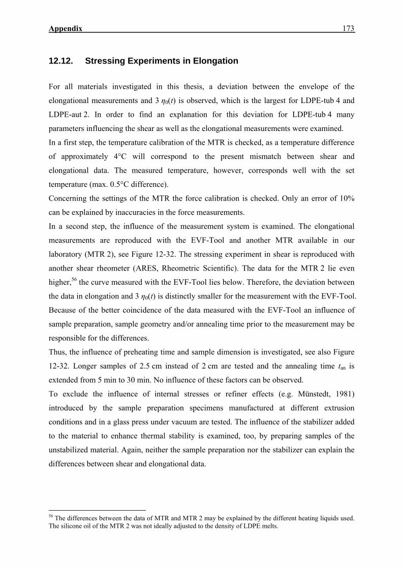
Appendix
173
12.12. Stressing Experiments in Elongation
For all materials investigated in this thesis, a deviation between the envelope of the
elongational measurements and 3 η0(t) is observed, which is the largest for LDPE-tub 4 and
LDPE-aut 2. In order to find an explanation for this deviation for LDPE-tub 4 many
parameters influencing the shear as well as the elongational measurements were examined.
In a first step, the temperature calibration of the MTR is checked, as a temperature difference
of approximately 4°C will correspond to the present mismatch between shear and
elongational data. The measured temperature, however, corresponds well with the set
temperature (max. 0.5°C difference).
Concerning the settings of the MTR the force calibration is checked. Only an error of 10%
can be explained by inaccuracies in the force measurements.
In a second step, the influence of the measurement system is examined. The elongational
measurements are reproduced with the EVF-Tool and another MTR available in our
laboratory (MTR 2), see Figure 12-32. The stressing experiment in shear is reproduced with
another shear rheometer (ARES, Rheometric Scientific). The data for the MTR 2 lie even
higher,56 the curve measured with the EVF-Tool lies below. Therefore, the deviation between
the data in elongation and 3 η0(t) is distinctly smaller for the measurement with the EVF-Tool.
Because of the better coincidence of the data measured with the EVF-Tool an influence of
sample preparation, sample geometry and/or annealing time prior to the measurement may be
responsible for the differences.
Thus, the influence of preheating time and sample dimension is investigated, see also Figure
12-32. Longer samples of 2.5 cm instead of 2 cm are tested and the annealing time tan is
extended from 5 min to 30 min. No influence of these factors can be observed.
To exclude the influence of internal stresses or refiner effects (e.g. Münstedt, 1981)
introduced by the sample preparation specimens manufactured at different extrusion
conditions and in a glass press under vacuum are tested. The influence of the stabilizer added
to the material to enhance thermal stability is examined, too, by preparing samples of the
unstabilized material. Again, neither the sample preparation nor the stabilizer can explain the
differences between shear and elongational data.
56 The differences between the data of MTR and MTR 2 may be explained by the different heating liquids used. The silicone oil of the MTR 2 was not ideally adjusted to the density of LDPE melts.
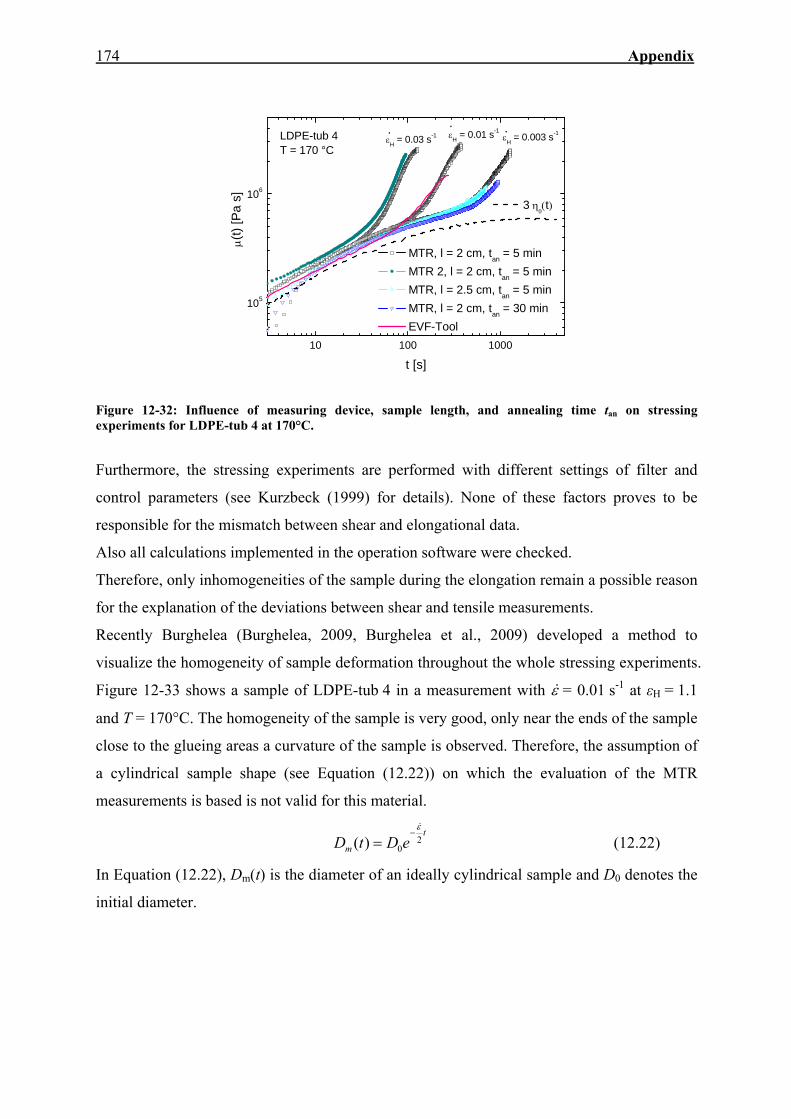
174 Appendix
10 100 1000
105
106
3 η0(t)
MTR, l = 2 cm, tan = 5 min MTR 2, l = 2 cm, tan = 5 min MTR, l = 2.5 cm, tan = 5 min MTR, l = 2 cm, tan = 30 min EVF-Tool
...εH = 0.003 s-1εH = 0.01 s-1
εH = 0.03 s-1
μ(t)
[Pa
s]
t [s]
LDPE-tub 4T = 170 °C
Figure 12-32: Influence of measuring device, sample length, and annealing time tan on stressing experiments for LDPE-tub 4 at 170°C.
Furthermore, the stressing experiments are performed with different settings of filter and
control parameters (see Kurzbeck (1999) for details). None of these factors proves to be
responsible for the mismatch between shear and elongational data.
Also all calculations implemented in the operation software were checked.
Therefore, only inhomogeneities of the sample during the elongation remain a possible reason
for the explanation of the deviations between shear and tensile measurements.
Recently Burghelea (Burghelea, 2009, Burghelea et al., 2009) developed a method to
visualize the homogeneity of sample deformation throughout the whole stressing experiments.
Figure 12-33 shows a sample of LDPE-tub 4 in a measurement with ε& = 0.01 s-1 at εH = 1.1
and T = 170°C. The homogeneity of the sample is very good, only near the ends of the sample
close to the glueing areas a curvature of the sample is observed. Therefore, the assumption of
a cylindrical sample shape (see Equation (12.22)) on which the evaluation of the MTR
measurements is based is not valid for this material.
t
m eDtD 20)(
ε&−
= (12.22)
In Equation (12.22), Dm(t) is the diameter of an ideally cylindrical sample and D0 denotes the
initial diameter.

Appendix
175
Figure 12-33: Homogeneity of LDPE-tub 4 for a measurement with ε& = 0.01 s-1 at εH = 1.1 and T = 170°C (Sample dimensions: l = 2 cm, d = 5 mm).
Based on the curvature of the sample a theory was developed by Burghelea (Burghelea et al.,
2009) to describe the discrepancies between shear and elongational data. The evaluation of
the local diameters along the sample allows the calculation of local stresses. Even small
deviations from the ideal diameter Dm, that are hardly observable by eye, lead to large
changes in the resulting stress. The local stress as a function of experiment time calculated by
the evaluation of the images lies below the integral stress based on an ideally cylindrical
sample. Burghelea finds a very good coincidence between the local stress measurements and
the linear viscoelastic envelope (LVE) from shear data for LDPE-tub 4. Further details
concerning the image analysis and the physical background behind it can be found in
Burghelea (2009), Burghelea et al. (2009), and Burghelea et al. (2009a).
For LDPE-aut 2, which shows the largest deviations between the tensile stressing experiments
and the linear viscoelastic envelope (see Figure 8-1 (b)), stressing experiments with the EVF-
Tool were performed. Figure 12-34 presents transient tensile viscosities measured with the
MTR and the EVF-Tool at different ε& . The accordance of the data measured with the EVF-
Tool and the shear data is very good, whereas for the measurement with the MTR the
deviation between the transient tensile viscosity and the linear viscoelastic envelope is about
60%. This proofs the pronounced effect of an inhomogeneous sample deformation on the
elongational viscosity measured with the MTR.
Three factors are assumed to provide an explanation for the better coincidence of shear data
and elongational data of the EVF-Tool compared to the MTR. One possible reason is the
rectangular sample geometry that might be less sensitive to local thickness fluctuations.
Another reason might be the different way the stress is imposed on the specimen. In the case
of the MTR, one end of the sample is fixed and the other end is pulled up, whereas in the case
of the EVF-Tool the sample is elongated from both ends. As last reason the different sample
lengths used for the determination of the elongational viscosity has to be considered. The
sample volume during the measurement with the MTR is always the same and the length of
the specimen increases exponentially, whereas the sample length during the measurement

176 Appendix
with the EVF-Tool is constant as the two drums of the geometry continuously wind up the
ends of the specimen.
1 10 100 1000
105
106
3 η0(t)
εH = 1 s-1
LDPE-aut 2T = 170 °C
MTR EVF-Tool
μ(t)
[Pa
s]
t [s]
.0.3 s-1
0.1 s-1 0.03 s-1 0.01 s-1
0.005 s-1
0.003 s-1
Figure 12-34: Comparison of transient tensile viscosities μ(t) at different strain rates ε&measured with the MTR and the EVF-tool for LDPE-aut 2.

Appendix
177
12.13. Homogeneity of Deformation in Tensile Creep-Recovery Tests
At the time the creep-recovery experiments were performed, the method of visualizing the
homogeneity of sample deformation throughout the whole experiment had not been installed
yet. Therefore, the deformation of the sample was judged by eye or by taking photographs (of
a rather inferior quality) during the measurement. Additionally the dimensions of the
filaments quenched after the creep-recovery experiments were evaluated. Examples for this
evaluation are presented for measurements on LDPE-tub 4 at 0.5, 5, and 50 kPa in Figure
12-35. Along the length of the sample, the diameter is nearly constant for all measurements
shown. Only at the sample ends close to the plates and near the glueing, however, larger
diameters are observed. The difference between the average diameter and the diameter close
to the plates is the larger the higher the creep stress.
0 2 4 6 8 10 12 14
1.0
1.1
1.2
1.3
d/d m
[-]
l [cm]
0.5 kPa, εH= 1, εr= 0.19 5 kPa, εH= 2.7, εr= 0.90 50 kPa, εH= 3.7, εr= 1.59
LDPE-tub 4T =170°C
Figure 12-35: Sample diameter d as a function of sample length after creep-recovery experiments at a stress of 0.5, 5, and 50 kPa normalized by the average sample diameter dm for LDPE-tub 4.
In Chapter 8.2.2, it is shown that there is a good match of De0 = 1/3 Je
0 despite the deviations
in the relationship μ0 = 3 η0. Since in stressing experiments inhomogeneities in sample
deformation are found to be responsible for the bad correlation between shear and
elongational data the geomotery of the filaments quenched after a creep test, a creep-recovery
test, a stressing experiment, and a stressing experiment with succeeding recovery were
analyzed for LDPE-tub 4. In the creep tests, a stress of 5 kPa was applied. The stressing
experiments were performed with an elongational rate of 0.005 s-1. This rate corresponds to
the average elongational rate during a creep test at 5 kPa. Figure 12-36 gives the results of the

178 Appendix
analysis of geometry of the quenched samples. The homogeneity of the specimen after the
creep test is better than the homogeneity of the specimen after the stressing test. Preliminary
observations of the homogeneity using Burghelea´s technique in a creep test show that the
homogeneity of the sample is much better during the creep measurement than during the
stressing experiment, too (Burghelea, 2009).
The quenched samples after recovery exhibit for both experimental types a comparably good
homogeneity. It seems that the inhomogeneities occurring during the creep and the stressing
test vanish during recovery. As a consequence, the missing inhomogeneities of the retarded
samples may explain the good match of De0 = 1/3 Je
0.
0 5 10 15 20 25 30
0.95
1.00
1.05
1.10
1.15
1.20
1.25
1.30
.
d/d m
[-]
l [cm]
Creep σ = 5 kPa, εH= 2.7 Creep with recovery σ = 5 kPa,
εH= 2.7, εr= 0.90
Stressing ε = 0.005 s-1, εH= 2.7
Stressing with recovery ε = 0.005 s-1, εH= 2.7, εr= 1.02
LDPE-tub 4T =170°C
.
Figure 12-36: Sample diameter d normalized by the average sample diameter dm as a function of sample length after a creep test and a creep-recovery test at a stress of 5 kPa and after a stressing test and a stressing test with succeeding recovery at an elongational rate of 0.005 s-1 for LDPE-tub 4.

Appendix
179
12.14. Abbreviations and Symbols Abbreviations:
aPP atactic PP
DSC differential scanning calorimetry
FT-IR Fourier transformation infrared spectroscopy
HDPE high-density polyethylene
HMS-PP high melt strength polypropylene
iPP isotactic polypropylene
IR infrared
LCB long-chain branched / long-chain branching
LCBrheo long-chain branching determined by rheology
LCBSEC long-chain branching determined by SEC-MALLS
LCB-mLLDPE long-chain branched metallocene linear low-density polyethylene
LCB-PE long-chain branched polyethylene
LCB-PP long-chain branched polypropylene
LDPE low-density polyethylene
LLDPE linear low-density polyethylene
LVE linear viscoelastic envelope
MALLS multi-angle laser light scattering
MFI melt flow index
mHDPE metallocene high-density polyethylene
mLLDPE metallocene linear low-density polyethylene
MMD molar mass distribution
MBR magnetic bearing rheometer
MTR Münstedt tensile rheometer
PE polyethylene
PEEK polyether ether ketone
PET polyethylene terephtalate
PMMA poly(methyl methacrylate)
POM polyoxymethylene
PVC polyvinyl chloride
PP polypropylene
PS polystyrene
RI refractive index
SCB short-chain branching
SEC size exclusion chromatography
sPP syndiotactic polypropylene
TCB 1,2,4-trichlorbenzene
TREF temperature rising elution fractionation
Z/N-LLDPE Ziegler-Natta linear low-density polyethylene
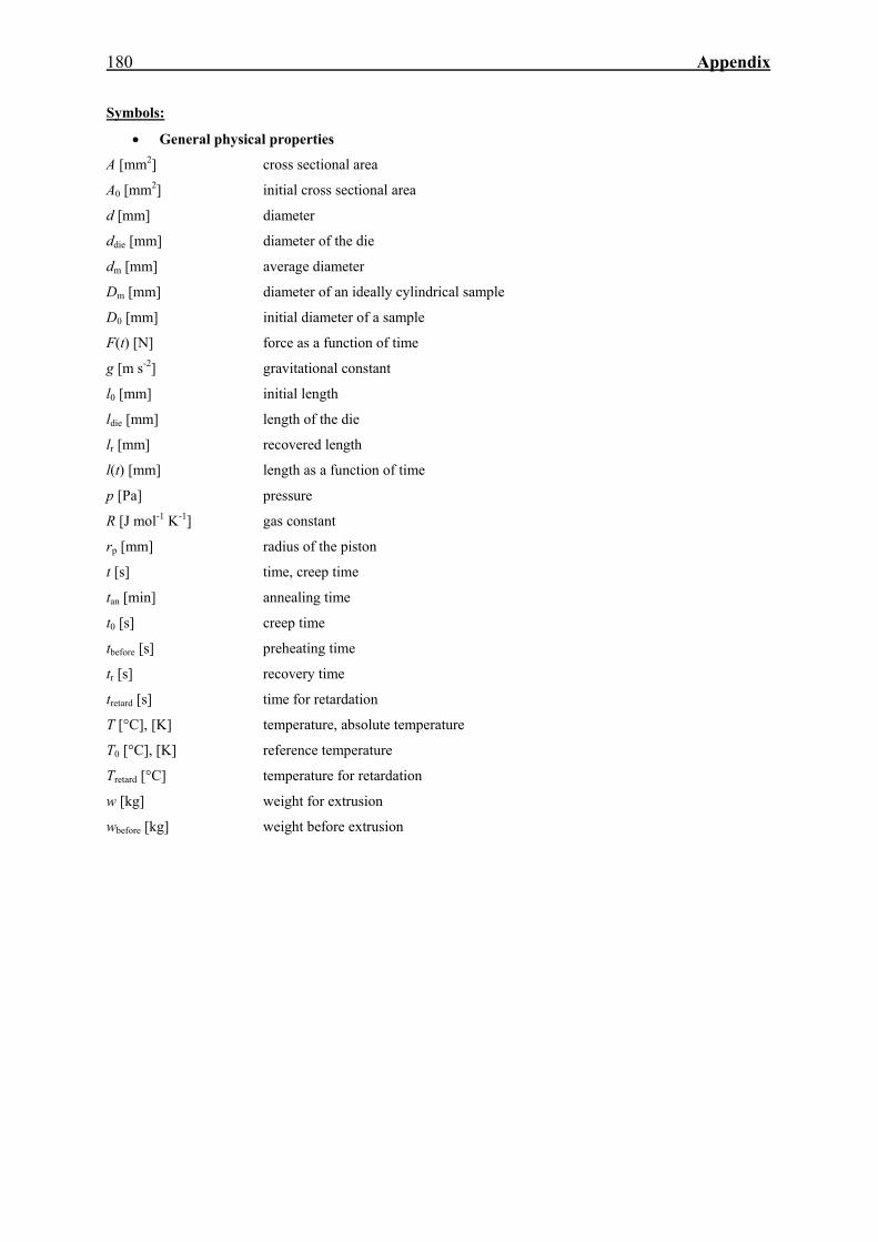
180 Appendix
Symbols:
• General physical properties
A [mm2] cross sectional area
A0 [mm2] initial cross sectional area
d [mm] diameter
ddie [mm] diameter of the die
dm [mm] average diameter
Dm [mm] diameter of an ideally cylindrical sample
D0 [mm] initial diameter of a sample
F(t) [N] force as a function of time
g [m s-2] gravitational constant
l0 [mm] initial length
ldie [mm] length of the die
lr [mm] recovered length
l(t) [mm] length as a function of time
p [Pa] pressure
R [J mol-1 K-1] gas constant
rp [mm] radius of the piston
t [s] time, creep time
tan [min] annealing time
t0 [s] creep time
tbefore [s] preheating time
tr [s] recovery time
tretard [s] time for retardation
T [°C], [K] temperature, absolute temperature
T0 [°C], [K] reference temperature
Tretard [°C] temperature for retardation
w [kg] weight for extrusion
wbefore [kg] weight before extrusion
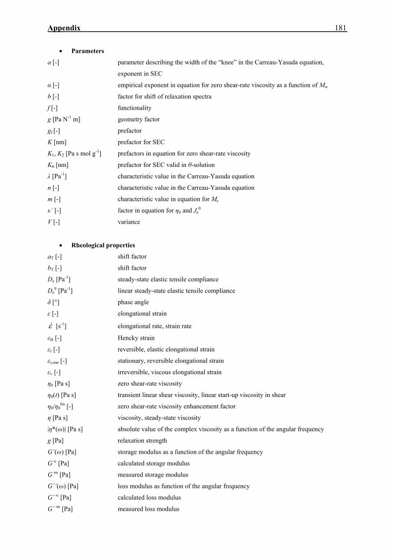
Appendix
181
• Parameters
a [-] parameter describing the width of the “knee” in the Carreau-Yasuda equation,
exponent in SEC
α [-] empirical exponent in equation for zero shear-rate viscosity as a function of Mw
b [-] factor for shift of relaxation spectra
f [-] functionality
g [Pa N-1 m] geometry factor
gf [-] prefactor
K [nm] prefactor for SEC
K1, K2 [Pa s mol g-1] prefactors in equation for zero shear-rate viscosity
Kθ [nm] prefactor for SEC valid in θ-solution
λ [Pa-1] characteristic value in the Carreau-Yasuda equation
n [-] characteristic value in the Carreau-Yasuda equation
m [-] characteristic value in equation for Mc
υ´ [-] factor in equation for η0 and Je0
V [-] variance
• Rheological properties
aT [-] shift factor
bT [-] shift factor
De [Pa-1] steady-state elastic tensile compliance
De0 [Pa-1] linear steady-state elastic tensile compliance
δ [°] phase angle
ε [-] elongational strain
ε& [s-1] elongational rate, strain rate
εH [-] Hencky strain
εr [-] reversible, elastic elongational strain
εr,stat [-] stationary, reversible elongational strain
εv [-] irreversible, viscous elongational strain
η0 [Pa s] zero shear-rate viscosity
η0(t) [Pa s] transient linear shear viscosity, linear start-up viscosity in shear
η0/η0lin [-] zero shear-rate viscosity enhancement factor
η [Pa s] viscosity, steady-state viscosity
|η*(ω)| [Pa s] absolute value of the complex viscosity as a function of the angular frequency
g [Pa] relaxation strength
G´(ω) [Pa] storage modulus as a function of the angular frequency
G´c [Pa] calculated storage modulus
G´m [Pa] measured storage modulus
G´´(ω) [Pa] loss modulus as function of the angular frequency
G´´c [Pa] calculated loss modulus
G´´m [Pa] measured loss modulus

182 Appendix
|G*| [Pa] absolute of the complex modulus
|G*(ω)| [Pa] absolute of the complex modulus as a function of the angular frequency
GN0 [Pa] plateau modulus
G(t) [Pa] linear shear relaxation modulus
G(t,γ) nonlinear shear relaxation modulus
γ& [s-1] shear rate
γ0 [-] maximum deformation, amplitude of deformation
γ [-] shear strain, deformation
γcres [-] additive, residual deformation
γr [-] recoverable deformation
γrmeas [-] experimentally determined deformation
γrtrue [-] unknown (true) recoverable deformation
h(γ) [-] damping function
H(τ) [Pa] relaxation spectrum
J´(ω) [Pa] storage compliance
J´´(ω) [Pa] loss compliance
J0 [Pa-1] instantaneous elastic compliance
Je [Pa-1] steady-state elastic (shear) compliance
Je0 [Pa-1] linear steady-state elastic (shear) compliance
ji [Pa-1] retardation strength
J(t) [Pa-1] creep compliance as a function of creep time
Jr [Pa-1] recoverable compliance
Jr(tr) [Pa-1] recoverable compliance as a function of recovery time
Jrmeas(tr) [Pa-1] measured recoverable compliance as a function of recovery time
Jrtrue(tr) [Pa-1] true recoverable compliance as a function of recovery time
L(τ ) [Pa] retardation spectrum
µ0 [Pa s] linear steady-state tensile viscosity
µs [Pa s] steady-state tensile viscosity
µ(t) [Pa s] transient elongational viscosity
µ0(t) [Pa s] linear transient elongtional viscosity
ω [rad/s], [s-1] angular frequency
ψ(t) [Pa-1] viscoelastic part in the creep experiment
ψ(tr) [Pa-1] viscoelastic part in the recovery experiment
S [-] extrudate swell
S0 [-] equilibrium extrudate swell
σ [Pa] elongational stress
σ(t) [Pa] elongational stress as a function of time
σx [Pa] normal stress in x-direction
σy [Pa] normal stress in y-direction
Tres [nm] residual torque
τ [Pa] shear stress, creep stress
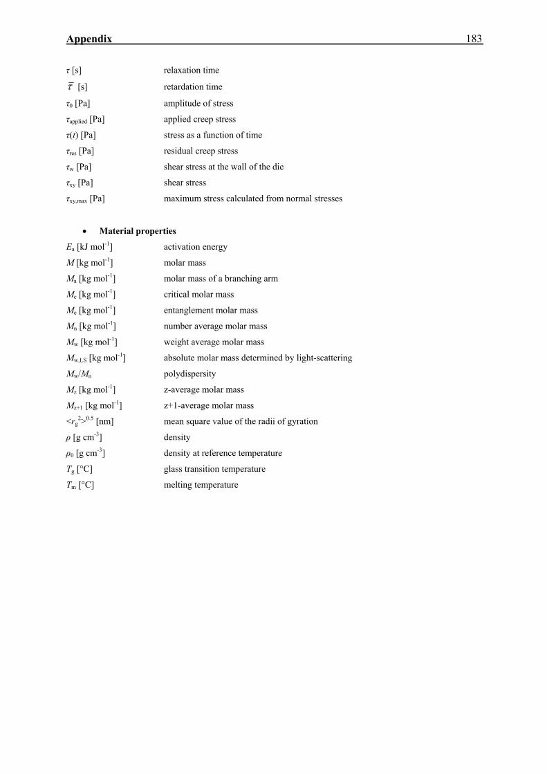
Appendix
183
τ [s] relaxation time
τ [s] retardation time
τ0 [Pa] amplitude of stress
τapplied [Pa] applied creep stress
τ(t) [Pa] stress as a function of time
τres [Pa] residual creep stress
τw [Pa] shear stress at the wall of the die
τxy [Pa] shear stress
τxy,max [Pa] maximum stress calculated from normal stresses
• Material properties
Ea [kJ mol-1] activation energy
M [kg mol-1] molar mass
Ma [kg mol-1] molar mass of a branching arm
Mc [kg mol-1] critical molar mass
Me [kg mol-1] entanglement molar mass
Mn [kg mol-1] number average molar mass
Mw [kg mol-1] weight average molar mass
Mw,LS [kg mol-1] absolute molar mass determined by light-scattering
Mw/Mn polydispersity
Mz [kg mol-1] z-average molar mass
Mz+1 [kg mol-1] z+1-average molar mass
<rg2>0.5 [nm] mean square value of the radii of gyration
ρ [g cm-3] density
ρ0 [g cm-3] density at reference temperature
Tg [°C] glass transition temperature
Tm [°C] melting temperature

184 References
13. References Agarwal P. K., Plazek D. J. (1977) Shear creep recovery behaviour of IUPAC low-density polyethylenes. Journal of Applied Polymer Science 21 (12): 3251-3260 Agarwal P. K. (1979) A relationship between steady state shear compliance and molecular weight distribution. Macromolecules 12 (2): 342-344 Archer L. A. (1999) Separability criteria for entangled polymer liquids. Journal of Rheology 43 (6): 1555-1571 Auhl D., Stange J., Münstedt H., Krause B., Voigt D., Lederer A., Lappan U., Lunkwitz K. (2004) Long-chain branched polypropylenes by electron beam irradiation and their rheological properties. Macromolecules 37 (14): 9465-9472 Auhl D. W. (2006) Molekulare Struktur und rheologische Eigenschaften strahlenmodifizierter Polypropylene. Ph.D.-Thesis, Friedrich-Alexander-Universität Erlangen-Nürnberg Auhl D., Ramirez J., Likhtman A. E., Chambon P., Fernyhough C. (2008) Linear and non-linear shear flow behavior of monodisperse polyisoprene melts with a large range of molecular weights. Journal of Rheology 52 (3): 801-835 Ball R. C., McLeish T. C. B. (1989) Dynamic dilution and the viscosity of star-polymer melts. Macromolecules 22 (4): 1911-1913 Baumgärtel M., Winter H. H. (1989) Determination of discrete relaxation and retardation time spectra from dynamic mechanical data. Rheologica Acta 28 (6): 511-519
Bin Wadud S. E., Baird D. G. (2000) Shear and extensional rheology of sparsely branched metallocene-catalyzed polyethylenes. Journal of Rheology 44 (5): 1151-1167 Bird B., Armstrong R. C., Hassager O.: Dynamics of polymeric liquids, Volume 1: Fluid mechanics. John Wiley & Sons, New York, 1987 Burghelea T. (2009) Personal communication Burghelea T., Stary Z., Münstedt H. (2009) Local versus integral measurements of the extensional viscosity of polymer melts. Journal of Rheology, accepted Burghelea T., Stary Z., Münstedt H. (2009a) The viscosity overshoot during the uniaxial extension of a low density polyethylene. Journal of Rheology, submitted
Carella J. M., Graessley W. W., Fetters L. J. (1984) Effects of chain microstructure on the viscoelastic properties of linear polymer melts: polybutadienes and hydrogenated polybutadienes. Macromolecules 17 (12): 2775-2786 Carreau P. (1968) Rheological equations from molecular network theories. Ph.D.-Thesis, University of Wisconsin, Madison Chou, P. C., Pagano N. J.: Elasticity – Tensor, Dyadic, and Engineering approaches. Dover Publications Inc., New York, 1992 Cogswell F. (1975) Polymer melt rheology during elongational flow. Applied Polymer Symposium 27: 1-18 Costeux S., Wood-Adams P. M., Beigzadeh D. (2002) Molecular structure of metallocene-catalyzed polyethylene: Rheologically relevant representation of branching architecture in single catalyst and blended systems. Macromolecules 35 (7): 2514-2528 Dealy J. M., Larson R. G.: Structure and rheology of molten polymers. Carl Hanser Verlag, München, 2006

References
185
Den Doelder J. (2006) Viscosity and compliance from molar mass distribution using double reptation models. Rheologica Acta 46 (2): 195-210 Derfuß B. (2003) Rheologische Untersuchungen an langkettenverzweigten Polypropylenen. Diploma-Thesis, Friedrich-Alexander-Universität Erlangen-Nürnberg Doi M., Edwards S. F.: The theory of polymer dynamics. Clarendon Press, Oxford, 1986 Domininghaus H., Elsner P., Eyerer P., Hirth T.: Kunststoffe – Eigenschaften und Anwendungen, 7. Auflage. Springer Verlag, Berlin-Heidelberg, 2008 Eckstein A., Friedrich C., Lobbrecht A., Spitz R. (1997) Comparison of the viscoelastic properties of syndio- and isotactic polypropylenes. Acta Polymerica 48 (1-2): 41-46 Eckstein A., Suhm J., Friedrich C., Maier R.-D., Sassmannshausen J., Bochmann M., Mülhaupt R. (1998) Determination of plateau moduli and entanglement molecular weights of isotactic, syndiotactic, and atactic polypropylenes synthesized with metallocene catalysts. Macromolecules 31 (4): 1335-1340 Ferry J. D. (1950) Mechanical properties of substances of high molecular weight. VI. Dispersion in concentrated polymer solutions and its dependence on temperature and concentration. Journal of American Chemical Society 72 (8): 3746-3752 Ferry J. D.: Viscoelastic properties of polymers, 3rd edn. Wiley and Sons, New York, 1980 Fetters L. J., Kiss A. D., Pearson D. S., Quack G. F., Vitus F. J. (1993) Rheological behavior of star-shaped polymers. Macromolecules 26 (4): 647-654 Fetters L. J., Lohse D. J., Graessley W. W. (1999) Chain dimensions and entanglement spacings in dense macromolecular systems. Journal of Polymer Science: Part B, Polymer Physics 37 (10): 1023-1033 Fleissner, von M. (1973) Die Schwellrate von Polyäthylenschmelzen in Relation zu molekularen Parametern. Die Angewandte Makromolekulare Chemie 33 (1): 75-87 Fuchs K., Friedrich C., Weese J. (1996) Viscoelastic properties of narrow-distribution poly(methylmethacrylates). Macromolecules 29 (18): 5893-5901 Fujiyama J., Awaya H. (1972) Relationship in polypropylene melt between its linear viscoelasticity and its steady capillary flow properties. Journal of Applied Polymer Science 16 (2): 275-299 Fujiyama M., Inata H. (2002) Rheological properties of metallocene isotactic polypropylenes. Journal of Applied Polymer Science 84 (12): 2157-2170 Fujiyama M., Kitajima Y., Inata H. (2002) Rheological properties of polypropylenes with different molecular weight distribution characteristics. Journal of Applied Polymer Science 84 (12): 2128-2141 Frater D. J., Mays J. W., Jackson C. (1997) Synthesis and dilute solution properties of divinylbenzene-linked polystyrene stars with mixed arms lengths: Evidence for coupled stars. Journal of Polymer Science: Part B, Polymer Physics 35 (1): 141-151 Gabriel C., Kaschta J. (1998) Comparison of different shear rheometers with regard to creep and creep recovery measurements. Rheologica Acta 37 (4): 358–364 Gabriel C., Kaschta J., Münstedt H. (1998) Influence of molecular structure on rheological properties of polyethylenes I. Creep recovery measurements in shear. Rheologica Acta 37 (1): 7-20 Gabriel C., Münstedt H. (1999) Creep recovery behavior of metallocene linear low-density polyethylenes. Rheologica Acta 38 (5): 393-403 Gabriel C. (2001) Einfluss der molekularen Struktur auf das viskoelastische Verhalten von Polyethylenschmelzen. Ph.D.-Thesis, Friedrich-Alexander-Universität Erlangen-Nürnberg
186 References
Gabriel C., Münstedt H. (2002) Influence of long-chain branches in polyethylenes on linear viscoelastic flow properties in shear. Rheologica Acta 41 (3): 232-244 Gabriel C., Kokko E., Löfgren B., Seppälä J., Münstedt H. (2002) Analytical and rheological characterization of long-chain branched metallocene-catalyzed ethylene homopolymers. Polymer 43 (24): 6383-6390 Gabriel C., Münstedt H. (2003) Strain hardening of various polyolefins in uniaxial elongational flow. Journal of Rheology 47 (3): 619-630 Gahleitner M. (2001) Melt rheology of polyolefins. Progress in Polymer Science 26 (6): 895-944 Goyal S. K., Bohnet N., Aubee N. (1995) LLDPE/LDPE Blends: Effect of composition on the rheological and physical properties. Proceedings of 53rd Antec Conference: 3221-3227 Graessley W.W.: The entanglement concept in polymer rheology. Springer Verlag, Berlin-Heidelberg, 1974 Graessley W. W., Roovers J. (1979) Melt rheology of four-arm and six-arm star polystyrenes. Macromolecules 12 (5): 959–965 Graessley W. W., Edwards S. F. (1981) Entanglement interactions in polymers and the chain contour concentration. Polymer 22 (10): 1329-1334 Graessley W. W., Struglinski M. J. (1986) Effects of polydispersity on the linear viscoelastic properties of entangled polymers. 2. Comparison of viscosity and recoverable compliance with tube model predictions. Macromolecules 19 (6): 1754-1760 Gramespacher H., Meissner J. (1997) Melt elongation and recovery of polymer blends, morphology, and influence of interfacial tension. Journal of Rheology 41 (1): 27-44 Groto J. T., Graessley W. W. (1984) Model hydrocarbon polymers: Rheological properties of linear polyisoprenes and hydrogenated polyisoprenes. Macromolecules 17 (12): 2767-2775 Gubler M. G., Kovacs A. J. (1959) La structure du polyéthylène consideré comme un mélange de n-paraffines. Journal of Polymer Science 34 (127): 551-568 Hepperle J. (2002) Einfluss der molekularen Struktur auf rheologische Eigenschaften von Polystyrol- und Polycarbonatschmelzen. Ph.D.-Thesis, Friedrich-Alexander-Universität Erlangen-Nürnberg Hepperle J., Münstedt H. (2006) Rheological properties of branched polystyrenes: nonlinear shear and extensional behavior. Rheologica Acta 45 (5): 717-727 Hingmann R., Marczinke B. (1994) Shear and elongational flow properties of polypropylene melts. Journal of Rheology 38 (3): 573-587 Hughes R. H. (1969) The determination of the isotacticity of polypropylene in the 90-100% range by infrared spectroscopy. Journal of Applied Polymer Science 13 (3): 417-425 Ishizuka O., Koyama K. (1980) Elongational viscosity at a constant elongational strain rate of polypropylene melt. Polymer 21 (2): 164-170 Janzen J., Colby R. H. (1999) Diagnosing long-chain branching in polymers. Journal of Molecular Structure 485-486: 569-584 Jordens K., Wilkes G. L., Janzen J., Rohlfing D. C., Welch M. B. (2000) The influence of molecular weight and thermal history on the thermal, rheological, and mechanical properties of metallocene-catalyzed linear polyethylenes. Polymer 41 (19): 7175-7192 Kar K. K., Otaigbe J. U. (2001) Numerical analysis and experimental studies on the role of rheological properties in effecting die swell of low density polyethylene, polypropylene and polystyrene: A predictive model based on Newtonian fluid. Journal of Elastomers and Plastics 33 (4): 297-336
References
187
Kaschta J., Schwarzl F. R. (1994) Calculation of discrete retardation spectra from creep data – I. Method. Rheologica Acta 33 (6): 517-529 Kaschta J., Schwarzl F. R. (1994a) Calculation of discrete retardation spectra from creep data – II. Analysis of measured creep curves. Rheologica Acta 33 (6): 530-541 Kaschta J., Stadler F. J. (2009) Avoiding waviness of relaxation spectra. Rheologicy Acta 48 (6): 709-713 Kasehagen L. J., Macosko C. W. (1998) Nonlinear shear and extensional rheology of long-chain randomly branched polybutadiene. Journal of Rheology 42 (6): 1303-1327
Kazatchkov I. B., Bohnet H., Goyal S. K., Hatzikiriakos S. G. (1999) Influence of molecular structure on the rheological and processing behaviour of polyethylene resins. Polymer Engineering and Science 39 (4): 804-815 Keim W.: Kunststoffe, Synthese, Herstellungsverfahren, Apparaturen. Wiley-VCH, Berlin-Heidelberg, 2006 Keßner U., Kaschta J., Münstedt H. (2009) Determination of method-invariant activation energies of long-chain branched low density polyethylene. Journal of Rheology 53 (4): 1001-1016 Koopmans R. J. (1992) Extrudate swell of high density polyethylene. Part 1: Aspects of molecular structure and rheological characterization methods. Polymer Engineering and Science 32 (23): 1741-1749 Koyama K., Ishizuka O. (1981) The influence of molecular weight distribution on elongational flow of polyethylene. Sen´I Gakkaishi 37 (6): 258-261 Kurata M., Osaki K., Einaga Y., Sugie T. (1974) Effect of molecular weight distribution on viscoelastic properties of polymers. Journal of Polymer Science: Part B, Polymer Physics 12 (5): 849-869 Kurata M. (1984) Effect of molecular weight distribution on viscoelastic properties of polymers. 2. Terminal relaxation time and steady-state compliance. Macromolecules 17 (4): 895–898 Kurzbeck S. (1999) Dehnrheologische Eigenschaften von Polyolefinschmelzen und Korrelation mit ihrem Verarbeitungsverhalten beim Folienblasen und Thermoformen. Ph.D.-Thesis, Friedrich-Alexander-Universität Erlangen-Nürnberg Kurzbeck S., Oster F., Münstedt H., Nguyen T. Q., Gensler R. (1999) Rheological properties of two polypropylenes with different molecular structure. Journal of Rheology 43 (2): 359-374 Krause B., Voigt D., Häußler L., Auhl D., Münstedt H. (2006) Characterisation of electron beam irradiated polypropylene: Influence of irradiation temperature on molecular and rheological properties. Journal of Applied Polymer Science 100 (4): 2770-2780 Lagendijk R. P., Hogt A. H., Buijtenhuijs A., Gotsis A. D. (2001) Peroxydicarbonate modification of polypropylene and extensional flow properties. Polymer 42 (25): 10035-10043 Laun H. M., Münstedt H. (1978) Elongational behaviour of a low density polyethylene melt. I. Strain rate dependence of viscosity and recoverable strain in the steady state. Comparison with shear data. Influence of interfacial tension. Rheologica Acta 17 (4): 415-425 Laun H. M. (1987) Orientation of macromolecules and elastic deformations in polymer melts. Influence of molecular structure on the reptation of molecules. Progress in Colloid & Polymer Science 75 (1): 111-136 Le Guillou J. C., Zinn-Justin J. (1977) Critical exponents for the n-vector model in three dimensions from field theory. Physical Review Letters 39 (2): 95-98 Liang J. Z., Ness J. N. (1998) The melt die-swell behaviour during capillary extrusion of LDPE/PP blends. Polymer Testing 17 (3): 179-189 Liang J. Z. (2002) The elastic behaviour during capillary extrusion of LDPE/LLDPE blend melts. Polymer Testing 21 (1): 69-74
188 References
Lieberman R. B., LeNoir R. T: Manufacturing. In: Moore, Jr. E. P.: Polypropylene Handbook. Carl Hanser Verlag, München, 287-303, 1996 Link G., Schwarzl F. R. (1985) Measuring device for precise evaluation of torsional creep and recovery data. Rheologica Acta 24 (3): 211-219 Lohse D. J., Milner S. T., Fetters L. J., Xenidou M., Hadjichristidis N., Roovers J., Mendelson R. A., Garcia-Franco C. A., Lyon M. K. (2002) Well-defined, model long chain branched polyethylene. 2. Melt rheological behavior. Macromolecules 35 (8): 3066-3075 Machui F. (2009) Morphologieentwicklung in Schmelzen aus Polystyrol / Polyethylen Blends unter Dehnbeanspruchung. Diploma-Thesis, Friedrich-Alexander-Universität Erlangen-Nürnberg Malmberg A., Liimaatta J., Lehtinen A., Löfgren B. (1999) Characteristics of long chain branching in ethene polymerization with single site catalysts. Macromolecules 32 (20): 6687-6696 Malmberg A., Gabriel C., Steffl T., Münstedt H., Löfgren B. (2002) Long-chain branching in metallocene-catalyzed polyethylenes investigated by low oscillatory shear and uniaxial extensional rheometery. Macromolecules 35 (3): 1038-1048 Masuda T., Kitagawa K., Inoue T., Onogi S. (1970) Rheological properties of anionic polystyrenes. II. Dynamic viscoelasticity of blends of narrow-distribution polystyrenes. Macromolecules 3 (2): 116-125 Mavridis H., Shroff R. N. (1992) Temperature dependence of polyolefin melt rheology. Polymer Engineering and Science 32 (23): 1778-1792 McLeish T. C. B., Milner S. T. (1999) Entangled dynamics and melt flow of branched polymers. Advances in Polymer Science 143: 195-256 Meissner J. (1972) Development of a universal extensional rheometer for the uniaxial extension of polymer melts. Transactions of the Society of Rheology 16 (3): 405-420 Meissner J. (1975) Zur Temperaturunabhängigkeit elastischer Erscheinungen bei der Scherung von Kunststoff-Schmelzen im nicht-linearen Deformationsbereich. Rheologica Acta 14 (5): 471-473 Meissner J. (1984) Polymer melt rheology – a challenge for the polymer scientist and engineer. Pure and Applied Chemistry 56 (3): 369-384 Mills N. J. (1969) The rheological properties and molecular weight distribution of polydimethylsiloxane. European Polymer Journal 5 (5): 675-695 Minegishi A., Nishioka A., Takahashi T., Masubuchi Y., Takimoto J., Koyama K. (2001) Uniaxial elongational viscosity of PS / a small amount of UHMW-PS blends. Rheologica Acta 40 (4): 329-338 Minoshima W., White J. L., Spruiell J. E. (1980) Experimental investigations of the influence of molecular weight distribution on the rheological properties of polypropylene melts. Polymer Science and Engineering 20 (17): 1166-1176 Minoshima W., White J. L., Spruiell J. E. (1980a) Experimental investigations of the influence of molecular weight distribution on melt spinning and extrudate swell characteristics of polypropylene. Journal of Applied Polymer Science 25 (2): 287-306 Mori S., Barth H. G.: Size exclusion chromatography. Springer Verlag, Berlin-Heidelberg-New York, 1999 Münstedt H. (1975) Viscoelasticity of polystyrene melts in tensile creep experiments. Rheologica Acta 14 (12): 1077-1088 Münstedt H., Laun H. M. (1979) Elongational behaviour of a low density polyethylene melt. II. Transient behaviour in constant stretching rate and tensile creep experiments. Comparison with shear data. Temperature dependence of the elongational properties. Rheologica Acta 18 (4): 492-504

References
189
Münstedt H. (1980) Dependence of the elongational behavior of polystyrene melts on molecular weight and molecular weight distribution. Journal of Rheology 24 (6): 847-867 Münstedt H., Laun H. M. (1981) Elongational properties and molecular structure of polyethylene melts. Rheologica Acta 20 (3): 211-221 Münstedt H. (1981) The influence of various deformation histories on elongational properties of low density polyethylene. Colloid and Polymer Science 259 (10): 966-972 Münstedt H.: Polymerschmelzen. In: W.-M. Kulicke: Fließverhalten von Stoffen und Stoffgemischen. Hüthig und Wepf, Basel, 238-279, 1986 Münstedt H., Kurzbeck S., Egersdörfer L. (1998) Influence of molecular structure on rheological properties of polyethylenes. Part II. Elongational behavior. Rheologica Acta 37 (1): 21-29 Münstedt H., Auhl D. W. (2005) Rheological measuring techniques and their relevance for the molecular characterization of polymers. Journal of Non-Newtonian Fluid Mechanics 128 (1): 62-69 Münstedt H., Katsikis N., Kaschta J. (2008) Rheological properties of poly(methyl methacrylate)/nanoclay composites as investigated by creep recovery in shear. Macromolecules 41 (24): 9777-9783 Nam G. J., Yoo J. H., Lee J. W. (2005) Effect of long-chain branches of polypropylene on rheological properties and foam-extrusion performances. Journal of Applied Polymer Science 96 (5): 1793-1800 Nemoto N. (1970) Viscoelastic properties of narrow-distribution polymers. II. Tensile creep studies of polystyrene. Polymer Journal 1 (4): 485-492 Onogi S., Masuda T., Kitagawa K. (1970) Rheological properties of anionic polystyrenes. I. Dynamic viscoelasticity of narrow-distribution polystyrenes. Macromolecules 3 (2): 109-116 Orbon S. J., Plazek D. J. (1979) Recoverable compliance of a series of bimodal molecular weight blends of polystyrene. Journal of Polymer Science: Polymer Physics Edition 17 (11): 1871-1890 Patham B., Jayaraman K. (2005) Creep recovery of random ethylene-octene copolymer melts with varying comonomer content. Journal of Rheology 49 (5): 989-999 Pearson D. S., Helfand E. (1984) Viscoelastic properties of star-shaped polymers. Macromolecules 17 (4): 888-895 Pechhold W., v. Soden W., Stoll B. (1981) Shear compliance of polymer melts and its dependence on molecular weight. Die Makromolekulare Chemie 182 (2): 573-581 Phillips R. A., Wolkowicz M. D.: Structure and Morphology. In: Moore, Jr. E. P.: Polypropylene Handbook. Carl Hanser Verlag, München, 287-303, 1996 Piel C., Stadler F. J., Kaschta J., Rulhoff S., Münstedt H., Kaminsky W. (2006) Structure-property relationships of linear and long-chain branched metallocene high-density polyethylenes characterized by shear rheology and SEC-MALLS. Macromolecular Chemistry and Physics 207 (1): 26-38 Plazek D. J. (1968) Magnetic-bearing torsional creep apparatus. Journal of Polymer Science: Part A-2, Polymer Physics 6 (3): 621-638 Plazek D. J., O´Rourke V. M. (1971) Viscoelastic behavior of low molecular weight polystyrene. Journal of Polymer Science: Part A-2, Polymer Physics 9 (2): 209-243 Plazek D. J., Raghupathi N., Kratz R. F., Miller W. R. (1979) Recoverable compliance behavior of high-density polyethylenes. Journal of Applied Polymer Sciene 24 (5): 1305-1320 Plazek D. J.: The creep behaviour of amorphous polymers. In: Ngai K. L., Wright G. B.: Relaxation in complex systems. Naval Research Laboratory Washington, 83-109, 1984
190 References
Podzimek S., Vlcek T., Johann C. (2001) Characterization of branched polymers by size exclusion chromatography coupled with multiangle light scattering detector. I. Size exclusion chromatography elution behavior of branched polymers. Journal of Applied Polymer Science 81 (7): 1588-1594 Raju V. R., Smith G. G., Marin G., Know J. R., Graessley W. W. (1979) Properties of amorphous and crystallizable hydrocarbon polymers. I. Melt rheology of fractions of linear Polyethylene. Journal of Polymer Science: Part B, Polymer Physics 17 (7): 1183-1195 Resch J. A., Stadler F. J., Kaschta J., Münstedt H. (2009) Temperature dependence of the linear steady-state shear compliance of linear and long-chain branched polyethylenes. Macromolecules 42 (15): 5676-5683 Rochefort W. E., Smith G. G., Rachapudy H., Raju V. R., Graessley W. W. (1979) Properties of amorphous and crystallisable hydrocarbon polymers. II. Rheology of linear and star-branched polybutadiene. Journal of Polymer Science: Part B, Polymer Physics 17 (7): 1197-1210 Rogers M. G. (1970) Some studies on the swelling behaviour of polyethylene. Journal of Applied Polymer Science 14 (7): 1679-1689 Rojo E., Muñoz M. E., Santamaria A., Peña B. (2004) Correlation between conformational parameters and rheological properties of molten syndiotactic polypropylenes. Macromolecular Rapid Communications 25 (14): 1314-1318 Romanini D., Savadori A., Gianotti G. (1980) Long chain branching in low density polyethylene: 2. Rheological behaviour of polymers. Polymer 21 (9): 1092-1101 Romanini D., Pezzin G. (1982) Relation between extrudate swelling of polypropylene and molecular weight. Rheologica Acta 21 (6): 699-704 Roovers J., Graessley W. W. (1981) Melt rheology of some model comb polystyrenes. Macromolecules 14 (3): 766–773 Roovers J. (1984) Melt rheology of H-shaped polystyrenes. Macromolecules 17 (6): 1196-1200 Roovers J., Toporowski P. M. (1987) Relaxation by constraint release in combs and star-combs. Macromolecules 20 (9): 2300-2306 Scheve B., Mayfield J. W., DeNicola A. J. (1986) Polypropylene mit freier Langkettenverzweigung, Verfahren zur Herstellung und Verwendung davon. EP0190889 Schwarzl F. R. (1970) On the interconversion between viscoelastic material functions. Pure and Applied Chemistry 23 (2-3): 219-234 Schwarzl F. R.: Polymermechanik – Struktur und mechanisches Verhalten von Polymeren. Springer Verlag, Berlin-Heidelberg, 1990 Schwarzl F. R. (2008) Personal communication Sinn H., Kaminsky W. (1980) Ziegler-Natta-Catalysis. Advances in Organometallic Chemistry 18: 99-149 Simak P. (1988) Spektroskopische Bestimmung von Ethylen in Ethylen-Propylen-Copolymeren. Kunststoffe 78 (3): 234-236 Stange J. (2006) Einfluss rheologischer Eigenschaften auf das Schäumverhalten von Polypropylenen unterschiedlicher molekularer Struktur. Ph.D.-Thesis, Friedrich-Alexander-Universität Erlangen-Nürnberg Stadler F. J., Kaschta J., Münstedt H. (2005) Dynamic-mechanical behavior of polyethylenes and ethene-/α-olefin-copolymers: Part I: α’-relaxation. Polymer 46 (23): 10311-10320 Stadler F. J., Piel C., Kaschta J., Rulhoff S., Kaminsky W., Münstedt H. (2006) Dependence of the zero shear-rate viscosity and the viscosity function of linear high density polyethylenes on the mass-average molar mass and polydispersity. Rheologica Acta 45 (5): 755-764

References
191
Stadler F. J., Piel C., Klimke K., Kaschta J., Parkinson M., Wilhelm M., Kaminsky W., Münstedt H. (2006a) Influence of type and content of various comonomers on long-chain branching of ethene/α-olefin copolymers. Macromolecules 39 (4): 1474-1482 Stadler F. J. (2007) Molecular structure and rheological properties of linear and long-chain branched ethene-/α-olefin copolymers. Ph.D.-Thesis, Friedrich-Alexander-Universität Erlangen-Nürnberg Stadler F. J., Gabriel C., Münstedt H. (2007) Influence of short-chain branching of polyethylenes on the temperature dependence of rheological properties in shear. Macromolecular Chemistry and Physics 208 (22): 2449-4454 Stadler F. J., Kaschta J., Münstedt H. (2008) Thermorheological behavior of various long-chain branched polyethylenes. Macromolecules 41 (4): 1328-1333 Stadler F. J., Münstedt H. (2008) Terminal viscous and elastic properties of linear ethene-/α-olefin copolymers. Journal of Rheology 52 (3): 697-712 Stadler F. J., Bailly C. (2009) A new method for the calculation of continuous relaxation spectra from dynamic-mechanical data. Rheologica Acta 48 (1): 33-49 Stadler F. J. (2009) Personal communication
Struglinski M. J., Graessley W. W., Fetters L. J. (1988) Effects of polydispersity on the linear viscoelastic properties of entangled polymers. 3. Experimental observations on binary mixtures of linear and star polybutadienes. Macromolecules 21 (3): 783-789 Sun T., Brant P., Chance R. R., Graessley W. W. (2001) Effect of short chain branching on the coil dimensions of polyolefins in dilute solution. Macromolecules 34 (19): 6812-6820 Takahashi M., Isaki T., Takigawa T., Masuda T. (1993) Measurement of biaxial and uniaxial extensional flow behavior of polymer melts at constant strain rates. Journal of Rheology 37 (5): 827-846 Tackx P., Tacx J. C. J. F. (1998) Chain architecture of LDPE as a function of molar masss using size exclusion chromatography and multi-angle laser light scattering (SEC-MALLS). Polymer 39 (14): 3109-3113
Trinkle S., Friedrich C. (2001) Van Gurp-Palmen-plot: a way to characterize polydispersity of linear polymers. Rheologica Acta 40 (4): 322-328 Trinkle S., Walter P., Friedrich C. (2002) Van Gurp-Palmen-Plot II – classification of long chain branched polymers by their topology. Rheologica Acta 41 (1-2): 103-113 Trzebiatowski T., Wilski H. (1985) Die Dehnviskosität des Polypropylens. Rheologica Acta 24 (6): 582-587 Tsenoglou C. J., Gotsis A. D. (2001) Rheological characterization of long chain branching in a melt of evolving molecular architecture. Macromolecules 34 (14): 4685-4687 Utracki L. A., Schlund B. (1987) Linear low density polyethylenes and their blends: Part 1. Molecular characterization. Polymer Engineering and Science 27 (5): 359-366 Utracki L. A., Schlund B. (1987a) Linear low density polyethylenes and their blends: Part 2. Shear flow of LLDPE's. Polymer Engineering and Science 27 (5): 367-379 Van Gurp M., Palmen J. (1998) Time-temperature superposition for polymeric blends. Rheology Bulletin 67 (1): 5-8 Vega J. F., Santamaría A., Muñoz-Escalona A., Lafuente P. (1998) Small-amplitude oscillatory shear flow measurements as a tool to detect very low amounts of long chain branching in polyethylenes. Macromolecules 31 (11): 3639-3647 Vega J. F., Fernández M., Santamaría A., Muñoz-Escalona A., Lafuente P. (1999) Rheological criteria to characterize metallocene catalyzed polyethylenes. Macromolecular Chemistry and Physics 200 (10): 2257-2268

192 References
Wagner M. H. (1976) Analysis of time-dependent non-linear stress-growth data for shear and elongational flow of a low-density branched polyethylene melt. Rheologica Acta 15 (2): 136-142 Wagner M. H., Laun H. M. (1978) Nonlinear shear creep and constrained elastic recovery of a LDPE melt. Rheologica Acta 17 (2): 138-148 Wagner M. H., Ehrecke P., Hachmann P., Meissner J. (1998) A constitutive analysis of unixial, equibiaxial and planar extension of a commercial linear high-density polyethylene melt. Journal of Rheology 42 (3): 621-638 Wagner M. H., Bastian H., Hachmann P., Meissner J., Kurzbeck S., Münstedt H., Langouche F. (2000) The strain-hardening behaviour of linear and long-chain branched polyolefin melts in extensional flows. Rheologica Acta 39 (2): 97-109 Wagner M. H., Rubio P., Bastian H. (2001) The molecular stress function model for polydisperse polymer melts with dissipative convective constraint release. Journal of Rheology 45 (6): 1387-1412 Wagner M. H., Yamaguchi M., Takahashi M. (2003) Quantitative assessment of strain hardening of low-density polyethylene melts by the molecular stress function model. Journal of Rheology 74 (3): 779-793
Walter P., Trinkle S., Lilge D., Friedrich C., Mülhaupt R. (2001) Long chain branched polypropylene prepared by means of propene copolymerization with 1,7-octadiene using MAO-activated rac-Me2Si(2-Me-Phenyl-Ind)2ZrCl2. Macromolecular Material Engineering 286 (5): 309-315 Wasserman S. H., Graessley W. W. (1996) Prediction of linear viscoelastic response for entangled polyolefin melts from molecular weight distribution. Polymer Engineering and Science 36 (6): 852-861 Weng W., Hu W., Dekmezian A. H., Ruff C. J. (2002) Long chain branched isotactic polypropylene. Macromolecules 35 (10): 3838–3843 Wolf B., Kenig S., Klopstock J., Miltz J. (1996) Thermal fractionation and identification of low-density polyethylenes. Journal of Applied Polymer Science 62 (9): 1339-1345 Wolff F. (2008) Einfluss molekularer Parameter auf elastische Eigenschaften von Polypropylenen in Scherung und Dehnung. Diploma-Thesis, Friedrich-Alexander-Universität Erlangen-Nürnberg Wolff F., Resch J. A., Kaschta J., Münstedt H. (2010) Comparison of viscous and elastic properties of polyolefin melts in shear and elongation. Rheologica Acta 49 (1): 95-103 Wood-Adams P. M., Dealy J. M. (2000) Using rheological data to determine the branching level in metallocene polyethylenes. Macromolecules 33 (20): 7481-7488 Wood-Adams P., Dealy J. M., deGroot A. W., Redwine O. D. (2000) Effect of molecular structure on the linear viscoelastic behavior of polyethylene. Macromolecules 33 (20): 7489-7499 Wood-Adams P. M. (2001) The effect of long chain branches on the shear flow behavior of polyethylene. Journal of Rheology 45 (1): 203-210 Wood-Adams P. M., Costeux S. (2001) Thermorheological behavior of polyethylene: Effects of microstructure and long chain branching. Macromolecules 34 (18): 6281-6290 Yamaguchi M., Takahashi M. (2001) Rheological properties of low-density polyethylenes produced by tubular and vessel processes. Polymer 42 (21): 8663-8670
Yan D., Wang W.-J., Zhu S. (1999) Effect of long chain branching on rheological properties of metallocene polyethylene. Polymer 40 (7): 1737-1744 Yasuda K. (1979) Investigation of the analogies between viscometric and linear viscoelastic properties of polystyrene. Ph.D.-Thesis, MIT, Cambridge Yoshii F., Makuuchi K., Kikukawa S., Tanaka T., Saitoh J., Koyama K. (1996) High-melt-strength polypropylene with electron beam irradiation in the presence of polyfunctional monomers. Journal of Applied Polymer Science 60 (4): 617-623

References
193
Zimm B. H. (1948) Apparatus and methods for measurement and interpretation of the angular variation of light scattering; preliminary results on polystyrene solutions. Journal of Chemical Physics 16 (12): 1099-1116 Zimm B. H., Stockmayer W. H. (1949) The dimensions of chain molecules containing branches and rings. Journal of Chemical Physics 17 (12): 1301-1314 Zoller P. (1979) Pressure-volume-temperature relationships of solid and molten polypropylene and poly(butene-1). Journal of Applied Polymer Science 23 (4): 1057-1061

194 Acknowledgement
14. Acknowledgement First of all, I would like to thank my parents and my grandparents for always being there
when I needed them and for providing me the financial support during my studies.
Special thanks go to Mag. Thorsten Rathner who continuously encouraged me to come
through the hard times I often had during my work at the LSP. His love, companionship, and
patience helped me to complete this thesis successfully.
I gratefully acknowledge my supervisor Prof. Dr. Helmut Münstedt for offering me the
possibility to work in the interesting field of research of polymer melts. He provided me
critical advice and time for discussion throughout the whole time working on this thesis.
I would like to give sincere thanks to Dr. Joachim Kaschta for his valuable support
concerning both scientific and personal affairs. Without his help, suggestions, and
conversations the completion of my thesis would have never been possible.
I also wish to thank my office colleague Prof. Dr. Florian J. Stadler for the scientific
cooperation, the discussions about rheological topics and for giving me some of his creative
spirit in research.
My further gratitude goes to my office colleagues Dr. Daniel Möller and Dipl.-Ing. Ute
Keßner for our good collaboration in a nice and friendly atmosphere.
I express my deep gratitude to my colleague and former diploma student Dipl.-Ing. Friedrich
Wolff for carrying out some of the measurements and for supporting this thesis with valuable
scientific contributions. I also feel obliged to my second diploma student Mr. Martin
Kothmann who supported my work during the last weeks of completion of this thesis.
I also thankfully acknowledge the cooperation with Prof. Dr. Rudolf Friedrich Schwarzl
regarding scientific discussions and the help with spectra calculation.
I would like to thank Mrs. Inge Herzer, Mrs. Michelle Malter, Dipl.-Chem. Marika Sturm,
and Dipl.-Ing. Magdalena Papp for providing me excellent technical assistance in performing
DSC, SEC-MALLS, IR, and MTR measurements.
I thank Mr. Alfred Frey who never hesitated to help me with electronic and computer-related
problems. He showed unlimited patience with repairing and adjusting the MTR.
A big thankyou goes to my student assistants Mrs. Stefanie Betzhold, MAS Harald Müller,
Mrs. Andrea Dörnhöfer, Mr. Thomas Hupfer, Dipl.-Ing. Corinna Zwickl, and Mrs. Michaela
Lidner for helping with sample preparation and performing extrudate swell measurements.
I also give thanks to Mr. Harald Rost, Mr. Marko Heyder, and Mr. Carl Roosen for helping
me with mechanical problems and for providing the nitrogen supply.

Acknowledgement
195
I also have to express my gratitude to Dr. Teodor Burghelea and Mr. Pierre Favard who
helped me revealing the “secret” of the MTR.
Furthermore, I would like to thank Dr. Franz Zahradnik, Mrs. Sylvia Vache, and Mrs. Brigitte
Saigge who provided excellent help with administrative affairs and always were pleasant
conversational partners.
I also acknowledge the good cooperation with my colleagues Dipl.-Ing. Hans-Jürgen Grieß,
Dipl.-Ing. Andreas Kirchberger, MAS Christian Triebel, and Dr. Zdenek Stary. They as well
as Mrs. Jennifer Reiser, Mr. Bernd Hässler, Dipl.-Chem. Martin Burkhardt, Dipl.-Ing. Larissa
Zirkel, Dr. Frederic Achereiner, Dr. Tobias Königer, Dr. Celal Özpinar, Dipl.-Ing. Susanne
Michler, Dr. Dirk Pohle, and Dr. Christian Seidel always cared for a friedly and agreeable
atmosphere at the LSP.
My further gratitude goes to Prof. Alois Schausberger for being the second referee of my
thesis.
I also express my gratitude to Prof. Manfred Wagner and Dr. Victor Hugo Rolon-Garrido
from the TU Berlin for being honest, sincere, and pleasant cooperation partners.
For the supply with polyolefin samples and stabilizers, I give a thank-you to the companies
LyondellBasell, Ciba, and Borealis. Especially, Dr. Cornelia Kock (Borealis) was very
helpful in selecting suitable products.
I would like to thank the laboratory of Polymer Char S.A. for performing the TREF analyses
on PP.
This thesis would not have been possible without the financial support of the German
Research Foundation (DFG).