Effort as Investment:Analyzing the Response to Incentives∗

John N. Friedman† Steven Kelman‡

July 7, 2008

Abstract

We analyze a model in which incentives in one period on one task can affect output morebroadly through learning. If agents can invest in human or organizational capital, then outputwill increase both before and after short-term incentives. We then evaluate these hypothesesusing data from hospitals in England during a series of limited-time performance incentivesoffered by the government. We find empirically that performance trends sharply upwards atthe incentive announcement, and that output does not drop off after the incentives end, matchingthe predictions of our model. We also examine performance along non-incentivized dimensionsof quality of care and find little evidence of classical effort substitution.

Keywords: Incentives, public sector incentives, multi-tasking.

JEL Codes: D20, H51, I12, J33.

∗We would like to thank David Cutler, Edward Glaeser, Larry Katz, Andrei Shleifer, and Richard Zeckhauserfor helpful suggestions and valuable discussion, as well as participants in seminars at Harvard University and theUniveristy of California at Berkeley. Friedman acknowledges financial support from the NSF, from NIA Grant T32-AG00186 to the National Bureau of Economic Research, and from the Robert Wood Johnson Scholars in HealthPolicy Program. Kelman acknowledges financial support from the The Roy and Lila Ash Institute for DemocraticGovernance and Innovation at the Kennedy School of Government at Harvard University.

†University of California, Berkeley, email: friedman@econ.berkeley.edu‡Kennedy School of Government, Harvard University, email: steve_kelman@harvard.edu

1 Introduction

Incentives lie at the very heart of economics, and yet implementing explicit incentive schemes within

organizations – especially public service units – has proven a challenge. Agents usually increase

performance in response to incentives, as theory predicts. But they often react as well along dimen-

sions other than those directly rewarded. This broader response frequently makes the difference

between successful and unsuccessful incentive schemes, and yet economists still struggle to under-

stand it fully. The public sector in particular, where targets or even explicit incentives often replace

profit motiviations for bureacrats, has a checkered history of misunderstood incentive schemes.

What, then, are the effects of a performance incentive beyond the immediate task and time period

that are rewarded? Much of the existing literature on incentive theory focuses on substitution of

effort across time or tasks. For instance, Healy (1985), Oyer (1998), and McNichols (2000), among

others, show that, when agents can shift effort or output across periods, output can fall just before

or just after an incentivized period. Deci (1971) and Gneezy and Rustichini (2000) further argue

that a post-incentive depression in performance may be permanent, if incentives crowd out intrinsic

motivation. In classical effort substitution, as in Holmstrom and Milgrom (1991), agents may also

redirect effort across tasks.

But incentives can also have broad effects that reach beyond the immediate task or time period

when agents learn and invest in response to those incentives. Consider, for instance, a basketball

coach who, at the beginning of a 30-game season, offers rewards to his players for their free-throw

percentages during games 11-20. Players may respond to these incentives by simply hustling during

only those incentivized games. But many players might also try to improve their free throw shooting

skills in advance, in which case their performance will be higher than usual in the first ten games of

the season too. And if their improved technique stays with them, their free-throw percentage will

stay high even after the incentives have ended.1

In this example, as in many other contexts, effort importantly serves not simply to increase output

in one period but also to affect the relevant stock of capital, especially human or organizational

capital. If incentivized agents might work to develop new procedures or technologies for production,

the capital stock (as well as output) is higher in future periods. This mechanism would generate

a permanent increase in labor productivity from temporary incentives, as in Bandiera et al. (2005)

and other previously unexplained findings. In the opposite direction, efforts to increase output in

the near term might draw down the stock of capital, or cause agents to forego good investments that

otherwise would have happened, as in Stein (1989). Either way, incentives in even a single period,

or on just one task out of many, could affect performance in a very general way across tasks or time

periods. The effect is analogous to the idea in public finance that a change in taxes in one year can

1We thank Richard Zeckhauser for suggesting to us this wonderful example.

1

affect output in other years through a change in human capital accumulation.

This paper analyzes the response to incentives in the context of this broader concept of effort, and

provides empirical evidence that incentives can indeed have such generalized effects on performance.

We first develop a simple model that nests the standard model but also allows effort to affect the

capital stock in either a positive or a negative way. To match the model most closely to the data we

use here, we focus on the case where the spillovers are across time rather than across tasks. From this

setup we then derive two key testable implications. First, if effort increases the capital stock, then

agents should begin improving performance at the time of the announcement of a future incentive

period, rather than on its implementation. Second, if effort increases the capital stock, output

should not drop off sharply but instead gradually decay after the incentive has passed; conversely,

if effort draws down the capital stock, incentives may depress output after the incentivized period

relative to the pre-incentive level.

To evaluate our model empirically, we then turn to data from hospitals in the National Health

Service (NHS) in England. Prime Minister Tony Blair campaigned for office, in 1997 and 2001,

in large part on a promise to improve public services. Upon entering office, the Blair government

established a set of performance targets for public services, including hospitals. In this paper, we

focus on a series of incentivized targets, implemented by the government beginning in 2003, for

hospital emergency rooms. The goal was to meet a performance hurdle for an established statistic

measuring a single, precisely defined aspect of quality: the fraction of patients treated within four

hours after arrival in an emergency room. The incentives tied to this goal lasted for only two

short periods of time: one for a week and another for 13 months. Furthermore, the incentives

were extremely simple, providing rewards simply for performing above a threshold that was uniform

across hospitals. Our theory aligns well with practitioner accounts of the increases in performance in

emergency rooms. For example, some nurses tried to bring test results back to doctors more quickly

after the tests were completed, while others made sure that patients were brought immediately to a

bed once one became available.

Of course, measuring these organizational changes directly is extremely difficult, but our model,

combinde with the simplicity and discontinuous nature of the incentives, provides more tractable

empirical hypotheses. Since the incentives began and ended sharply, we look at discontinuities in

the level and slope of performance to identify the impact of the incentives. Our empirical findings

strongly support our hypothesis that incentives can induce capital improvements. Performance

begins to trend sharply upward at the time of the announcement of the incentive, well in advance

of the actual incentivized periods. Performance does not drop off sharply once the incentives

expire; instead, performance growth falls sharply. The magnitude of these effects is economically

large. These sharp discontinuities in the rate of performance improvement at the announcement

or ending of incentives demonstrate that these effects are not solely the result of secular trends in

2

available resources or other omitted variables. Thus, the effort-as-investment hypothesis provides an

explanation for the broad increases in performance, both before and after these short-lived incentives

– which would otherwise be a puzzling result.

We can also see in the data a number of other effects from these incentives. As might be

expected from a threshold contract, performance increases are most pronounced in hospitals that

begin as poor performers, although the differences across hospitals are not statistically significant,

and economically significant effects appear in all hospitals covered by the incentives. We also

examine performance along a number of non-incentivized aspects of quality of care and find little

evidence that performance decreases along these alternative dimensions as a result of the incentives.

These results contrast with much of the pay-for-performance literature in both the private sector

(Prendergast, 1999) and the public sector (Dixit, 2002), and especially with familiar results in

healthcare contexts (Rosenthal and Frank, 2006).

Taken together, these findings highlight a new mechanism through which incentives can affect

performance. When organizational or procedural capital are important inputs into production,

even short term incentives can raise output in the long run. And while we are cautious about

extrapolating these empirical findings to other settings, our results provide clear evidence that these

effects can have large magnitudes. While avoiding effort substitution remains an important feature

of successful incentive systems, the results in this paper suggest that designing incentive systems to

encourage agents to respond not through one-off effort but instead through investment, whether in

human capital or organizational procedures, may be equally important.

We first turn to a theoretical exploration of these concepts, with an eye towards generating

testable hypotheses, in Section 2. Section 3 then provides some background on the example we use

here for empirical testing, giving information on the National Health Service in England and the

specific system of incentives implemented there. Section 4 describes the data and presents the main

empirical results concerning the time series of output, after which Section 5 investigates the extent

of effort substitution and gaming. Section 6 discusses the implications of our results for policy, and

Section 7 concludes.

2 Theory

Before proceeding to the empirical evidence, we pause in this section to examine the consequences

of interpreting effort as capital investment. We first develop the concept in a simple model, after

which we generate empirical hypotheses which we can test in the data.

3

2.1 The Model

Consider a risk-neutral agent employed by a benevolent government to produce output yt for t ∈[0,∞).2 We refer to t = −1 as the “pre-period.” Each period t, the agent puts forth a fixed level

of effort e in return for a fixed wage a. We normalize e = 0, and we assume that merely providing

e does not affect the capital stock. In addition, the agent can choose either or both of two forms of

effort – “hustle”, denoted ht, and “learning,” denoted lt – at additional cost c (ht, lt). We assume

that c (·) is symmetric in the variables, that it is increasing and convex in each variable, and thatthe marginal cost of one type of effort is increasing in the other. Furthermore, so that we get an

interior solution, we assume that ch (0, 0) = cl (0, 0) = 0.3 In each period, the agent thus has utility

function ut = vt− c (ht, lt) where vt is monetary compensation in period t. The agent discounts thefuture with discount factor β and acts to maximize the future discounted sum of expected utility.

The agent produces output by

yt = γht +Kt + εt

where the capital stock Kt evolves as

Kt = δKt−1 + (1− δ) K + δ (φlt−1 + λht−1)

and εt ∼ F (ε) (i.i.d. draws) with E (εt) = 0, where γ ≥ 0, φ ≥ 0 ≥ λ, and β, δ ∈ [0, 1].4 We

further simplify the framework by allowing either λ or φ to be non-zero. Note that this is a special

case of the more general specification where Kt = Kt

¡et−1, et−2, . . . ,Kt−1, K

¢. Such a framework

would allow, for instance, for effort in one period to increase the capital stock more as time passed,

perhaps as workers become accustomed to a new procedure, or through “learning-by-doing” (as in

Arrow (1962), Schmenner (1993: 462-466), and Argote (1999), for instance). But since these effects

would not substantively change the predictions of the model, we focus on this simpler case for the

sake of tractability. To ensure the concavity of the problem, we make the technical assumption that

f is everywhere non-decreasing.

This production function allows for effort in one period to affect output not just in that period,

as in the standard model, but also in future periods, either positively or negatively. This is because

effort in one period affects the capital stock in future periods. Note that, in our model, capital

cannot be bought or sold but instead must be accumulated through effort by the agent. Thus, the

2We model the government service provider as a unitary actor, whether an individual or an entire organization (asin our empirical analysis). The differences between the operation of incentives in these two cases is an interestingsubject for future work.

3 Since the base level of effort is not actually 0, but has simply been normalized to 0, we could allow for et < 0.Intuitively, workers might provide less than the minimal level of effort, but they do so at increasing marginal risk ofbeing caught and punished.

4 In this framework, we do not allow “hustle” to impact the capital stock positively. This is because such a modelwould be isomorphic to one in which λ = 0 and the variables were slightly rescaled.

4

capital stock here is more likely to represent human capital, such as know-how, and organizational

capital, such as the management structure or set of procedures (as in Nelson and Winter (1982)),

than traditional machines.5 This setup nests several interesting special cases. For instance, the

standard production technology in the incentive theory literature, where yt = et + εt, corresponds

to the case where γ = 1 and φ = λ = 0. Effort as a pure capital investment would imply that

γ = λ = 0, φ > 0. Effort that is partially investment might be captured as γ > φ > 0. If effort

draws down future capital stock, as it might if workers overuse machines or adopt ill-suited short-

term techniques to boost current output, then λ < 0 = φ. Note that this effect is distinct from

shifting effort across periods, as in Oyer (1998). In that model, diverted effort or output is stored

until actively drawn down, much like a saving account. In our model, capital, once accumulated

(or destroyed), decays back to the steady-state level exogenously over time.

The government compensates the agent in two ways. First, the agent receives a flat wage a

for showing up to work and putting forth a minimal level of effort e = 0. Second, the government

offers an incentive contract conditional only on output produced in period T . The government can

observe and contract upon output, but not effort.

In this paper, we do not solve for the optimal government incentive scheme, but instead consider

a two-part incentive scheme in which the government offers a prize of value W paid if and only if

output yT > χ in period T , for some threshold level χ, as well as a piece rate w for output in period

T . This form of contract nests both the threshold contract actually used in hospitals in England and

commonly employed piece rates. We assume, however, that the agent signs this contract in period

0, and thus knows its terms from then forward. The agent has no expectation of this contract at

t = −1. Thus, in the “base period,” which represents the non-incentivized steady state, the agentwill put forth effort h−1 = l−1 = 0, and output is Ey−1 = K. In this set-up, “announcement

effects” are those changes which occur at t = 0 when the contract becomes known.

From this model we derive Proposition 1, which characterizes the variation of effort across time.6

Proposition 1 If φ > 0, then learning will be positive in all periods t ≥ 0 before the incentive

period, and investment will increase continually in periods t < T . The agent will never hustle in

period t < T before the incentive period. In period T , if γ > 0, the agent will hustle, but not learn.

The intuition for the first part of Proposition 1 is straightforward; if effort can positively affects

the future capital stock as investment, so that φ > 0, then the agent is motivated to exert positive

5The reader may note that most of the literature following Rosen (1973) on these non-physical forms of capitalassume no depreciation. While the model certainly goes through just the same if we were to simply assume thatδ = 1, there may be reasons that capital in this problem does depreciate. For instance, the skills and proceduresagents develop may be somewhat situation specific. If the particular problems or issues a public service unit faceschange gradually over time, then upgrades designed become less applicable as time passes. Similarly, expertisedeveloped with a given set of equipment or hospital procedures becomes less important over time as those machinesor regulations change.

6The proof for Proposition 1, as well as all other proofs, appear in the Appendix.

5

effort even before the incentive period. In those earlier periods, however, the incentive to act

decreases exponentially with the time to the incentive period, since the payment is further in the

future and since the positive impact of effort on the capital stock will have depreciated more by the

time t = T . When φ ≤ 0, effort is set to 0 in all periods t < T since there are no positive spillovers

onto production in the incentivized period.7

Unlike in the time leading up to the incentive period, φ has no effect on effort at t = T , since

φ impacts only how the capital stock is changed once the incentives have passed. Thus there is no

more incentive for investment. Period T is also the only time at which ht > 0, so long as γ > 0.

Once the incentive period has passed, there is no more incentive for the agent either to hustle or

learn.

We can also characterize the time series of output, as in Proposition 2.

Proposition 2 When φ > 0 = λ, output grows above y−1 = K until the incentive period. Expected

output is highest in period T − 1 or T . After t = T output decays at rate δ, during which time

Eyt > 0.

When λ < 0 = φ, then Eyt = 0 for t < T , EyT > 0, after which output falls to Eyt ≤ 0 andconverges at rate δ back up to y−1 = K.

Figure 1 depicts the time series of expected output, as characterized by Proposition 2, for several

different values of φ. (We assume for these figures that γ > φ). When φ > 0, since the agent

exerts positive effort in the time before the incentive periods, output is positive. As the effort

increases towards the peak effort in the incentive period, so does the output. Furthermore, after

the incentive period has passed, output only gradually decays back to the no-effort steady state of

Ey = K. When φ ≤ 0, however, this pattern will not obtain. In this case, output remains at K

until the incentive period, at which point it spikes sharply upwards. In the standard model, when

φ = 0, output will return to K immediately. But if effort destroys some of the capital stock, then

output will fall below K and gradually converge back up to K.

We can also derive comparative statics that speak to the cross-sectional distribution of perfor-

mance.

Proposition 3 An increase in the steady state capital level K (or a decrease in the output threshold

χ) will increase Eyt for all t, but by less than then increase in K, so that 1 > ∂Eyt∂K

> 0.

7 If we allow for et < 0, the opposite pattern is true when φ < 0; agents will try to shirk excessively in order toaritifically inflate the capital stock above the steady state in advance of the incentive period.

6

To ensure concavity of the problem, we assumed that f is everywhere increasing. This implies

that moving above the threshold has decreasing marginal returns to the probability that the agent

clears the hurdle. Therefore as one increases K, the effective monetary returns to increasing output

fall, along with effort. Of course, output is still higher than before; but the gain above K falls.

To further capture the realistic differences between agents with heterogeneity in steady state

capital levels, we offer the following corollary to Proposition 3.

Corollary 1 Suppose that φ > 0. Suppose further that there is some fixed cost ψ of exerting positive

effort in each period. Then there exists some τ such that et = 0 if and only if t < τ . Furthermore,

τ is increasing in K.

To see the intuition behind this proposition, first note that the fixed cost of exerting positive

effort does not alter the marginal incentives once the agent begins to act. Therefore, the agent

either acts as she would without the cost, or she chooses not to act at all. Effort (in the simpler

model) increases monotonically throughout the periods leading up to the incentive contract, as does

the marginal impact of effort on performance in period T . Therefore, the total returns to exerting

positive effort increase as the incentive period grows closer; so long as the fixed cost is not too high,

at some point the agent finds it worthwhile to begin exerting effort.

We now formulate the results from our model into testable predictions that we can take to the

data.

2.2 Generating Testable Hypotheses

Propositions 1 through 3 yield clear empirical predictions for agents facing short-term incentives.

The first two concern the time-series of output surrounding the incentive period, and reflect the sign

and magnitude of the effort spillover parameter φ.

Hypothesis 1: Announcement Effects. If agents respond to incentives through investment,then performance will start to increase at the time of the announcement of the incentives andcontinue increasing through the incentive period. Otherwise performance will not increase beforethe incentive period.

Hypothesis 2: Post-Incentive Dropoff. If agents respond to incentives through investment,performance will not drop off sharply after the incentives end. Otherwise performance will dropsharply back to or even below the initial level.

These predictions are a direct result of Proposition 2. Note that our model predicts a spike in

performance during the incentive period. But ifffffffffffffffffffffffffffffffffffffn contrast to the standard

model, in which the agent puts forth effort only in the incentivized period, the agent may exert

positive effort in all periods up to and including the incentivized period. Thus, if effort positively

7

affects the capital stock, output should gradually climb to a peak before the incentive period, rather

than spiking up in only that period, as in the standard model. Furthermore, the effort put forth

before and during the incentive period has lasting positive effects that remain even after the incentive

period has passed.

Of course, all this will occur only if effort has positive spillovers into output in future periods.

If this is not the case, then performance will not increase in advance of the incentive period. The

agent will obviously wish to work during the incentive period, during which output will become

positive, but output will drop back to the steady state (or even below it) once the incentives have

passed.

It is important to note that these hypotheses focus on discontinuities in the slope, rather the level,

of performance. While performance may discretely jump up when the incentives are implemented

or drop off after their termination, these discontinuities in the level of performance show only that

γ > 0. Instead, the discontinuities in the slope, if present, are strong evidence in favor of the theory

of effort-as-investment.

The empirical hypotheses thus far have been based on the time series of output for a representative

agent. We can look across agents as well. Proposition 3, along with its Corollary, yields a prediction

about the cross-sectional differences in agents’ response to the incentives.

Hypothesis 3: Convergence. Better performing agents will demonstrate less improvementbut will maintain a higher level of performance through all periods. Furthermore, such agents willwait until closer to the beginning of the incentive period to begin exerting abnormal effort.

Since the government compensates agents using a threshold performance contract, the incentives to

exert effort are not uniform across the agents. For agents who are better performers ex ante, and

thus have higher steady-state levels of capital, it would take a very bad shock to perform below the

threshold. Since the density of shocks is lower for more negative values, the incentive to perform may

be quite small. Furthermore, in the presence of fixed costs for positive effort, these high-performing

agents will wait until closer before the incentive period - perhaps even until the incentive period

itself - to exert effort.

2.2.1 Other Hypotheses

The first two hypotheses each relate primarily to measuring the sign and magnitude of the effort

spillover parameter φ. But if current effort does increase future output, we can also use the results

in Proposition 2 to recover the parameter β from the data.

Hypothesis 4: The difference between the rate of output increase up to the incentive periodand the rate of decay away from the incentive period will increase with the discount rate β. Boththe rate of increase and decrease will increase with the depreciation rate δ. If the depreciationrate of these investments is zero, as in classical human capital theories, then the rate of performance

8

improvement leading up to the incentive period is greater for lower discount rates, while performanceis flat after the incentive period.

Output grows in the periods leading up to the threshold contract since effort is increasing. Effort,

in turn, increases for two reasons: First, the as the incentive period grows closer, current effort

has a mechanically greater impact on yT since the capital stock will have depreciated less. Effort

also increases because the potential payment is closer in time, and thus less discounted. Effort, and

therefore output, thus grow at roughly rate 1βδ approaching the incentive period. Once the incentive

period passes, though, only one of these forces - depreciation - works in the opposite direction to

decrease output. If we observe that performance increases up to and decreases away from the

incentive period at roughly the same rates, then we know that discounting is low. If, on the other

extreme, we observe a rapid increase before the incentive period but little or no decline afterwards,

then we know that depreciation is low and discounting is high.

Though lying outside the particular model which we specify above, we offer a few more predictions

that would follow from a slightly more general model. Suppose that agents can choose between

multiple modes of effort, some of which primarily increase the capital stock and others of which

mostly increase current output (perhaps even at the cost of decreasing the capital stock). Intuitively,

the agent can choose between effort spent “investing” and effort spent “hustling.” Furthermore,

suppose that the threshold incentive need not be focused only on a single period, but may be spread

over a number of consecutive periods (while keeping the sum of prizes the same, in present value

terms). This slightly richer model yields a further prediction.

Hypothesis 5: When the incentive periods are prolonged, the drop-off in effort after theincentive period ends will be smaller.

When an agent has a choice between modes of effort, she tends towards more lasting forms of effort

when the incentives are stretched over more periods. When the incentives are more concentrated,

then the agent would rather increase current output without reference to future periods. But if the

agent chooses to “hustle” to meet the incentives rather than “invest,” then performance will drop off

more after the incentives conclude. Thus, we should expect a larger falloff in output after shorter

incentive periods.

In our model, effort and capital enter into the production function in an additively separable

way, so that the level of capital does not affect the marginal product of effort; it may be that, in

many settings, effort and capital are complements. For instance workers may be better able to treat

patients if a hospital is better organized and its procedures more efficient. In this case, our model

yields an additional hypothesis.

Hypothesis 6: If effort and capital are complements in the production function, the post-incentive decline in output is smaller as worker’s other incentives, whether intrinsic or external,increase.

9

The intuition here is most easily seen in the extreme case when the production function is just effort

times the capital stock. Once the incentive period has passed, the workers have a much larger

capital stock than in the “pre-period” steady state. But because of the production function, the

degree to which these improved procedures, say, increase output depends on the worker’s level of

effort. If the agents care strongly about production, for instance because they intrinsically value

the output (as doctors and nurses might in a hospital, for instance), then agents will work a great

deal to take advantage of the greater marginal product of effort. Output remains quite high even

after the incentives have passed. If, on the other hand, agents do not care at all about output, then

they will put forth zero effort; despite the larger capital stock, output returns immediately to zero.

Though this dichotomy is not as stark when the production function takes a more general form, the

effect applies so long as effort and capital are complements. Thus, the extent of the post-incentive

falloff in production depends on the agent’s other incentives for output.

2.3 Alternative Explanations

There are a number of potential confounds in testing each of these hypotheses. Other models of

production may be consistent with the hypothesized patterns of output, even if effort in one period

did not affect output in future period. For instance, the agent may experiment with ever more

efficient methods of temporarily increasing effort leading up to the incentive period. In this model

of learning, though, output would revert to the steady state immediately after the incentive period

passes, in contrast to the slower decay as predicted by our model. This would be the case with

any model of convex costly upward adjustment for effort. But also to generate output that remains

above steady-state after the incentives have passed required convex costly downward adjustment

costs as well, a peculiar assumption.

Another serious concern is that other inputs into production - perhaps the resources or technology

available - increase throughout the relevant period. Indeed, the funding for NHS hospitals in

England increased by more than 7% per annum in the period we study. This would lead to a

pattern of uniformly increasing effort, which could be confused with the impact of investment before

the incentive period and the lingering effect of the capital stock after the threshold contract has

passed. Ideally, one could control for the production process with similar agents not affected by the

incentive contracts; but since the incentives affected all hospitals in England, our empirical design

does not allow for this fix. One possible control group would be NHS A&E unit performance in

Wales, Scotland, or Northern Ireland (see Propper et al. (2008) and Hauck and Street (2007) for

such studies of the effects of elective surgery waiting times); control over these unit was devolved

in 1999, and so only England saw the incentives which we study. But these other regions also did

not share many of the other policies that present potential omitted variables, and thus we do not

believe they are plausible control groups for our analysis.

10

In the absence of a control group, we instead rely on the discontinuous nature of the incentives

provided to rule out secular increases in production. The monetary returns to effort change dras-

tically between one period and the next, however; we should see an abrupt shift in the slope of

improvement as the incentives period passes due to the fall off in investment and effort. Unless

the resources available to the hospital increased before and during the incentive periods but then

stopped increasing (and the stayed at the same level) just as the incentives ended, a discontinuity in

the slope of performance increase over time identifies our model. Such a pattern in the availability of

resources is unlikely, given that hospital budgets are determined annually rather than continuously.

The announcement of the incentives also provides a discontinuity we can analyze. The rate of

increase of output should increase when the incentives are announced, especially if the incentivized

period is not too far into the future. Finally, if φ > 0, the rate of increase in output before the

incentive period should still be greater than that after the contract has passed, even in the presence

of secularly increasing production.

Another potential confound stems from the multi-task nature of hospital performance. Since the

government implemented incentives on one of many dimensions of hospital performance, it may be

that these organizations simply moved along a “production possibilities frontier” away from other

tasks towards decreasing emergency room wait times. If hospitals undergoing such shifts in focus

incur convex adjustment costs, then the change in focus would begin before the actual incentive

period and linger long after. To investigate this possibility, Section 5 investigates contemporaneous

changes in other measures of hospital output.

Another alternative hypothesis is that agents increase effort not in response to the explicit in-

centives but as a result of other factors related to the incentives. For example, perhaps agents are

uncertain about the true preferences of the government, and those in power may have difficulty con-

veying these preferences without costly signaling. The incentives may then serve as this costly signal

of the high value that the government places on performance in emergency rooms, or hospitals, or

public services. The agents, now aware of the government’s preferences, might then increase effort in

response to the expectation of some future government action, as might be the case if agents thought

the government would invest in well-performing hospitals. Or, agents might derive intrinsic value

from high quality healthcare and interpret the incentive programs as the government’s statement

that A&E departments could use improvement; agents might also wish to respect the commitment

to follow direction implicit in an employment relationship (as in Barnard, l938; Williamson, l975).

Any of these stories would predict a broad increase in performance that would begin before and

continue beyond the end of the formal incentives, as in Hypothesis 1.

The essential difference between the empirical predictions of these stories and those of our theory

is that, under these alternative theories, agents are primarily responding to a general desire to

increase output and not the particular threshold or goal. Thus, agents’ responses should not be

11

sensitive to the specifics of the incentive scheme. For instance, the specific timing of the incentives

should not matter, since agents care no less about improving output in the period after incentives

than in the period before. To the extent that either the level of output or the rate of improvement

of performance varies with timing of incentives, this alternative theory cannot alone account for the

data. The exact thresholds laid out in the incentives also should not matter; this theory thus makes

the opposite prediction from Hypothesis 3: initially worse firms or poorer hospitals (for whom the

incentive payments are a larger fraction of the budget) need not respond more to the incentives than

those firms already well above the threshold.

3 Background: Hospital Reform and Incentives in England

England’s National Health Service was established in 1948 as the nation’s primary healthcare sys-

tem.8 The system includes 155 local “hospital trusts” (in our period), each of which manages the

local hospital(s) and associated care centers with funding almost entirely from the national govern-

ment. Reform of the NHS, and more generally of public service provision, was a key element of Tony

Blair’s election platform in 1997. In contrast to the movement towards privatization under Mar-

garet Thatcher and John Major, Blair proposed implementing government-managed measurement

of performance and standards, or “targets” (Kelman, 2006).

In 2000 the Department of Health formulated Blair’s plan for reform in “The NHS Plan” (De-

partment of Health, 2000). The report proposed a 33% real increase in funding for the NHS over

the next five years. The report also criticized the NHS as a “1940s era system operating in a 21st

century world,” operating with a “lack of national standards ... and clear incentives and levers to

improve performance.” Patients complained most vocally about the length of waiting times, both

in “Accident & Emergency” facilities (A&Es) and in surgical wards.9

In response to these management problems, the Report proposed a system of measurement and

comparative rating across hospitals that included a number of different areas of hospital responsi-

bilities. This system came to be known as the “star rating” system, since hospitals receive overall

ratings between zero and three stars (as well as less publicized ratings on performance on individual

measures). The star ratings were one of a number of “league tables” that measured comparative

performance of public organizations; others were set up for schools and local governments. The first

such ratings for hospitals were prepared and publicized in 2001, and required by law in 2002.

In A&E departments, the 2000 NHS Report targeted the number of patients waiting more than

four hours from arrival to discharge or admission (to impatient wards), setting an interim target of

8Regional governments separately manage the NHS in other areas of Great Britain: Scotland, Wales, and NorthernIreland; and neither the performance targets described here nor the accompanying incentive regimes we analyae existedoutside of England. Therefore, our data cover only England.

9Accident & Emergencies are equivalent to emergency rooms in the United States.

12

90% compliance by March 2003 and an eventual goal of 100%. At the beginning of January 2003,

the government announced that A&E waiting times relative to the interim target would be included,

for the first time, in the star ratings. Hospital performance would be measured for this purpose

in the final week of March 2003.10 In some sense, this week functioned as a “sweeps” week for the

hospitals.11

It is useful at this point to discuss exactly how the star ratings may have incentivized the

hospitals. There was no direct monetary payment associated with a high rating. Furthermore,

when the ratings were proposed, patients had little choice of hospitals, so a high star rating could

have only a small impact on the number of patients presenting, and thus the income a hospital

received. The 2000 NHS Plan stated that high scoring hospitals would be given automatic access

to two contemplated sources of incentive funding, but this never occurred.

The star rating did have some bite, though. According to the 2000 NHS Plan, persistently

low scoring hospitals would be subject to replacement of their leadership or takeover by another

hospital. Between 2001 and 2003 the government replaced the leadership of six hospital trusts due

to low star ratings, and in 2006 one low-performing hospital was taken over by a more successful

one (Department of Health, 2005a: 65; BBC, 2006). In addition, low-performing trusts were

subject to special measures short of leadership replacement, such as heightened monitoring from

NHS headquarters. Also, in 2003 the government began promoting high performing hospital trusts

(judged largely on the basis of the star ratings) to the level of “Foundation Trust,” after which

hospital leadership received a greater level of independence from national oversight. Finally, the

threat of humiliation from low performance (“name and shame,” in UK parlance) - either in the

public eye or within the medical profession - probably contributed to the incentive effects from these

ratings.

Nine months after the ”sweeps week,” the Prime Minister’s Delivery Unit, an organization Blair

created to work on government performance targets, released the “5-Point Plan” for meeting the

A&E targets. In particular, this document announced monetary incentives for hospitals that met

A&E targets. In each of the next five fiscal quarters, hospitals would receive a lump-sum grant of

£100, 000 if the percent of patients treated within four hours across the entire quarter rose above

a threshold. The thresholds began at 94% for March 2004.12 The targets increased by a single

percentage point each quarter thereafter until reaching 98% for January through March 2005.13 The

10Other measured areas in the star ratings included the waiting time for elective surgery, the death rate followingmajor operations, survey feedback from patients and doctors, as well as a number of softer criteria such as a consultantappraisal and the quality of hospital food.11Four times per year in the US, a week of television programming is designated a “sweeps week.” Program ratings

from viewer diaries recorded during this week are then used to set advertising rates until the next measurement week.It is widely acknowledged that networks attempt to schedule the best, or most outrageous, or most eye-catchingepisodes of a given series during these weeks in response to the concentrated incentives for viewership.12 Since the plan was only announced in January 2004, the first incentive payment covered only March 2004 rather

than the entire fiscal quarter.13The 5-Point Plan changed the final target from 100% to 98% of patients handled within four hours, based on

13

report explicitly stated that the incentive payments would end after March 2005. Officially, the

funds could only be used for capital expenditures, not operating budgets; to the extent that hospital

trusts could not reallocate money in response, this may have reduced the value of these payments.

We refer to this second phase of incentives as the “cash” period.

Table 1 presents statistics on the number of hospitals clearing each of the thresholds between

March 2004 and March 2005. At no point did more than 52.6% of trusts manage to clear a hurdle.

As the threshold levels increased, fewer hospitals achieved the milestones. Also, clearing one hurdle

by no means implies that a hospital cleared all of the earlier, lower hurdles. Fewer than 10% of trusts

managed to clear all the hurdles; for comparison, if performance increases were perfectly correlated

across hospitals, then all 27.9% that made the final threshold should have cleared all five hurdles. If

performance within one quarter were entirely independent of that in other quarters, then only 1.1%

of hospitals would have won all bonuses. Similarly, only 20.8% of hospitals cleared no hurdles.

There were also large increases in funding available to NHS Hospitals in England during the time

period we study. Hospital budgets increased by 7% on average throughout this period, with larger

increases to those hospitals performing less well (not as a direct result of their low performance

but because this group comprises large urban hospitals). Though we collected budget data for the

hospitals in our sample, these data are annual, and thus provide a poor control for the week-to-

week inputs in emergency rooms. Instead, we focus on the discontinuities in the level and slope

of performance to distinguish our hypotheses from competing explanations. If the beginning of

an increase in funding correlates perfectly with the announcement of incentives, and the end of

this increase correlates perfectly with the end of incentives, then resources available, as an omitted

variable, could explain our findings. But there is no evidence of such precise timing; rather, resources

increased gradually over the period we study. As a result, these unobserved changes in resources

should not bias our results.

In all, between 2003 and 2005, A&E departments faced two temporary incentives: the “sweeps

week” in March 2003, followed by the “cash period” in 2004 and early 2005. These episodes provide

a excellent experiment to test the hypotheses generated from our model. Anecdotally, the reforms

hospitals implemented (and also those on which the government focused) looked to improve A&E

procedures. Starting around the announcement of the Star Ratings incentive and continuing through

the rest of 2003 and 2004, various central government agencies publicized and organized training

around various organizational process changes they recommended as ways for A&E departments

to improve their waiting time performance. One particularly prominent reform around this time

was the “See and Treat” reform, which suggested redesigns to hospitals’ triage procedures to more

immediately treat minor injuries. In previous systems, a low-priority patient (for instance, someone

with a minor wound requiring stitches) might wait for many hours until all more serious patients

consultations with doctors about justifiable exceptions to the four-hour treatment standard.

14

were treated; under the reform, the hospitals tried to assign nurse-practitioners to deal with such

injuries more quickly. Other A&E managers speak of procedural changes to better coordinate

different stages of treatment. For example, some nurses tried to bring test results back to doctors

more quickly after the tests were completed, while others made sure that patients were brought

immediately to a bed once one became available. Of course, these stories mean little unless we can

verify the hypotheses developed above in the data, a task to which we now turn.

4 Analyzing the Time Series of Performance

4.1 Data and Summary Statistics

Our data come from the British Department of Health. The primary variable of interest is the

percent of patients treated within four hours of arrival in each A&E department, recorded weekly in

each of 155 trusts across England. Our data begin in April 2002 and run through the beginning of

September 2006.14 We refer to this variable as “performance” throughout the rest of this paper.

Figure 2 plots mean performance within each week between April 2002 and September 2006.15

Though the table is annotated, it is not difficult to discern, at a glance, the timing of the two

performance incentives. Compliance rates spike up by more than 10 percentage points to 93.0%

over the few months before the “sweeps week” in March 2003. Though average performance falls

by nearly 5 percentage points in the following week, it remains nearly level over the next nine

months at a level far above baseline performance. This spike during sweeps week matches some

anecdotal evidence that hospitals used a number of explicitly short-run measures, such as cancelling

vacations and putting in overtime, to augment their efforts during the one week of incentives. After

the government announces the cash incentives in January 2004, performance once again begins

to increase, though now the increase is more steady across time than around the “sweeps” week.

Performance climbs from an average clearance rate of 90.9% to 97.9% across the “cash period.”

Once the incentives end, compliance falls a bit but remains relatively high, hovering between 97.2%

and 99.0% throughout the seventeen remaining months of data. It is worth noting the sheer size

of these increases; average performance increases by more than 20 percentage points over the 53

months of this sample, more than 2 times the standard deviation of performance across hospitals in

the pre-incentive period. Put another way, the 5th percentile of performance in the final period lies

14Our data extend through the week beginning Sunday, September 10, 2006.15A change in the patient allocation procedures means that there are actually two such series: those for “Type

1” patients, and those for all patients. Patients who are not “Type 1” refer to patients seen in newly establishedalternative treatment facilities for low-grade ailments known as “walk-in centers.” Beginning in October 2003, theDepartment of Health included these patients in the local hospital trust’s attendance figures. In practice, the walk-incenters almost never make a patient wait more than four hours, and so the effect is to increase the denominator ofthe ratio which forms the dependent variable. The correlation between the two series is greater than 0.999, and sothe choice of series does not substantively affect the results below. We thus use the “Type 1” patient series to makecomparison across different periods easier.

15

above the 95th percentile of performance in the first period.

Table 2 provides summary statistics for performance, as well as the number of total patients

seen (attendance) and the number waiting more than four hours (breaches), within each week over

the entire sample. Type 1 patients are treated somewhat less efficiently in the full sample both

because the measure tends to be lower than the “All Patients” statistic in a given period and

because the observations for the broader measure come disproportionately from later years of the

sample. We provide standard deviations not only within the pooled data but also conditional on

performance predicted from a trust-specific linear spline (with an independent intercept and slope

for each period); this “within trust” estimate of the standard deviation of output provides a better

sense of the inherent week-to-week noise in the performance generating process for a given trust.

Breaches represent patients not seen within four hours and so make up only a small fraction of total

attendance.

Panel B of Table 2 breaks out the performance statistics into the seven periods in our sample.

The Baseline period begins in April 2002 and continues until the announcement of the “Sweeps”

week on January 6, 2003. The “Sweeps Announcement” period begins in January 2003 and runs

up until the sweeps week at the end of March 2003. The “Sweeps” week period comprises only

the one incentivized week that ended Sunday, March 30, 2003. The “middle” period runs for the

next nine months until the start of the “cash announcement” period in early January 2004. The

“cash” period runs for the 13 months when the cash incentives were in place, and finally the “post-

incentive” period begins in April 2005 and runs to September 2006. As suggested by Figure 1, mean

performance increases sharply during the sweeps week before dropping to an intermediate level in

the middle period. Once the NHS announced the cash incentives, performance increases once again,

both before and after the actual beginning of the incentives, so that the final period has the highest

mean rate of compliance. Attendance slowly increases across time (though is higher during sweeps

week, even controlling for seasonality). The residual standard deviation shrinks as performance

edges higher (and closer the 100% upper-bound) in the later periods.

Figures 3 and 4 show the variation across hospitals. Figure 3 plots five quantiles of the per-

formance distribution over time.16 The increase in performance leading up to the sweeps week is

clearly driven by the bottom half of the distribution; the 90th percentile of the distribution actually

falls in this period. The entire distribution shifts up during sweeps week and then down afterwards,

though these movements too are driven primarily by the bottom of the distribution. The distribu-

tion converges slightly during the nine months before the cash incentive, after which it shifts up and

converges more rapidly throughout the second incentive period. The bottom of the distribution

drops a bit after the cash incentive period passes. It is important to note that the lines in Figure 3

are not cohorts, but rather display the distribution of hospitals within a given week.

16These figures are for Type 1 patients.

16

Figure 4 shows the fate of five cohorts of hospitals, as ranked by initial performance. Each line

represents the average performance, during each week, of hospitals within a given quintile of initial

performance. To remove some of the noise in the data, we average over the six months in the sample

(April through September 2002) to determine initial ranking, so the figure begins in October 2002.

Though the lines stay roughly ordered throughout, convergence in this plot is much faster than in

Figure 3, as might be expected..

4.2 Results

We now turn to our formal analysis of the time series of hospital performance. We identify our

model using the discontinuities in both the level and slope of performance increase within each

period. To do so, we define seven sub-periods as above and allow an independent intercept and

linear slope in time for performance within each period. (Of course, “Sweeps” Week (p = 3) has no

slope coefficient). The functional form is thus

yhpt = α0 + β0t+ α3I3 +X

p={2,4−7}

¡αp + βpt

¢Ip + νh + εhpt (1)

where yhpt denotes performance, t a linear function in time, Ip an indicator function that equals 1

in period p, and νh a trust-specific fixed effect for hospital h in week t in period p. To facilitate the

interpretation of coefficients, we rearrange the parameters so that our intercept estimates correspond

to the size of discontinuous jumps between each period; if tp is the final week in period p, then we

estimate the parameter

dp = αp+1 − αp − βp (tp − tp−1)

as the discontinuity dp occurring between period p and p + 1. (The parameter d3 measures the

increase relative to the trend of performance in the pre-sweeps period). Similarly, for periods 3

through 5 we estimate the change in the slope of performance improvement, which is β3 in period

3 but is βp − βp−1 for periods p = 4, 5. To control for potential autocorrelation in performance

within trusts, we cluster by trust.

Table 3 presents these regressions. The dependent variable in columns (1) through (3) is the

percent of Type 1 patients treated within four hours of arrival, scaled such that the variable ranges

from 0 to 100. Column (1) presents the basic specification. Most importantly for our analysis,

performance trends change significantly between all periods. Performance is flat in the baseline

period, but the weekly rate of increase jumps to 0.57 once the NHS announces “sweeps” week.

Performance increases flatten just after the Sweeps week but then increase once again upon the

announcement of the cash incentives. The rate of increase falls during the actual cash incentive

period, but stays positive, finally falling to zero in the post-incentive period. The trend breaks

17

at the announcement of and end of “sweeps” week are especially economically large; had the trend

from the “sweeps” announcement period continued after March 2003, performance would be 6.5

percentage points higher just one quarter into the middle period.

The results also show discontinuities in the level of performance at the beginning and ends of

actual incentive periods, suggesting that classical effort is also an important part of the increases

in performance in A&E units. Performance increases by an incredible 6.97 percentage points in

“sweeps” week, eliminating more than 40% of breaches, after which it falls to 1.68 percentage points

above the ending pre-sweeps level. Of course, the increase during sweeps-week itself cannot be

attributed to learning, since much of the performance disappears the next week. There are many

anecdotal stories about temporary staff reallocation and staff-hour increases that may explain the

“spike.” (Indeed, our model predicts such a spike as the result of one-time “hustle” during the

incentive period). But the permanent impact from sweeps-week – the 1.68 percentage point

increase – fits our model of effort-as-investment well. Performance also increases significantly into

the cash incentive period; somewhat counterintuitively, performance seems to increase after it as

well. Importantly, the level of performance does not drop off sharply at the end of each incentive

period.

The data support Hypotheses 1 and 2, that effort-as-investment is an important element of the

A&E response to these various incentives. Performance begins to increase after the announcement

of each incentive period, as in Hypothesis 1. And performance remains high after the incentives have

passed, as in Hypothesis 2. The data soundly reject the hypothesis that effort has a negative impact

on the capital stock. Thus, a key result is that, even if agents seek only to improve performance

during a single incentive period, the investment element of their efforts can increase performance in

other periods.

We now perform a number of robustness check on the results in column 1 of Table 1. Column (2)

replaces the background linear function in time with a flexible function in time and so we estimate

the equation

yhpt = α0 + f (t) + α2 +5X

p=3

¡αp + βpt

¢Ip + νh + εhpt (2)

where f (t) is a three-part smooth cubic spline.17 This helps to better control for England-wide

shifts over time, such as the gradual increase in funding or staff available. The changes in slope

between each of the periods, as well as the period-specific intercepts, are estimated as above. Even

with this much more flexible control for overall effects on hospital performance, the estimates here

are substantively similar to those in column (1). Performance trends sharply upward at the an-

nouncement of both the “sweeps” week and the cash incentive periods, followed by decreases in the

17Our estimation period is 232 periods long, so we allow breaks in the second and third derivatives at two evenlyspaced knot points in period 78 and 156. Since this is a “smooth” cubic spline, the first derivative is continuous at allpoints. We also estimated equation (2) with a quintic polynomial in time; the results were substantively the same.

18

rate of improvement once into the actual incentive period. Performance increases significantly in

the sweeps week, and also in the week after relative to the pre-sweeps level.

Column (3) adds month-specific fixed effects to the quintic specification is column (2) to control

for seasonality. Treatment rates are somewhat lower in the winter, due to the increase in disease and

accidents. Performance is especially low in the weeks following New Year’s Day, since regular GP

offices are closed for the inter-holiday period and the hospitals must work extra until the backlog is

cleared. Performance also tends to dip slightly in February and August when a new crop of hospital

residents phase into rotations. By including month fixed effects, we go some way toward eliminating

these potentially confounding sources of variation, especially since this analysis is identified entirely

from the time series variation. The estimates here are almost identical to those in column (2); the

previously puzzling positive jump after the end of the cash incentive period (as well as the uptick in

slope in column (2)) appears now to be the artifact of seasonality, as it disappears in column (3).

One potential problem with our specification in equation (1) and (2) is that we use a linear

equation to model a dependent variable that is bounded above by 100. What is more, we might

not want to equate a two percentage point increase from 96% to 98% with that from 76% to 78%.

To capture these effects, we rescale performance as

yt = − ln (1− yt) .

Like actual performance, yt > 0, and yt = 0 when yt = 0. This new dependent variable equally

values proportional decreases in the breach rate; improving from 96% to 98% is now equivalent to

improving from 76% to 88%.

The results from this specification appear in Table 3 in columns (4) through (6). The estimated

rate of performance increase after the announcement of the cash incentive period, at 3.41„ is higher

than before relative to the rate of increase in the pre-sweeps period at 3.95. Since the new perfor-

mance measure values small increases at high levels more than before, this change is not surprising.

However, the coefficients are substantively very similar to those in columns (1) through (3). As in

columns (2) and (3), the specification in column (4) finds a positive jump at the end of the incentive

period.

Columns (5) and (6) add the cubic spline in time and control for seasonality, mirroring the

specifications in columns (2) and (3).18 Very little changes in column (5) from column (4), though

the slope no longer decreases significantly following the cash incentive period. Seasonal adjustment

alters the coefficient estimates a bit more, especially for the post-incentives period, but the support

for our model is just as strong.

18 Instead of putting the month effects directly into the regression, here we first adjust the raw performance figuresusing the estimated coefficients from column (3) and then perform the log transformation.

19

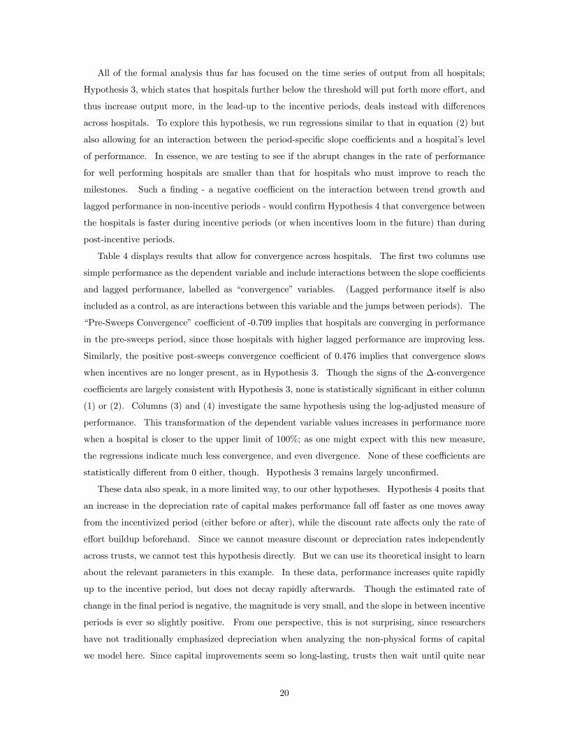
All of the formal analysis thus far has focused on the time series of output from all hospitals;

Hypothesis 3, which states that hospitals further below the threshold will put forth more effort, and

thus increase output more, in the lead-up to the incentive periods, deals instead with differences

across hospitals. To explore this hypothesis, we run regressions similar to that in equation (2) but

also allowing for an interaction between the period-specific slope coefficients and a hospital’s level

of performance. In essence, we are testing to see if the abrupt changes in the rate of performance

for well performing hospitals are smaller than that for hospitals who must improve to reach the

milestones. Such a finding - a negative coefficient on the interaction between trend growth and

lagged performance in non-incentive periods - would confirm Hypothesis 4 that convergence between

the hospitals is faster during incentive periods (or when incentives loom in the future) than during

post-incentive periods.

Table 4 displays results that allow for convergence across hospitals. The first two columns use

simple performance as the dependent variable and include interactions between the slope coefficients

and lagged performance, labelled as “convergence” variables. (Lagged performance itself is also

included as a control, as are interactions between this variable and the jumps between periods). The

“Pre-Sweeps Convergence” coefficient of -0.709 implies that hospitals are converging in performance

in the pre-sweeps period, since those hospitals with higher lagged performance are improving less.

Similarly, the positive post-sweeps convergence coefficient of 0.476 implies that convergence slows

when incentives are no longer present, as in Hypothesis 3. Though the signs of the ∆-convergence

coefficients are largely consistent with Hypothesis 3, none is statistically significant in either column

(1) or (2). Columns (3) and (4) investigate the same hypothesis using the log-adjusted measure of

performance. This transformation of the dependent variable values increases in performance more

when a hospital is closer to the upper limit of 100%; as one might expect with this new measure,

the regressions indicate much less convergence, and even divergence. None of these coefficients are

statistically different from 0 either, though. Hypothesis 3 remains largely unconfirmed.

These data also speak, in a more limited way, to our other hypotheses. Hypothesis 4 posits that

an increase in the depreciation rate of capital makes performance fall off faster as one moves away

from the incentivized period (either before or after), while the discount rate affects only the rate of

effort buildup beforehand. Since we cannot measure discount or depreciation rates independently

across trusts, we cannot test this hypothesis directly. But we can use its theoretical insight to learn

about the relevant parameters in this example. In these data, performance increases quite rapidly

up to the incentive period, but does not decay rapidly afterwards. Though the estimated rate of

change in the final period is negative, the magnitude is very small, and the slope in between incentive

periods is ever so slightly positive. From one perspective, this is not surprising, since researchers

have not traditionally emphasized depreciation when analyzing the non-physical forms of capital

we model here. Since capital improvements seem so long-lasting, trusts then wait until quite near

20

to the sweeps week to begin boosting performance, perhaps leaving high-return investments on the

table. This phenomenon could be the result of a high discount rate or of high fixed costs to exerting

positive effort.

The data are also consistent with Hypothesis 5, which predicts that the drop in output after

a prolonged incentive period will be less pronounced than that after a short one. We only have

two incentive periods, and thus we cannot make serious statistical inference about the validity of

this hypothesis, but the drop in output after the sweeps week is significantly greater than the drop

following the cash period in every specification. One potential alternative explanation for this

finding is that the government continued to closely monitor hospitals performing poorly following

the cash incentive, while they did not do so as intensely following the sweeps week. There is some

anecdotal evidence that this was the case. In any case, this hypothesis awaits more thorough testing.

We can do even less to test Hypothesis 6 within our data, as the level of intrinsic and basic

compensation is the same throughout our example. Workers in the A&E departments in these

hospitals are likely to have a high degree of intrinsic motivation, though; thus, our finding that

output does not fall much following the incentive periods is consistent with this prediction of our

model. We hope that future work will evaluate this model across a greater range of settings to

substantiate or qualify the suggestive evidence here.

5 Assessing Classical Effort Substitution and Gaming

The regressions in Table 3 formally confirm what Figure 2 depict: both the Sweeps Week and the

cash incentives led to lasting gains in performance. One potentially powerful alternative hypothesis,

though, is that hospitals simply reallocated production towards dimensions rewarded by the incen-

tives. As discussed in Section 2.3, hospitals facing convex costly adjustment along its production

possibilities frontier would produce a pattern of decreasing waiting times similar to that seen in the

results above, but the response to the incentives would not be “investment” in any real sense but

instead non-reversed effort substitution (akin to the result of policy persistence in Coate and Morris

(1999)). Though the inertial nature of the performance increases is interesting theoretically, the

lessons for public policy would be very different if these gains resulted from such institutionalized

effort substitution rather than true improvements in the quality of care. And since overall perfor-

mance may be difficult to quantify appropriately in this setting, agents have ample room to "game"

the system (see, for instance, Dixit 1996). This section investigates these possibilities by examining

changes in other output measures that were not incentivized.

21

5.1 Data and Summary Statistics

In addition to our primary series, we also have a number of alternative measures of quality of care,

albeit collected only every quarter, extending from the fourth quarter of 2002 through 2005. Our

non-incentivized measure of quality is the distribution of patient waiting times within one-hour bins

up to four hours. Most obviously, the four-hour cutoff gives A&Es an incentive to reduce the longest

waits by increasing the shortest waits. Since wait time in an emergency room is often determined

by the severity of a patient’s ailment, this redistribution would entail an increase in wait times for

more serious patients in exchange for a decrease for less serious patients. Unless the marginal cost

to patients of waiting is rapidly increasing, such a shift, all else equal, would lower the quality of

care, especially when serious patients have life-threatening conditions requiring rapid attention.

We also have data tracking the number of patients that return to the A&E department within a

short time after a related first visit. This statistic should give us another crude measure of quality,

since most of the return visits are in response to ineffective treatments.

Another more institution-specific method for artificially boosting the measured statistic is to

admit extra patients to inpatient wards. When patients requiring serious treatment come through

the A&E, they clearly cannot be fully treated within four hours, so the target specifies that they

must be admitted to inpatient wards (where further treatment will take place) within four hours.

Therefore, faced with the prospect that a patient might break the four-hour target, hospitals have

an incentive to admit that patient to the hospital rather than treat them in the A&E department;

such an unnecessary diversion is costly because the standard of care in inpatient units is higher, and

because free beds in the inpatient wards are often in short supply. Our data record the number of

patients admitted to the hospital in each quarter.19

Outright falsification is the most blatant channel available to trusts to avoid real reform. This

possibility concerned the officials administering these incentives as well. To combat this possibility,

the Department of Health conducted regular audits on the record-keeping in each trust. Though

the audits reveal a non-trivial error rate in the paperwork of 11%, mistakes were overwhelmingly

of a administrative nature. The audits revealed a few instances of errors in time records and no

evidence of systematic administrative fraud (Department of Health, 2005b).20

We first look at the distribution of waiting times within hospitals by quarter. The data sort

patient visits into hour-sized buckets up to four hours, as well as labelling breaches. If hospitals

are “gaming” the system in this way, then the fraction of patients in both short-wait and long-wait

19During the period covered by our data, many hospitals also introduced “clinical observation wards,” which wereinpatient facilities with lower standards than those in traditional hospital room (but higher than A&E departments),for A&E patients requiring tests that would take more than four hours. Patients admitted into these wards withinfour hours were considered to have met the four-hour target. However, such patients were coded as having beenadmitted to standard inpatient wards; thus, the extent that hospitals used these new wards to meet the standards isreflected in the inpatient admission figures.20 In Friedman and Kelman (2007b), we present other empirical tests of effort substitution and gaming, along with

a larger discussion of these issues.

22

bins should decrease over time. Figure 5A displays the distribution of patients across these buckets

in four distinct periods, each roughly one year apart. These periods occur before the sweeps week,

after the sweeps week, during the cash incentive, and after the cash incentive, respectively. The

procession of four bars within each cluster represents the fraction of patients within in given one-hour

bin during each of four time periods. Though the fraction of breaches shrink over time, the fraction

of patients in each lower bin grows, suggesting that hospitals are actually becoming more efficient.

Figure 5B represents these data in a slightly different way. The cumulative distribution of

patient waiting times is displayed vertically for any given quarter; as the height of each colored bar

changed, we can follow the cumulative distribution function evolving over time. This chart shows

that the distribution of patient waiting times in later periods nearly always first-order stochastically

dominates the distribution in any earlier period. This distribution shifts slightly up in the last

quarter plotted, mirroring the slight increase in breaches during this period shown in Figure 2. But

overall, hospitals do not appear to be sacrificing shorter stays to reach the milestone. We further

investigate this hypothesis in the regressions below using the fraction of patients waiting fewer than

two hours as a representative statistic for the size of the left tail of the wait time distribution.

Though the data only come in hour-sized bins, we can also calculate an approximation to the

mean waiting time for patients within a given trust and quarter. To do so, we assume that patients

in the 0 to 1 hour bucket, on average, waited 30 minutes, and so on upwards. Figure 6 displays the

evolution of this estimated mean waiting time using three different assumptions about the average

waiting time for those patients not treated within four hours. Even in the most conservative

specification, in which we assume that such patients were treated in an average of only four hours,

“mean” wait times improve by nearly 40 minutes, or more than 25%, over the sample period. The

changes are even starker for more realistic assumptions about the average waiting time for breached

patients. Figure 7 plots the distribution of mean waiting times across hospitals assuming a 5 hour

average for extreme waiting times. As with the measured statistic, the distribution converges over

time, and the convergence is once again most rapid in the periods with announced incentives. The

slight decrease in performance appears in the final quarter in Figure 6 as well. We further investigate

this calculation of “mean” effort in the regressions below.

Table 5 presents summary statistics for the four alternative measures of quality of care. As

shown above, the “mean” wait time decreases over time, while the percent of patients treated within

two hours increases. The fraction of patients who come into the A&E on a follow-up visit falls a bit

over our sample period; the percent of patients admitted to the general hospital increases slightly.

23

5.2 Results

To test for effort substitution, we estimate regressions of the general form

zht = α+ βyht + νh + ϕt + εht (3)

where zht represents a non-incentivized measure of performance, yht is the fraction of patients treated

in under four hours, νt and ϕh are quarter- and hospital-specific fixed effects, for hospital h in quarter

t. We also replace yht with ∆yht = yht− yh,t−1 in some specifications, and we experiment with the

alternatively scaled measure of effort yt, as discussed above. In this specification, the parameter

β estimates the extent to which increases in incentivized performance are associated with changes

in in the alternative performance measures; since our measures of alternative performance are bad,

an estimate of β > 0 implies that increases in targeted performance yht are associated with reduced

performance elsewhere, the telltale sign of effort substitution. If, on the other hand, β < 0, then

alternative performance and incentivized performance covary positively, a finding inconsistent with

hospitals substituting effort from one output to another to achieve the targets.21

Before presenting the results, it is useful to discuss two potential biases. First, there may be

reverse causality from the alternative measures of performance back onto the measured statistic. For

instance, suppose that different forms of effort are substitutes, as is the typical the case. Then if a

trust were to exogenously reduce the effort directed towards preventing follow-up visits, it would be

natural to increase the effort directed to reducing wait times below four hours. Such forces would

bias the coefficient of interest upwards in our framework, since we would be spuriously attributing

the rise in follow-up visits to the decrease in % of patients waiting more than four hours. Of course,

this is a bias in favor of each of the hypotheses; since we fail to confirm each one, and in many

cases find significant results in the “wrong” direction, such a bias should not impact our results.

In order for this simultaneity bias to confound our results, different forms of effort would need to

be complementary to the agent. But such a setup would itself rule out effort substitution, which

requires that effort towards different tasks be substitutes for the agent. Thus, we do not believe that

reverse causality is a problem here.

Another potential bias stems from correlated omitted variables. For instance, suppose that the

average severity of illness varies from week to week. This omitted variable would both increase

the percent of patients treated within four hours and increase a number of our alternative quality

measures, such as the death rate, producing a bias in our favor. In order to investigate this potential

21 So that lower measures of z are always better, we use the fraction of patients treated in more than two hours asour fourth statistic.

24

bias, we also run regressions using the specification

zht = α+ βyht + γyht ∗ It + νh + ϕt + εht (4)

where It is a dummy variable equal to one in the pre-sweeps or the cash incentive periods - that

is, in those periods where present or future incentives loomed. The parameter γ estimates effort

substitution by looking at the differential response rate to increases in the measured statistic be-

tween incentivized and non-incentivized periods; if we estimate γ > 0, there is evidence of effort

substitution. As before, we cluster standard errors by trust.

Table 6 reports results from this set of 32 regressions; there are 4 dependent variables (zht), 4

versions of the measured statistic (yht), and 2 specifications (those in equations (3) and (4)). A

vertical column displays the four regressions that share a dependent variable and a specification.

For instance, β = −0.050 when the dependent variable is “% Waiting > 2 Hours,” the independent

variable is the log-scaled version of the measured performance (yht), and the specification is that in

equation (3).

In general, statistically significant coefficients appear in the regressions using “mean” wait time

and the sub-two hour wait share as the dependent variable. But the increases in the incentivized

task here seem primarily to help these alternative measures, contrary to the effect predicted by effort

substitution. For instance, seven of eight of the statistically significant coefficients in the regressions

using “mean” wait time are negative, so that, as fewer patients wait more than four hours, mean

wait time decreases.22 Similarly, most of the significant coefficients in regressions using the sub-two

hour fraction are positive.

There are a few significant coefficients that go in the other (bad) direction, such as in the second

panel of columns (6) and (7). For instance, relative to a similar move in periods without incentives,

increasing performance by 1 percentage point increases the fraction of patients waiting more that

two hours by 0.275 percentage points. This effect is less than 2.5% of one standard deviation of

this variable, though. Similarly, a one percentage point increase in performance increases mean

wait time by 0.01 hours more in incentive periods than in other periods. The significant coefficients

in regressions using follow-up visits are even smaller in economic magnitude. In another paper,

we expand these estimates by looking at these measures over more time, as well as adding death

rates and orthopaedic surgery waiting times as alternative measures of output; these additional

results reinforce the findings here; there is no compelling evidence of any effort substitution. We

also present IV estimates, in which we instrument for performance with the timing of the incentive

period, that further reject effort substitution or reallocation as an alternative explanation.23

22This result is robust to instead making the extremely conservative assumption that breached patients wait onlyfour hours, on average.23 See Friedman and Kelman (2008).

25

6 Discussion

While the private sector has traditionally turned to performance-based incentives to manage a

workforce, governments have only recently begun to do so for their many employees. For example,

the US government implemented performance-related pay for job-counselors and managers in the

Job Training and Partnership Act in 1983. New Zealand’s Reserve Bank Act of 1989 details a

scheme of incentive-based compensation for the central bank’s Chairman. Most recently, school

systems in Houston and Denver adopted government-funded incentive pay for teachers.

The success of public sector incentive schemes has been mixed; indeed, theory suggests that

the public sector may be especially susceptible to many of the familiar pitfalls of formal incentives.

Standard political economy problems may generate crude and inefficient contracts, while the multiple

objectives often involved in public sector activities make performance difficult to quantify and thus

give agents ample room to “game” the system. Due to the multifaceted nature of public services,

Holmström and Milgrom (1991) and Baker (1992) suggest that the optimal contract may avoid

incentives entirely. Organizations overseeing service provision in the public sector may be more

inefficient than parallel structures in the private sector, perhaps even optimally so (Prendergast,

2003), but the monitoring required for proper incentives may suffer as a result.

But if effort has a positive impact on the capital stock, as in these results, even weak incentives

may be able to produce greater effects than typically imagined. Investment effects would also be

expected to reduce problems with effort substitution across periods and tasks. Performance-based

incentives may thus have substantially greater scope in the public sector than previously believed.

That public sector employees tend to be intrinsically motivated, which they may be endogenously

(Prendergast, 2007), makes it more likely that gains from increases in human or organizational

capital in government should last for some time; in the public management literature, this is often

referred to as “public service motivation” (Perry and Wise, 1990, and Crewson, 1997). However, if

incentives were to encourage public sector employees to develop experience in unproductive activities,

the long-term efforts predicted by our model might make the situation far worse.

Another factor tending towards improvements through investments in the public sector is a

political constraint on government statements. In many cases, it is far less politically accept-

able for governments to recommend that public sector employees simply “try harder” to improve

performance; instead, governments are more likely to suggest various procedural or managerial im-

provements. One can see this emphasis in general government communications to employees in the

context of increasing performance; the British government focused on various process improvements

(such as a reform of triage procedures) in the lead-up to the incentives studied here, and the U.S.

government has focused almost exclusively on similar changes when dealing with schools (as in the

reforms following the No Child Left Behind reforms). If agents find it easiest to “look under the

lamp post” and follow government directions, the effects of incentives through investment we study

26

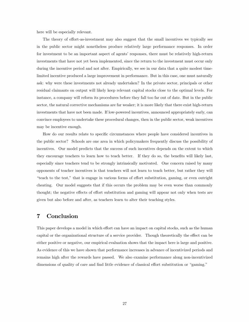
here will be especially relevant.

The theory of effort-as-investment may also suggest that the small incentives we typically see

in the public sector might nonetheless produce relatively large performance responses. In order

for investment to be an important aspect of agents’ responses, there must be relatively high-return

investments that have not yet been implemented, since the return to the investment must occur only

during the incentive period and not after. Empirically, we see in our data that a quite modest time-

limited incentive produced a large improvement in performance. But in this case, one must naturally

ask: why were these investments not already undertaken? In the private sector, principals or other

residual claimants on output will likely keep relevant capital stocks close to the optimal levels. For

instance, a company will reform its procedures before they fall too far out of date. But in the public

sector, the natural corrective mechanisms are far weaker; it is more likely that there exist high-return

investments that have not been made. If low-powered incentives, announced appropriately early, can

convince employees to undertake these procedural changes, then in the public sector, weak incentives

may be incentive enough.

How do our results relate to specific circumstances where people have considered incentives in

the public sector? Schools are one area in which policymakers frequently discuss the possibility of

incentives. Our model predicts that the success of such incentives depends on the extent to which

they encourage teachers to learn how to teach better. If they do so, the benefits will likely last,

especially since teachers tend to be strongly intrinsically motivated. One concern raised by many

opponents of teacher incentives is that teachers will not learn to teach better, but rather they will

“teach to the test,” that is engage in various forms of effort substitution, gaming, or even outright

cheating. Our model suggests that if this occurs the problem may be even worse than commonly

thought; the negative effects of effort substitution and gaming will appear not only when tests are

given but also before and after, as teachers learn to alter their teaching styles.

7 Conclusion

This paper develops a model in which effort can have an impact on capital stocks, such as the human

capital or the organizational structure of a service provider. Though theoretically the effect can be

either positive or negative, our empirical evaluation shows that the impact here is large and positive.

As evidence of this we have shown that performance increases in advance of incentivized periods and

remains high after the rewards have passed. We also examine performance along non-incentivized

dimensions of quality of care and find little evidence of classical effort substitution or “gaming.”

27

8 Bibliography

1. Argote, Linda (1999). Organizational Learning: Creating, Retaining and Transferring Knowl-

edge. New York: Springer.

2. Arrow, Kenneth. (1962). “The Economic Implications of Learning by Doing.” Review of

Economic Studies, Vol 29(3), pp. 155-73.

3. Baker, George. (1992). “Incentive Contracts and Performance Measurement.” Journal of

Political Economics, Vol 100, pp. 598-614.

4. Bandiera, Oriana, Iwan Barankay, and Imran Rasul (2005). “Social Preferences and the

Response to Incentives: Evidence from Personnel Data.” Quarterly Journal of Economics,

Vol 120, p. 917-62.

5. Barnard, Chester I. (1938). The Functions of the Executive. Cambridge, MA: Harvard

University Press.

6. British Broadcasting Corporation. (2006). “Trust Plans Hospital Takeover.” Available at

http://news.bbc.co.uk/1/hi/england/west_midlands/5399130.stm

7. Chart, Elizabeth. (1996). “The Performance Measurement Agenda in the NHS.” University

of Southampton Unpublished Masters Thesis.

8. Crewson, Philip E. (1997). “Public Service Motivation; Building Empirical Evidence of

Incidence and Effect.” Journal of Public Adminstration Research and Theory, Vol. 4, pp.

499-518.

9. Coate, Steven, and Steven Morris. (1999). “Policy Persistence.” American Economic Review,

Vol 89(5), p. 1327-36.

10. Deci, Edward. (1971). “Effects of Externally Mediated Rewards on Intrinsic Motivation.”

Journal of Personality and Social Psychology, Vol 18, p. 105-15.

11. Department of Health. (2000). “The NHS Plan: A Plan for Investment, A Plan for Reform.”

Available at http://www.nhsia.nhs.uk/nhsplan/nhsplan.htm

12. Department of Health. (2001). “NHS Reform Bill Published.” Available at http://www.dh.gov.uk/PublicationandSt

13. Department of Health. (2005a). “Department Report 2005.” Available at http://www.dh.gov.uk/assetRoot/04/11/

14. Department of Health. (2005b). “A&E Update, 10/12.” Section 5.1.1.

15. Dixit, Avinash K. (1996). The Making of Economic Policy: A Transaction-Cost Politics

Perspective. Cambridge, MA: MIT Press.

28

16. Dixit, Avinash K. (2002). “Incentives and Organizations in the Public Sector; An Interpretive

Review.” Journal of Human Resources, Vol 37(4), pp. 696-727.

17. Dranove, David, Daniel Kessler, Mark McCellan, and Mark Satterthwaite. (2003). “Is More

Information Better? The Effects of “Report Cards” on Healthcare Providers.” Journal of

Political Economy, Vol 111(3), pp. 555-88.

18. Friedman, John and Steve Kelman. (2008) “Performance Improvement and Performance

Disfunction: An Empirical Examination of Distortionary Impacts of the Emergency Room

Wait-Time Target in the English National Health Service.” Harvard UniversityWorking Paper.

19. Gneezy, Uri and Aldo Rustichini. (2000). “Pay Enough or Dont Pay At All.” Quarterly

Journal of Economics, Vol 115, p. 791-811.

20. Harris, Milton, and Bengt Holmström. (1982). “A Theory of Wage Dynamics.” Review of

Economic Studies, Vol 49, p. 315-53.

21. Hauck, Katharina, and Andrew Street. (2007). “Do Targets Matter? A Comparison of

English and Welsh National Health Priorities.” Health Economics. Vol. 16, pp. 275-290.

22. Healy, Paul M. (1985). “The effect of Bonus Schemes on Accounting Schemes.” Journal of

Accounting and Economics, Vol. 7, pp., 85-107.

23. Heckman, James, Carolyn Heinrich and Jeffrey Smith (1997). “Assessing the Performance

of Performance Standards in Public Bureaucracies.” American Economic Review, Vol 87, p.

389-95.

24. Holmström, Bengt, and Paul Milgrom. (1991). “Multitask Principal-Agent Analyses: Incen-

tive Contract, Asset Ownership, and Job Design.” Journal of Law, Economics, and Organi-

zations, Vol 7, pp.24-53.

25. Kelman, Steve. (2006). “Improving Service Delivery Performance in the United Kingdom:

Organization Theory Perspective on Central Intervention Strategies.” Journal of Comparative

Policy Analysis, Vol 8(4), p. 393-419.

26. McNichols, Maureen F. (2000). “Research Design Issues in Earnings Management Studies.”

Journal of Accounting and Public Policy, Vol 19, pp. 313-45.

27. Nelson, Richard and Sidney G. Winter. (1982) An Evolutionary Theory of Economics Change.

Cambridge, MA: Belknap Press of Harvard University Press.

28. Oyer, Paul (1998). “Fiscal Year Ends and Nonlinear Incentive Contracts: The Effects on

Business Seasonality.” Quarterly Journal of Economics, Vol 113, pp. 149-85.

29

29. Perry, James L. and Lois R. Wise. (1990). “The Motivational Bases of Public Service.”

Public Administration Review, Vol 50, pp. 367-73.

30. Propper, Carol, Matt Sutton, Carolyn Whitnall, and Frank Windmeijer. (2008). “Did

’Target and Terror’ Reduce Waiting Times in England for Hospital Care?” B.E. Journal of

Economic Analysis and Policy, Vol 8: Iss. 2 (Contributions), Article 5.

31. Prendergast, Canice. (1999). “The Provision of Incentives in Firms.” Journal of Economic

Literature, Vol 3, pp. 7-63.

32. Prendergast, Canice. (2003). “The Limits of Bureaucratic Efficiency.” Journal of Political

Economy, Vol 111(5), pp. 929-58.

33. Prendergast, Canice. (2007). “The Motivation and Bias of Bureaucrats.” American Eco-

nomic Review, Vol. 97(1), pp. 180-96.

34. Rosenthal, Meredith, and Richard G. Frank. (2006). “What is the Empirical Basis for Paying

for Quality in Healthcare?” Medical Care Research and Review, Vol 63(2), pp. 135-57.

35. Schmenner, Roger. (1993). Production/Operations Management. Fifth Edition, Englewood

Cliffs: Prentice-Hall.

36. Stein, Jeremy. (1989). “Efficient Capital Markets, Inefficient Firms.” Quarterly Journal of

Economics, Vol 104(4), pp. 655-69.

37. Williamson, Oliver E. (1975). Markets and Hierarchies: Analysis and Antitrust Implications.

New York: The Free Press.

9 Appendix

Proof of Proposition 1. The agent solves the problem

max{ht,lt}∞t=0

E∞Xt=0

βt [vt − c (ht, lt)] ,

where vt = 0 for t 6= T , and vT = wyT +W ∗I {yt > χ}. Substituting in for the production function,the capital stock, and the expected reward, we can rewrite the program as

max{ht,lt}∞t=0

βT

"W

Ã1− F

Ãχ− γhT − (1− δ) K −

T−1Xt=0

δT−t [φlt + λht]

!!+ w

ÃγhT + (1− δ) K +

T−1Xt=0

δT−t [φlt + λht]

!#

The program seeks to maximize a concave function over a convex set, and so the first order conditions

are necessary and sufficient conditions for maximization so long as the choice variables are positive.

30

Differentiation yields the set of FOCs⎧⎨⎩ lt : βTφδT−t [Wf (χ−EyT ) + w] = βtcl

ht : βTλδT−t [Wf (χ−EyT ) + w] = βtch

⎫⎬⎭ for t < T

⎧⎨⎩ lt : 0 = βT c0 (ht + lt)

ht : βT γ [Wf (χ−EyT ) + w] = βT c0 (ht + lt)

⎫⎬⎭ for t = T

⎧⎨⎩ lt : 0 = βtcl

ht : 0 = βtch

⎫⎬⎭ for t > T.

It is clear that, for all parameter values, h∗t = l∗t = 0 for t > T . λ < 0 has no impact on effect levels,

in this simple setup.

When φ > 0, it is clear that ht = 0 for t < T . Defining z (·) = [cl (0, l)]−1 = [ch (h, 0)]−1 andtaking ratios implies that

lthT

=z³φ (βδ)

T−t[Wf (χ−EyT ) + w]

´z (γ [Wf (χ−EyT ) + w])

. (5)

Note that z (0, 0) = 0. Thus, we know that

φ (βδ)T−t [Wf (χ−EyT ) + w] > 0 ⇐⇒ et > 0

and therefore that φ > 0 implies lt = 0. When λ < 0 = φ, or [Wf (χ−EyT ) + w] = 0 imply

eT = 0.

We also know that z (·) is an increasing function, and therefore that, when φ [Wf (χ−EyT ) + w] >

0, that lt < lt+1 < hT for t < T .

Proof of Proposition 2. From equation (5) above, we know that, when φ > 0, then

lt = z³φ (βδ)T−t [Wf (χ−EyT ) + w]

´hT = z (γ [Wf (χ−EyT ) + w])

for t < T

for t = T.

Thus, without needing to calculate EyT explicitly, we can derive the time series ratios of output.

We know that, for t < T ,

Eyt =t−1Xs=0

δt−sφhs + K =t−1Xs=0

φδt−sz³φ (βδ)

T−s[Wf (χ−EyT ) + w]

´+ K.

31

The ratio between output in different periods will then satisfy

Eyt−1Eyt

=

Pt−2s=0 φδ

t−s−1z³φ (βδ)

T−s £Wf

¡χ− K −EyT

¢+ w

¤´Pt−1

s=0 φδt−sz

³φ (βδ)T−s

£Wf

¡χ− K −EyT

¢+ w

¤´ .

Since z0 > 0, then for all s

z³φ (βδ)

T−s−1 £Wf

¡χ− K −EyT

¢+ w

¤´> z

³φ (βδ)

T−s £Wf

¡χ− K −EyT

¢+ w

¤´the set of terms in the denominator pairwise deminates those in the denominator, the extra positive

term in the denominator (φδtz³φ (βδ)

T−s £Wf

¡χ− K −EyT

¢+ w

¤´remains unpaired) notwith-

standing. Therefore,

Eyt > Eyt−1 ∀t ≤ T.

For t > T , we know that

Eyt = φδt−TTXs=0

δT−ses = φδt−T"T−1Xs=0

δT−sz³φ (βδ)T−s

£Wf

¡χ− K −EyT

¢+ w

¤´+ z

¡γ£Wf

¡χ− K −EyT

¢+ w

¤¢#

and thus thatEyt+1 − K

Eyt − K= δ (6)

Beginning at time t = T + 1, output remains positive but decays exponentially as the capital stock

depreciates back to K.

When λ < 0 = φ, then EyT = hT + K = z¡γ£Wf

¡χ− K −EyT

¢+ w

¤¢as above. But instead

of decaying down to 0 when t > T , output will drop to

EyT+1 = δλhT < 0,

after which point the ratio Eyt+1−KEyt−K = δ from above will obtain, with all Eyt < K where t > T .

Proof of Proposition 3. The level of effort depends on the marginal distribution of εt around

the value χ− K −EyT . We know that

EyT =T−1Xs=0

φδT−sz³φ (βδ)

T−s £Wf

¡χ− K −EyT

¢+ w

¤´+ γz

¡γ£Wf

¡χ− K −EyT

¢+ w

¤¢.

Since z0 > 0 and f 0 > 0 by assumption, implicitly differentiating this expression implies that

∂EyT∂K

=

PT−1s=0 Wφ2

¡βδ2

¢T−sz0³φ (βδ)

T−s[Wf + w]

´f 0 + γ2Wz0 (γ [Wf + w]) f 0PT−1

s=0 Wφ2¡βδ2

¢T−sz0³φ (βδ)

T−s[Wf + w]

´f 0 + γ2Wz0 (γ [Wf + w]) f 0 + 1

∈ (0, 1)

32

It is a parallel calculation that, given this derivative, ∂Eyt∂K

for which t 6= T .

Proof of Corollary 1. If there is a fixed cost ψ to acting in each period, then, if agents act, they

will act as they did before, since ψ does not alter the incentives on the margin. However, the agent

will only act if

∆EyT (lt)£Wf

¡χ− K −EyT

¢+ w

¤> ψ.

We know from the production function and equation (5) that

∆EyT (lt) = φδT−tz³φ (βδ)

T−t £Wf

¡χ− K −EyT

¢+ w

¤´,

which is clearly a monotonically increasing function in t. Thus there exists a unique τ such that

∆EyT (lτ−1)£Wf

¡χ− K −EyT

¢+ w

¤< ψ < ∆EyT (lτ )

£Wf

¡χ− K −EyT

¢+ w

¤.

33

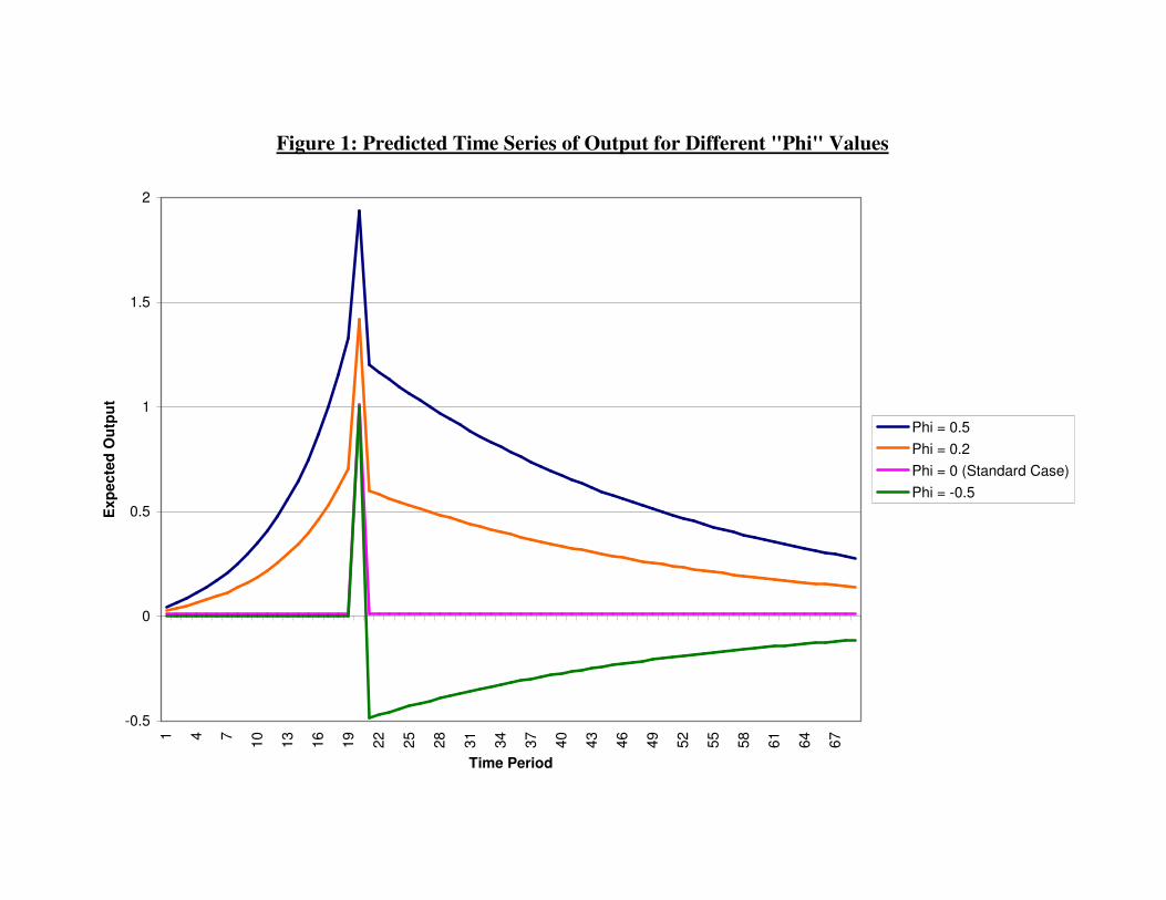
Figure 1: Predicted Time Series of Output for Different "Phi" Values

-0.5

0

0.5

1

1.5

2

1 4 7 10 13 16 19 22 25 28 31 34 37 40 43 46 49 52 55 58 61 64 67

Time Period

Exp

ecte

d O

utpu

t

Phi = 0.5Phi = 0.2Phi = 0 (Standard Case)Phi = -0.5

Figure 2: Mean Hospital Performance over Time

75%

80%

85%

90%

95%

100%

4/7/20

02

7/7/20

0210

/7/20

02

1/7/20

03

4/7/20

03

7/7/20

0310

/7/20

03

1/7/20

04

4/7/20

04

7/7/20

0410

/7/20

04

1/7/20

05

4/7/20

05

7/7/20

0510

/7/20

05

1/7/20

06

4/7/20

06

7/7/20

06

Type 1 Patients All Patients

INCENTIVES

"INTERIMMILESTONE"

ANNOUNCEMENT

ANNOUNCEMENT

Figure 3: Quantiles of Hospital Performance over Time

0.5

0.55

0.6

0.65

0.7

0.75

0.8

0.85

0.9

0.95

1

4/1/20

02

7/1/20

02

10/1/

2002

1/1/20

03

4/1/20

03

7/1/20

03

10/1/

2003

1/1/20

04

4/1/20

04

7/1/20

04

10/1/

2004

1/1/20

05

4/1/20

05

7/1/20

05

10/1/

2005

1/1/20

06

4/1/20

06

7/1/20

06

90th Percentile 75th Percentile 50th Percentile 25th Percentile 10th Percentile

Figure 4: Hospital Performance over Time, by Initial Quality

0.6

0.65

0.7

0.75

0.8

0.85

0.9

0.95

1

1/5/

2003

3/5/

2003

5/5/

2003

7/5/

2003

9/5/

2003

11/5

/200

3

1/5/

2004

3/5/

2004

5/5/

2004

7/5/

2004

9/5/

2004

11/5

/200

4

1/5/

2005

3/5/

2005

5/5/

2005

7/5/

2005

9/5/

2005

11/5

/200

5

1/5/

2006

3/5/

2006

5/5/

2006

Low Quintile Mid-Low Quintile Mid Quintile Mid-High Quintile High Quintile

Table 5A: Distribution of Waiting Times

0

0.05

0.1

0.15

0.2

0.25

0.3

0.35

0 to 1 1 to 2 2 to 3 3 to 4 Breach

Hours

2003, Q32004, Q22005, Q22006, Q2

Table 5B: Evolution of the Waiting Time Distribution

0

0.1

0.2

0.3

0.4

0.5

0.6

0.7

0.8

0.9

1

2003.3 2003.4 2004.1 2004.2 2004.3 2004.4 2005.1 2005.2 2005.3 2005.4 2006.1 2006.2 2006.3

Fiscal Period

Cum

ulat

ive

% o

f Pat

ient

s

BreachesWaits 3 to 4 HoursWaits 2 to 3 HoursWaits 1 to 2 HoursWaits < 1 Hour

Figure 6: "Mean" Waiting Times

1

1.5

2

2.5

3

3.5

2003.3 2003.4 2004.1 2004.2 2004.3 2004.4 2005.1 2005.2 2005.3 2005.4 2006.1 2006.2 2006.3

Hou

rs

E[Wait|Breach] = 4 Hours E[Wait|Breach] = 5 Hours E[Wait|Breach] = 6 Hours

Figure 7: Distribution of "Mean" Waiting Time Across Hospitals

1

1.5

2

2.5

3

3.5

2003.3 2003.4 2004.1 2004.2 2004.3 2004.4 2005.1 2005.2 2005.3 2005.4 2006.1 2006.2 2006.3

Time

Hou

rs

10th Percentile25th Percentile50th Percentile75th Percentile90th Percentile

Table 1: Threshold Clearance Rates

Threshold Rate

94% 52.6%95% 43.5%96% 42.2%97% 42.9%98% 27.9%

Met All Thresholds 9.1%Met No Thresholds 20.8%

Table 2: Performance Summary Statistics

Panel A: Entire Samplew/i Trust

Variable Mean Std. Dev. RMSE N

Performance: Type 1 Patients 91.30% 9.52% 2.83% 35797

Performance: All Patients 96.51% 3.46% 1.59% 23870

Type 1 Attendances 1604 691 110 35797

Type 1 Breaches 139.7 172.3 47.2 35797

Panel B: Type 1 Performance, Period by Periodw/i Trust

Period Variable Mean Std. Dev. RMSE N

Performance 78.96% 12.58% 4.42% 6037Base Attendance 1491 656 123 6037

Breaches 325.4 255.6 70.1 6037

Performance 82.55% 8.93% 3.23% 1705Pre-"Sweeps" Attendance 1448 631 65 1705

Breaches 262.5 192.4 51.1 1705

Performance 93.01% 5.02% - 155"Sweeps" Week Attendance 1606 709 - 155

Breaches 114.4 95.6 - 155

Performance 88.34% 6.20% 3.21% 6355Middle Attendance 1564 668 98 6355

Breaches 188.7 137.1 53.3 6355

Performance 90.77% 5.02% 2.10% 1085Pre-Cash Attendance 1468 637 59 1085

Breaches 141.5 109.4 31.7 1085

Performance 95.01% 3.60% 2.40% 8680Cash Incentive Attendance 1625 691 104 8680

Breaches 85.9 82.3 42.0 8680

Performance 97.79% 2.00% 1.62% 11780Post Incentive Attendance 1702 718 123 11780

Breaches 40.0 42.9 30.7 11780

Table 3: Time Series Analysis of Performance

Dependent Variable:Explanatory Type 1 Performance -LOG(1-Performance) Variables: (1) (2) (3) (4) (5) (6)

"Sweeps Announcement" Jump -0.08 -0.28 -0.05 -5.31 -5.73* -5.37(0.40) (0.36) (0.38) (2.84) (2.61) (3.08)

"Sweeps Week" One-Time Jump 6.97** 6.97** 6.82** 78.5** 78.6** 89.0**(0.48) (0.48) (0.48) (5.53) (5.52) (6.81)

Post "Sweeps Week" Jump 1.68** 1.40** 0.76 15.6** 14.4** 7.39(0.41) (0.44) (0.47) (3.73) (3.98) (4.19)

"Cash Announcement" Jump 0.44 0.61 0.65* 3.83 3.61 5.04(0.32) (0.31) (0.31) (2.62) (3.67) (4.45)

"Cash Period" Jump 1.02** 0.56* 0.61* 4.67 8.47* 14.1*(0.26) (0.24) (0.26) (3.93) (3.54) (4.08)

Post-Cash Jump 0.53** 0.55* -0.51* 30.0** 13.08* -35.1**(0.13) (0.21) (0.22) (3.97) (5.44) (6.14)

Base Period Slope 0.01 - - -0.30* - -(0.02) (0.12)

"Sweeps Announcement" ΔSlope 0.57** 0.55** 0.46** 3.95** 3.97** 3.43**(0.07) (0.08) (0.08) (0.55) (0.59) (0.66)

Post-"Sweeps" ΔSlope -0.55** -0.52** -0.65** -3.53** -3.24** -4.71**(0.07) (0.09) (0.10) (0.58) (0.83) (0.88)

"Cash Announcement" ΔSlope 0.26** 0.31** 0.19* 3.41** 3.01** 1.65(0.06) (0.08) (0.08) (0.67) (1.04) (1.15)

"Cash Period" ΔSlope -0.20** -0.16* -0.36** -1.54* -2.05* -6.74**(0.05) (0.07) (0.08) (0.66) (0.82) (0.92)

Post-"Cash" ΔSlope -0.09** 0.08* -0.11* -2.12** 2.09* -8.04**(0.01) (0.03) (0.05) (0.13) (0.87) (0.96)

Smooth Cubic Spline in Time? no yes yes no yes yes

Trust Effects? yes yes yes yes yes yes

Seasonally Adjusted? no no yes no no yes

R-Squared 0.6711 0.6716 0.6721 0.7310 0.7347 0.7377N 35797 35797 35797 35797 35797 35797Statistical significance is denoted with the system: * 5%, ** 1%. Standard errors are clustered at the trustlevel. Smooth cubis spline in time is continuous in the first derivative, with two equalled spaced knot-points. Dependent variable has been multiplied by 100, and thus represents percentage points.

Table 4: Convergence Across Hospitals over Time

Dependent Variable:Explanatory Type 1 Performance -LOG(1-Performance) Variables: (1) (2) (3) (4)

Pre-Sweeps Slope 0.583** - 3.65** -(0.027) (0.27)

Pre-Sweeps Convergence -0.709* -0.709* 0.344 0.344(0.347) (0.347) (0.594) (0.598)

Post-"Sweeps" �Slope -0.553** -0.495** -3.52** -1.86**(0.027) (0.032) (0.28) (0.37)

"Cash Period" �Slope 0.069** 0.211** 1.95** 1.20**(0.004) (0.013) (0.06) (0.21)

Post-"Cash" �Slope -0.102** 0.038** -2.21** 0.14(0.002) (0.010) (0.05) (0.31)

Post-Sweeps, � Converg. 0.476 0.476 -0.557 -0.557(0.367) (0.366) (0.593) (0.598)

Cash Period, � Converg. 0.038 0.038 0.134 0.134(0.113) (0.108) (0.113) (0.114)

Post-Cash, � Converg. 0.314 0.314 0.132 0.132(0.108) (0.101) (0.090) (0.090)

Quintic in Time? no yes no yes

Trust Effects? yes yes yes yes

R-Squared 0.8499 0.8525 0.7857 0.7894N 29605 29605 29605 29605

Statistical significance is denoted with the system: * 5%, ** 1%. Standard errors areclustered at the trust level.

Table 5: Summary Statistics for Non-Incentivized Performance Measures

Panel A: Entire Sample

Variable Mean Std. Dev. N

% Patients Treated < 2 Hours 56.73% 10.92% 1979

"Mean" Patient Wait Time 2.02 0.37 1979

% Patients Admitted to Hospital 18.53% 5.37% 2008

% Patients on Return Visit 5.12% 3.53% 2002

Panel B: Type 1 Performance, Period by Period

Period Variable Mean Std. Dev. N

% Patients Treated < 2 Hours 49.27% 12.19% 288Pre-Sweeps "Mean" Patient Wait Time 2.41 0.45 288

% Patients Admitted to Hospital 18.17% 4.96% 471% Patients on Return Visit 6.40% 4.34% 471

% Patients Treated < 2 Hours 55.04% 11.04% 458Middle "Mean" Patient Wait Time 2.12 0.35 458

% Patients Admitted to Hospital 17.79% 5.20% 458% Patients on Return Visit 5.56% 3.40% 457

% Patients Treated < 2 Hours 57.61% 9.73% 154Cash Incentive "Mean" Patient Wait Time 2.01 0.29 154

% Patients Admitted to Hospital 19.40% 5.69% 154% Patients on Return Visit 5.02% 2.76% 149

% Patients Treated < 2 Hours 59.31% 9.56% 1079Post-Cash "Mean" Patient Wait Time 1.88 0.26 1079

% Patients Admitted to Hospital 18.94% 5.55% 925% Patients on Return Visit 4.26% 2.97% 925

Table 6: Testing for Classical Effort Substitution

Dependent Variable:Explanatory Follow Up Visits Hospital Admits % Waits > 2 Hours "Mean" Wait TimeVariables: (1) (2) (3) (4) (5) (6) (7) (8)

Performance 0.013 -0.018 -0.030 -0.046 -0.662** -0.659** -3.207** -3.186**(0.169) (0.037) (0.021) (0.032) (0.067) (0.088) (0.180) (0.236)

Performance*Incentives - 0.034 - 0.018 - -0.004 - -0.028(0.036) (0.026) (0.071) (0.202)

ΔPerformance -0.016 -0.046* 0.003 -0.018 -0.105 -0.345** -0.527** -1.369**(0.009) (0.022) (0.014) (0.034) (0.061) (0.070) (0.198) (0.196)

ΔPerformance*Incentives - 0.037 - 0.025 - 0.275** - 1.053**(0.023) (0.039) (0.085) (0.247)

Log Performance 0.003 0.000 -0.002 -0.001 -0.050** -0.044** -0.221** -0.184**(0.002) (0.003) (0.003) (0.002) (0.006) (0.007) (0.018) (0.020)

Log Performance - 0.004 - -0.001 - -0.012* - -0.067*Incentives (0.003) (0.002) (0.006) (0.018)

ΔLog Performance -0.001 -0.004** -0.002 0.000 -0.028** -0.029** -0.107** -0.102**(0.001) (0.001) (0.001) (0.002) (0.003) (0.004) (0.008) (0.012)

ΔLog Performance - 0.005** - -0.002 - 0.002 - -0.010*Incentives (0.002) (0.003) (0.006) (0.017)

Trust Effects? yes yes yes yes yes yes yes yes

Quarter Effects? yes yes yes yes yes yes yes yes

N 2002 / 1841 2008 / 1847 1979 /1979 1979 /1979Statistical significance is denoted with the system: * 5%, ** 1%. Standard errors are clustered at the trust level. The numberof observations records two sample sizes: that for the level regressions, and that for the difference regressions, respectively.The dependent variables, when percentages, are scaled to range from 0 to 100. Performance as an independent variable isscaled from 0 to 1.