Eindhoven University of Technology MASTER Chlamydomonas

Eindhoven University of Technology

MASTER

Chlamydomonas Reinhardtiifrom microscopic swimming to macroscopic rheology

Boesten, R.J.J.

Award date:2011

Link to publication

DisclaimerThis document contains a student thesis (bachelor's or master's), as authored by a student at Eindhoven University of Technology. Studenttheses are made available in the TU/e repository upon obtaining the required degree. The grade received is not published on the documentas presented in the repository. The required complexity or quality of research of student theses may vary by program, and the requiredminimum study period may vary in duration.

General rightsCopyright and moral rights for the publications made accessible in the public portal are retained by the authors and/or other copyright ownersand it is a condition of accessing publications that users recognise and abide by the legal requirements associated with these rights.

• Users may download and print one copy of any publication from the public portal for the purpose of private study or research. • You may not further distribute the material or use it for any profit-making activity or commercial gain

https://research.tue.nl/en/studentTheses/898463ba-8e8a-48d3-b32a-c08fdaea07c7

Chlamydomonas Reinhardtii:

from microscopic swimming to macroscopic rheology

R.J.J. Boesten June 9, 2011

Abstract

The unicellar green alga Chlamydomonas Reinhardtii has two flagella with which it performsa ’breaststroke’ like movement to propel itself. This alga is currently investigated for indus-trial purposes on the macroscale, and has recently drawn attention by physical experiments onthe microscale of a single organism. This thesis aims to give an insight in both the swimmingbehaviour of a single alga and the influence of swimming at the macroscopic properties of suspen-sions of many algae. The simple analytic three-point-force model and a qualitative analysis ofthe flagellar stroke reproduces the experimentally obtained flow fields of Guasto et al. [23]. Twonew derivations are presented for the effective viscosity of a dilute suspension of Chlamydomonascells. Both are in agreement with previous theoretical results. The effective viscosity dependson the average swimming direction of the algae. A literature study on the ordering of activesuspensions leads to the conclusion that swimming results in an increase of the viscosity forsmall shear rates, for higher shear rates it is undistinguishable compared to a passive suspension.

1

Contents

1 Introduction in the microswimmer world 4

2 General physics of microswimming 62.1 Hydrodynamics at low Reynolds number . . . . . . . . . . . . . . . . . . . . . . . 62.2 Scallop theorem . . . . . . . . . . . . . . . . . . . . . . . . . . . . . . . . . . . . . 92.3 Brownian motion, diffusion and random walks . . . . . . . . . . . . . . . . . . . . 92.4 Flagellar propulsion . . . . . . . . . . . . . . . . . . . . . . . . . . . . . . . . . . 102.5 Theoretical models . . . . . . . . . . . . . . . . . . . . . . . . . . . . . . . . . . . 13

3 The motion and induced flows of Chlamydomonas Reinhardtii 143.1 Introducing Chlamydomonas - history and characteristics . . . . . . . . . . . . . 143.2 The Chlamydomonas flagellum & motility modes . . . . . . . . . . . . . . . . . . 153.3 Basal body and flagellar synchronisation . . . . . . . . . . . . . . . . . . . . . . . 173.4 Experimental flows . . . . . . . . . . . . . . . . . . . . . . . . . . . . . . . . . . . 173.5 Three-point-force model . . . . . . . . . . . . . . . . . . . . . . . . . . . . . . . . 18

4 Rheology of a suspension of Chlamydomonas Reinhardtii 254.1 What is viscosity? . . . . . . . . . . . . . . . . . . . . . . . . . . . . . . . . . . . 254.2 Cone-plate rheometer and simple shear flow . . . . . . . . . . . . . . . . . . . . . 264.3 Rheology of dilute suspensions of passive particles . . . . . . . . . . . . . . . . . 27

4.3.1 Spherical particles . . . . . . . . . . . . . . . . . . . . . . . . . . . . . . . 274.3.2 Gyrotactic particles . . . . . . . . . . . . . . . . . . . . . . . . . . . . . . 304.3.3 Ellipsoidal particles . . . . . . . . . . . . . . . . . . . . . . . . . . . . . . 32

4.4 Rheology of dilute suspensions of swimming Chlamydomonas . . . . . . . . . . . 354.4.1 Three-point-force model . . . . . . . . . . . . . . . . . . . . . . . . . . . . 354.4.2 Incorporating flagella . . . . . . . . . . . . . . . . . . . . . . . . . . . . . 38

4.5 Statistical description . . . . . . . . . . . . . . . . . . . . . . . . . . . . . . . . . 394.6 Rheological experiments on Chlamydomonas . . . . . . . . . . . . . . . . . . . . 424.7 Numerical modelling of swimmer suspensions . . . . . . . . . . . . . . . . . . . . 444.8 Rheology of non-dilute suspensions of Chlamydomonas . . . . . . . . . . . . . . . 44

5 Conclusion & discussion 46

A Acknowledgment 48

B Technology assessment 49

C Hydrodynamics 50

2

D Three-point-force model 53

E Stress tensor 56

F Squirmer: a theoretical swimmer 58

G Einstein derivation of the effective viscosity of a suspension of Chlamydomonas 60

H Volume average effective viscosity of a suspension of Chlamydomonas 63

3

Chapter 1

Introduction in themicroswimmer world

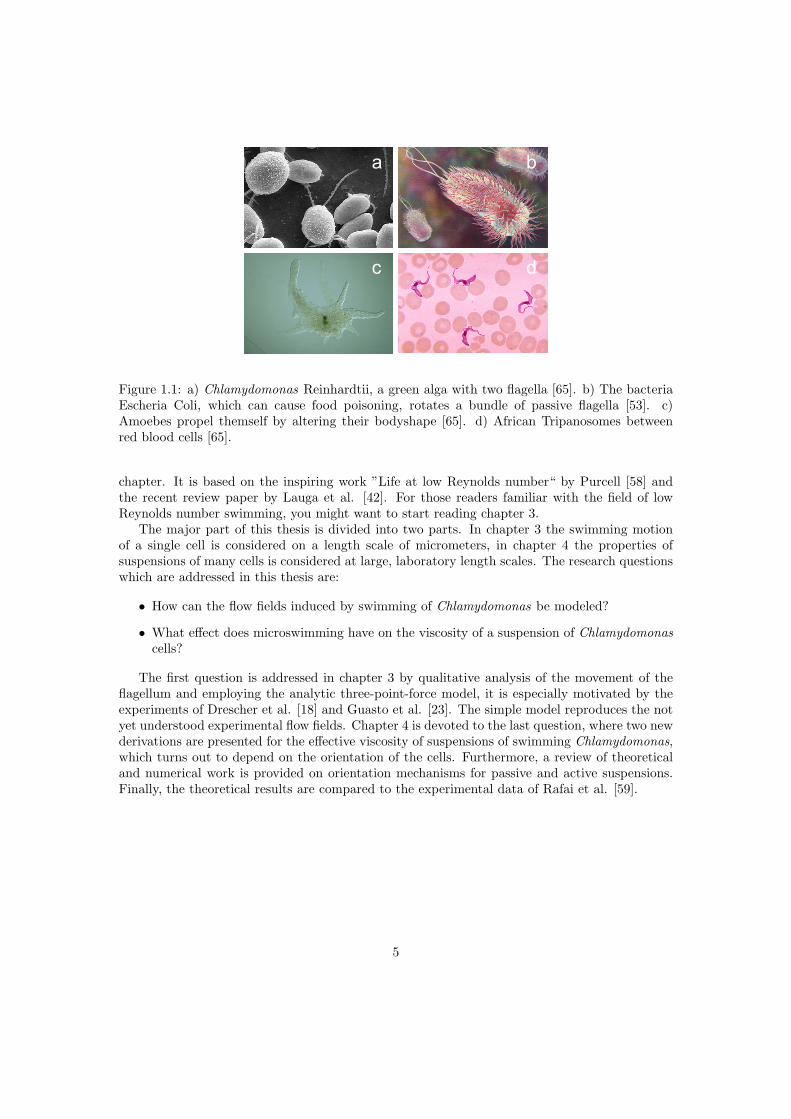
There is an abundancy of life on almost every part of our planet, from penguins on the icy southpole to cactuses in the dry hot deserts and fish in the deepest oceans. This diversity is not limitedto the macroscopic world, visible to our naked eye. When one takes a look with a microscopein the micrometer world, one finds countless fungi, algae, viruses, bacteria, etc. Within ourown body spermatozoa can be regarded as independent acting ’microorganisms’. Many of thesemicroscopic unicellular life forms propel themself in search for a better environment. They mayseek the ovum (egg cell), look for the right light intensity or try to get rid of toxic chemicalsin their neighbourhood. There are several propelling mechanisms, which all have in commonthat they are neither coordinated nor regulated by a brain. Although a lot is known aboutgenetics and cell architecture of microorganisms, the motility of eukaryotes1 is not yet fullyunderstood. All animals, plants, fungi and protists are eukaryotes. We owe our existence tomicroswimming, without a beating flagellum a sperm cell will never reach the ovum. On theother hand microswimmers can cause lethal effects in humans, the African Tripanosome (figure1.1) swimming in the blood stream causes a feared disease known as sleeping sickness.

The extensively studied Chlamydomonas Reinhardti, see figure 1.1, is an eukaryote. Thisgreen unicellular alga has two flagella protruding at the front of its body performing a ’breast-stroke’. Its swimming movement was already recorded in detail 25 years ago [61], but has recentlydrawn attention by experiments conducted on the flow fields induced by swimming on microm-eter length and millisecond time scales [23, 18]. On macroscopic length and timescales viscositymeasurements on suspensions of Chlamydomonas have been performed [59]. There are currentlymany research projects on algae (among which Chlamydomonas ), e.g. as a biofuel producer[48], as a basis for coating [32] and as a basis for feed [31]. Over the last 40 years, theoret-ical research has succesfully treated microswimming in a general way, describing its influenceon macroscopic length scales [63, 26], or by using theoretical swimmers on small length scales[47, 33, 43, 50]. Nonetheless, existing theories do not explain the recent experimental findingson Chlamydomonas on both small and large length scales. The recent experimental observationsand various emerging industrial applications of Chlamydomonas require a more thorough andspecies specific treatment of microswimming.

Microswimming is a fairly new field of physics, which is generally unknown to most physicists.Therefore a general introduction in this topic is provided as background material in the next

1Eukaryotic cells have a membrane and a nucleus.

4

a b

c d

Figure 1.1: a) Chlamydomonas Reinhardtii, a green alga with two flagella [65]. b) The bacteriaEscheria Coli, which can cause food poisoning, rotates a bundle of passive flagella [53]. c)Amoebes propel themself by altering their bodyshape [65]. d) African Tripanosomes betweenred blood cells [65].

chapter. It is based on the inspiring work ”Life at low Reynolds number“ by Purcell [58] andthe recent review paper by Lauga et al. [42]. For those readers familiar with the field of lowReynolds number swimming, you might want to start reading chapter 3.

The major part of this thesis is divided into two parts. In chapter 3 the swimming motionof a single cell is considered on a length scale of micrometers, in chapter 4 the properties ofsuspensions of many cells is considered at large, laboratory length scales. The research questionswhich are addressed in this thesis are:

• How can the flow fields induced by swimming of Chlamydomonas be modeled?

• What effect does microswimming have on the viscosity of a suspension of Chlamydomonascells?

The first question is addressed in chapter 3 by qualitative analysis of the movement of theflagellum and employing the analytic three-point-force model, it is especially motivated by theexperiments of Drescher et al. [18] and Guasto et al. [23]. The simple model reproduces the notyet understood experimental flow fields. Chapter 4 is devoted to the last question, where two newderivations are presented for the effective viscosity of suspensions of swimming Chlamydomonas,which turns out to depend on the orientation of the cells. Furthermore, a review of theoreticaland numerical work is provided on orientation mechanisms for passive and active suspensions.Finally, the theoretical results are compared to the experimental data of Rafai et al. [59].

5

Chapter 2

General physics ofmicroswimming

2.1 Hydrodynamics at low Reynolds number

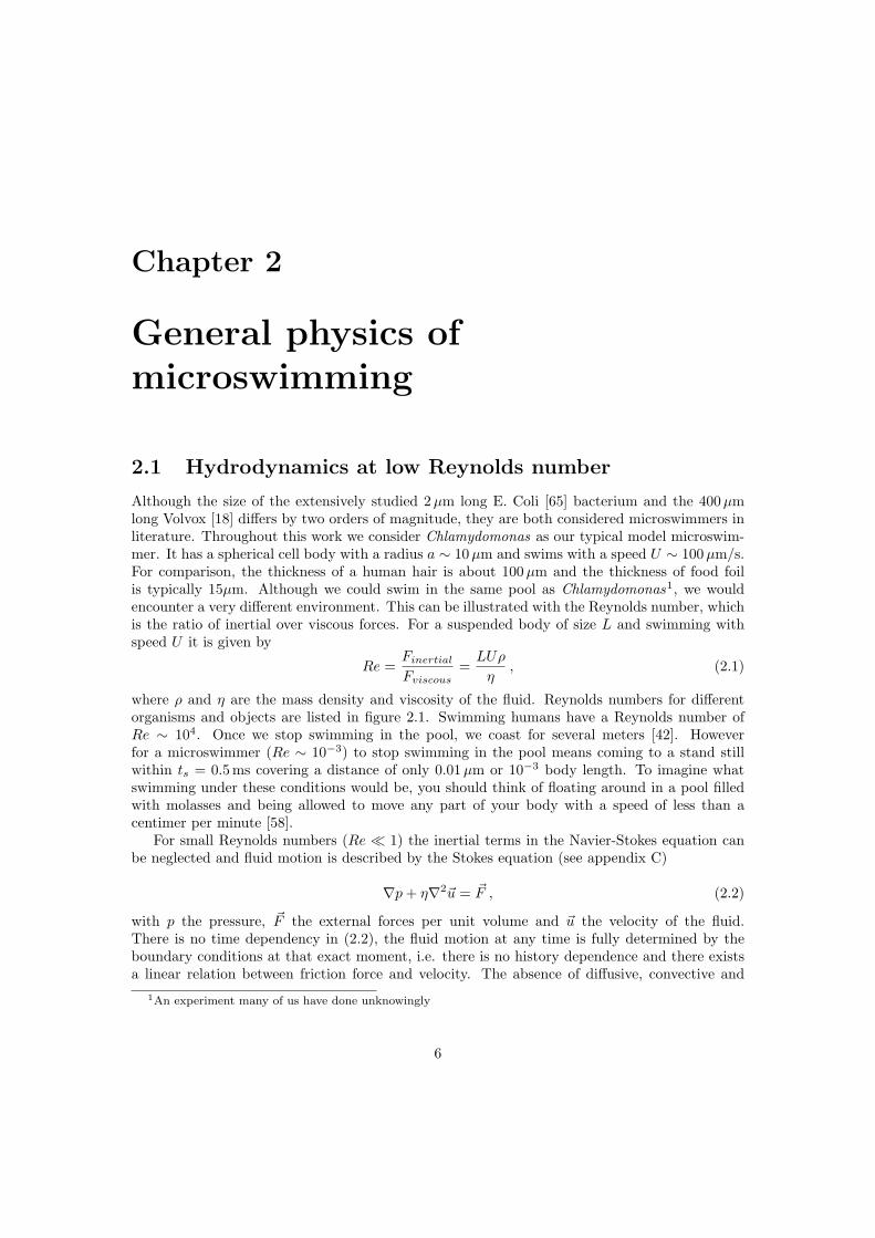
Although the size of the extensively studied 2µm long E. Coli [65] bacterium and the 400µmlong Volvox [18] differs by two orders of magnitude, they are both considered microswimmers inliterature. Throughout this work we consider Chlamydomonas as our typical model microswim-mer. It has a spherical cell body with a radius a ∼ 10µm and swims with a speed U ∼ 100µm/s.For comparison, the thickness of a human hair is about 100µm and the thickness of food foilis typically 15µm. Although we could swim in the same pool as Chlamydomonas1, we wouldencounter a very different environment. This can be illustrated with the Reynolds number, whichis the ratio of inertial over viscous forces. For a suspended body of size L and swimming withspeed U it is given by

Re =FinertialFviscous

=LUρ

η, (2.1)

where ρ and η are the mass density and viscosity of the fluid. Reynolds numbers for differentorganisms and objects are listed in figure 2.1. Swimming humans have a Reynolds number ofRe ∼ 104. Once we stop swimming in the pool, we coast for several meters [42]. Howeverfor a microswimmer (Re ∼ 10−3) to stop swimming in the pool means coming to a stand stillwithin ts = 0.5 ms covering a distance of only 0.01µm or 10−3 body length. To imagine whatswimming under these conditions would be, you should think of floating around in a pool filledwith molasses and being allowed to move any part of your body with a speed of less than acentimer per minute [58].

For small Reynolds numbers (Re 1) the inertial terms in the Navier-Stokes equation canbe neglected and fluid motion is described by the Stokes equation (see appendix C)

∇p+ η∇2~u = ~F , (2.2)

with p the pressure, ~F the external forces per unit volume and ~u the velocity of the fluid.There is no time dependency in (2.2), the fluid motion at any time is fully determined by theboundary conditions at that exact moment, i.e. there is no history dependence and there existsa linear relation between friction force and velocity. The absence of diffusive, convective and

1An experiment many of us have done unknowingly

6

100 m

10 cm

10 μm

2 m

109

102

10-3

104

SizeReynoldsnumber

submarine

sh

human

Chlamydomonas R.

Figure 2.1: The ratio of inertial forces and viscous forces (Reynolds number) for different swim-ming creatures and objects.

time dependent terms in (2.2) allows us to describe the flow as a superposition of elementarysolutions, or Green’s functions, of the Stokes equation.

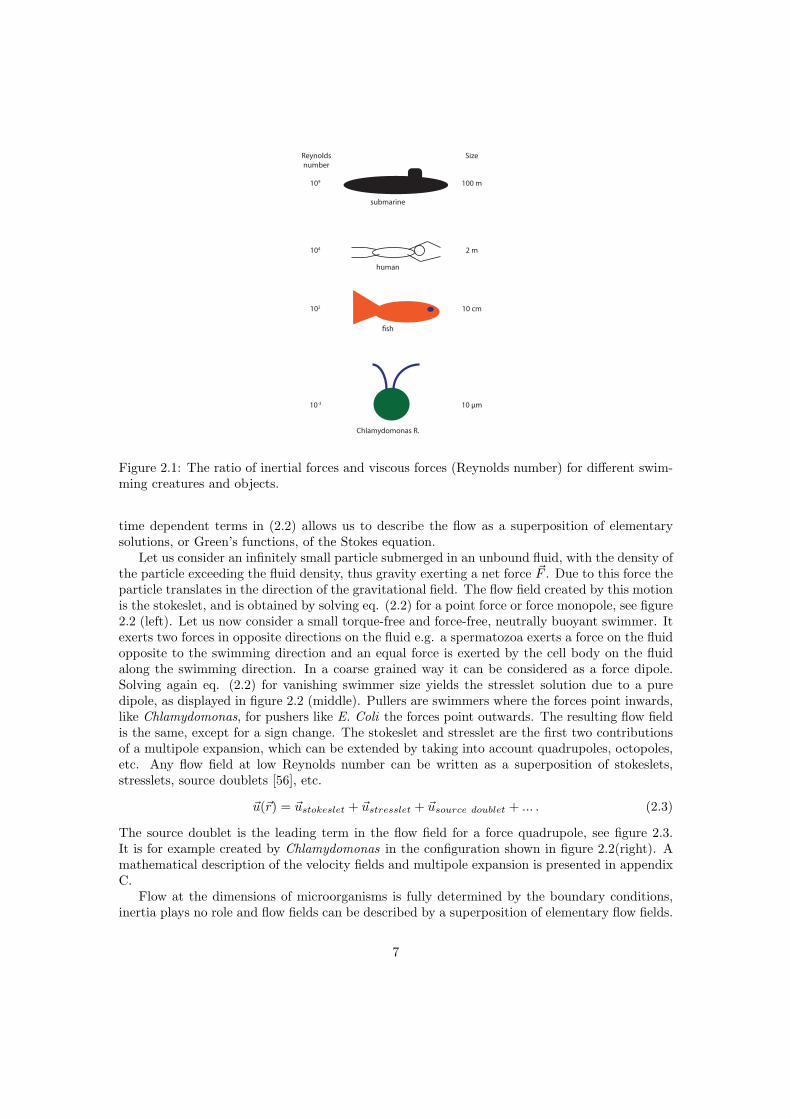
Let us consider an infinitely small particle submerged in an unbound fluid, with the density ofthe particle exceeding the fluid density, thus gravity exerting a net force ~F . Due to this force theparticle translates in the direction of the gravitational field. The flow field created by this motionis the stokeslet, and is obtained by solving eq. (2.2) for a point force or force monopole, see figure2.2 (left). Let us now consider a small torque-free and force-free, neutrally buoyant swimmer. Itexerts two forces in opposite directions on the fluid e.g. a spermatozoa exerts a force on the fluidopposite to the swimming direction and an equal force is exerted by the cell body on the fluidalong the swimming direction. In a coarse grained way it can be considered as a force dipole.Solving again eq. (2.2) for vanishing swimmer size yields the stresslet solution due to a puredipole, as displayed in figure 2.2 (middle). Pullers are swimmers where the forces point inwards,like Chlamydomonas, for pushers like E. Coli the forces point outwards. The resulting flow fieldis the same, except for a sign change. The stokeslet and stresslet are the first two contributionsof a multipole expansion, which can be extended by taking into account quadrupoles, octopoles,etc. Any flow field at low Reynolds number can be written as a superposition of stokeslets,stresslets, source doublets [56], etc.

~u(~r) = ~ustokeslet + ~ustresslet + ~usource doublet + ... . (2.3)

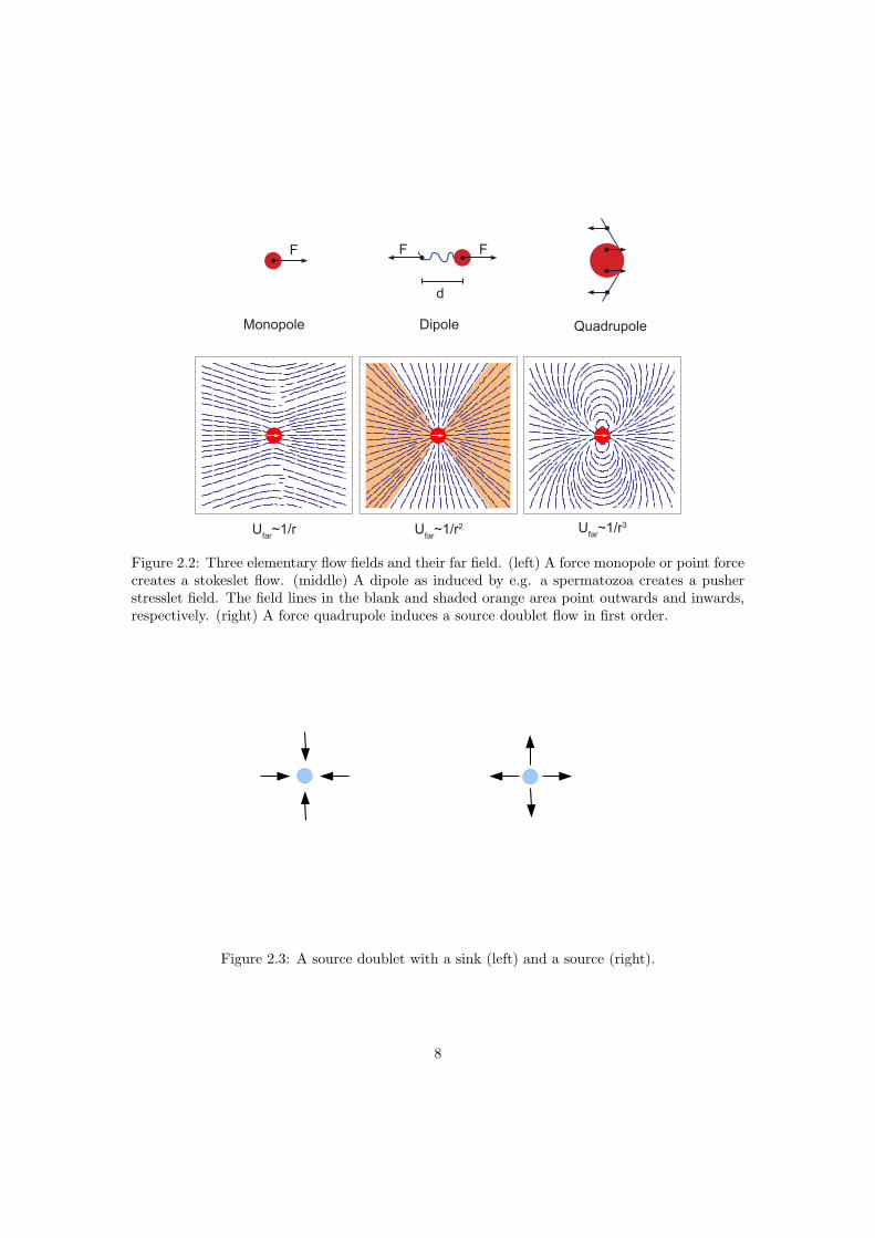
The source doublet is the leading term in the flow field for a force quadrupole, see figure 2.3.It is for example created by Chlamydomonas in the configuration shown in figure 2.2(right). Amathematical description of the velocity fields and multipole expansion is presented in appendixC.

Flow at the dimensions of microorganisms is fully determined by the boundary conditions,inertia plays no role and flow fields can be described by a superposition of elementary flow fields.

7

40 20 0 20 40

40

20

0

20

40

40 20 0 20 40

40

20

0

20

40

40 20 0 20 40

40

20

0

20

40

F F F

d

Monopole Dipole Quadrupole

Ufar~1/r Ufar~1/r2 Ufar~1/r3

Figure 2.2: Three elementary flow fields and their far field. (left) A force monopole or point forcecreates a stokeslet flow. (middle) A dipole as induced by e.g. a spermatozoa creates a pusherstresslet field. The field lines in the blank and shaded orange area point outwards and inwards,respectively. (right) A force quadrupole induces a source doublet flow in first order.

Figure 2.3: A source doublet with a sink (left) and a source (right).

8

gradient

Figure 2.4: A gradient in left-right direction (nutrients, toxic chemicals, etc.) creates a preferredswimming direction. Darker color indicates a more favorable condition for the organism. Whenthe organism swims in the direction of the gradient, it continues swimming in this direction fora longer period of time (red lines).

2.2 Scallop theorem

The time indepencence of the Stokes equation restricts the possible swimming motions. Thiswas elucidated by Purcell [58] with the so-called scallop theorem: a scallop opens its clam slowlyand closes it fast, squirting out water. In the high Reynolds number environment this leads to anet displacement after one opening/closing cycle, but at low Reynolds number it would end upat its exact starting position. This is due to the reciprocal motion of the scallop, a movie of onecycle played backwards looks the same as the movie itself. The time independence of the Stokesequation implies that no matter how fast or slow you move, as long as the Reynolds numberremains small, a reciprocal motion does not result in a net displacement. The micro scallop withone degree of freedom (open/close) is not capable of performing a non-reciprocal motion. Allmicroswimmers perform a non-reciprocal movement, for Chlamydomonas this will be elucidatedin chapter 3.

2.3 Brownian motion, diffusion and random walks

Fluid particles are in constant motion, whereby the average velocity increases with temperature.These fluid particles collide with suspended objects, creating a random movement of the (small)suspended particles, this is called Brownian motion. Brownian motion results in diffusion of thesuspended particle and is described by a diffusion constant for a spherical particle with radius Rgiven by the Stokes-Einstein relation [19]

D =kT

6πηR, (2.4)

with T the temperature and k the Boltzmann constant. The Peclet number is the ratio of timesa particle needs to diffuse a distance L compared to travel the same distance by ballistic motionPe = RU/D. At room temperature (T = 300 K) in water (ηwater = 1 mPa · s ·m) the Peclet

9

number for the typical microswimmer is Pe ' 108, which makes clear that diffusive motion isnegligible for the typical microswimmer. This is no surprise, if you would travel as fast by doingnothing as you would by actively swimming, then why would you swim? The rotary diffusionconstant for a sphere is given by the Stokes-Einstein relation

Dr =kBT

8πηR3. (2.5)

The reciprocal rotary diffusion constant for a typical microswimmer is 1/Dr ∼ 8 · 102 s, whereagain water is used as a suspending medium at room temperature. This indicates that at labtimescales (0.001− 10)s the swimmer (rotary) diffusion is negligible. Many microswimmers usea simple algorithm to ’scan’ their environment. They swim in a straight line for a time ts andafter this time decide to:

• 1. Randomly change direction if conditions have not improved 2

• 2. Remain swimming in the same direction if conditions have improved

This results in a biased random walk [28], see figure 2.4. In this way the organism probes itsvicinity for food, toxic chemicals etc. On longer time scales, i.e. after many reorientation events,a random walk can be described as effective diffusion. For suspensions of Chlamydomonas theeffective diffusion constant was obtained experimentally as Deff = 7 · 10−8 m/s2 and Deff/D ∼106 [55]. The effective rotary diffusion is Dr,eff = 0.4 rad2/s [35] and Dr,eff/Dr ∼ 400.

Microswimmers search for food molecules. The typical size of these biological moleculessoluted in water is ∼ 10 nm. To out-swim diffusion microswimmers have to travel a length scaleldiff = Dbio/U ∼ 100µm [58], where Dbio is the diffusion constant of the biological molecules.This is the typical length after which Chlamydomonas changes its direction.

The diffusion of a microswimmer is negligible compared to the swimming speed. They scantheir environment via a simple random walk algorithm, whereby they outrun diffusion of nutri-ents, chemicals, etc.

2.4 Flagellar propulsion

Amoebes change their body shape and bacteria use a motor to rotate a passive bacterial flagellumto propel themselves [42]. But all eukaryotic microswimmers use one or more active flagella forthe propulsion of their body, see figure 2.5. These flagella have the same basic structure asdisplayed in figure 2.6 which is thought to originate from the mutual eukaryotic ancestor about1-2 billion years ago [52].

The flagellum consists of 2 central microtubuli and 9 outer microtubuli doublets, coveredby a flagellar membrane. The central pair is surrounded by a structure called the central pairapparatus, it is connected with the outer microtubuli doublets via radial spokes which seem toplay a role in altering and regulating the flagellar beat [25]. The dynein motors are connectedto the A microtubulus and reach out to the B microtubulus of the next doublet. Within asingle flagellum over 16 different motors have been reported and the total number of motors in aChlamydomonas flagellum is about 10.000 [25]. The microtubuli are hollow tubes with a diameterof 25 nm, their bending rigidity is about km = 3 · 10−23 Nm2 [1]. In multicellular organisms likehumans, one finds flagella in the spermatozoa, in lungs and throat for dust removal and eventhe left-right asymmetry of our body is caused by the beating of flagella on the surface of the

2The reorientation is not perfectly random: their usually exists a correlation between consecutive swimmingdirections which is species dependent.

10

a b

c d

Figure 2.5: a) Spermatozoa have a flagellum attached to their back (with respect to the swimmingdirection). b) Chlamydomonas has two flagella protruding from the front of its body, c) AfricanTripanosomes have a flagellum which is over the full length of its body attached to the cell.d) An array of cilia which can be found in the respiratory tract of the human body and othermammals.

1

2

3

4

56

7

8

9

Figure 2.6: Schematic overview of a 9+2 flagellum. The central pair microtubuli (inner bluecircles) are surrounded by the central pair apparatus (ellipse). 9 outer microtubuli doublets forma ring, they are numbered 1-9 by convention. The dark and light blue parts are the A and Bmicrotubulus respectively. The dynein motors (red) originate at the A microtubulus and extendtowards the B microtubulus of the next doublet. The radial spokes (orange) originate at the Amicrotubulus too, they are connected with the central pair apparatus.

11

Figure 2.7: Schematic 3D overview of a segment of 96 nm of the axoneme. The flagellum consistsof 1-10000 of these connected segments.

(a) (b)

Figure 2.8: Schematic overview of dynein activity. a) Two microtubuli (blue) are parallel toeach other. When the dynein motors are switched on, the two microtubuli start sliding in thedirection depicted by the two orange arrows. b) The dynein motors have induced sliding, but nobending has occurred.

embryo [25]. Within the body flagella, when they come in arrays and when they are relativelyshort, are called cilia, but their design is the same except for the non-existing central pair, the9+0 flagella/cilia. The length of flagella ranges from 1µm for the smallest cilia to 58000µm [52]in the spermatozoa of fruit flies3. The diameter of the flagellum is constant along the flagellum(200µm). For Chlamydomonas the flagella consist of repeating segments of 96 nm as displayedin figure 2.7.

The dynein motors which are located on all 9 microtubuli doublets are most probably unidi-rectional [25, 12]. The motors on microtubuli i can push microtubuli i− 1 in the direction of thecell body. The dynein activity on itself does not create a bend but merely results in sliding, asillustrated in figure 2.8. Geometrical constraints, created by the attachment to the cell body andthe flagellar structure, are necessary to turn this sliding movement into a bend. This is illustratedin figure 2.9. The organisms considered are unicellular and may have more than 100.000 dyneinunits, but still manage to create complex and sustainable beating patterns. Camalet et al. [14]treated the motors as oscillators and showed that regardless of the microscopic architecture andswitching mechanism a series of oscillators is able to create a sustainable beating pattern. Severalmotor control mechanisms have been proposed [45, 11], succesfully reproducing beating patterns

3it exceeds their bodylength of 1mm

12

(a) (b)

Figure 2.9: a) Two microtubuli (blue) are connected to a wall (green sheet) and additionalgeometrical constraints (green rings) apply. b) The dynein motors (red) are switched on andexert a force, due to the rigid connection to the wall and the geometrical constraints, the motoractivity creates a bend. The length of the microtubuli and the distance between the centerlinesof both tubes is conserved.

for a limited number of organisms. Until now the exact mechanism remains a mystery, as con-cluded by several recent reviews [25, 12, 66, 46]. Many organisms perform a random walk whichis biased by chemicals, nutrients, light intensity etc. This indicates that these organisms havechemical and light sensors which influence the flagellar movement. Eukaryotic microswimmerspropel themselves with flagella, containing many internal motor units. The control mechanismfor the motors is yet unknown.

2.5 Theoretical models

Several theoretical microswimmers have been proposed, which give insight in swimming at lowReynolds number. Investigations range from swim efficiency [44, 8], wall interactions [47], toinfluence of phase difference of cyclic swimmers [2] and swimmer-swimmer interaction of a few[34] or many swimmers [33]. The most important microswimmer models are:

• Taylor sheet An oscillating sheet was shown to move by Taylor [64] as early as 1951.

• Najafi-Golestanian swimmer [50] Three spheres in a row are connected by two linkers,hence it is also known as a two link swimmer. The two links create two degrees of freedom,allowing for non reciprocal movement.

• Squirmer Introduced by Lighthill in 1952 [44] and later developed by Blake [8], it wasused to model spherical swimmers which move by slightly altering their body shape, or forswimming bodies covered by arrays of beating cilia. The induced flow field is a superpositionof the flow induced by a dipole force (stresslet) of strength B2 and the flow induced by aforce quadrupole of strength B1. It is discussed in appendix F.

13

Chapter 3

The motion and induced flows ofChlamydomonas Reinhardtii

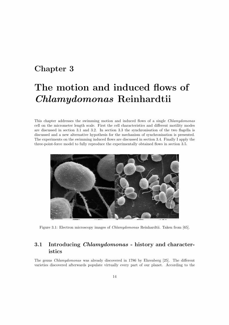
This chapter addresses the swimming motion and induced flows of a single Chlamydomonascell on the micrometer length scale. First the cell characteristics and different motility modesare discussed in section 3.1 and 3.2. In section 3.3 the synchronisation of the two flagella isdiscussed and a new alternative hypothesis for the mechanism of synchronisation is presented.The experiments on the swimming induced flows are discussed in section 3.4. Finally I apply thethree-point-force model to fully reproduce the experimentally obtained flows in section 3.5.

Figure 3.1: Electron microscopy images of Chlamydomonas Reinhardtii. Taken from [65].

3.1 Introducing Chlamydomonas - history and character-istics

The genus Chlamydomonas was already discovered in 1786 by Ehrenberg [25]. The differentvarieties discovered afterwards populate virtually every part of our planet. According to the

14

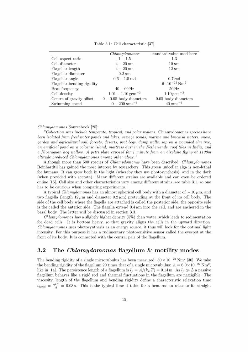
Table 3.1: Cell characteristic [37]

Chlamydomonas standard value used hereCell aspect ratio 1− 1.5 1.3Cell diameter 4− 20µm 10µmFlagellar length 4− 20µm 12µmFlagellar diameter 0.2µmFlagellar angle 0.6− 1.5 rad 0.7 radFlagellar bending rigidity 6 · 10−22 Nm2

Beat frequency 40− 60 Hz 50 HzCell density 1.01− 1.10 gcm−3 1.10 gcm−3

Centre of gravity offset 0− 0.05 body diameters 0.05 body diametersSwimming speed 0− 200µms−1 40µms−1

Chlamydomonas Sourcebook [25]:”Collection sites include temperate, tropical, and polar regions. Chlamydomonas species have

been isolated from freshwater ponds and lakes, sewage ponds, marine and brackish waters, snow,garden and agricultural soil, forests, deserts, peat bogs, damp walls, sap on a wounded elm tree,an artificial pond on a volcanic island, mattress dust in the Netherlands, roof tiles in India, anda Nicaraguan hog wallow. A petri plate exposed for 1 minute from an airplane flying at 1100maltitude produced Chlamydomonas among other algae.“

Although more than 500 species of Chlamydomonas have been described, ChlamydomonasReinhardtii has gained the most interest by researchers. This green unicellar alga is non-lethalfor humans. It can grow both in the light (whereby they use photosynthesis), and in the dark(when provided with acetate). Many different strains are available and can even be orderedonline [15]. Cell size and other characteristics vary among different strains, see table 3.1, so onehas to be cautious when comparing experiments.

A typical Chlamydomonas has an almost spherical cell body with a diameter of ∼ 10µm, andtwo flagella (length 12µm and diameter 0.2µm) protruding at the front of its cell body. Theside of the cell body where the flagella are attached is called the posterior side, the opposite sideis the called the anterior side. The flagella extend 0.4µm into the cell, and are anchored in thebasal body. The latter will be discussed in section 3.3.

Chlamydomonas has a slightly higher density (5%) than water, which leads to sedimentationfor dead cells. It is bottom heavy, so that gravity aligns the cells in the upward direction.Chlamydomonas uses photosynthesis as an energy source, it thus will look for the optimal lightintensity. For this purpose it has a rudimentary photosensitive sensor called the eyespot at thefront of its body. It is connected with the central pair of the flagellum.

3.2 The Chlamydomonas flagellum & motility modes

The bending rigidity of a single microtubulus has been measured: 30× 10−24 Nm2 [30]. We takethe bending rigidity of the flagellum 20 times that of a single microtubulus: A = 6.0×10−22 Nm2,like in [14]. The persistence length of a flagellum is lp = A/(kBT ) = 0.14 m. As lp L a passiveflagellum behaves like a rigid rod and thermal fluctuations in the flagellum are negligible. Theviscosity, length of the flagellum and bending rigidity define a characteristic relaxation timetbend = ηL4

A = 0.03 s. This is the typical time it takes for a bent rod to relax to its straight

15

equilibrium configuration in a viscous environment. Note that it is longer than the beat cycletime tbeat ∼ 0.02 s, during the beating cycle the flagellum is not able to relax to an equilibriumstate. Chlamydomonas displays several motility modes:

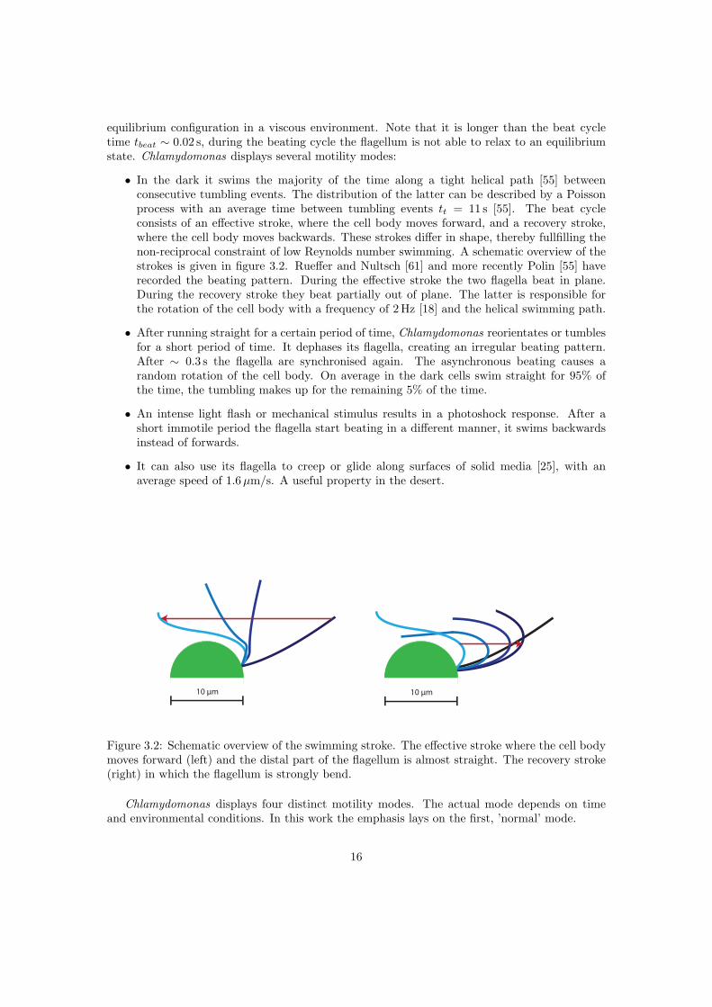
• In the dark it swims the majority of the time along a tight helical path [55] betweenconsecutive tumbling events. The distribution of the latter can be described by a Poissonprocess with an average time between tumbling events tt = 11 s [55]. The beat cycleconsists of an effective stroke, where the cell body moves forward, and a recovery stroke,where the cell body moves backwards. These strokes differ in shape, thereby fullfilling thenon-reciprocal constraint of low Reynolds number swimming. A schematic overview of thestrokes is given in figure 3.2. Rueffer and Nultsch [61] and more recently Polin [55] haverecorded the beating pattern. During the effective stroke the two flagella beat in plane.During the recovery stroke they beat partially out of plane. The latter is responsible forthe rotation of the cell body with a frequency of 2 Hz [18] and the helical swimming path.

• After running straight for a certain period of time, Chlamydomonas reorientates or tumblesfor a short period of time. It dephases its flagella, creating an irregular beating pattern.After ∼ 0.3 s the flagella are synchronised again. The asynchronous beating causes arandom rotation of the cell body. On average in the dark cells swim straight for 95% ofthe time, the tumbling makes up for the remaining 5% of the time.

• An intense light flash or mechanical stimulus results in a photoshock response. After ashort immotile period the flagella start beating in a different manner, it swims backwardsinstead of forwards.

• It can also use its flagella to creep or glide along surfaces of solid media [25], with anaverage speed of 1.6µm/s. A useful property in the desert.

10 μm 10 μm

Figure 3.2: Schematic overview of the swimming stroke. The effective stroke where the cell bodymoves forward (left) and the distal part of the flagellum is almost straight. The recovery stroke(right) in which the flagellum is strongly bend.

Chlamydomonas displays four distinct motility modes. The actual mode depends on timeand environmental conditions. In this work the emphasis lays on the first, ’normal’ mode.

16

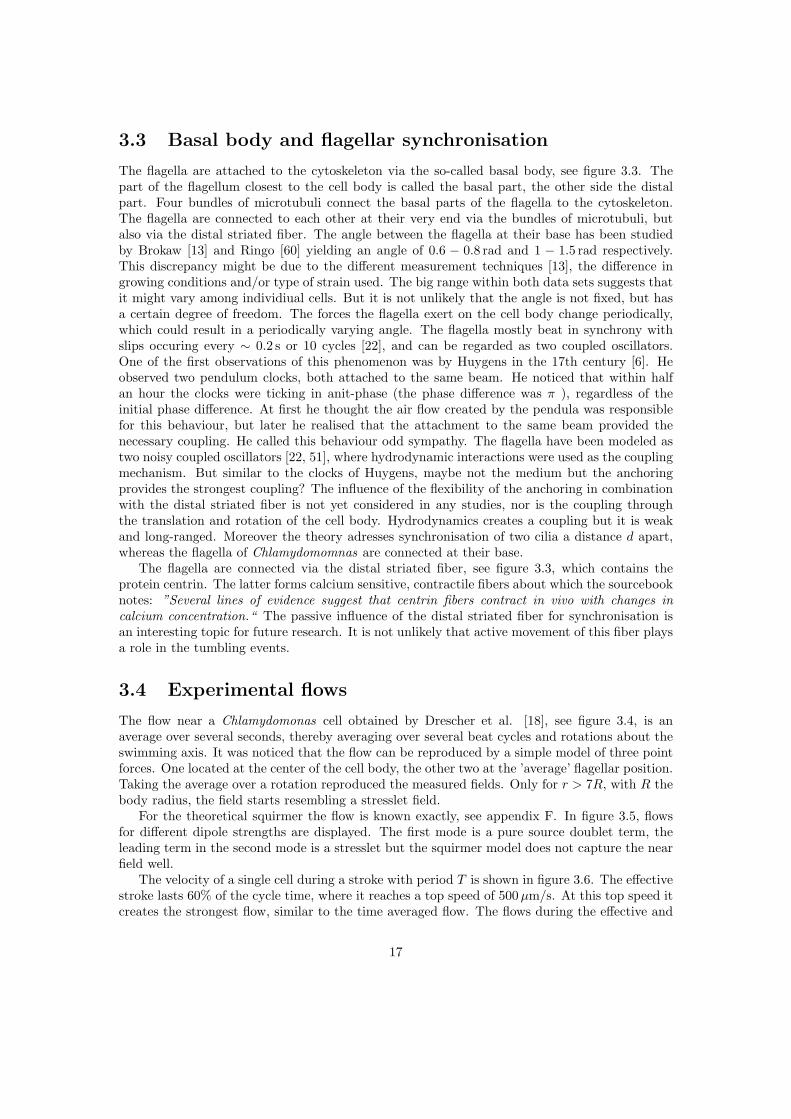
3.3 Basal body and flagellar synchronisation

The flagella are attached to the cytoskeleton via the so-called basal body, see figure 3.3. Thepart of the flagellum closest to the cell body is called the basal part, the other side the distalpart. Four bundles of microtubuli connect the basal parts of the flagella to the cytoskeleton.The flagella are connected to each other at their very end via the bundles of microtubuli, butalso via the distal striated fiber. The angle between the flagella at their base has been studiedby Brokaw [13] and Ringo [60] yielding an angle of 0.6 − 0.8 rad and 1 − 1.5 rad respectively.This discrepancy might be due to the different measurement techniques [13], the difference ingrowing conditions and/or type of strain used. The big range within both data sets suggests thatit might vary among individiual cells. But it is not unlikely that the angle is not fixed, but hasa certain degree of freedom. The forces the flagella exert on the cell body change periodically,which could result in a periodically varying angle. The flagella mostly beat in synchrony withslips occuring every ∼ 0.2 s or 10 cycles [22], and can be regarded as two coupled oscillators.One of the first observations of this phenomenon was by Huygens in the 17th century [6]. Heobserved two pendulum clocks, both attached to the same beam. He noticed that within halfan hour the clocks were ticking in anit-phase (the phase difference was π ), regardless of theinitial phase difference. At first he thought the air flow created by the pendula was responsiblefor this behaviour, but later he realised that the attachment to the same beam provided thenecessary coupling. He called this behaviour odd sympathy. The flagella have been modeled astwo noisy coupled oscillators [22, 51], where hydrodynamic interactions were used as the couplingmechanism. But similar to the clocks of Huygens, maybe not the medium but the anchoringprovides the strongest coupling? The influence of the flexibility of the anchoring in combinationwith the distal striated fiber is not yet considered in any studies, nor is the coupling throughthe translation and rotation of the cell body. Hydrodynamics creates a coupling but it is weakand long-ranged. Moreover the theory adresses synchronisation of two cilia a distance d apart,whereas the flagella of Chlamydomomnas are connected at their base.

The flagella are connected via the distal striated fiber, see figure 3.3, which contains theprotein centrin. The latter forms calcium sensitive, contractile fibers about which the sourcebooknotes: ”Several lines of evidence suggest that centrin fibers contract in vivo with changes incalcium concentration.“ The passive influence of the distal striated fiber for synchronisation isan interesting topic for future research. It is not unlikely that active movement of this fiber playsa role in the tumbling events.

3.4 Experimental flows

The flow near a Chlamydomonas cell obtained by Drescher et al. [18], see figure 3.4, is anaverage over several seconds, thereby averaging over several beat cycles and rotations about theswimming axis. It was noticed that the flow can be reproduced by a simple model of three pointforces. One located at the center of the cell body, the other two at the ’average’ flagellar position.Taking the average over a rotation reproduced the measured fields. Only for r > 7R, with R thebody radius, the field starts resembling a stresslet field.

For the theoretical squirmer the flow is known exactly, see appendix F. In figure 3.5, flowsfor different dipole strengths are displayed. The first mode is a pure source doublet term, theleading term in the second mode is a stresslet but the squirmer model does not capture the nearfield well.

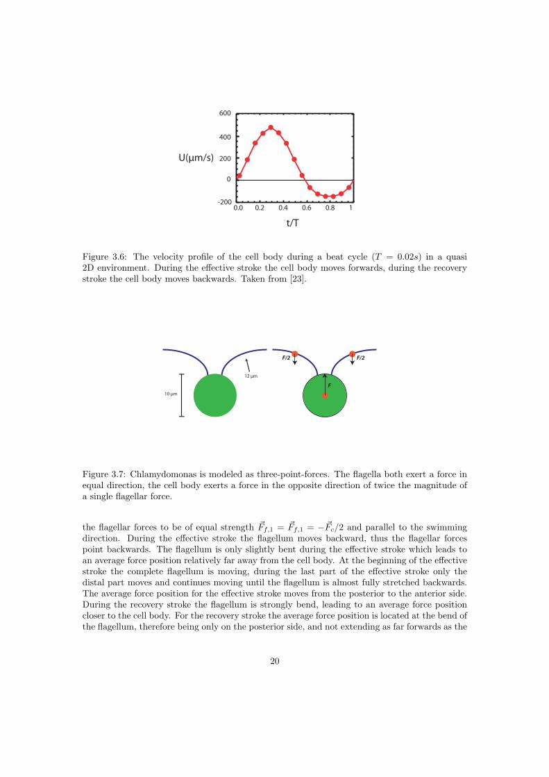
The velocity of a single cell during a stroke with period T is shown in figure 3.6. The effectivestroke lasts 60% of the cycle time, where it reaches a top speed of 500µm/s. At this top speed itcreates the strongest flow, similar to the time averaged flow. The flows during the effective and

17

Figure 3.3: The basal parts (bb) of the flagella are attached to the cytoskeleton via four bundlesof microtubuli (MTR). The distal striated fiber (DSF) creates a second intra flagellar connection.Taken from [25].

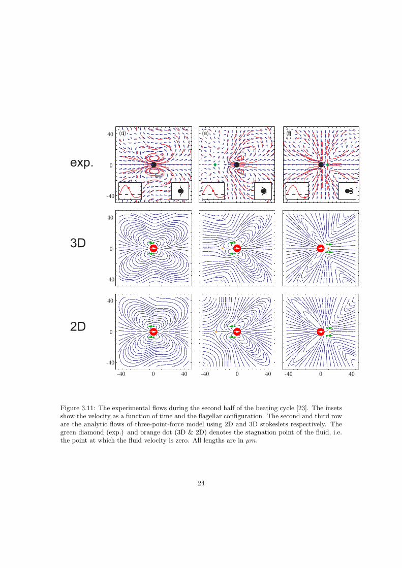
recovery stroke show a strong time-dependence and have been obtained by Guasto et al. [23],see figure 3.10 and 3.11. This highly time-dependent flow field was not yet understood, in thenext section I present a simple model which reproduces the flow fields in full detail.

3.5 Three-point-force model

During the beating cycle both the flagella exert a force on the fluid, and the cell body also exertsa force on the fluid. The three-point-force model reduces a Chlamydomonas cell to these threeforces, see figure 3.7. The magnitude of the force a flagellum exerts is calculated by integratingthe force density ~f per unit length of the flagellum:

~Fi =∫S

~fidsi , i = 1, 2 , (3.1)

where s is the distance of a point on the flagellum measured along the flagellum, see figure 3.8.As the cell is force-free (

∑ ~Fi = 0), the cell body exerts a force ~Fc = −(~Ff,1 + ~Ff,2) on the fluid.Regarding Chlamydomonas as a sphere, the force ~Fc = 6πηRUp on the cell body is calculatedusing the velocity of the cell, see figure 3.6, with p the unit vector along the swimming direction.The cell body force is exerted at the center of the cell body, the positions where the flagellarforces are exerted change during the beating cycle. I introduce the flagellar force positions as:

sf,i =

∫Ssi ~fdsi∫S~fdsi

, (3.2)

whereby the curve S changes during the beating cycle. The force densities can be estimatedusing video analysis of the stroke, as has been done for spermatozoa [21]. However, I assume

18

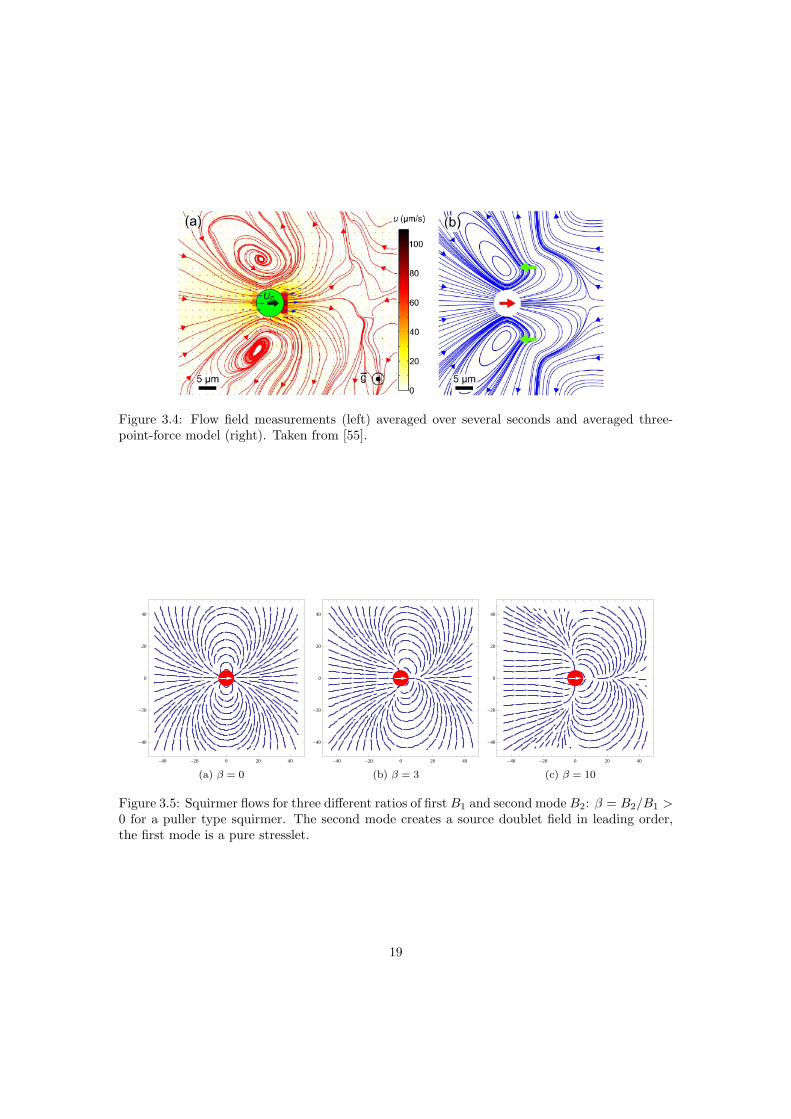
Figure 3.4: Flow field measurements (left) averaged over several seconds and averaged three-point-force model (right). Taken from [55].

-40 -20 0 20 40

-40

-20

0

20

40

(a) β = 0

-40 -20 0 20 40

-40

-20

0

20

40

(b) β = 3

-40 -20 0 20 40

-40

-20

0

20

40

(c) β = 10

Figure 3.5: Squirmer flows for three different ratios of first B1 and second mode B2: β = B2/B1 >0 for a puller type squirmer. The second mode creates a source doublet field in leading order,the first mode is a pure stresslet.

19

t/T

0.2 0.4 0.6 0.80.0 1-200

0

200

400

600

U(μm/s)

Figure 3.6: The velocity profile of the cell body during a beat cycle (T = 0.02s) in a quasi2D environment. During the effective stroke the cell body moves forwards, during the recoverystroke the cell body moves backwards. Taken from [23].

10 μm

12 μm

F

F/2 F/2

Figure 3.7: Chlamydomonas is modeled as three-point-forces. The flagella both exert a force inequal direction, the cell body exerts a force in the opposite direction of twice the magnitude ofa single flagellar force.

the flagellar forces to be of equal strength ~Ff,1 = ~Ff,1 = −~Fc/2 and parallel to the swimmingdirection. During the effective stroke the flagellum moves backward, thus the flagellar forcespoint backwards. The flagellum is only slightly bent during the effective stroke which leads toan average force position relatively far away from the cell body. At the beginning of the effectivestroke the complete flagellum is moving, during the last part of the effective stroke only thedistal part moves and continues moving until the flagellum is almost fully stretched backwards.The average force position for the effective stroke moves from the posterior to the anterior side.During the recovery stroke the flagellum is strongly bend, leading to an average force positioncloser to the cell body. For the recovery stroke the average force position is located at the bend ofthe flagellum, therefore being only on the posterior side, and not extending as far forwards as the

20

S

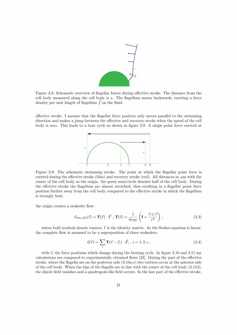
Figure 3.8: Schematic overview of flagellar forces during effective stroke. The distance from thecell body measured along the cell body is s. The flagellum moves backwards, exerting a forcedensity per unit length of flagellum ~f on the fluid.

effective stroke. I assume that the flagellar force position only moves parallel to the swimmingdirection and makes a jump between the effective and recovery stroke when the speed of the cellbody is zero. This leads to a beat cycle as shown in figure 3.9. A single point force exerted at

-5

7

5

0 3 5 9 10

Figure 3.9: The schematic swimming stroke. The point at which the flagellar point force isexerted during the effective stroke (blue) and recovery stroke (red). All distances in µm with thecenter of the cell body as the origin. the green semi-circle denotes half of the cell body. Duringthe effective stroke the flagellum are almost stretched, thus resulting in a flagellar point forceposition further away from the cell body compared to the effective stroke in which the flagellumis strongly bent.

the origin creates a stokeslet flow:

~uSto,3D(~r) = T(~r) · ~F , T(~r) =1

8πηr

(I +

~r ⊗ ~rr2

), (3.3)

where bold symbols denote tensors, I is the identity matrix. As the Stokes equation is linear,the complete flow is assumed to be a superposition of three stokeslets:

~u(~r) =∑i

T(~r − ~ri) · ~Fi , i = 1, 2, c , (3.4)

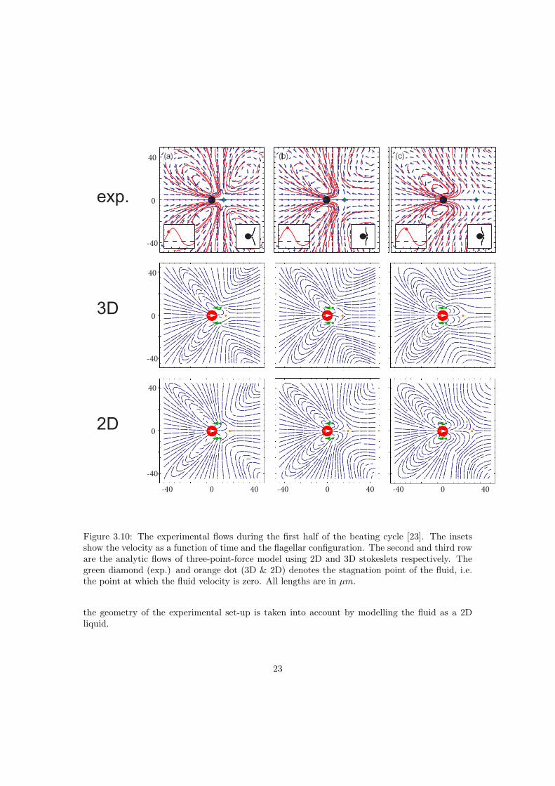
with ~ri the force positions which change during the beating cycle. In figure 3.10 and 3.11 mycalculations are compared to experimentally obtained flows [23]. During the part of the effectivestroke, where the flagella are on the posterior side (3.10a-c) two vortices occur at the anterior sideof the cell body. When the tips of the flagella are in line with the center of the cell body (3.11d),the dipole field vanishes and a quadrupole-like field occurs. In the last part of the effective stroke,

21

where the flagella are at the anterior side (3.11e), the two vertices occur on the posterior side ofthe cell body. For the recovery stroke (3.11f) the field is similar to that of the first part of theeffective stroke except for a sign change. The simple 3D model shows good agreement with theexperiments. The experiments of Guasto et al. [23] were performed in a thin liquid film boundedby two liquid-air interfaces. The diameter of the cell body of the Chlamydomonas used in thisexperiment was 7−10µm and the width of the film 15±2µm. Only cells where the flagella werebeating in a plane parallel to the interfaces were tracked. For soap films with suspended particlesa transition occurs between three dimensional and two dimensional behaviour. By comparingthe diffusion of particles of size d in a film with a thickness h the self diffusion showed a 2D-3Dtransition at a ratio h/d = 7 ± 3 [57]. For the Chlamydomonas experiments h/d = 2, clearlybelow this empirical limit. In the Chlamydomonas thin film experiments it was noted that thefar field scaled like u ∼ 1/r which is a clear 2D effect, a dipole field in 3D decays like u ∼ 1/r2,see appendix C. A two dimensional stokeslet due to a point force exists [56]

~uSto2D(~r) = T(~r) · ~F , T(~r) =1

4πη

(−ln

(r

r0

)I +

~r ⊗ ~rr2

), (3.5)

where r0 is a length scale, it is an undetermined constant as there is no typical length scale in aninfinite 2D liquid. For a superposition of point forces like in the 3D model the flow is independentof r0 as long as

∑i~Fi = 0, see appendix C.

Substituting the 2D Stokeslet in the three-point-force model creates even better agreementwith experiments, see figure 3.10 and 3.11. Although the 2D Stokeslet can be deduced mathe-matically, the physical interpretation is not clear. The 2D problem of a point force is equivalentto an infinitely line in 3D where a constant force density per unit of length is exerted. A solutionof the Stokes equation for this problem does not exist, the infinite long line force results in aninfinite Reynolds number, regardless of the magnitude of the force density. This is known asthe Stokes paradox. Nonetheless using a 3D Stokeslet for a thin film is a gross approximationtoo, and the 2D stokeslet model shows better agreement. A solution would be to use the 3Dstokeslet and incorporate the reflections at the interfaces. Analytic solutions for the flow inducedby a point force between two rigid walls exist, but is complex [38]. Simpler approximations existfor a point force near a single wall [7], but they only predict the flow well for relatively largeseparations, which is not the case for the experimental set-up. Besides, the fluid-air interfaceis not actually a rigid wall, as only the normal component of the fluid velocity is zero at theinterface, which is a strong motivation to describe the system as a 2D fluid.

The time-averaged flow field in figure 3.4 can be obtained by a weighted average of the timedependent three-point-force model, thereby also averaging about a rotation about its swimmingdirection. The weighting factor is the magnitude of the force obtained from the swimming speed,see figure 3.6.

The simple three point model does not incorporate interactions between the flagella, cell bodynor with externally applied flows. A more detailed description of average positions during thebeat cycle and taking into account the transverse forces exerted by the flagella might improvethe results, but the simple model presented here explains the experiments within experimentalerrors. Also the flow around the cell body due to the no-slip boundaries is already more complexthan a simple Stokeslet, there is a source doublet contribution. But zooming in this much theasphericity and visco elasticity of the cell body might affect the flow field too.In this chapter I have presented a new hypothesis for the synchronisation of the flagella, it mightnot be due to the hydrodynamic interactions between the flagella but due to the connection ofthe flagella both at their base and via the distal striated fiber. Using a schematic analysis of theswimming stroke of Chlamydomonas I have presented a simple three-point-force model whichreproduces the full details of the highly time dependent swimming induced flow fields, whereby

22

speed decreases rapidly near the hyperbolic stagnationpoint 7–8 radii from the swimmer.

The time-averaged velocity field in Fig. 2(a) shows thelimitations of some current swimmer models, as also notedin [6], and raises several important questions. For example,how does the velocity field evolve throughout the oscilla-tory flagellar beat cycle? Using high-speed imaging(500 fps), we measure the instantaneous swimmer phase,and identify tracer particles at corresponding times in thebeat cycle. Velocity fields (resulting from 170 cell tracks)are constructed from tracer velocities at each phase of theoscillation with resolution T=15.

A time series of the velocity field during the beat cycle isshown in Fig. 3 (see video [15]). Insets show swimmerspeed and phase (lower left) and approximate flagellarposition (lower right). At the beginning of the power stroke[Fig. 3(a)], the velocity field is neatly divided into foursymmetric quadrants with the hyperbolic stagnation pointlocated slightly forward from the body, in line with con-ventional force dipole swimmer models [1]. As the flagellamove toward the posterior and the power stroke peaks, thevortices lateral to the organism strengthen [Fig. 3(b)], then

shift across the body to the anterior side [Fig. 3(c)–3(e)].After the power stroke ends and the recovery stroke begins,the flagella extend out in front of the organism, and the cellvelocity becomes negative. The flow shown in Fig. 3(f) isqualitatively reversed from Fig. 3(a), changing the sign ofthe dipole. The instantaneous flow field generated by anoscillatory swimmer such as C. reinhardtii is complex andhighly time dependent.In Stokes flows, all of the mechanical energy generated

by a swimmer for locomotion is rapidly dissipated by thefluid. The power transferred to the fluid by the organism iscalculated from the velocity field gradient through theviscous dissipation P ¼ R

2ð:ÞhdA, where is the

fluid viscosity, ¼ 12 ½ruþ ðruÞT is the rate of strain

tensor, and dA is a differential area element of the film[15]. The instantaneous mechanical power output, PoscðtÞ,is calculated from the velocity fields [Fig. 3] throughout thebeat cycle and shown in Fig. 4(a). The peak power output(15 fW) occurs during the power stroke and correspondsto the maximum instantaneous speed of the cell body. Asecondary local maximum also occurs at the peak speed ofthe recovery stroke [see Fig. 4(b) (inset)]. Because of the

FIG. 3 (color online). Time sequence of the velocity field evolution throughout the beat cycle (period T ¼ 18:9 ms) of C. reinhardtii(oriented to the right) including the hyperbolic stagnation point position (green diamond). Insets show cell speed and beat cycle phase[lower left, see Fig. 4(b) for details], and approximate flagellar shape (lower right, measured separately). (a) Early in the power stroke,the velocity field resembles a (negative) force dipole. (b) At the peak of the power stroke, the vortices lateral to the organism strengthenand sweep toward the posterior. (c)–(e) The vortices then shift to the anterior as the power stroke is completed. (f) At the peak of therecovery stroke, the flow field again takes the shape of a dipole, but with opposite sign. The recovery stroke velocity field (f) is weakerthan the forward stroke, but is enhanced by the log scaling [20].

PRL 105, 168102 (2010) P HY S I CA L R EV I EW LE T T E R Sweek ending

15 OCTOBER 2010

168102-3











15 OCTOBER 2010

168102-3











15 OCTOBER 2010

168102-3

exp.

3D

2D

0 40-40 0 40-40 0 40-40

0

-40

40

0

-40

40

0

-40

40

Figure 3.10: The experimental flows during the first half of the beating cycle [23]. The insetsshow the velocity as a function of time and the flagellar configuration. The second and third roware the analytic flows of three-point-force model using 2D and 3D stokeslets respectively. Thegreen diamond (exp.) and orange dot (3D & 2D) denotes the stagnation point of the fluid, i.e.the point at which the fluid velocity is zero. All lengths are in µm.

the geometry of the experimental set-up is taken into account by modelling the fluid as a 2Dliquid.

23











15 OCTOBER 2010

168102-3











15 OCTOBER 2010

168102-3











15 OCTOBER 2010

168102-3

exp.

3D

2D

0 40-40 0 40-40 0 40-40

0

-40

40

0

-40

40

0

-40

40

Figure 3.11: The experimental flows during the second half of the beating cycle [23]. The insetsshow the velocity as a function of time and the flagellar configuration. The second and third roware the analytic flows of three-point-force model using 2D and 3D stokeslets respectively. Thegreen diamond (exp.) and orange dot (3D & 2D) denotes the stagnation point of the fluid, i.e.the point at which the fluid velocity is zero. All lengths are in µm.

24

Chapter 4

Rheology of a suspension ofChlamydomonas Reinhardtii

The previous chapter addressed the swimming motion and induced flows on the micrometerscale, this chapter focuses on the macroscopic influence of swimming of Chlamydomonas. Aftera short introduction of viscosity and the cone-plate rheometer in sections 4.1 & 4.2, I continuewith presenting an overview of theory on the effective viscosity of dilute passive suspensionsin section 4.3 treating both gravitational and shape effects. In section 4.4 two new derivationsare provided for the effect of swimming on the viscosity of dilute suspensions by application ofthe three-point-force model. The viscosity will turn out to depend on the average swimmingdirection. A literature study on the latter is presented incorporating both shape and gravityas well as rotary diffusion. A comparison is made between theory and experiments in section4.6, and numerical results are discussed in 4.7. Finally in section 4.8 non-dilute suspensions arebriefly addressed. My contribution consists of two new derivations for the effective viscosity of asuspension of Chlamydomonas cells and a review of existing literature on this topic.

4.1 What is viscosity?

The viscosity of a fluid describes the resistance of a fluid to applied shear stresses. Let us considerthe experiment of section 2.1 of swimming in molasses. It will be much harder to move yourlimbs in molasses than in a regular swimming pool filled with water, due to the higher viscosity ofmolasses. The viscosity is a measure of the microscopic interactions and the momentum transferat the molecular level. Macroscopically, it relates the strain rate to the stress tensor. For aNewtonian fluid the latter is

σ = −pI + 2ηe , (4.1)

with p the pressure, η the viscosity and the strain rate tensor is given by

e =12

(∇~u+ (∇~u)T ) . (4.2)

The area of physics considering the behaviour of complex fluids under shear deformations iscalled “rheology”.

25

4.2 Cone-plate rheometer and simple shear flow

cone

plate

fluid

ω

θr

z

Figure 4.1: A schematic overview of a cone-plate rheometer.

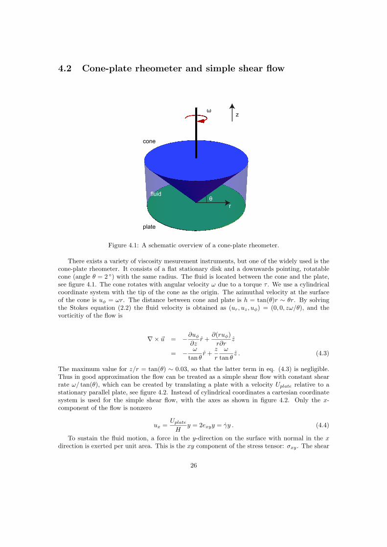
There exists a variety of viscosity mesurement instruments, but one of the widely used is thecone-plate rheometer. It consists of a flat stationary disk and a downwards pointing, rotatablecone (angle θ = 2 ) with the same radius. The fluid is located between the cone and the plate,see figure 4.1. The cone rotates with angular velocity ω due to a torque τ . We use a cylindricalcoordinate system with the tip of the cone as the origin. The azimuthal velocity at the surfaceof the cone is uφ = ωr. The distance between cone and plate is h = tan(θ)r ∼ θr. By solvingthe Stokes equation (2.2) the fluid velocity is obtained as (ur, uz, uφ) = (0, 0, zω/θ), and thevorticitiy of the flow is

∇× ~u = −∂uφ∂z

r +∂(ruφ)r∂r

z

= − ω

tan θr +

z

r

ω

tan θz . (4.3)

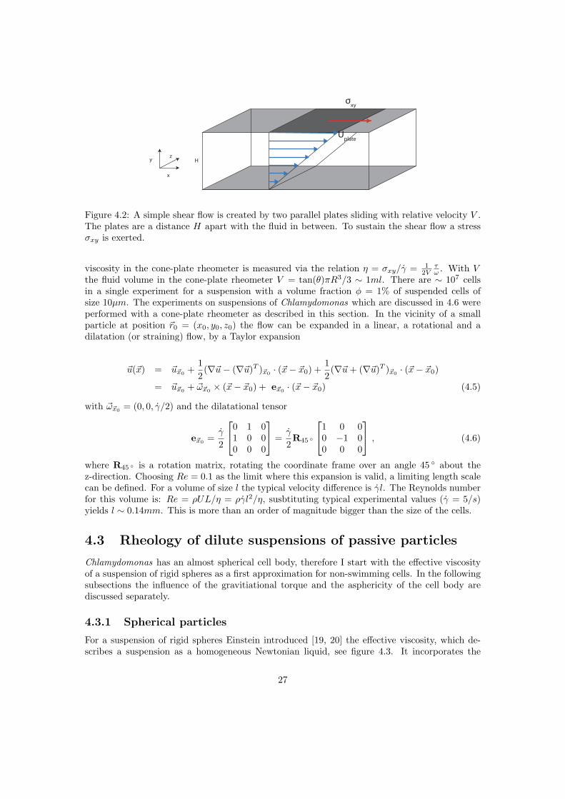
The maximum value for z/r = tan(θ) ∼ 0.03, so that the latter term in eq. (4.3) is negligible.Thus in good approximation the flow can be treated as a simple shear flow with constant shearrate ω/ tan(θ), which can be created by translating a plate with a velocity Uplate relative to astationary parallel plate, see figure 4.2. Instead of cylindrical coordinates a cartesian coordinatesystem is used for the simple shear flow, with the axes as shown in figure 4.2. Only the x-component of the flow is nonzero

ux =UplateH

y = 2exyy = γy . (4.4)

To sustain the fluid motion, a force in the y-direction on the surface with normal in the xdirection is exerted per unit area. This is the xy component of the stress tensor: σxy. The shear

26

σxy

x

y zH

Uplate

Figure 4.2: A simple shear flow is created by two parallel plates sliding with relative velocity V .The plates are a distance H apart with the fluid in between. To sustain the shear flow a stressσxy is exerted.

viscosity in the cone-plate rheometer is measured via the relation η = σxy/γ = 12V

τω . With V

the fluid volume in the cone-plate rheometer V = tan(θ)πR3/3 ∼ 1ml. There are ∼ 107 cellsin a single experiment for a suspension with a volume fraction φ = 1% of suspended cells ofsize 10µm. The experiments on suspensions of Chlamydomonas which are discussed in 4.6 wereperformed with a cone-plate rheometer as described in this section. In the vicinity of a smallparticle at position ~r0 = (x0, y0, z0) the flow can be expanded in a linear, a rotational and adilatation (or straining) flow, by a Taylor expansion

~u(~x) = ~u~x0 +12

(∇~u− (∇~u)T )~x0 · (~x− ~x0) +12

(∇~u+ (∇~u)T )~x0 · (~x− ~x0)

= ~u~x0 + ~ω~x0 × (~x− ~x0) + e~x0 · (~x− ~x0) (4.5)

with ~ω~x0 = (0, 0, γ/2) and the dilatational tensor

e~x0 =γ

2

0 1 01 0 00 0 0

=γ

2R45

1 0 00 −1 00 0 0

, (4.6)

where R45 is a rotation matrix, rotating the coordinate frame over an angle 45 about thez-direction. Choosing Re = 0.1 as the limit where this expansion is valid, a limiting length scalecan be defined. For a volume of size l the typical velocity difference is γl. The Reynolds numberfor this volume is: Re = ρUL/η = ργl2/η, susbtituting typical experimental values (γ = 5/s)yields l ∼ 0.14mm. This is more than an order of magnitude bigger than the size of the cells.

4.3 Rheology of dilute suspensions of passive particles

Chlamydomonas has an almost spherical cell body, therefore I start with the effective viscosityof a suspension of rigid spheres as a first approximation for non-swimming cells. In the followingsubsections the influence of the gravitiational torque and the asphericity of the cell body arediscussed separately.

4.3.1 Spherical particles

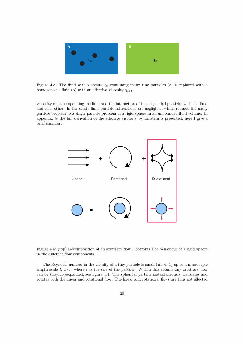
For a suspension of rigid spheres Einstein introduced [19, 20] the effective viscosity, which de-scribes a suspension as a homogeneous Newtonian liquid, see figure 4.3. It incorporates the

27

a b

η0 ηeff

Figure 4.3: The fluid with viscosity η0 containing many tiny particles (a) is replaced with ahomogeneous fluid (b) with an effective viscosity ηeff .

viscosity of the suspending medium and the interaction of the suspended particles with the fluidand each other. In the dilute limit particle interactions are negligible, which reduces the manyparticle problem to a single particle problem of a rigid sphere in an unbounded fluid volume. Inappendix G the full derivation of the effective viscosity by Einstein is presented, here I give abrief summary.

Figure 4.4: (top) Decomposition of an arbitrary flow. (bottom) The behaviour of a rigid spherein the different flow components.

The Reynolds number in the vicinity of a tiny particle is small (Re 1) up to a mesoscopiclength scale L r, where r is the size of the particle. Within this volume any arbitrary flowcan be (Taylor-)expanded, see figure 4.4. The spherical particle instantaneously translates androtates with the linear and rotational flow. The linear and rotational flows are thus not affected

28

r R

V

S

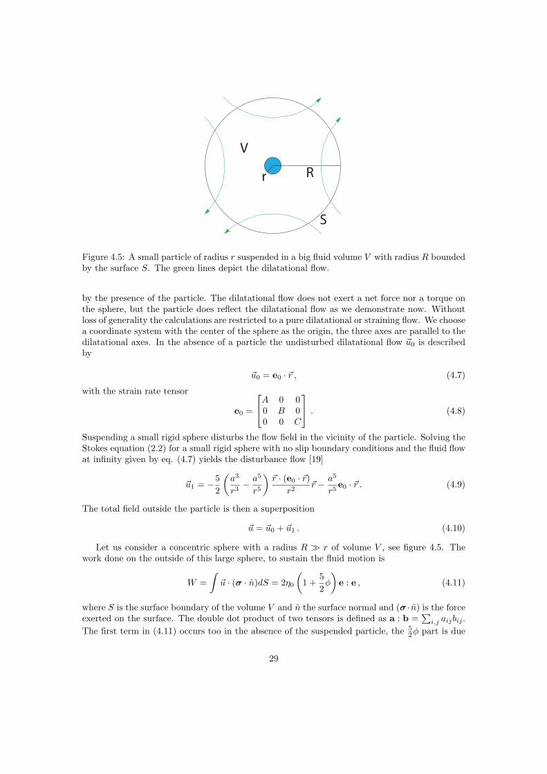
Figure 4.5: A small particle of radius r suspended in a big fluid volume V with radius R boundedby the surface S. The green lines depict the dilatational flow.

by the presence of the particle. The dilatational flow does not exert a net force nor a torque onthe sphere, but the particle does reflect the dilatational flow as we demonstrate now. Withoutloss of generality the calculations are restricted to a pure dilatational or straining flow. We choosea coordinate system with the center of the sphere as the origin, the three axes are parallel to thedilatational axes. In the absence of a particle the undisturbed dilatational flow ~u0 is describedby

~u0 = e0 · ~r , (4.7)

with the strain rate tensor

e0 =

A 0 00 B 00 0 C

. (4.8)

Suspending a small rigid sphere disturbs the flow field in the vicinity of the particle. Solving theStokes equation (2.2) for a small rigid sphere with no slip boundary conditions and the fluid flowat infinity given by eq. (4.7) yields the disturbance flow [19]

~u1 = −52

(a3

r3− a5

r5

)~r · (e0 · ~r)

r2~r − a5

r5e0 · ~r . (4.9)

The total field outside the particle is then a superposition

~u = ~u0 + ~u1 . (4.10)

Let us consider a concentric sphere with a radius R r of volume V , see figure 4.5. Thework done on the outside of this large sphere, to sustain the fluid motion is

W =∫~u · (σ · n)dS = 2η0

(1 +

52φ

)e : e , (4.11)

where S is the surface boundary of the volume V and n the surface normal and (σ · n) is the forceexerted on the surface. The double dot product of two tensors is defined as a : b =

∑i,j aijbij .

The first term in (4.11) occurs too in the absence of the suspended particle, the 52φ part is due

29

to the presence of the particle. The suspension can now be described as a Newtonian fluid withan effective viscosity

ηeff =(

1 +52φ

)η0 . (4.12)

The effective viscosity of a suspension is higher than that of the intrinsic medium. In the case ofsuspensions of passive particles, as considered here, the work done on the outer sphere is equalto the dissipated energy in the volume V . The dilute regime, where this expression is valid andwhere particle interactions are negligible is φ < 2% [4, 41]. The semi dilute regime is definedas 2% < φ < 25% where terms in φ2 become relevant. For small shear rates the spherical cellbody is not expected to deform, therefore a suspension of passive Chlamydomonas is expectedto behave like a suspension of rigid spheres. In the rest of this document the viscosity is denotedas ηeff = (1 +Bφ) η0, for rigid spheres B = 5/2. The effective viscosity in the dilute limit wasfirst derived by Einstein, it is a function only of the intrinsic viscosity of the suspending mediumand the volume fraction of suspended particles.

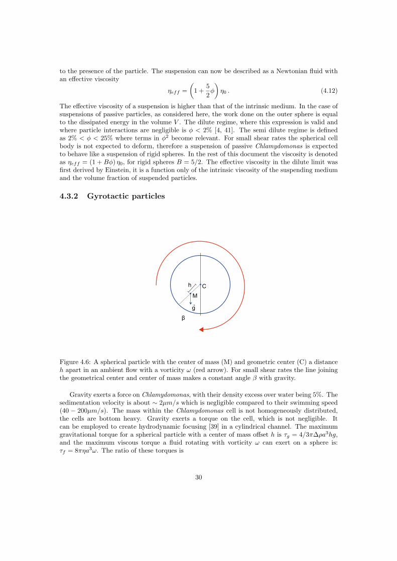
4.3.2 Gyrotactic particles

h

g

β

CM

Figure 4.6: A spherical particle with the center of mass (M) and geometric center (C) a distanceh apart in an ambient flow with a vorticity ω (red arrow). For small shear rates the line joiningthe geometrical center and center of mass makes a constant angle β with gravity.

Gravity exerts a force on Chlamydomonas, with their density excess over water being 5%. Thesedimentation velocity is about ∼ 2µm/s which is negligible compared to their swimming speed(40 − 200µm/s). The mass within the Chlamydomonas cell is not homogeneously distributed,the cells are bottom heavy. Gravity exerts a torque on the cell, which is not negligible. Itcan be employed to create hydrodynamic focusing [39] in a cylindrical channel. The maximumgravitational torque for a spherical particle with a center of mass offset h is τg = 4/3π∆ρa3hg,and the maximum viscous torque a fluid rotating with vorticity ω can exert on a sphere is:τf = 8πηa3ω. The ratio of these torques is

30

λ =τgτf

=∆ρgh6ηω

. (4.13)

Brenner [9] derived an effective viscosity for spherical gyrotactic particles as a function of thisratio in the absence of rotary diffusion

ηeffη0

= 1 + (5/2 + 3/2 sin2 θs(λ))︸︷︷︸B

φ , (4.14)

with

sin θs(λ) =

√12

(1 + λ2)−√

14

(1 + λ2)2 − λ2 sin2 α , (4.15)

where α is the angle between the vorticity vector and gravity. B of eq. (4.14) is plotted in figure4.7 as a function of the dimensionless, inverse shear rate λ and as a function of the shear rateusing Chlamydomonas specific values for the parameters. If gravity and vorticity are parallel,then the gravitational torque has no effect on the effective viscosity and the Einstein formula(4.12) is obtained. Here I consider the case that the angle between vorticity and gravity isα = π/2 and sinα = 1, like in a cone-plate rheometer.

0.0 0.5 1.0 1.5 2.02.0

2.5

3.0

3.5

4.0

λ

B

0.1 0.5 1.0 5.0 10.0 50.0 100.0

2.5

3.0

3.5

4.0

γ

B

.

Figure 4.7: (left) Linear viscosity constant as a function of non-dimensionalised gravitationaltorque. (right) Linear viscosity constant as a function of shear rate using Chlamydomonas specificparameters from [5] & [54]. Gravity is perpendicular to the vorticity of the flow α = π/2).

At small shear rates λ > 1 the gravitational torque balances the viscous torque, see figure4.6. The particles do not rotate at all, the line joining the center of mass and the geometriccenter makes a constant angle with gravity (β). In this limit eq. (4.14) becomes B = 5/2 + 3/2.The first part is due to the reflection of the dilatational field, the 3/2 is due to the reflectionof the rotational field. At higher shear rates λ < 1, the gravitational torque is too small tobalance the viscous torque, and the particles start to rotate with the ambient fluid. For highshear rates λ 1 the gravitational torque becomes negligible compared to the viscous torqueand the Einstein result eq. (4.12) is obtained.

In this case the (effective) diffusion is neglected. It will turn out that compared to the effectiverotary difussion of swimmin suspension the gravitational effect becomes negligible.

31

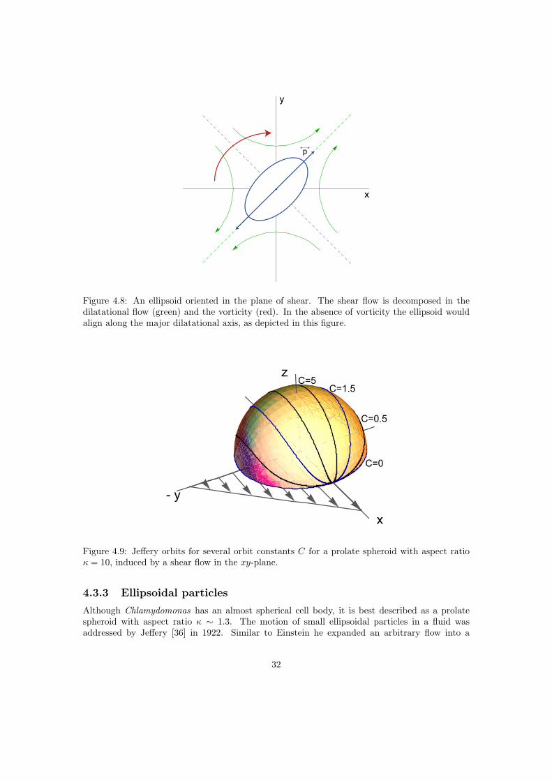
p

x

y

Figure 4.8: An ellipsoid oriented in the plane of shear. The shear flow is decomposed in thedilatational flow (green) and the vorticity (red). In the absence of vorticity the ellipsoid wouldalign along the major dilatational axis, as depicted in this figure.

x

- y

z

C=0

C=0.5

C=1.5C=5

Figure 4.9: Jeffery orbits for several orbit constants C for a prolate spheroid with aspect ratioκ = 10, induced by a shear flow in the xy-plane.

4.3.3 Ellipsoidal particles

Although Chlamydomonas has an almost spherical cell body, it is best described as a prolatespheroid with aspect ratio κ ∼ 1.3. The motion of small ellipsoidal particles in a fluid wasaddressed by Jeffery [36] in 1922. Similar to Einstein he expanded an arbitrary flow into a

32

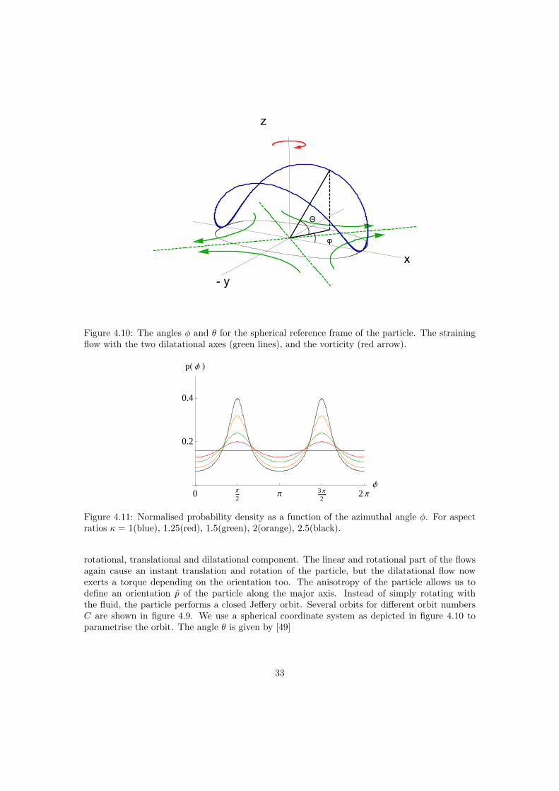
x

- y

z

Θ

φ

Figure 4.10: The angles φ and θ for the spherical reference frame of the particle. The strainingflow with the two dilatational axes (green lines), and the vorticity (red arrow).

0

Π

2Π

3 Π

22 Π

Φ

0.2

0.4

pH Φ L

Figure 4.11: Normalised probability density as a function of the azimuthal angle φ. For aspectratios κ = 1(blue), 1.25(red), 1.5(green), 2(orange), 2.5(black).

rotational, translational and dilatational component. The linear and rotational part of the flowsagain cause an instant translation and rotation of the particle, but the dilatational flow nowexerts a torque depending on the orientation too. The anisotropy of the particle allows us todefine an orientation p of the particle along the major axis. Instead of simply rotating withthe fluid, the particle performs a closed Jeffery orbit. Several orbits for different orbit numbersC are shown in figure 4.9. We use a spherical coordinate system as depicted in figure 4.10 toparametrise the orbit. The angle θ is given by [49]

33

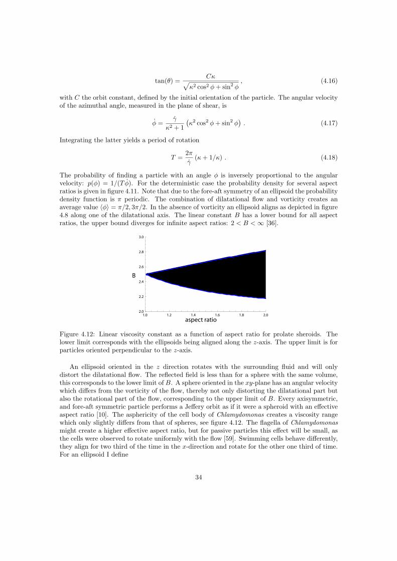
tan(θ) =Cκ√

κ2 cos2 φ+ sin2 φ, (4.16)

with C the orbit constant, defined by the initial orientation of the particle. The angular velocityof the azimuthal angle, measured in the plane of shear, is

φ =γ

κ2 + 1(κ2 cos2 φ+ sin2 φ

). (4.17)

Integrating the latter yields a period of rotation

T =2πγ

(κ+ 1/κ) . (4.18)

The probability of finding a particle with an angle φ is inversely proportional to the angularvelocity: p(φ) = 1/(T φ). For the deterministic case the probability density for several aspectratios is given in figure 4.11. Note that due to the fore-aft symmetry of an ellipsoid the probabilitydensity function is π periodic. The combination of dilatational flow and vorticity creates anaverage value 〈φ〉 = π/2, 3π/2. In the absence of vorticity an ellipsoid aligns as depicted in figure4.8 along one of the dilatational axis. The linear constant B has a lower bound for all aspectratios, the upper bound diverges for infinite aspect ratios: 2 < B <∞ [36].

1.0 1.2 1.4 1.6 1.8 2.02.0

2.2

2.4

2.6

2.8

3.0

aspect ratio

B

Figure 4.12: Linear viscosity constant as a function of aspect ratio for prolate sheroids. Thelower limit corresponds with the ellipsoids being aligned along the z-axis. The upper limit is forparticles oriented perpendicular to the z-axis.

An ellipsoid oriented in the z direction rotates with the surrounding fluid and will onlydistort the dilatational flow. The reflected field is less than for a sphere with the same volume,this corresponds to the lower limit of B. A sphere oriented in the xy-plane has an angular velocitywhich differs from the vorticity of the flow, thereby not only distorting the dilatational part butalso the rotational part of the flow, corresponding to the upper limit of B. Every axisymmetric,and fore-aft symmetric particle performs a Jeffery orbit as if it were a spheroid with an effectiveaspect ratio [10]. The asphericity of the cell body of Chlamydomonas creates a viscosity rangewhich only slightly differs from that of spheres, see figure 4.12. The flagella of Chlamydomonasmight create a higher effective aspect ratio, but for passive particles this effect will be small, asthe cells were observed to rotate uniformly with the flow [59]. Swimming cells behave differently,they align for two third of the time in the x-direction and rotate for the other one third of time.For an ellipsoid I define

34

τ =t(φ = π

4 →3π4 )

t(φ = 3π4 →

5π4 )

(4.19)

as the ratio of alignment time and tumbling time, where φ denotes the angle as in eq. 4.17.

τ =π − 2ArcCot(κ)

2ArcCot(κ). (4.20)

The experimental value τ ∼ 2 corresponds to an effective aspect ratio κe = 1.7. In section 4.4.2the theoretical work of Jones et al. [37] is discussed who showed that the beating flagella in com-bination with a spherical cell body creates an effective ratio of κe = 1.1. The actual value of Bdepends on the average orientation of the particles, this is addressed in section 4.5. The aspher-ical cell body of Chlamydomonas creates a small deviation in the effective viscosity comparedto perfect spheres: B = 2.5 ± 0.1, the effective aspect ratio of swimming cells creates a slightlybigger deviation: B = 2.5 ± 0.3. The shape of the particle has a small effect on the effectiveviscosity, which depends on the average orientation of the particles. The latter is addressed insection 4.5.

Based on the separate analysis of the influence of asphericity and gravity, the viscosity of asuspension of non-swimming Chlamydomonas is best described as the viscosity of a suspensionof rigid spheres. At small shear rates (λ 0) gravity enhances the viscosity.

4.4 Rheology of dilute suspensions of swimming Chlamy-domonas

In this section I present two new derivations of the influence of swimming of Chlamydomonas onthe effective viscosity of the suspension.

4.4.1 Three-point-force model

Chlamydomonas has an almost spherical cell body, which serves as a motivation to model it as arigid spherical particle with radius a which creates an additional flow due to swimming. Recallthat the latter is described by a superposition of three stokeslets, see eq. (3.3). Using the sameapproach as in section 4.3 for passive spheres, the work done on the surface of a large sphericalvolume containing the particle is compared to the same fluid volume containing a homogeneousfluid. This volume is large compared to the size of the particle. A surface integral over this volumeor a volume average will not depend on the near field, but rather on the far field behaviour. Herea brief summary of the derivation of the effective viscosity is given, the full derivation is providedin appendix G. By substituting the multipole expansion

1|~r − ~r1|

=1r

+~r1 · ~rr3

+O(r−5) . (4.21)

in equation (3.4) the far field is obtained as (see appendix D)

~us = − 38πη

rS : (r ⊗ r)

r2. (4.22)

with the stresslet tensor being

35

S = S (p⊗ p− I/3) , (4.23)

where p denotes the swimming direction of the cell. The stresslet strength S = bF2 depends on

position and magnitude of the point forces, see figure 4.13, and it changes during the swimmingstroke. During the major part of the stroke Chlamydomonas is a puller (S > 0), for the minorpart of the effective stroke, where the effective flagellar forces are behind the centerline of the cellbody, it is a pusher (S < 0). As viscosity experiments typically last several seconds, the stressletstrength denotes the average over a beat cyce S = 〈S〉t. The magnitude of S can be derivedfrom the flows and swimming speed. The positions of the point forces in the flows of figure 3.4provide the dipole length b. With the linear relation between force and velocity for low Reynoldsnumbers and considering the cell as a sphere with radius a, the dipole force is calculated fromF = 6πηa〈U〉. Throughout this chapter a value 〈U〉 = 40µm/s is used [59]. The total flow is asuperposition of the applied flow, the reflected flow and the swimming induced flow:

~u = ~u0 + ~u1 + ~us . (4.24)

Evaluating the work done on a big sphere containing the microswimmer in order to sustain themotion (G.5) yields

W

V η0=(

1 +52φ

)e : e +

n

VS : e . (4.25)

with n the number density of swimmers. By substituting S = bF/2 = 3bπηrU this is recasted as

W

V η0=(

1 +52φ

)e : e +

94φb

a

U

a(< p⊗ p > −I/3) : e . (4.26)

where 〈...〉 denotes the ensemble average over both particle orientation and time and φ is thevolume fraction of suspended particles. The ⊗ symbol denotes the dyadic, tensor or Kroneckerproduct. In this case the work done on the outer sphere is not equal to the dissipated energywithin the fluid volume. The dissipation in the system is given by eq. (4.25) with an additionalterm ∼ S : S. The the cell metabolism leads to a dissipation too, but it is not taken into accounthere. The liquid crystal order parameter Q = 〈p⊗ p〉 − I/3 is used in the rest of the document.A cone-plate rheometer measures the viscosity as η = σxy/exy. The effective viscosity is givenby

ηeffη0

= 1 +52φ+

94φb

a

U

aγQxy , (4.27)

where is used that exy = γ/2, see eq. (4.6). This is in agreement with literature[54]. Thedisadvantage of this derivation is that it is mathematically laborious. It does not provide anynew information therefore it is better to use a volume average approach. Using the volumeaverage approach of Landau and Lifschitz [41] another new derivation of the effective viscosityof a suspension of Chlamydomonas is derived. The full derivation is presented in appendix H,here again a brief summary. The stress tensor is averaged over a large volume

〈σ〉 =1V

∫σdV , (4.28)

which is decomposed in a pressure, strain and particle dependent term as

〈σ〉 = −〈p〉I + 2η0〈e〉+ n〈Sparticle〉 , (4.29)

36

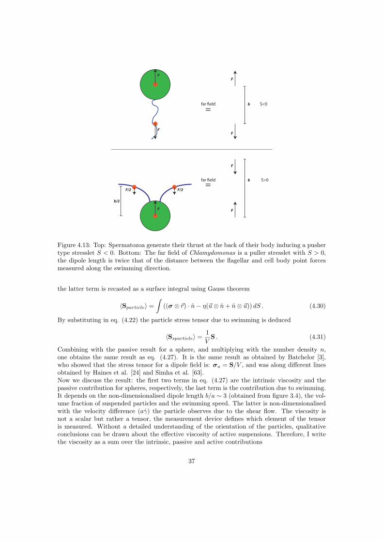
F

F

F

F/2 F/2

=

F

F

F

F

far eld

=far eld

S<0

S>0

b/2

b

b

Figure 4.13: Top: Spermatozoa generate their thrust at the back of their body inducing a pushertype stresslet S < 0. Bottom: The far field of Chlamydomonas is a puller stresslet with S > 0,the dipole length is twice that of the distance between the flagellar and cell body point forcesmeasured along the swimming direction.

the latter term is recasted as a surface integral using Gauss theorem

〈Sparticle〉 =∫

((σ ⊗ ~r) · n− η(~u⊗ n+ n⊗ ~u)) dS . (4.30)

By substituting in eq. (4.22) the particle stress tensor due to swimming is deduced

〈Ssparticle〉 =1V

S . (4.31)

Combining with the passive result for a sphere, and multiplying with the number density n,one obtains the same result as eq. (4.27). It is the same result as obtained by Batchelor [3],who showed that the stress tensor for a dipole field is: σa = S/V , and was along different linesobtained by Haines et al. [24] and Simha et al. [63].Now we discuss the result: the first two terms in eq. (4.27) are the intrinsic viscosity and thepassive contribution for spheres, respectively, the last term is the contribution due to swimming.It depends on the non-dimensionalised dipole length b/a ∼ 3 (obtained from figure 3.4), the vol-ume fraction of suspended particles and the swimming speed. The latter is non-dimensionalisedwith the velocity difference (aγ) the particle observes due to the shear flow. The viscosity isnot a scalar but rather a tensor, the measurement device defines which element of the tensoris measured. Without a detailed understanding of the orientation of the particles, qualitativeconclusions can be drawn about the effective viscosity of active suspensions. Therefore, I writethe viscosity as a sum over the intrinsic, passive and active contributions

37

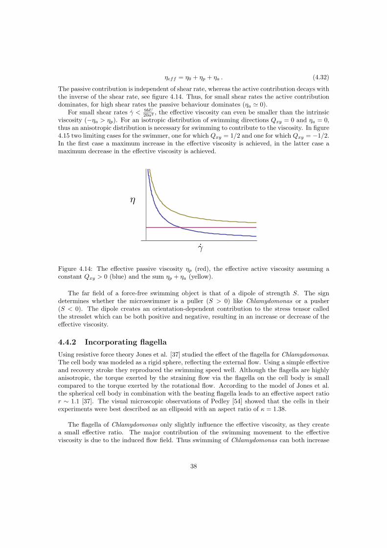
ηeff = η0 + ηp + ηa . (4.32)

The passive contribution is independent of shear rate, whereas the active contribution decays withthe inverse of the shear rate, see figure 4.14. Thus, for small shear rates the active contributiondominates, for high shear rates the passive behaviour dominates (ηa ' 0).

For small shear rates γ < 9bU20a2 , the effective viscosity can even be smaller than the intrinsic

viscosity (−ηa > ηp). For an isotropic distribution of swimming directions Qxy = 0 and ηa = 0,thus an anisotropic distribution is necessary for swimming to contribute to the viscosity. In figure4.15 two limiting cases for the swimmer, one for which Qxy = 1/2 and one for which Qxy = −1/2.In the first case a maximum increase in the effective viscosity is achieved, in the latter case amaximum decrease in the effective viscosity is achieved.

γ

η

Figure 4.14: The effective passive viscosity ηp (red), the effective active viscosity assuming aconstant Qxy > 0 (blue) and the sum ηp + ηa (yellow).

The far field of a force-free swimming object is that of a dipole of strength S. The signdetermines whether the microswimmer is a puller (S > 0) like Chlamydomonas or a pusher(S < 0). The dipole creates an orientation-dependent contribution to the stress tensor calledthe stresslet which can be both positive and negative, resulting in an increase or decrease of theeffective viscosity.

4.4.2 Incorporating flagella

Using resistive force theory Jones et al. [37] studied the effect of the flagella for Chlamydomonas.The cell body was modeled as a rigid sphere, reflecting the external flow. Using a simple effectiveand recovery stroke they reproduced the swimming speed well. Although the flagella are highlyanisotropic, the torque exerted by the straining flow via the flagella on the cell body is smallcompared to the torque exerted by the rotational flow. According to the model of Jones et al.the spherical cell body in combination with the beating flagella leads to an effective aspect ratior ∼ 1.1 [37]. The visual microscopic observations of Pedley [54] showed that the cells in theirexperiments were best described as an ellipsoid with an aspect ratio of κ = 1.38.

The flagella of Chlamydomonas only slightly influence the effective viscosity, as they createa small effective ratio. The major contribution of the swimming movement to the effectiveviscosity is due to the induced flow field. Thus swimming of Chlamydomonas can both increase

38

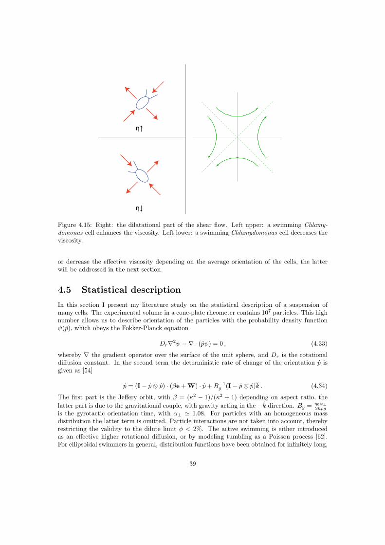
η↑

η↓

Figure 4.15: Right: the dilatational part of the shear flow. Left upper: a swimming Chlamy-domonas cell enhances the viscosity. Left lower: a swimming Chlamydomonas cell decreases theviscosity.

or decrease the effective viscosity depending on the average orientation of the cells, the latterwill be addressed in the next section.

4.5 Statistical description

In this section I present my literature study on the statistical description of a suspension ofmany cells. The experimental volume in a cone-plate rheometer contains 107 particles. This highnumber allows us to describe orientation of the particles with the probability density functionψ(p), which obeys the Fokker-Planck equation

Dr∇2ψ −∇ · (pψ) = 0 , (4.33)

whereby ∇ the gradient operator over the surface of the unit sphere, and Dr is the rotationaldiffusion constant. In the second term the deterministic rate of change of the orientation p isgiven as [54]

p = (I− p⊗ p) · (βe + W) · p+B−1g (I− p⊗ p)k . (4.34)

The first part is the Jeffery orbit, with β = (κ2 − 1)/(κ2 + 1) depending on aspect ratio, thelatter part is due to the gravitational couple, with gravity acting in the −k direction. Bg = η0α⊥

2hρgis the gyrotactic orientation time, with α⊥ ' 1.08. For particles with an homogeneous massdistribution the latter term is omitted. Particle interactions are not taken into account, therebyrestricting the validity to the dilute limit φ < 2%. The active swimming is either introducedas an effective higher rotational diffusion, or by modeling tumbling as a Poisson process [62].For ellipsoidal swimmers in general, distribution functions have been obtained for infinitely long,

39

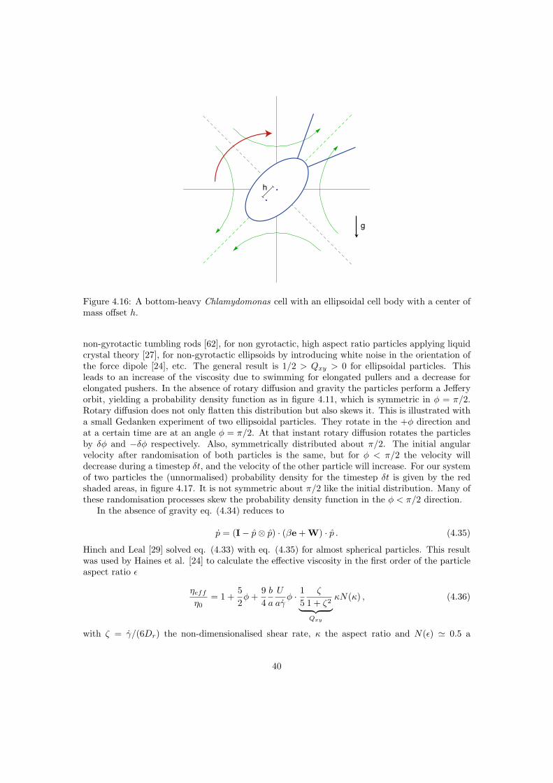
g

h

Figure 4.16: A bottom-heavy Chlamydomonas cell with an ellipsoidal cell body with a center ofmass offset h.

non-gyrotactic tumbling rods [62], for non gyrotactic, high aspect ratio particles applying liquidcrystal theory [27], for non-gyrotactic ellipsoids by introducing white noise in the orientation ofthe force dipole [24], etc. The general result is 1/2 > Qxy > 0 for ellipsoidal particles. Thisleads to an increase of the viscosity due to swimming for elongated pullers and a decrease forelongated pushers. In the absence of rotary diffusion and gravity the particles perform a Jefferyorbit, yielding a probability density function as in figure 4.11, which is symmetric in φ = π/2.Rotary diffusion does not only flatten this distribution but also skews it. This is illustrated witha small Gedanken experiment of two ellipsoidal particles. They rotate in the +φ direction andat a certain time are at an angle φ = π/2. At that instant rotary diffusion rotates the particlesby δφ and −δφ respectively. Also, symmetrically distributed about π/2. The initial angularvelocity after randomisation of both particles is the same, but for φ < π/2 the velocity willdecrease during a timestep δt, and the velocity of the other particle will increase. For our systemof two particles the (unnormalised) probability density for the timestep δt is given by the redshaded areas, in figure 4.17. It is not symmetric about π/2 like the initial distribution. Many ofthese randomisation processes skew the probability density function in the φ < π/2 direction.

In the absence of gravity eq. (4.34) reduces to

p = (I− p⊗ p) · (βe + W) · p . (4.35)

Hinch and Leal [29] solved eq. (4.33) with eq. (4.35) for almost spherical particles. This resultwas used by Haines et al. [24] to calculate the effective viscosity in the first order of the particleaspect ratio ε

ηeffη0

= 1 +52φ+

94b

a

U

aγφ · 1

5ζ

1 + ζ2︸︷︷︸Qxy

κN(κ) , (4.36)

with ζ = γ/(6Dr) the non-dimensionalised shear rate, κ the aspect ratio and N(ε) ' 0.5 a

40

rotation

Π/2-∆ Π/2+∆

0 Π

2Π

Φ

0.2

0.4

0.6

0.8

pH Φ L

rotation

0 Π

2Π

Φ

0.2

0.4

0.6

0.8

pH Φ L

Figure 4.17: Left: Deterministc probability density for a prolate spheroid (black line). The redarea is the not normalised probability density function of two particles. Right: Deterministicprobability density for a prolate spheroid (black line) and the probability density incorporatingrotary diffusion.

geometric function. An aspect ratio r = 1.3 is used throughout this section. The avera georientation of the particles is due to competition between the applied flow and rotary diffusion.In figure 4.18 eq. (4.36) is plotted using both the passive Dr = 0.001/s and two values for theactive rotary diffusion Dr = 0.4/s [35] & Dr = 0.13/s [54]. For γ > γc the passive contributiondominates, for lower shear rates the viscosity is enhanced, reaching a plateau for small shear rates.γ < Dr. The zero shear rate limit for the active part of the viscosity is limγ→0 ηa/η0 ∼ U

aDr

0.1 0.5 1.0 5.0 10.0 50.0 100.0

3

4

5

6

7

shear rate γ (1/s)

η eff/η

0-1

.

Dr=0.4/s

Dr=0.001/s

Dr=0.13/s

Figure 4.18: The effective viscosity as a function of shear rate in a log-linear plot for three valuesof the rotary diffusion constant and the assymptotic behaviour for high shear rates (purple line).

A general analytic solution for eqs. (4.33) & (4.34) is not known, but for weak flows γ 1/Bg ∼ 0.3 /s a solution was obtained analytically by Pedley et al. [54] in the first order ofε = Bgω. They calculated the stress tensor incorporating all possible shape, gravitational andflow influences, see appendix E, which is linear in the applied shear flow. This results in shear-independent viscosity for small shear rates, which is in good approximation given by

limγ1/Bg

ηeffη0

= 1 + 2.6φ+9BgU

4aφf(Dr, Bg) , (4.37)

41

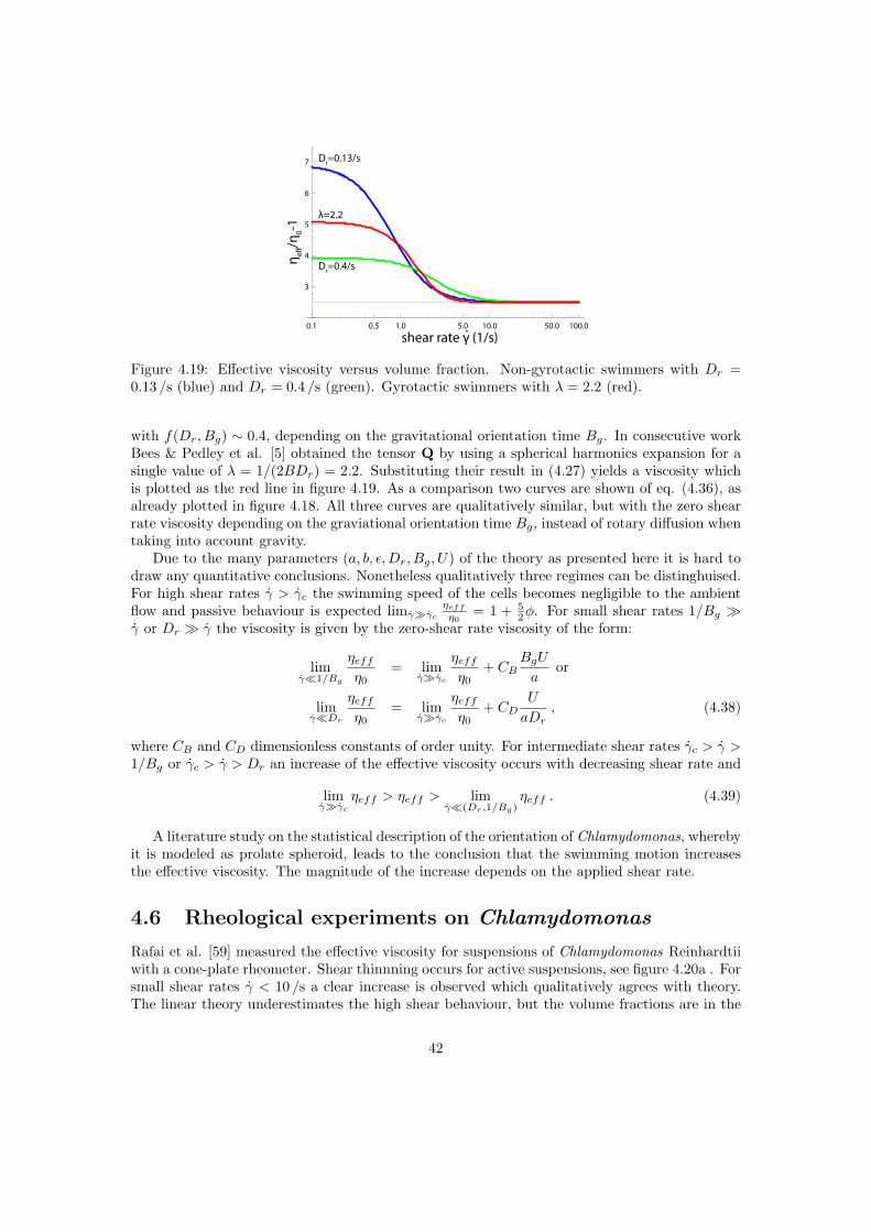
0.1 0.5 1.0 5.0 10.0 50.0 100.0

3

4

5

6

7

shear rate γ (1/s)

η eff/η

0-1

.

Dr=0.4/s

Dr=0.13/s

λ=2.2

Figure 4.19: Effective viscosity versus volume fraction. Non-gyrotactic swimmers with Dr =0.13 /s (blue) and Dr = 0.4 /s (green). Gyrotactic swimmers with λ = 2.2 (red).

with f(Dr, Bg) ∼ 0.4, depending on the gravitational orientation time Bg. In consecutive workBees & Pedley et al. [5] obtained the tensor Q by using a spherical harmonics expansion for asingle value of λ = 1/(2BDr) = 2.2. Substituting their result in (4.27) yields a viscosity whichis plotted as the red line in figure 4.19. As a comparison two curves are shown of eq. (4.36), asalready plotted in figure 4.18. All three curves are qualitatively similar, but with the zero shearrate viscosity depending on the graviational orientation time Bg, instead of rotary diffusion whentaking into account gravity.

Due to the many parameters (a, b, ε,Dr, Bg, U) of the theory as presented here it is hard todraw any quantitative conclusions. Nonetheless qualitatively three regimes can be distinghuised.For high shear rates γ > γc the swimming speed of the cells becomes negligible to the ambientflow and passive behaviour is expected limγγc

ηeff

η0= 1 + 5

2φ. For small shear rates 1/Bg γ or Dr γ the viscosity is given by the zero-shear rate viscosity of the form:

limγ1/Bg

ηeffη0

= limγγc

ηeffη0

+ CBBgU

aor

limγDr

ηeffη0

= limγγc

ηeffη0

+ CDU

aDr, (4.38)

where CB and CD dimensionless constants of order unity. For intermediate shear rates γc > γ >1/Bg or γc > γ > Dr an increase of the effective viscosity occurs with decreasing shear rate and

limγγc

ηeff > ηeff > limγ(Dr,1/Bg)

ηeff . (4.39)

A literature study on the statistical description of the orientation of Chlamydomonas, wherebyit is modeled as prolate spheroid, leads to the conclusion that the swimming motion increasesthe effective viscosity. The magnitude of the increase depends on the applied shear rate.

4.6 Rheological experiments on Chlamydomonas

Rafai et al. [59] measured the effective viscosity for suspensions of Chlamydomonas Reinhardtiiwith a cone-plate rheometer. Shear thinnning occurs for active suspensions, see figure 4.20a . Forsmall shear rates γ < 10 /s a clear increase is observed which qualitatively agrees with theory.The linear theory underestimates the high shear behaviour, but the volume fractions are in the

42

Figure 4.20: a) The effective viscosity as a function of the shear rate for 4 different volumefractions of living Chlamydomonas and the suspending medium. b) The effective viscosity ofa suspension of active (living) and inactive (dead) Chlamydomonas, as a function of volumefraction. Taken from [59].

Table 4.1

Linear effective viscosity constant B for γ = 5 /srigid spheres 2.5ellipsoid r=1.3 2.4-2.6ellispoid r=1.7 2.2-2.8gyrotactic spheres 2.6Haines 2.8Pedley 2.9

semi-dilute regime in which the theory is not expected to be valid anymore. Both suspensionsof active and inactive particles show an increase of the viscosity with respect to the viscosity ofthe suspending medium η0 for a shear rate γ = 5 /s see figure 4.20b . Theoretical predictions forthe linear coefficient at this shear rate are listed in table 4.1.

Only small deviations of the spherical value are to be expected. Due to the high scatteringand very few data points for active and passive suspensions for low volume fractions φ < 5%,no conclusion can be drawn about the difference between active and passive suspensions. Thetheory as presented in the last section can thus not be tested.

For higher volume fractions the difference between active and passive suspensions is clear,both displaying a nonlinear increase. The active suspension shows the biggest increase. Theresults were fitted using the Krieger-Dougherty relation [40]

ηeffη0

=(

1− φ

φmax

)−φmaxB

, (4.40)

where φmax the maximum packing fraction set to the maximum random packing fraction 0.62[59]. B is used as a fitting parameter giving B = 2.5 ± 0.1 and B = 4.5 ± 0.2 for inactive andactive suspensions respectively. Linear theory underestimates the experimental results for non-dilute volume fractions. The big difference for higher volume fractions indicates that higher order

43

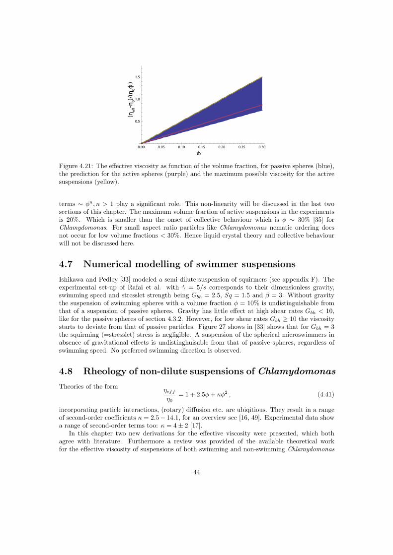
0.00 0.05 0.10 0.15 0.20 0.25 0.30

0.5

1.0

1.5

ф

(ηef

f-η0)/

(η0ф

)

Figure 4.21: The effective viscosity as function of the volume fraction, for passive spheres (blue),the prediction for the active spheres (purple) and the maximum possible viscosity for the activesuspensions (yellow).

terms ∼ φn, n > 1 play a significant role. This non-linearity will be discussed in the last twosections of this chapter. The maximum volume fraction of active suspensions in the experimentsis 20%. Which is smaller than the onset of collective behaviour which is φ ∼ 30% [35] forChlamydomonas. For small aspect ratio particles like Chlamydomonas nematic ordering doesnot occur for low volume fractions < 30%. Hence liquid crystal theory and collective behaviourwill not be discussed here.

4.7 Numerical modelling of swimmer suspensions

Ishikawa and Pedley [33] modeled a semi-dilute suspension of squirmers (see appendix F). Theexperimental set-up of Rafai et al. with γ = 5/s corresponds to their dimensionless gravity,swimming speed and stresslet strength being Gbh = 2.5, Sq = 1.5 and β = 3. Without gravitythe suspension of swimming spheres with a volume fraction φ = 10% is undistinguishable fromthat of a suspension of passive spheres. Gravity has little effect at high shear rates Gbh < 10,like for the passive spheres of section 4.3.2. However, for low shear rates Gbh ≥ 10 the viscositystarts to deviate from that of passive particles. Figure 27 shows in [33] shows that for Gbh = 3the squirming (=stresslet) stress is negligible. A suspension of the spherical microswimmers inabsence of gravitational effects is undistinghuisable from that of passive spheres, regardless ofswimming speed. No preferred swimming direction is observed.

4.8 Rheology of non-dilute suspensions of Chlamydomonas

Theories of the formηeffη0

= 1 + 2.5φ+ κφ2 , (4.41)

incorporating particle interactions, (rotary) diffusion etc. are ubiqitious. They result in a rangeof second-order coefficients κ = 2.5− 14.1, for an overview see [16, 49]. Experimental data showa range of second-order terms too: κ = 4± 2 [17].

In this chapter two new derivations for the effective viscosity were presented, which bothagree with literature. Furthermore a review was provided of the available theoretical workfor the effective viscosity of suspensions of both swimming and non-swimming Chlamydomonas

44

cells. The only available experimental results were conducted at a high shear rate at which thedifference in effective viscosity of active and inactive suspensions is negligible.

45

Chapter 5

Conclusion & discussion

Microscopic behaviour of a single cell: Based on an analysis of the cell architecture anew hypothesis for the flagellar synchronisation was formulated. The two flagella are connectedboth via the basal body and the distal striated fiber. It is not unlikely that this coupling hasa bigger effect on synchronisation than hydrodynamic interactions. This might be investigatedby modelling the flagella as two driven oscillators connected by a Hookean spring. Also, thecoupling through the mutual connection to the cell body, which can rotate and translate, couldbe responsible for the observed synchronisation. Again, this might be modeled by using twodriven oscillators which are connected to a spherical cell body which can rotate and translate, astarting point could be the analysis of the coupled clocks of Huygens [6].

On the microscopic scale of a single Chlamydomonas cell the analytic three-point-force modelwas extended with a qualitative analysis of the flagellar stroke to incorporate the movement ofthe flagella. A simple effective and recovery stroke was derived, where the forces are exertedparallel to the swimming direction. The flow field is a superposition of three stokeslets. A com-parision was made with the experiments of Guasto et al. [23] on Chlamydomonas swimming ina thin film. The latter is best described as a 2D fluid, therefore the 2D stokeslet was used. Thefull details of the flow field are reproduced during both the effective and recovery stroke.

Macroscopic rheology: On a macroscopic scale the effective viscosity of a dilute suspen-sion of Chlamydomonas has been addressed. For immotile cells the almost spherical cell bodyleads to a viscosity like for a suspension of passive rigid spheres. At low shear rates (> 1/s) thegravitational couple increases the viscosity. Two new derivations have been presented for the ef-fective viscosity of a dilute suspension of swimming Chlamydomonas cells. One along the theoryof Einstein, the other based on the volume average approach of Landau & Lifshitz. Both resultsare in agreement with literature. The effective viscosity depends on the average orientation ofthe cells. Based on a literature study, three regimes can be determined. For low shear rates theviscosity is described by the zero shear rate viscosity which is higher than for a suspension ofpassive particles due to the puller type swimming and the elongated body shape. For intermedi-ate shear rates the viscosity decreases with shear rate. For high shear rates an active suspensionbehaves like a passive suspension of rigid spheres. This theory is valid for dilute suspensionsφ < 2% where particle interactions are negligible. The high number of parameters of the theory

46

requires simultaneous analysis of the following cell properties:

• Size and aspect ratio of the particles;

• Swimming speed;

• Dipole length;

• Rotational diffusion;

• Centre of mass offset.

Many of these parameters not only differ among different strains, but also among cells of thesame population. The swimming speed, dipole length and rotational diffusion depend on theenvironmental conditions too.

The single experiment on the viscosity of suspensions of swimming Chlamydomonas of Rafaiet al. [59] was conducted at high shear rate where the difference between swimming and non-swimming suspensions is small. Due to the very few scattered data points in the dilute limit,no conclusion can be drawn on the validity of the theory at this shear rate. Experiments at lowshear rates should reveal a larger difference. Theories incorporating higher order contributions(φn) for simple passive systems do exist but show a wide variety of results. It is not to beexpected that for the more complex active systems theories for volume fractions of more than2% will have any validity.

The interference of the flagellar movement and the applied shear flow not yet clear. It mightaffect the swimming orientation of the cells. The underlying problem is that, although theflagellar movement is well recorded, the internal ’algorithm’ or switching mechanism responsiblefor the beating pattern remains a mystery. This is an interesting field of research in itself.

47

Appendix A

Acknowledgment

First of all I like to thank Paul for giving me the chance to go abroad for my master project, andfor the interesting (Skype-)discussions we had, and Holger to allow me to spend a year in hisgroup. It was not an easy year, therefore I like to thank all the people who have knowingly andunknowingly supported me throughout this period. All the group members of the AG Stark, Ilike to thank all of you for the year I spend with you, and in particular Sujin and Andreas for thenumerous discussions about my subject and for correcting my thesis. The support of my parentswas essential for getting this thesis finished, thank you a lot! I like to thank the departmentof Applied Physics at the TU Eindhoven, and explicitly Thijs Michels, Henk Swagten, GerritKroese, Ton van Leeuwen, I still owe all of you a beer at the ”Borrel”. Special thanks goes out toIgnacio for helping me out when I got stuck with tensor calculus and for the nice discussions wehad both about physical and non-physical subjects. Finally, I like to thank all the members ofmy graduation committe for taking the time to work their way through my master thesis: KeesStorm en Rob van der Heijden.

48

Appendix B

Technology assessment

With the current focus on algae as a basis for feed, coatings, hydrogen producer, etc. it is evidentthat a deeper understanding of both microscopic and macroscopic properties of suspensions ofChlamydomonas is necessary. An application of the rheological theory would be for motilitymeasurements. First the number density of swimmers has to be obtained. Chlamydomonas hasa slight density excess over water, by measuring the mass density of the suspension the massfraction of Chlamydomonas is obtained. The mass of a single cell is known, thus the numberdensity can be calculated. The motility can then be measured by measuring the viscosity, for ex-ample with a rheometer. The viscosity-motility relation can for dilute suspension be determinedanalytically, but for higher suspensions a semi-empirical approach will be more usefull. Thistechnique is not limited to Chlamydomonas, but could also be used in hospitals to determine themotility quality of human spermatozoa.

49

Appendix C

Hydrodynamics

Incompressible fluid dynamics is described by the Navier-Stokes equation

ρ

(∂~u

∂t+ ~u · ∇~u

)= −∇p+ η∇2~u+ ~F , (C.1)

with ~F the external body forces and ρ and η the density and viscosity of the fluid respectively. Letus consider a submerged object of size L translating with speed U . The Navier-Stokes equationeq. (C.1) can then be nondimensionalised by using the object speed and size, the viscosity andthe density of the fluid. With

~u = U~u′∂∂t = U

L∂∂t′

∇ = ∇′L

p = ηULL2 p

′

~F = ηULL3

~F ′

(C.2)

eq. (C.1) can be recasted as

ρUL

η

(∂~u′

∂t′+ ~u′ · ∇′~u′

)= −∇′p′ + (∇′)2~u′ + ~F ′ . (C.3)

The prefactor ρULη is the Reynolds number (Re). For Re 1 the Navier-Stokes equation reduces

to the Stokes equation−∇p+ η∇2~u = ~F . (C.4)

This is a time indepedent equation, the fluid flow at any moment in time is uniquely defined bythe boundary conditions. A force monopole at the origin is mathematically described as

−∇p+ η∇2~u = ~Fδ(r) , (C.5)

which can be solved by using e.g. Greens function theory to give the Stokeslet solution

~uSto(~r) = T(~r) · ~F , T(~r) =1

8πηr

(I +

~r ⊗ ~rr2

), (C.6)

with I the unit tensor and ⊗ the tensorial or Kronecker product. A force dipole of strength S isa superposition of two point forces ~F and −~F a length b apart and induces a stresslet

~us = − 38πη

S : (r ⊗ r)r2

r , (C.7)

50

with p the unit vector along the line joining the points at which the two point forces are exerted.The stresslet tensor is

S = S (p⊗ p− I/3) . (C.8)

Eq. (C.7) can be derived by taking the limit of two stokeslets of strength F for vanishing distanced between the acting point forces but remaining a constant S = Fd. Eq. (C.7) can be recastedas

~us = − S

8πη1− 3(p · r)2

r2r , (C.9)

with 1− 3(p · r)2 = 1− 3 cos2 θ = P2(cos θ), where P2(x) is the second Legendre polynom. In thesame manner a quadrupole with direction along the unit vector p at the origin with strength Qinduces (in leading order) a source doublet field

~uSD(~r) =Q

4πηr3

(I/3− ~r ⊗ ~r

r2

)· p . (C.10)

The aforementioned flow fields are obtained for an unbound fluid volume in 3D. Certain thinfilms show (quasi-)2D behaviour. Solving eq. (C.4) for a point force in 2D yields the 2D stokeslet

~uSto2D(~r) = T(~r) · ~F , T(~r) =1

4πη

(−ln(r/r0)I +

~r ⊗ ~rr2

). (C.11)

where r0 is an arbitrary length scale. Let us consider two point forces exerted in oppositedirection. The first at the origin, the second at a point ~r1. The flow field is then described as

~uSto2D(~r) =F

4πη

([−ln(r/r0) + ln(|r − ~r1|/r0)]I +

~r ⊗ ~rr2− (~r − ~r1)⊗ (~r − ~r1)

r2

). (C.12)

and can be rewritten as

~uSto2D(~r) =F

4πη

(ln(|r − ~r1|/r)I +

~r ⊗ ~rr2− (~r − ~r1)⊗ (~r − ~r1)

r2

). (C.13)

A derivation of these flow fields is given in the book of Pozrikidis [56]. Along the same lines thetwo dimensional stresslet can be derived

~uStr2D =1

4πηr(1− 2(p · r)2)r . (C.14)

This result can be obtained by a multipole expansion of two stokeslets using

ln(r

r − r1) = 0− ~r1 · ~r

r2. (C.15)

The stresses exerted on a submerged particle can be integrated over the particle surface to givethe total force, dipole strength and quadrupole strength

~F =∫

σ · ndA , (C.16)

p′I + S + R =∫~r ⊗ (σ · n)dA , (C.17)

Q =∫~r ⊗ (~r ⊗ (σ · n))dA . (C.18)

51

The dipole strength is decomposed in an isotropic p′I, a symmetric stresslet S and an antisym-metric rotlet or couplet R term

p′I =∫

13~r · σ · nIdA , (C.19)

S =∫ [

12

(~r ⊗ (σ · n) + (σ · n)⊗ ~r))− 13~r · σ · nI− η(~u⊗ n+ n⊗ ~u)

]dA , (C.20)

R =∫

12

(~r ⊗ (σ · n)− (σ · n)⊗ ~r)dA . (C.21)

This decomposition was introduced by Batchelor [3]. The last term in the stresslet is zero for arigid particle, but by adding this term the integral can be taken over any fluid volume containingone particle. The rotlet can be restated as

R =12ε : τ , (C.22)

with τ the torque on the particle and ε the Levi-Civita permutation tensor. Batchelor [3] showedthat the contribution to the stress by the presence of the particle is as follows

σp =S + RV

. (C.23)

52

Appendix D

Three-point-force model

The velocity field due to a distribution of point forces is a superposition of stokeslets

~u(~r) =∑i

T(~r − ~ri) · ~Fi , (D.1)

where ~Fi being a point force at position ri and

T(~r) =1

8πηr

(I +

r ⊗ rr2

), (D.2)

the Oseen tensor. Chlamydomonas with its two flagella is modeled as a superposition of threepoint forces, one at its body centre which we define as the origin. (0, 0, F ) at ~r0 = (0, 0, 0)and two point forces in the xz plane: (0, 0,−F/2) at ~r1,2 = (±a, 0, b/2). The flow due to thesuperposition of these forces is given

~u(~r) = ~F ·Tsum(~r) , (D.3)

with

8πη ·Tsum(~r) =1r

(I +

~r ⊗ ~rr2

)− 1

21

|~r − ~r1|

(I +

(~r − ~r1)⊗ (~r − ~r1)|~r − ~r1|2

)(D.4)

−12

1|~r − ~r2|

(I +

(~r − ~r2)⊗ (~r − ~r2)|~r − ~r2|2

). (D.5)

The multipole expansion for r1 r

1|~r − ~r1|

=1r

+~r1 · ~rr3

+O(r−5) , (D.6)

is used to deduce the I part of eq. (D.5)

I(

1r− 1

21

|~r − ~r1|− 1

21

|~r − ~r2|

)= −1

2(~r1 + ~r2) · ~r

r3I (D.7)

Again by using a multipole expansion

1|~r − ~r1|3

=1r3

+3~r1 · ~rr5

+O(r−7) (D.8)

53

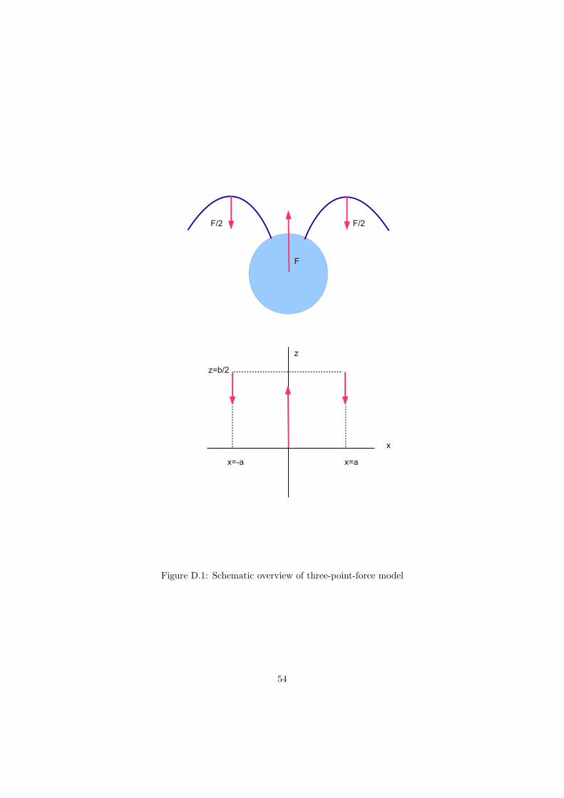
x

z

x=ax=-a

z=b/2

F

F/2F/2

Figure D.1: Schematic overview of three-point-force model

54

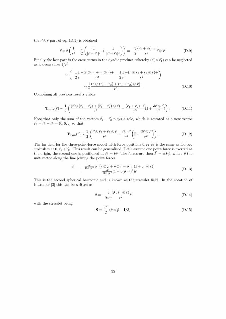
the ~r ⊗ ~r part of eq. (D.5) is obtained

~r ⊗ ~r(

1r3− 1

2

(1

|~r − ~r1|3+

1|~r − ~r2|3

))= −3

2(~r1 + ~r2) · ~r

r5~r ⊗ ~r . (D.9)

Finally the last part is the cross terms in the dyadic product, whereby (~r1⊗ ~r1) can be neglectedas it decays like 1/r3

∼(−1

21r

−(r ⊗ r1 + r1 ⊗ r)+r2

− 12

1r

−(r ⊗ r2 + r2 ⊗ r)+r2

)∼ 1

2(r ⊗ (r1 + r2) + (r1 + r2)⊗ r)

r3. (D.10)

Combining all previous results yields

Tsum(~r) ∼ 12

((~r ⊗ (~r1 + ~r2) + (~r1 + ~r2)⊗ ~r)

r3− (~r1 + ~r2) · ~r

r3(I +

3~r ⊗ ~rr2

)). (D.11)

Note that only the sum of the vectors ~r1 + ~r2 plays a role, which is restated as a new vector~r3 = ~r1 + ~r2 = (0, 0, b) so that

Tsum(~r) ∼ 12

(~r ⊗ ~r3 + ~r3 ⊗ ~r

r3− ~r3 · ~r

r3

(I +

3~r ⊗ ~rr2

)). (D.12)

The far field for the three-point-force model with force positions 0, ~r1, ~r2 is the same as for twostokeslets at 0, ~r1 +~r2. This result can be generalised. Let’s assume one point force is exerted atthe origin, the second one is positioned at ~r3 = bp. The forces are then ~F = ±F p, where p theunit vector along the line joining the point forces.

~u = bF16πηr2 p · (r ⊗ p+ p⊗ r − p · r (I + 3r ⊗ r))

= bF16πηr2 (1− 3(p · r)2)r

(D.13)

This is the second spherical harmonic and is known as the stresslet field. In the notation ofBatchelor [3] this can be written as

~u = − 38πη

S : (r ⊗ r)r2

r (D.14)

with the stresslet being

S =bF

2(p⊗ p− I/3) (D.15)

55

Appendix E

Stress tensor

For a Newtonian fluid the stress tensor is

σ = −pI + 2ηe . (E.1)

The so called ’Batchelor stresses’ due to the presence of an ellipsoidal particle are [3]

σp = 4ηnv [α1E : 〈pppp〉+ α2(E · 〈pp〉+ 〈pp〉 ·E) + α3E + α4E : 〈pp〉I]

+n

2

[ε · 〈~L〉+

12α0〈(p× ~L)p+ p(p× ~L)〉

], (E.2)

where ~L = −ρvhp× ~g is the gravitational torque for a body of volume v, gravity offset h and ~ggravity acceleration. The functions αi depend the aspect ratio, and ε is the alternating tensor.The short hand notation for the Kronecker product is used ~a ⊗ ~b = ~a~b and 〈..〉 denotes theensemble average. Rotary diffusion leads to a stress given by

σd = 2ηnvDrα5(〈p⊗ p〉 − I/3) . (E.3)

The swimming of an object yields

σs = S(〈p⊗ p〉 − I/3) . (E.4)

Combining the previous equations leads to a total stress

σ = −p+ 2ηe + σp + σs + σd . (E.5)

The diffusive and swimming term can be combined [29]

σsd = (S + 2ηnvα5Dr)(〈p⊗ p〉 − I/3) . (E.6)

The ratio of swimming and diffusion term is

β =6πηaUb2ηvDrα5

∼ 103 . (E.7)

For passive rotary diffusion β ∼ 103 and for active rotary diffusion β ∼ 50. At small shear ratesε = Bω 1 the stress tensor has been derived analytically [54] in the first order of the strainrate as

σxy,p + σxy,sd =η0φγα⊥

8

(9η0Uhρga

b

a(J2 − 2α0J5) + 2.6

), (E.8)

56

where their constant αF = 1. α0 ∼ 0.3 is the aspect ratio minus one and α⊥ ∼ 7 a constantwhich depends on aspect ratio. Ji = Ji(λ) are functions of the parameter λ = (2BDr)−1.

The linear viscosity coefficient is then

B =(ηeffη0− 1)/φ =

9η0α⊥U8hρga

b

a(J2 − 2α0J5) + 2.6 . (E.9)

The latter term (J2 − 2α0J5) ∼ 0.4 for λ = 2.2 [54].

57

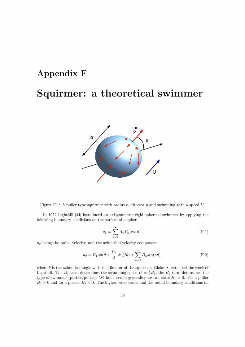
Appendix F

Squirmer: a theoretical swimmer

U

p

θ2r

Puller Pusher

Figure F.1: A puller type squirmer with radius r, director p and swimming with a speed U .

In 1952 Lighthill [44] introduced an axisymmetric rigid spherical swimmer by applying thefollowing boundary conditions on the surface of a sphere

ur =∞∑n=1

AnPn(cos θ) , (F.1)

ur being the radial velocity, and the azimuthal velocity component

uθ = B1 sin θ +B2

2sin(2θ) +

∞∑n=3

Bnsin(nθ) , (F.2)

where θ is the azimuthal angle with the director of the squirmer. Blake [8] extended the work ofLighthill. The B1-term determines the swimming speed U = 2

3B1, the B2 term determines thetype of swimmer (pusher/puller). Without loss of generality we can state B1 > 0. For a pullerB2 > 0 and for a pusher B2 < 0. The higher order terms and the radial boundary conditions do

58

not change this general behaviour and are thus neglected (Am = Bn = 0 for n > 2 and m > 0).For a single squirmer in a non-moving Newtonian fluid the velocity is obtained by solving theStokes equation

ur = −23B1 cos(θ) +

23B1

(ar

)3

P1(cos(θ)) +((a

r

)4

−(ar

)2)B2P2(cos(θ)) , (F.3)

where Pn(x) denotes the n-th Legendre polynomial i.e. P1(x) = x, P2(x) = 12 (3x2 − 1). The

azimuthal velocity component is

uθ =23B1 sin(θ) +

B1

3

(ar

)3

V1(cos(θ)) +12

(ar

)4

B2V2(cos(θ)) , (F.4)

where V1(cos(θ)) = sin(θ) and V2(cos(θ)) = sin(θ) cos(θ). Setting r = a one easily sees that thisobeys the boundary conditions. The swimming speed is related to the first coefficient U = 2

3B1.The induced flow field can also be restated as:

~us = B1

(ar

)3(p · ~rrr − p

3

)+((a

r

)4

−(ar

)2)B2P2

(p · ~rr

)r +

(ar

)4

B2p · ~rr

(p · ~rr− p)

(F.5)The far field (up to 1/r2) for a squirmer is a stresslet, the radial velocity component is

ur = −23B1 cos(θ)−

(ar

)2

B2P2(cos(θ)) . (F.6)

and the azimuthal component is

uθ =23B1 sin(θ) . (F.7)

59

Appendix G

Einstein derivation of theeffective viscosity of a suspensionof Chlamydomonas

For dilute suspensions particle interactions are negligible, the many particle problem therebyreduces to a single particle problem. Any arbitrary flow can be decomposed in a rotational,dilatational and linear component. A spherical particle instanteneously rotate and translatewith the ambient fluid, but will affect the dilatational part of the flow. The latter is denoted as

~u0 = e0 · ~r , (G.1)

with the strain rate tensor

e0 =

A 0 00 B 00 0 C

. (G.2)

Incompressibility of the flow (∇ · ~u) requires Trace(e0) = 0. The particle reflects the flow viathe no-slip boundary conditions, leading to a distortion field:

~u1 = −52

(a3

r3− a5

r5

)~r · (e0 · ~r)

r2~r +

a5

r5e0 · ~r . (G.3)

The total field outside the particle is then:

~u = ~u0 + ~u1 . (G.4)

The work done on a large fluid volume containing the particle is compared with the same fluidvolume containing a homogeneous liquid. The work on a sphere in a fluid volume V can becalculated by taking the following surface integral over the boundary of the fluid volume:

W =∫

(σ · n) · ~udS , (G.5)

where S is the surface boundary of the volume V and n the surface normal and (σ · n) is the forceexerted on the surface. The volume V is chosen to be a cocentric infinitely large sphere. With

60

σ ∼ U/r,∫dS ∼ r2 and u0 ∼ r, in this case only the terms in u1 ∼ 1/r2 give a contribution

in the first order of the volume fraction. To obtain the result for many suspended particles theintegral is evaluated and multiplied with the number density of suspended particles

W

V= 2η0

(1 +

12φ

)e0 : e0 , (G.6)

with φ the volume fraction of suspended particles. The double dot product of two tensorsis defined as a : b =

∑i,j aibi. Due to the presence of the particles the volume average strain

tensor is modified too. Taking the volume average over the same volume V gives

e =1V

∫12

(∇+∇T )~udV = e0 +1V

∫∇~u1dV = (1− φ)e0 . (G.7)

Substituting in eq. (G.6) yields

W

V= 2η0

1 + 12φ

(1− φ)2e : e . (G.8)

If the volume would contain a homogeneous fluid the work on the sphere would be described by

W

V= 2ηeffe : e . (G.9)

Introducing the effective viscosity ηeff allows us to treat the suspension as a homogeneous fluid

ηeffη0

=1 + 1

2φ

(1− φ)2' 1 +

52φ , (G.10)

For a microswimmer the effective viscosity will be derived along the same lines as for the passivesphere. The far field of any swimming force-free organism or object is a stresslet field, of strength

D =bF

16πη. (G.11)

~us = −Dr2

(1− 3 cos2 θ)r . (G.12)

The total flow field is a superposition of the applied shear flow, the disturbance flow due tothe presence of the particle and the swimmer stresslet flow

~u = ~ushear + ~usph + ~us(p) , (G.13)

The mechanical work on a large fluid volume containing the particle is

W = c

∫r→∞

(σ · n) · ~udS . (G.14)

And the correction in the strain rate is given as

E∗ = E− c∫∇ · ~udU = E− c

∫r→∞

~u

r· ndS . (G.15)

A dilatational flow field with the axis of the cartesian coordinate system coinciding with the 3dilatational directions is described by ~ushear = E · ~r, with

E =

A 0 00 B 00 0 C

. (G.16)

61

In leading order the stress tensor of stresslet has two non-zero terms in spherical coordinates

σs =

σs,rr σs,rθ 00 0 00 0 0

, (G.17)

whereby σs,rr = ηD 2(1−3 cos2 θ)r3 and σs,rθ = ηD (−3 sin θ cos θ)

2r3 . The terms in eq. (G.14) involvingonly passive contributions were calculated in section 4.4. The only two terms involving theswimmer flow that give a contriubtion in the first order of φ are

W1 =n

U

∫(σs,rrushear,r + σs,θushear,θ)dS , (G.18)

leading toW1

ηU=

35Dφ

a

(~p⊗ ~p− I

3

): E . (G.19)

Combining with the Einstein result of eq. (G.6) yields the total work on the sphere

Wtotal

ηU=(

1 +φ

2

)E : E +

35Dφ

a

(~p⊗ ~p− I

3

): E . (G.20)

The second integral eq. (G.15) involving the correction of the strain rate is given by

E∗ = E(1− φ)−R · φDa

β ·RT = E(1− φ) +65Dφ

a

(~p⊗ ~p− I

3

). (G.21)

The double dot product of the strain can then be recasted as

E : E =E∗ : E∗

(1− φ)2+

125

φD

a(1− φ)2

(~p⊗ ~p− I

3

)E∗ +O(φ2) . (G.22)

Substituting this result in eq. (G.20) yields the total work on the sphere as a function of theactual strain rate

Wtotal

ηV =(

1 + φ2

)(E∗:E∗

(1−φ)2 + 125

φDa(1−φ)2

(~p⊗ ~p− I

3

))E∗

+ 35

Dφa(1−φ)

(~p⊗ ~p− I

3

):(E∗ + 6

5Dφa

(~p⊗ ~p− I

3

)).

(G.23)

This can be expanded in first order of φ to give

Wtotal

ηV=(

1 +52φ

)E∗ : E∗ + 3

φD

a

(~p⊗ ~p− I

3

): E∗ . (G.24)

The work on the sphere depends on the swimming orientation with respect to the applied shearflow. In e.g. a cone-plate rheometer the shear viscosity is measured. For a simple shear flow thestrain rate tensor is:

E∗ =

0 γ 00 0 00 0 0

. (G.25)

The measured viscosity is deduced from eq. (G.24)

ηeffη0

=(

1 +52φ

)+ 3

φD

γapxpy . (G.26)

Combining with eq. (G.12) yields the effective viscosity in first order of the volume fraction fora spherical microswimmer

ηeffη0

= 1 +(

52

+94b

a

U

aγpxpy

)φ . (G.27)

62

Appendix H

Volume average effective viscosityof a suspension ofChlamydomonas

The volume average method of Landau & Lifshitz [41] is briefly presented here, first for passivespheres, later on for microswimmers. In the dilute limit the many particle problem reduces to asingle particle suspended in an unbound dilatational flow ~u = E ·~r. The stress tensor is averagedover a big sphere V containing the small particle

〈σ〉 =1V

∫σdV , (H.1)

This expression can be restated as

〈σ〉 = −〈p〉I + η0 (∇〈~u〉+ (∇〈~u〉)T )︸︷︷︸2〈E〉

+∫V

(σ − η0(∇~u+ (∇~u)T ) + pI

)dV . (H.2)

The first terms two terms denote the Newtonian behaviour of the fluid outside the particle, thelatter integral is a measure of the internal stress within the rigid sphere. It is strictly zero withinthe fluid. The analysis of the internal stresses within the particle is possible, but it is simpler toconvert the volume integral into a surface integral by using the identitie

σ = ∇ · (σ ⊗ ~r) , (H.3)

and the theorem of Gauss ∫(∇ · F)dV =

∫F · ndS , (H.4)∫

(∇F)dV =∫

F⊗ ndS . (H.5)

The volume integral in eq. (H.2) is then recasted as∫S

((σ ⊗ ~r) · n− η(~u⊗ n+ n⊗ ~u)) dS , (H.6)

63

where is S the surface boundary of the volume V . The pressure term in the integral drops out.Note that this equation is linear in the velocity ~u and is the same as the stresslet of Batchelor(C.20) except for the uninteresting isotropic part. Thus this integral can be calculated over boththe surface of the particle, but it is often easier to choose a large volume containing a smallparticle. The solution of the integral for tiny rigid spheres is given in [41], using this result tocalculate the part in eq. (H.2) involving the strain rate yields

〈σ〉 = η0〈E〉+ η052φ〈E〉 . (H.7)

Substitution of eq. (G.7) yields

〈σ〉 = η0〈E〉+ η052

φ

1− φ〈E〉 ' η0

(1 +

52φ

)〈E〉 . (H.8)

This is the same result as obtained by Einstein. Let us now consider the volume average stresstensor for a microswimmer. As eq. (H.6) is linear in the velocity we can simply add the extracontribution of the swimmer induced field. From now on the unit vector is denoted as n = r.Any force-free microswimmer induces a stresslet in the far field

~u = − S

4πη0r2P2(p · r)r = −D

r2P2(p · r)r , (H.9)

and the pressure given by

p = −ηDr3P2(p · r) . (H.10)

Velocity gradients occur in eq. (H.6), using the identities ∇~r = I, ∇r = r,∇r = 1/r(I− r ⊗ r),∇(1/r2) = −2r/r2 the gradient of the stresslet field is obtained

∇~u = −Dr2

[−2

P2(p · r)r3

r ⊗ r +P2(p · r)

r3(I− r ⊗ r) + r

∇P2(p · r)r2

], (H.11)

with∇P2(p · r) =

1r

3(p · r)p · (I− r ⊗ r) =1r

3(p · r)(p− (p · r)r)⊗ r . (H.12)

Combining these expressions to calculate the symmetric gradient

∇~u+(∇~u)T = −Dr2

[−2r ⊗ r + P2(p · r)(I− r ⊗ r) + 3(p · r)

(12

(p⊗ r + p⊗ r))− 3(p · r)r ⊗ r

].

(H.13)The first part of eq. (H.6) can thus be written as

−Dr2

[−2r ⊗ r + 2P2(p · r)r ⊗ r +

32

(p · r)(p⊗ r + p⊗ r)− (p · r)r ⊗ r], (H.14)

where (I · r)⊗ r = r ⊗ r and [(r ⊗ r) · r]⊗ r = r ⊗ r is used. The second part of the integral ineq. (H.6) is

−η(~u⊗ n+ n⊗ ~u) =Dη0r2

2P2(p · r)r ⊗ r . (H.15)

Combining the latter two expressions eq. (H.6) reads

−Dη0r2

∫ [−2r ⊗ r + 3(p · r)

(12

(p⊗ r + p⊗ r))]

dΩ , (H.16)

64

The integral involves the orientation of the microswimmer p, it is independent of the applied flowfield. The only second rank tensors that give a non-zero symmetric contribution by averagingover the unit sphere are I and p⊗ p. Thus it is clear that

〈σ〉 = AI +Bp⊗ p . (H.17)

The trace of the tensor is Trace(σ) = 3A+B. Taking the inproduct with p⊗ p yields∫(AI +Bp⊗ p) : (p⊗ p)dΩ = A+B . (H.18)

The latter part of eq. (H.16) is zero when averaged over the unit sphere. With∫(r ⊗ r) : (p⊗ p)dΩ =

8π3. (H.19)

and Trace( ˆr ⊗ r) = 0 the two constants A and B can be determined, yielding a contribution tothe stress:

4πη0D(p⊗ p− I/3) . (H.20)

So that〈σ〉 = η0〈E〉+ η0

52φ〈E〉+ S(〈p⊗ p〉 − I/3) . (H.21)

with S the stresslet strength.

65

Bibliography

[1] Bruce Alberts, Alexander Johnson, Julian Lewis, Martin Raff, Keith Roberts, and PeterWalter. Molecular Biology of the Cell. Garland Science, 5 edition, November 2007.

[2] G. Alexander and J. Yeomans. Hydrodynamic Interactions at Low Reynolds Number. Ex-perimental Mechanics, 50(9):1283–1292, November 2010.

[3] G. K. Batchelor. The stress system in a suspension of force-free particles. Journal of FluidMechanics, 41(03):545–570, 1970.

[4] G. K. Batchelor and G. K. Batchelor. An Introduction to Fluid Dynamics. CambridgeUniversity Press, February 2000.

[5] M. A. Bees, N. A. Hill, and T. J. Pedley. Analytical approximations for the orientationdistribution of small dipolar particles in steady shear flows. Journal of Mathematical Biology,36(3):269–298, February 1998.

[6] Matthew Bennett, Michael F. Schatz, Heidi Rockwood, and Kurt Wiesenfeld. Huygens’sclocks. Proceedings of the Royal Society of London. Series A: Mathematical, Physical andEngineering Sciences, 458(2019):563–579, March 2002.

[7] J. Blake and A. Chwang. Fundamental singularities of viscous flow. Journal of EngineeringMathematics, 8(1):23–29, January 1974.

[8] J. R. Blake. A spherical envelope approach to ciliary propulsion. Journal of Fluid Mechanics,46(01):199–208, 1971.

[9] H. Brenner. Rheology of a dilute suspension of dipolar spherical particles in an externalfield. Journal of Colloid and Interface Science, 32(1):141–158, January 1970.

[10] F. P. Bretherton. The motion of rigid particles in a shear flow at low Reynolds number.Journal of Fluid Mechanics, 14(02):284–304, 1962.

[11] C. J. Brokaw. Flagellar movement: a sliding filament model. Science (New York, N.Y.),178(60):455–462, November 1972.

[12] C. J. Brokaw. Thinking about flagellar oscillation. Cell motility and the cytoskeleton,66(8):425–436, August 2009.

[13] C. J. Brokaw and D. J. L. Luck. Bending patterns of chlamydomonas flagella I. Wild-typebending patterns. Cell Motility, 3(2):131–150, 1983.

[14] Sebastien Camalet and Frank Julicher. Generic aspects of axonemal beating. New Journalof Physics, 2(1):24+, October 2000.

66

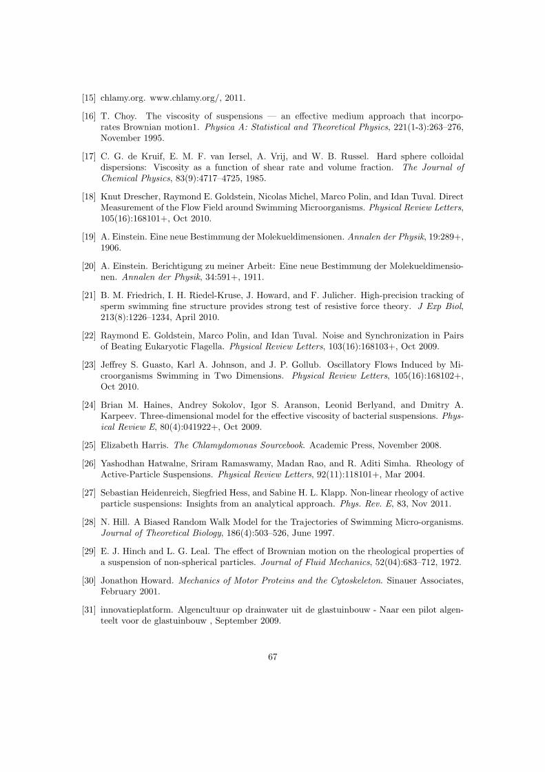
[15] chlamy.org. www.chlamy.org/, 2011.

[16] T. Choy. The viscosity of suspensions — an effective medium approach that incorpo-rates Brownian motion1. Physica A: Statistical and Theoretical Physics, 221(1-3):263–276,November 1995.

[17] C. G. de Kruif, E. M. F. van Iersel, A. Vrij, and W. B. Russel. Hard sphere colloidaldispersions: Viscosity as a function of shear rate and volume fraction. The Journal ofChemical Physics, 83(9):4717–4725, 1985.

[18] Knut Drescher, Raymond E. Goldstein, Nicolas Michel, Marco Polin, and Idan Tuval. DirectMeasurement of the Flow Field around Swimming Microorganisms. Physical Review Letters,105(16):168101+, Oct 2010.

[19] A. Einstein. Eine neue Bestimmung der Molekueldimensionen. Annalen der Physik, 19:289+,1906.

[20] A. Einstein. Berichtigung zu meiner Arbeit: Eine neue Bestimmung der Molekueldimensio-nen. Annalen der Physik, 34:591+, 1911.

[21] B. M. Friedrich, I. H. Riedel-Kruse, J. Howard, and F. Julicher. High-precision tracking ofsperm swimming fine structure provides strong test of resistive force theory. J Exp Biol,213(8):1226–1234, April 2010.

[22] Raymond E. Goldstein, Marco Polin, and Idan Tuval. Noise and Synchronization in Pairsof Beating Eukaryotic Flagella. Physical Review Letters, 103(16):168103+, Oct 2009.

[23] Jeffrey S. Guasto, Karl A. Johnson, and J. P. Gollub. Oscillatory Flows Induced by Mi-croorganisms Swimming in Two Dimensions. Physical Review Letters, 105(16):168102+,Oct 2010.

[24] Brian M. Haines, Andrey Sokolov, Igor S. Aranson, Leonid Berlyand, and Dmitry A.Karpeev. Three-dimensional model for the effective viscosity of bacterial suspensions. Phys-ical Review E, 80(4):041922+, Oct 2009.

[25] Elizabeth Harris. The Chlamydomonas Sourcebook. Academic Press, November 2008.

[26] Yashodhan Hatwalne, Sriram Ramaswamy, Madan Rao, and R. Aditi Simha. Rheology ofActive-Particle Suspensions. Physical Review Letters, 92(11):118101+, Mar 2004.

[27] Sebastian Heidenreich, Siegfried Hess, and Sabine H. L. Klapp. Non-linear rheology of activeparticle suspensions: Insights from an analytical approach. Phys. Rev. E, 83, Nov 2011.

[28] N. Hill. A Biased Random Walk Model for the Trajectories of Swimming Micro-organisms.Journal of Theoretical Biology, 186(4):503–526, June 1997.

[29] E. J. Hinch and L. G. Leal. The effect of Brownian motion on the rheological properties ofa suspension of non-spherical particles. Journal of Fluid Mechanics, 52(04):683–712, 1972.

[30] Jonathon Howard. Mechanics of Motor Proteins and the Cytoskeleton. Sinauer Associates,February 2001.

[31] innovatieplatform. Algencultuur op drainwater uit de glastuinbouw - Naar een pilot algen-teelt voor de glastuinbouw , September 2009.

67

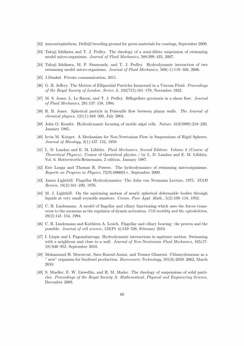
[32] innovatieplatform. Delfzijl breeding ground for green materials for coatings, September 2009.

[33] Takuji Ishikawa and T. J. Pedley. The rheology of a semi-dilute suspension of swimmingmodel micro-organisms. Journal of Fluid Mechanics, 588:399–435, 2007.

[34] Takuji Ishikawa, M. P. Simmonds, and T. J. Pedley. Hydrodynamic interaction of twoswimming model micro-organisms. Journal of Fluid Mechanics, 568(-1):119–160, 2006.

[35] J.Dunkel. Private communication, 2011.

[36] G. B. Jeffery. The Motion of Ellipsoidal Particles Immersed in a Viscous Fluid. Proceedingsof the Royal Society of London. Series A, 102(715):161–179, November 1922.

[37] M. S. Jones, L. Le Baron, and T. J. Pedley. Biflagellate gyrotaxis in a shear flow. Journalof Fluid Mechanics, 281:137–158, 1994.

[38] R. B. Jones. Spherical particle in Poiseuille flow between planar walls. The Journal ofchemical physics, 121(1):483–500, July 2004.

[39] John O. Kessler. Hydrodynamic focusing of motile algal cells. Nature, 313(5999):218–220,January 1985.

[40] Irvin M. Krieger. A Mechanism for Non-Newtonian Flow in Suspensions of Rigid Spheres.Journal of Rheology, 3(1):137–152, 1959.

[41] L. D. Landau and E. M. Lifshitz. Fluid Mechanics, Second Edition: Volume 6 (Course ofTheoretical Physics). Course of theoretical physics / by L. D. Landau and E. M. Lifshitz,Vol. 6. Butterworth-Heinemann, 2 edition, January 1987.

[42] Eric Lauga and Thomas R. Powers. The hydrodynamics of swimming microorganisms.Reports on Progress in Physics, 72(9):096601+, September 2009.

[43] James Lighthill. Flagellar Hydrodynamics: The John von Neumann Lecture, 1975. SIAMReview, 18(2):161–230, 1976.

[44] M. J. Lighthill. On the squirming motion of nearly spherical deformable bodies throughliquids at very small reynolds numbers. Comm. Pure Appl. Math., 5(2):109–118, 1952.

[45] C. B. Lindemann. A model of flagellar and ciliary functioning which uses the forces trans-verse to the axoneme as the regulator of dynein activation. Cell motility and the cytoskeleton,29(2):141–154, 1994.

[46] C. B. Lindemann and Kathleen A. Lesich. Flagellar and ciliary beating: the proven and thepossible. Journal of cell science, 123(Pt 4):519–528, February 2010.

[47] I. Llopis and I. Pagonabarraga. Hydrodynamic interactions in squirmer motion: Swimmingwith a neighbour and close to a wall. Journal of Non-Newtonian Fluid Mechanics, 165(17-18):946–952, September 2010.

[48] Mohammad H. Morowvat, Sara Rasoul-Amini, and Younes Ghasemi. Chlamydomonas as a” new” organism for biodiesel production. Bioresource Technology, 101(6):2059–2062, March2010.

[49] S. Mueller, E. W. Llewellin, and H. M. Mader. The rheology of suspensions of solid parti-cles. Proceedings of the Royal Society A: Mathematical, Physical and Engineering Science,December 2009.

68

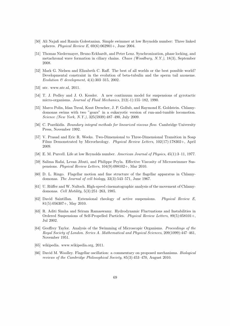
[50] Ali Najafi and Ramin Golestanian. Simple swimmer at low Reynolds number: Three linkedspheres. Physical Review E, 69(6):062901+, June 2004.

[51] Thomas Niedermayer, Bruno Eckhardt, and Peter Lenz. Synchronization, phase locking, andmetachronal wave formation in ciliary chains. Chaos (Woodbury, N.Y.), 18(3), September2008.

[52] Mark G. Nielsen and Elizabeth C. Raff. The best of all worlds or the best possible world?Developmental constraint in the evolution of beta-tubulin and the sperm tail axoneme.Evolution & development, 4(4):303–315, 2002.

[53] ntr. www.ntr.nl, 2011.

[54] T. J. Pedley and J. O. Kessler. A new continuum model for suspensions of gyrotacticmicro-organisms. Journal of Fluid Mechanics, 212(-1):155–182, 1990.

[55] Marco Polin, Idan Tuval, Knut Drescher, J. P. Gollub, and Raymond E. Goldstein. Chlamy-domonas swims with two ”gears” in a eukaryotic version of run-and-tumble locomotion.Science (New York, N.Y.), 325(5939):487–490, July 2009.

[56] C. Pozrikidis. Boundary integral methods for linearized viscous flow. Cambridge UniversityPress, November 1992.

[57] V. Prasad and Eric R. Weeks. Two-Dimensional to Three-Dimensional Transition in SoapFilms Demonstrated by Microrheology. Physical Review Letters, 102(17):178302+, April2009.

[58] E. M. Purcell. Life at low Reynolds number. American Journal of Physics, 45(1):3–11, 1977.

[59] Salima Rafai, Levan Jibuti, and Philippe Peyla. Effective Viscosity of Microswimmer Sus-pensions. Physical Review Letters, 104(9):098102+, Mar 2010.

[60] D. L. Ringo. Flagellar motion and fine structure of the flagellar apparatus in Chlamy-domonas. The Journal of cell biology, 33(3):543–571, June 1967.

[61] U. Ruffer and W. Nultsch. High-speed cinematographic analysis of the movement of Chlamy-domonas. Cell Motility, 5(3):251–263, 1985.

[62] David Saintillan. Extensional rheology of active suspensions. Physical Review E,81(5):056307+, May 2010.

[63] R. Aditi Simha and Sriram Ramaswamy. Hydrodynamic Fluctuations and Instabilities inOrdered Suspensions of Self-Propelled Particles. Physical Review Letters, 89(5):058101+,Jul 2002.

[64] Geoffrey Taylor. Analysis of the Swimming of Microscopic Organisms. Proceedings of theRoyal Society of London. Series A. Mathematical and Physical Sciences, 209(1099):447–461,November 1951.

[65] wikipedia. www.wikipedia.org, 2011.

[66] David M. Woolley. Flagellar oscillation: a commentary on proposed mechanisms. Biologicalreviews of the Cambridge Philosophical Society, 85(3):453–470, August 2010.

69

Documents

Eindhoven University of Technology MASTER Chlamydomonas