EIGENMODES OF ISOSPECTRAL DRUMS∗

TOBIN A. DRISCOLL†

SIAM REV. c© 1997 Society for Industrial and Applied MathematicsVol. 39, No. 1, pp. 1–17, March 1997 001

Abstract. Recently it was proved that there exist nonisometric planar regions that have identicalLaplace spectra. That is, one cannot “hear the shape of a drum.” The simplest isospectral regionsknown are bounded by polygons with reentrant corners. While the isospectrality can be provenmathematically, analytical techniques are unable to produce the eigenvalues themselves. Further-more, standard numerical methods for computing the eigenvalues, such as adaptive finite elements,are highly inefficient. Physical experiments have been performed to measure the spectra, but theaccuracy and flexibility of this method are limited. We describe an algorithm due to Descloux andTolley [Comput. Methods Appl. Mech. Engrg., 39 (1983), pp. 37–53] that blends singular finite el-ements with domain decomposition and show that, with a modification that doubles its accuracy,this algorithm can be used to compute efficiently the eigenvalues for polygonal regions. We presentresults accurate to 12 digits for the most famous pair of isospectral drums, as well as results foranother pair.

Key words. eigenvalues, elliptic operators, isospectrality, finite-element methods, domain de-composition, method of particular solutions

AMS subject classifications. 65N25, 35P99, 35Q60

PII. S0036144595285069

1. Introduction. In 1966 Mark Kac [12] posed the question, “Can one hear theshape of a drum?” He was referring to the problem of whether the Laplacian operatorwith Dirichlet boundary conditions could have identical spectra on two distinct planarregions. Recently Gordon, Webb, and Wolpert [11] answered the question negativelyvia an elegantly constructed counterexample, justifiably attracting a great deal ofattention [7, 8, 15]. The simplest form of their example is a pair of regions boundedby eight-sided polygons, henceforth called the GWW isospectral drums; see Figure 1.1.Numerous similar examples have since been discovered [5].

The simplest and most versatile proof of isospectrality employs “transplanta-tion” [4] of the eigenfunctions. The regions are shown to be (or are constructed to be)made up of nonoverlapping translations, rotations, and reflections of a single shape,such as a triangle. Given an eigenfunction on one region, one can prescribe a func-tion over the other region whose values over each piece are linear combinations of theeigenfunction values over several of the pieces of the first region. The combinationsare chosen to satisfy the boundary conditions and to match values and derivativesat interfaces between pieces, and the interior equation is satisfied by superposition.Hence the result is an eigenfunction of the second region having the same eigenvalue.To complete the proof of isospectrality, one need only check that the procedure isinvertible. Note that the proof is nonconstructive and other information, particularlythe actual values of the eigenvalues, remains unknown.

To find the eigenvalues, it is natural to turn to numerical computation. However,straightforward numerical procedures for computing the eigenvalues [14] are ineffi-cient because of the presence of reentrant corners. Even an adaptive approach, suchas Bank’s PLTMG [3], obtains very slow convergence for the eigenvalue estimates.

∗Received by the editors April 24, 1995; accepted for publication (in revised form) March 13,1996. This work was supported by DOE grant DE-FG02-94ER25199.

http://www.siam.org/journals/sirev/39-1/28506.html†Center for Applied Mathematics, Cornell University, Ithaca, NY 14853 (driscoll@na-

net.ornl.gov).

1

2 TOBIN A. DRISCOLL

-3 -2 -1 0 1 2 3-3

-2

-1

0

1

2

3

-3 -2 -1 0 1 2 3-3

-2

-1

0

1

2

3

FIG. 1.1. The GWW isospectral drums and subdivisions used for the domain decompositionmethod.

Another well-known technique for eigenvalue problems, the method of particular so-lutions [10], fails to produce estimates of accuracy better than a few percent.

The first successful determination of the spectra of the GWW drums was bySridhar and Kudrolli [16], who used an experimental approach. They constructed mi-crowave cavities in the shapes of the polygons and measured resonances in transversemagnetic waves, which obey the Helmholtz equation. In this manner they obtainedthe first 54 eigenvalues to within about 0.3%. The accuracy and versatility of thismethod are limited primarily by the fabrication of the cavities.

More recently, Wu, Sprung, and Martorell [18] used a mode matching numericalapproach to compute 25 eigenvalues of the GWW drums and compared their results tovalues extrapolated from finite difference calculations. Their mode matching approachis efficient, but it depends upon the region being decomposed into simple shapes forwhich all the eigenmodes can be explicitly written in closed form. We shall show thatthe figures computed by Wu et al. [18] are accurate to about four digits.

A little-known numerical method due to Descloux and Tolley [9] is intended specif-ically for eigenvalue computations on polygons. This algorithm, which is a combina-tion of domain decomposition and singular finite-element methods, is applicable toany planar polygon and can efficiently compute eigenvalues to an accuracy on the or-der of the square root of machine precision. With a small modification, the accuracyof the method can be improved to the order of machine precision. Using this improvedmethod, we have computed the first 25 eigenvalues of the GWW isospectral drumsto an accuracy of at least 12 digits. Each eigenvalue calculation takes a few minuteson a workstation, and eigenfunctions can be computed just as quickly at arbitrarydomain points.

In this paper we describe some of the limitations of the standard numerical ap-proaches to computing the eigenvalues of the GWW drums. We then outline thedomain decomposition method of Descloux and Tolley and describe our accuracy-doubling modification. We present numerical and graphical results of eigenvalue cal-culations for the GWW drums, comparing our results to the previously publishedestimates described above. A comparison is made of the method’s efficiency withthat of finite-element software packages. We also present the results of this methodapplied to another pair of polygonal isospectral drums.

EIGENMODES OF ISOSPECTRAL DRUMS 3

2. Algorithms. Given a planar region Ω with polygonal boundary ∂Ω, our goalis to find approximations to one or more eigenpairs (λ, u) ∈ (R+, C(Ω)) satisfying

∆u+ λu = 0 in Ω,(2.1a)u = 0 on ∂Ω.(2.1b)

A direct numerical approach to this problem is to use a finite-element softwarepackage. We chose PLTMG [3] because of its widespread availability and automaticadaptive mesh refinement capabilities. PLTMG regards the linear problem (2.1) asa nonlinear continuation problem with parameter λ and functional ρ(u) = ||u||L2 .The procedure, which is outlined in section 4.6.2 of [3], is to track the zero solutionfor varying λ until a bifurcation point in the λ-ρ plane is found, at which pointthe bifurcating branch with constant λ (the eigenfunction) is followed. The grid isadaptively improved and the estimate for λ updated until the desired accuracy isapparently achieved.

Because the use of the nonlinear continuation method is atypical for the lineareigenvalue problem, we have additionally applied to this problem the PDE Toolboxfor Matlab, which also uses piecewise linear finite elements. Here the eigenvalueestimates come from the solution of a generalized matrix eigenproblem in the usualway. As with PLTMG, we adaptively refine the mesh based on a posteriori errorestimates of the most recent solution.

An eigenfunction has a particular singular behavior at a corner of the boundary.If (u, λ) is an eigenpair and (r, φ) are suitably oriented polar coordinates originatingfrom a corner of ∂Ω with interior angle π/α, then

u(r, φ) =∞∑n=1

cnJnα(√λr) sin(nαφ),(2.2)

where Jν is a Bessel function of the first kind. This expression, which is essentiallyjust a Fourier series, is valid at least for r less than the distance to the nearest othercorner of ∂Ω. At a reentrant corner, α < 1 and the loss of smoothness in the solutioncauses an adaptive mesh to be highly refined at the corner. The direct use of thisexpansion leads to much more efficient algorithms for the problem (2.1).

One approach to exploiting this information is the method of particular solutions,or point matching [14], introduced by Fox, Henrici, and Moler [10], who illustrated itsuse with an L-shaped region.1 This method truncates the expansion (2.2) taken aboutthe reentrant corner(s) and determines eigenvalues by requiring the trial solution to bezero at collocation points along the boundary ∂Ω. In practice, this reduces to detectingsingularity in a matrix which depends nonlinearly on a parameter λ. However, as theauthors note, this method does not work well for regions with more than one reentrantcorner, and our experience bears this out. The difficulty is that as the number of termsin the truncated expansion is increased, the matrix becomes very nearly singular forall values of λ, and detecting the true singularity numerically becomes impossible. Infact, we have been unable to produce more than two or three accurate digits for a fewof the smallest eigenvalues with this method, even after including expansions aboutall of the corners.

It seems more appropriate to treat the eigenfunction expansions in (2.2) locallyrather than globally. To this end, let the polygon Ω be subdivided into several nonover-lapping pieces Ωj , j = 1, . . . , N . We denote each interface ∂Ωj ∩ ∂Ωk, which may be

1Their calculations are the basis of the logo of The MathWorks, Inc. and can be demonstratedwith the membrane command in Matlab.

4 TOBIN A. DRISCOLL

empty, by Γjk. Suppose that, given a scalar λ, we can find a set of N “subfunctions”uj ∈ C(Ωj) such that (λ, uj) is a certain eigenpair on subregion Ωj :

∆uj + λuj = 0 in Ωj ,(2.3a)uj = 0 on ∂Ω ∩ ∂Ωj .(2.3b)

(Note the difference between boundary conditions (2.1b) and (2.3b).) It is well knownthat λ is an eigenvalue for the whole region Ω if and only if along each nonempty inter-face Γjk, the subfunctions uj and uk and their normal derivatives match continuously.This fact is at the root of the transplantation proof of isospectrality, and an analo-gous observation underlies many domain decomposition methods from the numericalsolution of elliptic PDEs [6].

The method of mode matching described by Wu, Sprung, and Martorell [18] isone way to exploit this idea. In this method, the expansion (2.2) is not used. In-stead, analytic expressions of the solutions to (2.3) must be known throughout eachsubdomain Ωj . For the GWW drums of Figure 1.1, it is possible to accomplish thisby dividing each drum into five pieces, each of which is a square or a (45, 45, 90)triangle. Because of the simple shapes, the eigenfunctions are differences betweenproducts of sine functions. A subfunction uj is expanded as a combination of thesefunctions with unknown coefficients, the expansions are truncated, and the require-ment of functions and derivatives matching at interfaces becomes a linear system inthese coefficients. As with the method of particular solutions, an eigenvalue is a valueof λ for which the matrix of this system becomes singular. In this case, however, Wuet al. report no difficulty with numerical near-singularity.

A shortcoming of the mode matching method is that it is not universally appli-cable. In general, we cannot expect Ω to admit a simple decomposition for which theeigenfunctions of the individual pieces can be explicitly written in a convenient andusable form. A universal algorithm ought to return to the expansion (2.2), which isalways available.

Now let us assume that the boundary of each Ωj includes a portion of theboundary of the whole region Ω in such a way that exactly one vertex Vj with in-terior angle θj of the original polygon is in ∂Ωj . Let rj = maxz∈Ωj |z − Vj | andρj = mink 6=j |Vk − Vj |. To guarantee convergence, we require that rj < ρj . We mayadd extra vertices to ∂Ω with θj = π. (Some polygons, such as a regular hexagon,require one or more interior elements to meet this condition, but this is easily ac-commodated; see [9].) In Figure 1.1 we illustrate one such subdivision for the GWWisospectral polygons.

We could now enforce the matching conditions at collocation points on the in-terfaces, in the manner of the method of particular solutions. However, Desclouxand Tolley [9] again find the problem with numerical singularity of the resultingmatrix and instead propose a method that employs finite-element ideas within thedomain decomposition framework. At the heart of their algorithm are the function-als

R(λ;u1, . . . , uN ) =∑j<k

∫Γjk

[(uj − uk)2 + |∇uj −∇uk|2

]ds,(2.4)

M(λ;u1, . . . , uN ) =N∑j=1

∫ ∫Ωju2j dx dy.(2.5)

For fixed λ, let µ(λ) be the minimum of the quotient R/M over all choices of sub-

EIGENMODES OF ISOSPECTRAL DRUMS 5

-5 0 5

x 10-7

-4

-2

0

2

4x 10-7

-5 0 5

x 10-7

-5

0

5

10

15x 10-14

λ – λ

µ(λ)

− µ

(λ)

∼

∼

µ(λ)

λ – λ∼

FIG. 2.1. Comparison of µ(λ) with µ(λ) near a minimum λ, which is an estimate of the firstGWW eigenvalue.

functions. Now µ(λ) = 0 if and only if λ is an eigenvalue of (2.1) and each uj is therestriction of the eigenfunction u to Ωj .2

We now use the finite-element idea of replacing a minimization over infinite-dimensional function spaces by minimization over a nested family of finite-dimensionalapproximations. As bases for these spaces we choose terms of the local Fourier–Besselexpansions; that is, each subfunction uj is expressed as a combination of nj terms ofthe expansion (2.2) about Vj . This guarantees that the subproblem (2.3) is satisfied,even when λ is not an eigenvalue of Ω.3 For optimal performance, nj should beproportional to θj , the interior angle at Vj .

The corresponding approximation to µ(λ) now becomes the solution to a gener-alized matrix eigenproblem:

A(λ)v(λ) = µ(λ)B(λ)v(λ).(2.6)

The matrix A is computed by evaluating (2.4) by Gauss–Legendre quadrature with qnodes on each interface, and (2.5) is approximated by integrals over circular sectorsso as to make the mass matrix B diagonal. This diagonality makes it convenient toreplace the generalized eigensystem by the standard eigenproblem for B−1/2AB−1/2.Finally, a value of λ which minimizes our approximation to µ is taken as an estimateof an eigenvalue of (2.1a)–(2.1b).

Here is where we improve upon Descloux and Tolley’s original algorithm. Supposewe can compute µ only to accuracy ε, which is on the order of machine precision.Because of the quadratic nature of µ near a minimum, a straightforward minimizationgives an accuracy in λ of only order

√ε. If instead we seek solutions to µ(λ) = 0,

the linearity of µ near a minimum allows us to find λ to an accuracy comparable tothat of µ. Figure 2.1 illustrates the situation for an estimate λ of the first eigenvalue

2Descloux and Tolley were able to prove convergence of their algorithm only when gradients,rather than normal derivatives, appear in (2.4).

3Actually, ∂Ω ∩ ∂Ωj may contain isolated points where the boundary condition (2.3b) is notexplicitly satisfied. However, the matching conditions do enforce this condition, and experimentsshow that slight changes in the Ωj that avoid this problem do not substantially affect the performanceof the algorithm.

6 TOBIN A. DRISCOLL

TABLE 3.1The first 25 eigenvalues of the GWW isospectral drums. All digits shown are believed to be

correct.

2.53794399980 9.20929499840 14.3138624643 20.8823950433 24.67401100273.65550971352 10.5969856913 15.8713026200 21.2480051774 26.08024009975.17555935622 11.5413953956 16.9417516880 22.2328517930 27.30401892116.53755744376 12.3370055014 17.6651184368 23.7112974848 28.17512858157.24807786256 13.0536540557 18.9810673877 24.4792340693 29.5697729132

0 5 10 15 20 25 300

5

10

15

20

25

λ

N (

λ)

FIG. 3.1. Integrated eigenvalue density for the GWW drums. The solid stairstep is the actualdensity, compared with the dashed line representing Weyl’s formula (3.1).

of the GWW drums. By differentiating (2.6) with respect to λ and left-multiplyingthrough by vT , we see that

µ(λ) =vT (A− µB)v

vTBv.(2.7)

The matrices A and B can be computed in a straightforward manner.To summarize, the algorithm can be viewed as an iteration in the parameter λ

whose convergence is dictated by domain decomposition considerations. Each step ofthe iteration is computed approximately by a large singular finite-element method,where the basis functions depend nonlinearly on the parameter λ. Improved accuracyis achieved by increasing the number of basis functions in the inner step, as withp-type finite-element methods.

3. Results. In Table 3.1 we list our estimates of the first 25 eigenvalues of theGWW isospectral drums. For these calculations we used nj = 36/αj = 36θj/π basisfunctions in region Ωj and q = 40 Gauss quadrature points on each interfacial linesegment. The results for the two drums agree with each other nearly to machineprecision.

In Figure 3.1 we compare N(λ), the number of eigenvalues (counting multiplicity)less than λ, to the corrected Weyl formula, which for a polygon is [2]

EIGENMODES OF ISOSPECTRAL DRUMS 7

3 4 5 6 7 8 910-16

10-14

10-12

10-10

10-8

10-6

10-4

10-2

100

m

λ(m

) –

λ(m

–1)

/λ(m

)

FIG. 3.2. Convergence of the eigenvalue estimates. The dotted line shows the theoretically worst-case convergence ωm, with ω given by (3.2). See the text for comments about the two dramaticallydecreasing curves.

N(λ) ≈ A

4πλ− P

4π

√λ+

N∑j=1

124(αj − α−1

j

),(3.1)

where A is the area of the region Ω and P is its perimeter. (By isospectrality, A andP are necessarily the same for the two drums.) The formula agrees excellently withthe exact N(λ).

We believe that the entries of Table 3.1 are accurate to all digits shown. Assupport for this claim, in Figure 3.2 we present the convergence history of the estimateswith respect to nj = 4m/αj . For each value of m, we find that the estimates of anyeigenvalue for the two drums agree essentially to machine precision, and we use λ(m)

to denote this common number. Figure 3.2 shows the relative change in the successiveestimates λ(m) as m varies. Descloux and Tolley prove geometric convergence of theiralgorithm and identify a lower bound on the rate:

ω = maxj

[(rjρj

)njαj/m]= max

j

[(maxz∈Ωj |z − Vj |mink 6=j |Vk − Vj |

)njαj/m].(3.2)

Here, ω = 1/4. However, the observed rate of convergence is much better, about ω2.In general, curves which are higher on the graph correspond to higher eigenvalues,the two “superconvergent” curves being exceptions which are discussed below. Notethat all the convergence curves end at less than 10−12.

As mentioned previously, a feature of the results is the dramatic agreement forall the estimates of the two drums, regardless of their accuracy. In fact, all the

8 TOBIN A. DRISCOLL

-3 -2 -1 0 1 2 3-3

-2

-1

0

1

2

3

-3 -2 -1 0 1 2 3-3

-2

-1

0

1

2

3

FIG. 3.3. An alternate subdivision of the GWW drums.

2 3 4 5 6 7 8 910-16

10-14

10-12

10-10

10-8

10-6

10-4

10-2

100

m

rela

tive

diffe

renc

e

FIG. 3.4. Difference in estimates for the two drums at each m when using the subdivisions ofFigure 3.3.

eigenvalues of the generalized system (2.6), and hence µ(λ), are numerically identicalfor the two regions for any m. Presumably this occurs because the subdivisions ofFigure 1.1 respect the transplantation symmetries between the regions. To furthercheck our results, we applied the algorithm using the less regular subdivisions, selectedarbitrarily, depicted in Figure 3.3. The estimates for the two regions now differ byamounts consistent with their apparent accuracy. In Figure 3.4 we compare thedifferences between estimates for the two drums to the predicted convergence ωm,

EIGENMODES OF ISOSPECTRAL DRUMS 9

where for this subdivision ω ≈ 0.52. Again, the observed convergence is about twiceas fast. The estimates for m = 11 all agree with the numbers of Table 3.1 to thefull 12 digits.

Figures 3.5 and 3.6 show in detail the first eight eigenfunctions of the GWWdrums, including the nodal lines. For comparison, in Figure 3.7 we reproduce theresults of microwave measurements made by Sridhar and Kudrolli [16] for modes 1, 3,and 6. The microwave results, while noisy, do recognizably represent the shapes ofthe modes.

Figure 3.8 shows contours for the ninth mode, which is clearly equivalent to thefirst mode on a (45, 45, 90) triangle. This triangle is the fundamental shape thatforms the basis of the transplantation proof. The exact eigenvalue in this case is5π2/4, which agrees with our computed values to 15 digits. A similar phenomenonoccurs at the 21st mode, which is equivalent to the second mode on the trianglewith eigenvalue 10π2/4. In fact, these two modes account for the “superconvergent”curves of Figures 3.2 and 3.4. We hypothesize that the accelerated convergence occursbecause the symmetries of these eigenfunctions about the corners cause many of theFourier coefficients in (2.2) to be exactly zero.

In Figure 3.9 we compare our results to other published determinations of thefirst 25 eigenvalues. Based on their microwave experiments, Sridhar and Kudrollireport these eigenvalues to an rms relative accuracy of about 0.3%. We observe thatthe error in their estimates is frequently much larger than the agreement between theirvalues, but there is no clear explanation for this phenomenon [13]. The eigenvaluesobtained by Wu, Sprung, and Martorell [18] by an extrapolation of results from finitedifferences and mode matching agree with our results to about three and four digits,respectively.4

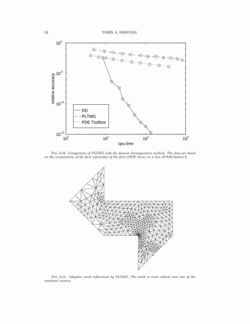
In Figure 3.10 we compare the efficiency of the domain decomposition method tothe computation of the eigenvalues in PLTMG and the PDE Toolbox for Matlab.Figure 3.11 shows the adaptive grid process in PLTMG for the first eigenvalue on thefirst drum. The finest structure occurs near the corner where the eigenfunction is large.At this stage, there are 966 triangles and 402 vertices, and the eigenvalue estimate isabout 2.5659. If one were to try to obtain 12 digits via either of the finite-elementmethods, storage as well as computational time would become a serious obstacle.

One advantage of the domain decomposition method over physical experimentand mode matching is its flexibility in application to other polygons. We have appliedthe domain decomposition method to another pair of isospectral drums, depicted inFigure 3.12. These regions were constructed using the techniques of Buser et al. [5].The fundamental unit of the construction is a (30, 70, 80) triangle, which rendersthe mode matching method impractical. The first 10 eigenvalues of these regions arelisted in Table 3.2 to nine digits. In Figure 3.13 we present the convergence historyanalogous to Figure 3.2. The convergence is again much faster than the minimumrate of ω ≈ 0.48. Selected eigenfunctions for these drums are displayed in Figure 3.14.

4. Conclusions. Elliptic problems on regions with corners, especially reentrantcorners, are recognized as numerically difficult. Indeed, general-purpose packages suchas PLTMG do not use known information about the singularities of solutions near thecorners, and the method of particular solutions uses this information only globally,restricting its usefulness. There is a mode matching method that exploits certainspecial geometries, but this method does not apply to arbitrary polygons.

4In the mode matching method, the degenerate modes 9 and 21 are not computed but are takenexact.

10 TOBIN A. DRISCOLL

FIG. 3.5. First four eigenfunctions of the GWW isospectral drums. Each is normalized to haveunit amplitude. The contours are at levels −0.8,−0.6, . . . , 0.8.

EIGENMODES OF ISOSPECTRAL DRUMS 11

FIG. 3.6. Eigenfunctions 5–8 of the GWW isospectral drums.

12 TOBIN A. DRISCOLL

FIG. 3.7. Eigenfunctions 1, 3, and 6 of the GWW isospectral drums, as measured by Sridharand Kudrolli in their microwave experiments. Reprinted with permission from S. Sridhar and A.Kudrolli.

The domain decomposition method described above exploits the corner infor-mation in an appropriately local and completely general fashion. The method hasexponential convergence as the size of the approximation basis increases. Using thisalgorithm, we have made the first high-precision determinations of the eigenvalues of

EIGENMODES OF ISOSPECTRAL DRUMS 13

FIG. 3.8. The ninth mode of the GWW drums. This corresponds to the first mode on a(45, 45, 90) triangle.

SK1SK2FD MM

5 10 15 20 2510-8

10-7

10-6

10-5

10-4

10-3

10-2

mode

rela

tive

disc

repa

ncy

FIG. 3.9. Comparison of our results with other determinations of the spectra. Shown are the twosets obtained by Sridhar and Kudrolli by microwave experiments and the results of finite differencesand mode matching reported by Wu et al.

the GWW drums. We have also demonstrated that the method is flexible enough tobe applied to other instances of polygonal isospectral regions.

We do not claim that the algorithm presented here is the only efficient methodpossible for the polygon eigenvalue problem. For example, we have not exploredthe application of h-p finite-element methods [1] or integral equation techniques [17].We do believe, however, that any competitive method will make explicit use of thesolutions’ behavior at the corners.

14 TOBIN A. DRISCOLL

DD PLTMG PDE Toolbox

100 101 102 10310-15

10-10

10-5

100

cpu time

rela

tive

accu

racy

FIG. 3.10. Comparison of PLTMG with the domain decomposition method. The data are basedon the computation of the first eigenvalue of the first GWW drum on a Sun SPARCstation 2.

FIG. 3.11. Adaptive mesh refinement by PLTMG. The mesh is most refined near one of thereentrant corners.

EIGENMODES OF ISOSPECTRAL DRUMS 15

0 1 2 3 4

0

1

2

3

4

0 1 2 3 4

0

1

2

3

4

FIG. 3.12. Two more isospectral regions and the subdivisions used in the domain decompositionmethod.

TABLE 3.2First 10 eigenvalues of the isospectral drums of Figure 3.12.

5.63126379 18.85377577.18148848 19.850947112.7905748 24.180329113.0935554 27.537947117.0680091 30.0098327

3 4 5 6 7 8 910-16

10-14

10-12

10-10

10-8

10-6

10-4

10-2

100

m

λ(m

) –

λ(m

–1)

/λ(m

)

FIG. 3.13. Convergence of the eigenvalue estimates for the second pair of drums. Solid linesare for the first drum, dashed lines are for the second drum, and the dotted line is a multiple of ωm,where ω ≈ 0.48.

16 TOBIN A. DRISCOLL

FIG. 3.14. Eigenmodes 1, 3, 4, and 6 of the second pair of isospectral drums. Modes have unitamplitude and contours are drawn at −0.8,−0.6, . . . , 0.8.

EIGENMODES OF ISOSPECTRAL DRUMS 17

To see more of the eigenfunctions of the GWW drums and some animations ofvibrations arising from selected combinations of the modes, use a WWW browser toopen the URL http://amath.colorado.edu/appm/faculty/tad.

Acknowledgments. I would like to thank David Webb, Peter Doyle, JeanDescloux, S. Sridhar, and Arshad Kudrolli for their cooperation and pointers to rel-evant literature. I am also grateful to Steve Vavasis and Nick Trefethen for theirvaluable comments and suggestions.

REFERENCES

[1] I. BABUSKA AND M. SURI, The P and H-P versions of the finite element method, basic prin-ciples and properties, SIAM Rev., 36 (1994), pp. 578–632.

[2] H. P. BALTES AND E. R. HILF, Spectra of Finite Systems, Bibliographisches Institut,Mannheim, 1976.

[3] R. BANK, PLTMG Users’ Guide 7.0: A Software Package for Solving Elliptic Partial Differ-ential Equations, SIAM, Philadelphia, PA, 1994.

[4] P. BERARD, Transplantation et isospectralite, Math. Ann., 292 (1992), pp. 547–559.[5] P. BUSER, J. CONWAY, P. DOYLE, AND K. SEMMLER, Some planar isospectral domains, Inter-

nat. Math. Res. Notices, (1994), pp. 391–400.[6] T. F. CHAN AND T. P. MATHEW, Domain decomposition algorithms, Acta Numerica, (1994),

pp. 61–143.[7] S. J. CHAPMAN, Drums that sound the same, Amer. Math. Monthly, 102 (1995), pp. 124–138.[8] B. CIPRA, You can’t hear the shape of a drum, Science, 255 (1992), pp. 1642–1643.[9] J. DESCLOUX AND M. TOLLEY, An accurate algorithm for computing the eigenvalues of a

polygonal membrane, Comput. Methods Appl. Mech. Engrg., 39 (1983), pp. 37–53.[10] L. FOX, P. HENRICI, AND C. MOLER, Approximations and bounds for eigenvalues of elliptic

operators, SIAM J. Numer. Anal., 4 (1967), pp. 89–102.[11] C. GORDON, D. WEBB, AND S. WOLPERT, Isospectral plane domains and surfaces via Rie-

mannian orbifolds, Invent. Math., 110 (1992), pp. 1–22.[12] M. KAC, Can one hear the shape of a drum?, Amer. Math. Monthly, 73 part II (1966), pp. 1–23.[13] A. KUDROLLI, private communication, 1995.[14] J. R. KUTTLER AND V. G. SIGILLITO, Eigenvalues of the Laplacian in two dimensions, SIAM

Rev., 26 (1984), pp. 163–193.[15] I. PETERSON, Beating a fractal drum: How a drum’s shape affects its sound, Sci. News, 146

(1994), pp. 184–185.[16] S. SRIDHAR AND A. KUDROLLI, Experiments on not “hearing the shape” of drums, Phys. Rev.

Lett., 72 (1994), pp. 2175–2178.[17] P. M. SWARZTRAUBER, On the numerical solution of the dirichlet problem on a region of

general shape, SIAM J. Numer. Anal., 9 (1973), pp. 300–306.[18] H. WU, D. W. L. SPRUNG, AND J. MARTORELL, Numerical investigation of isospectral cavities

built from triangles, Phys. Rev. E, 51 (1995), pp. 703–708.