Eick, Tan, Steinbach, Kumar: Association Analysis Part1 Organization “Association Analysis” 1. What is Association Analysis? 2. Association Rules 3. The

Eick, Tan, Steinbach, Kumar: Association Analysis Part1

Organization “Association Analysis”

1. What is Association Analysis?

2. Association Rules

3. The APRIORI Algorithm

4. Interestingness Measures

5. Sequence Mining Part2

6. Coping with Continuous Attributes in Association Analysis Part2

7. Mining for Other Associations (short) Part2


Association Analysis

Goal: Find Interesting Relationships between Sets of Variables (Descriptive Data Mining)

Relationships can be: Rules (IF buy-beer THEN buy-diaper) Sequences (Book1-Book2-Book3) Graphs Sets (e.g. describing items that co-locate or share

statistical properties, such as correlation) …

What associations are interesting is determined by measures of interestingness.


Finding Regional Correlation Sets

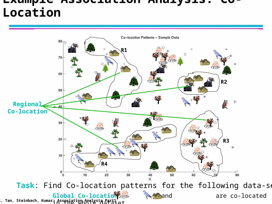
Example Association Analysis: Co-Location

Global Co-location: and are co-located in the whole dataset

Task: Find Co-location patterns for the following data-set.

RegionalCo-location

R1

R2

R3

R4


Association Rule Mining

Given a set of transactions, find rules that will predict the occurrence of an item based on the occurrences of other items in the transaction

Market-Basket transactions

TID Items

1 Bread, Milk

2 Bread, Diaper, Beer, Eggs

3 Milk, Diaper, Beer, Coke

4 Bread, Milk, Diaper, Beer

5 Bread, Milk, Diaper, Coke

Example of Association Rules

{Diaper} {Beer},{Milk, Bread} {Eggs,Coke},{Beer, Bread} {Milk},

Implication means co-occurrence, not causality!


Definition: Frequent Itemset

Itemset– A collection of one or more items

Example: {Milk, Bread, Diaper}

– k-itemset An itemset that contains k items

Support count ()– Frequency of occurrence of an itemset

– E.g. ({Milk, Bread,Diaper}) = 2

Support– Fraction of transactions that contain an

itemset

– E.g. s({Milk, Bread, Diaper}) = 2/5

Frequent Itemset– An itemset whose support is greater

than or equal to a minsup threshold

TID Items

1 Bread, Milk






Definition: Association Rule

Example:Beer}Diaper,Milk{

4.052

|T|)BeerDiaper,,Milk( s

67.032

)Diaper,Milk()BeerDiaper,Milk,(

c

Association Rule– An implication expression of the form

X Y, where X and Y are itemsets

– Example: {Milk, Diaper} {Beer}

Rule Evaluation Metrics– Support (s)

Fraction of transactions that contain both X and Y

– Confidence (c) Measures how often items in Y

appear in transactions thatcontain X

TID Items

1 Bread, Milk






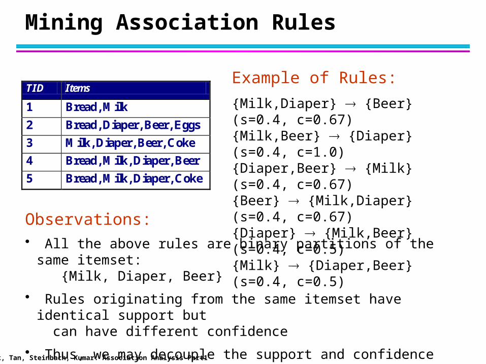
Mining Association Rules

Example of Rules:

{Milk,Diaper} {Beer} (s=0.4, c=0.67){Milk,Beer} {Diaper} (s=0.4, c=1.0){Diaper,Beer} {Milk} (s=0.4, c=0.67){Beer} {Milk,Diaper} (s=0.4, c=0.67) {Diaper} {Milk,Beer} (s=0.4, c=0.5) {Milk} {Diaper,Beer} (s=0.4, c=0.5)

TID Items

1 Bread, Milk





Observations:• All the above rules are binary partitions of the same itemset:

{Milk, Diaper, Beer}

• Rules originating from the same itemset have identical support but can have different confidence

• Thus, we may decouple the support and confidence requirements


Association Rule Mining Task

Given a set of transactions T, the goal of association rule mining is to find all rules having – support ≥ minsup threshold

– confidence ≥ minconf threshold

Brute-force approach:– List all possible association rules

– Compute the support and confidence for each rule

– Prune rules that fail the minsup and minconf thresholds

Computationally prohibitive!


Apriori’s Approach

Two-step approach: 1. Frequent Itemset Generation

– Generate all itemsets whose support minsup

2. Rule Generation– Generate high confidence rules from each frequent itemset,

where each rule is a binary partitioning of a frequent itemset

3. Rule Pruning and Ordering (remove redundant rules; remove/sort rules based on other measures of interesting; e.g. lift)

Frequent itemset generation is still computationally expensive


Frequent Itemset Generation

null

AB AC AD AE BC BD BE CD CE DE

A B C D E

ABC ABD ABE ACD ACE ADE BCD BCE BDE CDE

ABCD ABCE ABDE ACDE BCDE

ABCDE

Given d items, there are 2d possible candidate itemsets


Frequent Itemset Generation

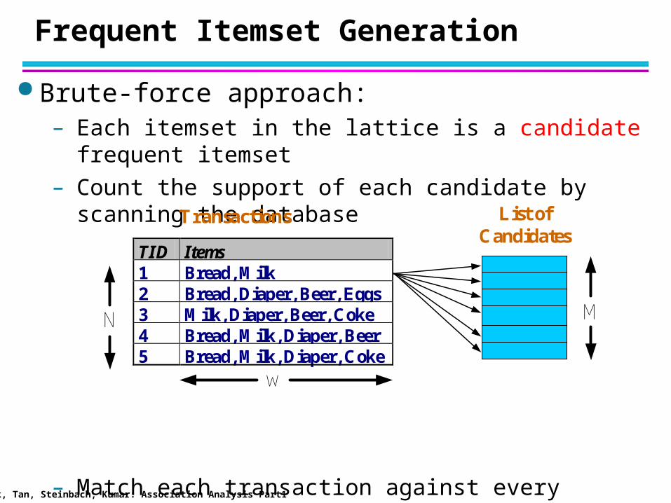
Brute-force approach: – Each itemset in the lattice is a candidate frequent itemset

– Count the support of each candidate by scanning the database

– Match each transaction against every candidate

– Complexity ~ O(NMw) => Expensive since M = 2d !!!

TID Items 1 Bread, Milk 2 Bread, Diaper, Beer, Eggs 3 Milk, Diaper, Beer, Coke 4 Bread, Milk, Diaper, Beer 5 Bread, Milk, Diaper, Coke

N

Transactions List ofCandidates

M

w


Computational Complexity

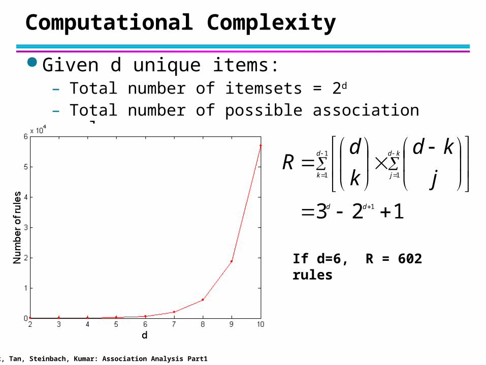
Given d unique items:– Total number of itemsets = 2d

– Total number of possible association rules:

123 1

1

1 1

dd

d

k

kd

j j

kd

k

dR

If d=6, R = 602 rules


Frequent Itemset Generation Strategies

Reduce the number of candidates (M)– Complete search: M=2d

– Use pruning techniques to reduce M

Reduce the number of transactions (N)– Reduce size of N as the size of itemset increases– Used by DHP and vertical-based mining algorithms

Reduce the number of comparisons (NM)– Use efficient data structures to store the candidates or

transactions– No need to match every candidate against every

transaction


Reducing Number of Candidates

Apriori principle:– If an itemset is frequent, then all of its subsets must also be

frequent

Apriori principle holds due to the following property of the support measure:

– Support of an itemset never exceeds the support of its subsets

– This is known as the anti-monotone property of support

)()()(:, YsXsYXYX


Found to be Infrequent

null


A B C D E



ABCDE

Illustrating Apriori Principle

null


A B C D E



ABCDE

Pruned supersets

What do we learn fromThat? If we create k+1-itemsetsfrom k-itemsets we avoidgenerating candidates thatare not frequent due to the Apriori principle.


Illustrating Apriori Principle

Item CountBread 4Coke 2Milk 4Beer 3Diaper 4Eggs 1

Itemset Count{Bread,Milk} 3{Bread,Beer} 2{Bread,Diaper} 3{Milk,Beer} 2{Milk,Diaper} 3{Beer,Diaper} 3

Itemset Count {Bread,Milk,Diaper} 3

Items (1-itemsets)

Pairs (2-itemsets)

(No need to generatecandidates involving Cokeor Eggs)

Triplets (3-itemsets)Minimum Support = 3

If every subset is considered, 6C1 + 6C2 + 6C3 = 41

With support-based pruning,6 + 6 + 1 = 13


Side Discussion: How to store Sets?

Problem: {A, B, C} is the same as {C, B, A}


Apriori Algorithm

Method:

– Let k=1– Generate frequent itemsets of length 1– Repeat until no new frequent itemsets are identified

Generate length (k+1) candidate itemsets from length k frequent itemsets

Prune candidate itemsets containing subsets of length k that are infrequent

Count the support of each candidate by scanning the DB Eliminate candidates that are infrequent, leaving only those that are

frequent– Item sets are represented as sequences based on alphabetic

order; e.g. {a,d,e} is ade. A k+1 item set is constructed from two k-itemsets that agree in their first k-1 items; e.g. abcd and abcg are combined to abcdg.


Mining Association Rules—An Example

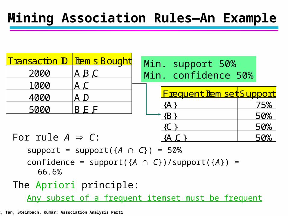
For rule A C:support = support({A C}) = 50%

confidence = support({A C})/support({A}) = 66.6%

The Apriori principle:Any subset of a frequent itemset must be frequent

Transaction ID Items Bought2000 A,B,C1000 A,C4000 A,D5000 B,E,F

Frequent Itemset Support{A} 75%{B} 50%{C} 50%{A,C} 50%

Min. support 50%Min. confidence 50%

The Apriori Algorithm

Join Step: Ck is generated by joining Lk-1with itself

Prune Step: Any (k-1)-itemset that is not frequent cannot be a subset of a frequent k-itemset

Pseudo-code:Ck: Candidate itemset of size k

Lk : frequent itemset of size k

L1 = {frequent items};

for (k = 1; Lk !=; k++) do begin

Ck+1 = candidates generated from Lk;

for each transaction t in database do

increment the count of all candidates in Ck+1 that are contained in t

Lk+1 = candidates in Ck+1 with min_support

end

return k Lk;

The Apriori Algorithm — Example

TID Items100 1 3 4200 2 3 5300 1 2 3 5400 2 5

Database D itemset sup.{1} 2{2} 3{3} 3{4} 1{5} 3

itemset sup.{1} 2{2} 3{3} 3{5} 3

Scan D

C1L1

itemset{1 2}{1 3}{1 5}{2 3}{2 5}{3 5}

itemset sup{1 2} 1{1 3} 2{1 5} 1{2 3} 2{2 5} 3{3 5} 2

itemset sup{1 3} 2{2 3} 2{2 5} 3{3 5} 2

L2

C2 C2

Scan D

C3 L3itemset{2 3 5}

Scan D itemset sup{2 3 5} 2


How to Generate Candidates?

Suppose the items in Lk-1 are listed in an order

Step 1: self-joining Lk-1

insert into Ck

select p.item1, p.item2, …, p.itemk-1, q.itemk-1

from Lk-1 p, Lk-1 q

where p.item1=q.item1, …, p.itemk-2=q.itemk-2, p.itemk-1 < q.itemk-1

Step 2: pruning

forall itemsets c in Ck do

forall (k-1)-subsets s of c do

if (s is not in Lk-1) then delete c from Ck


Example of Generating Candidates

L3={abc, abd, acd, ace, bcd}

Self-joining: L3*L3

– abcd from abc and abd

– acde from acd and ace

Pruning:

– acde is removed because ade is not in L3

C4={abcd}


Factors Affecting Complexity

Choice of minimum support threshold– lowering support threshold results in more frequent itemsets– this may increase number of candidates and max length of

frequent itemsets Dimensionality (number of items) of the data set

– more space is needed to store support count of each item– if number of frequent items also increases, both computation and

I/O costs may also increase Size of database

– since Apriori makes multiple passes, run time of algorithm may increase with number of transactions

Average transaction width– transaction width increases with denser data sets– This may increase max length of frequent itemsets and traversals

of hash tree (number of subsets in a transaction increases with its width)


Rule Generation

Given a frequent itemset L, find all non-empty subsets f L such that f L – f satisfies the minimum confidence requirement– If {A,B,C,D} is a frequent itemset, candidate rules:

ABC D, ABD C, ACD B, BCD A, A BCD, B ACD, C ABD, D ABCAB CD, AC BD, AD BC, BC AD, BD AC, CD AB,

If |L| = k, then there are 2k – 2 candidate association rules (ignoring L and L)


Rule Generation for Apriori Algorithm

ABCD=>{ }

BCD=>A ACD=>B ABD=>C ABC=>D

BC=>ADBD=>ACCD=>AB AD=>BC AC=>BD AB=>CD

D=>ABC C=>ABD B=>ACD A=>BCD

Lattice of rules (for confidence pruning) ABCD=>{ }

BCD=>A ACD=>B ABD=>C ABC=>D

BC=>ADBD=>ACCD=>AB AD=>BC AC=>BD AB=>CD

D=>ABC C=>ABD B=>ACD A=>BCD

Pruned Rules

Low Confidence Rule


Pattern Evaluation

Association rule algorithms tend to produce too many rules – many of them are uninteresting or redundant

– Redundant if {A,B,C} {D} and {A,B} {D} have same support & confidence

Interestingness measures can be used to prune/rank the derived patterns

In the original formulation of association rules, support & confidence are the only measures used


Computing Interestingness Measure

Given a rule X Y, information needed to compute rule interestingness can be obtained from a contingency table

Y Y

X f11 f10 f1+

X f01 f00 fo+

f+1 f+0 |T|

Contingency table for X Yf11: support of X and Yf10: support of X and Yf01: support of X and Yf00: support of X and Y

Used to define various measures

support, confidence, lift, Gini, J-measure, etc.

http://www.eumetcal.org/resources/ukmeteocal/verification/www/english/msg/ver_categ_forec/uos1/uos1_ko1.htm





Statistical Independence

Population of 1000 students– 600 students know how to swim (S)– 700 students know how to bike (B)– 420 students know how to swim and bike (S,B)– In general, between … and … can swim and bike– P(SB) = 420/1000 = 0.42– P(S) P(B) = 0.6 0.7 = 0.42– In general: P(SB)=P(S)*P(B|S)=P(B)*P(S|B)

– P(SB) = P(S) P(B) => Statistical independence– P(SB) > P(S) P(B) => Positively correlated– P(SB) < P(S) P(B) => Negatively correlated– max(0, P(S)+P(B)-1) P(SB) min(P(S),P(B))


Drawback of Confidence

Coffee Coffee

Tea 15 5 20

Tea 75 5 80

90 10 100

Association Rule: Tea Coffee

Confidence= P(Coffee|Tea) = 0.75

but P(Coffee) = 0.9

Þ Although confidence is high, rule is misleading

Þ P(Coffee|Tea) = 0.9375

Problem: Confidence can be large forindependent and negatively correlatedpatterns, if the right hand side pattern has high support.


Statistical-based Measures

Measures that take into account statistical dependence

)](1)[()](1)[(

)()(),(

)()(),(

)()(

),(

)(

)|(

YPYPXPXP

YPXPYXPtcoefficien

YPXPYXPPS

YPXP

YXPInterest

YP

XYPLift

Kind of measure of independence

Correlation for binary Variable

Probability multiplier

Similar to covariance


Drawback of Lift & Interest

Y Y

X 10 0 10

X 0 90 90

10 90 100

Y Y

X 90 0 90

X 0 10 10

90 10 100

10)1.0)(1.0(

1.0 Lift 11.1)9.0)(9.0(

9.0 Lift

Statistical independence:

If P(X,Y)=P(X)P(Y) => Lift = 1

Variables with high priorprobabilities cannot havea high lift--- lift is biased towards variables with low prior probability.

There are lots of measures proposed in the literature

Some measures are good for certain applications, but not for others

What criteria should we use to determine whether a measure is good or bad?

What about Apriori-style support based pruning? How does it affect these measures?


Properties of A Good Measure

Piatetsky-Shapiro: 3 properties a good measure M must satisfy:– M(A,B) = 0 if A and B are statistically independent

– M(A,B) increase monotonically with P(A,B) when P(A) and P(B) remain unchanged

– M(A,B) decreases monotonically with P(A) [or P(B)] when P(A,B) and P(B) [or P(A)] remain unchanged


Comparing Different Measures

Example f11 f10 f01 f00

E1 8123 83 424 1370E2 8330 2 622 1046E3 9481 94 127 298E4 3954 3080 5 2961E5 2886 1363 1320 4431E6 1500 2000 500 6000E7 4000 2000 1000 3000E8 4000 2000 2000 2000E9 1720 7121 5 1154

E10 61 2483 4 7452

10 examples of contingency tables:

Rankings of contingency tables using various measures:


Property under Variable Permutation

B B A p q A r s

A A B p r B q s

Does M(A,B) = M(B,A)?

Symmetric measures:

support, lift, collective strength, cosine, Jaccard, etc

Asymmetric measures:

confidence, conviction, Laplace, J-measure, etc


Different Measures have Different Properties

Sym bol Measure Range P1 P2 P3 O1 O2 O3 O3' O4

Correlation -1 … 0 … 1 Yes Yes Yes Yes No Yes Yes No Lambda 0 … 1 Yes No No Yes No No* Yes No Odds ratio 0 … 1 … Yes* Yes Yes Yes Yes Yes* Yes No

Q Yule's Q -1 … 0 … 1 Yes Yes Yes Yes Yes Yes Yes No

Y Yule's Y -1 … 0 … 1 Yes Yes Yes Yes Yes Yes Yes No Cohen's -1 … 0 … 1 Yes Yes Yes Yes No No Yes No

M Mutual Information 0 … 1 Yes Yes Yes Yes No No* Yes No

J J-Measure 0 … 1 Yes No No No No No No No

G Gini Index 0 … 1 Yes No No No No No* Yes No

s Support 0 … 1 No Yes No Yes No No No No

c Conf idence 0 … 1 No Yes No Yes No No No Yes

L Laplace 0 … 1 No Yes No Yes No No No No

V Conviction 0.5 … 1 … No Yes No Yes** No No Yes No

I Interest 0 … 1 … Yes* Yes Yes Yes No No No No

IS IS (cosine) 0 .. 1 No Yes Yes Yes No No No Yes

PS Piatetsky-Shapiro's -0.25 … 0 … 0.25 Yes Yes Yes Yes No Yes Yes No

F Certainty factor -1 … 0 … 1 Yes Yes Yes No No No Yes No

AV Added value 0.5 … 1 … 1 Yes Yes Yes No No No No No

S Collective strength 0 … 1 … No Yes Yes Yes No Yes* Yes No Jaccard 0 .. 1 No Yes Yes Yes No No No Yes

K Klosgen's Yes Yes Yes No No No No No33

20

3

1321

3

2


Subjective Interestingness Measure

Objective measure: – Rank patterns based on statistics computed from data

– e.g., 21 measures of association (support, confidence, Laplace, Gini, mutual information, Jaccard, etc).

Subjective measure:– Rank patterns according to user’s interpretation A pattern is subjectively interesting if it contradicts the

expectation of a user (Silberschatz & Tuzhilin) A pattern is subjectively interesting if it is actionable

(Silberschatz & Tuzhilin)


Interestingness via Unexpectedness

Need to model expectation of users (domain knowledge)

Need to combine expectation of users with evidence from data (i.e., extracted patterns)

+ Pattern expected to be frequent

- Pattern expected to be infrequent

Pattern found to be frequent

Pattern found to be infrequent

+

-

Expected Patterns-

+ Unexpected Patterns


Association Rule Mining in R

http://www.r-bloggers.com/examples-and-resources-on-association-rule-mining-with-r/

http://www.linkedin.com/groups/Examples-resources-on-association-rule-4066593.S.134055161





Documents

Eick, Tan, Steinbach, Kumar: Association Analysis Part1 Organization “Association Analysis” 1. What is Association Analysis? 2. Association Rules 3. The