EGFD 615 Modern Control - Solution to HW6

Problem 1, part a.: The best way to do this part is to form the controllability test matrix P andthen to take its determinant (which exists because it is 5x5). Letting K1 = K2 = K, I get:

To evaluate the determinant of this 5x5 matrix, it is probably easiest to expand along the firstcolumn, yielding:

Expanding this along the first column gives:

Notice that each of the first two determinants has the bottom two rows eqaul to the negatives ofeach other, and therefore are zero regardless of the value of K. Meanwhile, the third and fourthdeterminants have their first two rows equal, and therefore are also zero regardless of K's value. Thus, det(P) is zero, proving that the system is uncontrollable.

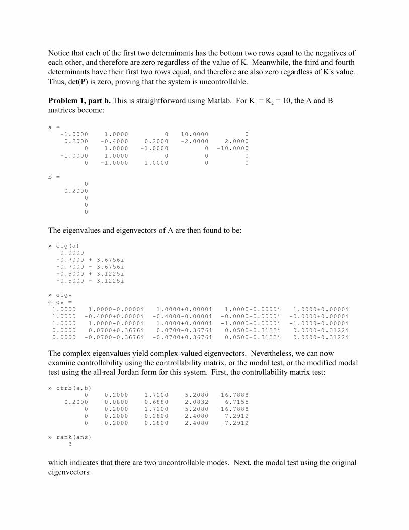
Problem 1, part b. This is straightforward using Matlab. For K1 = K2 = 10, the A and Bmatrices become:

a = -1.0000 1.0000 0 10.0000 0 0.2000 -0.4000 0.2000 -2.0000 2.0000 0 1.0000 -1.0000 0 -10.0000 -1.0000 1.0000 0 0 0 0 -1.0000 1.0000 0 0

b = 0 0.2000 0 0 0

The eigenvalues and eigenvectors of A are then found to be:

» eig(a) 0.0000 -0.7000 + 3.6756i -0.7000 - 3.6756i -0.5000 + 3.1225i -0.5000 - 3.1225i

» eigveigv = 1.0000 1.0000-0.0000i 1.0000+0.0000i 1.0000-0.0000i 1.0000+0.0000i 1.0000 -0.4000+0.0000i -0.4000-0.0000i -0.0000-0.0000i -0.0000+0.0000i 1.0000 1.0000-0.0000i 1.0000+0.0000i -1.0000+0.0000i -1.0000-0.0000i 0.0000 0.0700+0.3676i 0.0700-0.3676i 0.0500+0.3122i 0.0500-0.3122i 0.0000 -0.0700-0.3676i -0.0700+0.3676i 0.0500+0.3122i 0.0500-0.3122i

The complex eigenvalues yield complex-valued eigenvectors. Nevertheless, we can nowexamine controllability using the controllability matrix, or the modal test, or the modified modaltest using the all-real Jordan form for this system. First, the controllability matrix test:

» ctrb(a,b) 0 0.2000 1.7200 -5.2080 -16.7888 0.2000 -0.0800 -0.6880 2.0832 6.7155 0 0.2000 1.7200 -5.2080 -16.7888 0 0.2000 -0.2800 -2.4080 7.2912 0 -0.2000 0.2800 2.4080 -7.2912

» rank(ans) 3

which indicates that there are two uncontrollable modes. Next, the modal test using the originaleigenvectors:

» inv(eigv)*b

0.1429 + 0.0000i

-0.0714 - 0.0136i

-0.0714 + 0.0136i

-0.0000 - 0.0000i

-0.0000 + 0.0000i

The last two values are zero, so the last two modes of the Jordan form (diagonal here) systemdescription, corresponding to the eigenvalues -.5 ± j3.1225 are uncontrollable. [Aside: Sincethese uncontrollable modes are both asymptotically stable, this system is stabilizable. Thismeans that we could, if we wished to, design a state feedback controller for this system thatplaces the three controllable poles wherever we wish. Since one of these poles is at zero, andtherefore is only marginally stable, this is probably a good idea if we want asymptotically stableclosed loop behavior.]

Since the last two modal states are uncontrollable, the modal form of the state space model isalready in Kalman controllability form.

Finally, we try the test on the all-real Jordan form, which we construct by using the real andimaginary parts of the eigenvectors above to build the all-real modal matrix:

m = 1.0000 1.0000 -0.0000 1.0000 -0.0000 1.0000 -0.4000 0.0000 -0.0000 -0.0000 1.0000 1.0000 -0.0000 -1.0000 0.0000 0.0000 0.0700 0.3676 0.0500 0.3122 0.0000 -0.0700 -0.3676 0.0500 0.3122

which we use to convert the original state space description to all-real Jordan form as follows:

» inv(m)*a*m -0.0000 0.0000 -0.0000 -0.0000 -0.0000 0.0000 -0.7000 3.6756 -0.0000 -0.0000 -0.0000 -3.6756 -0.7000 -0.0000 0.0000 0.0000 -0.0000 0.0000 -0.5000 3.1225 -0.0000 0.0000 -0.0000 -3.1225 -0.5000

» inv(m)*b 0.1429 -0.1429 0.0272 -0.0000 0.0000

» c*m 0.0000 0.0000 -0.0000 0.1000 0.6245

Once again, the form we get has a modal form B matrix that indicates the last two modes areuncontrollable, hence this representation is also already in Kalman controllability form. [Notethe form of the transformed C matrix above, which will be used in part d below.]

Problem 1, part c. Now, the A matrix for the system description is:

a = -1.0000 1.0000 0 10.0000 0 0.2000 -0.4000 0.2000 -2.0000 1.0000 0 1.0000 -1.0000 0 -5.0000 -1.0000 1.0000 0 0 0 0 -1.0000 1.0000 0 0

with the B and C matrices as before. Let's check controllability and observability using thecontrollability and observability matrices:

» ctrb(a,b) 0 0.2000 1.7200 -5.0080 -15.5488 0.2000 -0.0800 -0.4880 1.5232 3.4915 0 0.2000 0.7200 -2.6080 -1.9088 0 0.2000 -0.2800 -2.2080 6.5312 0 -0.2000 0.2800 1.2080 -4.1312

» rank(ans) 5

» obsv(a,c) 0 0 0 1 1 -1 0 1 0 0 1 0 -1 -10 -5 9 -5 -4 10 5 -20 12 8 100 15» rank(ans) 4

So we see that now the system is completely controllable but one mode is unobservable. To findthis mode, we find the eigenvalues and eigenvectors of A and use the modal tests forcontrollability and observability:

eig(a) -0.0000 + 0.0000i -0.6428 + 3.4413i -0.6428 - 3.4413i -0.5572 + 2.3240i -0.5572 - 2.3240i

eigv = 1.0000 1.0000+0.0000i 1.0000-0.0000i -0.3047-0.0648i -0.3047+0.0648i 1.0000 -0.2291-0.0208i -0.2291+0.0208i -0.1391+0.0130i -0.1391-0.0130i 1.0000 0.1455+0.1041i 0.1455-0.1041i 1.0000+0.0000i 1.0000-0.0000i -0.0000 0.0586+0.3462i 0.0586-0.3462i 0.0155-0.0750i 0.0155+0.0750i 0.0000 0.0154-0.1117i 0.0154+0.1117i -0.1164-0.4622i -0.1164+0.4622i

» inv(eigv)*b 0.1429 - 0.0000i -0.0894 - 0.0195i -0.0894 + 0.0195i -0.0605 - 0.0075i -0.0605 + 0.0075i

[We already knew the system was completely controllable, but the above result is further proof.]

» c*eigv -0.0000 0.0740+0.2345i 0.0740-0.2345i -0.1009-0.5372i -0.1009+0.5372i

So, we see that the unobservable mode here is the one associated with the eigenvalue at 0. Notethat the system is therefore not detectable because the unobservable mode is only marginallystable. [Physically, recall that the only measurement was the position difference between the“end” masses. Therefore, the “rigid body” motion of the system of masses, i.e. the velocity of thecenter of mass of the entire system, is unobservable. You can see this from the left eigenvector(row of M-1) associated with the unobservable mode, which is a scalar multiple of [1 5 1 0 0]. The velocity of the center of mass of this system is exactly this linear combination of theindividual mass velocities.]

Let’s construct a modal matrix that places the unobservable mode last among the modal statesand produces an all-real version of the Jordan form representation:

m=[real(eigv(:,2)) imag(eigv(:,2)) real(eigv(:,4)) imag(eigv(:,4)) eigv(:,1)]m = 1.0000 0.0000 -0.3047 -0.0648 1.0000 -0.2291 -0.0208 -0.1391 0.0130 1.0000 0.1455 0.1041 1.0000 0.0000 1.0000 0.0586 0.3462 0.0155 -0.0750 -0.0000 0.0154 -0.1117 -0.1164 -0.4622 0.0000

» a_obsv=inv(m)*a*m -0.6428 3.4413 -0.0000 -0.0000 -0.0000 -3.4413 -0.6428 0.0000 -0.0000 0.0000 -0.0000 0.0000 -0.5572 2.3240 -0.0000 0.0000 0.0000 -2.3240 -0.5572 -0.0000 0.0000 -0.0000 -0.0000 -0.0000 0.0000

» b_obsv=inv(m)*b -0.1787 0.0389 -0.1209 0.0151 0.1429

» c_obsv=c*m 0.0740 0.2345 -0.1009 -0.5372 -0.0000

To form the minimal realization, just drop the unobservable mode from the representation:

» a_min=a_obsv(1:4,1:4) -0.6428 3.4413 -0.0000 -0.0000 -3.4413 -0.6428 0.0000 -0.0000 -0.0000 0.0000 -0.5572 2.3240 0.0000 0.0000 -2.3240 -0.5572

» b_min=b_obsv(1:4,:) -0.1787 0.0389 -0.1209 0.0151

» c_min=c_obsv(:,1:4) 0.0740 0.2345 -0.1009 -0.5372

To make sure that the minimal realization is correct, let's check that it produces the same transferfunction as the original system model:

[n,d]=ss2tf(a,b,c,0) % Numerator and denom. of original system T.F. %n = 0 0 0 -0.0000 -1.0000 -0.0000d = 1.0000 2.4000 19.4000 21.0000 70.0000 0.0000

» [n_min,d_min]=ss2tf(a_min,b_min,c_min,0) %Num. & den. of minimalrealization. %n_min = 0 -0.0000 0.0000 0.0000 -1.0000d_min = 1.0000 2.4000 19.4000 21.0000 70.0000

At first glance, it appears that the transfer functions are different because the original has morecoefficients. But note that the last coefficient in both n and d for the original system model iszero. Matlab has failed to recognize a pole-zero cancellation (at s=0) here. If we cancel this poleand zero, the transfer functions are identical.

Problem 1, part d. In part a., we got the transformed C matrix for the modal form of the Kalmancontrollability form. We see from it that the first three modes of the Kalman controllability formare unobservable while the remaining two modes, which are uncontrollable, are observable. Since a minimal realization retains only modes that are both controllable and observable, in thiscase this realization has no dynamics, and the corresponding input/output transfer function is just0 ! [By the way, this does not mean that “there is no system.” Instead, the dynamic system thatexists is such that the input has no effect whatsoever on the output. There could still be nonzerooutputs due to nonzero initial conditions on the observable modes, and there could still be effectsof nonzero inputs on the controllable modes, which do not show up in the outputs.]

Problem 2. The A, B, and C matrices were given on the HW solution for a 6-state realization(there were others!) were:

a = 0 1.0000 0 0 0 0 0 0 1.0000 0 0 0 -20.0000 -39.0000 -14.0000 0 0 0 0 0 0 0 1.0000 0 0 0 0 0 0 1.0000 0 0 0 -20.0000 -39.0000 -14.0000

b = 0 0 0 0 1 0 0 0 0 0 0 1

c = 6 8 2 -4 2 0 1 -2 -1 6 20 0

The eigenvalues and eigenvectors of A are:

eig(a) = -0.6633 -2.8851 -10.4516 -0.6633 -2.8851 -10.4516

eigv = 1.0000 0.1201 0.0092 0 0 0 -0.6633 -0.3466 -0.0957 0 0 0 0.4399 1.0000 1.0000 0 0 0 0 0 0 1.0000 0.1201 0.0092 0 0 0 -0.6633 -0.3466 -0.0957 0 0 0 0.4399 1.0000 1.0000

Note that each eigenvalue is repeated twice. However, it is obvious from the form of theeigenvectors that the two eigenvectors corresponding to each repeated eigenvalue are linearlyindependent, so generalized eigenvectors are not needed here. Forming a modal matrix for achange of basis that groups the two modes corresponding to each eigenvalue together, we get:

» m=[eigv(:,1) eigv(:,4) eigv(:,2) eigv(:,5) eigv(:,3) eigv(:,6)]m = 1.0000 0 0.1201 0 0.0092 0 -0.6633 0 -0.3466 0 -0.0957 0 0.4399 0 1.0000 0 1.0000 0 0 1.0000 0 0.1201 0 0.0092 0 -0.6633 0 -0.3466 0 -0.0957 0 0.4399 0 1.0000 0 1.0000

[Transfo rmed, diag onal A ma trix omitted to s ave space .]

» inv(m)*b 0.0460 0 0 0.0460 -0.4951 0 0 -0.4951 1.4749 0 0 1.4749

» c_modal=c*mc_modal = 1.5738 -5.3265 -0.0520 -1.1737 1.2895 -0.2280 1.8866 -6.3853 -0.1867 -4.2113 -0.7995 0.1413

It is obvious from the modal form of the B matrix that the two rows corresponding to the twomodes associated with each repeated eigenvalue are linearly independent, and hence that thesystem is completely controllable. Recall, however, that the columns of the modal Ccorresponding to modes for a repeated eigenvalue must be not just nonzero, but also linearlyindependent. Among the many checks for linear independence we have, one is to check thedeterminant of the vectors (when the number of vectors is equal to the dimension of the space, asit is here). Checking the determinant of the pair of columns in the modal C matrix correspondingto each repeated eigenvalue, we find:

» det(c_modal(:,1:2)) = -1.8900e-016

» det(c_modal(:,3:4)) = -3.9541e-015

» det(c_modal(:,5:6)) = -2.4157e-015

which are all zero. Hence, this system representation is not observable.

To form a minimal realization, it is tempting at this point to just retain one of the two modesabove corresponding to each repeated eigenvalue and to discard the second mode in each case. Unfortunately, THIS PROCEDURE LEADS TO AN INCORRECT ANSWER because theobservable and unobservable parts of each mode are not correctly separated.

To achieve the proper separation, we need to find, for each pair of modes, a vector (moregenerally, a set of vectors, but here each set has only one element) v such that the linearcombination v1 e1 + v2 e2 = [e1 e2] v of the two eigenvectors e1 and e2 corresponding to a repeatedeigenvalue yields a null vector when multiplied by the original C matrix, i.e. we want v such thatC [e1 e2] v = 0. This linear combination then becomes a (in this case, the one and only, to withina scalar multiple) basis vector for the unobservable subspace corresponding to this particularrepeated eigenvalue. Any linear combination of e1 and e2 that is linearly independent from thisone (or, more generally, from all of these) then yields a nonzero result when multiplied by C, andhence produces a basis vector for the observable subspace.

How do we find these v vectors? Note that we already have C [e1 e2] for each repeatedeigenvalue as the two columns of the modal form C matrix corresponding to each eigenvalue. The v vector(s) for which C [e1 e2] v = 0 can then be found as the right singular vectors of these2x2 partitions of the modal C matrix corresponding to the singular value of zero (and we can usethe right singular vectors corresponding to the nonzero singular values as the coefficients of thelinear combinations of the eigenvectors that yield nonzero results when multiplied by C, thoughthis is not the only way to choose these):

» [u1,s1,v1]=svd(c_modal(:,1:2))[I show u1 here, but the left singular vectors are irrelevant and are omittedhenceforth.]u1 = 0.6406 -0.7679 0.7679 0.6406s1 = 8.6706 0 0 0v1 = 0.2834 -0.9590 -0.9590 -0.2834

» [u2,s2,v2]=svd(c_modal(:,3:4))s2 = 4.3761 0 0 0.0000v2 = 0.0443 -0.9990 0.9990 0.0443

» [u3,s3,v3]=svd(c_modal(:,5:6))s3 = 1.5408 0 0 0.0000v3 = 0.9847 -0.1741 -0.1741 -0.9847

Combining the basis vectors from a previous change of basis in a new way means that we areintroducing a second change of basis, for which there is a new transformation matrix thatexpresses the new basis vectors in terms of the previous basis vectors as its columns. To separatethe observable and unobservable subspaces as required for the Kalman observability form, weput the linear combinations producing nonzero modal C matrix columns in the first threepositions and those producing zero modal C matrix columns in the last three positions. Recallingthat the 2-dimensional right singular vectors in v1 show us how to appropriately combine the firsttwo columns of m (with no components from the remaining four columns of m), those in v2 themiddle two columns of m, and those in v3 the last two columns of m, we construct the newmodal matrix from the previous modal matrix as:

» m_obs=m*[v1(:,1) zeros(2,2) v1(:,2) zeros(2,2); zeros(2,1) v2(:,1) zeros(2,2) v2(:,2) zeros(2,1); zeros(2,2) v3(:,1) zeros(2,2) v3(:,2)]m_obs = 0.2834 0.0053 0.0090 -0.9590 -0.1200 -0.0016 -0.1879 -0.0153 -0.0942 0.6361 0.3463 0.0167 0.1246 0.0443 0.9847 -0.4219 -0.9990 -0.1741 -0.9590 0.1200 -0.0016 -0.2834 0.0053 -0.0090 0.6361 -0.3463 0.0167 0.1879 -0.0153 0.0942 -0.4219 0.9990 -0.1741 -0.1246 0.0443 -0.9847

Now, let's compute our new modal representation of the system dynamics:

» a_obs=inv(m_obs)*a*m_obs -0.6633 0.0000 -0.0000 0.0000 0.0000 -0.0000 -0.0000 -2.8851 -0.0000 -0.0000 0.0000 0.0000 -0.0000 0.0000 -10.4516 0.0000 0.0000 -0.0000 0.0000 0.0000 0.0000 -0.6633 0.0000 -0.0000 0.0000 0.0000 -0.0000 -0.0000 -2.8851 0.0000 -0.0000 0.0000 -0.0000 -0.0000 -0.0000 -10.4516

» b_obs=inv(m_obs)*b 0.0130 -0.0441 -0.0219 -0.4946 1.4524 -0.2568 -0.0441 -0.0130 0.4946 -0.0219 -0.2568 -1.4524

» c_obs=c*m_obs 5.5541 -1.1749 1.3095 0.0000 -0.0000 0.0000 6.6582 -4.2154 -0.8119 0.0000 0.0000 0.0000

The form of this modal C matrix is in the Kalman observability form, which makes it obviousthat now the observable (first three modes of this representation) and unobservable (last threemodes) parts of the system are distinctly separate. Though it is not necessary to do so (because atransformation always preserves controllability and observability), let us check to make sure thatcontrollability has been preserved by checking the linear independence of the rows of the modalB matrix corresponding to each repeated eigenvalue:

» det([b_obs(1,:);b_obs(4,:)]) = -0.0021» det([b_obs(2,:);b_obs(5,:)]) = 0.2452» det([b_obs(3,:);b_obs(6,:)]) = -2.1753

so controllability is preserved. Now the construction of a minimal realization is easy: Just dropthe three unobservable modes:

» a_min=a_obs(1:3,1:3) -0.6633 0.0000 -0.0000 -0.0000 -2.8851 -0.0000 -0.0000 0.0000 -10.4516

» b_min=b_obs(1:3,:) 0.0130 -0.0441 -0.0219 -0.4946 1.4524 -0.2568

» c_min=c_obs(:,1:3) 5.5541 -1.1749 1.3095 6.6582 -4.2154 -0.8119

Finally, let us check to make sure the minimal realization produces the same transfer functionmatrix as the original system model. The original system model yields a 2x2 transfer functionmatrix, and Matlab finds the numerators and denominators as individual columns as:

» [n1,d]=ss2tf(a,b,c,zeros(2,2),1)n1 = 0 2.0000 36.0000 196.0000 436.0000 394.0000 120.0000 0 -1.0000 -16.0000 -66.0000 -84.0000 -1.0000 20.0000d = 1.0e+003 * 0.0010 0.0280 0.2740 1.1320 2.0810 1.5600 0.4000

» [n2,d2]=ss2tf(a,b,c,zeros(2,2),2)n2 = 0 0.0000 2.0000 24.0000 22.0000 -116.0000 -80.0000 0 2.0000 48.0000 364.0000 904.0000 634.0000 120.0000d2 = 1.0e+003 * 0.0010 0.0280 0.2740 1.1320 2.0810 1.5600 0.4000

(Note that the denominator polynomials are identical, as they will always be because they bothhave the 6 system eigenvalues as their roots.) It will be useful to know the poles and zeroes ofthese transfer functions, so let's find the zeroes:

» roots(n1(1,:)) » roots(n1(2,:)) » roots(n2(1,3:7)) » roots(n2(2,:)) -10.4516 -10.4516 -10.4516 -10.4516 -3.0000 -2.8851 2.0000 -9.6904 -2.8851 -2.4142 -2.8851 -2.8851 -1.0000 -0.6633 -0.6633 -0.6633 -0.6633 0.4142 -0.3096

[Note: M ust manually elim inate leading z eros from n 2(1,:) to avo id a huge, inva lid root that M atlab gets.]

and recall that the poles are the eigenvalues of A, which were: -10.4516 (twice), -2.8851 (twice),and -0.6633 (twice). We see that all 4 transfer function matrix elements have zeroes that cancelone of each pair of repeated poles. (The fact that this happens for all 4 numerator elements isimportant because if pole-zero cancellations only happen for some of the numerator elements of atransfer function matrix, this can mean that the transfer function zeroes are not actually thetransmission zeros of the system, and hence that these cancellations merely mean that certainresponse modes do not show up in selected outputs when driven only by selected inputs. Thesemodes may still be controllable and observable, however.) Therefore, we should reduce thetransfer function matrix by eliminating the pole-zero cancellations. To do so, we must factor outthe common factors from each numerator and denominator in the transfer function matrix. Thepolynomial that has the canceled poles as its roots is

» factor=poly([-10.4516 -2.8851 -0.6633])factor = 1.0000 14.0000 39.0000 20.0000

Factoring this out of the denominator polynomial d2 using the Matlab 'deconv' command, we get:

» [q,r]=deconv(d2,factor)q = 1.0000 14.0000 39.0000 20.0000r = 1.0e-010 * 0 0 0 0 0.0500 0.1501 0.0807

where q is the quotient polynomial (which we recognize as having the uncancelled root fromeach pair of roots as its roots) and r is the “remainder” polynomial from the polynomial division,and is clearly negligible. I will omit listing the remainder polynomial hereafter since it is alwayssmall enough to be neglected. Factoring out the common polynomial from the 4 transfer functionnumerators, we get:

» [q11,r11]=deconv(n1(1,:),factor)q11 = 0 2.0000 8.0000 6.0000» [q21,r21]=deconv(n1(2,:),factor)q21 = 0 -1.0000 -2.0000 1.0000» [q12,r12]=deconv(n2(1,:),factor)q12 = 0 0 2.0000 -4.0000» [q22,r22]=deconv(n2(2,:),factor)q22 = 0 2.0000 20.0000 6.0000

Now, let's find the transfer function matrix for the minimal realization and see if it matches:

» [n1_min,d1_min]=ss2tf(a_min,b_min,c_min,zeros(2,2),1)n1_min = 0 2.0000 8.0000 6.0000 0 -1.0000 -2.0000 1.0000d1_min = 1.0000 14.0000 39.0000 20.0000» [n2_min,d2_min]=ss2tf(a_min,b_min,c_min,zeros(2,2),2)n2_min = 0 -0.0000 2.0000 -4.0000 0 2.0000 20.0000 6.0000d2_min = 1.0000 14.0000 39.0000 20.0000

Indeed!

Problem 3. (Problem 10.1 of Bay) The matrix A and its eigenvectors and eigenvalues fromMatlab are:

a = 3 3 0 2 0 87 0 60 6 3 -3 2 0 -126 0 -87» [evec,evl]=eig(a)evec = 0 0.7071 -0.7071 0.0000 0 0 0.0000 -0.5547 1.0000 0.7071 -0.7071 0 0 0 -0.0000 0.8321evl = -3 0 0 0 0 3 0 0 0 0 3 0 0 0 0 -3

So, there are two repeated eigenvalues, a pair at -3 for which two regular eigenvectors exist, anda pair at 3, for which only one regular eigenvector exists. Therefore, we must find thegeneralized eigenvector for the eigenvalue at 3. Using the top-down approach, the index of the

eigenvalue at 3 is clearly 2. Forming the matrix A-3I, we get:

» am3i=a-3*eye(4)am3i = 0 3 0 2 0 84 0 60 6 3 -6 2 0 -126 0 -90» rank(am3i)ans = 3

and the rank calculation verifies that there is only one regular eigenvector. Doing the SVD of(A-3I)2 and of A-3I, we get:

» [u3,s3,v3]=svd(am3i*am3i)u3 = (omitted)s3 = 1.0e+003 * 1.1166 0 0 0 0 0.0509 0 0 0 0 0 0 0 0 0 0v3 = 0 0.7071 -0.7071 0 -0.8137 0 0 -0.5812 0 -0.7071 -0.7071 0 -0.5812 0 0 0.8137[u,s,v]=svd(am3i)u = (omitted)s = 186.1666 0 0 0 0 8.4845 0 0 0 0 0.1162 0 0 0 0 0.0000v = 0.0006 -0.7070 0.0097 -0.7071 0.8137 -0.0072 -0.5812 0.0000 -0.0006 0.7070 -0.0097 -0.7071 0.5812 0.0117 0.8137 -0.0000

For the generalized eigenvector, we need a solution vector g of (A-3I)2 g = 0 that also yields(A-3I) g NOT equal to zero. So, g must be in the nullspace of (A-3I)2, which is spanned by thelast two (orthonormal) columns of v3, but NOT in the nullspace of (A-3I), which is spanned bythe last column of v above. Clearly, we cannot use v3(:,3) as g, but v3(:,4) will work (or it plus amultiple of v3(:,3), but the extra term will contribute nothing to the resulting regulareigenvector). So, let’s use v3(:,4) as g and find from it the corresponding regular eigenvector:

» g=v3(:,4)g = 0 -0.5812 0

0.8137» e1=am3i*ge1 = -0.1162 0.0000 -0.1162 0

For the remaining eigenvectors, we use what Matlab gave above. Hence, a modal matrix, itsinverse, and the resluting Jordan form for A are:

» m=[e1 g evec(:,1) evec(:,4)]m = -0.1162 0 0 0.0000 0.0000 -0.5812 0 -0.5547 -0.1162 0 1.0000 0 0 0.8137 0 0.8321» minv=inv(m)minv = -8.6023 0.0000 0 0.0000 -0.0000 -25.8070 0 -17.2047 -1.0000 0.0000 1.0000 0.0000 0.0000 25.2389 0 18.0278» ja=inv(m)*a*mja = 3.0000 1.0000 0 0.0000 -0.0000 3.0000 0 0.0000 0 -0.0000 -3.0000 -0.0000 -0.0000 0 0 -3.0000

To check the controllability of the modes, construct M-1 B as:

» b1=minv*bb1 = 0.0000 -146.2395 -1.0000 147.8276

The nonzero value (-146.2395) in the second row means that both modes of the 2x2 Jordan blockin ja are controllable. The two remaining nonzero values in b1 are not linearly independent, soONE of the two modes associated with the eigenvalue -3 is NOT controllable. If we add147.8276 times the third row of b1 to the fourth row of b1, we will get 0 in the fourth position, soif we manipulate the rows of the M-1 matrix in the same way, we will get the change of basismatrix required to put the original system representation into Kalman controllability form:

» minv2=minv;minv2(4,:)=minv(4,:)+b1(4)*minv(3,:)minv2 = -8.6023 0.0000 0 0.0000 -0.0000 -25.8070 0 -17.2047 -1.0000 0.0000 1.0000 0.0000 -147.8276 25.2389 147.8276 18.0278» m2=inv(minv2)m2 = -0.1162 -0.0000 -0.0000 0.0000

0.0000 -0.5812 82.0000 -0.5547 -0.1162 0.0000 1.0000 0.0000 0.0000 0.8137 -123.0000 0.8321» akcf=minv2*a*m2akcf = 3.0000 1.0000 -0.0000 0.0000 -0.0000 3.0000 -0.0000 0.0000 0 -0.0000 -3.0000 -0.0000 -0.0000 -0.0000 -0.0000 -3.0000» bkcf=minv2*bbkcf = 0.0000 -146.2395 -1.0000 0.0000

and now we see that akcf and bkcf are in the Kalman controllability form. We can now use thecontrollable part of the representation to do our state feedback calculations (or, if you useMatlab’s ‘place’ command and are careful to include the uncontrollable eigenvalue of -3 amongthe desired poles, you can use the original representation).

The first part of the problem asks us to place the closed loop poles at {-3, -3, -3, -3}. Since -3 isobviously among this set, we can do this. We can use the text’s approach using the multivariablecanonical form of the controllable part of the system, or Matlab’s ‘acker’ command on thecontrollable part, or (sometimes) Matlab’s ‘place’ on either the original representation or thecontrollable part.

Text approach: We form the controllability matrix for the controllable part of the system, and useits last row to form the inverse of the T change of basis matrix as:

» ac=akcf(1:3,1:3);bc=bkcf(1:3);» m1052=ctrb(ac,bc)m1052 = 1.0e+003 * 0.0000 -0.1462 -0.8774 -0.1462 -0.4387 -1.3162 -0.0010 0.0030 -0.0090» minv1053=inv(m1052)minv1053 = 0.0103 -0.0051 -0.2500 0.0000 -0.0011 0.1667 -0.0011 0.0002 -0.0278» m=minv1053(3,:)m = -0.0011 0.0002 -0.0278» t1054=[m;m*ac;m*ac*ac]t1054 = -0.0011 0.0002 -0.0278 -0.0034 -0.0006 0.0833 -0.0103 -0.0051 -0.2500» abar=t1054*ac*inv(t1054)abar = 0.0000 1.0000 -0.0000 0 -0.0000 1.0000 -27.0000 9.0000 3.0000» bbar=t1054*bc

bbar = 0 0.0000 1.0000

So, abar and bbar are in the form for which it is easy to calculate the feedback gains. We willcalculate kbar = [k1 k2 k3] such that abar + bbar*kbar has the companion form of abar but withthe coefficients in the last row such that the closed loop characteristic polynomial is(s+3)(s+3)(s+3) = s3 + 9 s2 + 27 s + 27. This gives k1=0, k2=-36, and k3=-12. Appending a zeroto the gain matrix will account for the neglected, uncontrollable mode. Then, we must unwindthe transformations through T and minv2:

kbar = 0 -36 -12» abar+bbar*kbarans = 0.0000 1.0000 -0.0000 0 -0.0000 1.0000 -27.0000 -27.0000 -9.0000» eig(ans)ans = -2.9999 -3.0001 + 0.0001i -3.0001 - 0.0001i» kc=kbar*t1054kc = 0.2462 0.0821 -0.0000» eig(ac+bc*kc)ans = -3.0001 + 0.0001i -3.0001 - 0.0001i -2.9999 » kkcf=[kc 0];» eig(akcf+bkcf*kkcf)ans = -3.0001 + 0.0001i -3.0001 - 0.0001i -2.9999 -3.0000 » k=kkcf*minv2k = -2.1176 -2.1176 -0.0000 -1.4118» eig(a+b*k)ans = -2.9999 + 0.0002i -2.9999 - 0.0002i -3.0003 -3.0000

So the gain matrix K = [-2.1176 -2.1176 0 -1.4118] does the job.

Here is the result of using ‘acker’:

» kcacker=-acker(ac,bc,[-3 -3 -3])kcacker = 0.2462 0.0821 -0.0000

» kkcfacker=[kcacker 0]kkcfacker = 0.2462 0.0821 -0.0000 0» kacker=kkcfacker*minv2kacker = -2.1176 -2.1176 -0.0000 -1.4118» eig(a+b*kacker)ans = -2.9997 -3.0002 + 0.0003i -3.0002 - 0.0003i -3.0000

Matlab disallows using ‘place’ on the either representation here because it will not place poleswith multiplicity higher than the number of inputs.

The next part of the problem asks us to place the closed loop poles at {-3, -3, -2, -2}. Again, thisis possible because the set include the uncontrollable pole at -3. We can again use theapproaches above. The desired closed loop characteristic polynomial for the controllable part isnow (s+3)(s+2)(s+2) = s3 + 7 s2 + 16 s + 12. For the textbook approach, the gain matrix kbar isnow:

» kbar=[15 -25 -10]kbar = 15 -25 -10» eig(abar+bbar*kbar)ans = -2.0000 -2.0000 -3.0000» kc=kbar*t1054kc = 0.1710 0.0684 -0.0000» eig(ac+bc*kc)ans = -2.0000 -2.0000 -3.0000» kkcf=[kc 0]kkcf = 0.1710 0.0684 -0.0000 0» eig(akcf+bkcf*kkcf)ans = -2.0000 -2.0000 -3.0000 + 0.0000i -3.0000 - 0.0000i» k=kkcf*minv2k = -1.4706 -1.7647 -0.0000 -1.1765» eig(a+b*k)ans = -2.0000 + 0.0000i -2.0000 - 0.0000i -3.0000 -3.0000

and we get the correct pole placement. For ‘acker’, we get:

» kcacker=-acker(ac,bc,[-3 -2 -2])kcacker = 0.1710 0.0684 -0.0000» kkcfacker=[kcacker 0]kkcfacker = 0.1710 0.0684 -0.0000 0» eig(akcf+bkcf*kkcfacker)ans = -2.0000 -2.0000 -3.0000 + 0.0000i -3.0000 - 0.0000i» kacker=kkcfacker*minv2kacker = -1.4706 -1.7647 -0.0000 -1.1765» eig(a+b*kacker)ans = -2.0000 + 0.0000i -2.0000 - 0.0000i -3.0000 -3.0000

We still cannot use ‘place’ here.

The last part asks us toplace the closed loop eigenvalues at {-2, -2, -2, -2}. Since this set doesNOT include the uncontrollable pole at -3, we CANNOT do this placement.