(e.g., deviation variables!)

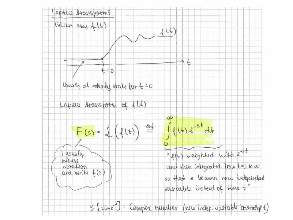
General procedure

1. Nonlinear model

2. Introduce deviation variables and linearize*

3. Laplace of linear model (t ! s)

4. Algebra ! Transfer function, G(s)

5. Block diagram

6. Controller design

*Note: We will only use Laplace for linear systems!

Laplace Transforms

1. Standard notation in dynamics and control for linear systems (shorthand notation)

• Independent variable: Change from t (time) to s (complex variable; inverse time)• Just a mathematical change in variables: Like going from x to y=log(x)

2. Converts differential equations to algebraic operations

3. Advantageous for block diagram analysis.Transfer function, G(s):

Ap

pen

dix

A

G(s)u(s) y(s) = G(s) u(s)

Dynamic system

-st

0

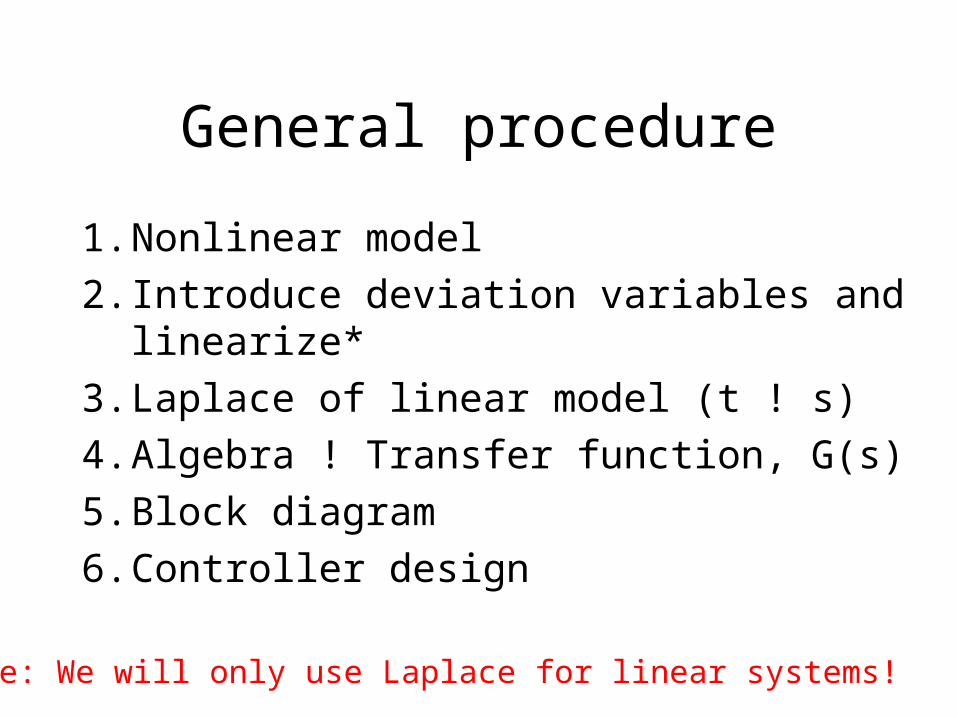
F(s) = L(f (t))= f (t)e dt

Laplace Transform

ExamplesExamples

-st st

00

-bt

-bt -st -(b+s)t ( s)t

00 0

1. f(t)=a (step change)

a a a f(s)= ae dt e 0

s s s

2. f(t)=e

1 1 f(s)= e e dt e dt -e

b+s s+bb

Usually f(t) is in deviation variables so f(t=0) = 0

Definition*:

Ap

pen

dix

A

*Will often misuse notation and write f(s) instead of F(s)

a/s: Laplace of step a

-st

0

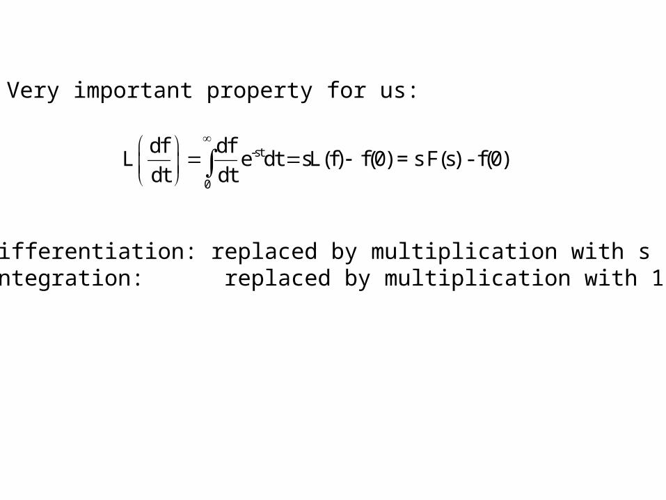
df dfL e dt sL(f) f(0) = s F(s) - f(0)

dt dt

Very important property for us:

Differentiation: replaced by multiplication with sIntegration: replaced by multiplication with 1/s

Table A.1 Laplace Transforms for Various Time-Domain Functionsa

f(t) F(s)

Ap

pen

dix

A

1

0

AREA=1

1

0

Table A.1 Laplace Transforms for Various Time-Domain Functionsa

f(t) F(s)

Ap

pen

dix

A

Table A.1 Laplace Transforms for Various Time-DomainFunctionsa (continued)

f(t) F(s)

Ap

pen

dix

A

Example:Example:

y is deviation variable, system initially at rest (s.s.)

Step 1 Take L.T. (note zero initial conditions)

3 2

3 26 11 6 4

0 0 0 0

d y d y dyy

dt dt dty( )= y ( )= y ( )=

3 2 46 11 6 ( )s Y(s)+ s Y(s)+ sY(s) Y s =

s

Ap

pen

dix

A

Use table

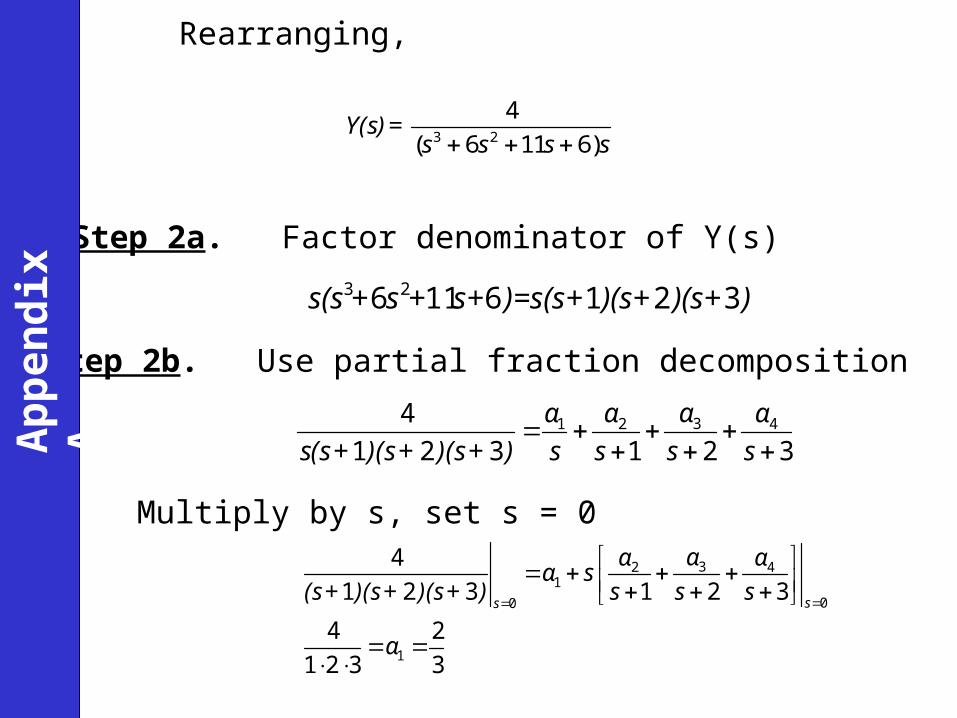
Rearranging,

Step 2a. Factor denominator of Y(s)

Step 2b. Use partial fraction decomposition

Multiply by s, set s = 0

3 2

4

( 6 11 6)Y(s)=

s s s s

))(s+)(s+)=s(s+s++s+s(s 3216116 23

31 2 44

1 2 3 1 2 3

αα α α

s(s+ )(s+ )(s+ ) s s s s

32 41

00

1

4

1 2 3 1 2 3

4 2

1 2 3 3

ss

αα αα s

(s+ )(s+ )(s+ ) s s s

α

Ap

pen

dix

A

For 2, multiply by (s+1), set s=-1 (same procedurefor 3, 4)

2 3 4

22 2

3α , α , α

2 32 22 2

3 32

0 (0) 0.3

t t ty(t)= e e e

t y(t) t y

Step 3. Take inverse of L.T.

You can use this method on any order of ODE, limited only by factoring of denominator polynomial(characteristic equation)

Must use modified procedure for repeated roots, imaginary roots

2 2 2 2 / 3( + )

3 1 2 3Y(s)=

s s s s

(check original ODE)

Ap

pen

dix

A

Use table:

Other properties of Laplace transform:

A. Final value theorem

“steady-state value”

B. Time-shift theorem

y(t)=0 t < θ

sY(s))=y(s 0lim

0

1

1

lim1s

aY(s)

τs sa

y( )= aτs

Y(s)=et-yL s-

Example:

e-µ s : transfer function for time delay µ

Ap

pen

dix

A

C. Initial value theorem

by initial value theorem(multiply Y(s) by s and set s=1)

sY(s)y(t)=st limlim

0

4 2

1

s+For Y(s)=

s(s+ )

0 4y( )=

2y( )= by final value theorem(multiply Y(s) by s and set s=0)

Example

Ap

pen

dix

A

2

0lim ' limt s

y (t)= s Y(s)

D. Initial slope property