EFFICIENT UNCERTAINTY ANALYSIS METHODS FOR

MULTIDISCIPLINARY ROBUST DESIGN

Xiaoping Du* and Wei Chen++++

University of Illinois at Chicago, Chicago, IL 60607, U.S.A.

Copyright © 2001 by Xiaoping Du and Wei Chen. Published by American Institute of aeronautics and Astronautics, Inc., with permission. * Research Assistant, Department of Mechanical Engineering. Member AIAA. + Associate Professor, Department of Mechanical Engineering, weichen1@uic.edu, (312)996-6072. Member AIAA

1

Abstract

Robust design has been gaining wide attention, and its applications have been extended to

making reliable decisions when designing complex engineering systems in a multidisciplinary

design environment. Though the usefulness of robust design is widely acknowledged for

multidisciplinary design systems, its implementation is rare. One of the reasons is due to the

complexity and computational burden associated with the evaluation of performance

variations caused by the randomness (uncertainty) of a system. In this paper, a

multidisciplinary robust design procedure that utilizes efficient methods for uncertainty

analysis is developed. Different from the existing uncertainty analysis techniques, our

proposed techniques bring the features of MDO framework into consideration. The system

uncertainty analysis (SUA) method and the concurrent subsystem uncertainty analysis

(CSSUA) method are developed to estimate the mean and variance of system performance

subject to uncertainties associated with both design parameters and design models. As shown

both analytically and empirically, compared to the conventional Monte Carlo simulation

approach, the proposed techniques used for uncertainty analysis will significantly reduce the

amount of design evaluations at the system level, and therefore improve the efficiency of

robust design in the domain of MDO. A mathematical example and an electronic packaging

problem are used as examples to verify the effectiveness of these approaches.

2

1. Introduction

Robust design has been gaining wide attention and its applications have been extended

from improving the quality of individual components to designing complex engineering

systems. The methods for robust design have progressed from the initial Taguchi�s

�parameter design method� 1 to recent nonlinear programming methods2 - 4 that formulate

robust design problems as nonlinear optimization problems with multiple objectives subject to

feasibility robustness5, 6. Based on its fundamental principle, i.e., improving the quality of a

product by minimizing the effects of variation without eliminating the causes1, robust design

has become one of the powerful tools to assist designers to make reliable decisions under

uncertainty7. In designing complex engineering systems, Multidisciplinary Design

Optimization (MDO) 8-10 has become a systematic approach to optimization of complex,

coupled engineering systems, where �multidisciplinary� refers to the different aspects that

must be included in designing a system that involves multiple interacting disciplines, such as

those found in aircraft, spacecraft, automobiles, and industrial manufacturing applications. It

is generally recognized that there always exist uncertainties in any engineering system due to

variations in design conditions and predictions used in mathematical models7. However, even

though we have seen many applications of MDO, the treatment of uncertainties under

multidisciplinary design has received very limited attention11, 12. There is a great potential to

integrate the robust design concept and the MDO framework for rational decision-making in

designing complex systems.

In recent developments, some preliminary results of robust design for MDO are reported

11 � 14. In these works, response surface models for system level objective and constraints are

created to replace the computationally expensive simulation models. Based on the simplified

3

models, the mean and variance of the system behaviors are evaluated through uncertainty

analysis (propagating the effect of uncertainty) and then utilized to obtain the robust optimal

solutions. When conducting uncertainty analysis, most of these approaches utilize design

evaluations at the system level, namely, the all-in-one approach. The drawback of using the

response surface modeling approach is the cost associated with generating an accurate

response surface model over a large parameter space (for both deterministic and random

variables). Besides, some of the response surface methods tend to �smooth� the behavior.

This results in large errors when the smooth function is used to evaluate local sensitivities in

uncertainty analysis.

In developing efficient methods for uncertainty analysis, many researches have been

focused on design problems with a single discipline or an all-in-one integrated analysis.

Existing methods include Monte Carlo simulation15, first-order second-moment analysis5, 16,

stochastic response surface methods17, polynomial chaos expansion method18, and reliability

analysis based approaches19. Most of these applications are limited to modeling the

uncertainty of input parameters. In recent developments, some preliminary results of

propagating model (structure) uncertainty are reported. Du and Chen7 applied the extreme

condition approach and the statistical approach to propagating the effect of both parameter

and model uncertainties. The extreme condition approach is to derive the range of a system

output in terms of the range of uncertainties by sub-optimizations (minimization and

maximization of the performance). The statistical approach relies heavily on the use of data

sampling to generate probabilistic distributions of system output. Very few works exist on

propagating the effect of uncertainty in the context of multidisciplinary design. Preliminary

results were published recently by Gu et al. 20 on this topic. With their approach, model

4

uncertainty is denoted by a range (bias) of the system output; the �worst case� concept and the

first-order sensitivity analysis are used to evaluate the interval of the end performance of a

multidisciplinary system. Methods that could accommodate generic probabilistic

representations of uncertain parameters and model error estimations have not yet been fully

developed.

Our aim in this paper is to facilitate the integration of the robust design concept with

MDO by developing efficient methods for uncertainty analysis that bring the features of MDO

framework into consideration. To improve the computational efficiency in the context of

highly coupled analyses, two techniques, namely, the system uncertainty analysis (SUA)

method and the concurrent subsystem uncertainty analysis (CSSUA) method, are developed.

The former approach utilizes Taylor expansion as well as local and global sensitivity analysis

(first-order derivatives) to evaluate the mean and variance of a system output, while the later

uses only local sensitivities and a parallel scheme that allows uncertainty analysis

implemented concurrently at the subsystem level. The developed methods will assist

designers to make reliable decisions when there are uncertainties associated with both design

parameters and design models. Both methods will significantly reduce the amount of design

evaluations at the system level, and therefore improve the efficiency of robust design in the

domain of MDO.

Our paper is organized as follows. In Section 2, the need for considering various sources

of uncertainties in simulation-based multidisciplinary system design is addressed along with

the uncertainty representation in a multidisciplinary system. Our proposed methods for

uncertainty analysis and the integration of these methods with MDO are presented in Section

3. In Section 4, Two examples are used to illustrate the effectiveness of our methods. Section

5

5 is the closure which highlights the effectiveness of the proposed methods and provides

discussions on their applicability under different circumstances.

2. Uncertainty Modeling in Simulation-Based Multidisciplinary Design

2.1 Sources of Uncertainties

In simulation-based design, the model-predicted performance and the actual system

performance often deviate at certain levels. Under a multidisciplinary design environment, a

system is composed of multidisciplinary subsystems each using a variety of disciplinary

models with uncertainties associated with performance predications. These subsystems are

often highly coupled where the performance prediction of one discipline may become the

input of another discipline and vice versa 8, 21. A critical issue in simulation-based

multidisciplinary design is that the uncertainties of one discipline may be propagated to

another discipline through the linking variables and the final output from the integrated

multidisciplinary system has an accumulation of the uncertainties from the individual

disciplines. This feature has posed additional challenges in developing efficient uncertainty

analysis techniques for multidisciplinary systems.

Omitting the algorithmic errors related to computer implementations, several general

sources contribute to the uncertainties in simulation predictions:

• Variability of input values x (including both design parameters and design variables),

called �input parameter uncertainty� 7;

• Uncertainty due to limited information in estimating the characteristics of model

parameters p, which are parameter components of a model, e. g. the physical constant

of a model, called �model parameter uncertainty� 22, 23;

6

• Uncertainty in the model structure itself (including uncertainty in the validity of the

assumptions underlying the model), referred to as �model structure uncertainty� 24, 25.

We refer to �input parameter uncertainty� and �model parameter uncertainty� together as

�parameter uncertainty�, and �model structure uncertainty� as �model uncertainty�.

Quantification of model uncertainty is more complicated compared to that of the parameter

uncertainty. It is still an ongoing research issue in both academia and industry 24, 25. We use

the probabilistic notion to suggest that all types of uncertainties studied in this work will be

measured by probability distributions of simulation predictions. One method to consider the

model uncertainty is to introduce a function )(xε of simulation input into the simulation

output function )(xF as

)()( xεxFz += . (1)

Generally, )(xε is a random function even under the condition that x is deterministic.

2.2 Description of Multidisciplinary System under Uncertainties

Fig.1 shows the n-discipline system, where each box represents a simulation program that

belongs to a discipline (or subsystem) for design evaluation. sx are the input variables

considered by more than one subsystem, also called sharing variables. ix )n 1,i( = are the

input variables of subsystem i. Note that sx and ix are mutually exclusive sets of input

variables. Uncertainties may be associated with x s and ix which can be expressed by

probabilistic distributions.

)( jiij ≠y are linking variables, which are those functional outputs calculated in

subsystem i , at the same time, are required as inputs to subsystem j. For simplification of

representation, we denote },,1{ ijnjiji ≠== yy as the set of linking variables generated as

7

outputs from subsystem i and taken as inputs to the other subsystems, and

},,,,{ 111 niii yyyyy �� +−= as the set of linking variables generated as outputs from each of

the subsystem except subsystem i and taken as inputs to subsystem i.

For subsystem i, based on the subsystem simulation model )(⋅yiF and the corresponding

model error )(⋅yiε , the linking variables can be derived as:

),,(),,( iisyi

iisyii yxxεyxxFy += . (2)

Similarly, the general output of subsystem i, )n 1,i( =iz , can be derived as:

),,(),,( iiszi

iiszii yxxεyxxFz += . (3)

The outputs of each subsystem iz , which may include linking variables, are often

associated with the system attributes for the evaluations of constraints and objectives in

optimization. In the situation that an objective (or constraint) is a function of several system

attributes coming from the analyses of different disciplines, a separate subsystem evaluation

can be formed for this purpose.

In propagating the effect of uncertainty, the goal is to quantify the distributions of system

outputs iz for the given parameter uncertainty and the model uncertainty. If we choose to use

the first and second moments (mean value and variance) to describe the distributions, such as

the situation in robust design the problem is stated as:

Given: mean values and variances of input variables xsµ , xiµ , xsσ , and )n 1,i( =xiσ

mean values and variances of model errors yiµ , ziεµ , yiεσ and )n 1,i( =ziεσ Find: mean values and variances of system outputs ziµ and )n 1,i( =ziσ

8

3. Techniques for Uncertainty Analysis in Multidisciplinary Robust Design

Both the system uncertainty analysis (SUA) method and the concurrent subsystem

uncertainty analysis (CSSUA) method are developed to derive the mean and the variance of a

system attribute in a multidisciplinary system. The former approach utilizes Taylor

approximations as well as local and global sensitivity analysis (first-order derivatives), while

the later uses only local sensitivities and a parallel scheme that allows uncertainty analysis

implemented concurrently at the subsystem level. In a distributed design environment, a

parallel scheme is often desired to decouple the multidisciplinary analysis so that individual

groups can work independently from others.

3.1 The SUA method

1) Evaluate mean values

With the SUA method, the mean values of linking variables and system outputs are

approximated at the mean values of inputs as

yiiyxixsyiyi εµµµµFµ += ),,( , (4)

and

ziiyxixsyizi εµµµµFµ += ),,( . (5)

The evaluations of Eqs. (4) and (5) require analyses at the system level.

2) Derive system variance

To obtain the variances of system outputs, firstly, linking variables n) 1,(i =iy are

linearized by the first-order Taylor approximations expanded at the mean values identified

previously in Eq. (4) through system-level evaluations. Multiple linking variables are derived

simultaneously based on a set of linear equations. Secondly, we approximate a system output

by the first-order Taylor expansion with respect to input variables sx , ix and linking

9

variables iy in each subsystem. After substituting iy with the approximation derived earlier,

we have the approximation of a system output as the function of input variables sx , ix only.

Finally, based on the approximated system output, its variance is evaluated. The detailed

procedure is as follows.

From Eq. (2), the linking variables iy are approximated using Taylor�s expansion as

yiii

yis

s

yij

n

ijj j

yii εx

xF

xxF

yyF

y ∆+∆∂∂

+∆∂∂

+∆∂∂

=∆ �≠=1

, (i=1, n) (6)

which can be written in a matrix form

DxCxByA +∆+∆=∆ s , (7)

where

��������

�

�

��������

�

�

∂∂

−∂∂

−

∂∂

−∂∂

−

∂∂

−∂∂

−

=

nynyn

n

yy

n

yy

IyF

yF

yF

IyF

yF

yF

I

A

�

����

�

�

21

22

1

2

1

2

11

,

��������

�

�

��������

�

�

∂∂

∂∂∂∂

=

s

yn

s

y

s

y

xF

xFxF

B�

2

1

,

��������

�

�

��������

�

�

∂∂

∂∂

∂∂

=

n

yn

y

y

xF

xF

xF

C

�

����

�

�

00

00

00

2

2

1

1

,

��������

�

�

��������

�

�

−

−

−

=

ynyn

yy

yy

ε

ε

ε

µε

µε

µε

D�

22

11

xsss µxx −=∆ ,

�������

�

�

�������

�

�

−

−

−

=∆

xnn

x

x

µx

µx

µx

x�

22

11

, and

��������

�

�

��������

�

�

−

−

−

=∆

ynn

y

y

µy

µy

µy

y�

22

11

.

)n 1,i( =iI are the identity matrixes.

Solving a system of equations in Eq. (7) yields

DAxCAxBAy 111 −−− +∆+∆=∆ s . (8)

10

Similarly, system outputs are approximated as

ziii

zis

s

zij

n

ijj j

zii εx

xFx

xFy

yFz ∆+∆

∂∂+∆

∂∂+∆

∂∂=∆ �

≠=1

, (i=1, n), (9)

which can be expressed by the matrix form

HxGxFyEz +∆+∆+=∆ s∆ xGCAExFBAE ∆++∆+= −− ])([])([ 11s HDEA ++ −1 ,(10)

where

��������

�

�

��������

�

�

∂∂

∂∂

∂∂

∂∂

∂∂

∂∂

=

0

0

0

21

2

1

2

1

2

1

�

����

�

�

yF

yF

yF

yF

yF

yF

E

znzn

n

zz

n

zz

,

��������

�

�

��������

�

�

∂∂

∂∂∂∂

=

s

zn

s

z

s

z

xF

xFxF

F�

2

1

,

��������

�

�

��������

�

�

∂∂

∂∂

∂∂

=

n

zn

z

z

xF

xF

xF

G

�

����

�

�

00

00

00

2

2

1

1

,

�������

�

�

�������

�

�

−

−

−

=∆

znn

z

z

µz

µz

µz

z�

22

11

, and

�������

�

�

�������

�

�

−

−

−

=

znzn

zz

zz

ε

ε

ε

µε

µε

µε

H�

22

11

.

Since in Eq. (10), sx∆ , x∆ , D and H are mutually independent, the variance of the

system output can be expressed as

εε zyxxsz DKDJDIDD +++= , (11)

where

�����

�

�

�����

�

�

=

2

22

21

zn

z

z

z

σ

σσ

D�

,

�����

�

�

�����

�

�

=

2

22

21

yn

y

y

y

σ

σσ

D�

, 2xx σD = ,

�����

�

�

�����

�

�

=

2

22

21

xn

x

x

xs

σ

σσ

D�

,

�����

�

�

�����

�

�

=

2

22

21

ny

y

y

y

ε

ε

ε

ε

σ

σσ

D�

,

�����

�

�

�����

�

�

=

2

22

21

nz

z

z

z

ε

ε

ε

ε

σ

σσ

D�

,

}{ iji=I , 21 })({ ijiji FBAE += − , }{ ijj=J , 21 })({ ijijj GCAE += − , }{ ijk=K ,

21}{ ijijk −= EA , and all the 2σ are the variance vectors.

11

All Ds in Eq. (11) stand for vectors of variance and JI , , K are matrices of derivatives of

linking variables and system outputs with respect to input variables. From this equation, it is

noted that the total variation of a system output is derived as the sum of the variations

contributed by four individual sources, i.e., the uncertainties of the sharing variables sx , the

variation of subsystem input variables ix , the variation of linking variable iy due to model

uncertainty, and the variation of system output iz due to model uncertainty.

3.2 The CSSUA method

In the SUA method, for the evaluation of the mean value of a system output, one analysis

at the system level is required. To avoid any system level analysis in the case that it is very

expensive, we developed the concurrent subsystem uncertainty analysis (CSSUA) method.

The basic idea of the CSSUA method is to facilitate the parallelization of the variance

evaluation for system outputs that are contributed by different subsystems. This is

accomplished by making use of optimization technique to find the means of system output

where only subsystem analyses are involved. Once the means of the system output are

obtained, we use the same procedure as we developed for the SUA method to evaluate the

variances of system output. The procedure is as follows.

1) Find mean values of linking variable by the suboptimization as shown in Fig. 2.

Here, the compatibility of the system is achieved by an optimizer which sets the target

values of the mean values of linking variables and minimizes the deviations between the

targets and those that are actually generated through the subsystems analyses. The idea can be

generated as the following unconstrained optimization model:

Given: mean values of input variables xsµ and xiµ )n 1,i( =

Find: target mean values of linking variable

12

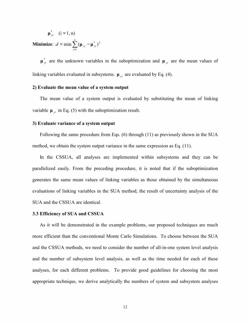
n) 1,i(* =yiµ

Minimize: 2*

1)(min yi

n

iyid µµ −= �

=

*yiµ are the unknown variables in the suboptimization and yiµ are the mean values of

linking variables evaluated in subsystems. yiµ are evaluated by Eq. (4).

2) Evaluate the mean value of a system output

The mean value of a system output is evaluated by substituting the mean of linking

variable yiµ in Eq. (5) with the suboptimization result.

3) Evaluate variance of a system output

Following the same procedure from Eqs. (6) through (11) as previously shown in the SUA

method, we obtain the system output variance in the same expression as Eq. (11).

In the CSSUA, all analyses are implemented within subsystems and they can be

parallelized easily. From the preceding procedure, it is noted that if the suboptimization

generates the same mean values of linking variables as those obtained by the simultaneous

evaluations of linking variables in the SUA method, the result of uncertainty analysis of the

SUA and the CSSUA are identical.

3.3 Efficiency of SUA and CSSUA As it will be demonstrated in the example problems, our proposed techniques are much

more efficient than the conventional Monte Carlo Simulations. To choose between the SUA

and the CSSUA methods, we need to consider the number of all-in-one system level analysis

and the number of subsystem level analysis, as well as the time needed for each of these

analyses, for each different problems. To provide good guidelines for choosing the most

appropriate technique, we derive analytically the numbers of system and subsystem analyses

13

needed for the SUA and the CSSUA methods, respectively, as functions of the number of

input linking variables, the number of subsystem output, the number of sharing variables, the

number of subsystem input variables, and the number of output linking variables.

For each uncertainty analysis, the SUA method needs one system level analysis while the

CSSUA does not require any system level analysis. On the other hand, the CSSUA method

requires more subsystem level analyses (subsystem analyses) than the SUA due to the

suboptimization involved in uncertainty analysis. Assuming that the derivatives needed for

uncertainty analysis (Eqs. 7 and 10) are evaluated numerically, the number of subsystem

analysis for each different method is derived as the following.

1) The number of subsystem analysis for SUA

)]( )(1[)]()([ _1

_ iNiNNiNiNN inputy

n

ixxszoutputySUA +++×+=�

=

, (12)

where )(_ iN outputy - number of output linking variable iy (as the output of subsystem i),

)(iN z - number of system output of subsystem i,

xsN - number of sharing input variables,

)(iN x - number of input variables for subsystem i,

)(_ iN inputy - number of input linking variables iy (as the input for subsystem i).

n � the number of disciplines

The item in the first square brackets is the number of the output of s subsystem and the

item in the second square brackets is the number of the output of a subsystem plus one. The

total number of subsystem analyses is the summation of the number of subsystem analyses of

each subsystem.

2) The number of subsystem analysis for the CSSUA

14

)]( )(1[)]()([ )( _1

_1

__ iNiNNiNiNiNNN inputy

n

ixxszoutputy

n

ioutputycallfunCSSUA +++×++= ��

==

(13)

where Nfun_call is the number of function evaluations for suboptimization.

The first part on the right hand side in Eq. 13 is the number of subsystem analyses for

suboptimization and the second part is the number of subsystem analyses for the variance

evaluations after the suboptimization.

By subtracting Eq. 12 from Eq. 13, we have

SUAcallfunCSSUA NnNN += _ . (14)

The difference of numbers of subsystem analyses of the SUA and the CSSUA becomes

the sum of the number of function evaluations (in suboptimization) multiplies the number of

subsystems, i.e., callfunnN _ . If we can estimate the computational effort for one all-in-one

system analysis as the equivalent number of that for subsystem analyses, then we may prefer

the SUA to CSSUA in the case that the equivalent number of subsystem analyses for the SUA

is less than callfunnN _ , otherwise we would liked to choose the CSSUA.

It should be noted that in the case that parallization (distributed analysis) is considered for

subsystem analysis under the CSSUA, the total amount of time needed (considering the

parallization scheme) will be a better measure than the total number of subsystem analysis

when choosing which method to use.

The proposed methods are developed for MDO implementation considering the features

of a MDO framework. They are in general more efficient than the conventional Monte Carlo

simulation (MCS) approach. To evaluate the means and the standard deviations of system

outputs and linking variables, the MCS will need hundreds of simulations to obtain accurate

estimations, and these simulations need to be conducted at the all-in-one system level. For

15

closed loop systems, this means for each Monte Carlo simulation, multiple subsystem analysis

from each discipline will be needed to reach convergence. The multiplication will often result

in much larger number of subsystem analysis for MCS than for the SUA and CSSUA

methods. In the case that the derivatives needed for uncertainty analysis can be derived

analytically instead of numerically, the advantages of using our proposed methods will be

even more superior than using MCS. In that the case, for each uncertainty analysis, the

computational effort of the proposed methods is similar to the computational effort of only

one simulation of the MCS. In the case that those derivatives need to be evaluated

numerically, the advantages of the SUA and CSSUA methods may diminish when the system

has a very large number of random variables, for example, thousands random variables. In

that case, the MCS approach will be more favorable.

3.4 Formulation of Multidisciplinary Robust Optimization

From the viewpoint of robust design, the goal of a design is to make the system (or

product) inert to the potential variations without eliminating the sources of uncertainty 15. The

same concept is used here to reduce the impact of both parameter and model uncertainties

associated with MDO. The robust optimization objective is achieved by simultaneously

�optimizing the mean performance� and �reducing the performance variation�, subject to the

robustness of constraints5. Let ),( xxa s and ),( xxg s be the objective and constraints of a

system, respectively, the general form of the objective can be expressed as

]),(),,([min xxσxxµ aa ss , (15)

where ),( xxµa s and ),( xxσa s are the mean value and the standard deviation of ),( xxa s ,

respectively and x={x1, x2, …, xn}. Feasibility robustness can be achieved by increasing the

values of constraint functions by the amount of functional variations10 as

16

0≤+ gg σµ k , (16)

where gµ and gσ are the mean values and the standard deviations of ),( xxg s . k is a constant

related to the probability of constraint satisfaction. For example, when ),( xxg s follows the

normal distribution, 1=k corresponds to the probability 8413.0≈ , 2=k the probability

9772.0≈ , etc. The robust design model is summarized as:

Given: Mean and variance of parameter and model uncertainties Find: robust design decisions ( sx and x ) Subject to: system constraints:

0≤+ gg σµ k Objectives: optimize the mean of system attributes ),( xxµa s

minimize the standard deviation of system attributes ),( xxσa s

The mean values aµ and gµ , and the standard deviations aσ and gσ can be obtained by

either the SUA or the CSSUA method. It is noted that if the CSSUA is used, the

suboptimization should be performed under the robust optimization and the whole robust

design will be a double loop procedure. Multiobjective techniques for making tradeoffs

between the mean and variance aspects in robust design have been fully investigated in our

earlier study 26.

The total number of subsystem analyses is approximated equal to the number of function

evaluation of the optimization for robust design times the numbers listed in Eqs. (12) and (13)

for the SUA and the CSSUA respectively. The total number of system analyses for the SUA is

equal to the number of function evaluation of the optimization for robust design.

4. Examples

Two examples are used to illustrate the effectiveness of our proposed uncertainty analysis

techniques. The accuracy of using the SUA and the CSSUA methods for both

17

multidisciplinary design evaluations (analyses) and optimization is examined. To verify the

results, Monte Carlo Simulations (MCS) are also used for both uncertainty analysis and robust

design. A large simulation size, 106, is adopted for each uncertainty analysis and the result

from the MCS is considered as the correct solution for the purpose of confirmation. The

modified feasible direction method is used as the optimizer for both suboptimization for

uncertainty analysis and system optimization for robust design.

4.1 A Mathematical Example

Problem statement

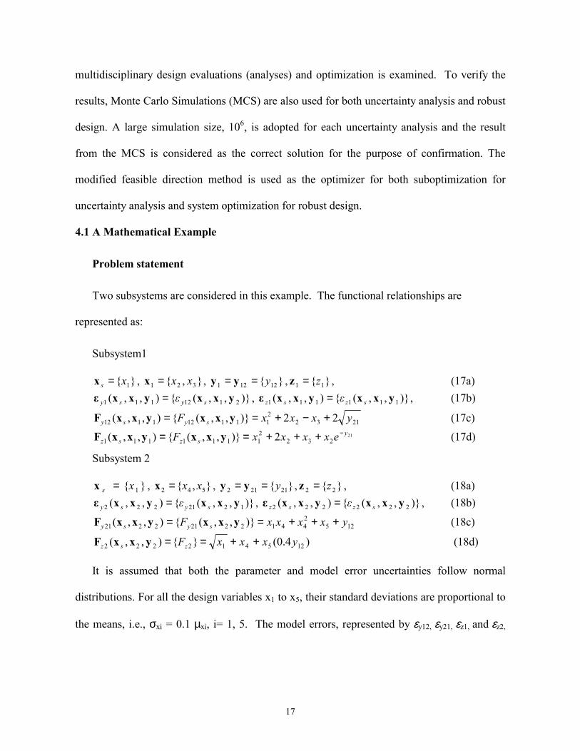
Two subsystems are considered in this example. The functional relationships are

represented as:

Subsystem1

}{ 1xs =x , },{ 321 xx=x , }{ 12121 y== yy , }{ 11 z=z , (17a) )},,({),,( 2112111 yxxyxxε sysy ε= , )},,({),,( 111111 yxxyxxε szsz ε= , (17b)

21322111121112 22)},,({),,( yxxxF sysy +−+== yxxyxxF (17c)

21232

21111111 2)},,({),,( y

szsz exxxxF −+++== yxxyxxF (17d)

Subsystem 2

}{ 1xs =x , },{ 542 xx=x , }{ 21212 y== yy , }{ 22 z=z , (18a) )},,({),,( 1221222 yxxyxxε sysy ε= , )},,({),,( 222222 yxxyxxε szsz ε= , (18b)

125244122212221 )},,({),,( yxxxxF sysy +++== yxxyxxF (18c)

)4.0(}{),,( 125412222 yxxxFzsz ++==yxxF (18d) It is assumed that both the parameter and model error uncertainties follow normal

distributions. For all the design variables x1 to x5, their standard deviations are proportional to

the means, i.e., σxi = 0.1 µxi, i= 1, 5. The model errors, represented by εy12, εy21, εz1, and εz2,

18

have 0 as the means, and the standard deviations being proportional to function values, i.e, 0.1

times the function values.

Accuracy and efficiency for design evaluations

Means and standard deviations of the system outputs z1 and z2 are calculated by the SUA

method and the CSSUA method at three arbitrarily selected design points

=) , , , ,( 54321 xxxxx µµµµµ (1, 1, 1, 1, 1), (2, 2, 2, 2, 2) and (2, 5, 2, 5, 2). The results are compared

in Table 1.

From Table1, it is seen that at all the three points, means of z1 and z2 from the SUA and

the CSSUA methods are almost identical to the results from the MCS. The standard

deviations of z1 and z2 from all the methods are very close with each other. The results from

the SUA and the CSSUA are exactly the same which means the suboptimization in the

CSSUA generates the same values of the linking variables as the SUA does by solving the set

of simultaneous equations. This matches with the discussion in Section 3.2 which states that

the SUA and the CSSUA methods are expected to have the same variance if both methods

generate the same mean values of linking variables. When applying the CSSUA for this

mathematical problem, there are two unknown variables (design variables) in the

suboptimization because the number of linking variables is two.

In this example, the number of subsystem n=2, the number of output

( )()(_ iNiN zoutputy + , i = 1, 2) is 2 for both subsystems 1 and 2. The number of input

( )( )( _ iNiNN inputyxxs ++ , i = 1, 2) is 4 for both subsystems 1 and 2. In terms of the

efficiency of our proposed uncertainty analysis method, for the SUA, the number of system

level analysis is 1 and the number of subsystem analyses is 28. For the CSSUA, the number

of subsystem analyses is 86. The number of system level analysis is 0. These values are

19

consistent with the derived number of function evaluations presented in Section 3.3. For the

MCS, the number of system level analyses is equal to the number of samples used for

simulation, which is 106. If the system level analysis involves close-loop iterative subsystem

analyses, the total number of subsystem analyses will be multiplications of 106.

Accuracy and efficiency for robust design

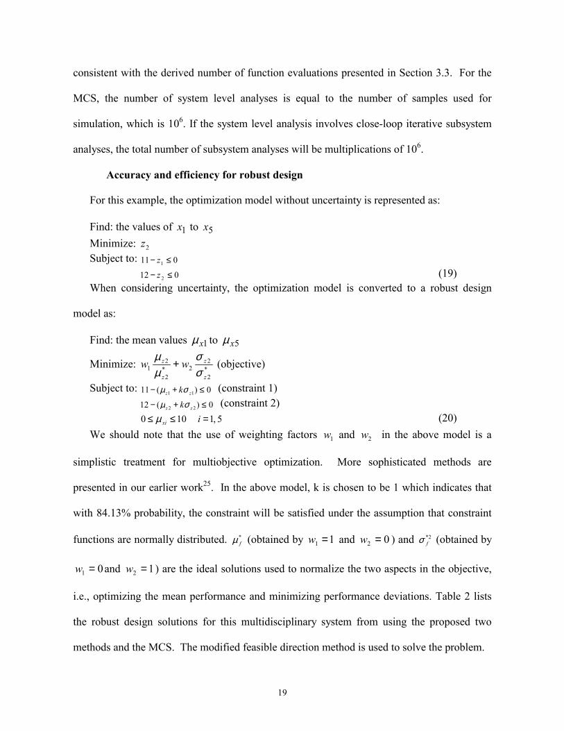
For this example, the optimization model without uncertainty is represented as:

Find: the values of 1x to 5x Minimize: 2z Subject to: 011 1 ≤− z 012 2 ≤− z (19) When considering uncertainty, the optimization model is converted to a robust design

model as:

Find: the mean values 1xµ to 5xµ

Minimize: *2

22*

2

21

z

z

z

z wwσσ

µµ

+ (objective)

Subject to: 0)(11 11 ≤+− zz kσµ (constraint 1) 0)(12 22 ≤+− zz kσµ (constraint 2) 5 ,1 100 =≤≤ ixiµ (20) We should note that the use of weighting factors 1w and 2w in the above model is a

simplistic treatment for multiobjective optimization. More sophisticated methods are

presented in our earlier work25. In the above model, k is chosen to be 1 which indicates that

with 84.13% probability, the constraint will be satisfied under the assumption that constraint

functions are normally distributed. *fµ (obtained by 11 =w and 02 =w ) and 2*

fσ (obtained by

01 =w and 12 =w ) are the ideal solutions used to normalize the two aspects in the objective,

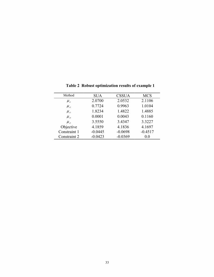
i.e., optimizing the mean performance and minimizing performance deviations. Table 2 lists

the robust design solutions for this multidisciplinary system from using the proposed two

methods and the MCS. The modified feasible direction method is used to solve the problem.

20

The values of the objective and constraints in the last three rows for the SUA and the

CSSUA are the results confirmed by the MCS based on the optimal solutions of 1xµ to 5xµ .

Although the solutions of 1xµ to 5xµ slightly vary from one method to another, we note that

the SUA and the CSSUA methods both generate very close optimal solution to that from the

MCS, in terms of the value of the objective function and the feasibility.

In terms of the efficiency for robust design, for the SUA, the total number of system level

analysis is 31, one for each of the 31 function evaluations of the optimization for robust

design; the total number of subsystem analyses is 868. For the CSSUA, the total number of

subsystem analyses is 2660 (for 35 function evaluations of system level optimization), while

the number of system analysis is 0. When using the MCS, the number of optimization

function evaluation is 46 and the total number of system analyses is equal to 46×106.

4.2 Electronic Packaging Problem

Problem statement

The electronic packaging problem is a benchmark multidisciplinary problem comprising

the coupling between electronic and thermal subsystems. Component resistances (in

electronic subsystem) are affected by operating temperatures in (thermal subsystem), while

the temperatures depend on the resistances. The subsystem relationship is demonstrated in

Fig. 3. A detailed problem statement is provided at http://fmad-

www.larc.nasa.gov/mdob/MDOB.

The system analysis consists of the coupled thermal and electrical analyses. The

component temperatures calculated in the thermal analysis are needed in the electrical

analysis in order to compute the power dissipation of each resistor. Likewise, the power

21

dissipation of each component must be known in order for the thermal analysis to compute the

temperatures.

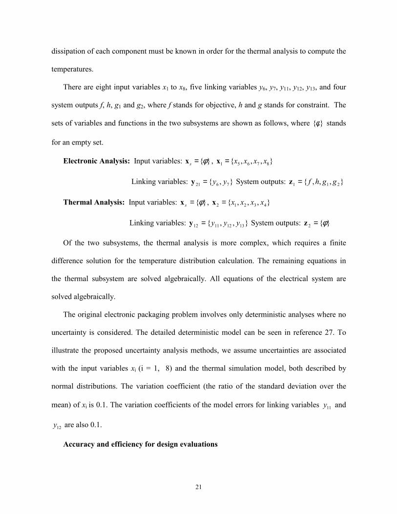
There are eight input variables x1 to x8, five linking variables y6, y7, y11, y12, y13, and four

system outputs f, h, g1 and g2, where f stands for objective, h and g stands for constraint. The

sets of variables and functions in the two subsystems are shown as follows, where }{φ stands

for an empty set.

Electronic Analysis: Input variables: }{φ=sx , },,,{ 87651 xxxx=x

Linking variables: },{ 7621 yy=y System outputs: },,,{ 211 gghf=z

Thermal Analysis: Input variables: }{φ=sx , },,,{ 43212 xxxx=x

Linking variables: },,{ 13121112 yyy=y System outputs: }{2 φ=z

Of the two subsystems, the thermal analysis is more complex, which requires a finite

difference solution for the temperature distribution calculation. The remaining equations in

the thermal subsystem are solved algebraically. All equations of the electrical system are

solved algebraically.

The original electronic packaging problem involves only deterministic analyses where no

uncertainty is considered. The detailed deterministic model can be seen in reference 27. To

illustrate the proposed uncertainty analysis methods, we assume uncertainties are associated

with the input variables xi (i = 1, 8) and the thermal simulation model, both described by

normal distributions. The variation coefficient (the ratio of the standard deviation over the

mean) of xi is 0.1. The variation coefficients of the model errors for linking variables 11y and

12y are also 0.1.

Accuracy and efficiency for design evaluations

22

The accuracy of the SUA and the CSSUA methods for design evaluations are first

compared at two design points with the results from the MCS. The two points are selected

arbitrarily following the normal distribution N(µ, σ):

Point 1: x1-N(0.1, 0.01), x2-N(0.1, 0.01), x3-N(0.1, 0.001), x4-N(0.05, 0.005), x5-N(100,

10), x6-N(0.004, 0.0004), x7-N(100, 10), x8-N(0.004, 0.00041).

Point 2: x1-N(0.08, 0.008), x2-N(0.08, 0.008), x3-N(0.055, 0.0055), x4-N(0.0275, 0.00275),

x5-N(505, 50.5, x6-N(0.0065, 0.00065, x7-N(505, 50.5), x8-N(0.0065, 0.00065).

The modified feasible direction method is used to solve the problem. The results are

shown in Table 3. From Table 3, it is noted that the mean values generated by the SUA and

the CSSUA methods are very close. Those results under h are small enough to be considered

all as zeros. The estimations of standard deviations by using the SUA and the CSSUA are

considered to be satisfactory.

In this example, the number of subsystem n=2, the number of output

( )1()1(_ zoutputy NN + , i = 1, 2) is 6 for subsystem 1 and 3 for subsystem 2. The number of

input ( )( )( _ iNiNN inputyxxs ++ , i = 1, 2) is 7 for subsystem 1 and 6 for subsystem 2. In terms

of efficiency for uncertainty analysis, for the SUA, the number of system analysis is 1 and the

number of subsystem analyses is 82. For the CSSUA, the number of subsystem analyses is

125 (for 43 function evaluations of the suboptimization). The number of system analysis is 0.

For the MCS, the number of system analyses is equal to the number of random samples used

for simulations, which is 106. If the system analysis involves close-loop iterative subsystem

analyses, the total number of subsystem analyses will exceed 106 for each subsystem.

23

Accuracy and efficiency for Robust Optimization

The original deterministic optimization model of the electronic packaging problem is

represented as:

Find: 1x to 8x Minimize: f Subject to: 0≤h 01 ≤g

02 ≤g (21)

When uncertainties are considered, robust design optimization is formulated as

Find: the mean values 1xµ to 8xµ

Minimize: *2*1f

f

f

f wwσσ

µµ

+ (objective)

Subject to: 0≤+ hh kσµ (constraint 1) 011 ≤+ gg kσµ (constraint 2)

022 ≤+ gg kσµ (constraint 3) (22)

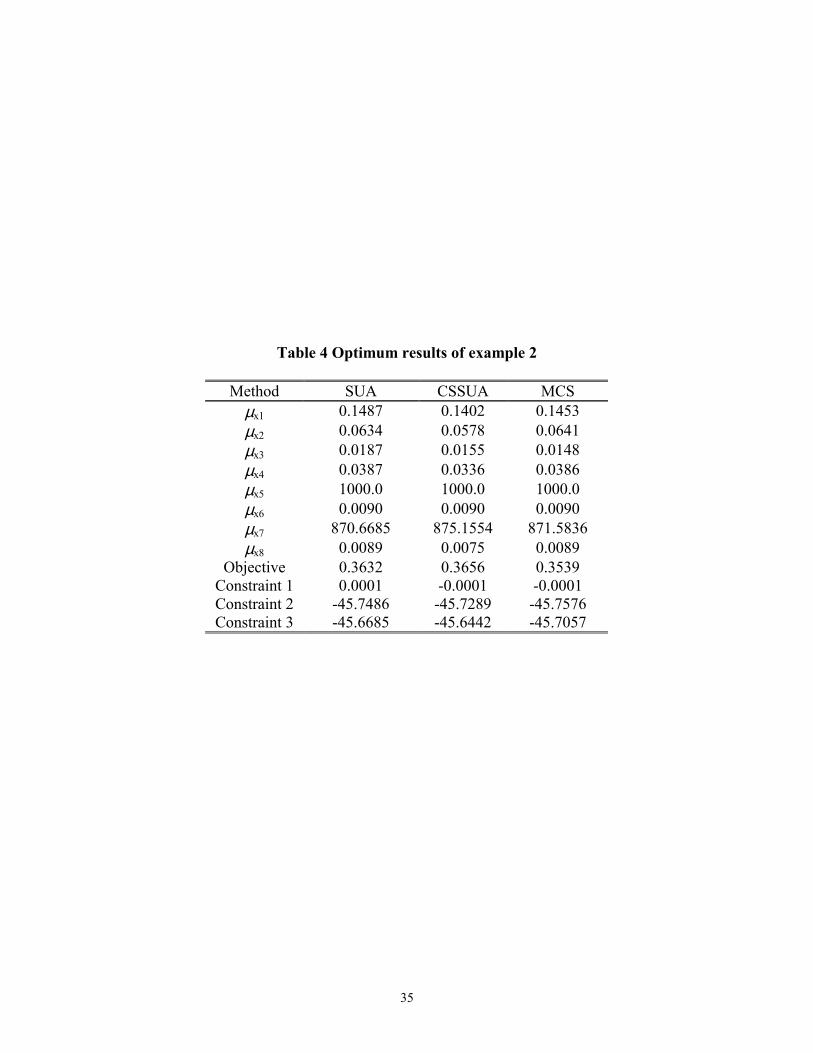
The optimum solutions by different methods are listed in Table 4. Similar to the

mathematical example presented earlier, the values of the objective and constraints for the

SUA and the CSSUA are the results confirmed by the MCS based on the optimal solutions

identified by these two techniques.

We note that the SUA and the CSSUA generate optimum solutions that are close to those

from the MCS, both in the design variable space and the objective space. The most accurate

method is the SUA and the results of the SUA and the CSSUA are slightly different. The

results from all the techniques tested are feasible.

In terms of the efficiency for robust optimization, when using the SUA for uncertainty

analysis, the total number of system analysis is 58, one for each of the 58 function evaluations

in the optimization for robust design; the total number of subsystem analyses is 4756. With

the CSSUA, the total number of subsystem analyses is 7502 (for 62 function evaluations of

24

the system level optimization). With the MCS, the number of system level optimization

function evaluation is 64 and the total number of system analyses is equal to 64×106.

5. Discussions and Closure

Two techniques, namely, the system uncertainty analysis (SUA) method and the

concurrent subsystem uncertainty analysis (CSSUA) method, are developed for improving the

efficiency of uncertainty propagation in simulation-based multidisciplinary design. Both the

parameter uncertainty and model (structure) uncertainty are considered in the proposed

procedures. Since the proposed techniques are developed for evaluating only the mean and

variance of a performance distribution, they are generally applicable for applications where

the first two moments of performance distributions are needed, such as in robust design. The

examples illustrate that both uncertainty analysis methods are applicable in MDO applications

with an acceptable accuracy. Compared to using MCS, both methods can reduce significantly

the all-in-one system level analysis. However, depending on many factors such as the

number of linking variables and the number of disciplines involved, the effectiveness of these

two techniques varies. Considerations should also include the computational needs for

subsystem analyses and the all-in-one integrated system analysis. The SUA method needs one

analysis at the system level for the evaluation of mean values of linking variables and system

output. The accuracy of this evaluation is important because the Taylor approximations used

for variance evaluation are expanded at the mean location. The CSSUA employs a

suboptimization to evaluate mean values of linking variables where only analyses at the

subsystem level are involved. Once mean values of linking variables are obtained, variances

of system output are computed only based on analyses at the subsystem level. Overall the

SUA method needs fewer subsystem level analyses than the CSSUA method, but more

25

system level analyses on the other hand. This feature is demonstrated both analytically in

Section 3.3 and empirically in Section 4 through the example problems. As noted, the

numbers of all-in-one system level analysis and subsystem level analysis are not direct

indications of which method is more efficient. The choice of one method over another highly

depends on the relative magnitude of the time needed for system level analysis and that for

subsystem analysis, and whether parallelization can be accomplished. In general, if the

analysis at the system level is computationally expensive (due to the implicit iteration loops

among subsystems), analyses at the subsystem level are more affordable, and parallelization is

desired, we may use the CSSUA method, and vice versa. In addition to evaluating the total

amount of time need, one should also be aware of the mathematical difficulties related to

optimization convergence of using the CSSUA method. For example, the CSSUA

convergence may be sensitive to the initial values selected for the target means of linking

variables. In a recent paper by Alexandrov and Lewis28, comparative properties of

collaborative optimization and other approaches to MDO are presented. Although their work

is centered on the formulation and computation of multidisciplinary optimization instead of

uncertainty analysis, their discussions on �decomposition and disciplinary autonomy� can also

be used as useful guidelines for us to choose the CSSUA method versus the SUA method.

Interested readers should refer to their paper for further details.

It should be noted that significant computational savings are achieved in this work by

employing Taylor expansions to reduce the amount of couplings among disciplines in

uncertainty analysis. Further, only the first and second moments (mean and variance) are

considered for decision-making under uncertainty and no distributions are needed to

implement the methods. We note that the proceeding assumptions are acceptable for the two

26

multidisciplinary robust design problems illustrated in this paper. However, if high accuracy

is needed (for example in reliability assessment) or the description of the full distribution of a

system output is important, other approaches may be better suited. These approaches are

expected to be generally much more computationally expensive. To further extend the

proposed uncertainty analysis techniques, we plan to investigate computational procedures

that could allow effective sharing between the gradient information obtained for uncertainty

analysis and those needed for system level optimization.

Acknowledgement

The support from the NSF/DMII 9896300 is gratefully acknowledged.

References

1. Phadke, M. S., Quality Engineering using Robust Design, Prentice Hall, Englewood Cliffs, New Jersey, 1989, pp. 6-11.

2. Ramakrishnan, B. and Rao, S.S., �A Robust Optimization Approach Using Taguchi�s Loss Function for Solving Nonlinear Optimization Problems,� Advances in Design Automation, ASME DE-32-1, 1991, pp. 241-248.

3. Sundaresan, S., Ishii, K. and Houser, D.P, �A Robust Optimization Procedure with Variations on Design Variables and Constraints,� Advances in Design Automation, ASME DE-Vol. 69-1, 1993, pp. 379-386.

4. Chen, W., Allen, J.K., Mistree, F. and Tsui, K.-L., �A Procedure for Robust Design: Minimizing Variations Caused by Noise Factors and Control Factors,� ASME Journal of Mechanical Design, Vol. 118, No. 4, 1996, pp.478-485.

5. Du, X. and Chen, W., �Towards a Better Understanding of Modeling Feasibility Robustness in Engineering Design�, ASME Journal of Mechanical Design, Vol. 122, No. 4, 2000, pp. 357-583.

6. Chen W., Sahai, A, Messac, A., and Sundararaj, G.J., �Exploration of the Effectiveness of Physical Programming for Robust Design�, ASME Journal of Mechanical Design, Vol. 22, No. 2, pp. 155-163, 2000.

7. Du, X. and Chen, W., �Methodology for Managing the effect of Uncertainty in Simulation-Based Systems Design�, AIAA Journal, Vol. 38, No. 8, 2000, pp. 1471-1478.

27

8. Balling, R. J. and Sobieski, J., �An Algorithm for Solving the System-Level Problem in Multilevel Optimization�, Structural optimization, Vol. 9, No. 3-4, 1995, pp. 168-177.

9. Renaud, J. E., and Tappeta, R. V., �Multiobjective Collaborative Optimization.� ASME Journal of Mechanical Design, Vol. 119, No. 3, 1997, pp. 403-411.

10. Kroo, I., Altus, S., Braun, R., Gage, P., and Sobieski, I., �Multidisciplinary Optimization Methods for Aircraft Preliminary Design,� AIAA Paper 94-4325, 5th AIAA/USAF/NASA/ISSMO symposium, Panama City Beach, FL, Sep. 1994.

11. Sues, R. H., Oakley, D. R. and Rhodes, G. S., �Multidisciplinary Stochastic Optimization,� Proceedings of the 10th Conference on Engineering Mechanics, Part 2, Vol. 2, Boulder, CO., May 1995, pp. 934-937.

12. Mavris, D.V, Bandte, O. and DeLaurentis, D.A., �Robust Design Simulation: A Probabilistic Approach to Multidisciplinary Design,� Journal of Aircraft, Vol. 36, No. 1, 1999, pp. 298-397.

13. Koch, P.N., Simpson, T.W., Allen, J.K., and Mistree F., �Statistical Approximations for Multidisciplinary Design Optimization: The Problem of Size,� Journal of Aircraft, Vol. 36, No. 1, 1999, pp. 275-286.

14. Batill S., Renaud, J.E., and Gu, X., �Modeling and Simulation in Uncertainty in Multidisciplinary Design Optimization,� AIAA Paper 2000-4803, 8th AIAA/USAF/NASA/ISSMO Symposium on Multidisciplinary Analysis and Optimization, Long Beach, CA, Sept. 2000.

15. Mahadevan, S. and Raghothamachar, P., �Simulation for System Reliability Analysis of Large Structures,� Computers and Structures, Vol. 77, Nov. 6, 2000, pp. 725-734.

16. Hoybye, Jan A., �Model Error Propagation and Data Collection Design, An Application in Water Quality Modeling,� Water, Air and Soil Pollution, Vol. 103, No. 1-4, 1998, pp. 101-119.

17. Isukapalli, S.S, and Georgopoulos, P.G., �Stochastic Response Surface Methods (SRSMs) for Uncertainty Propagation: Application to Environmental and Biological Systems,� Risk Analysis, Vol. 18, No. 3, 1998, pp. 351-363.

18. Wang Cheng, Parametric Uncertainty Analysis for Complex Engineering Systems, Ph.D. Thesis, Jun. 1999, MIT, pp. 53-113.

19. Du, X. and Chen, W., "A Most Probable Point Based Method for Uncertainty Analysis," Journal of Design and Manufacturing Automation, Vol.4, No. 1, 2001, pp. 47-66.

20. Gu, X, Renaud, J. E., and Batill, S. M., �An Investigation of Multidisciplinary Design Subject to Uncertainties,� AIAA Paper 98-4747, 7th AIAA/USAF/NASA/ISSMO Multidisciplinary Analysis & Optimization Symposium, St. Louise, Missouri, Sept. 1998.

28

21. Bloebaum, C. L., Hajela, P. and Sobieszczanski-Sobieski, J., �Non-Hierarchic System Decomposition in Structural Optimization,� Engineering optimization, Vol. 19, No. 3, 1992, pp.171-186.

22. Manners W., �Classification and Analysis of Uncertainty in Structural System,� Proceedings of the 3rd IFIP WG 7.5 Conference on Reliability and Optimization of Structural Systems, Berkeley, California, Mar. 1990, pp.251-260.

23. Ayyub, B.M. and Chao R.U., �Uncertainty Modeling in Civil Engineering with Structural and Reliability Applications,� Uncertainty Modeling and Analysis in Civil Engineering, edited by Ayyub, B.M., 1997, CRC Press, pp. 3-33.

24. Laskey, K. B., �Model Uncertainty: Theory and Practical Implications,� IEEE Transactions on System, Man, and Cybernetics � Part A: System and Human, Vol 26, No. 3, 1996, pp 340-348.

25. Apostolakis, G., �A Commentary on Model Uncertainty, Model Uncertainty: Its Characterization and Quantification,� edited by Mosleh, A, Siu, N, Smidts, C. and Lui, C, NUREG/CP-0138, 1994, U.S. Nuclear Regulatory Commission, pp. 13-22.

26. Chen. W., Wiecek, M., and Zhang, J., �Quality Utility: A Compromise Programming Approach to Robust Design�, ASME Journal of Mechanical Design, Vol. 121, No. 2, 1999, pp.179-187.

27. Du, X. and Chen, W., "An Efficient Approach to Probabilistic Uncertainty Analysis in Simulation-Based Multidisciplinary Design," AIAA Paper: 2000-0423, 38th Aerospace Sciences Meeting and Exhibit, Reno, NV, Jan. 2000.

28. Alexandrov, N.M. and Lewis, R.M., �Comparative Properties of Collaborative Optimization and Other Approaches to MDO�, NASA/CR-1999-209354, ICASE Report No. 99-24, Jul. 1999.

29

Figure 1 Coupled System

xs, x1

z1

xs, x2

z2

xs, xn

zn

y12 y21

y2n yn2

y1n yn1

Subsystem 1 F1(xs, x1, y1) εεεε1(xs, x1, y1)

Fi={Fzi, Fyij , i≠j}, εεεε i={εεεε zi, εεεε yij , i≠j}

Subsystem 2 F2(xs, x2, y2) εεεε2(xs, x2, y2)

Subsystem n Fn (xs, xn, yn) εεεεn (xs, xn, yn)

30

Figure 2 Suboptimization for Uncertainty Analysis in the CSSUA

Suboptimization

SubsystemAnalysis 2

*2yµ

Subsystem Analysis n

*ynµ

*1yµ *

2yµ 3yµ

2*

1)(min yi

n

iyid µµ�

=−=

1yµ 2

yµnyµ

iiy yofmean =µ

Subsystem Analysis 1

*1yµ

31

Figure 3 Information Flow - Electronic Packaging Problem

Electronic Subsystem 1

Thermal Subsystem 2

x5, x6, x7, x8 y6, y7

y11, y12, y13

x1, x2, x3, x4

f, h, g1, g2

32

Table 1 Uncertainty analysis result (mathematical problem)

Method µz1 µz2 σz1 σz2 SUA 4.0000 3.8870 0.5000 0.4764

Point 1 CSSUA 4.0000 3.8870 0.5000 0.4764 MCS 4.0090 3.8780 0.5018 0.4840 SUA 10.0000 8.5130 1.3560 1.1040

Point 2 CSSUA 10.0000 8.5130 1.3560 1.1040 MCS 10.0400 8.5030 1.3580 1.1200 SUA 16.0000 13.1200 2.0590 1.6560

Point 3 SSUA 16.0000 13.1200 2.0590 1.6560 MCS 16.0400 13.1100 2.0680 1.6730

33

Table 2 Robust optimization results of example 1

Method SUA CSSUA MCS 1xµ 2.0700 2.0532 2.1106 2xµ 0.7724 0.9963 1.0104 3xµ 1.8234 1.4822 1.4885 4xµ 0.0001 0.0043 0.1160 5xµ 3.5550 3.4347 3.3227

Objective 4.1859 4.1836 4.1697 Constraint 1 -0.0445 -0.0698 -0.4517 Constraint 2 -0.0423 -0.0369 0.0

34

Table 3 Means and standard deviations of system output at point 1 (example 2)

Method µf σf µh σh µg1 σ g1 µg2 σ g2 SUA -1.847×103 5.363×103 3.901×10-6 1.340×10-2 -44.110 4.046 -44.10 4.390

Point 1 CSSUA -1.847×103 5.363×103 3.901×10-6 1.340×10-2 -44.110 4.046 -44.10 4.390 MCS -1.829×103 5.319×103 1.0×10-11 1.334×10-2 -44.030 4.137 -44.060 4.130 SUA -1.0180×103 1.0490×103 1.713×10-7 2.594×10-3 -48.870 3.586 -48.870 3.649

Point 2 CSSUA -1.0180×103 1.0490×103 1.713×10-7 2.594×10-3 -48.870 3.586 -48.870 3.649 MCS -1.0250×103 1.0690×103 -2.410×10-10 2.663×10-3 -48.850 3.609 -48.880 3.607

35

Table 4 Optimum results of example 2

Method SUA CSSUA MCS µx1 0.1487 0.1402 0.1453 µx2 0.0634 0.0578 0.0641 µx3 0.0187 0.0155 0.0148 µx4 0.0387 0.0336 0.0386 µx5 1000.0 1000.0 1000.0 µx6 0.0090 0.0090 0.0090 µx7 870.6685 875.1554 871.5836 µx8 0.0089 0.0075 0.0089

Objective 0.3632 0.3656 0.3539 Constraint 1 0.0001 -0.0001 -0.0001 Constraint 2 -45.7486 -45.7289 -45.7576 Constraint 3 -45.6685 -45.6442 -45.7057