Efficient subgraph matching using topological node feature constraints

Nicholas Dahma,n, Horst Bunke b, Terry Caelli c, Yongsheng Gao a

a School of Engineering, Griffith University, 170 Kessels Rd, Nathan, Brisbane, QLD, Australiab Institute for Computer Science and Applied Mathematics, University of Bern, Switzerlandc Electrical and Electronic Engineering, University of Melbourne, Australia

a r t i c l e i n f o

Article history:Received 31 August 2013Received in revised form14 May 2014Accepted 28 May 2014Available online 12 June 2014

Keywords:Graph matchingSubgraph isomorphismTopological node features

a b s t r a c t

This paper presents techniques designed to minimise the number of states which are explored duringsubgraph isomorphism detection. A set of advanced topological node features, calculated from n-neighbourhood graphs, is presented and shown to outperform existing features. Further, the pruningeffectiveness of both the new and existing topological node features is significantly improved throughthe introduction of strengthening techniques. In addition to topological node features, these strengthen-ing techniques can also be used to enhance application-specific node labels using a proposed novelextension to existing pruning algorithms. Through the combination of these techniques, the number ofexplored search states can be reduced to near-optimal levels.

& 2014 Elsevier Ltd. All rights reserved.

1. Introduction

In structural pattern recognition, graphs are used to providemeaningful representations of objects and patterns, as well asmore abstract descriptions. The representative power of graphslies in their ability to characterise multiple pieces of information,as well as the relationships between them. These graphs can beused on a variety of applications including network analysis [1],face recognition [2], and image segmentation [3]. However at theheart of graph theory is the problem of graph matching, whichattempts to find a way to map one graph onto another in such away that both the topological structure and the node and edgelabels are matched. For domains where data is noisy, an identicalmatch may not be possible, so an inexact graph matching algo-rithm is used to search for the closest match, minimising somesimilarity function. In this paper, we deal only with exact graphmatching, where a match must be perfect and error-free. Exactgraph matching, due to its nature, is generally used on problemswhere the data is precise and does not contain noise. Examples ofexact graph matching problems include finding chemical simila-rities [4] or substructures [5], protein–protein interaction net-works [6], social network analysis [7], and in the semantic web [8].

Within exact graph matching, there are three graph isomorph-ism problems. These are, in increasing order of complexity, graphisomorphism, subgraph isomorphism, and maximum commonsubgraph isomorphism. While algorithms for all of these problems

have an exponential time complexity in the general case, signifi-cant advances have been made towards making these problemstractable. In this paper we focus on techniques applicable to graphand subgraph isomorphism, with particular emphasis on non-induced subgraph isomorphism. Reviews of algorithms andapproaches for maximum common subgraph isomorphism canbe found in [9–11]. Those looking for a complete survey of graphmatching techniques are directed to [9] for the years up to 2004,and [12] for those since.

One key concept in speeding up graph and subgraph isomorph-ism problems is that of a topological node feature (TNF). A TNF is avalue assigned to a node which encodes information about thelocal graph topology into a simple value. For example, the simplestTNF, namely the node degree, simply counts the number ofadjacent nodes. Topological node features are also known assubgraph isomorphism consistents or, in the case of graph iso-morphism, invariants.

In graph isomorphism, the early Nauty algorithm [13] by McKaywas able to make significant advances beyond existing algorithmsby using TNFs and a strengthening procedure similar to the treeindex method that is presented in this paper. Using these techni-ques, Nauty is able to effectively describe the graph topologysurrounding each node, eliminating mappings to any nodes wherethe topology is not identical. This idea was extended by Sorlin andSolnon to create the IDL algorithm [14]. Some polynomial-timealgorithms have been developed for special cases of graph iso-morphism, such as planar graphs [15] and bounded valence graphs[16]. A recent paper by Fankhauser et al. [17] presents a polynomial-time algorithm for graph isomorphism in the general case. Theirmethod is suboptimal, in that some graph pairs are rejected due tounresolved permutations. However the number of rejected pairs

Contents lists available at ScienceDirect

journal homepage: www.elsevier.com/locate/pr

Pattern Recognition

http://dx.doi.org/10.1016/j.patcog.2014.05.0180031-3203/& 2014 Elsevier Ltd. All rights reserved.

n Corresponding author. Tel.: þ61 7 3735 3753; fax.: þ61 7 3735 5198.E-mail addresses: n.dahm@griffith.edu.au (N. Dahm),

bunke@iam.unibe.ch (H. Bunke), terry.caelli@gmail.com (T. Caelli),yongsheng.gao@griffith.edu.au (Y. Gao).

Pattern Recognition 48 (2015) 317–330

was shown to be only 11 out of 1 620 000 graph pairs (0.00068%)from the MIVIA (previously SIVA) laboratory graph database [18].

Extending such concepts to subgraph isomorphism is challen-ging because, while the subgraph may exist within the full graph,the additional nodes and edges in the full graph create noise forTNFs. This essentially means that instead of searching for TNFswith identical values, algorithms must ensure that TNF valuesfrom subgraph nodes are less than or equal to the correspondingTNF values from the full graph. One of the earliest and mostinfluential subgraph isomorphism algorithms was Ullmann's algo-rithm [19]. Based on a tree search with backtracking, and arefinement procedure to prune the search tree, Ullmann's algo-rithm maintained state of the art performance until being super-seded by the VF2 algorithm. The VF2 algorithm by Cordella et al.[20] has established itself as the benchmark for subgraph iso-morphism algorithms due to its impressive speed, outperformingUllmann's in almost all cases. To achieve such impressive results,VF2 takes subsets of the degree TNF, creating either two values (forundirected graphs), or six values (for directed graphs). The effect ofseparating the degree value into multiple smaller values is that itreduces the chance that TNF noise will prevent an invalid mappingfrom being detected. Despite the impressive reduction of thecomputation complexity provided by VF2, the exponential natureof the subgraph isomorphism problem prevents such algorithmsfrom being practical as the number of nodes increases [21]. Anupdated version of Ullmann's algorithm was recently published[22], which includes a technique called focus search. Focus searchavoids some unnecessary backup and restore operations on thebit-vector domains (representing compatible node mappings)during the search.

A number of recent papers have shown that subgraph iso-morphism can be efficiently solved by utilising constraint program-ming (CP). An early example of this is the nRFþ algorithm byLarrosa and Valiente [23], which is an extension of the non-binaryreally full look ahead (nRF) algorithm. The ILF algorithm byZampelli et al. [24] explored the use of CP with multiple TNFs.The results show that ILF outperforms VF2 on most cases, evenwhen restricted to only the TNF of degree. Another recent CPpaper is the local all different (LAD) algorithm by Solnon [25]. TheLAD constraint ensures that for every compatible node mapping,the nodes adjacent to the subgraph node can be uniquely mappedto nodes adjacent to the full graph node. Each mapping can bevalidated in this way by running the Hopcroft–Karp algorithm[26]. Given x nodes adjacent to the subgraph node and y nodesadjacent to the full graph node, the complexity of validating asingle mapping is Oðxy

ffiffiffiffiffiffiffiffiffiffiffiffixþyÞ

pin the worst case. Despite the high

computational complexity of this step, the pruning power gainedfrom it allows the LAD algorithm to outperform even the ILFalgorithm, on most cases.

This paper presents a number of techniques which can be used tospeed up subgraph isomorphism through the creation, strengthen-ing, and effective use of TNFs. The problem of subgraph isomorphismis formalised in Section 2, as are other definitions and notations usedin this paper. Section 3 introduces the concept of an n-neighbour-hood, and proposes some novel topological features which can becalculated from it. In Section 4, the unified framework is presented,which consists of three TNF strengthening techniques. Thesestrengthening techniques, introduced in Sections 4.1–4.3, can beapplied to TNFs, as well as application-specific node labels. Section4.4 then shows how these concepts can be combined to createstrengthened features that are resistant to noise. Similar to [21], thetechniques discussed in Sections 3 and 4 are designed so that theymay be utilised to enhance any subgraph isomorphism algorithm.

An earlier version of this paper appeared in [27]. In this revisedand extended version, we provide richer descriptions of the pruningtechniques, and employ an improved algorithm for matching nodes

using the tree index, which is considerably faster than its predeces-sor. We also introduce the novel SINEE algorithm in Section 5, whichhas been specifically designed to maximise the effectiveness oftopological node features, as well as the strengthening framework.To evaluate the effectiveness of SINEE, Section 6 provides a morecomprehensive experimental analysis than [27], both analytically andpractically. Finally, in Section 7, a number of conclusions are drawnfrom the experimental results, and future extensions of this work arediscussed.

2. Definitions and notations

The graphs used in this paper are simple (no self-loops, noduplicate edges) unlabelled graphs. However, the adaptation of thetechniques discussed in this paper to non-simple graphs is trivial.

Definition 1 (Graph). A graph is defined as an ordered pairG¼ ðV ; EÞ, where V ¼ fv1;…; vng is a set of vertices and EDV � Vis a set of edges.

The edges of a graph may be either directed E¼ fðvx; vyÞ;…g orundirected E¼ ffvx; vyg;…g. For clarity, undirected graphs are usedto introduce new concepts. The extension of these concepts todirected graphs is also given, for cases where such an extension isnon-trivial.

Subgraph isomorphism detection is performed using a depth-first search. Each state in the search tree represents a permutationof mappings.

Definition 2 (Subgraph Isomorphism State). A subgraph isomorph-ism state S is a quadruple S¼ ðGf ;Gs;M;AÞ, where Gf is the fullgraph, Gs is the subgraph, M is the set of valid mappingsM¼ fðvaAVf-vbAVsÞ;…g, from full graph nodes to subgraphnodes, and A is the set of assigned mappings, such that ADM.

At the root of the search tree is the initial state, where A¼∅.The leaf nodes of the search tree are (possibly invalid) subgraphisomorphisms, where jAj ¼ jVsj.

3. Topological n-neighbourhood features

A topological node feature is defined as any feature which iscalculated solely from the graph topology, as viewed from aparticular node. Existing TNFs utilised for subgraph isomorphisminclude:

� degree: The number of adjacent nodes.� clusterc (clustering coefficient): The number of edges between

adjacent nodes (this does not include edges to the node beingevaluated).

� ncliquesk: The number of cliques of size k that include aparticular node.

� nwalkspk: The number of walks of length k that pass through aparticular node.

Both ncliquesk and nwalkspk are vectors, holding values for eachdifferent k.

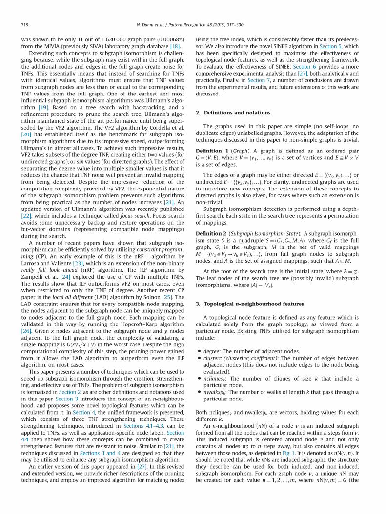
An n-neighbourhood (nN) of a node v is an induced subgraphformed from all the nodes that can be reached within n steps from v.This induced subgraph is centered around node v and not onlycontains all nodes up to n steps away, but also contains all edgesbetween those nodes, as depicted in Fig. 1. It is denoted as nNðv;nÞ. Itshould be noted that while nNs are induced subgraphs, the structurethey describe can be used for both induced, and non-induced,subgraph isomorphism. For each graph node v, a unique nN maybe created for each value n¼ 1;2;…;m, where nNðv;mÞ ¼ G (the

N. Dahm et al. / Pattern Recognition 48 (2015) 317–330318

entire graph can be reached in m steps). In the case of directedgraphs, each nN is replaced by a pair of nNs, one for each direction ofedges leaving the centre node.

Definition 3 (n-Neighbourhood). Given a graph G with node v, ann-neighbourhood nNðv;nÞ is a subgraph G0 ¼ ðV 0; E0Þ, where V 0 isthe set of nodes in G that can be reached within n steps from v,and E0 ¼ ðV 0 � V 0Þ \ E.

There are a number of TNFs that can be calculated from eachnN of a node. Firstly we have the node count, or number of nodesin the nN, denoted by nN-ncount. Likewise we have the edgecount, denoted by nN-ecount. Next we have the number of walksof length k in the nN, denoted nN-nwalksk. Lastly we have thenumber of walks of length k in the nN, that pass through the mainnode, denoted nN-nwalkspk. Each of these TNFs will give adifferent result for each nN of a node, giving n values, or n� pvalues for nN-nwalksk and nN-nwalkspk where k¼ 1;2;…; p. Theprimary benefit of calculating TNFs on nNs is the reduced like-lihood of noise (topological structure not present in the subgraph)from distant nodes being encoded in the feature. For small valuesof n, the features contain less information but also less noise. Onlarger values of n, the amount of information encoded is higher,but so is the likelihood that noise will prevent the feature fromdetecting mismatches.

4. Node label strengthening framework

The node label strengthening framework is a collection of relatedtechniques, designed to propagate, and encode, topological nodefeatures. At the core of the strengthening framework is thesummation, listing, and tree indices, denoted SI, LI, and TI,respectively. In this order, each index utilises a higher-order datastructure than the last, providing greater resolution, while takinglonger to compare. Applied iteratively, this allows a single node tohave distant graph topology encoded into its TNF. In addition topropagating TNFs, the listing and tree indices can also be used topropagate application-specific node labels. When applied to direc-ted graphs, each TNF can be strengthened along either the in-edges, or the out-edges, resulting in two independent values.

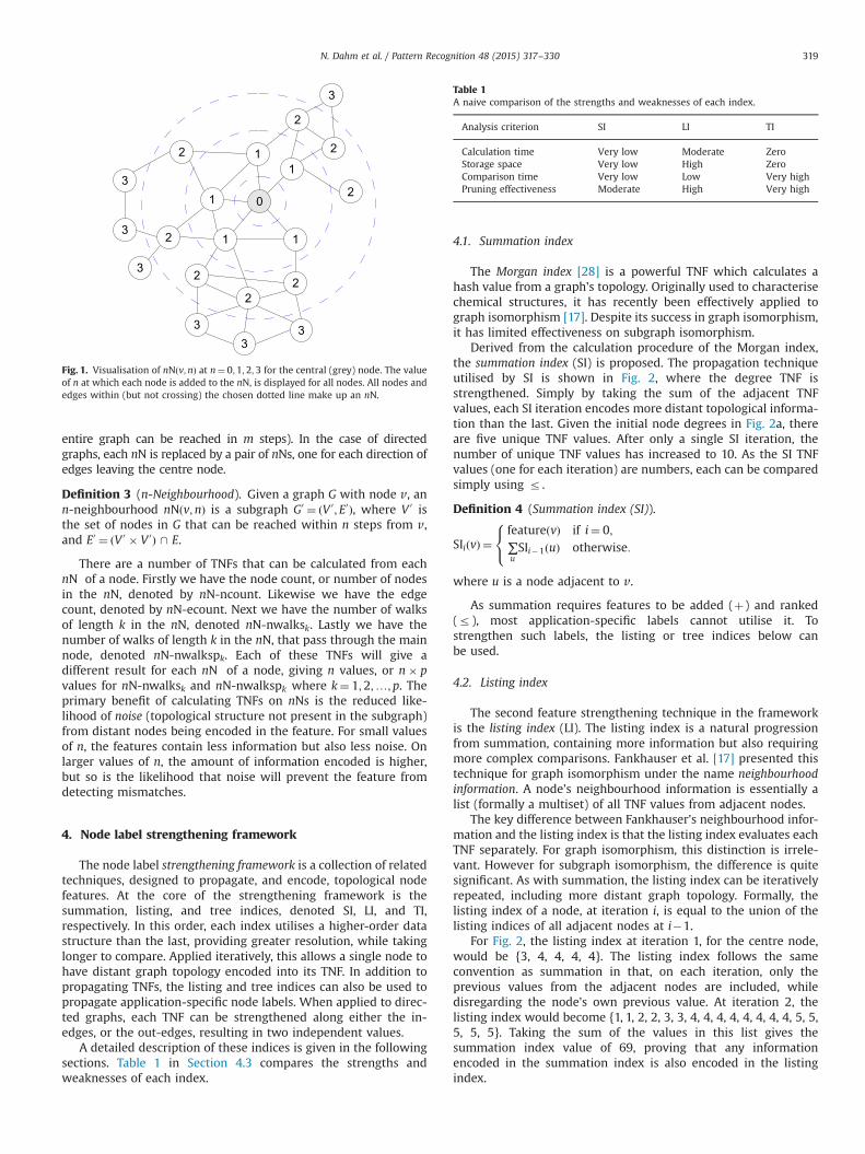
A detailed description of these indices is given in the followingsections. Table 1 in Section 4.3 compares the strengths andweaknesses of each index.

4.1. Summation index

The Morgan index [28] is a powerful TNF which calculates ahash value from a graph's topology. Originally used to characterisechemical structures, it has recently been effectively applied tograph isomorphism [17]. Despite its success in graph isomorphism,it has limited effectiveness on subgraph isomorphism.

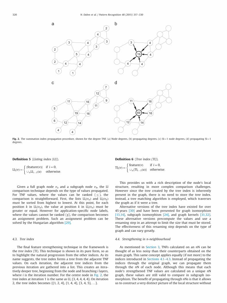
Derived from the calculation procedure of the Morgan index,the summation index (SI) is proposed. The propagation techniqueutilised by SI is shown in Fig. 2, where the degree TNF isstrengthened. Simply by taking the sum of the adjacent TNFvalues, each SI iteration encodes more distant topological informa-tion than the last. Given the initial node degrees in Fig. 2a, thereare five unique TNF values. After only a single SI iteration, thenumber of unique TNF values has increased to 10. As the SI TNFvalues (one for each iteration) are numbers, each can be comparedsimply using r .

Definition 4 (Summation index (SI)).

SIiðvÞ ¼featureðvÞ if i¼ 0;∑uSIi�1ðuÞ otherwise:

8<:

where u is a node adjacent to v.

As summation requires features to be added (þ) and ranked(r), most application-specific labels cannot utilise it. Tostrengthen such labels, the listing or tree indices below canbe used.

4.2. Listing index

The second feature strengthening technique in the frameworkis the listing index (LI). The listing index is a natural progressionfrom summation, containing more information but also requiringmore complex comparisons. Fankhauser et al. [17] presented thistechnique for graph isomorphism under the name neighbourhoodinformation. A node's neighbourhood information is essentially alist (formally a multiset) of all TNF values from adjacent nodes.

The key difference between Fankhauser's neighbourhood infor-mation and the listing index is that the listing index evaluates eachTNF separately. For graph isomorphism, this distinction is irrele-vant. However for subgraph isomorphism, the difference is quitesignificant. As with summation, the listing index can be iterativelyrepeated, including more distant graph topology. Formally, thelisting index of a node, at iteration i, is equal to the union of thelisting indices of all adjacent nodes at i�1.

For Fig. 2, the listing index at iteration 1, for the centre node,would be {3, 4, 4, 4, 4}. The listing index follows the sameconvention as summation in that, on each iteration, only theprevious values from the adjacent nodes are included, whiledisregarding the node's own previous value. At iteration 2, thelisting index would become {1, 1, 2, 2, 3, 3, 4, 4, 4, 4, 4, 4, 4, 4, 5, 5,5, 5, 5}. Taking the sum of the values in this list gives thesummation index value of 69, proving that any informationencoded in the summation index is also encoded in the listingindex.

Fig. 1. Visualisation of nNðv;nÞ at n¼ 0;1;2;3 for the central (grey) node. The valueof n at which each node is added to the nN, is displayed for all nodes. All nodes andedges within (but not crossing) the chosen dotted line make up an nN.

Table 1A naive comparison of the strengths and weaknesses of each index.

Analysis criterion SI LI TI

Calculation time Very low Moderate ZeroStorage space Very low High ZeroComparison time Very low Low Very highPruning effectiveness Moderate High Very high

N. Dahm et al. / Pattern Recognition 48 (2015) 317–330 319

Definition 5 (Listing index (LI)).

LIiðvÞ ¼ffeatureðvÞg if i¼ 0;[uLIi�1ðuÞ otherwise:

(

Given a full graph node va and a subgraph node vb, the LIcomparison technique depends on the type of values propagated.For TNF values, where the values can be ranked (r), thecomparison is straightforward. First, the lists LIiðvaÞ and LIiðvbÞmust be sorted from highest to lowest. At this point, for eachposition k in LIiðvbÞ, the value at position k in LIiðvaÞ must begreater or equal. However for application-specific node labels,where the values cannot be ranked (≰), the comparison becomesan assignment problem. Such an assignment problem can besolved by the Hungarian algorithm [29].

4.3. Tree index

The final feature strengthening technique in the framework isthe tree index (TI). This technique is shown in its pure form, so asto highlight the natural progression from the other indices. As itsname suggests, the tree index forms a tree from the adjacent TNFvalues. On each iteration, the adjacent tree indices from theprevious iteration are gathered into a list. This creates an itera-tively deeper tree, beginning from the node and branching i layers,where i is the iteration number. For the centre node in Fig. 2, thetree index at iteration 1 is the same as LI, {3, 4, 4, 4, 4}. On iteration2, the tree index becomes {{1, 2, 4}, {1, 4, 4}, {3, 4, 5}, …}.

Definition 6 (Tree index (TI)).

TIiðvÞ ¼featureðvÞ if i¼ 0;[ufTIi�1ðuÞg otherwise:

(

This provides us with a rich description of the node's localstructure, resulting in more complex comparison challenges.However since the tree created by the tree index is inherentlypresent in the graph, there is no need to store the tree index.Instead, a tree matching algorithm is employed, which traversesthe graph as if it were a tree.

Alternative versions of the tree index have existed for over45 years [30] and have been presented for graph isomorphism[13,14], subgraph isomorphism [24], and graph kernels [31,32].These alternative versions precompute the values and use arenaming step in an attempt to limit the size that must be stored.The effectiveness of this renaming step depends on the type ofgraph and can vary greatly.

4.4. Strengthening in n-neighbourhood

As mentioned in Section 3, TNFs calculated on an nN can bethought of as less noisy than their counterparts obtained on themain graph. This same concept applies equally (if not more) to theindices introduced in Sections 4.1–4.3. Instead of propagating theindices through the original graph, we can propagate themthrough the nN of each node. Although this means that eachnode's strengthened TNF values are calculated on a unique nNgraph, these values are still valid to compare in subgraph iso-morphism. The benefit of propagating through nNs is that it allowsus to construct a very distinct picture of the local structure without

Fig. 2. The summation index propagation procedure, shown for the degree TNF. (a) Node degrees, (b) propagating degrees, (c) SI¼1 node degrees, (d) propagating SI¼1degrees.

N. Dahm et al. / Pattern Recognition 48 (2015) 317–330320

being distorted by structural information many steps from thenode. The downside to this is that the structure many steps awayis ignored completely, regardless of how useful such informationcould have been. Since nN propagation requires propagatinginformation through each nN separately, the computation requiredis far more than propagation on the main graph. For each nN, thestorage cost is not higher than when propagating on the maingraph. However in general, the nNs and their intermediary nodevalues are kept (to speed up recalculation), so the overall storagecost will be significantly higher.

5. SINEE algorithm

Although these neighbourhood features have been examined indetail, the questions around how to utilise them optimally are stillopen. To this end, we have developed efficient online pruningextensions to the existing iterative node elimination (INE) methods[21]. By eliminating nodes (which caused the elimination ofedges), INE was able to refine TNF values, allowing their pruningpower to be significantly increased. However these eliminationswere all performed prior to any matching, so nodes could only beeliminated when they could not possibly be part of any subgraphisomorphism. With our proposed subgraph isomorphism via nodeand edge elimination (SINEE) algorithm, the elimination of nodesand edges is performed whenever possible throughout the entirematching process to maximise the refinement, and hence thepruning power, of TNFs. As the nN TNFs and strengtheningprocedures described in this paper work on the same principlesas regular TNFs, they can also be refined by the elimination ofnodes and edges.

The advantage to performing node and edge elimination duringthe matching is that the current partial matching restricts theallowable node mappings. For example, suppose we have two fullgraph nodes, va and vb, both of which are only compatible withsubgraph node vc. If the current partial matching has assigned vaas the match for vc, then node vb no longer has any validmappings, so it can be eliminated. Once the current state back-tracks so that va is no longer assigned to vc, then node vb will berestored. Such eliminations are not possible with INE, as they areconditional on the partial matching state.

5.1. Algorithm structure

As with almost all subgraph isomorphism algorithms, SINEE isbased on a depth-first search with pruning. At each search treestate, a new node mapping is added to the partial matching.

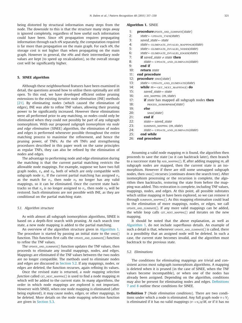
An overview of the algorithm structure given in Algorithm 1.The procedure is started by passing an initial state to the SINEE()function. This function first calls the UPDATE_AND_ELIMINATE() functionto refine the TNF values.

The UPDATE_AND_ELIMINATE() function updates the TNF values, thenproceeds to eliminate any invalid mappings, nodes, and edges.Mappings are eliminated if the TNF values between the two nodesare no longer compatible. The methods used to eliminate nodesand edges are discussed in Section 5.2. If any mappings, nodes, oredges are deleted, the function recurses, again refining its values.

Once the revised state is returned, a node mapping selectionfunction called GET_NEXT_MAPPING() is used to find a node mapping mwhich will be added to the current state. In many algorithms, theorder in which node mappings are explored is not important.However with SINEE, when one node mapping is eliminated (afterbeing explored), it may cause nodes, edges, or other mappings, tobe deleted. More details on the node mapping selection functionare given in Section 5.3.

Algorithm 1. SINEE

1: procedureUPDATE_AND_ELIMINATE(state)2: state’update_tnfsðstateÞ3: saved_state’state4: state’eliminate_invalid_mappingsðstateÞ5: state’eliminate_invalid_nodesðstateÞ6: state’eliminate_invalid_edgesðstateÞ7: if saved_stateastate then8: state’update_and_eliminateðstateÞ9: end if10: return state11: end procedure12: procedure SINEE(state)13: state’update_and_eliminateðstateÞ14: while m’get_next_mappingðÞ do15: saved_state’state16: ADD_MAPPING ðm; stateÞ17: if state has mapped all subgraph nodes then18: PROCESS_ISOMORPHISM(state)19: else20: SINEE(state)21: end if22: state’saved_state23: ELIMINATE_MAPPING ðm; stateÞ24: state’update_and_eliminateðstateÞ25: end while26: end procedure

Assuming a valid node mapping m is found, the algorithm thenproceeds to save the state (so it can backtrack later), then branchto a successor state by ADD_MAPPING(). If, after adding mapping m, allsubgraph nodes are mapped, then the current state is an iso-morphism. However if there are still some unmapped subgraphnodes, then SINEE() recurses (continues down the search tree). Afterisomorphism processing or the recursion is complete, the algo-rithm then backtracks, restoring the state from before the map-ping was added. This restoration is complete, including TNF values,mappings, nodes, and edges. At this point, all possible substateswhich utilise mapping m have been explored, so we can remove itthrough ELIMINATE_MAPPING(). As this mapping elimination could leadto the elimination of more mappings, nodes, or edges, we callUPDATE_AND_ELIMINATE(). If any more valid mappings can be added,the while loop calls GET_NEXT_MAPPING() and iterates on the newmapping.

It should be noted that the above explanation, as well asAlgorithm 1, do not include superfluous details. An example ofsuch a detail is that, whenever UPDATE_AND_ELIMINATE() is called, thereis a possibility that an assigned node will be deleted. In such acase, the current state becomes invalid, and the algorithm mustbacktrack to the previous state.

5.2. Eliminations

The conditions for eliminating mappings are trivial and con-sistent across most subgraph isomorphism algorithms. A mappingis deleted when it is pruned (in the case of SINEE, when the TNFvalues become incompatible), or when one of the nodes hasalready been assigned. Depending on the algorithm, conditionsmay also be present for eliminating nodes and edges. Definitions7 and 8 outline these conditions for SINEE.

Definition 7 (Node elimination conditions). There are two condi-tions under which a node is eliminated. Any full graph node vAVf

is eliminated if it has no valid mappings ðv-vxÞ=2M, or if it has no

N. Dahm et al. / Pattern Recognition 48 (2015) 317–330 321

edges fv; vyg=2Ef . This second condition is removed in applicationsinvolving non-connected subgraphs.

Definition 8 (Edge elimination conditions). Likewise, there are twoconditions under which an edge is eliminated. Any full graph edgefva; vbgAEf is eliminated if one of its nodes is being eliminated, orif there is no pair of supporting mappings. A pair of mappingsðva-vcÞ; ðvb-vdÞ, support full graph edge fva; vbg if there is asubgraph edge, fvc; vdg between their subgraph nodes.

5.3. Node mapping selection function

The node mapping selection function controls the order inwhich branches of the search tree are explored. Once a search treebranch has been exhausted, the corresponding node mapping iseliminated. In the case of SINEE, the elimination of any mappingcan lead to the elimination of nodes and edges, as well as othermappings. These eliminations can cascade, pruning large sectionsof the search tree. For this reason, the choice of node mappingselection function is critical to the effectiveness of SINEE.

The SINEE node mapping selection function is inspired by thatof VF2 [20]. The VF2 algorithm looks for a mapping in which boththe full graph node and the subgraph node are adjacent to mappednodes, by both an in-edge, and an out-edge. If such a mappingcannot be found, the function then searches for a mappingadjacent by either an in edge or an out edge.

The SINEE node mapping selection function instead searchesfor the mapping where the total number of adjacent mappednodes is maximised. The motivation behind this choice is that thismapping has survived the most number of constraints, so is themost likely to lead to an isomorphism.

6. Experimental results

In this section, the techniques described in this paper areevaluated in detail, both analytically and practically. The type ofmatching performed is exact non-induced subgraph isomorphism,searching for all solutions. All experiments were run on an Intels

Xeons X5650 Processor, running at 2.67 GHz, with 100 GB RAM.A time limit of 1 h per graph–subgraph pair has been enforced. If apair cannot be solved within the time limit, the test will label itunsolved, record its final statistics, then move on to the next pair.

6.1. Graph dataset

The MIVIA (formerly SIVA) laboratory ARG graph database [18] isone of the most extensive publicly-available databases for graphmatching. It contains synthetically-generated matched pairs forgraph and subgraph isomorphism. The 54 600 graph–subgraphpairs for subgraph isomorphism are split into random, mesh, and

bounded valence graph classes, containing 9000, 27 600 and 18 000graph–subgraph pairs, respectively. The generation of these graph–subgraph pairs was directed by 546 different configurations (63 notincluding graph size) of the parameters in Table 2, and 100 graph–subgraph pairs were generated for each configuration.1 The termirregularity in Table 2 refers to the relocation of edges in the graphs,such that they no longer perfectly adhere to their type category.A comprehensive explanation of the full dataset and parameters isavailable in [33,18].

As subgraph isomorphism has an exponential complexity, it isimperative to demonstrate how performance scales with graphsize. Thus, in order to effectively analyse different TNFs andstrengthening procedures, we select one configuration of eachgraph type, and test on all graph sizes. All tests are performed witha subgraph ratio of 60% (si6). These have the lowest number ofisomorphisms, and therefore the effectiveness of pruning techni-ques can be more clearly identified. From the random graphs,we choose the si6_r001 subset, which have edge density 0.01. Thechosen mesh graphs are the si6_m2Dr4 subset, which contain 2Dmesh graphs with an irregularity of 0.4. Finally, from the boundedvalence graphs, we choose the si6_b03m subset, whichhave valence of 3 and irregularity α (the m in b03m signifiesirregularity).

6.2. Implementation details

A prototype system for the SINEE algorithm has been devel-oped in Cþþ . The pruning techniques described in this paper areimplemented as configurable modules which can be enabled,disabled, and combined extensively. TNF values are implementedas lazy variables, which are only calculated when required.

The feasibility rules from the VF2 algorithm [20] have beeninterwoven into the SINEE implementation. These feasibility rulesconsist of the 0-look-ahead rules Rpred;Rsucc, the 1-look-aheadrules Rin;Rout, and the 2-look-ahead rule Rnew. The 1-look-aheadrules Rin;Rout have been implemented as the VF TNFs. The benefitof such an implementation is that it allows them to be strength-ened by the indices (see Section 6.4.3). The SINEE algorithm alsoinherently includes an injective version of the 0-look-ahead rulesRpred;Rsucc. Bijective versions of the 0-look-ahead rules, along withthe 2-look-ahead rule Rnew are not used, as they are applicableonly to induced subgraph isomorphism, whereas we will beperforming non-induced subgraph isomorphism here.

The entire source code for the TNFs, strengthening indices,SINEE, and VF2 modules has been made publicly available.2

Table 2Definition of MIVIA database parameters.

Subgraph ratio Type Graph size

Random Mesh Bounded Small Medium

% of full graph Edge density Dimensions Irregularity Valence Irregularity # nodes # nodes

20 0.01 2 – 3 – 20 20040 0.05 4 0.2 6 α 40 40060 0.1 6 0.4 9 60 600

0.6 80 800100 1000

1 Mesh graphs have dimensions of equal length, requiring graph sizes of x2, x3,and x4 (where x is a positive integer) for 2D, 3D, and 4D mesh graphs, respectively.As such, their sizes may differ from those specified in Table 2.

2 https://maxwell.ict.griffith.edu.au/cvipl/projects.html

N. Dahm et al. / Pattern Recognition 48 (2015) 317–330322

6.3. Evaluation criteria

Since an optimal pruning algorithm is one for which thenumber of explored states is equal to the number of requiredstates, we have used the following evaluation criteria. The primaryevaluation criterion is the percentage of extra states for eachgraph–subgraph pair in a particular database subset. This mea-sures the number of non-required (failed) states as a percentage ofthe number of required states. The second criterion is thecomputational time required to detect all subgraph isomorphismsbetween such graph–subgraph pairs. Next we have the maximummemory usage of a single graph–subgraph pair in the subset.Lastly, for the scalability experiments, we also include the numberof graph pairs solved, as some graph pairs exceed the time limit. Asthe configuration experiments do not include any unsolved pairs,we instead include the matching time per state, which helps tohighlight the strengths and weaknesses of different pruningtechniques.

6.3.1. Graph pairs solvedFor many configurations, not all graph–subgraph pairs will be

solved, especially on larger graph sizes. As such, the number ofsolved pairs is recorded.

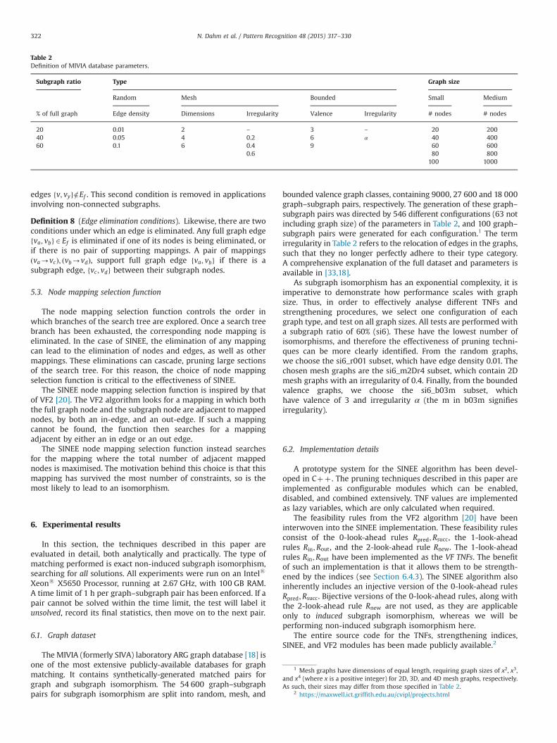
6.3.2. Percentage of extra statesSubgraph isomorphism detection is most commonly performed

using a depth-first tree search, along with some pruning techni-ques. Given a full graph Gf and a subgraph Gs, there are approxi-mately jVf j!=ðjVf j�jVsjÞ! possible subgraph isomorphisms, each ofwhich is a leaf state on the unpruned search tree. The total numberof states in the entire search tree is at least jVsj higher. The numberof search states explored by the matching algorithm is an effectivemeasure of the implementation-independent computational com-plexity of each technique. However the number of explored statesis not a stable metric unless all graph–subgraph pairs are solved.

The states explored by a subgraph isomorphism detection algo-rithm can be classified as either required or failed. Required states arethose states which have at least one descendant that is a validisomorphism, while all leaf states descending from failed states areinvalid isomorphisms. In order to evaluate the pruning effectivenessof different algorithm configurations, the percentage of extra (failed)states is given. This metric is formally calculated as (Failed States=Required StatesÞ � 100%. So if one test explores 60 states, including45 failed and 15 required, it can be said to have explored 45=15�100%¼ 300% extra states. As the number of required states foundapproaches zero, the percentage of extra states approaches infinity(limRS-0FS=RS� 100%¼1%). Therefore, in cases where no requiredstates are found, we simply use an arbitrarily large value (outside of

100

1000

10000

100000

1 2 3 4 5 6 7 8

Per

cent

age

of e

xtra

sta

tes

(%)

Maximum nN depth

0.1

1

10

100

1 2 3 4 5 6 7 8

Mat

chin

g tim

e (s

)

Maximum nN depth

0.0001

0.001

0.01

0.1

1 2 3 4 5 6 7 8

Mat

chin

g tim

e pe

r sta

te (s

)

Maximum nN depth

1000

10000

100000

1e+06

1 2 3 4 5 6 7 8

Mem

ory

(kB

)

Maximum nN depth

Fig. 3. Matching results as a factor of maximum nN depth, for all nN TNFs.

Table 3Matching results for the SINEE algorithm on the si6_r005_s20 dataset, with variousTNF configurations.

TNFs Extra states (%) Matching time (s) Matching time per state (s)

No TNFs 74 340 0.90 3:53e�5

VF TNFs 4140 0.32 2:23e�4

Degree 7980 0.12 4:40e�5

clusterc 52 260 7.05 3:96e�4

nwalksp 4825 0.94 5:38e�4

N. Dahm et al. / Pattern Recognition 48 (2015) 317–330 323

the plot ranges) to visually show that such cases are significantlyhigher than others.

6.3.3. Matching timeNaturally, the most common benchmark for subgraph iso-

morphism algorithms is the matching time. However the match-ing time is heavily dependent on the implementation, so shouldnot be used as the sole metric in prototype systems.

6.3.4. Computation time per stateThe matching time can be decomposed into the number of

explored states, and the computation time required at each state.By comparing the gradients of both the total matching time, aswell as the computation time per state, over a set of graphs, onecan better ascertain the influences of the computation time perstate and the number of explored states. This metric is formallycalculated as Matching Time=Explored States.

6.3.5. Memory usedThe practicality of all algorithms depend on their spatial

complexity as well as computational complexity. To measure thepractical memory requirements of different configurations, thepeak memory usage is recorded. Note that test pairs are matchedin series, so the memory value is the maximum required for asingle test pair.

6.4. Configuration experiments

In this section, the pruning techniques described in this paper areevaluated, in order to determine the most effective techniques andparameters. The graphs used for these experiments are the

si6_r005_s20 (random graphs with 0.05 edge density and size 20)subset. These graphs are sufficiently small enough to be solvedwithin the time limit without using any TNFs, yet still containenough structural complexity to showcase the effectiveness of themore advanced pruning techniques. For comparison with the tech-niques described in this paper, the results for SINEE with threeregular TNFs, the VF TNFs, and no TNFs, are provided in Table 3.

6.4.1. n-neighbourhood TNFsThe nN TNFs are calculated on nNs of depth n¼ 1;2;…;m, where

m is the maximum nN depth. Fig. 3 shows the results from each ofthe nN TNFs, for maximum nN depth m¼ 1;2;…;8. The pruningpower of these nN TNFs is immediately apparent, as even at justm¼2, three of the four nN TNFs have achieved more pruning thanall of the regular TNFs. As the matching time per state increasesexponentially as the maximum nN depth is increased, the optimummaximum nN depth is confirmed to be two.

The poor performance of nN-nwalkspk is explained by theprocess of forming nNs on directed graphs. An nN is formed byfollowing either in-edges or out-edges, but not both. This often (butnot always) results in the centre node being the only root node(out-edges) or leaf node (in-edges). In such cases, no walks actuallypass through the centre node, however any walks beginning orending at it are counted. On undirected graphs, such issues are notprevalent, and nN-nwalkspk has been shown to perform better thanits regular counterpart [27]. The regular TNF of clustering coefficientis afflicted by a similar issue on directed graphs.

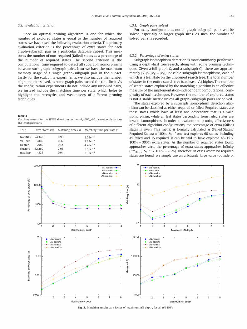
6.4.2. Strengthening indicesThe three strengthening indices, and their nN-strengthened

counterparts are shown in Fig.2pc 4. Comparing the three indices,

Fig. 4. Matching results as a factor of maximum iteration number, for each index, strengthening degree.

N. Dahm et al. / Pattern Recognition 48 (2015) 317–330324

the pruning increase from SI-LI-TI is as was expected. Thematching time per state however, appears to be counter-intuitive.Given that a SI comparison involves a number comparison (4), LIrequires multiple number comparisons, and TI involves a treesearch, it is surprising that the matching time per state is sosimilar between SI/LI/TI. Two hypotheses could explain suchbehaviour. The first is that search tree states near the root stateare less constrained, so take longer to process. Slower but moreeffective pruning techniques may prune away many of theseexpensive states, resulting in an average mainly calculated fromcheap states. The second hypothesis is that, at each state, TIreaches convergence faster than LI, which in turn converges fasterthan SI. This faster convergence results in lower algorithm over-head. By utilising, or drawing inspiration from, focus search [22],an updated implementation of the indices may reduce thisoverhead.

The pruning effectiveness of the tree index is especiallysignificant, as it has reduced the percentage of extra states forthe degree TNF from 7980% to 34%.

As expected, the nN-strengthening improves the pruningeffectiveness of the indices. However, the additional pruningcomes at a significant cost in terms of matching time per state,resulting in a far higher matching time.

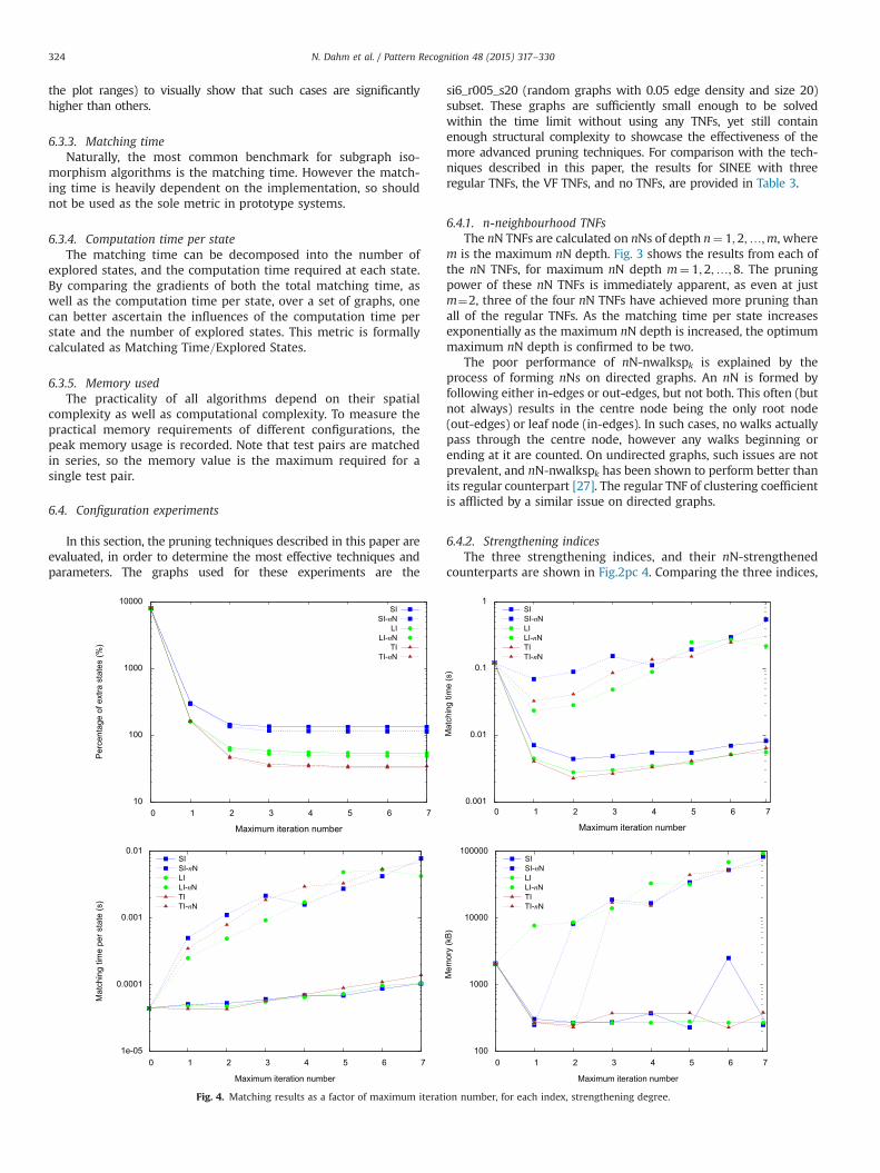
6.4.3. Tree index on all TNFsAs the tree index has been established as the most effective

index, it will be used as the primary index for all subsequentexperiments. In Fig. 5, the tree index is used to propagate all of theTNFs discussed thus far. The maximum nN depth used for the nNTNFs is set to two.

The effect of the tree index is clearly evident on all TNFs. Eventechniques which performed poorly on their own, such as clustercand nN-nwalkspk were significantly improved. The improvementof nN-nwalkspk is especially noteworthy, as it shows how TNFswhich appear to be ineffective, can be strengthened to the pointwhere they become competitive.

The most effective TI-strengthened TNF, in terms of pruningpower, is the VF TNFs. While initially having 4140% extra searchstates, the tree index was able to strengthen the VF TNFs to pruneall but 12% of the extra states. This shows the true potential of theVF TNFs, and helps to explain why the VF2 algorithm has been sosuccessful.

In terms of total matching time, degree is clearly the mostefficient at 0.0022 s per graph–subgraph pair. This is due to ithaving the lowest matching time per state, combined with itscompetitive number of explored states. The pruning effectivenessof degree, combined with the fact that it is inherently calculated inmany algorithms, make it an ideal TNF to add to the implementa-tion of any subgraph isomorphism algorithm. For example, theigraph implementation of VF2 [34] uses degree in addition to the1-look-ahead Rin;Rout rules.

Next after degree, in terms of matching time, are nN-ncountand nN-ecount, with 0.014 and 0.016 s per graph–subgraph pair,respectively. Despite being substantially slower than degree, theresults show the potential of these nN TNFs. As the graph size orcomplexity increases, the pruning difference between degree andthese nN TNFs increases. For example, on the more densesi6_r01_s20 subset, degree explores 5949% extra states, whilenN-ncount explores 4415%. Given larger and more complexgraphs, this pruning advantage enables these nN TNFs to effec-tively compete with, or combine with, cheaper TNFs like degree.

Fig. 5. Matching results as a factor of maximum iteration number, for tree index, strengthening each TNF.

N. Dahm et al. / Pattern Recognition 48 (2015) 317–330 325

Increasing the maximum iteration number has diminishingreturns, with the number of explored states effectively converging ata maximum iteration number of three. Interestingly, for most TNFs,the matching time per state appears unaffected by the maximum

iteration number, despite this requiring ever-deeper tree searches toconfirm node compatibilities.

6.5. Scalability experiments

The experiments in this section evaluate the scalability, andhence the practicality, of the techniques discussed in this paper.The graphs for these experiments are the si6_r001, si6_m2Dr4, andsi6_b03m subsets at all graph sizes contained in the MIVIAdatabase. For each graph type and size, 100 graph–subgraph pairsare to be matched.

6.5.1. Difficulties specific to each graph typeThe three different types of graphs each contain their own

difficulties. For the bounded valence graphs, aside from the irregula-rities, all nodes have exactly the same degree. However for directedgraphs, the degree TNF is generally split into in-degree and out-degree, which are not individually bounded in this database.

The mesh graphs, aside from their irregularities, are highlysymmetric. Even the directed edges of these meshes flow uni-formly from one corner to the opposite. As such, aside fromirregularities, all nodes which are not on the borders haveidentical in-degree and out-degree. The strengthening indicesand nN TNFs are invaluable in these graphs, as they help todescribe nodes by their proximity to irregularities and bordernodes.

The random graphs are of course the most asymmetric, however asthe edge density is fixed, the average degree of nodes increases as the

Table 5Matching results for non-strengthened TNFs on the si6_r001_s20 dataset.

TNFs Extra states (%) Matching time (s) Matching time per state (s)

No TNFs 9700 0.25 3:43e�5

VF TNFs 1240 0.16 1:61e�4

Degree 1193 0.03 3:50e�5

clusterc 9656 2.36 3:24e�4

nwalksp 357 0.05 1:38e�4

nN-ncount 253 0.07 2:94e�4

nN-ecount 257 0.07 2:92e�4

nN-nwalks 216 0.15 6:61e�4

nN-nwalksp 2446 0.97 5:32e�4

Table 4Pruning configurations for practical experiments.

TNFs 1 2 3 4 5 6 7

VF TNFs � � �Degree � � �nN-ncount � � �nN-ecount � � �TI � � � � � � �

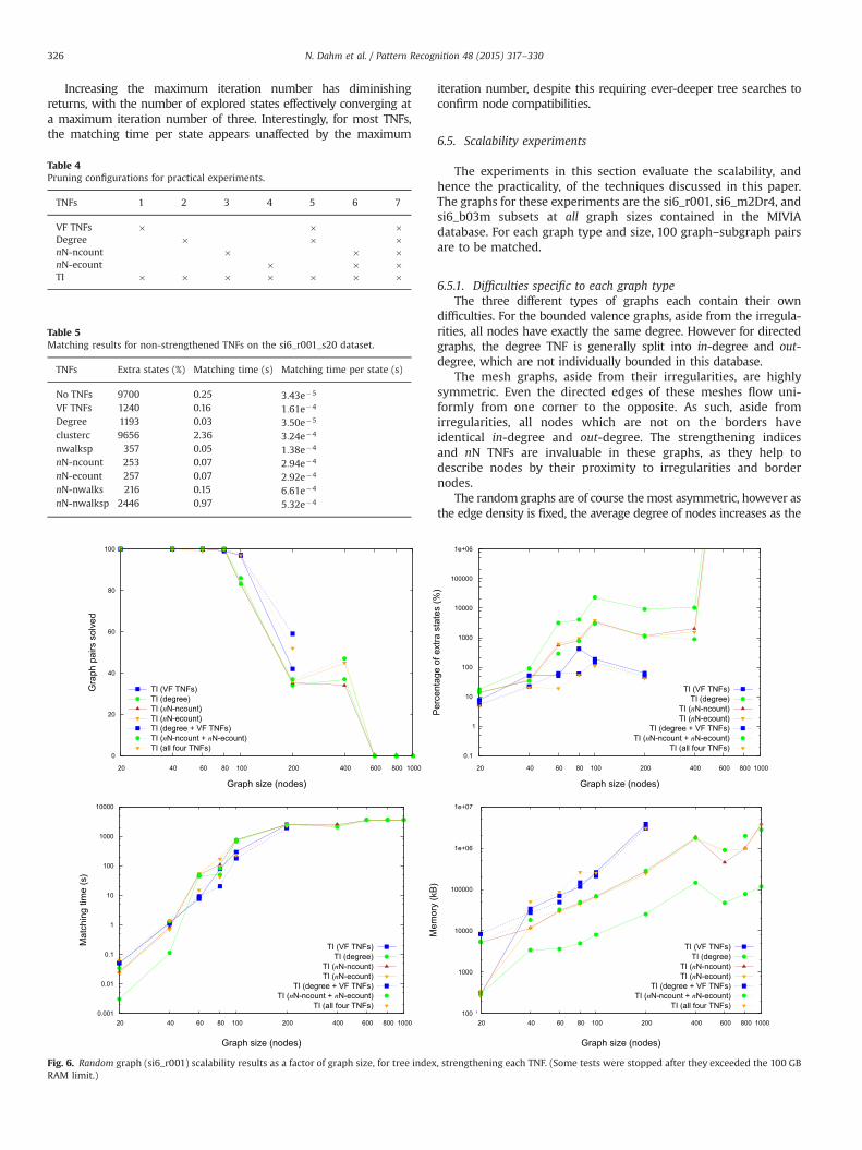
Fig. 6. Random graph (si6_r001) scalability results as a factor of graph size, for tree index, strengthening each TNF. (Some tests were stopped after they exceeded the 100 GBRAM limit.)

N. Dahm et al. / Pattern Recognition 48 (2015) 317–330326

graph size increases. For a graph of size N, there are 0:05N � ðN�1Þedges, leading to an average node degree of 1.9 for a size 20 graph, and9.9 for a size 100 graph. This increase in node degree hinders both thediscriminative power, and computation time, of the strengtheningindices.

6.5.2. Definition of TNF configurationsA number of pruning configurations have been defined, com-

bining TNFs and strengthening indices. These configurations areshown in Table 4. Only strengthened TNFs are used for theseexperiments, as preliminary testing has shown that non-strengthened TNFs cannot complete even the si6_r001_s40 batchwithin the 1 h time limit.

For comparison with the results of these experiments, theresults for non-strengthened TNFs on si6_r001_s20 are given inTable 5. The maximum nN depth used in all configurations is twoand the maximum tree index iteration number is four.

6.5.3. Scalability resultsFigs. 6–8 show the results of the different pruning configura-

tions on graph–subgraph pairs of increasing size from thesi6_r001, si6_m2Dr4, and si6_b03m subsets, respectively. Thefigures clearly show the exponential nature of the subgraphisomorphism problem as the graph size increases.

When comparing the size 20 si6_r001 results in Fig. 6 withthose of the non-strengthened TNFs (Table 5), the benefit ofstrengthening becomes clear, as each strengthened TNF has farfewer extra states to explore than every non-strengthened TNF.

Naturally those tests which utilised all four TNFs had the mosteffective pruning, however all configurations which included theVF TNFs were particularly effective. This is due to the fact that theVF TNFs are technically not pure TNFs, since they are dependent onthe matching state in addition to the graph topology. All otherTNFs discussed in this paper rely solely on the graph topology.

Unfortunately this dependence on the current matching statemeans that some VF TNF values will change (and hence be backedup) every state, instead of only when nodes or edges are elimi-nated. This resulted in a high memory requirement for configura-tions utilising the VF TNFs, to the point where experiments on thesi6_r001 subset with more than 200 nodes exceeded the 100 GBmemory limit. Configurations utilising nN TNFs also used con-siderable memory on the larger tests, however the gradient of theincrease was significantly lower, similar to that of degree.

The degree TNF was, by far, the most efficient in terms ofboth memory usage and matching time per state, with allcompetitors using 10� more memory and taking 10� longerper state. However the lack of pruning power (random graphshad 91% extra states at size 40, rising to 23 141% at size 100)prevented degree from maintaining an ideal matching time.Aside from degree, the other configurations have a similarmatching time per state, generally with a factor of less than5� between them all.

In terms of the total matching time, the combination of degreeand VF TNFs comes out in front for larger graph sizes. These twoTNFs compliment each other well, and since neither is too slowper state, the overall result is impressive.

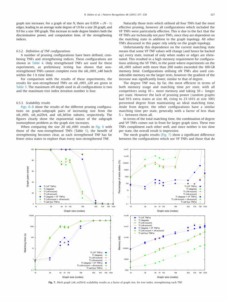
The mesh graphs results (Fig. 7) show a significant differencebetween the configurations which use VF TNFs and those that do

Fig. 7. Mesh graph (si6_m2Dr4) scalability results as a factor of graph size, for tree index, strengthening each TNF.

N. Dahm et al. / Pattern Recognition 48 (2015) 317–330 327

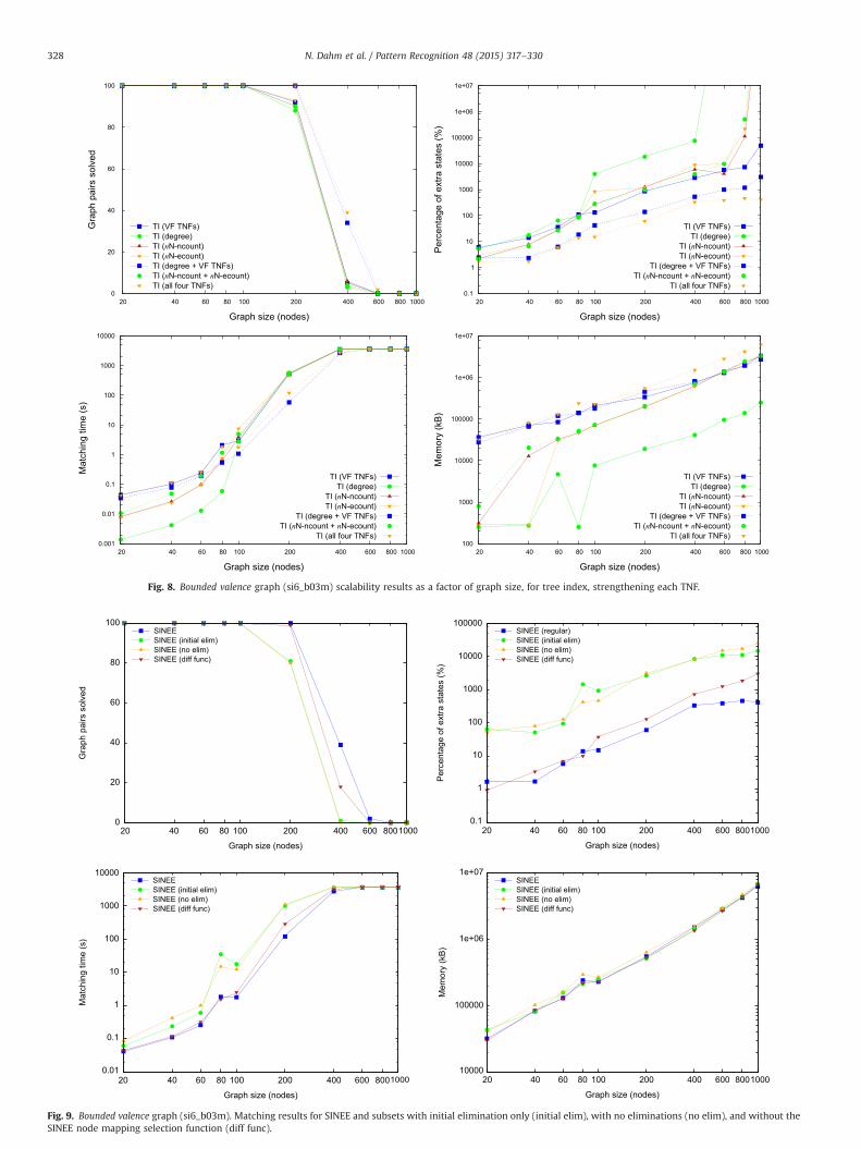
Fig. 8. Bounded valence graph (si6_b03m) scalability results as a factor of graph size, for tree index, strengthening each TNF.

0

20

40

60

80

100

20 40 60 80 100 200 400 600 8001000

Gra

ph p

airs

sol

ved

Graph size (nodes)

SINEESINEE (initial elim)SINEE (no elim)SINEE (diff func)

0.1

1

10

100

1000

10000

100000

20 40 60 80 100 200 400 600 8001000

Per

cent

age

of e

xtra

sta

tes

(%)

Graph size (nodes)

SINEE (regular)SINEE (initial elim)SINEE (no elim)SINEE (diff func)

0.01

0.1

1

10

100

1000

10000

20 40 60 80 100 200 400 600 8001000

Mat

chin

g tim

e (s

)

Graph size (nodes)

SINEESINEE (initial elim)SINEE (no elim)SINEE (diff func)

10000

100000

1e+06

1e+07

20 40 60 80 100 200 400 600 8001000

Mem

ory

(kB

)

Graph size (nodes)

SINEESINEE (initial elim)SINEE (no elim)SINEE (diff func)

Fig. 9. Bounded valence graph (si6_b03m). Matching results for SINEE and subsets with initial elimination only (initial elim), with no eliminations (no elim), and without theSINEE node mapping selection function (diff func).

N. Dahm et al. / Pattern Recognition 48 (2015) 317–330328

not. Configurations utilising the VF TNFs took almost 10� longerper state on these graphs. However for graph sizes up to 400, theyexplored less than 400% extra states, while other configurationsexplored over 10 000% on all graph sizes larger than 16. This islikely due to the fact that the VF TNFs encode the matching state inaddition to the graph structure, which is highly symmetric onmesh graphs.

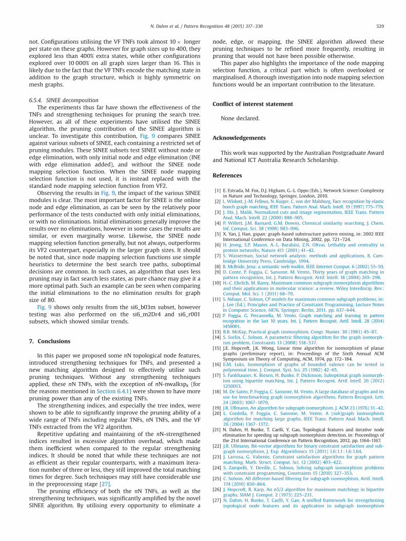
6.5.4. SINEE decompositionThe experiments thus far have shown the effectiveness of the

TNFs and strengthening techniques for pruning the search tree.However, as all of these experiments have utilised the SINEEalgorithm, the pruning contribution of the SINEE algorithm isunclear. To investigate this contribution, Fig. 9 compares SINEEagainst various subsets of SINEE, each containing a restricted set ofpruning modules. These SINEE subsets test SINEE without node oredge elimination, with only initial node and edge elimination (INEwith edge elimination added), and without the SINEE nodemapping selection function. When the SINEE node mappingselection function is not used, it is instead replaced with thestandard node mapping selection function from VF2.

Observing the results in Fig. 9, the impact of the various SINEEmodules is clear. The most important factor for SINEE is the onlinenode and edge elimination, as can be seen by the relatively poorperformance of the tests conducted with only initial eliminations,or with no eliminations. Initial eliminations generally improve theresults over no eliminations, however in some cases the results aresimilar, or even marginally worse. Likewise, the SINEE nodemapping selection function generally, but not always, outperformsits VF2 counterpart, especially in the larger graph sizes. It shouldbe noted that, since node mapping selection functions use simpleheuristics to determine the best search tree paths, suboptimaldecisions are common. In such cases, an algorithm that uses lesspruning may in fact search less states, as pure chance may give it amore optimal path. Such an example can be seen when comparingthe initial eliminations to the no elimination results for graphsize of 80.

Fig. 9 shows only results from the si6_b03m subset, howevertesting was also performed on the si6_m2Dr4 and si6_r001subsets, which showed similar trends.

7. Conclusions

In this paper we proposed some nN topological node features,introduced strengthening techniques for TNFs, and presented anew matching algorithm designed to effectively utilise suchpruning techniques. Without any strengthening techniquesapplied, these nN TNFs, with the exception of nN-nwalkspk (forthe reasons mentioned in Section 6.4.1) were shown to have morepruning power than any of the existing TNFs.

The strengthening indices, and especially the tree index, wereshown to be able to significantly improve the pruning ability of awide range of TNFs including regular TNFs, nN TNFs, and the VFTNFs extracted from the VF2 algorithm.

Repetitive updating and maintaining of the nN-strengthenedindices resulted in excessive algorithm overhead, which madethem inefficient when compared to the regular strengtheningindices. It should be noted that while these techniques are notas efficient as their regular counterparts, with a maximum itera-tion number of three or less, they still improved the total matchingtimes for degree. Such techniques may still have considerable usein the preprocessing stage [27].

The pruning efficiency of both the nN TNFs, as well as thestrengthening techniques, was significantly amplified by the novelSINEE algorithm. By utilising every opportunity to eliminate a

node, edge, or mapping, the SINEE algorithm allowed thesepruning techniques to be refined more frequently, resulting inpruning that would not have been possible otherwise.

This paper also highlights the importance of the node mappingselection function, a critical part which is often overlooked ormarginalised. A thorough investigation into node mapping selectionfunctions would be an important contribution to the literature.

Conflict of interest statement

None declared.

Acknowledgements

This work was supported by the Australian Postgraduate Awardand National ICT Australia Research Scholarship.

References

[1] E. Estrada, M. Fox, D.J. Higham, G.-L. Oppo (Eds.), Network Science: Complexityin Nature and Technology, Springer, London, 2010.

[2] L. Wiskott, J.-M. Fellous, N. Kuiger, C. von der Malsburg, Face recognition by elasticbunch graph matching, IEEE Trans. Pattern Anal. Mach. Intell. 19 (1997) 775–779.

[3] J. Shi, J. Malik, Normalized cuts and image segmentation, IEEE Trans. PatternAnal. Mach. Intell. 22 (2000) 888–905.

[4] P. Willett, J.M. Barnard, G.M. Downs, Chemical similarity searching, J. Chem.Inf. Comput. Sci. 38 (1998) 983–996.

[5] X. Yan, J. Han, gspan: graph-based substructure pattern mining, in: 2002 IEEEInternational Conference on Data Mining, 2002, pp. 721–724.

[6] H. Jeong, S.P. Mason, A.-L. Barabási, Z.N. Oltvai, Lethality and centrality inprotein networks, Nature 411 (2001) 41–42.

[7] S. Wasserman, Social network analysis: methods and applications, 8, Cam-bridge University Press, Cambridge, 1994.

[8] B. McBride, Jena: a semantic web toolkit, IEEE Internet Comput. 6 (2002) 55–59.[9] D. Conte, P. Foggia, C. Sansone, M. Vento, Thirty years of graph matching in

pattern recognition, Int. J. Pattern Recognit. Artif. Intell. 18 (2004) 265–298.[10] H.-C. Ehrlich, M. Rarey, Maximum common subgraph isomorphism algorithms

and their applications in molecular science: a review, Wiley Interdiscip. Rev.:Comput. Mol. Sci. 1 (2011) 68–79.

[11] S. Ndiaye, C. Solnon, CP models for maximum common subgraph problems, in:J. Lee (Ed.), Principles and Practice of Constraint Programming, Lecture Notesin Computer Science, 6876, Springer, Berlin, 2011, pp. 637–644.

[12] P. Foggia, G. Percannella, M. Vento, Graph matching and learning in patternrecognition in the last 10 years, Int. J. Pattern Recognit. Artif. Intell. 28 (2014)1450001.

[13] B.B. McKay, Practical graph isomorphism, Congr. Numer. 30 (1981) 45–87.[14] S. Sorlin, C. Solnon, A parametric filtering algorithm for the graph isomorph-

ism problem, Constraints 13 (2008) 518–537.[15] J.E. Hopcroft, J.K. Wong, Linear time algorithm for isomorphism of planar

graphs (preliminary report), in: Proceedings of the Sixth Annual ACMSymposium on Theory of Computing, ACM, 1974, pp. 172–184.

[16] E.M. Luks, Isomorphism of graphs of bounded valence can be tested inpolynomial time, J. Comput. Syst. Sci. 25 (1982) 42–65.

[17] S. Fankhauser, K. Riesen, H. Bunke, P. Dickinson, Suboptimal graph isomorph-ism using bipartite matching, Int. J. Pattern Recognit. Artif. Intell. 26 (2012)1250013.

[18] M. De Santo, P. Foggia, C. Sansone, M. Vento, A large database of graphs and itsuse for benchmarking graph isomorphism algorithms, Pattern Recognit. Lett.24 (2003) 1067–1079.

[19] J.R. Ullmann, An algorithm for subgraph isomorphism, J. ACM 23 (1976) 31–42.[20] L. Cordella, P. Foggia, C. Sansone, M. Vento, A (sub)graph isomorphism

algorithm for matching large graphs, IEEE Trans. Pattern Anal. Mach. Intell.26 (2004) 1367–1372.

[21] N. Dahm, H. Bunke, T. Caelli, Y. Gao, Topological features and iterative nodeelimination for speeding up subgraph isomorphism detection, in: Proceedings ofthe 21st International Conference on Pattern Recognition, 2012, pp. 1164–1167.

[22] J.R. Ullmann, Bit-vector algorithms for binary constraint satisfaction and sub-graph isomorphism, J. Exp. Algorithmics 15 (2011) 1.6:1.1–1.6:1.64.

[23] J. Larrosa, G. Valiente, Constraint satisfaction algorithms for graph patternmatching, Math. Struct. Comput. Sci. 12 (2002) 403–422.

[24] S. Zampelli, Y. Deville, C. Solnon, Solving subgraph isomorphism problemswith constraint programming, Constraints 15 (2010) 327–353.

[25] C. Solnon, All different-based filtering for subgraph isomorphism, Artif. Intell.174 (2010) 850–864.

[26] J. Hopcroft, R. Karp, An n5/2 algorithm for maximum matchings in bipartitegraphs, SIAM J. Comput. 2 (1973) 225–231.

[27] N. Dahm, H. Bunke, T. Caelli, Y. Gao, A unified framework for strengtheningtopological node features and its application to subgraph isomorphism

N. Dahm et al. / Pattern Recognition 48 (2015) 317–330 329

detection, in: W.G. Kropatsch, N.M. Artner, Y. Haxhimusa, X. Jiang (Eds.),Graph-Based Representations in Pattern Recognition, Lecture Notes in Com-puter Science, 7877, Springer, Berlin, 2013, pp. 11–20.

[28] H.L. Morgan, The generation of a unique machine description for chemicalstructures—a technique developed at chemical abstracts service, J. Chem. Doc.5 (1965) 107–113.

[29] H.W. Kuhn, The Hungarian method for the assignment problem, Naval Res.Logist. Q. 2 (1955) 83–97.

[30] B. Weisfeiler, A.A. Lehman, A reduction of a graph to a canonical form and analgebra arising during this reduction, Nauchno-Tech. Inf. (1968) 12–16 (inRussian).

[31] N. Shervashidze, K.M. Borgwardt, Fast subtree kernels on graphs, in: Y. Bengio,D. Schuurmans, J. Lafferty, C.K.I. Williams, A. Culotta (Eds.), Advances in NeuralInformation Processing Systems, vol. 22, 2009, pp. 1660–1668.

[32] N. Shervashidze, P. Schweitzer, E.J. van Leeuwen, K. Mehlhorn, K.M. Borgwardt,Weisfeiler–Lehman graph kernels, J. Mach. Learn. Res. 12 (2011) 2539–2561.

[33] P. Foggia, C. Sansone, M. Vento, A database of graphs for isomorphism andsub-graph isomorphism benchmarking, in: Proceedings of the 3rd IAPR-TC15Workshop on Graph-based Representations in Pattern Recognition, 2001,pp. 176–187.

[34] G. Csardi, T. Nepusz, The igraph software package for complex networkresearch, InterJ. Complex Syst. (2006) 1–9.

Nicholas Dahm is a Ph.D. student in the School of Engineering, Griffith University, Australia. He received his B.IT (Hons.) in 2009 from Griffith University. His primaryresearch areas are Computer Vision and Graph Matching.

Horst Bunke received his Ph.D in 1979 from the University of Erlangen, Germany. Since then he has served on numerous editorial boards, received the King-Sun Fu Prize in2010, and is ranked as one of the 150 most prolific authors, according to the DBLP Computer Science Bibliography. Currently, he is an emeritus Professor at the University ofBern, Switzerland.

Terry Caelli received his Ph.D in 1975 from the University of Newcastle, Australia. He has been a prominent member of the research community and has held Professorpositions in Germany, Canada, and Australia. His research interests include computer vision and machine learning for biomedical technologies and environmentalmonitoring.

Yongsheng Gao received B.Sc. and M.Sc. degrees in Electronic Engineering from Zhejiang University, China, in 1985 and 1988, respectively, and a Ph.D. degree in ComputerEngineering from Nanyang Technological University, Singapore. Currently, he is a Professor at the School of Engineering, Griffith University, Australia. His research interestsinclude face recognition, biometrics, image retrieval, computer vision, and pattern recognition.

N. Dahm et al. / Pattern Recognition 48 (2015) 317–330330