Embed Size (px)
Citation preview
EFFICIENT MACHINE LEARNING USING PARTITIONED RESTRICTED
BOLTZMANN MACHINES
by
Hasari Tosun
A dissertation submitted in partial fulfillmentof the requirements for the degree
of
Doctor of Philosophy
in
Computer Science
MONTANA STATE UNIVERSITYBozeman, Montana
May, 2016

c© COPYRIGHT
by
Hasari Tosun
2016
All Rights Reserved

ii
DEDICATION
To Suzan, my dear wife

iii
ACKNOWLEDGEMENTS
I would like to thank my advisor, Dr. John Sheppard for his staunch support
throughout my research at Montana State University. At the times when I was about
to give it up, he always encouraged and pushed me to excel. Without his guidance,
this research would not have been possible.
I would also like to thank my committee members, John Paxton, Rocky Ross,
and Clem Izurieta for their helpful comments and advice, and to thank the members
of the Numerical Intelligent Systems Laboratory at Montana State University for
their comments and advice during the development of this work. Thanks too to Ben
Mitchell at John Hopkins University for his collaboration.
Finally, I would like to thank my wife for supporting me during the development
of this work. Suzan released me of other duties as I worked on my research. My
children, Sundus, Eyub and Yakob, are too little to understand what the PhD is.
Their constant question was “when will your school be done?” You were patient with
me. Now that my work is complete, I will share it with you in time.
iv
TABLE OF CONTENTS
1. INTRODUCTION ........................................................................................1
1.1 Motivation .............................................................................................11.2 Contributions.........................................................................................31.3 Organization ..........................................................................................41.4 Notation ................................................................................................5
2. BACKGROUND...........................................................................................6
2.1 Boltzmann Distribution ..........................................................................62.2 Restricted Boltzmann Machine.............................................................. 11
2.2.1 Inference in RBM: Conditional Probability...................................... 142.2.2 Training RBM: Stochastic Gradient Descent.................................... 162.2.3 Contrastive Divergence .................................................................. 19
2.3 Autoencoders ....................................................................................... 222.4 Deep Learning...................................................................................... 232.5 Spatial and Temporal Feature Analysis .................................................. 26
2.5.1 Variograms.................................................................................... 272.5.2 Autocorrelation and Correlograms .................................................. 282.5.3 Distributed Stochastic Neighbor Embedding.................................... 302.5.4 Dynamic Time Warping ................................................................. 32
3. RELATED WORK ..................................................................................... 35
3.1 Sampling Methods................................................................................ 353.2 Restricted Boltzmann Machines ............................................................ 373.3 Deep Learning...................................................................................... 393.4 Dropout............................................................................................... 433.5 Partitioned Model Learning .................................................................. 443.6 Temporal Classification......................................................................... 46
4. PARTITIONED LEARNING....................................................................... 48
4.1 Data Partitioning Theory...................................................................... 484.2 Partitioned Learning Algorithm............................................................. 514.3 Partitioned Restricted Boltzmann Machines ........................................... 554.4 Experimental Setup .............................................................................. 604.5 Results ................................................................................................ 624.6 Conclusion ........................................................................................... 68
v
TABLE OF CONTENTS – CONTINUED
5. PARTITIONED DISCRIMINATIVE NETWORKS....................................... 70
5.1 Discriminative Restricted Boltzmann Machines ...................................... 705.2 Discriminative Partitioned Restricted Boltzmann Machines..................... 725.3 Experimental Design ............................................................................ 765.4 Results ................................................................................................ 775.5 Conclusion ........................................................................................... 81
6. PARTITIONED DEEP BELIEF NETWORKS............................................. 83
6.1 Deep Belief Networks with Partitioned Restricted Boltz-mann Machines .................................................................................... 83
6.2 Analysis of Spatial Features .................................................................. 886.3 Experimental Setup .............................................................................. 916.4 Results ................................................................................................ 926.5 Discussion............................................................................................ 99
7. TIME SERIES CLASSIFICATION VIA PARTITIONED NETWORKS....... 104
7.1 Time Series Classification ................................................................... 1047.2 Temporal Restricted Boltzmann Machines ........................................... 1067.3 Partitioned Restricted Boltzmann Machines ......................................... 1097.4 Experimental Setup ............................................................................ 1107.5 Results .............................................................................................. 1127.6 Conclusion ......................................................................................... 113
8. SUMMARY AND CONCLUSIONS............................................................ 115
8.1 Summary of Contributions .................................................................. 1158.1.1 Partitioned Learning .................................................................... 1158.1.2 Computational Efficiency ............................................................. 1158.1.3 Efficient Classification .................................................................. 1168.1.4 Preserving Spatially Local Features............................................... 1168.1.5 Sparsity ...................................................................................... 1168.1.6 Time Series Classification............................................................. 117
8.2 Publications ....................................................................................... 1178.3 Future Work ...................................................................................... 118
REFERENCES CITED.................................................................................. 121

vi
TABLE OF CONTENTS – CONTINUED
APPENDICES .............................................................................................. 129
APPENDIX A: Variances .............................................................................. 130
APPENDIX B: Correlations .......................................................................... 142
vii
LIST OF TABLESTable Page
4.1 Training Characteristics....................................................................... 63
4.2 Training Characteristics wrt Learning Rate........................................... 63
4.3 Training Characteristics wrt Learning Rate........................................... 64
4.4 Overlapping Partitions......................................................................... 64
4.5 Non-overlapping vs. Overlapping Partitions .......................................... 65
4.6 10-Fold Cross Validation Results .......................................................... 65
4.7 Training Iterations .............................................................................. 67
4.8 Training Characteristics with NIST dataset .......................................... 67
4.9 Reconstruction Error per Character...................................................... 69
5.1 Classification Accuracy Rates............................................................... 78
5.2 Classification F1 Scores ....................................................................... 79
5.3 Partitioned-RBM Classification Accuracy ............................................ 79
5.4 Classification Accuracy Rates with samples........................................... 80
5.5 Classification Accuracy Rates with iterations ........................................ 81
6.1 Reconstruction Errors.......................................................................... 94
6.2 Reconstruction Errors for 2-layer DBN ................................................. 94
7.1 Partitioned-RBM configuration .......................................................... 111
7.2 Time Series Classification Accuracy.................................................... 112
7.3 Classification Accuracy with Repeated Patterns of FaceAll .................. 113
7.4 Subsequence Classification Accuracy with Repeated Pat-terns of FaceAll ................................................................................. 113
viii
LIST OF FIGURESFigure Page
2.1 Micro states of two-partitions system with three distin-guishable particles .................................................................................7
2.2 Energy levels or occupation numbers of N particles .................................8
2.3 Restricted Boltzmann Machine............................................................. 12
2.4 CD Markov Chain ............................................................................... 21
2.5 Three-layer Deep Belief Network .......................................................... 25
2.6 Three-layer Deep Belief Network: Training - Last Layer......................... 26
2.7 t-SNE Embedding of the MNIST Dataset ............................................. 32
4.1 4× 4-pixels image data........................................................................ 49
4.2 Quadtree partitioning .......................................................................... 50
4.3 A sample RBM with no splits .............................................................. 52
4.4 A sample RBM with two splits............................................................. 53
4.5 Example partitioning approach for an RBM.......................................... 56
4.6 RBM With Overlapping Partitions ....................................................... 59
4.7 Sample MNIST Images ........................................................................ 60
4.8 Original vs. Reconstructed Images ....................................................... 66
4.9 Reconstruction Error vs. Training Samples .......................................... 66
5.1 Class RBM Network ............................................................................ 71
5.2 Discriminative Partitioned RBM .......................................................... 73
6.1 Variogram and mean-correlation plots for the MNIST............................ 90
6.2 Sample images from the MNIST dataset. .............................................. 93
6.3 Variograms: labels 0, 5 and 9. .............................................................. 96
6.4 Correlations: labels 0, 5 and 9.............................................................. 97
6.5 Hidden node activations: 15 iterations .................................................. 97
ix
LIST OF FIGURES – CONTINUEDFigure Page
6.6 MNIST t-SNE mappings...................................................................... 98
6.7 Hidden node activations: Partitions...................................................... 99
7.2 RBM with Feedforward...................................................................... 108
7.3 Partitioned Time Series ..................................................................... 110
A.1 Variogram: Label 0 ........................................................................... 132
A.2 Variogram: Label 1 ........................................................................... 133
A.3 Variogram: Label 2 ........................................................................... 134
A.4 Variogram: Label 3 ........................................................................... 135
A.5 Variogram: Label 4 ........................................................................... 136
A.6 Variogram: Label 5 ........................................................................... 137
A.7 Variogram: Label 6 ........................................................................... 138
A.8 Variogram: Label 7 ........................................................................... 139
A.9 Variogram: Label 8 ........................................................................... 140
A.10 Variogram: Label 9 ........................................................................... 141
B.1 Mean Correlation: Label 0 ................................................................. 144
B.2 Mean Correlation: Label 1 ................................................................. 145
B.3 Mean Correlation: Label 2 ................................................................. 146
B.4 Mean Correlation: Label 3 ................................................................. 147
B.5 Mean Correlation: Label 4 ................................................................. 148
B.6 Mean Correlation: Label 5 ................................................................. 149
B.7 Mean Correlation: Label 6 ................................................................. 150
B.8 Mean Correlation: Label 7 ................................................................. 151
B.9 Mean Correlation: Label 8 and 9........................................................ 152
x
LIST OF ALGORITHMSAlgorithm Page
2.1 GRADIENT-DESCENT(J(θ), α) ..................................................... 16
2.2 STOCHASTIC-GRADIENT-DESCENT(J(θ), α) ........................... 17
2.3 CD-1(xi, α) ....................................................................................... 21
2.4 DTW(s, t) ......................................................................................... 34
4.1 PARTITIONED-LEARNING(D, π, stages, ρ) ................................. 54
4.2 PARTITIONED-RBM(L, nvisible, nhidden) .................................. 57
4.3 PARTITIONED-RBM-UPDATE(l, X , W, b, c) .............................. 57
4.4 PARTITIONED-RBM-INIT(l, W, b, c) .......................................... 58
5.1 PARTITIONED-DISC-RBM ........................................................... 76
xi
ABSTRACT
Restricted Boltzmann Machines (RBM) are energy-based models that are usedas generative learning models as well as crucial components of Deep Belief Networks(DBN). The most successful training method to date for RBMs is Contrastive Diver-gence. However, Contrastive Divergence is inefficient when the number of features isvery high and the mixing rate of the Gibbs chain is slow.
We develop a new training method that partitions a single RBM into multipleoverlapping atomic RBMs. Each partition (RBM) is trained on a section of theinput vector. Because it is partitioned into smaller RBMs, all available data canbe used for training, and individual RBMs can be trained in parallel. Moreover, asthe number of dimensions increases, the number of partitions can be increased toreduce runtime computational resource requirements significantly. All other recentlydeveloped methods for training RBMs suffer from some serious disadvantage underbounded computational resources; one is forced to either use a subsample of thewhole data, run fewer iterations (early stop criterion), or both. Our Partitioned-RBM method provides an innovative scheme to overcome this shortcoming.
By analyzing the role of spatial locality in Deep Belief Networks (DBN), we showthat spatially local information becomes diffused as the network becomes deeper.We demonstrate that deep learning based on partitioning of Restricted BoltzmannMachines (RBMs) is capable of retaining spatially local information. As a result, inaddition to computational improvement, reconstruction and classification accuracy ofthe model is also improved using our Partitioned-RBM training method.
1
CHAPTER 1
INTRODUCTION
In this chapter, we present the motivation for developing Partitioned Restricted
Boltzmann Machines (Partitioned-RBM), specifically in applications where the com-
putational resources are bounded. After a brief introduction to the characteristics of
current datasets and the limitation of RBMs, we introduce Partitioned-RBM as an
alternative training method that addresses computational requirements. Then, we
summarize our major contributions and conclude with an overview of each section of
this dissertation.
1.1 Motivation
As the volume of data is increasing exponentially, the corresponding need for
efficient learning algorithms is also increasing. In addition to the traditional Internet,
in the Internet of Things (IoT) where a variety of smart devices are connected to
each other and to the Internet, the volume of data generated is immense. There are
some basic characteristics of recent data: 1) it is collected from many sources, 2) it is
very high dimensional, 3) it is complex, having many latent variables with complex
distributions, and 4) it is spatio-temporal. Representing such data efficiently and
developing computationally efficient algorithms is a challenging task. Most of the
training algorithms for learning are based on gradient descent with data likelihood
objective functions that are intractable to compute [1].
An example of data generated by users and sensors is images. Image pixel resolu-
tion is increasing continuously. An image taken by a cheaper camera with 2048×1536
2
pixels resolution has 3.1 million total pixels. Thus, without any preprocessing, the
dimension of the image is 3.1 million. If one were to construct a neural network,
the input layer would need to have 3.1 million neurons. If the network had a single
hidden layer, also with 3.1 million neurons, then propagating information from one
layer to next would involve 9 × 10¹² calculations. This is even more prohibitive
when deep neural networks with multiple hidden layers are used. As of 2010, Google
indexed approximately 10 billion images [2]. Current machine learning methods can
not handle such datasets when the number of images are on the order of billions.
An immediate solution to overcome the time complexity of training algorithms
is to distribute learning on many nodes for processing. However, in current Deep
Neural Network (DBN) algorithms, to accomplish an optimization task on multiple
machines, a central node is needed for communicating intermediate results. As a
result, the communication becomes a bottleneck.
In addition to training and inference time complexity, representation is an issue:
what is the best model to represent and process features effectively? The performance
of machine learning methods is dependent on the choice of data representation. Re-
cent studies show a representation that maximizes sparsity has properties of the
receptive fields of simple cells in the mammalian primary visual cortex; receptive
fields are spatially localized, oriented, and selective to structure at different spatial
scales [3]. In a sparse representation, most of the extracted features will be sensitive
to variations in data; thus, sparseness is a key component of good representation [4].
Moreover, there is a need for distributed representations where a concept is repre-
sented by many neurons and a neuron is involved in many concepts. Energy-based
models such as Markov Random Fields, Boltzmann Machines, and Autoencoders have
gained significant success. However, these algorithms, although tractable, are slow if
data dimensionality is very high.
3
We implemented a partitioned Restricted Boltzmann Machine (RBM) and trained
an individual RBM separately [5]. We realized that partitioned RBMs are not only
more accurate in terms of their generative power, they are also fast. Our results shows
that they are also very accurate in terms of their discriminative power, namely in a
classification task. As a result, a learning method with many partitioned small RBMs
is more accurate and efficient. Training Partitioned-RBMs involves several partition
steps. In each step, the RBM is partitioned into multiple RBMs. We demonstrate
that Partitioned-RBMs have better representation and computational performance
as compared to monolithic RBMs.
1.2 Contributions
In this section, we briefly list the major contributions of this dissertation. A more
comprehensive summary is given in Chapter 8.
• We develop a novel partitioned learning method in Chapter 4 . Partitioned-
RBMs enable data-independent parallelization and since each sub partition has
fewer nodes and weights to be updated, our method has better computational
performance. We find that Partitioned-RBMs possess natural sparsity charac-
teristics because each Partitioned-RBMs are trained on localized regions of the
dataset.
• We show in Chapter 5 that Partitioned-RBMs can be used efficiently as discrim-
inative models with better performance in terms of computational requirements.
• We demonstrate in Chapter 6 that Partitioned-RBMs can be used effectively as
part of Deep Belief Networks while preserving spatially local features.
4
• In Chapter 7, we apply Partitioned-RBMs to time series classification datasets,
and show that Partitioned-RBMs perform well in classifying time series with
high dimensions.
1.3 Organization
This section describes the organization of the remaining chapters of the disserta-
tion and gives a brief overview of the focus of each chapter.
In Chapter 2, we review the background work common to this line of research.
We describe concepts related to energy-based models. Most energy-based models
rely on the Boltzmann distribution, the partition function, and free energy. Thus, we
describe these concepts and derive energy functions for the Boltzmann distribution.
We then describe Constrastive Divergence (CD) algorithm in detail. This discussion
is followed by an introduction on deep learning and Deep Belief Networks (DBN).
Finally, we introduce tools for evaluating spatially local features. These tools will be
used in analyzing data and derived features in the subsequent.
In Chapter 3, we review the literature of Deep Belief Networks, Boltzmann Re-
stricted Machines and related approaches.
In Chapter 4, we discuss partitioning theory and develop a generic partitioned
based training procedure. We describe how data and model is partitioned. We then
develop Partitioned Restricted Boltzmann Machine (PRBM). Applying to an image
dataset, we analyze performance characteristics of Partitioned-RBMs.
In Chapter 5, we develop a discriminative version of Partitioned-RBM. We ap-
ply our model to an image classification task and show classification accuracy and
computational performance of the model.

5
In Chapter 6, we assess the characteristics of Partitioned-RBMs in the context of
deep learning. Specifically, we carry out analysis on how Partitioned-RBMs used in
DBNs can exploit spatially local features with performance improvements.
In Chapter 7, we apply Partitioned-RBMs to temporal datasets. We demonstrate
that Partitioned-RBMs can classify time series effectively.
In Chapter 8, we draw conclusions and summarize the contributions resulting from
this work. We list future work and conclude with a list of published papers resulting
from this research.
1.4 Notation
All notation used throughout this thesis is described in this section.
a, b, c, w lowercase italic symbols for scalarsa,b, c,x lowercase bold symbols for vectorsW uppercase bold symbols for matricesx> x> denotes transpose of the vector xxi ith element of vector xxi ith row vector of matrix Xxij the ith row and jth column of matrix XX(w), or X denotes random variables
6
CHAPTER 2
BACKGROUND
Today, most of the data generated by humans and devices is unlabeled and of
very high dimension. Methods in deep learning attempt to manage the data flood and
curse of dimensionality by discovering structure and abstractions in the data. Because
of similarities in how physical systems organize, most energy-based neural networks
have become popular. In this chapter, we present the theoretical foundation for
energy-based models. We derive the necessary energy-based mathematical formulas
and present existing related learning methods. We also describe various methods and
tools for analysis of spatial and temporal features.
2.1 Boltzmann Distribution
In this section, we describe the Boltzmann Distribution, as the foundation of statis-
tical mechanics. In statistical mechanics, a certain quantity of matter under thermo-
dynamic study or analysis is called a system. When the thermodynamic system was
viewed as black box, the Austrian physicist Ludwig Boltzmann(1844-1906) thought
of a system in terms of atoms and molecules and described entropy (a measure of the
number of specific ways in which a thermodynamic system may be arranged) in terms
of possible disposition of atoms [6]. Boltzmann characterized thermodynamic systems
with possible arrangements of atoms and molecules. In other words, he examined the
second law of thermodynamics in terms of its possible atomic arrangements. This
line of thinking helped to create the field of statistical mechanics.
7
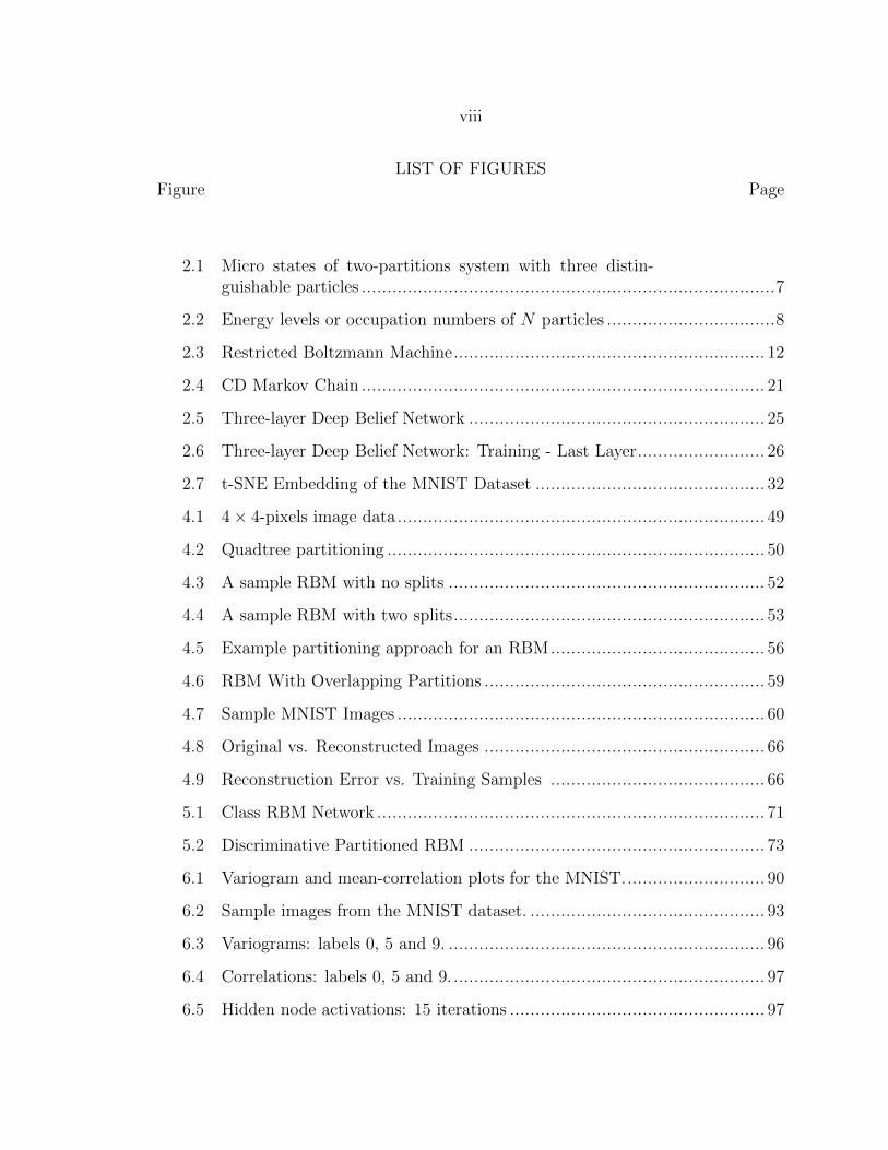
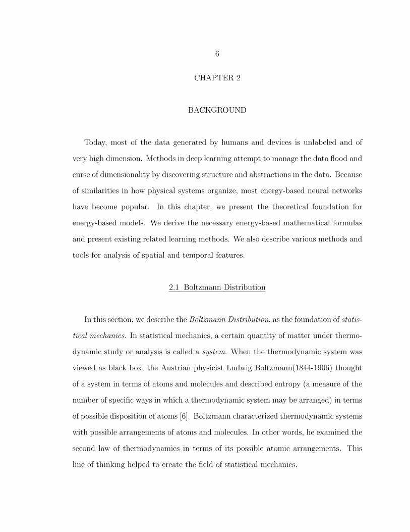
Figure 2.1: Micro states of two-partitions system with three distinguishable particles
Definition 2.1.1. (Microstate) A microstate in statistical mechanics is identified by
“a detailed particle-level description of the system.” For example, microstates for a
system with equal-volume parts and three distinguishable particles has 23 = 8 different
microstates, as illustrated in Figure 2.1.
Definition 2.1.2. (Macrostate) A macrostate in statistical mechanics consists of
a set of microstates that can be described with a relatively small set of variables.
Specifically, a macrostate is a thermodynamic or equilibrium state that can be defined
in terms of variables energy (E), volume (V ), and particle number (n). For example,
8
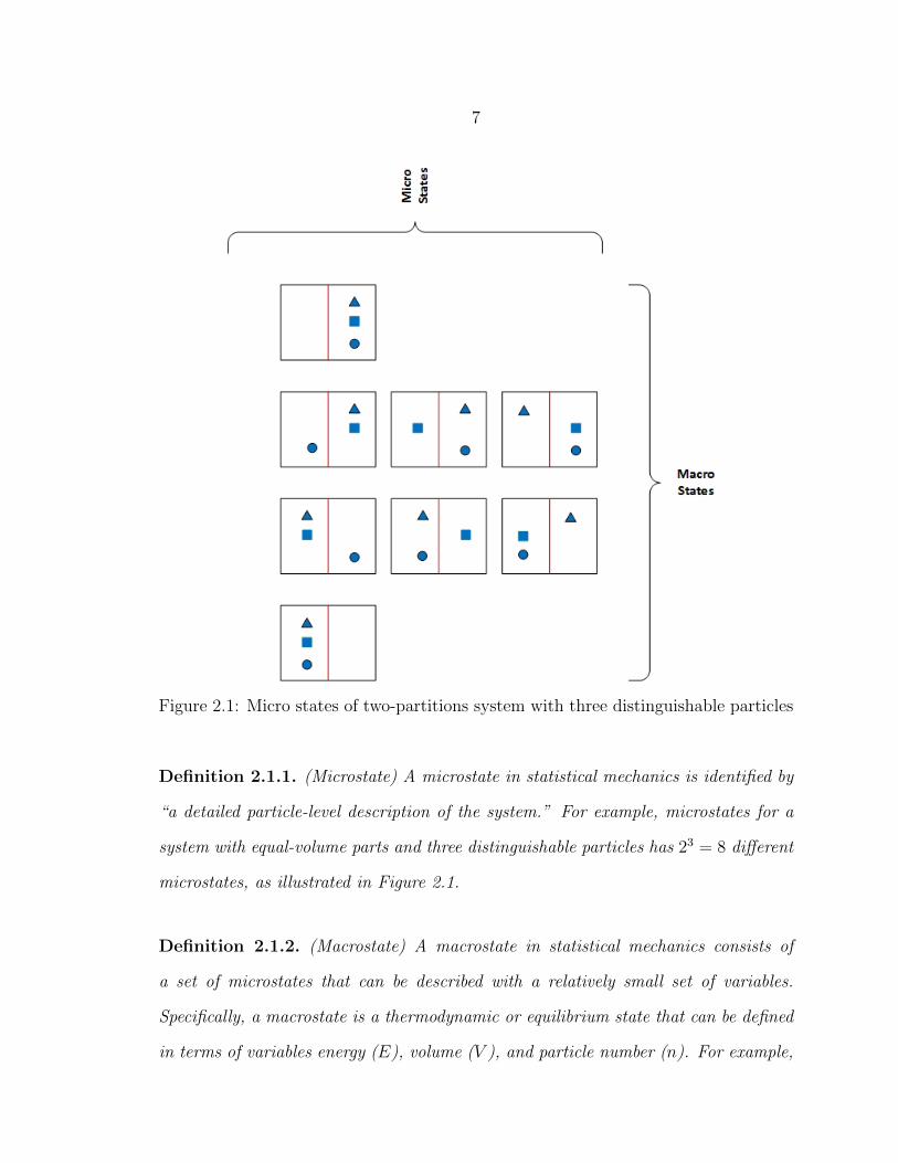
Figure 2.2: Energy levels or occupation numbers of N particles
Figure 2.1, shows four macrostates one of which is a two-sided system where two
particles are in the left partition and one particle is on the right. This macrostate has
three microstates.
Boltzmann defined special macrostates by the number of particles ni that occupy a
particular energy level i. These macro states are also called “occupation numbers.” A
set of occupation numbers, n1, n2..., nj defines a particular macrostate of the system.
Suppose we have n copies of a system in a heat bath as shown in Figure 2.2 where
n is very large. Drawing from n, we want to know how many boxes occupy state i
or energy level i. Since there are an infinite number of states, most of these states
will have zero assignments, and all boxes have the same average energy. Moreover,
assume that the total energy is Etotal = n× E, where E is the average energy. Then,
the number of ways that occupational numbers can be realized is
Ω =n!∏ni=1 ni
.
9
The probability that any given box will be in state i is given by P (i) = ni
n. Thus,
we have following constraints:n∑i=1
P (i) = 1 (2.1)
n∑i=1
niEi = nE (2.2)
where the average energy can be written in terms of probability as E =∑n
i=1 P (i)Ei.
Instead of maximizing Ω, it is easier to maximize the log(Ω). Thus, log(Ω) = log(n!)−∑ni=1 log(ni!). Using Stirling’s approximation, log(n!) ∼= n log(n)− n, we get
log(Ω) ∼= −nn∑i=1
P (i) log(P (i)) (2.3)
Note that, −∑n
i=1 P (i) log(P (i)) is the entropy of a single system. To op-
timize (finding minimum or maximum) Equation 2.3 subject to the constraints
defined in Equation 2.1 and Equation 2.2, we apply Lagrange Multipliers as
−∑n
i=1 P (i) log(P (i)) − α∑n
i=1 P (i) − β∑n
i=1 niEi = 0, where α and β are the La-
grange multipliers. Differentiating the function with respect to P (i), the probability
is obtained as:
P (i) = e−(1+α)e−βEi . (2.4)
The term β is defined in terms of temperature as 1kbT
where kb is the Boltzmann
constant and T is temperature. Historically, e−(1+α) = 1Z
where Z is the partition
function. The partition function is the sum over all the microstates of the system.
In probability theory, it is used as normalization constant. Using the constraint in
10
Equation 2.1, we rewrite the partition function as:
Z(β) =n∑i=1
e−βEi (2.5)
Thus, the probability can be written as:
P (i) =1
Ze−βEi (2.6)
This equation is the Boltzmann Distribution. Z ensures that∑n
i=1 p(i) = 1. The
partition function contains a great deal of information. For example, average energy,
E, can be written as E = −∂ logZ∂β
. The following are important definitions and
equations related to the partition function.
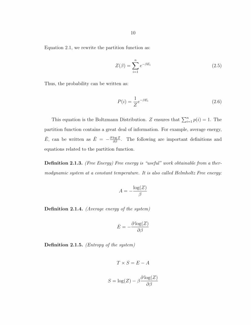
Definition 2.1.3. (Free Energy) Free energy is “useful” work obtainable from a ther-
modynamic system at a constant temperature. It is also called Helmholtz Free energy:
A = − log(Z)
β
Definition 2.1.4. (Average energy of the system)
E = −∂ log(Z)
∂β
Definition 2.1.5. (Entropy of the system)
T × S = E − A
S = log(Z)− β∂ log(Z)
∂β
11
2.2 Restricted Boltzmann Machine
One of the well known approaches for feature representation is the Restricted
Boltzmann Machine (RBM). An RBM is a type of Hopfield net and a restricted
version of the general Boltzmann Machines (BM). A BM is a network of visible and
hidden stochastic binary units where the network is fully connected. On the other
hand, an RBM network is a bi-partite graph where only hidden and visible nodes are
coupled. There are no dependencies among visible nodes or among hidden nodes. The
RBM model was first proposed by Smolensky [7] in 1986. Hinton et al. developed an
algorithm to train a BM in 1985 as a parallel network for constraint satisfaction [8].
As discussed in Section 2.1, in statistical mechanics, the Boltzmann distribution is
the probability of a random variable that realizes a particular energy level (Equation
2.6) [6]. In machine learning, β is usually set to 1, except in the context of algorithms
such as simulated annealing. In simulated annealing the temperature T controls
the evolution of the states of the system. The partition function, Z, is generally
intractable to compute. However, when Z is computable, all other properties of the
system such as entropy, temperature, etc. can be calculated.
The RBM is a generative model with visible and hidden nodes as shown in Figure
2.3. The model represents a Boltzmann energy distribution [6], where the probability
distribution of the RBM with visible (x) and hidden nodes (h) is given in the following
equation:
P (x,h) =exp(−E(x,h))
Z
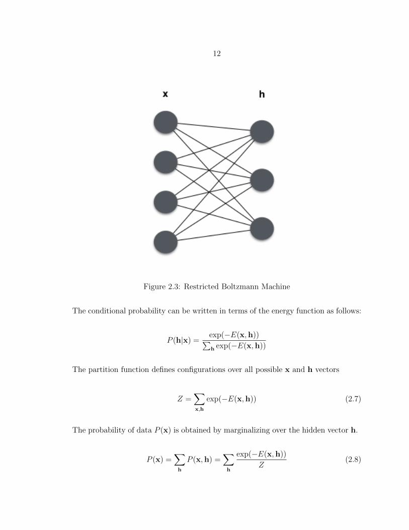
12
Figure 2.3: Restricted Boltzmann Machine
The conditional probability can be written in terms of the energy function as follows:
P (h|x) =exp(−E(x,h))∑h exp(−E(x,h))
The partition function defines configurations over all possible x and h vectors
Z =∑x,h
exp(−E(x,h)) (2.7)
The probability of data P (x) is obtained by marginalizing over the hidden vector h.
P (x) =∑h
P (x,h) =∑h
exp(−E(x,h))
Z(2.8)
13
The energy function of an RBM is then given as
E(x,h) = −h>Wx− b>x− c>h
Here, b and c are bias vectors on visible and hidden layers respectively.
We can rewrite the energy function as a sum over both hidden and visible nodes
as:
E(x,h) = −n∑j
m∑k
hjwjkxk −m∑k
bkxk −n∑j
cjhj
where n is number of hidden nodes and m number of visible (input) nodes. P (x)
defined in equation 2.8 can be written as the sum over all configurations of size n :
P (x) =∑
h∈0,1nexp(h>Wx + b>x + c>h)/Z
=∑
h1∈0,1
∑h2∈0,1
· · ·∑
hn∈0,1︸ ︷︷ ︸h∈0,1n
exp(h>Wx + b>x + c>h)/Z
=∑
h1∈0,1
∑h2∈0,1
· · ·∑
hn∈0,1
exp(n∑j=1
(hjwjx + b>x + cjhj)/Z
=∑
h1∈0,1
∑h2∈0,1
· · ·∑
hn∈0,1
n∏j=1
exp(hjwjx + b>x + cjhj)/Z
=n∏j=1
∑hj∈0,1
exp(hjwjx + b>x + cjhj)/Z
(2.9)
Since b>x is not dependent on h and it can be taken out of sum and product:
P (x) = exp(b>x)n∏j=1
∑hj∈0,1
exp(hjwjx + cjhj)/Z
14
Replacing h = 0 and h = 1, we obtain
P (x) = exp(b>x)n∏j=1
(1 + exp(wjx + cj))/Z
Using the fact exp(log(x)) = x, P (x) can be written as:
P (x) = exp(b>x +n∑j=1
log(1 + exp(wjx + cj)))/Z
Finally, f(x) = log(1+exp(x)) is the softplus function. Writing the above function
in term of softplus, we obtain the following equation:
P (x) = exp(b>x +n∑j=1
softplus(wjx + cj))/Z
Inspired from statistical mechanics, the exponential term F (x) = b>x+∑n
j=1 log(1+
exp(wjx + cj)) is called free energy. Thus,
P (x) = exp(−F (x))/Z (2.10)
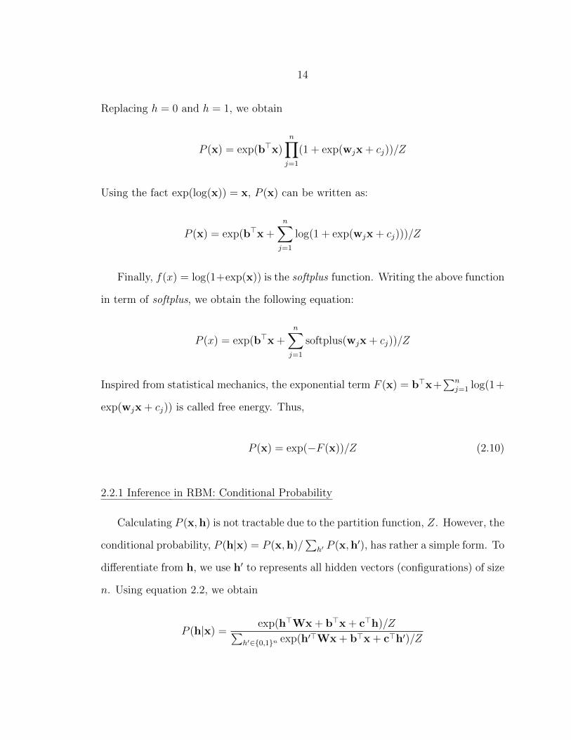
2.2.1 Inference in RBM: Conditional Probability
Calculating P (x,h) is not tractable due to the partition function, Z. However, the
conditional probability, P (h|x) = P (x,h)/∑
h′ P (x,h′), has rather a simple form. To
differentiate from h, we use h′ to represents all hidden vectors (configurations) of size
n. Using equation 2.2, we obtain
P (h|x) =exp(h>Wx + b>x + c>h)/Z∑
h′∈0,1n exp(h′>Wx + b>x + c>h′)/Z
15
The Z and b>x values cancel out. If we write this equation as an explicit sum over
all indices, we obtain
P (h|x) =exp(
∑nj=1 hjwjx + cjhj)∑
h′1∈0,1
∑h′2∈0,1
· · ·∑
h′n∈0,1︸ ︷︷ ︸h′∈0,1n
exp(∑n
j=1 h′jwjx + cjh′j)
Using c[∑t
n=s f(n)] =∏t
n=s cf(n) rule, we rewrite it as:
P (h|x) =
∏nj=1 exp(hjwjx + cjhj)∑
h′1∈0,1∑
h′2∈0,1· · ·∑
h′n∈0,1∏n
j=1 exp(h′jwjx + cjh′j)
Further we can rewrite the denominator as a product:
P (h|x) =
∏nj=1 exp(hjwjx + cjhj)∏n
j=1
∑h′j∈0,1
exp(h′jWjx + cjh′j)
The denominator can be simplified further using j = 0 and j = 1:
P (h|x) =
∏nj=1 exp(hjwjx + cjhj)∏nj=1(1 + exp(wjx + cj))
Using the same product, we obtain
P (h|x) =n∏j=1
exp(hjwjx + cjhj)
(1 + exp(wjx + cj))
It turns out that the term inside the product is a probability distribution. Thus,
it must be P (hj|x) because of the Markov property. As result, the equation can be
written as follows.
P (h|x) =n∏j=1
P (hj|x)
16
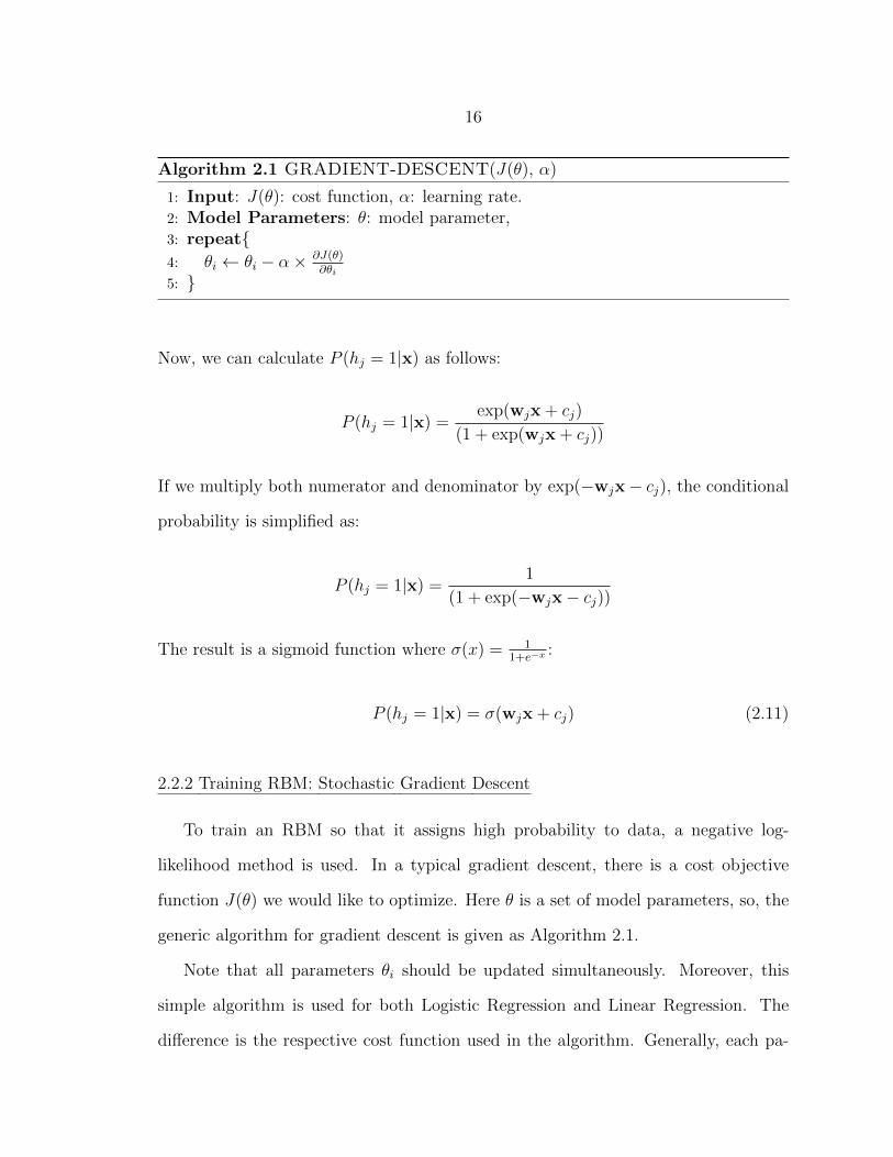
Algorithm 2.1 GRADIENT-DESCENT(J(θ), α)
1: Input: J(θ): cost function, α: learning rate.2: Model Parameters: θ: model parameter,3: repeat4: θi ← θi − α× ∂J(θ)
∂θi5:
Now, we can calculate P (hj = 1|x) as follows:
P (hj = 1|x) =exp(wjx + cj)
(1 + exp(wjx + cj))
If we multiply both numerator and denominator by exp(−wjx− cj), the conditional
probability is simplified as:
P (hj = 1|x) =1
(1 + exp(−wjx− cj))
The result is a sigmoid function where σ(x) = 11+e−x :
P (hj = 1|x) = σ(wjx + cj) (2.11)
2.2.2 Training RBM: Stochastic Gradient Descent
To train an RBM so that it assigns high probability to data, a negative log-
likelihood method is used. In a typical gradient descent, there is a cost objective
function J(θ) we would like to optimize. Here θ is a set of model parameters, so, the
generic algorithm for gradient descent is given as Algorithm 2.1.
Note that all parameters θi should be updated simultaneously. Moreover, this
simple algorithm is used for both Logistic Regression and Linear Regression. The
difference is the respective cost function used in the algorithm. Generally, each pa-
17
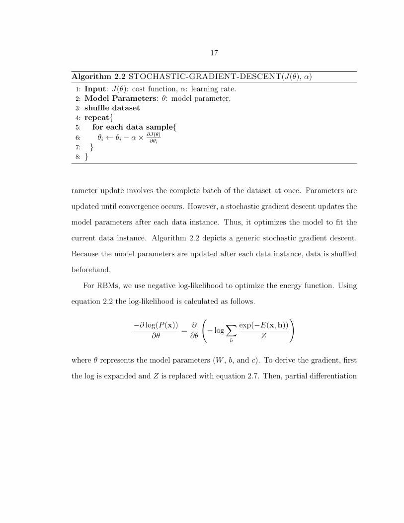
Algorithm 2.2 STOCHASTIC-GRADIENT-DESCENT(J(θ), α)
1: Input: J(θ): cost function, α: learning rate.2: Model Parameters: θ: model parameter,3: shuffle dataset4: repeat5: for each data sample6: θi ← θi − α× ∂J(θ)
∂θi7: 8:
rameter update involves the complete batch of the dataset at once. Parameters are
updated until convergence occurs. However, a stochastic gradient descent updates the
model parameters after each data instance. Thus, it optimizes the model to fit the
current data instance. Algorithm 2.2 depicts a generic stochastic gradient descent.
Because the model parameters are updated after each data instance, data is shuffled
beforehand.
For RBMs, we use negative log-likelihood to optimize the energy function. Using
equation 2.2 the log-likelihood is calculated as follows.
−∂ log(P (x))
∂θ=
∂
∂θ
(− log
∑h
exp(−E(x,h))
Z
)
where θ represents the model parameters (W , b, and c). To derive the gradient, first
the log is expanded and Z is replaced with equation 2.7. Then, partial differentiation
18
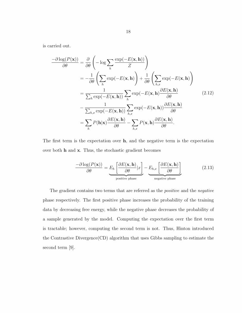
is carried out.
−∂ log(P (x))
∂θ=
∂
∂θ
(− log
∑h
exp(−E(x,h))
Z
)
= − 1
∂θ
(∑h
exp(−E(x,h)
)+
1
∂θ
(∑h,x
exp(−E(x,h)
)
=1∑
h exp(−E(x,h))
∑h
exp(−E(x,h)∂E(x,h)
∂θ
− 1∑h,x exp(−E(x,h))
∑h,x
exp(−E(x,h))∂E(x,h)
∂θ
=∑h
P (h|x)∂E(x,h)
∂θ−∑h,x
P (x,h)∂E(x,h)
∂θ.
(2.12)
The first term is the expectation over h, and the negative term is the expectation
over both h and x. Thus, the stochastic gradient becomes
−∂ log(P (x))
∂θ= Eh
[∂E(x,h)
∂θ|x]
︸ ︷︷ ︸positive phase
−Eh,x[∂E(x,h)
∂θ
]︸ ︷︷ ︸
negative phase
(2.13)
The gradient contains two terms that are referred as the positive and the negative
phase respectively. The first positive phase increases the probability of the training
data by decreasing free energy, while the negative phase decreases the probability of
a sample generated by the model. Computing the expectation over the first term
is tractable; however, computing the second term is not. Thus, Hinton introduced
the Contrastive Divergence(CD) algorithm that uses Gibbs sampling to estimate the
second term [9].
19
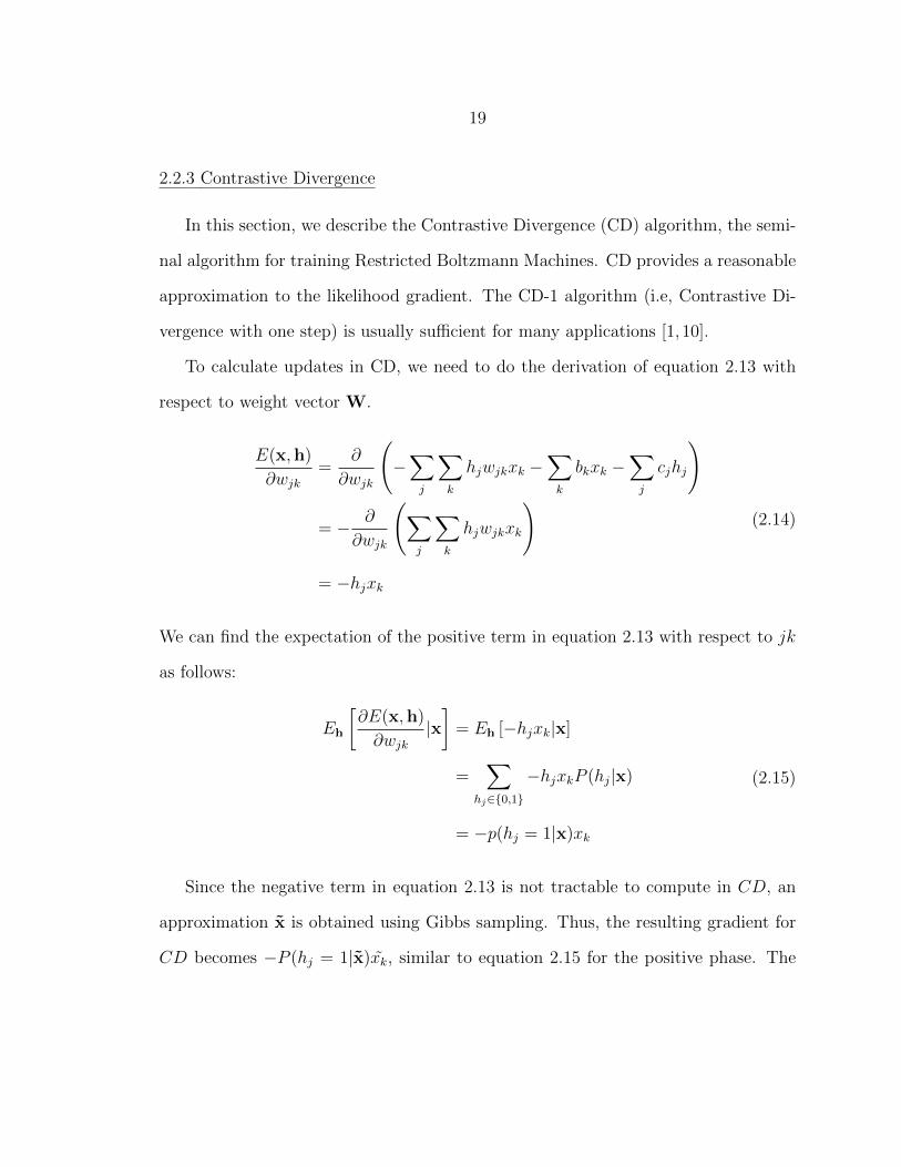
2.2.3 Contrastive Divergence
In this section, we describe the Contrastive Divergence (CD) algorithm, the semi-
nal algorithm for training Restricted Boltzmann Machines. CD provides a reasonable
approximation to the likelihood gradient. The CD-1 algorithm (i.e, Contrastive Di-
vergence with one step) is usually sufficient for many applications [1, 10].
To calculate updates in CD, we need to do the derivation of equation 2.13 with
respect to weight vector W.
E(x,h)
∂wjk=
∂
∂wjk
(−∑j
∑k
hjwjkxk −∑k
bkxk −∑j
cjhj
)
= − ∂
∂wjk
(∑j
∑k
hjwjkxk
)
= −hjxk
(2.14)
We can find the expectation of the positive term in equation 2.13 with respect to jk
as follows:
Eh
[∂E(x,h)
∂wjk|x]
= Eh [−hjxk|x]
=∑
hj∈0,1
−hjxkP (hj|x)
= −p(hj = 1|x)xk
(2.15)
Since the negative term in equation 2.13 is not tractable to compute in CD, an
approximation x is obtained using Gibbs sampling. Thus, the resulting gradient for
CD becomes −P (hj = 1|x)xk, similar to equation 2.15 for the positive phase. The
20
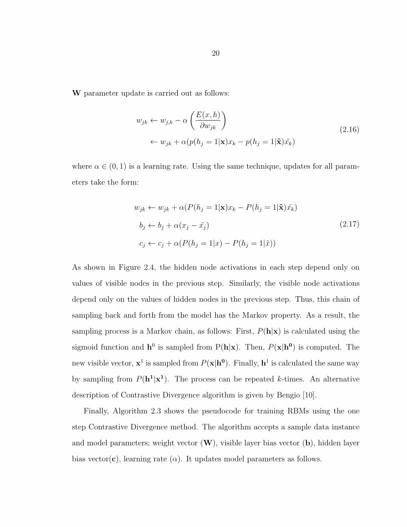
W parameter update is carried out as follows:
wjk ← wj,k − α(E(x, h)
∂wjk
)← wjk + α(p(hj = 1|x)xk − p(hj = 1|x)xk)
(2.16)
where α ∈ (0, 1) is a learning rate. Using the same technique, updates for all param-
eters take the form:
wjk ← wjk + α(P (hj = 1|x)xk − P (hj = 1|x)xk)
bj ← bj + α(xj − xj)
cj ← cj + α(P (hj = 1|x)− P (hj = 1|x))
(2.17)
As shown in Figure 2.4, the hidden node activations in each step depend only on
values of visible nodes in the previous step. Similarly, the visible node activations
depend only on the values of hidden nodes in the previous step. Thus, this chain of
sampling back and forth from the model has the Markov property. As a result, the
sampling process is a Markov chain, as follows: First, P (h|x) is calculated using the
sigmoid function and h0 is sampled from P(h|x). Then, P (x|h0) is computed. The
new visible vector, x1 is sampled from P (x|h0). Finally, h1 is calculated the same way
by sampling from P (h1|x1). The process can be repeated k-times. An alternative
description of Contrastive Divergence algorithm is given by Bengio [10].
Finally, Algorithm 2.3 shows the pseudocode for training RBMs using the one
step Contrastive Divergence method. The algorithm accepts a sample data instance
and model parameters; weight vector (W), visible layer bias vector (b), hidden layer
bias vector(c), learning rate (α). It updates model parameters as follows.
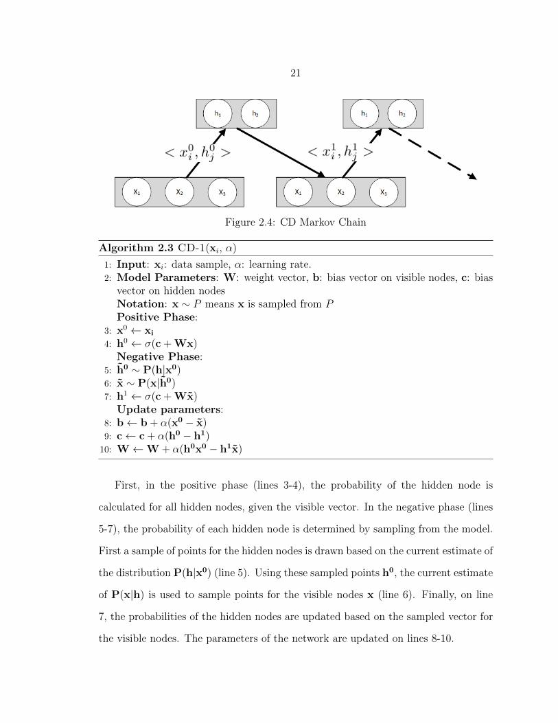
21
Figure 2.4: CD Markov Chain
Algorithm 2.3 CD-1(xi, α)
1: Input: xi: data sample, α: learning rate.2: Model Parameters: W: weight vector, b: bias vector on visible nodes, c: bias
vector on hidden nodesNotation: x ∼ P means x is sampled from PPositive Phase:
3: x0 ← xi
4: h0 ← σ(c + Wx)Negative Phase:
5: h0 ∼ P(h|x0)6: x ∼ P(x|h0)7: h1 ← σ(c + Wx)
Update parameters:8: b← b + α(x0 − x)9: c← c + α(h0 − h1)10: W←W + α(h0x0 − h1x)
First, in the positive phase (lines 3-4), the probability of the hidden node is
calculated for all hidden nodes, given the visible vector. In the negative phase (lines
5-7), the probability of each hidden node is determined by sampling from the model.
First a sample of points for the hidden nodes is drawn based on the current estimate of
the distribution P(h|x0) (line 5). Using these sampled points h0, the current estimate
of P(x|h) is used to sample points for the visible nodes x (line 6). Finally, on line
7, the probabilities of the hidden nodes are updated based on the sampled vector for
the visible nodes. The parameters of the network are updated on lines 8-10.
22
Contrastive Divergence need not be limited to one forward and backward pass in
this matter, and Algorithm 2.3 can be extended by creating a loop around lines 3–7.
Then for k > 1, the positive and negative phases are repeated k times before the
parameters are updated.
2.3 Autoencoders
An Autoencoder is a feed-forward neural net that predicts its own input [11].
It often introduces one or more hidden layers that have lower dimensionality than
the inputs so that it creates a more efficient code for the representation [3]. As
a generative model, the autoencoder encodes the input x into some representation
c(x); the input can be reconstructed from the resulting code.
Training is done by using reconstruction error. The training process involves
updating model parameters (weights and biases) by minimize this reconstruction
error [10].
Bengio claimed that if the autoencoder is trained with one linear hidden layer by
minimizing squared error, then the resulting code corresponds to principal compo-
nents of the data. However, if the hidden layer is non-linear, the autoencoder has a
different representation than PCA. It has the ability to capture multi-modal aspects
of the input distribution. Often, the following formula is used to minimize negative
log-likelihood of the reconstruction, given the encoding c(x):
reconstruction error = logP (x|c(x))
23
For binary x ∈ [0, 1]d, the the loss function can be written as:
logP (x|c(x)) =n∑i
xi log fi(c(x)) + (1− xi) log(1− fi(c(x)))
where n is number features and f(·) is the decoder. Thus, the network will generate
the input as f(c(x)). c(x) is a lossy compression. Both encoder and decoder functions
are sigmoid function:
y = c(x = σ(Wx + c)
where W is the weight matrix and c is the bias vector in the hidden nodes. The
decoder can be written as:
z = f(y) = σ(WTy + b)
where c is bias vector on input nodes and z is the reconstructed input vector.
2.4 Deep Learning
The performance of machine learning algorithms depends heavily on the set of
features used in the model. Thus, a feature detector is the first component of a
learning process. Using extracted features, the learning algorithm forms a hypothesis
that functions as a learned model. A feature is one or more attributes of the dataset
(or some transformation of the attributes) considered important in describing the
data. For example, in the handwritten digit recognition task, using raw pixel values
may not be sufficient. Many learning methods either rely on derived features such
as the gradient of histograms, while others project raw pixels onto a higher dimen-
sions. Feature engineering is an expansive process and often requires domain specific
24
knowledge. In an attempt to achieve a more generic algorithm, it is desirable that
the algorithm does not depend on this feature extraction process. In other words,
ideally the algorithm should identify the explanatory factors automatically.
According to Bengio et al. [4] a good representation, in the case of a probabilistic
model, is the one that captures the posterior distribution of the underlying explana-
tory factors for the observed input. Deep learning methods learn representations by
composition of multiple non-linear transformations in order to obtain more abstract
representations.
As stated by Bengio et al. [4] a good representation is expressive and distributive;
a reasonable representation can capture many possible input configurations. The
second most important aspect of representation is abstraction. Abstract concepts are
formed in terms of less abstract features and abstract concepts are generally invariant
to local changes of the input. Finally, the third aspect of good representation is that
it must disentangle the factors of variation. Because different explanatory factors of
the data tend to change independently in the input distribution, disentangling these
factors may lead to better representations.
In 2006, Hinton et al. experimented with a deep learning architecture [11] and
demonstrated that a network with multiple layers can represent features superior to
many traditional methods. Since then, deep learning has become one of the most
active research areas in machine learning. The core idea is to learn a hierarchy of
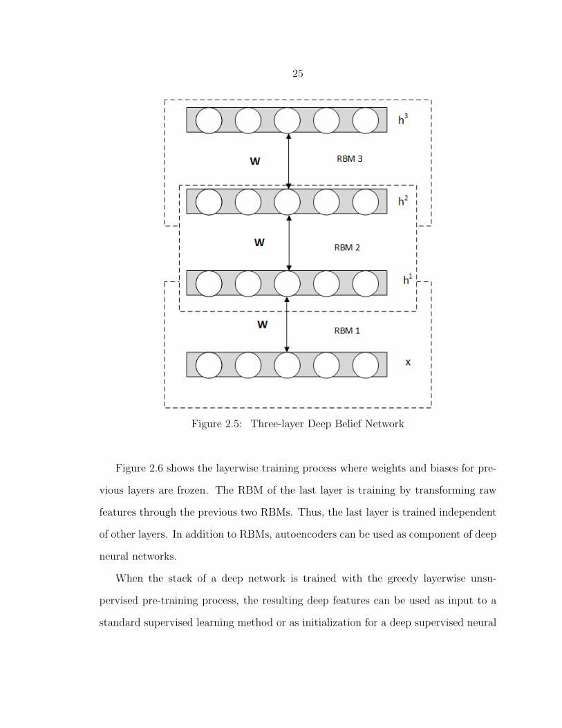
features one level at a time in an unsupervised fashion. Each level is composed with
previously learned transformations. Figure 2.5 illustrates a stack of RBMs where
input to each layer is the output of the previous layer. A typical learning process
involves unsupervised learning of one layer at a time in a greedy fashion. This learning
method is called “greedy layerwise unsupervised training.”
25
Figure 2.5: Three-layer Deep Belief Network
Figure 2.6 shows the layerwise training process where weights and biases for pre-
vious layers are frozen. The RBM of the last layer is training by transforming raw
features through the previous two RBMs. Thus, the last layer is trained independent
of other layers. In addition to RBMs, autoencoders can be used as component of deep
neural networks.
When the stack of a deep network is trained with the greedy layerwise unsu-
pervised pre-training process, the resulting deep features can be used as input to a
standard supervised learning method or as initialization for a deep supervised neural
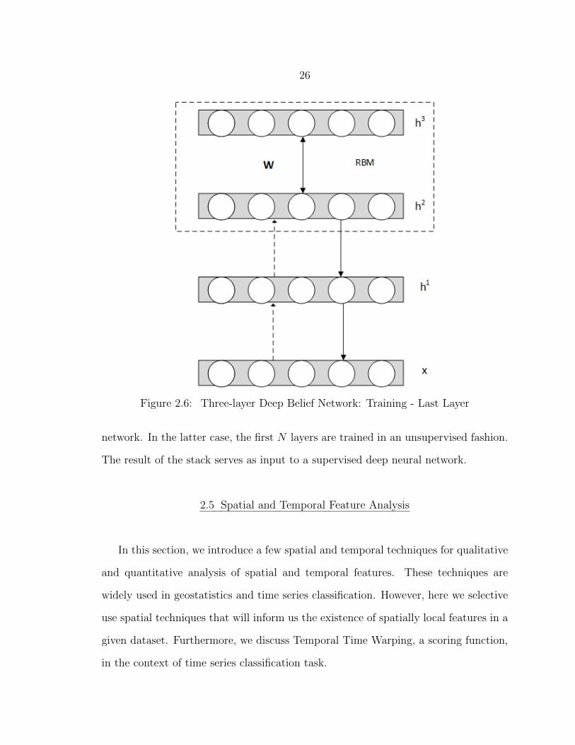
26
Figure 2.6: Three-layer Deep Belief Network: Training - Last Layer
network. In the latter case, the first N layers are trained in an unsupervised fashion.
The result of the stack serves as input to a supervised deep neural network.
2.5 Spatial and Temporal Feature Analysis
In this section, we introduce a few spatial and temporal techniques for qualitative
and quantitative analysis of spatial and temporal features. These techniques are
widely used in geostatistics and time series classification. However, here we selective
use spatial techniques that will inform us the existence of spatially local features in a
given dataset. Furthermore, we discuss Temporal Time Warping, a scoring function,
in the context of time series classification task.
27
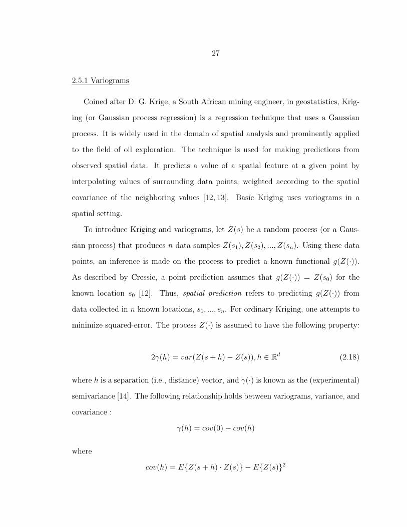
2.5.1 Variograms
Coined after D. G. Krige, a South African mining engineer, in geostatistics, Krig-
ing (or Gaussian process regression) is a regression technique that uses a Gaussian
process. It is widely used in the domain of spatial analysis and prominently applied
to the field of oil exploration. The technique is used for making predictions from
observed spatial data. It predicts a value of a spatial feature at a given point by
interpolating values of surrounding data points, weighted according to the spatial
covariance of the neighboring values [12, 13]. Basic Kriging uses variograms in a
spatial setting.
To introduce Kriging and variograms, let Z(s) be a random process (or a Gaus-
sian process) that produces n data samples Z(s1), Z(s2), ..., Z(sn). Using these data
points, an inference is made on the process to predict a known functional g(Z(·)).
As described by Cressie, a point prediction assumes that g(Z(·)) = Z(s0) for the
known location s0 [12]. Thus, spatial prediction refers to predicting g(Z(·)) from
data collected in n known locations, s1, ..., sn. For ordinary Kriging, one attempts to
minimize squared-error. The process Z(·) is assumed to have the following property:
2γ(h) = var(Z(s+ h)− Z(s)), h ∈ Rd (2.18)
where h is a separation (i.e., distance) vector, and γ(·) is known as the (experimental)
semivariance [14]. The following relationship holds between variograms, variance, and
covariance :
γ(h) = cov(0)− cov(h)
where
cov(h) = EZ(s+ h) · Z(s) − EZ(s)2
28
and
cov(0) = var(Z(s))
Semivariance measures differences in observed values over a set of distance bands or
lags. For such a function to be defined properly, some fairly strong assumptions about
the data must be made (including but not limited to it being sampled from a static,
isotropic spatial distribution).
In order to compute variograms, one has to find the squared differences between
all pairs of values in the dataset first. Then, these differences are allocated to lag
classes (bins) based on the distance separating the pair (often the direction is also
considered). The result is a set of semivariance values for distance lags, h = 0, ..., H
where H is less than the greatest distance between pairs. When plotting bin values
per lag, the resulting graph is called a variogram plot. In a way, the bins are inter-
feature (i.e. sampling location) distances, and the height of each column is the mean
of the variance of the (sample value) differences between all feature pairs that are
that distance apart. If we can model the inter-feature variance with distance using
a variogram, the values at unknown distances can be predicted or estimated by an
interpolation process.
2.5.2 Autocorrelation and Correlograms
In order to estimate linear predictors, the following assumption is also made:
cov(Z(s1), Z(s2)) = C(s1− s2),∀s1, s2
29
where C(·) is called covariogram or stationary covariance function [12]. This function
is called autocovariance function by time-series analysts. When C(0) > 0,
ρ(h) = C(h)/C(0) (2.19)
is called correlogram. In the time-series field, this measure is called autocorrelation.
Autocorrelation is used to diagnose non-stationarity in time series. Thus, if Z(·) is
stationary, then the following holds:
2γ(h) = 2(C(0)− C(h)) (2.20)
We can make a similar histogram using correlations (or any other pair-wise statisti-
cal measure) between feature-pairs of a given distance. A serial correlation coefficient
is given below for lag h:
ρ(h) =
n−h∑t=1
(xt − x)(xt+k − x)
n∑t=1
(xt − x)
(2.21)
For a random series, the ρ(h) values for all h time steps will be approximately
0. They will be distributed according to N(0, 1/n) [14]. If there is a short term
correlation, the ρ(h) will start at 1.0 and decrease gradually to 0 as the distances
increase. If the overall process shows a steady increase over time, the correlogram
will not be zero. This determines that the time series is not stationary.
In spatial statistics, the concept is adapted to spatial data, but it is not easy to
translate this directly to spatial statistics. Often, on a 2D grid, joint counts of events
30
are calculated and the probability of a particular pattern is estimated. This yields
formulas that are similar to the correlogram in time-series.
For a more in depth treatment of variograms, correlograms, and spatial statistics
in general, the reader is directed to books on the subject [12] and [14].
2.5.3 Distributed Stochastic Neighbor Embedding
To embed data in a 2-dimensional space for visualization, t-Distributed Stochastic
Neighbor Embedding (t-SNE) has been shown to be an effective technique [15]. More-
over, t-SNE is also a dimensionality reduction technique that is particularly good for
visualizing high dimensional data.
The t-SNE method is similar to Multidimensional Scaling (MDS) and Locally
Linear Embedding (LLE) techniques. MDS computes the low dimensional embedding
that preserves pairwise distances between data points [16]. On the other hand, LLE
builds a map of similarities in the data by finding a set of the nearest neighbors of
each point. It then computes a weight for each data point as a linear combination of
distances to its neighbor [17]. Both MDS and LLE use eigenvector-based optimization
techniques to find the low-dimenstional embedding of the points.
The t-SNE method builds a map in which distances between points reflect sim-
ilarities in the data. It embeds high-dimensional data in lower dimensional space
by minimizing the discrepancy between pairwise statistical relationships in the high
and low dimensional spaces. For a dataset of n points, let i, j ∈ [1, n] be indices,
and let xi ∈ X and yi ∈ Y refer to the ith datapoint of the original dataset and
the low-dimensional equivalent respectively. Given a candidate embedding, t-SNE
first calculates all pairwise Euclidean distances between data points in each space.
The pairwise Euclidean distance between xi and xj is used to calculate a conditional
31
probability, Pj|i, which is the probability that xi would pick xj as its neighbor. This
probability is based on a Gaussian centered at xi. Similarly, pairwise conditional
probabilities qj|i are calculated for each pair (yi, yj) in the low-dimensional embed-
ding. As an objective function, t-SNE tries to minimize the discrepancies between
the conditional probabilities for corresponding pairs in the high dimensional and low
dimensional spaces by using Kullback-Leibler divergence (KL-divergence). This is an
intractable global optimization problem, so often gradient descent is used to find a
local optimum.
One drawback of t-SNE is that for large, high-dimensional datasets, even the local
search can be quite slow. In such cases, PCA is sometimes used as a pre-processing
step to speed up the computation and to suppress high-frequency noise. A typical
example might retain the top 30 eigenvectors and project the original data into the
eigenbasis. t-SNE would then be applied to this 30-dimensional dataset to reduce it
to a 2-dimensional set for visualization.
The resulting 2D plots make the structure (or lack thereof) readily apparent.
Since the optimization is done on pair-wise vector distances, feature ordering (i.e.
spatially local structure) in the high-dimensional data does not change the qualitative
properties of the low-dimensional data significantly. Moreover, since the mapping is
non-linear and non-parametric, it is relatively insensitive to whether information is
encoded using sparse or distributed representations. As a result, t-SNE allows us
to examine the presence of structure without having to worry about the form of
that structure impacting our analysis. Figure 2.7 shows a 2D embedding of MNIST
dataset using t-SNE.
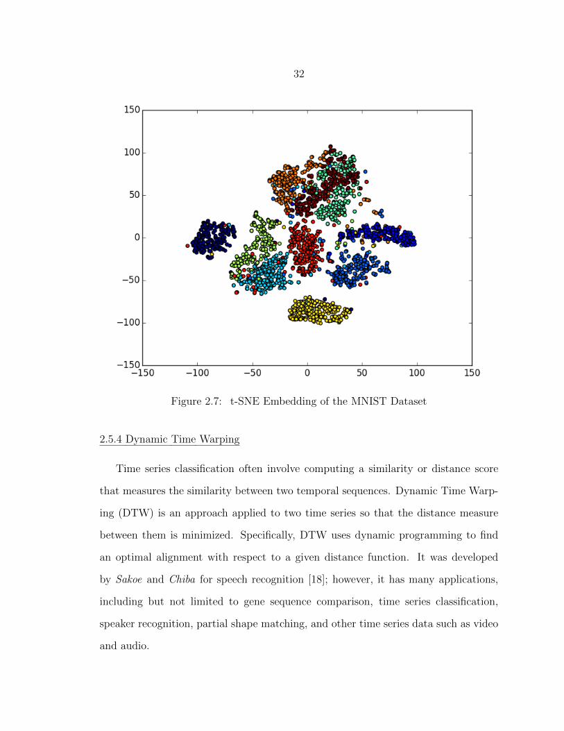
32
Figure 2.7: t-SNE Embedding of the MNIST Dataset
2.5.4 Dynamic Time Warping
Time series classification often involve computing a similarity or distance score
that measures the similarity between two temporal sequences. Dynamic Time Warp-
ing (DTW) is an approach applied to two time series so that the distance measure
between them is minimized. Specifically, DTW uses dynamic programming to find
an optimal alignment with respect to a given distance function. It was developed
by Sakoe and Chiba for speech recognition [18]; however, it has many applications,
including but not limited to gene sequence comparison, time series classification,
speaker recognition, partial shape matching, and other time series data such as video
and audio.
33
Consider two time series s and t with length n and m respectively. The key idea
in DTW is that sequences s and t can be arranged to form a n×m grid where each
point (i, j) is the alignment between element si and tj. The warping path, W , is
constructed to align elements of s and t such that it minimizes the distance between
them. Since W forms a sequence of grid points (W = w1, w2, . . . wk), each w value
corresponds to a grid point (i, j) .
The warping path is subject to the following constraints:
• Boundary conditions: the warping path starts at (0, 0) and ends at (n,m).
• Continuity: the warping path only traces adjacent points in the grid.
• Monotonicity: the points must be ordered monotonically with respect to time.
Thus, the DTW is a minimization over potential warping paths. Although there are
an exponential number of paths, we calculate the minimum-cost path using dynamic
programming as follows:
γ(i, j) = δ(i, j) + minγ(i− 1, j), γ(i− 1, j − 1), γ(i, j − 1) (2.22)
where γ(i, j) is the cumulative distance and δ(i, j) is the cost function between two
points.
Several distance functions can be used. Following are the two most common
distance functions:
δ(i, j) = ‖si − ti‖
δ(i, j) = ‖si − ti‖2(2.23)
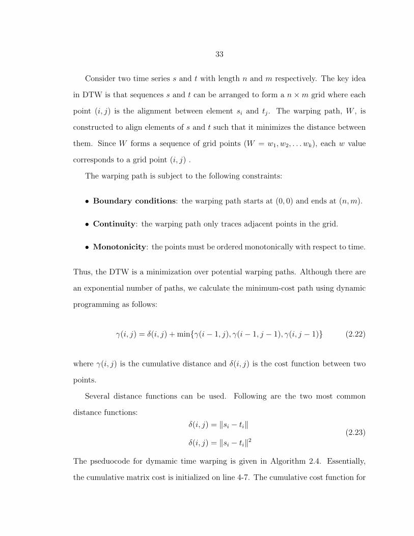
The pseduocode for dymamic time warping is given in Algorithm 2.4. Essentially,
the cumulative matrix cost is initialized on line 4-7. The cumulative cost function for

34
Algorithm 2.4 DTW(s, t)
1: s: time series 1, t: time series 22: n← s.size3: m← t.size4: γ: matrix of size s and t5: γ[: 0]←∞6: γ[0 :]←∞7: γ[0 : 0]← 08: for i← 1 until n 9: for j ← 1 until m 10: cost = δ(si, tj)11: γ(i, j) = cost+ minγ(i− 1, j), γ(i− 1, j − 1), γ(i, j − 1)12: 13: 14: return γ(n,m)
each point is calculated on line 11. Since this algorithm iterate over both time series,
the time complexity of the algorithm is O(n2).
35
CHAPTER 3
RELATED WORK
In this chapter we present a review of literature related to sampling methods,
Restricted Boltzmann Machines, deep learning, autoencoders, spatial statistics and
time series classification.
3.1 Sampling Methods
Welling and Teh introduced a Bayesian learning method based on Stochastic Gra-
dient Langevian dynamics (SGLD) [19]. They claim that in order for Bayesian meth-
ods to be practical in large scale machine learning, stochastic methods need to be
adapted because a typical Markov Chain Monte Carlo (MCMC) algorithm requires
computations over the whole dataset. Thus, the authors proposed a method that
combines Robbins-Monro type algorithms that stochastically optimize a likelihood
function with Langevin dynamics. Langevin dynamics is stochastic graident that
inject a noise into the parameter update so that the trajectory of the parameters will
converge to the full posterior distribution rather than just the maximum a posterior
mode. In order to sample from the posterior, the authors introduced a mini-batch
technique where parameters are updated after a single mini-batch. In other words, the
stochastic gradient is a sum over the current mini-batch of size n. Thus, this algorithm
requires O(n) computations to generate one sample. Unlike the long burn-in time that
MCMC uses, this technique enable one to use a large dataset. They discovered that if
the injected noise is distributed normally with an ε variance N(0, εt) where et changes
per iteration, the dynamics becomes Langevin. Welling and Teh observed that the
36
stochastic gradient noise dominates initially, and the algorithm behaves as an efficient
stochastic ascent algorithm. However, for large t, as ε → 0, the injected noise will
dominate the stochastic gradient and the MH rejection probability will approach 0.
Key findings of this research are, 1) SGLD can generate samples from a posterior
at O(n) complexity where n N , and 2) under certain conditions, the posterior
can be approximated by a normal distribution. However, one disadvantage of this
method is that, with an increasing number of iterations, the mixing rate of algorithm
decreases. To address this issue, they proposed to keep the step size to a constant
once it has decreased to a critical threshold. Nonetheless, SGLD takes large steps in
the direction of small variance and smalls steps in directions of large variance. This
results in the slow mixing rate.
Anh and Welling followed the same line research to address the slow mixing rate
using Fisher Scoring [20]. The question asked was “Can we approximately sample
from a Bayesian posterior distribution if we are only allowed to touch a small mini-
batch of data-items for every sample we generate?” Based on Bayesian asymptotic
theory, as N becomes large, the posterior distribution becomes Gaussian. This is
called the Bayesian Central Limit Theorem [21]. The theorem states that, under
certain regularity conditions, p(θ|x1, ..., xN) ' N(θ0, I−1N ) where IN is the Fisher in-
formation. Moreover, the Fisher information is the average covariance of gradients
calculated from a mini-batch. Thus, the authors replaced Langevin dynamics with
Fisher information. Unlike SGLD, this method was designed such that it samples
from a Gaussian approximation of the posterior distribution for large step sizes, thus,
increasing the mixing rate. Perhaps the most importing aspect of the above is tradein
a small bias in the estimate of posterior against computational gains: this method
allows us to use more samples and as a result, it reduces sampling variance. In our
37
partitioned method, we apply the same concept; more partitioning allows us to use
more samples, which in turn results in more accurate generative models.
3.2 Restricted Boltzmann Machines
After first proposed by Smolensky [7] in 1986, the Restricted Boltzmann Ma-
chine did not gain popularity for almost 17 years. Although training of the RBM
was tractable, it was initially inefficient. Slow computers and the limiation to using
small datasets also contributed the slow adoption of RBMs. With better compu-
tational resources and bigger datasets, and Hinton’s et al. development of Con-
trastive Divergence [9], RBMs are now used as basic components of deep learning
algorithms [11, 22, 23] and successfully applied to classification tasks [24–26]. More-
over, RBMs have been applied to many other learning tasks including Collaborative
Filtering [27].
As RBMs became popular, research on training them efficiently increased. Gibbs
sampling is a Markov chain Monte Carlo (MCMC) sampling algorithm [28] for obtain-
ing a sequence of samples from a posterior distribution. It is an iterative process that
samples from a distribution closer to the posterior distribution. The graph of states
over which the sampling algorithm produces samples is called a “Markov Chain.”
As we described in the Section 2.2.3, the Contrastive Divergence algorithm performs
Gibbs sampling for k-steps to compute weight updates. However, for each data sam-
ple, it creates a new Markov Chain. In other words, the state of the Markov chain is
not preserved for subsequent updates. Tieleman modified the Contrastive Divergence
method by making Markov chains persistent [1]. In other words, the Markov chain is
not reset for each training example. This has been shown to outperform Contrastive
Divergence with one step, CD-1, with respect to classification accuracy. Even so,
38
many applications have demonstrated minimal (if any) improvement in performance
using persistent Markov chains. Brekal et al. introduced an algorithm to parallelize
training RBMs using parallel Markov chains [29]. They run several Markov chains in
parallel and treat this set of chains as a composite chain; the gradient is approximated
by weighted averages of samples from all chains.
When RBMs are trained in an unsupervised fashion, there is no guarantee that
the hidden layer representing learned features will be useful for a classification task.
Thus, there is considerable research on RBMs in supervised or semi-supervised learn-
ing when labeled data is available [24–26,30–32]. One of the most significant current
research achievements with RBMs by Larochelle et al. is to apply them as a stan-
dalone classifier [25]. In combination with a generative objective function, Larochelle
et al. developed a discriminative objective function to train RBMs as classifiers. It
was demonstrated that when a hybrid objective function is used, the classification
accuracy can be increased significantly. Interestingly, as demonstrated and discussed
in detail in Chapter 5, the results could not be replicated due to an overflow when
computing the gradient of the discriminative objective function.
Schmah et al. took a different approach in applying RBMs to classification tasks:
instead of using a monolithic RBM to represent all classes, the authors trained one
RBM per class label [33]. However, a major drawback of this approach is that it
cannot model latent similarities between classes. Nonetheless, an interesting result of
their study is the demonstration that generative training can improve discriminative
performance, even if all data are labeled. Studying two methods of training, one
almost entirely generative and one discriminative, the authors found that a genera-
tively trained RBM yielded better discriminative performance for one of the two tasks
studied.
39
3.3 Deep Learning
As described in Section 2.4, according to Bengio et al., good representation is the
basis for deep learning [4]. Deep learning develops good representation by composi-
tions of multiple non-linear transformations in order to obtain more abstract represen-
tations. Bengio et al. gives most important aspects of good representations: 1) They
must be expressive and distributive. That is, a reasonable representation should cap-
ture many possible input configurations. 2) They must be abstract representations.
Since abstract concepts are formed in terms of lower level features, abstract concepts
must be invariant to the input. 3) They must disentangle the factors of variation. For
instance, images of faces may contain factors of variation such as pose (translation,
scaling, rotation), identity (male, female), and other attributes. Disentangling these
factors results in finding abstract features that minimize dependence and are more
invariant to most of these variations.
There were other attempts to derive a theory to explain the success of deep
learning. Erhan and Bengio [34] suggest that unsupervised pre-training acts as a
regularizer, and we have suggested in previous work [35] that it also takes advantage
of spatially local statistical information in the training data.
Historically, deep networks were difficult to train because of a credit assignment
problem; standard error-backpropagation suffers from gradient diffusion if applied to
a deep network, resulting in generally poor performance [36]. Most deep learning
techniques now get around this problem by performing some form of “unsupervised
pre-training,” which often involves learning the weights to minimize reconstruction
error for (unlabeled) training data, one layer at a time in a bottom up fashion. This is
40
then followed by a supervised learning algorithm that, it is hoped, has been initialized
in a good part of the search space.
When Restricted Boltzmann Machines are used to form a DBN, the network is
trained layer-wise while minimizing reconstruction error. This is a form of unsu-
pervised pre-training. Once all layers have been trained, the resultant network can
then be used in different ways, including adding a new output layer and running a
standard gradient descent algorithm to learn a supervised task such as classification.
The aim of stacking RBMs in this way is to learn features in order to obtain a high
level representation.
While techniques similar to modern deep learning algorithms have been proposed
previously (see Fukushima [37], for example), it has only been the past few years that
have seen deep learning come into its own. Hinton et al. were the first to experiment
with deep learning architectures after developing an efficient algorithm for training
RBMs [38]. Their results suggested that networks with multiple layers can represent
features that are distributive and abstract.
Following this seminal discovery, deep learning has become one of the most active
research areas. Several studies on deep learning were quickly published following
Hinton’s discovery in 2006: In the same year, Ranzato et al. developed a deep sparse
encoder [39]. In 2007, Bengio et al. explored variants of DBN and extended it to
continuous input values [22]. Two years later, Lee et al. developed a sparse variant of
the deep belief network [40]. The core idea in these early studies is to learn a hierarchy
of features one level at a time and in unsupervised fashion. A typical learning involves
unsupervised learning of one layer at a time in greedy fashion.
Typically, autoencoders and RBMs are used as components for deep learning
[10, 11, 22, 23, 41, 42]. In other words, RBMs and autoencoders are used to form a
41
deep neural network model. It was shown that layerwise stacking of RBMs and auto
encoders yielded better representation [43,44].
With large initial weights, Hinton and Salakhutdinov discovered that autoencoders
typically find poor local minima [11]. On the other hand, with small initial weights,
the gradients in the early layers are tiny, thus, making it infeasible to train autoen-
coders with many hidden layers. Hinton and Salakhutdinov describe a method for
effectively initializing the weights that allows deep autoencoder networks to learn low-
dimensional codes. This is accomplished by pretraining on a stack of RBMs. After
pretraining, the RBMs “unrolled” to create a deep autoencoder. The autoencoder
is then fine-tuned using backpropagation of the error derivatives. It is also possible
that an autoencoder with more hidden nodes than visible/input nodes to learn the
identity [10]. It was shown by Ranzato et al. that when sparsity is introduced in
hidden layers, autoencoders creates more efficient representations [39]. These types
of autoencoders are known as sparse autoencoders.
To make learned representations of autoencoders robust to partial corruption of
the input pattern, Vincent et al. explicitly introduced partial corruption of the input
that is fed to the network [45]. The stochastic corruption process randomly cor-
rupts some inputs to be 0. Hence, the denoising autoencoder is trying to predict the
corrupted (i.e. missing) values from the uncorrupted (i.e., non-missing) values for ran-
domly selected subsets of missing patterns. These denoising autoencoders are shown
have better learned representations [45]. Denoising autoencoders can be defined in
terms of information theory, and Vincent theorized that minimizing the expected
reconstruction error amounts to maximizing a lower bound on mutual information.
Xie et al. argue that training denoising autoencoders with noise patterns that fit to
specific situations can also improve the performance of unsupervised feature learning
[46].
42
Convolutional Neural Networks (CNN), developed by LeCun [47,48] are also con-
sidered as deep architectures. CNNs exploit spatially-local features by combining
neurons of adjacent layers. In other words, the input of a hidden unit may come from
a subset of units in the previous layer. Moreover, in CNNs, each hidden node filter is
replicated across the entire visual fields. The replicated units share the same weight
and bias vectors. This enables the model to detect features regardless their position.
CNNs demonstrated good performance for a number of traditionally difficult tasks,
many in the domain of computer vision. Some examples are handwritten character
recognition and object recognition.
Similar to Convolutional Neural Networks, Lee et al. developed a Convolutional
Deep Belief Network (CDBN) model composed of redundant RBMs where each RBM
has V × V visible nodes and K group of H × H binary hidden units [49]. V × V
represents the image dimensions. Each group K is associated with a set of shared
weights. In addition to a hidden layer (detection layer), the network also has a pooling
layer of K groups of units with P × P binary units each. The authors demonstrated
that a DBN based on this model is translation-invariant, and it efficiently learns
hierarchical representations from unlabeled images. These findings are consistent
with other studies on Convolutional Neural Networks.
The Deep Boltzmann Machine (DBM) is another type of deep learning architec-
ture [43]. Like DBNs, the pretraining for DBMs is also greedy layer-wise, but in
DBMs, the training process involves creating two redundant RBMs (doubling the
inputs and doubling the hidden variables) and then using these two modules in esti-
mating the probabilities themselves. When these two modules are composed to form
a single network, the influence of the various nodes are halved. Salakhutdinov et
al. demonstrated that deep Boltzmann machines learn good generative models and
perform well on visual object recognition tasks.
43
3.4 Dropout
Dropout is a method to prevent neural networks from overfitting and improving
the performance of neural networks by preventing co-adaptation of feature detectors
by injecting noise in a model. A learning model with a large number of parameters
(e.g., neural networks) can easily overfit the training data. Thus, when a learning
model is trained on a small dataset, it naturally performs poorly on testing data
in that it can overfit the training data. When training a large feedforward neural
network, Hinton et al. introduced a dropout process, where for each training case
each hidden node is randomly omitted from the network with a probability [50]. This
technique assures that a hidden unit cannot rely on other hidden units being present.
Hinton et al. argued that the overfitting is greatly reduced by randomly omitting half
of the feature detectors in a feedforward neural networks.
Applying the same dropout concept to deep neural networks, Dahl et al., carried
out dropout in all hidden layers during supervised training [51]. When calculating
hidden node activations, the authors multiplied the net input from the layer below by
a factor of 11−r , where r is the dropout probability for units in the layer below. This
deep neural network with dropout performed well on a large speech recognition task.
In the same line of research, Srivastava et al. developed a dropout Restricted
Boltzmann Machine model and compare it to standard Restricted Boltzmann Ma-
chines. Applying to many speech, vision and text datasets, the authors demonstrated
that the dropout RBMs are better than standard RBMs [52]. However, the authors
noted that a large dropout rate may slow down training.
44
3.5 Partitioned Model Learning
While many learning techniques (such as Deep Belief Networks) treat all the
elements of an input vector as whole, some take an approach that partitions the
data vectors into shorter sub-vectors, and performs analysis on the sub-vectors before
re-combining the analyzed data to form a representation of the full data vector. Con-
volutional Networks are the most well known of these, though there are several others,
including [37,53] and [54]. Fukushima developed one of the earliest deep architecture
which he calls Self-organizing Neural Network Model [37]. The architecture strongly
resembles Convolutional networks. With the same line of research, Behnke and Rojas
proposed a hierarchical neural architecture with goal of transforming a given image
into a sequence of representation with increasing level of abstraction [53].
In the context of Deep Belief Networks (DBN), the DistBelief model and data
parallelization framework was developed by Dean et al. [55]. Here, the DBN model
is partitioned into parts. The overlapping parts then exchange messages. Moreover,
models are replicated in different computation nodes and trained on different subsets
of data to provide data parallelization. Although this algorithm is related to our
work, it is primarily a distributed stochastic gradient descent algorithm. In contrast
to this method, we partition a single RBM into multiple small RBMs and combine
the small RBMs to learn the final model.
Work by Schulz et al. is perhaps the first attempt to exploit partitioning in
RBM [56]. The authors observed that the connectivity of RBM is problematic when
they monitored learned features. Specifically, they observed that, typically, RBMs
learned localized features. They observed that in early stages, feature detectors are
global (represent global features). However, most of the detectors had uniform weights
45
as a result of very late stages of the learning process. Thus, the most training is
wasted. Similar to Dean et al. described above, they partition the network in fixed
regions. Unlike Dean et al., they also add lateral connections in the hidden layer
(connections between hidden nodes) to improve representational power of the model.
In short, Schulz et al. try to reduce the number of parameters to make learning
feasible at cost of relationships between long-range features. Although they attempt
partially to compensate for the effect of not modeling long-range interactions with
lateral connections, this method is not well-suited for data where long-range features
(e.g., relative configurations of an object in an image) are correlated significantly.
In promising research done by Strasser et al., Factored Evolutionary Algorithms
(FEA) are related to our partitioned training method [57]. Perhaps the most im-
portant aspect of this research is that they convert problems into Factor Graphs
and utilize stochastic or evolutionary algorithms to optimizes a set of parameters by
overlapping partitioned subpopulations. Each subpopulation optimizes a subset of
parameters. In addition to a subpopulation optimizing over a subset of parameters,
the authors defined a competition technique where the algorithm finds the subpop-
ulations with state assignments that have the best fitness for each dimension. In
order for overlapping subpopulations to share their current knowledge, the authors
defined a sharing method. Similarly, an RBM in its pure form can be regarded as a
Factor Graph; for a given visible vector, a hidden node is independent of other hid-
den nodes. Thus, each hidden node connecting to the visible nodes is a factor. One
can think of the each partition in our Partitioned-RBM as a factor Graph. Similar to
FEA, Partitioned-RBM optimizes only a subset of parameters using small partitioned
RBMs. However, our sharing algorithm is implicit. As we create fewer partitions, we
optimize over overlapping set of parameters; therefore, there is no need for an explicit
sharing technique.
46
3.6 Temporal Classification
DTW was first developed by Sakoe and Chiba for speech recognition [18]. In
addition, Sankof demonstrated that DTW can be applied to gene sequence comparison
[58]. In gene sequencing, for given finite sequences s and t, one needs to determine
the minimum number of substitutions, insertions, and deletions required to change s
into t.
Later, Bemdt and Clifford applied DTW to time series analysis for applications
in knowledge discovery [59]. The authors demonstrated that DTW can be used as
an efficient tool for discovering patterns in large time series datasets. Moreover, the
authors proposed that DTW can be used for both categorical and continuous data
by adding a temporal dimension (creating time series data).
In recent years, indexing large time series became an important task. Euclidean
distance was used in algorithms (e.g., k-Nearest Neighbor) to index the time series
data. Keogh and Ratanamahatana discovered that DTW is a more robust measure
for indexing time series [60]. It was proven that an indexing method based on DTW
not only guarantees no false dismissals, it can also index large datasets efficiently.
Ding et al. carried out a comprehensive study to compare various distance mea-
sures in querying and mining time series data [61]. Considering two key aspects of
time series data—representation methods and similarity measures—they compared
all measures for effectiveness and efficiency. Using 1-Nearest Neighbor (1-NN), the
authors experimented with various comparison measures including DTW and Eu-
clidean distance. Moreover, they demonstrated that for time series classification, as
the size of the training set increases, the accuracy of various measures converge to that
47
of Euclidean distance. But on small data sets, DTW is significantly more accurate
than Euclidean distance.
Following the same experiments carried out by Ding et al. described above, Wang
et al. also experimented with various methods for querying and mining time series
data [62]. In order to provide a comprehensive evaluation, they performed the exper-
iments on 38 time series data sets, from the UCR Time Series repository [63]. Their
findings on time series classification were also consistent with that of Ding.
Hu et al., developed a method for classifying of time series; however, they were
only concerned with the task of correctly extracting individual subsequences, such as
gait cycles, heartbeats, gestures, and behaviors. Since classification of a subsequence
is generally much more difficult than the task of actually classifying the whole time
series, they introduced an alignment-free algorithm for classification where it does
not require sequences to be closely related and be aligned perfectly. They maintained
that DTW does not work in subsequence classificaiton task [64].
Contradicting Hu et al., Rakthanmanon et al. maintained that DTW is the best
measure when applied to searching and mining trillions of time series subsequences.
They emphasized that normalizing subsequences helps classification accuracy of k-
NN [65]. In some real datasets, such as in a video sequence, features can be at
different scale and/or different offset. Algorithms that are not invariant to such
changes (e.g., k-NN) perform poorly, because small changes in some features can
have a dominating contribution to the distance function. The authors demonstrated
that k-NN had significantly higher classification accuracy on Z-normalized data as
compared with un-normalized data.
48
CHAPTER 4
PARTITIONED LEARNING
In this chapter, we first develop a generic learning method via partitioning the
model into sub components. Each component is in turn trained on a subsection of the
input vector. This training process is the main contribution of this work. We then
apply this technique to Restricted Boltzmann Machines (RBMs). In the remaining
chapters, we demonstrate that this method not only improves runtime complexity of
training algorithms, it also significantly improves performance of the learning methods
in terms of classification accuracy and representation power.
4.1 Data Partitioning Theory
In order to train a partitioned model, we first need to describe how we partition
the input vectors. There are many ways to partition the data; however, any particular
partitioning method may have statistical effects on the learning model. Mitchell et
al. introduced the following notation to describe different partitioning schemes [66].
Given data vectors in Rn, we define a partitioning function π as
π : Rn → u0, . . . ,uk ,ui ∈ Rs,
which takes a single input vector in Rn and produces a set of k output vectors in Rs,
where s < n. This partitioning scheme creates subsets that can be either disjoint or
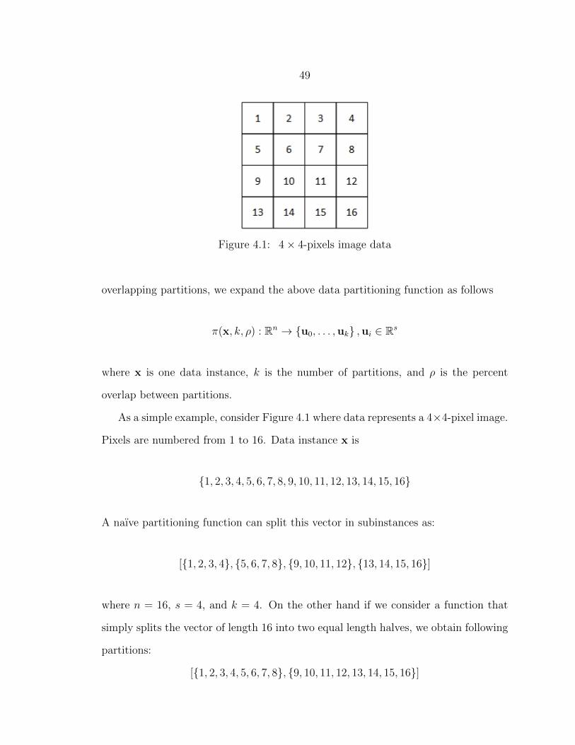
49
Figure 4.1: 4× 4-pixels image data
overlapping partitions, we expand the above data partitioning function as follows
π(x, k, ρ) : Rn → u0, . . . ,uk ,ui ∈ Rs
where x is one data instance, k is the number of partitions, and ρ is the percent
overlap between partitions.
As a simple example, consider Figure 4.1 where data represents a 4×4-pixel image.
Pixels are numbered from 1 to 16. Data instance x is
1, 2, 3, 4, 5, 6, 7, 8, 9, 10, 11, 12, 13, 14, 15, 16
A naıve partitioning function can split this vector in subinstances as:
[1, 2, 3, 4, 5, 6, 7, 8, 9, 10, 11, 12, 13, 14, 15, 16]
where n = 16, s = 4, and k = 4. On the other hand if we consider a function that
simply splits the vector of length 16 into two equal length halves, we obtain following
partitions:
[1, 2, 3, 4, 5, 6, 7, 8, 9, 10, 11, 12, 13, 14, 15, 16]
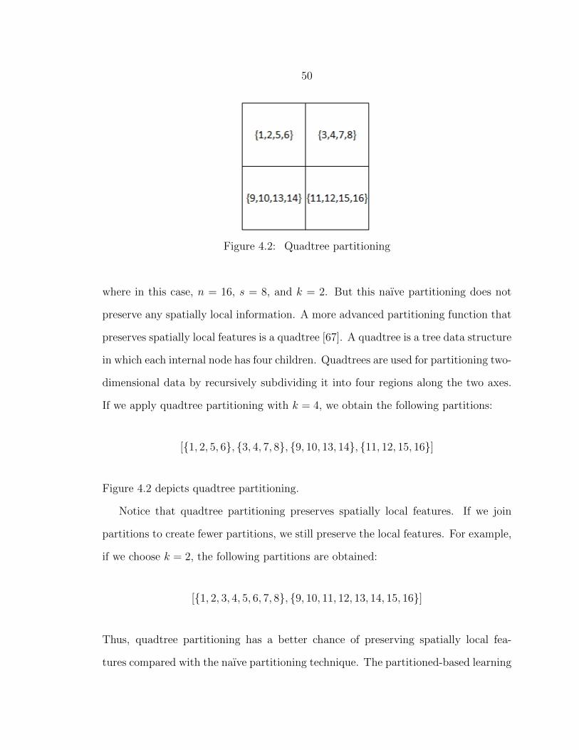
50
Figure 4.2: Quadtree partitioning
where in this case, n = 16, s = 8, and k = 2. But this naıve partitioning does not
preserve any spatially local information. A more advanced partitioning function that
preserves spatially local features is a quadtree [67]. A quadtree is a tree data structure
in which each internal node has four children. Quadtrees are used for partitioning two-
dimensional data by recursively subdividing it into four regions along the two axes.
If we apply quadtree partitioning with k = 4, we obtain the following partitions:
[1, 2, 5, 6, 3, 4, 7, 8, 9, 10, 13, 14, 11, 12, 15, 16]
Figure 4.2 depicts quadtree partitioning.
Notice that quadtree partitioning preserves spatially local features. If we join
partitions to create fewer partitions, we still preserve the local features. For example,
if we choose k = 2, the following partitions are obtained:
[1, 2, 3, 4, 5, 6, 7, 8, 9, 10, 11, 12, 13, 14, 15, 16]
Thus, quadtree partitioning has a better chance of preserving spatially local fea-
tures compared with the naıve partitioning technique. The partitioned-based learning
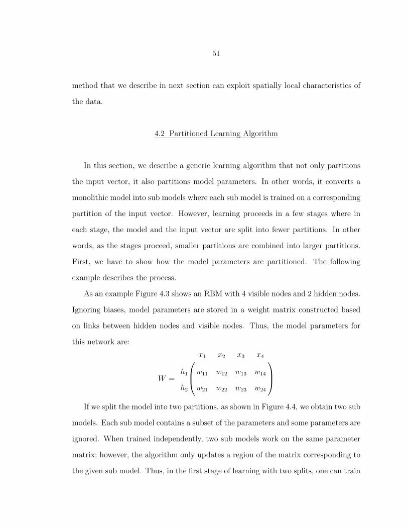
51
method that we describe in next section can exploit spatially local characteristics of
the data.
4.2 Partitioned Learning Algorithm
In this section, we describe a generic learning algorithm that not only partitions
the input vector, it also partitions model parameters. In other words, it converts a
monolithic model into sub models where each sub model is trained on a corresponding
partition of the input vector. However, learning proceeds in a few stages where in
each stage, the model and the input vector are split into fewer partitions. In other
words, as the stages proceed, smaller partitions are combined into larger partitions.
First, we have to show how the model parameters are partitioned. The following
example describes the process.
As an example Figure 4.3 shows an RBM with 4 visible nodes and 2 hidden nodes.
Ignoring biases, model parameters are stored in a weight matrix constructed based
on links between hidden nodes and visible nodes. Thus, the model parameters for
this network are:
W =
x1 x2 x3 x4
h1 w11 w12 w13 w14
h2 w21 w22 w23 w24
If we split the model into two partitions, as shown in Figure 4.4, we obtain two sub
models. Each sub model contains a subset of the parameters and some parameters are
ignored. When trained independently, two sub models work on the same parameter
matrix; however, the algorithm only updates a region of the matrix corresponding to
the given sub model. Thus, in the first stage of learning with two splits, one can train
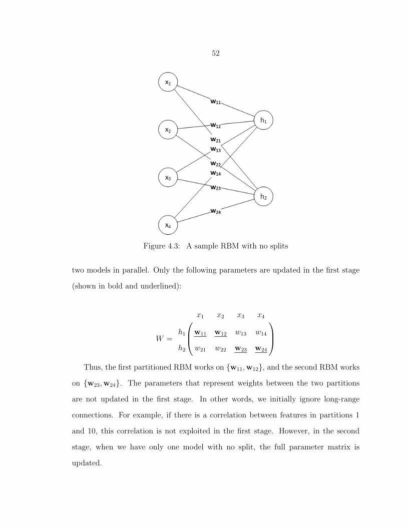
52
Figure 4.3: A sample RBM with no splits
two models in parallel. Only the following parameters are updated in the first stage
(shown in bold and underlined):
W =
x1 x2 x3 x4
h1 w11 w12 w13 w14
h2 w21 w22 w23 w24
Thus, the first partitioned RBM works on w11,w12, and the second RBM works
on w23,w24. The parameters that represent weights between the two partitions
are not updated in the first stage. In other words, we initially ignore long-range
connections. For example, if there is a correlation between features in partitions 1
and 10, this correlation is not exploited in the first stage. However, in the second
stage, when we have only one model with no split, the full parameter matrix is
updated.
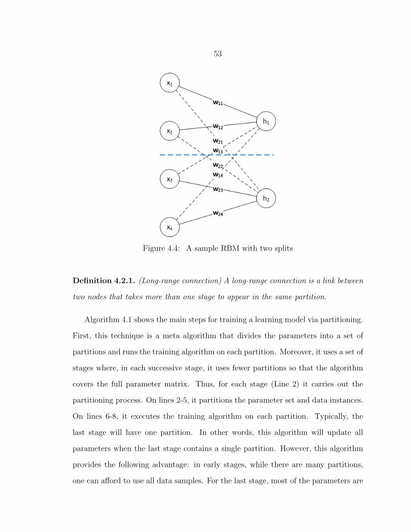
53
Figure 4.4: A sample RBM with two splits
Definition 4.2.1. (Long-range connection) A long-range connection is a link between
two nodes that takes more than one stage to appear in the same partition.
Algorithm 4.1 shows the main steps for training a learning model via partitioning.
First, this technique is a meta algorithm that divides the parameters into a set of
partitions and runs the training algorithm on each partition. Moreover, it uses a set of
stages where, in each successive stage, it uses fewer partitions so that the algorithm
covers the full parameter matrix. Thus, for each stage (Line 2) it carries out the
partitioning process. On lines 2-5, it partitions the parameter set and data instances.
On lines 6-8, it executes the training algorithm on each partition. Typically, the
last stage will have one partition. In other words, this algorithm will update all
parameters when the last stage contains a single partition. However, this algorithm
provides the following advantage: in early stages, while there are many partitions,
one can afford to use all data samples. For the last stage, most of the parameters are
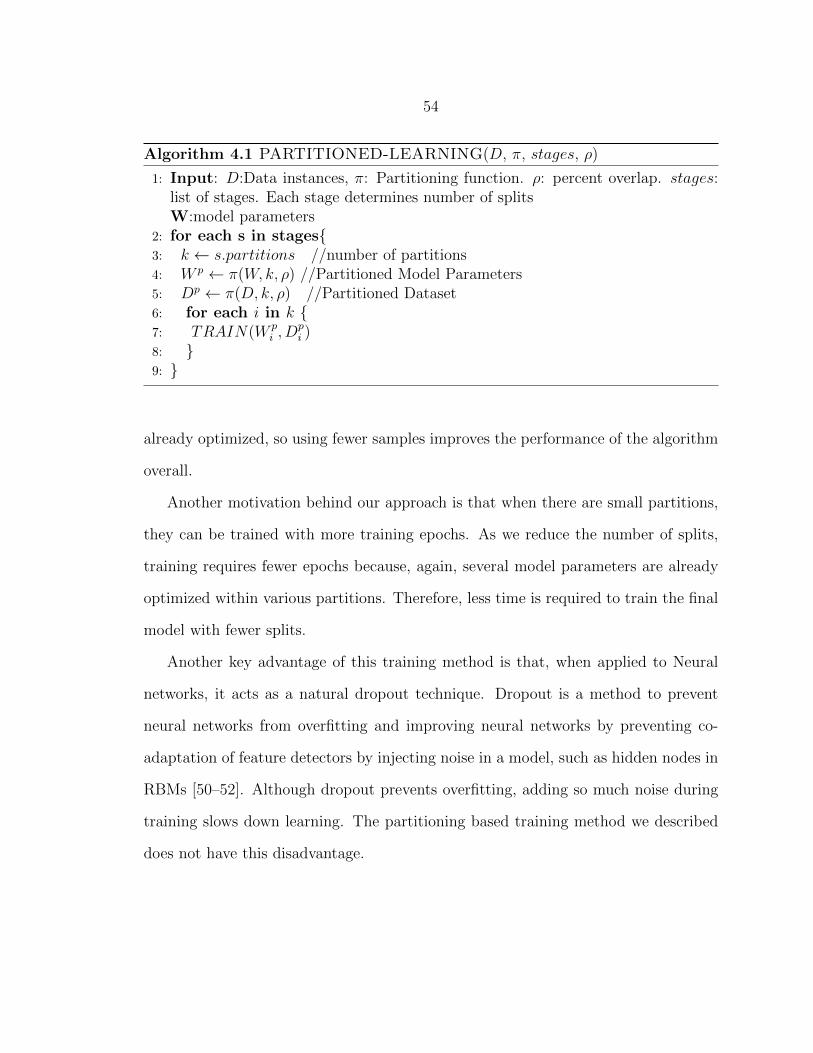
54
Algorithm 4.1 PARTITIONED-LEARNING(D, π, stages, ρ)
1: Input: D:Data instances, π: Partitioning function. ρ: percent overlap. stages:list of stages. Each stage determines number of splitsW:model parameters
2: for each s in stages3: k ← s.partitions //number of partitions4: W p ← π(W,k, ρ) //Partitioned Model Parameters5: Dp ← π(D, k, ρ) //Partitioned Dataset6: for each i in k 7: TRAIN(W p
i , Dpi )
8: 9:
already optimized, so using fewer samples improves the performance of the algorithm
overall.
Another motivation behind our approach is that when there are small partitions,
they can be trained with more training epochs. As we reduce the number of splits,
training requires fewer epochs because, again, several model parameters are already
optimized within various partitions. Therefore, less time is required to train the final
model with fewer splits.
Another key advantage of this training method is that, when applied to Neural
networks, it acts as a natural dropout technique. Dropout is a method to prevent
neural networks from overfitting and improving neural networks by preventing co-
adaptation of feature detectors by injecting noise in a model, such as hidden nodes in
RBMs [50–52]. Although dropout prevents overfitting, adding so much noise during
training slows down learning. The partitioning based training method we described
does not have this disadvantage.
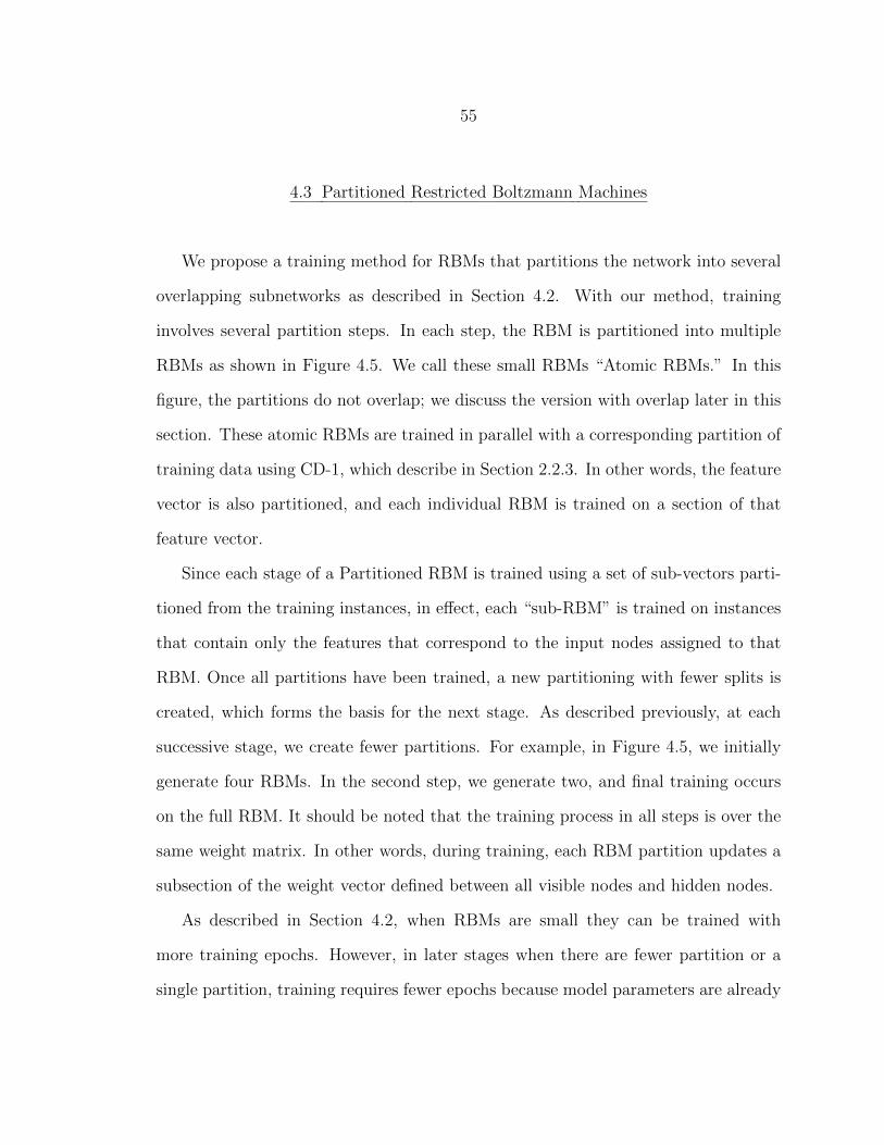
55
4.3 Partitioned Restricted Boltzmann Machines
We propose a training method for RBMs that partitions the network into several
overlapping subnetworks as described in Section 4.2. With our method, training
involves several partition steps. In each step, the RBM is partitioned into multiple
RBMs as shown in Figure 4.5. We call these small RBMs “Atomic RBMs.” In this
figure, the partitions do not overlap; we discuss the version with overlap later in this
section. These atomic RBMs are trained in parallel with a corresponding partition of
training data using CD-1, which describe in Section 2.2.3. In other words, the feature
vector is also partitioned, and each individual RBM is trained on a section of that
feature vector.
Since each stage of a Partitioned RBM is trained using a set of sub-vectors parti-
tioned from the training instances, in effect, each “sub-RBM” is trained on instances
that contain only the features that correspond to the input nodes assigned to that
RBM. Once all partitions have been trained, a new partitioning with fewer splits is
created, which forms the basis for the next stage. As described previously, at each
successive stage, we create fewer partitions. For example, in Figure 4.5, we initially
generate four RBMs. In the second step, we generate two, and final training occurs
on the full RBM. It should be noted that the training process in all steps is over the
same weight matrix. In other words, during training, each RBM partition updates a
subsection of the weight vector defined between all visible nodes and hidden nodes.
As described in Section 4.2, when RBMs are small they can be trained with
more training epochs. However, in later stages when there are fewer partition or a
single partition, training requires fewer epochs because model parameters are already
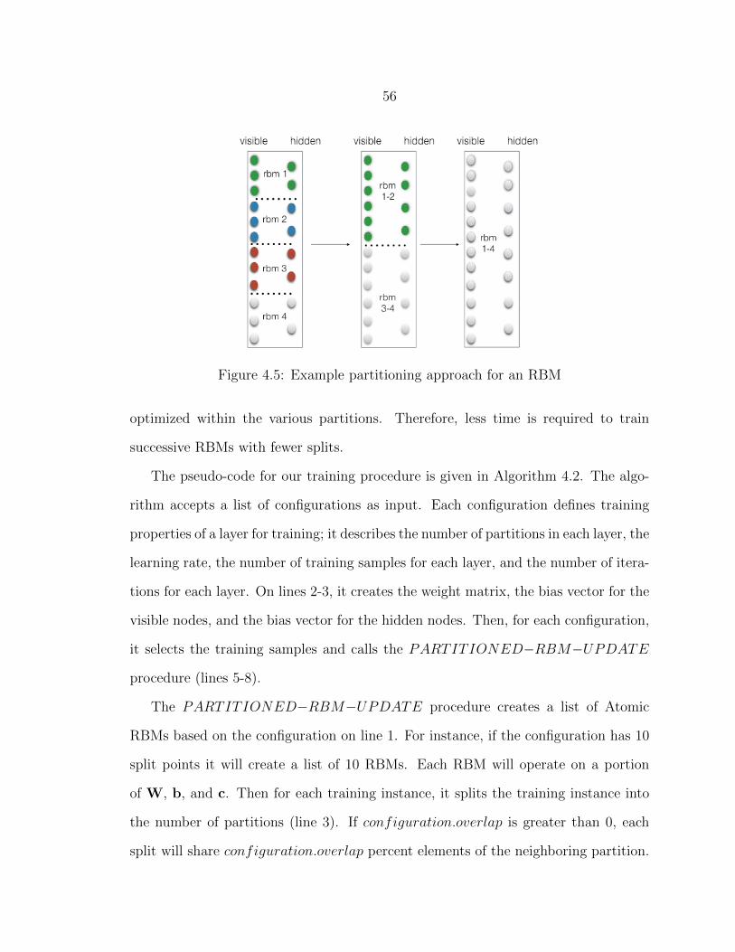
56
Figure 4.5: Example partitioning approach for an RBM
optimized within the various partitions. Therefore, less time is required to train
successive RBMs with fewer splits.
The pseudo-code for our training procedure is given in Algorithm 4.2. The algo-
rithm accepts a list of configurations as input. Each configuration defines training
properties of a layer for training; it describes the number of partitions in each layer, the
learning rate, the number of training samples for each layer, and the number of itera-
tions for each layer. On lines 2-3, it creates the weight matrix, the bias vector for the
visible nodes, and the bias vector for the hidden nodes. Then, for each configuration,
it selects the training samples and calls the PARTITIONED−RBM−UPDATE
procedure (lines 5-8).
The PARTITIONED−RBM−UPDATE procedure creates a list of Atomic
RBMs based on the configuration on line 1. For instance, if the configuration has 10
split points it will create a list of 10 RBMs. Each RBM will operate on a portion
of W, b, and c. Then for each training instance, it splits the training instance into
the number of partitions (line 3). If configuration.overlap is greater than 0, each
split will share configuration.overlap percent elements of the neighboring partition.
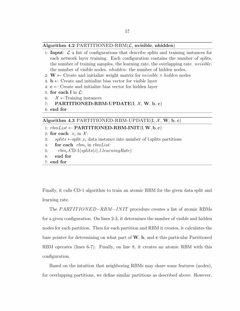
57
Algorithm 4.2 PARTITIONED-RBM(L, nvisible, nhidden)
1: Input: L a list of configurations that describe splits and training instances foreach network layer training. Each configuration contains the number of splits,the number of training samples, the learning rate, the overlapping rate. nvisible:the number of visible nodes. nhidden: the number of hidden nodes.
2: W← Create and initialize weight matrix for nvisible× hidden nodes3: b← Create and initialize bias vector for visible layer4: c← Create and initialize bias vector for hidden layer5: for each l in L:6: X ←Training instances7: PARTITIONED-RBM-UPDATE(l, X , W, b, c)8: end for
Algorithm 4.3 PARTITIONED-RBM-UPDATE(l, X , W, b, c)
1: rbmList← PARTITIONED-RBM-INIT(l,W,b, c)2: for each xi in X :3: splits←split xi data instance into number of l.splits partitions4: for each rbmi in rbmList:5: rbmi.CD-1(splits(i), l.learningRate)6: end for7: end for
Finally, it calls CD-1 algorithm to train an atomic RBM for the given data split and
learning rate.
The PARTITIONED−RBM−INIT procedure creates a list of atomic RBMs
for a given configuration. On lines 2-3, it determines the number of visible and hidden
nodes for each partition. Then for each partition and RBM it creates, it calculates the
base pointer for determining on what part of W, b, and c this particular Partitioned
RBM operates (lines 6-7). Finally, on line 8, it creates an atomic RBM with this
configuration.
Based on the intuition that neighboring RBMs may share some features (nodes),
for overlapping partitions, we define similar partitions as described above. However,
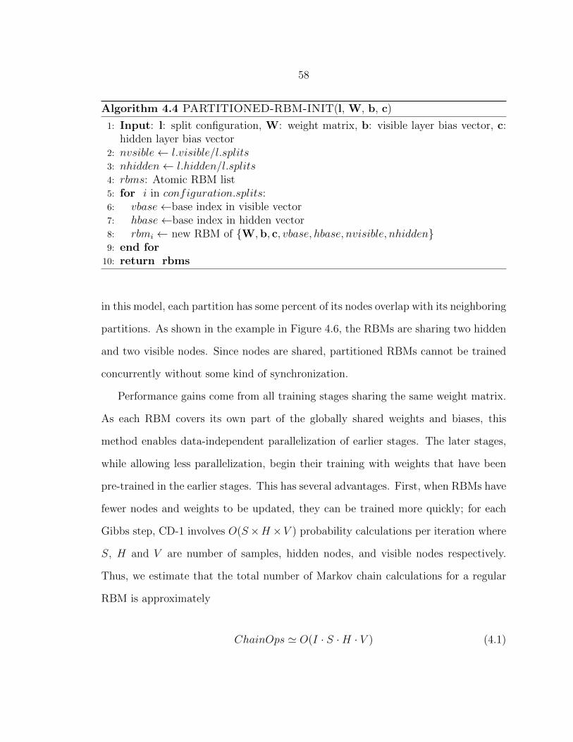
58
Algorithm 4.4 PARTITIONED-RBM-INIT(l, W, b, c)
1: Input: l: split configuration, W: weight matrix, b: visible layer bias vector, c:hidden layer bias vector
2: nvsible← l.visible/l.splits3: nhidden← l.hidden/l.splits4: rbms: Atomic RBM list5: for i in configuration.splits:6: vbase←base index in visible vector7: hbase←base index in hidden vector8: rbmi ← new RBM of W,b, c, vbase, hbase, nvisible, nhidden9: end for10: return rbms
in this model, each partition has some percent of its nodes overlap with its neighboring
partitions. As shown in the example in Figure 4.6, the RBMs are sharing two hidden
and two visible nodes. Since nodes are shared, partitioned RBMs cannot be trained
concurrently without some kind of synchronization.
Performance gains come from all training stages sharing the same weight matrix.
As each RBM covers its own part of the globally shared weights and biases, this
method enables data-independent parallelization of earlier stages. The later stages,
while allowing less parallelization, begin their training with weights that have been
pre-trained in the earlier stages. This has several advantages. First, when RBMs have
fewer nodes and weights to be updated, they can be trained more quickly; for each
Gibbs step, CD-1 involves O(S×H ×V ) probability calculations per iteration where
S, H and V are number of samples, hidden nodes, and visible nodes respectively.
Thus, we estimate that the total number of Markov chain calculations for a regular
RBM is approximately
ChainOps ' O(I · S ·H · V ) (4.1)
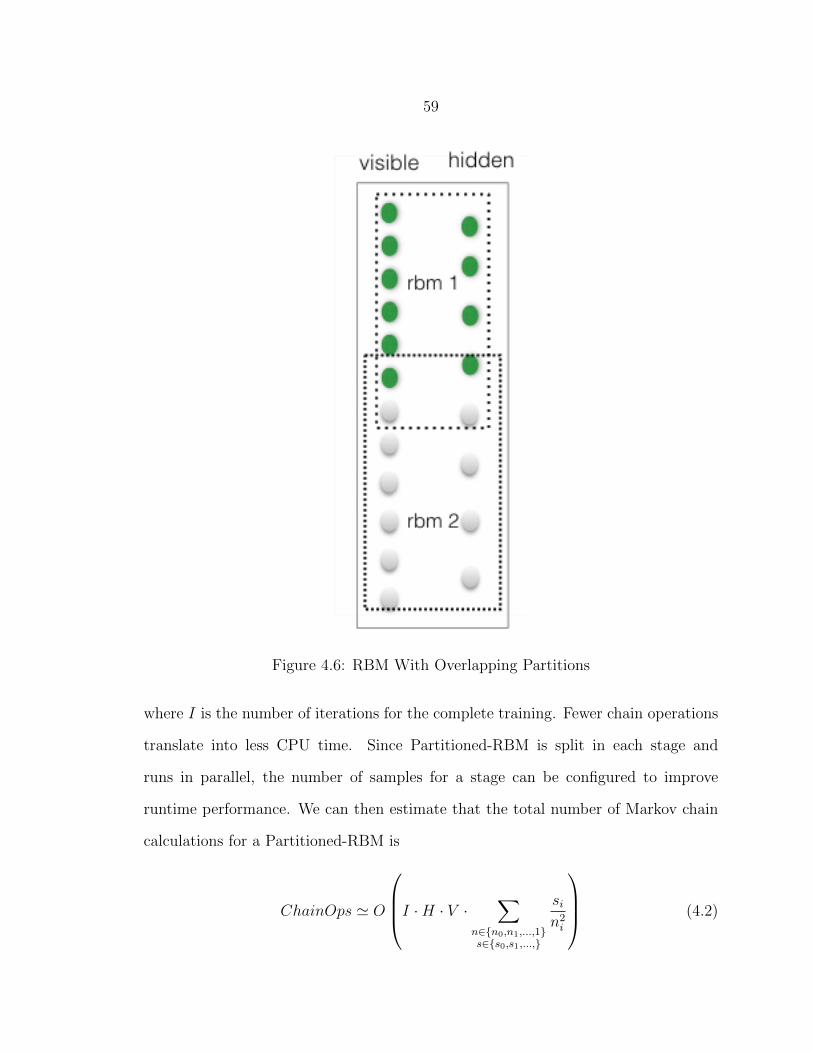
59
Figure 4.6: RBM With Overlapping Partitions
where I is the number of iterations for the complete training. Fewer chain operations
translate into less CPU time. Since Partitioned-RBM is split in each stage and
runs in parallel, the number of samples for a stage can be configured to improve
runtime performance. We can then estimate that the total number of Markov chain
calculations for a Partitioned-RBM is
ChainOps ' O
I ·H · V · ∑n∈n0,n1,...,1s∈s0,s1,...,
sin2i
(4.2)
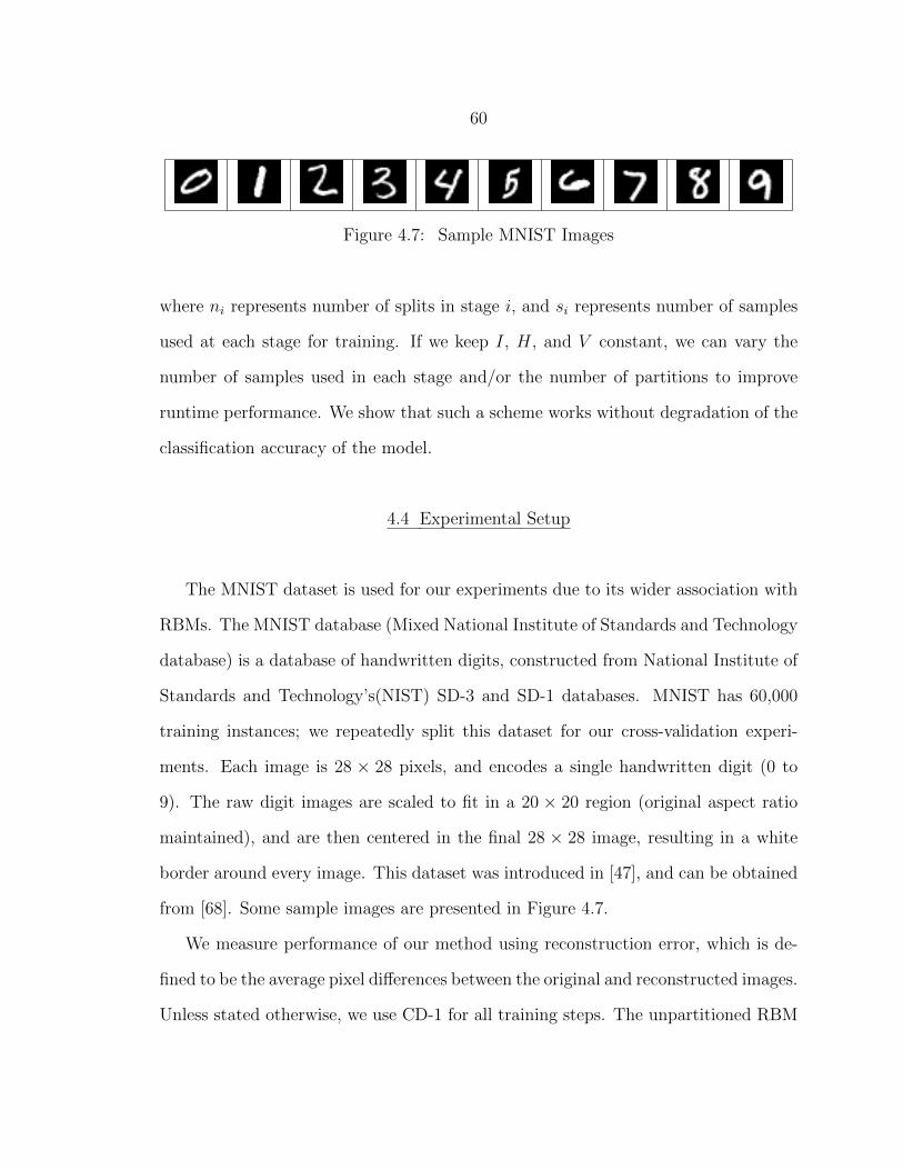
60
Figure 4.7: Sample MNIST Images
where ni represents number of splits in stage i, and si represents number of samples
used at each stage for training. If we keep I, H, and V constant, we can vary the
number of samples used in each stage and/or the number of partitions to improve
runtime performance. We show that such a scheme works without degradation of the
classification accuracy of the model.
4.4 Experimental Setup
The MNIST dataset is used for our experiments due to its wider association with
RBMs. The MNIST database (Mixed National Institute of Standards and Technology
database) is a database of handwritten digits, constructed from National Institute of
Standards and Technology’s(NIST) SD-3 and SD-1 databases. MNIST has 60,000
training instances; we repeatedly split this dataset for our cross-validation experi-
ments. Each image is 28 × 28 pixels, and encodes a single handwritten digit (0 to
9). The raw digit images are scaled to fit in a 20 × 20 region (original aspect ratio
maintained), and are then centered in the final 28 × 28 image, resulting in a white
border around every image. This dataset was introduced in [47], and can be obtained
from [68]. Some sample images are presented in Figure 4.7.
We measure performance of our method using reconstruction error, which is de-
fined to be the average pixel differences between the original and reconstructed images.
Unless stated otherwise, we use CD-1 for all training steps. The unpartitioned RBM
61
has 500 hidden nodes and 28× 28 = 784 visible nodes. CD-1 training for one sample
is carried out as follows:
• For all hidden nodes, find the probability of hidden node hi as σ(ci+∑
jWijxj)
and sample hi1 from a binomial distribution given hi.
• For all visible nodes, find the probability of visible node xj as σ(bj +∑
iWijhi1)
and sample xj1 from a binomial distribution given xj.
• For all hidden nodes, find the probability of hidden node hi2 as σ(ci+∑
jWijxj1).
• Calculate the gradient:
– W = W + ε(hi1xj − h2ixj1) where ε is the learning rate.
– b = b + ε(xj − xj1)
– c = c + ε(hi1 − hi2)
where σ(x) = 11+e−x . Since operations at each step of CD involves visible nodes ×
hidden nodes updates, we estimate that the total number of Markov chain calcula-
tions using Equation 4.1. Fewer chain operations translate into less CPU time.
To get the reconstructed image from the DBN, we propagate the image to the
hidden layer (in case of DBN, all the way to the last hidden layer of Deep Belief
Network), then reconstruct it by reverse propagation to the visible layer. The resulting
vector is binarized and compared with the original vector to calculate a reconstruction
error, E. If x is the original vector, x′ is the reconstruction, and both are of length
n, then E is defined as:
E(x,x′) =1
n
n∑i=1
I(xi 6= x′i) (4.3)
62
For reconstruction error, we first obtain the binary representation of the original
image and the reconstructed image. Thirty is chosen as the threshold for converting
pixel values [0-255] to binary 0 or 1. Thus, pixel values greater than or equal to 30
are set to 1 while values less than 30 are set to 0. Then, the reconstruction error is
calculated as in Equation 4.3.
4.5 Results
Table 4.1 shows the results of our first experiment. Single RBM represents a fully
connected RBM that is used as a baseline for comparison. The learning rate is set
to 0.01 for all RBMs (Single RBM performed best with the learning rate 0.01). The
size of training sample for each RBM is shown in samples column. Unless stated
otherwise, for the following experiments, we ran the training algorithm on samples
for one iteration only—at most, each sample is used only once. Each RBM-X rep-
resents a step with X partitions. Samples chosen for RBM-X are always from the
first N samples of the total images. RBM-1 represents the final model. For these
experiments, partitions are trained sequentially. Thus, if we train them concurrently,
the total ChainOperations will be lower. As compared to Single RBM, RBM-1 has
significantly lower reconstruction error. The total ChainOperations for partitioned
RBMs is also less than Single RBM. In the table, using a t-test, significant results with
99% confidence are shown in bold. Partitioned-RBM after training on 20 partitions,
significantly outperformed the Single RBM. Furthermore, the total number of chain
operations for Partitioned-RBM is substantially less than for Single RBM.
Since we want fast convergence for the first step, in the following experiment
we varied the learning rate to enable this. Results are shown in Table 4.2. The
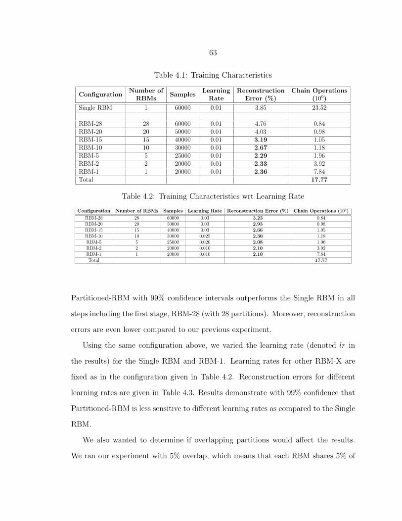
63
Table 4.1: Training Characteristics
ConfigurationNumber of
RBMsSamples
LearningRate
ReconstructionError (%)
Chain Operations(109)
Single RBM 1 60000 0.01 3.85 23.52
RBM-28 28 60000 0.01 4.76 0.84RBM-20 20 50000 0.01 4.03 0.98RBM-15 15 40000 0.01 3.19 1.05RBM-10 10 30000 0.01 2.67 1.18RBM-5 5 25000 0.01 2.29 1.96RBM-2 2 20000 0.01 2.33 3.92RBM-1 1 20000 0.01 2.36 7.84Total 17.77
Table 4.2: Training Characteristics wrt Learning Rate
Configuration Number of RBMs Samples Learning Rate Reconstruction Error (%) Chain Operations (109)
RBM-28 28 60000 0.03 3.23 0.84RBM-20 20 50000 0.03 2.93 0.98RBM-15 15 40000 0.03 2.66 1.05RBM-10 10 30000 0.025 2.30 1.18RBM-5 5 25000 0.020 2.08 1.96RBM-2 2 20000 0.010 2.10 3.92RBM-1 1 20000 0.010 2.10 7.84Total 17.77
Partitioned-RBM with 99% confidence intervals outperforms the Single RBM in all
steps including the first stage, RBM-28 (with 28 partitions). Moreover, reconstruction
errors are even lower compared to our previous experiment.
Using the same configuration above, we varied the learning rate (denoted lr in
the results) for the Single RBM and RBM-1. Learning rates for other RBM-X are
fixed as in the configuration given in Table 4.2. Reconstruction errors for different
learning rates are given in Table 4.3. Results demonstrate with 99% confidence that
Partitioned-RBM is less sensitive to different learning rates as compared to the Single
RBM.
We also wanted to determine if overlapping partitions would affect the results.
We ran our experiment with 5% overlap, which means that each RBM shares 5% of
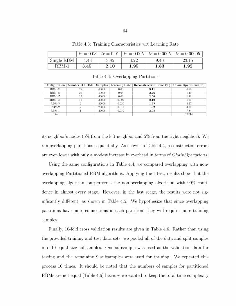
64
Table 4.3: Training Characteristics wrt Learning Rate
lr = 0.03 lr = 0.01 lr = 0.005 lr = 0.0005 lr = 0.00005
Single RBM 4.43 3.85 4.22 9.40 23.15RBM-1 3.45 2.10 1.95 1.83 1.92
Table 4.4: Overlapping Partitions
Configuration Number of RBMs Samples Learning Rate Reconstruction Error (%) Chain Operations(109)
RBM-28 28 60000 0.03 3.11 0.90RBM-20 20 50000 0.03 2.76 1.10RBM-15 15 40000 0.03 2.50 1.18RBM-10 10 30000 0.025 2.19 1.35RBM-5 5 25000 0.020 1.95 2.27RBM-2 2 20000 0.010 1.92 4.30RBM-1 1 20000 0.010 2.08 7.84Total 18.94
its neighbor’s nodes (5% from the left neighbor and 5% from the right neighbor). We
ran overlapping partitions sequentially. As shown in Table 4.4, reconstruction errors
are even lower with only a modest increase in overhead in terms of ChainOperations.
Using the same configurations in Table 4.4, we compared overlapping with non-
overlapping Partitioned-RBM algorithms. Applying the t-test, results show that the
overlapping algorithm outperforms the non-overlapping algorithm with 99% confi-
dence in almost every stage. However, in the last stage, the results were not sig-
nificantly different, as shown in Table 4.5. We hypothesize that since overlapping
partitions have more connections in each partition, they will require more training
samples.
Finally, 10-fold cross validation results are given in Table 4.6. Rather than using
the provided training and test data sets. we pooled all of the data and split samples
into 10 equal size subsamples. One subsample was used as the validation data for
testing and the remaining 9 subsamples were used for training. We repeated this
process 10 times. It should be noted that the numbers of samples for partitioned
RBMs are not equal (Table 4.6) because we wanted to keep the total time complexity
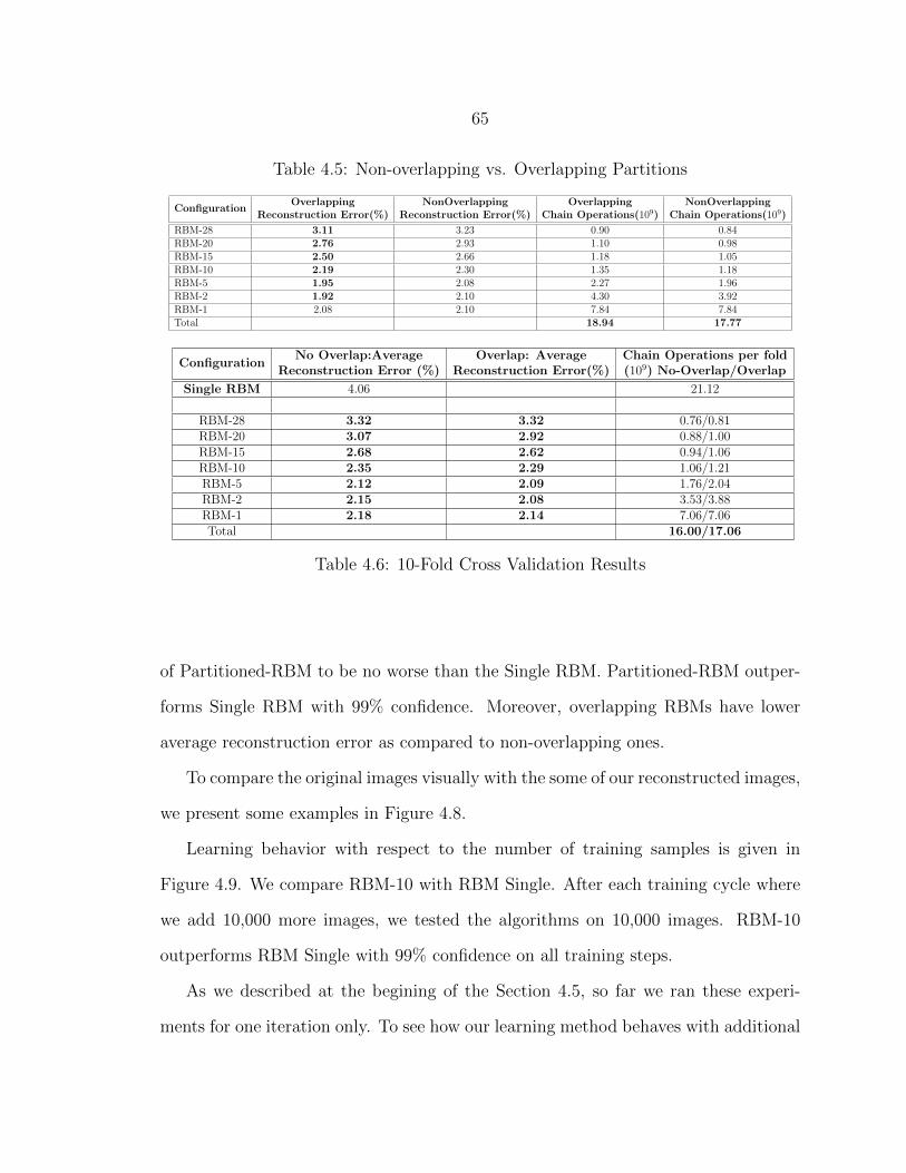
65
Table 4.5: Non-overlapping vs. Overlapping Partitions
ConfigurationOverlapping
Reconstruction Error(%)NonOverlapping
Reconstruction Error(%)Overlapping
Chain Operations(109)NonOverlapping
Chain Operations(109)
RBM-28 3.11 3.23 0.90 0.84RBM-20 2.76 2.93 1.10 0.98RBM-15 2.50 2.66 1.18 1.05RBM-10 2.19 2.30 1.35 1.18RBM-5 1.95 2.08 2.27 1.96RBM-2 1.92 2.10 4.30 3.92RBM-1 2.08 2.10 7.84 7.84Total 18.94 17.77
ConfigurationNo Overlap:Average
Reconstruction Error (%)Overlap: Average
Reconstruction Error(%)Chain Operations per fold(109) No-Overlap/Overlap
Single RBM 4.06 21.12
RBM-28 3.32 3.32 0.76/0.81RBM-20 3.07 2.92 0.88/1.00RBM-15 2.68 2.62 0.94/1.06RBM-10 2.35 2.29 1.06/1.21RBM-5 2.12 2.09 1.76/2.04RBM-2 2.15 2.08 3.53/3.88RBM-1 2.18 2.14 7.06/7.06Total 16.00/17.06
Table 4.6: 10-Fold Cross Validation Results
of Partitioned-RBM to be no worse than the Single RBM. Partitioned-RBM outper-
forms Single RBM with 99% confidence. Moreover, overlapping RBMs have lower
average reconstruction error as compared to non-overlapping ones.
To compare the original images visually with the some of our reconstructed images,
we present some examples in Figure 4.8.
Learning behavior with respect to the number of training samples is given in
Figure 4.9. We compare RBM-10 with RBM Single. After each training cycle where
we add 10,000 more images, we tested the algorithms on 10,000 images. RBM-10
outperforms RBM Single with 99% confidence on all training steps.
As we described at the begining of the Section 4.5, so far we ran these experi-
ments for one iteration only. To see how our learning method behaves with additional
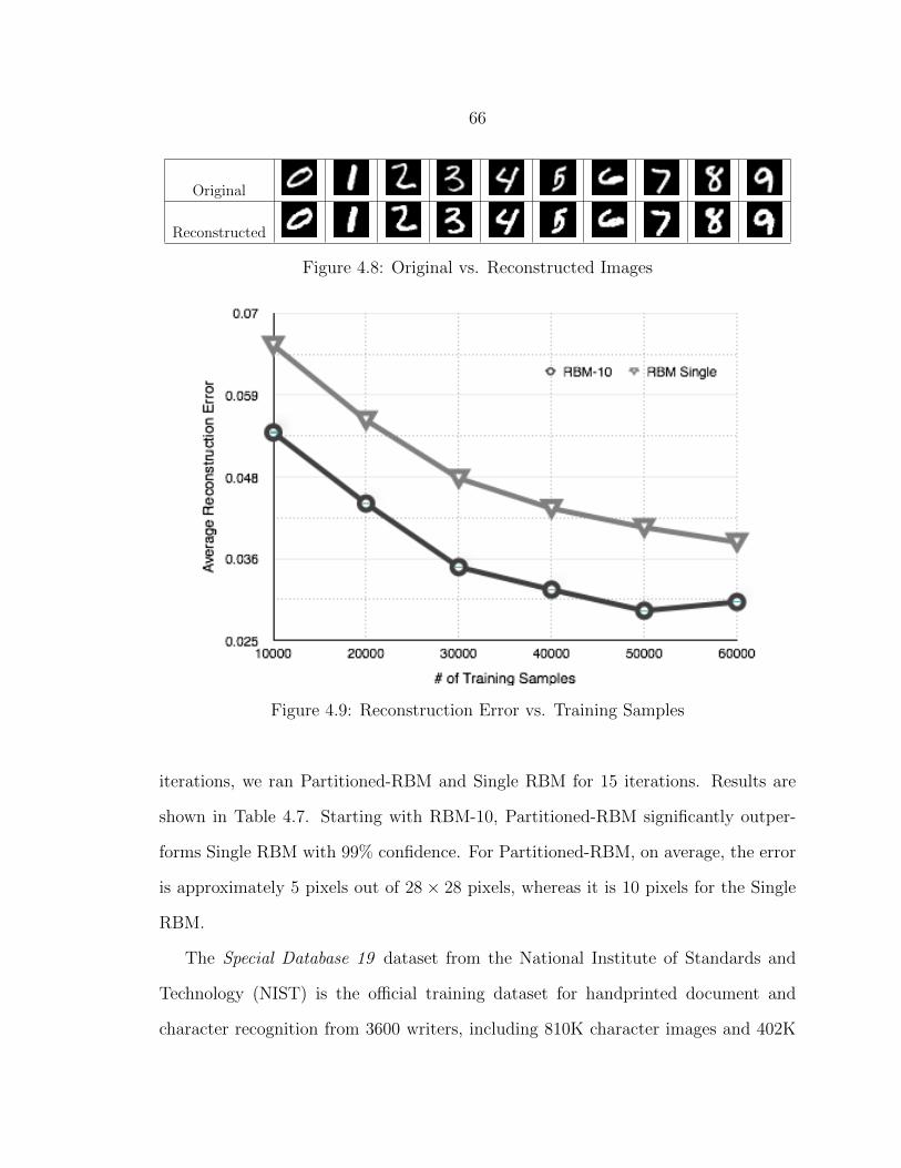
66
Original
Reconstructed
Figure 4.8: Original vs. Reconstructed Images
Figure 4.9: Reconstruction Error vs. Training Samples
iterations, we ran Partitioned-RBM and Single RBM for 15 iterations. Results are
shown in Table 4.7. Starting with RBM-10, Partitioned-RBM significantly outper-
forms Single RBM with 99% confidence. For Partitioned-RBM, on average, the error
is approximately 5 pixels out of 28 × 28 pixels, whereas it is 10 pixels for the Single
RBM.
The Special Database 19 dataset from the National Institute of Standards and
Technology (NIST) is the official training dataset for handprinted document and
character recognition from 3600 writers, including 810K character images and 402K
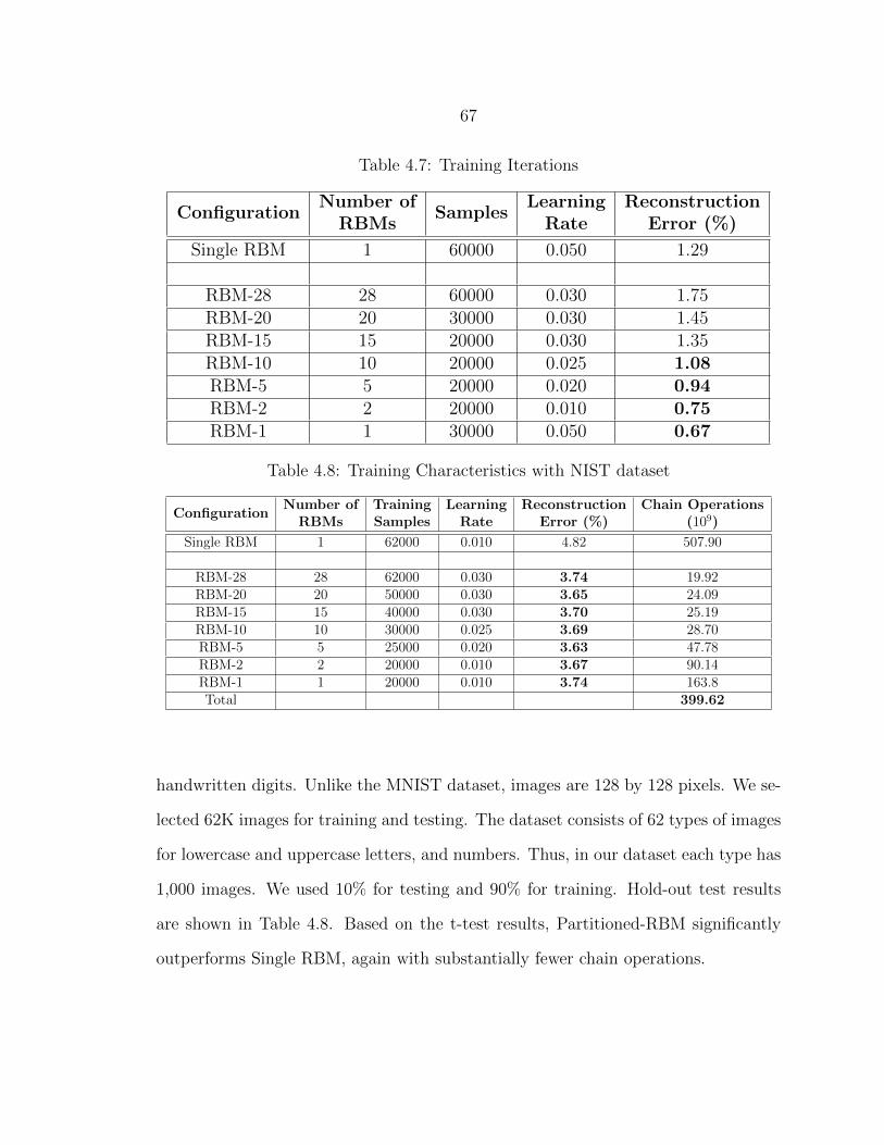
67
Table 4.7: Training Iterations
ConfigurationNumber of
RBMsSamples
LearningRate
ReconstructionError (%)
Single RBM 1 60000 0.050 1.29
RBM-28 28 60000 0.030 1.75RBM-20 20 30000 0.030 1.45RBM-15 15 20000 0.030 1.35RBM-10 10 20000 0.025 1.08RBM-5 5 20000 0.020 0.94RBM-2 2 20000 0.010 0.75RBM-1 1 30000 0.050 0.67
Table 4.8: Training Characteristics with NIST dataset
ConfigurationNumber of
RBMsTrainingSamples
LearningRate
ReconstructionError (%)
Chain Operations(109)
Single RBM 1 62000 0.010 4.82 507.90
RBM-28 28 62000 0.030 3.74 19.92RBM-20 20 50000 0.030 3.65 24.09RBM-15 15 40000 0.030 3.70 25.19RBM-10 10 30000 0.025 3.69 28.70RBM-5 5 25000 0.020 3.63 47.78RBM-2 2 20000 0.010 3.67 90.14RBM-1 1 20000 0.010 3.74 163.8Total 399.62
handwritten digits. Unlike the MNIST dataset, images are 128 by 128 pixels. We se-
lected 62K images for training and testing. The dataset consists of 62 types of images
for lowercase and uppercase letters, and numbers. Thus, in our dataset each type has
1,000 images. We used 10% for testing and 90% for training. Hold-out test results
are shown in Table 4.8. Based on the t-test results, Partitioned-RBM significantly
outperforms Single RBM, again with substantially fewer chain operations.
68
Finally, Partitioned-RBMed reconstruction error for each character is given in
Table 4.9. The average reconstruction error is lowest for I, i, and 1 and it is highest
for W,Q and B.
4.6 Conclusion
We showed that our Partitioned-RBM training algorithm with small RBM par-
titions outperforms training full RBMs using CD-1. In addition to having superior
results in terms of reconstruction error, Partitioned-RBM is also faster as compared to
the single, full RBM. The reason that Partitioned-RBM is faster is due to having fewer
connections in each training step. However, the reasons for the superior generative
characteristics in terms of reconstruction error is due to the fact that it is not trained
fully in the last stage so that weights or feature detectors become uniform. Thus,
it behaves as a dropout. Moreover, we hypothesize that it can also be explained as,
in each training step, fewer nodes are involved and a small partition RBM settles
in a low energy configuration more rapidly. As we move to other stages with less
partitions, fewer training instances are needed to modify the energy configuration to
obtain lower energy in the full network.
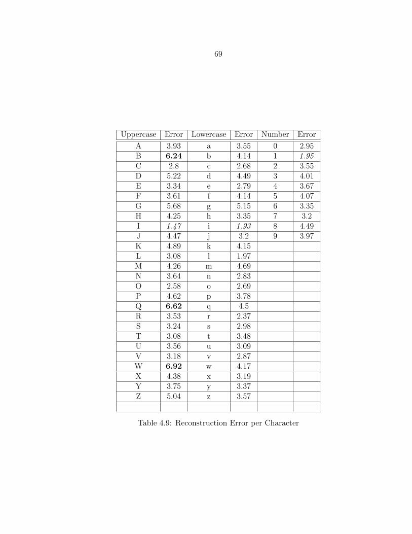
69
Uppercase Error Lowercase Error Number Error
A 3.93 a 3.55 0 2.95B 6.24 b 4.14 1 1.95C 2.8 c 2.68 2 3.55D 5.22 d 4.49 3 4.01E 3.34 e 2.79 4 3.67F 3.61 f 4.14 5 4.07G 5.68 g 5.15 6 3.35H 4.25 h 3.35 7 3.2I 1.47 i 1.93 8 4.49J 4.47 j 3.2 9 3.97K 4.89 k 4.15L 3.08 l 1.97M 4.26 m 4.69N 3.64 n 2.83O 2.58 o 2.69P 4.62 p 3.78Q 6.62 q 4.5R 3.53 r 2.37S 3.24 s 2.98T 3.08 t 3.48U 3.56 u 3.09V 3.18 v 2.87W 6.92 w 4.17X 4.38 x 3.19Y 3.75 y 3.37Z 5.04 z 3.57
Table 4.9: Reconstruction Error per Character
70
CHAPTER 5
PARTITIONED DISCRIMINATIVE NETWORKS
Recently, researchers have shown an increased interest in considering Restricted
Boltzmann Machines (RBMs) as a standalone classifiers; however, many researchers
have only aimed at obtaining higher recall and precision of the learning model. So
far, there has been little discussion about runtime performance. In this chapter,
we introduce a partitioned based RBM for classification tasks. The objective of this
chapter is to evaluate the classification accuracy of Partitioned-RBMs under bounded
resources.
5.1 Discriminative Restricted Boltzmann Machines
Larochelle et al. carried out a comprehensive study of RBMs in classification tasks
and successfully applied RBMs as a standalone learning technique, which they call
classRBM [70]. In addition to a generative training objective function for the CD
algorithm, the authors developed a discriminative training objective function as well.
Furthermore, combining these two objective functions, they created a hybrid objective
function that was then used for the gradient calculations. The authors reported that
the hybrid method produced excellent results; however, we could not replicate their
results because the discriminative training objective function calculations resulted
in an overflow for reasonably large networks. The following objective function is a
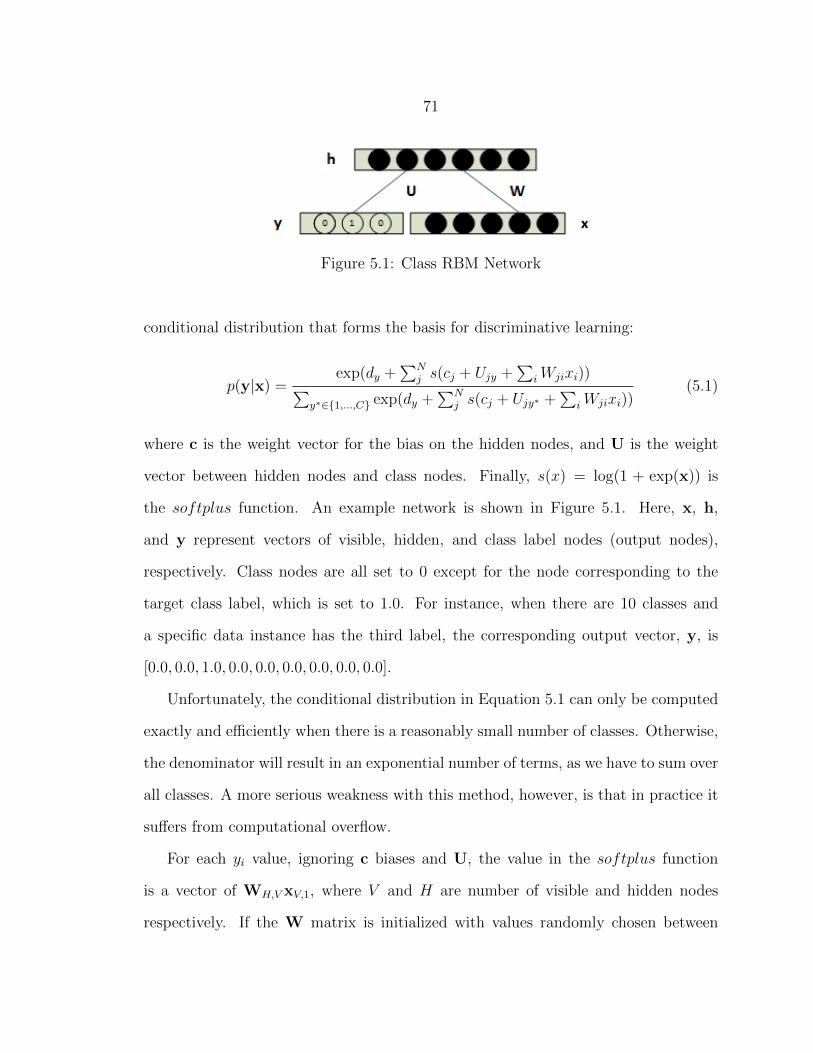
71
Figure 5.1: Class RBM Network
conditional distribution that forms the basis for discriminative learning:
p(y|x) =exp(dy +
∑Nj s(cj + Ujy +
∑iWjixi))∑
y∗∈1,...,C exp(dy +∑N
j s(cj + Ujy∗ +∑
iWjixi))(5.1)
where c is the weight vector for the bias on the hidden nodes, and U is the weight
vector between hidden nodes and class nodes. Finally, s(x) = log(1 + exp(x)) is
the softplus function. An example network is shown in Figure 5.1. Here, x, h,
and y represent vectors of visible, hidden, and class label nodes (output nodes),
respectively. Class nodes are all set to 0 except for the node corresponding to the
target class label, which is set to 1.0. For instance, when there are 10 classes and
a specific data instance has the third label, the corresponding output vector, y, is
[0.0, 0.0, 1.0, 0.0, 0.0, 0.0, 0.0, 0.0, 0.0].
Unfortunately, the conditional distribution in Equation 5.1 can only be computed
exactly and efficiently when there is a reasonably small number of classes. Otherwise,
the denominator will result in an exponential number of terms, as we have to sum over
all classes. A more serious weakness with this method, however, is that in practice it
suffers from computational overflow.
For each yi value, ignoring c biases and U, the value in the softplus function
is a vector of WH,V xV,1, where V and H are number of visible and hidden nodes
respectively. If the W matrix is initialized with values randomly chosen between
72
−1.0maxV,H and +1.0
maxV,H and for H = 1500 and V = 784, the resulting matrix values
will be distributed uniformly between −0.00067 and 0.00067. Thus, the value for
exp(∗) in softplus function ranges from 0.9993 to 1.0007. The log(1 + ∗) expression
results in values around 0.69. Then, ignoring dy, the∑
(∗) expression has value of
H × 0.69. Finally, it results in exp(H × 0.69). Thus, with H = 1500, we have
exp(1035). For modern CPUs, exp(710.0) results in overflow (infinity). Therefore,
the maximum number of hidden nodes one can use is around 710.0/0.69, that is 1028
nodes.
It should be noted that we ignored many variables in this formula to simplify
the analysis. Thus, even for 1028 nodes, it is not guaranteed that the overflow will
not happen. Overflow can be encountered when one uses fewer than 1000 nodes. In
addition to the overflow, the time complexity of an RBM increases with addition of
the discriminative gradient.
Because we could not use classRBM for some reasonably sized experiments, here
we propose a model where we train partitions as described in Chapter 4 without using
class labels except for the last stage. As shown in Figure 5.2, class nodes are added
to the visible vector of the final stage with one node per class. Thus, we train the
final stage in a supervised fashion.
5.2 Discriminative Partitioned Restricted Boltzmann Machines
For discriminative RBMs, we propose the Partitioned Restricted Boltzmann Ma-
chine (PRBM) model where we train partitions as described in Chapter 4 without
using class labels except for the last layer. As shown in Figure 5.2, class nodes are
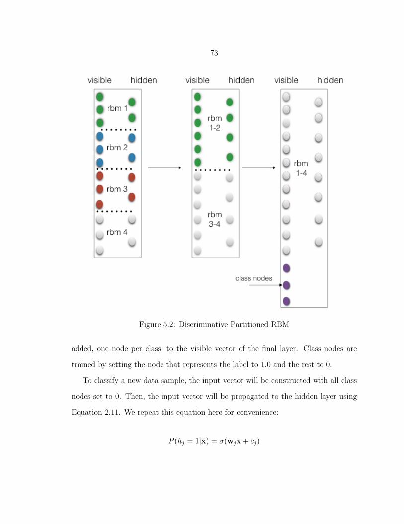
73
Figure 5.2: Discriminative Partitioned RBM
added, one node per class, to the visible vector of the final layer. Class nodes are
trained by setting the node that represents the label to 1.0 and the rest to 0.
To classify a new data sample, the input vector will be constructed with all class
nodes set to 0. Then, the input vector will be propagated to the hidden layer using
Equation 2.11. We repeat this equation here for convenience:
P (hj = 1|x) = σ(wjx + cj)
74
A new visible vector will be sampled from the model based on the activation of hidden
nodes. Since the visible vector contains class nodes as well, the class nodes’ values
will be used to predict the class label. The class node with the highest activation
value will determine the class label.
Because PRBM is partitioned into smaller RBMs, all available data can be used for
training, and individual RBMs can be trained in parallel. Moreover, as the number
of dimensions increases, the number of partitions can be increased to reduce run-
time computational resource requirements significantly. All other recently developed
methods using RBMs for classification suffer from some serious disadvantage under
bounded computational resources; one is forced either to use a subsample of the
whole data, run fewer iterations (early stop criterion), or both. Our Partitioned-
RBM method provides an innovative scheme to overcome these shortcomings.
As proposed in Chapter 4, the training process for Partitioned-RBM splits a single
RBM into multiple partitions. Each partition is then trained on a subsection of
the data instances. In our experiments, we demonstrated that this training process
improves the performance in terms of both generative power and speed. Moreover,
we will show in Chapter 6, applying spatial statistical analysis tools, we found that
traditional RBMs do not preserve spatially local structure whereas Partitioned-RBMs
are preserve and make use of local structure [69].
We believe that far too little attention has been paid to runtime performance
and far too much attention has been paid to obtaining higher classification accuracy
rates. To the best of our knowledge, using RBMs with bounded computational re-
sources, namely CPU time, has not been considered previously. Hence, the goal of
this chapter is to find out if there exists a method for improving the runtime per-
formance of RBMs without significantly degrading classification accuracy. When we
developed the Partitioned-RBM to obtain better reconstruction accuracy, we noticed
75
that runtime performance is also superior to regular RBMs [5]. Thus, our previous re-
sults suggest that Partitioned-RBMs can perform significantly better under bounded
computational resources.
Another key aspect of our Partitioned-RBM is that the training process introduces
an intrinsic sparsity by design. At each training stage, only the weights inside individ-
ual partitions are optimized; the weights connecting the visible layer of one partition
to the hidden layer of another partition are untouched. Thus, the Partitioned-RBM
weights are inherently sparse. This is important because Larochelle et al. showed
that a sparse version of the hybrid RBM significantly outperforms all other tech-
niques in terms of classification error rates; the results were even better than Deep
Belief Network results reported in the literature [25]. Larochelle et al. introduced
sparsity by subtracting a small constant δ value, a hyper-parameter, from biases after
each parameter update. In our case, the training of smaller partitions and gradually
piecing them together accomplishes a similar result.
Algorithm 5.1 is a slightly modified version of the CD-1 training technique for
classification tasks. On line 2-6, we calculate hidden node activations. When the
training is done for the classification (when there are class nodes), we add the con-
tribution of the class input nodes by multiplying with the U matrix. In other words,
the squashing function that calculates hidden node activations, in addition to Wx,
has the Uy component. On line 7, new values for h are sampled from the hidden
activations. Using sampled h values, the new values for x and y are calculated on
lines 8-11. Using new predicted values of x and y, new hidden activation probabil-
ities are obtained on lines 12-16. Depending on whether the network is trained for
classification or not, the contribution of Uy is added to the probability calculations
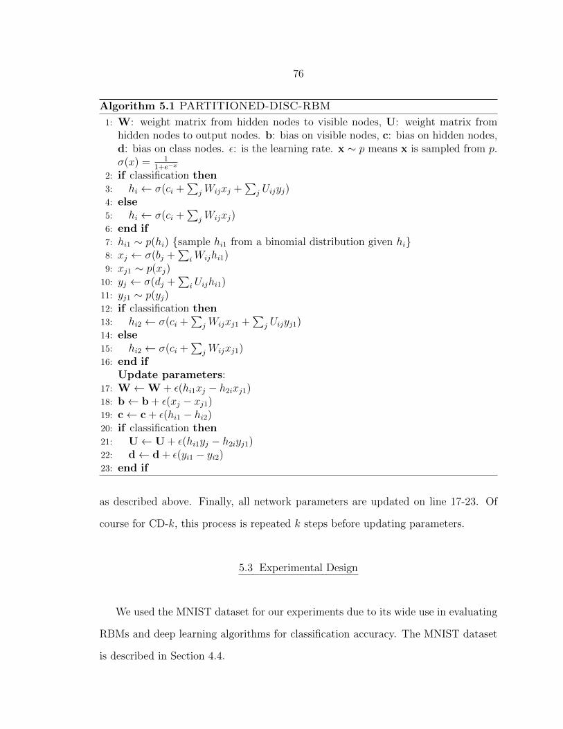
76
Algorithm 5.1 PARTITIONED-DISC-RBM
1: W: weight matrix from hidden nodes to visible nodes, U: weight matrix fromhidden nodes to output nodes. b: bias on visible nodes, c: bias on hidden nodes,d: bias on class nodes. ε: is the learning rate. x ∼ p means x is sampled from p.σ(x) = 1
1+e−x
2: if classification then3: hi ← σ(ci +
∑jWijxj +
∑j Uijyj)
4: else5: hi ← σ(ci +
∑jWijxj)
6: end if7: hi1 ∼ p(hi) sample hi1 from a binomial distribution given hi8: xj ← σ(bj +
∑iWijhi1)
9: xj1 ∼ p(xj)10: yj ← σ(dj +
∑i Uijhi1)
11: yj1 ∼ p(yj)12: if classification then13: hi2 ← σ(ci +
∑jWijxj1 +
∑j Uijyj1)
14: else15: hi2 ← σ(ci +
∑jWijxj1)
16: end ifUpdate parameters:
17: W←W + ε(hi1xj − h2ixj1)18: b← b + ε(xj − xj1)19: c← c + ε(hi1 − hi2)20: if classification then21: U← U + ε(hi1yj − h2iyj1)22: d← d + ε(yi1 − yi2)23: end if
as described above. Finally, all network parameters are updated on line 17-23. Of
course for CD-k, this process is repeated k steps before updating parameters.
5.3 Experimental Design
We used the MNIST dataset for our experiments due to its wide use in evaluating
RBMs and deep learning algorithms for classification accuracy. The MNIST dataset
is described in Section 4.4.
77
Rather than using the pre-defined test set of 10,000 images, we repeatedly split
the training dataset for our cross-validation experiments. Unless stated otherwise,
for all experiments, we trained models for 20 iterations. Moreover, when we compare
methods in terms of the significance of results, we compare them using a paired t-test
with 99% confidence intervals.
5.4 Results
Table 5.1 shows the results of our Partitioned-RBM experiments with 1500 hidden
nodes. In the configuration column, Single RBM represents the traditional RBM and
Partitioned-RBM represents a Partitioned RBM. The number of partitions in each
training stage is defined in parentheses; (16-4-1) indicates that we trained the RBM
first with 16 splits, then 4, and finally trained it as a single partition. Note that
each successive Partitioned-RBM configuration starts with the output of the previous
configuration, as described in Chapter 4. The Samples column gives the number of
training instances, selected at random from the total training set, that were used to
train the given RBM. As the number of partitions decreases, we decrease the training
set size to match the time complexity of the full Partitioned-RBM training process to
that of the Single RBM. Each RBM was run for 20 iterations, and the classification
accuracy rates reported are the mean values from 10-fold cross-validation (not using
MNIST’s predefined split between training and test data). As shown, Partitioned-
RBM significantly outperforms the Single RBM.
By design, the computational complexity of the Partitioned-RBM is significantly
better than that of the Single RBM trained on the entire dataset; it is evident that less
computation would have been necessary for the Partitioned-RBM to yield superior
performance. Based on Equation 4.2 (repeated below for convenience) we could tune
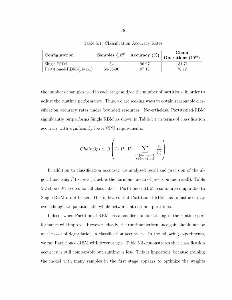
78
Table 5.1: Classification Accuracy Rates
Configuration Samples (103) Accuracy (%)Chain
Operations (1010)
Single RBM 54 96.97 131.71Partitioned-RBM-(16-4-1) 54-50-30 97.18 78.42
the number of samples used in each stage and/or the number of partitions, in order to
adjust the runtime performance. Thus, we are seeking ways to obtain reasonable clas-
sification accuracy rates under bounded resources. Nevertheless, Partitioned-RBM
significantly outperforms Single RBM as shown in Table 5.1 in terms of classification
accuracy with significantly lower CPU requirements.
ChainOps ' O
I ·H · V · ∑n∈n0,n1,...,1s∈s0,s1,...,
sin2i
In addition to classification accuracy, we analyzed recall and precision of the al-
gorithms using F1 scores (which is the harmonic mean of precision and recall). Table
5.2 shows F1 scores for all class labels. Partitioned-RBM results are comparable to
Single RBM if not better. This indicates that Partitioned-RBM has robust accuracy
even though we partition the whole network into atomic partitions.
Indeed, when Partitioned-RBM has a smaller number of stages, the runtime per-
formance will improve. However, ideally, the runtime performance gain should not be
at the cost of degradation in classification accuracies. In the following experiments,
we ran Partitioned-RBM with fewer stages. Table 5.3 demonstrates that classification
accuracy is still comparable but runtime is less. This is important, because training
the model with many samples in the first stage appears to optimize the weights
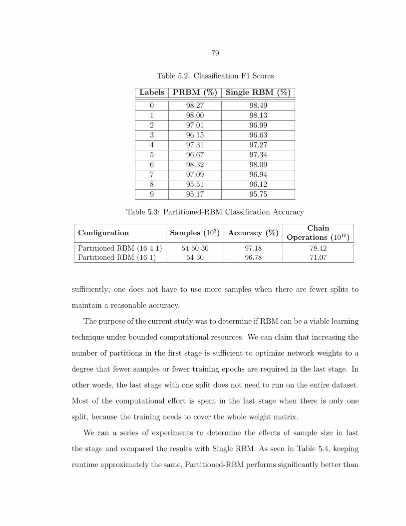
79
Table 5.2: Classification F1 Scores
Labels PRBM (%) Single RBM (%)
0 98.27 98.491 98.00 98.132 97.01 96.993 96.15 96.634 97.31 97.275 96.67 97.346 98.32 98.097 97.09 96.948 95.51 96.129 95.17 95.75
Table 5.3: Partitioned-RBM Classification Accuracy
Configuration Samples (103) Accuracy (%)Chain
Operations (1010)
Partitioned-RBM-(16-4-1) 54-50-30 97.18 78.42Partitioned-RBM-(16-1) 54-30 96.78 71.07
sufficiently; one does not have to use more samples when there are fewer splits to
maintain a reasonable accuracy.
The purpose of the current study was to determine if RBM can be a viable learning
technique under bounded computational resources. We can claim that increasing the
number of partitions in the first stage is sufficient to optimize network weights to a
degree that fewer samples or fewer training epochs are required in the last stage. In
other words, the last stage with one split does not need to run on the entire dataset.
Most of the computational effort is spent in the last stage when there is only one
split, because the training needs to cover the whole weight matrix.
We ran a series of experiments to determine the effects of sample size in last
the stage and compared the results with Single RBM. As seen in Table 5.4, keeping
runtime approximately the same, Partitioned-RBM performs significantly better than
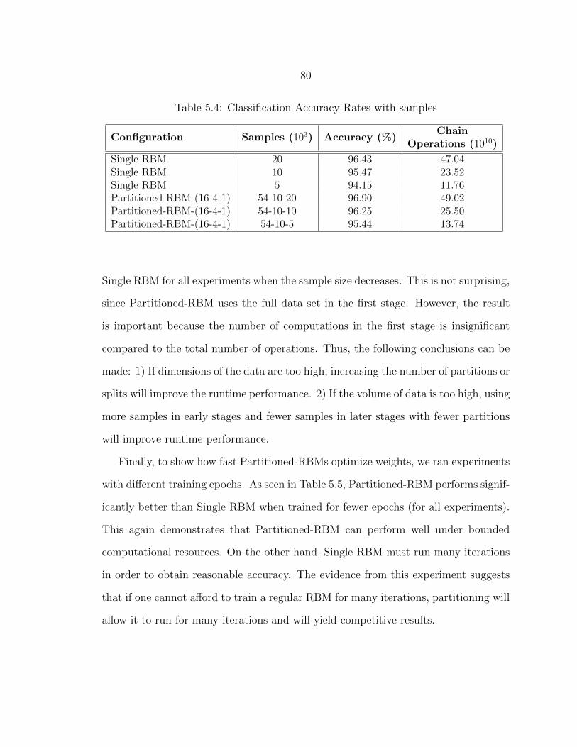
80
Table 5.4: Classification Accuracy Rates with samples
Configuration Samples (103) Accuracy (%)Chain
Operations (1010)
Single RBM 20 96.43 47.04Single RBM 10 95.47 23.52Single RBM 5 94.15 11.76Partitioned-RBM-(16-4-1) 54-10-20 96.90 49.02Partitioned-RBM-(16-4-1) 54-10-10 96.25 25.50Partitioned-RBM-(16-4-1) 54-10-5 95.44 13.74
Single RBM for all experiments when the sample size decreases. This is not surprising,
since Partitioned-RBM uses the full data set in the first stage. However, the result
is important because the number of computations in the first stage is insignificant
compared to the total number of operations. Thus, the following conclusions can be
made: 1) If dimensions of the data are too high, increasing the number of partitions or
splits will improve the runtime performance. 2) If the volume of data is too high, using
more samples in early stages and fewer samples in later stages with fewer partitions
will improve runtime performance.
Finally, to show how fast Partitioned-RBMs optimize weights, we ran experiments
with different training epochs. As seen in Table 5.5, Partitioned-RBM performs signif-
icantly better than Single RBM when trained for fewer epochs (for all experiments).
This again demonstrates that Partitioned-RBM can perform well under bounded
computational resources. On the other hand, Single RBM must run many iterations
in order to obtain reasonable accuracy. The evidence from this experiment suggests
that if one cannot afford to train a regular RBM for many iterations, partitioning will
allow it to run for many iterations and will yield competitive results.
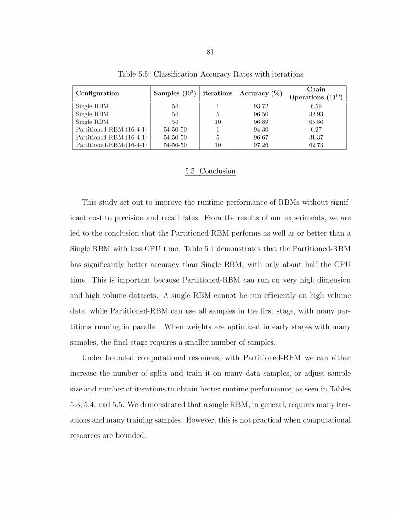
81
Table 5.5: Classification Accuracy Rates with iterations
Configuration Samples (103) iterations Accuracy (%)Chain
Operations (1010)
Single RBM 54 1 93.72 6.59Single RBM 54 5 96.50 32.93Single RBM 54 10 96.89 65.86Partitioned-RBM-(16-4-1) 54-50-50 1 94.30 6.27Partitioned-RBM-(16-4-1) 54-50-50 5 96.67 31.37Partitioned-RBM-(16-4-1) 54-50-50 10 97.26 62.73
5.5 Conclusion
This study set out to improve the runtime performance of RBMs without signif-
icant cost to precision and recall rates. From the results of our experiments, we are
led to the conclusion that the Partitioned-RBM performs as well as or better than a
Single RBM with less CPU time. Table 5.1 demonstrates that the Partitioned-RBM
has significantly better accuracy than Single RBM, with only about half the CPU
time. This is important because Partitioned-RBM can run on very high dimension
and high volume datasets. A single RBM cannot be run efficiently on high volume
data, while Partitioned-RBM can use all samples in the first stage, with many par-
titions running in parallel. When weights are optimized in early stages with many
samples, the final stage requires a smaller number of samples.
Under bounded computational resources, with Partitioned-RBM we can either
increase the number of splits and train it on many data samples, or adjust sample
size and number of iterations to obtain better runtime performance, as seen in Tables
5.3, 5.4, and 5.5. We demonstrated that a single RBM, in general, requires many iter-
ations and many training samples. However, this is not practical when computational
resources are bounded.

82
One might ask why we did not add class nodes in early stages. Our initial results
indicated that such a scheme does not provide any advantage. It appears that when
weights between hidden nodes and class nodes, U, are updated by all partitions, the
weight matrix takes a long time to be optimized; one partition changes the effect of a
previous partition. However, we plan to investigate each partition optimizing its own
U matrix, and, we need to find a better mechanism to combine all U matrices when
we move to the next stage in the training process.
83
CHAPTER 6
PARTITIONED DEEP BELIEF NETWORKS
To show how the performance can be improved while simultaneously decreasing
total training time, a DBN composed of the Restricted Boltzmann Machines (RBMs)
will be explored next. We present this by introducing the vector-partitioning de-
scribed in Chapter 4. We then analyze the input data to see if we can identify the
statistical properties that are being exploited by the Partitioned-RBM to achieve
this performance. Our goal is to investigate the representation bias of the deep,
vector-partitioning approaches in general. Examination of that bias is critical to
understanding and improving our learning algorithms, as Tom Mitchell pointed out
in his seminal paper [71], in which he also noted that a bias necessary for learning.
Moreover, we analyze the role of spatial locality in Deep Belief Networks (DBN) and
show that spatially local information becomes diffused as the network becomes deeper.
We demonstrate that our method is capable of retaining spatially local information
when training DBNs. Specifically, we find that spatially local features are completely
lost in DBNs trained using the “standard” RBM method, but are largely preserved
using our partitioned training method. In addition, reconstruction accuracy of the
model is improved using our Partitioned-RBM training method.
6.1 Deep Belief Networks with Partitioned Restricted Boltzmann Machines
In the past few years, the area of exploration known as Deep Learning has demon-
strated the ability of multilayer networks to achieve good performance on a range
of difficult machine learning problems and has been gaining increasing prominence
84
and attention in the machine learning and neural network communities and rapid
adoption in commercial products. While these techniques have achieved great suc-
cess on a number of difficult classification problems, for example in computer vision,
the role of representation bias has not been thoroughly explored. In other words, we
do not know the underlying reasons why these techniques perform well on particular
problems. A deeper understanding of how and why deep learning algorithms work
will help us to decide which problems they are best applied to, and may also lead to
improvement of existing techniques or extending them to in novel contexts.
We demonstrated in Chapters 4 and 5 that partitioned learning can be applied
effectively to RBMs. Here, we apply that same thought to deep learning. As a first
step to examine the role of representation bias, we use statistical models to examine
how much spatially local structure exists in the MNIST dataset. We then present
experimental results from training RBMs using partitioned data and demonstrate
the advantages they have over non-partitioned RBMs. Through these results, we
show how this performance advantage depends on spatially local structure by demon-
strating the performance impact of randomly permuting the input data to destroy
local structure. Overall, our results support the hypothesis that a representation bias
relying on spatially local statistical information can improve performance if this bias
is a good match for the data. We also suggest statistical tools for determining a priori
whether a dataset has spatially local features that will make it a good match for this
bias.
The question we want to answer is, “Do deep learning algorithms make use of
spatially local structure in their input data to help them achieve good performance?”
There has long been an intuition in the deep learning community that this hypothesis
is likely to hold, based partly on everyday experience, and partly on the structure
85
of the human visual cortex. To our knowledge, however, there has been no previous
attempt to test this hypothesis.
Deep networks have a built-in regularization effect that remains strong even when
working with large amounts of data [34]. This gives them an advantage on data
with noise or complexities resembling noise. In addition, for partitioned deep models
like Convolutional Networks, exploiting spatially local information is important to
performance [35].
Partitioned deep models work by partitioning nodes within layers of a network.
As shown in Figure 4.5, this can be visualized as an RBM in which layers are not fully
connected. Instead, the nodes of each layer are broken into subsets, and each subset
of nodes is fully connected. As an example, in a classic Convolutional Networks, a
data vector represents an input (e.g. an image) and is effectively split into several
small overlapping regions (image patches).
In a typical DBN, a Restricted Boltzman Machine is at each layer and the network
is trained layer-wise by non-linearly transforming the input while minimizing recon-
struction error. Once all layers have been trained, the resultant network can then be
used in different ways, including adding a new output layer and running a standard
gradient descent algorithm to learn a supervised task such as classification. We use the
same architecture and training process; however, instead of using a monolithic RBM,
we use Partitioned-RBMs and carry out the partitioned training process described in
Chapter 4 at each layer of the DBN.
Performance gains come from all training stages sharing the same weight matrix.
As each RBM covers its own part of the globally shared weights and biases, this
method enables data-independent parallelization of earlier stages.1 The later stages,
1If we allow for overlap of partitions, parallelization becomes problematic. However, Fortier etal. suggest an approach that enables parallelization while exploiting overlap [72–74].
86
while allowing less parallelization, begin their training with weights that have been
pre-trained by the earlier stages. This has several advantages. First, when RBMs have
fewer nodes and weights to be updated, they can be trained more quickly. While the
results of the disjoint training will not be perfect because some relationships will be
missing, they can be allowed to run for many epochs and on large dataset. At the
later stages, as the RBMs cover more links, the training requires fewer epochs than
normal to converge because the weights are closer to their optimal values than would
be the case with random initialization. This enables the overall Partitioned-RBM
hierarchy to achieve the same or higher performance in a fixed time period than a
single RBM trained all at once.
This type of partitioning method can have detrimental effects on performance.
After all, any statistical information relating two features that are not contained in
the same partition is completely hidden from the model. In practice, however, for
most real-world problems, we have neither enough samples nor the computational
capacity to generate a fully optimal statistical model of our data. Most of the models
we are interested in yield exponential complexities, so we must rely on approximations
to estimate them. The central issue in neural networks, going back to McCulloch and
Pitts [75], is the intractability of finding the optimal set of connection weights. The
history of the field has largely been a progressive improvement of gradient descent-
based approximation algorithms, which have enabled more complex network architec-
tures to be trained. Simplifying assumptions often allow more tractable approaches
to problem solving, but assumptions made should be consistent with the original
problem.
We suggest that deep learning algorithms, and in particular the ones that partition
data vectors, are taking advantage of spatially local statistical structure for their
performance. This requires not only that such structure exists, but that it be highly
87
relevant to the performance criterion being optimized. If this hypothesis is correct,
it means we may be able to exploit this structure in other contexts as well.
We can now describe the statistical properties of random variables across the
dataset. For individual features, we can compute statistical measures like mean and
variance. For any given pair of features (i, j), we can compute statistical measures
like correlation, covariance, mean-deltas, and so forth.
By applying a partitioning function π (not to be confused with the partition
function defined for Boltzmann Distribution) in Equation 4.1 to every element of a
dataset D, we can generate a new dataset, which will be a set of the sets created
by applying π to the xi. In some instances, we may be able to treat the partitioned
sub-vectors uniformly, in which case we may want to combine them into a single set
by taking the union of the subsets created by the partitioning.
Dπ = π(x0) ∪ . . . ∪ π(xm), (6.1)
This will be appropriate for datasets where all features are interpreted the same way.
However, this may not hold for data where features need to be interpreted differently.
It also helps if the data is isotropic (i.e., changes are independent of direction) and
spatially invariant (i.e., a given pattern is equally likely to occur anywhere in the data
vector). Natural image data tends to fit these assumptions fairly well, as do some
types of time-series data, geological and meteorological data (for which this type
of analysis is called geostatistics), and location-based medical, social, or economic
datasets (e.g. for the analysis of cancer clusters).
The main advantage of using the union in Equation 6.1 is that we get a larger
number of samples, which allows for better estimation. As an example, for natural
image data, using the union is generally safe, since we frequently want to create
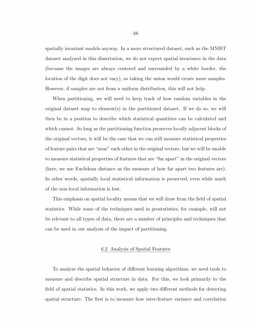
88
spatially invariant models anyway. In a more structured dataset, such as the MNIST
dataset analyzed in this dissertation, we do not expect spatial invariance in the data
(because the images are always centered and surrounded by a white border, the
location of the digit does not vary), so taking the union would create more samples.
However, if samples are not from a uniform distribution, this will not help.
When partitioning, we will need to keep track of how random variables in the
original dataset map to element(s) in the partitioned dataset. If we do so, we will
then be in a position to describe which statistical quantities can be calculated and
which cannot. So long as the partitioning function preserves locally adjacent blocks of
the original vectors, it will be the case that we can still measure statistical properties
of feature pairs that are “near” each other in the original vectors, but we will be unable
to measure statistical properties of features that are “far apart” in the original vectors
(here, we use Euclidean distance as the measure of how far apart two features are).
In other words, spatially local statistical information is preserved, even while much
of the non-local information is lost.
This emphasis on spatial locality means that we will draw from the field of spatial
statistics. While some of the techniques used in geostatistics, for example, will not
be relevant to all types of data, there are a number of principles and techniques that
can be used in our analysis of the impact of partitioning.
6.2 Analysis of Spatial Features
To analyze the spatial behavior of different learning algorithms, we need tools to
measure and describe spatial structure in data. For this, we look primarily to the
field of spatial statistics. In this work, we apply two different methods for detecting
spatial structure. The first is to measure how inter-feature variance and correlation
89
changes with spatial distance between features. This gives us a quantitative measure,
but tells us only about pair-wise relationships on average. The second is a more
holistic qualitative analysis that can be done by using dimensionality reduction to
embed the data in a plane so it can be visualized. In this way, we can find what
kind of clusters or structure exists in the data and compare the amount of structure
present in different datasets.
For quantitative analysis, we use a tool from spatial statistics called a variogram,
which lets us examine the relationship between spatial distance and statistical corre-
lation. Note again that we use spatial in the sense of spatial statistics; the distances
here are between features, not between datapoints.
The generic equation for a variogram is described in Section 2.5 as:
2γ(h) = var(Z(s+ h)− Z(s)), h ∈ Rd
where Z(s) : s ∈ D ⊂ Rd is a random process which produces n data samples
Z(s1), Z(s2), ..., Z(sn) and h is separation (distance) vector. Generally, this function
will be plotted and examined to observe the relationship between distance and dif-
ference. In geostatistics where variograms are used for predictive modeling, these
assumptions are often closely matched by the underlying problems. Here, we use an
empirical estimation of the variogram as a descriptive analytic tool. We acknowledge
that the assumptions are violated by natural image data, so a “true” variogram is not
well defined. Instead, we calculate an “average” empirical variogram. A “sample”
in the context of image analysis is basically a pixel, so the location of the sample is
merely the pixel location, and the value of the sample is the pixel value.
To generate the variogram plots, we compute the variance of each pair of features
(computed across all images in the set). For each pair of features (i.e. pixels) (i, j),
90
Figure 6.1: Variogram and mean-correlation plots for the MNIST.
we have n samples (one per image in the dataset); this can be thought of as two
vectors of values, where the length of the vector is n. We take the difference between
these vectors, and then compute the variance of the resulting vector, var(X i −Xj).
This gives us one scalar term for each pair of features. At this point, to make the
distance-based function static and isotropic, we average together all feature pairs with
equal inter-feature distances. Figure 6.1 shows the variogram and mean-correlation
of the original MNIST dataset; note that artifact at the far right side of the plots is
caused by the white “border pixels” that are an artifact of MNIST.
91
In fact, we can make similar plots for any other pairwise statistical measure; for
example, we have done something similar using correlation in place of variance-of-
differences.
6.3 Experimental Setup
Here we again used the MNIST dataset for our experiments, due to its wide use
in evaluating RBMs and deep learning algorithms. A description of the dataset is
given in Section 4.4.
We measured the performance of the DBNs using reconstruction error, which is
defined to be the mean difference between the original and reconstructed images. We
used a binary reconstruction error with a fixed threshold value of 30 to map pixels in
the range [0− 255] to a binary 1 or 0 for the original images. To get the reconstructed
image from the DBN, we propagate the image all the way to the last hidden layer of
Deep Belief Network, then reconstruct it by reverse propagation to the visible layer.
The resulting vector is binarized and compared with the original vector to calculate
a reconstruction error using following equation:
E(x,x′) =1
n
n∑i=1
I(xi 6= x′i)
To examine whether spatially local features are being preserved, we constructed
a 2-layer deep belief network, where each layer is composed of 784 hidden nodes. We
calculated the variogram and mean-correlation plot for the output of hidden nodes
at each layer.
To apply t-SNE to hidden nodes, we generated sample points by setting a se-
lected hidden neuron to 1.0 and all other hidden nodes to 0, and then computing
92
corresponding input node activations. Thus, the weights between that hidden node
to all visible nodes captures a “feature” (this can also be referred to as a filter, or
template, depending on context).
6.4 Results
To examine what statistical information is being exploited by the Partitioned-
RBMs, we performed a series of experiments on a randomly permuted version of the
data set. Since permuting the data will destroy spatially local features, this allows
us to asses how a learning model makes use of these features. To generate this new
data set, a mapping was defined that assigned each element of an input vector to
each element of the output vector with equal probability. The resultant mapping is
1-to-1 and onto, and is referred to as a random permutation. While the generation
of the mapping is randomized, once a permutation has been generated its operation
on input vectors is deterministic.
The permutation experiments were performed by generating a random partitioning
of data, applying it to each vector in the original dataset to generate a permuted
dataset, and then training the RBMs on this dataset. We can then compare the
performance of the RBMs using raw and permuted data to see whether or not the
RBMs make use of any statistical information that is disrupted by the permutation.
See the last row of Figure 6.2 for example permuted images. The last row shows the
randomly permuted images corresponding with the original images in the first row.
We also generated a variogram and a mean correlation plot for both the original
dataset and the permuted dataset to determine the presence and strength of local
statistical structure in the two versions of the dataset.
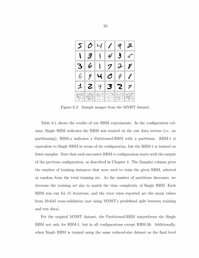
93
Figure 6.2: Sample images from the MNIST dataset.
Table 6.1 shows the results of our RBM experiments. In the configuration col-
umn, Single RBM indicates the RBM was trained on the raw data vectors (i.e. no
partitioning); RBM-n indicates a Partitioned-RBM with n partitions. RBM-1 is
equivalent to Single RBM in terms of its configuration, but the RBM-1 is trained on
fewer samples. Note that each successive RBM-n configuration starts with the output
of the previous configuration, as described in Chapter 4. The Samples column gives
the number of training instances that were used to train the given RBM, selected
at random from the total training set. As the number of partitions decreases, we
decrease the training set size to match the time complexity of Single RBM. Each
RBM was run for 15 iterations, and the error rates reported are the mean values
from 10-fold cross-validation (not using MNIST’s predefined split between training
and test data).
For the original MNIST dataset, the Partitioned-RBM outperforms the Single
RBM not only for RBM-1, but in all configurations except RBM-28. Additionally,
when Single RBM is trained using the same reduced-size dataset as the final level
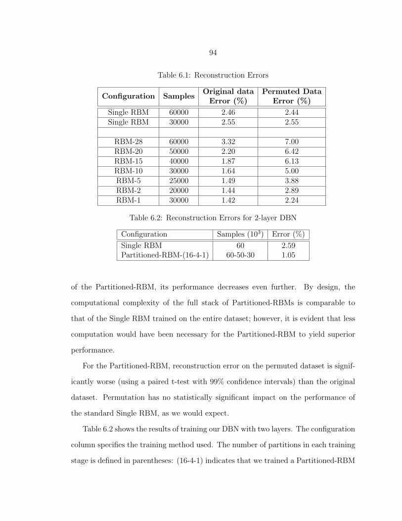
94
Table 6.1: Reconstruction Errors
Configuration SamplesOriginal data
Error (%)Permuted Data
Error (%)
Single RBM 60000 2.46 2.44Single RBM 30000 2.55 2.55
RBM-28 60000 3.32 7.00RBM-20 50000 2.20 6.42RBM-15 40000 1.87 6.13RBM-10 30000 1.64 5.00RBM-5 25000 1.49 3.88RBM-2 20000 1.44 2.89RBM-1 30000 1.42 2.24
Table 6.2: Reconstruction Errors for 2-layer DBN
Configuration Samples (103) Error (%)
Single RBM 60 2.59Partitioned-RBM-(16-4-1) 60-50-30 1.05
of the Partitioned-RBM, its performance decreases even further. By design, the
computational complexity of the full stack of Partitioned-RBMs is comparable to
that of the Single RBM trained on the entire dataset; however, it is evident that less
computation would have been necessary for the Partitioned-RBM to yield superior
performance.
For the Partitioned-RBM, reconstruction error on the permuted dataset is signif-
icantly worse (using a paired t-test with 99% confidence intervals) than the original
dataset. Permutation has no statistically significant impact on the performance of
the standard Single RBM, as we would expect.
Table 6.2 shows the results of training our DBN with two layers. The configuration
column specifies the training method used. The number of partitions in each training
stage is defined in parentheses: (16-4-1) indicates that we trained a Partitioned-RBM
95
first with 16 splits, then 4, and finally trained as a single partition. As before, when
the number of partitions decreases, we decrease the training set size to match the time
complexity of the full Partitioned-RBM training process to that of the Single RBM.
Each RBM was run for 15 iterations, and the error rates reported are the mean values
from 10-fold cross-validation (not using MNIST’s predefined split between training
and test data).
Partitioned-RBM significantly outperforms the Single RBM (p > 99.99% us-
ing a paired t-test). By design, the computational complexity of the full stack of
Partitioned-RBMs is comparable to or faster than that of the Single RBM trained
on the entire dataset; however, it is evident that less computation would have been
necessary for the Partitioned-RBM to yield superior performance.
We generated variogram and mean correlation plots as described in Section 6.2.
Figure 6.3 shows the variogram plots for subsets of the data corresponding to digits
0, 5 and 9 (from top to bottom). The first column shows variograms of the raw input
vectors for each subset, the second column shows results of the Single RBM, and
the third shows results of the Partitioned-RBM. The y−axis represents the mean
variance of differences, and the x−axis represents Euclidean pixel distance between
points. Labels of the form N−P indicate data for hidden layer N of a Deep Belief Net-
work based on Partitioned-RBMs with P partitions. For all digits, Partitioned-RBM
produces an “arch” pattern consistent with the original digit plot. In comparison,
the hidden layers of the traditional RBM do not preserve the relationship between
distance and difference. Variograms for other digits can be found in Appendix A.
Similar to variogram, Figure 6.4 shows the mean correlation plots for subsets of
the data corresponding to digits 0, 5 and 9. As with variograms, the first column
depicts digits, the second column shows results of the Single RBM, and the third
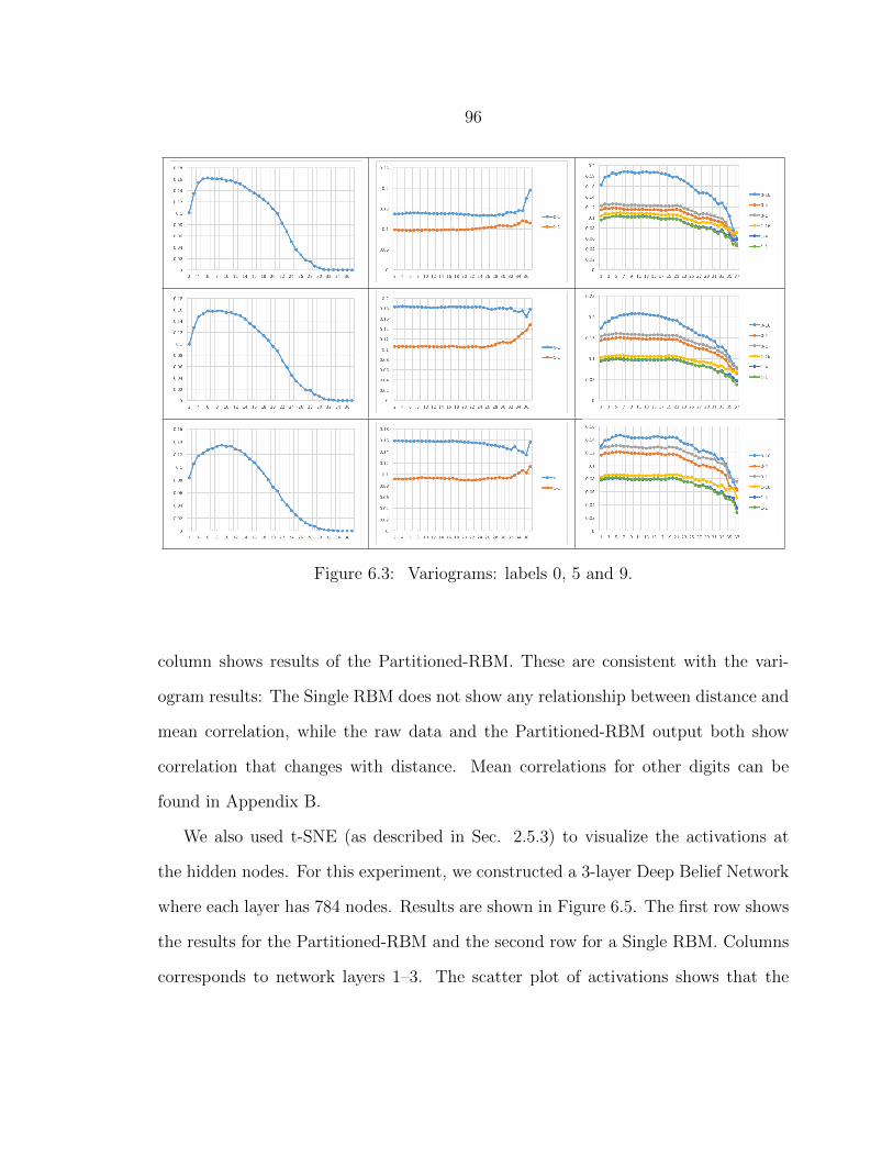
96
Figure 6.3: Variograms: labels 0, 5 and 9.
column shows results of the Partitioned-RBM. These are consistent with the vari-
ogram results: The Single RBM does not show any relationship between distance and
mean correlation, while the raw data and the Partitioned-RBM output both show
correlation that changes with distance. Mean correlations for other digits can be
found in Appendix B.
We also used t-SNE (as described in Sec. 2.5.3) to visualize the activations at
the hidden nodes. For this experiment, we constructed a 3-layer Deep Belief Network
where each layer has 784 nodes. Results are shown in Figure 6.5. The first row shows
the results for the Partitioned-RBM and the second row for a Single RBM. Columns
corresponds to network layers 1–3. The scatter plot of activations shows that the
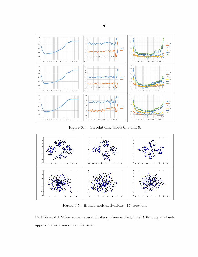
97
Figure 6.4: Correlations: labels 0, 5 and 9.
Figure 6.5: Hidden node activations: 15 iterations
Partitioned-RBM has some natural clusters, whereas the Single RBM output closely
approximates a zero-mean Gaussian.
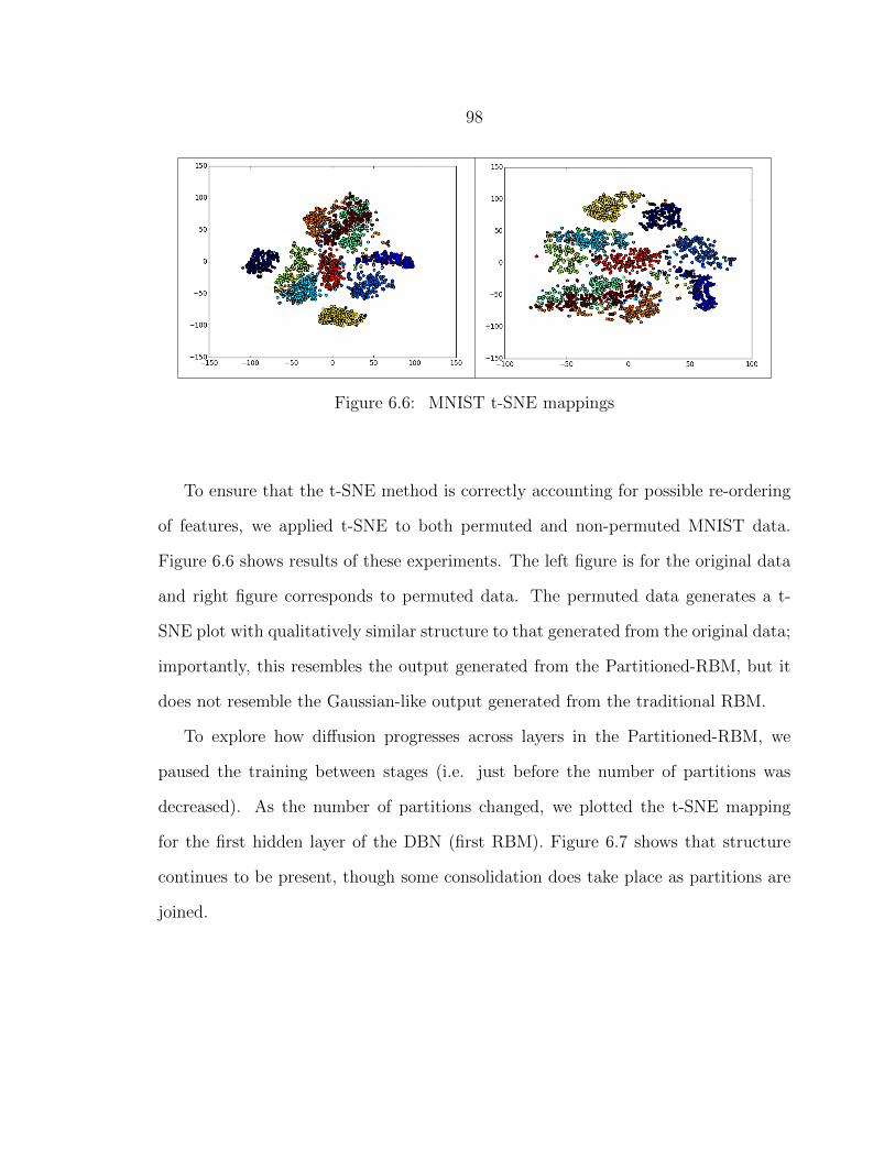
98
Figure 6.6: MNIST t-SNE mappings
To ensure that the t-SNE method is correctly accounting for possible re-ordering
of features, we applied t-SNE to both permuted and non-permuted MNIST data.
Figure 6.6 shows results of these experiments. The left figure is for the original data
and right figure corresponds to permuted data. The permuted data generates a t-
SNE plot with qualitatively similar structure to that generated from the original data;
importantly, this resembles the output generated from the Partitioned-RBM, but it
does not resemble the Gaussian-like output generated from the traditional RBM.
To explore how diffusion progresses across layers in the Partitioned-RBM, we
paused the training between stages (i.e. just before the number of partitions was
decreased). As the number of partitions changed, we plotted the t-SNE mapping
for the first hidden layer of the DBN (first RBM). Figure 6.7 shows that structure
continues to be present, though some consolidation does take place as partitions are
joined.
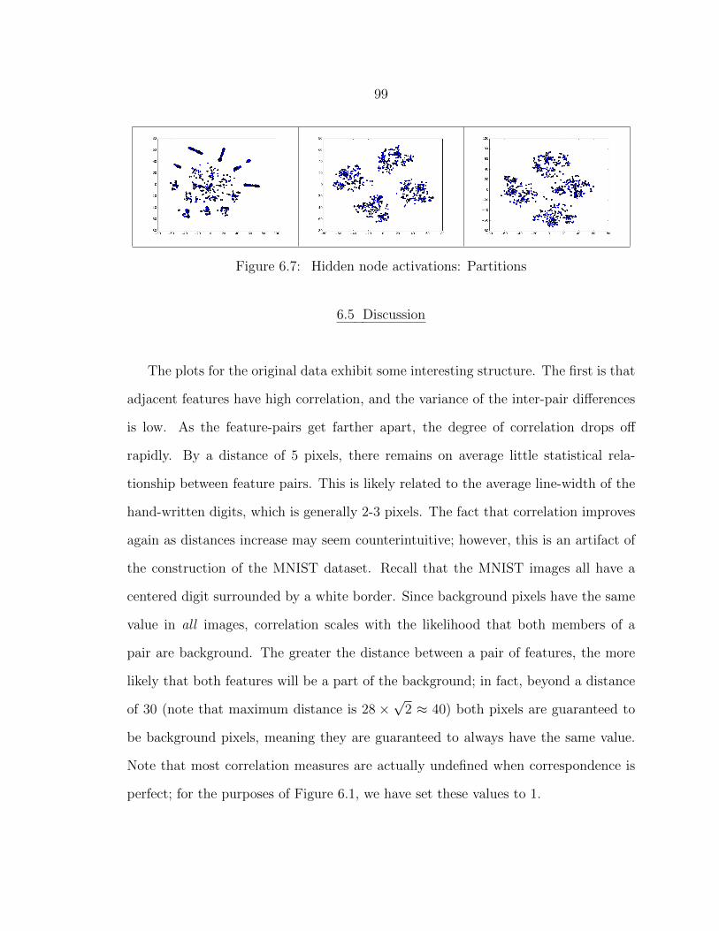
99
Figure 6.7: Hidden node activations: Partitions
6.5 Discussion
The plots for the original data exhibit some interesting structure. The first is that
adjacent features have high correlation, and the variance of the inter-pair differences
is low. As the feature-pairs get farther apart, the degree of correlation drops off
rapidly. By a distance of 5 pixels, there remains on average little statistical rela-
tionship between feature pairs. This is likely related to the average line-width of the
hand-written digits, which is generally 2-3 pixels. The fact that correlation improves
again as distances increase may seem counterintuitive; however, this is an artifact of
the construction of the MNIST dataset. Recall that the MNIST images all have a
centered digit surrounded by a white border. Since background pixels have the same
value in all images, correlation scales with the likelihood that both members of a
pair are background. The greater the distance between a pair of features, the more
likely that both features will be a part of the background; in fact, beyond a distance
of 30 (note that maximum distance is 28 ×√
2 ≈ 40) both pixels are guaranteed to
be background pixels, meaning they are guaranteed to always have the same value.
Note that most correlation measures are actually undefined when correspondence is
perfect; for the purposes of Figure 6.1, we have set these values to 1.
100
From the results of our experiments using the permuted dataset, we believe that
the Partitioned-RBM is making use of statistical information that is spatially local-
ized, where the Single RBM is not. The permutation results in no loss of information
for the Single RBM. It simply re-orders the elements of the vectors. For this reason,
any pair-wise correlation between a given pair of features will be unaltered by the
permutation. The unchanged behavior of the Single RBM is, therefore, exactly what
we expected.
Things are different for the Partitioned-RBM, however, since the location of the
two features in a given pair will be altered. This means that two features that would
have been assigned to the same partition in the original dataset might not be assigned
to the same partition in the permuted dataset. Since each piece of a Partitioned-
RBM only has access to features in its partition, this means that whatever statistical
information was contained in the correlation between this pair of features is no longer
available to the Partitioned-RBM.
In fact, Partitioned-RBM will always be cut off from a great many of the pair-
wise feature correlations; the difference between the original and permuted datasets
is simply in which correlations are lost. The fact that the Partitioned-RBM performs
significantly worse on the permuted dataset implies that not all correlations are of
equal value. In particular, it means that correlations between pairs of features that are
spatially close in the original data are more important to the success of the algorithm
than correlations between arbitrary pairs (which will, on average, be significantly
farther apart in the original image).
Thus, the results lead us readily to the conclusion that the Partitioned-RBM is
making use of spatially local statistical information in the MNIST dataset to achieve
its performance. Work described [35] that partitioned deep learning algorithms rely
on such local information.
101
We have begun to explore one of the potential representation biases that deep
learning techniques leverage to achieve their performance. Our experimental results
suggest that partitioned-data techniques are able to make use of spatially local in-
formation, and we have in the variogram and the mean-correlation plot some crude
tools for analyzing how much spatially local structure exists in a dataset. While these
results are promising, they offer only a first jumping off point for the work that could
be done in the area of understanding and exploiting the biases that underpin deep
learning.
In partitioned learning models, the partitioning can be thought of as a simplify-
ing assumption that reduces both the total number of parameters and the number
of inter-parameter dependencies, thus simplifying the learning process. If the data
conform to this assumption, this should provide an advantage. We have tested the
validity of this assumption by training partitioned models on both “normal” images
and “scrambled” images (in which spatially a local structure was intentionally de-
stroyed by permutation, but no statistical information was lost if the full vectors
were considered). As expected, if the data badly violates the assumption of spa-
tially local patterns, performance of partitioning techniques is severely degraded, but
performance on non-scrambled images is increased by using partitioning [35].
One problem with these results is that they do not cover all deep learning meth-
ods; DBNs, for example, do not normally take a partitioned approach, so there may
be different principles at play in their success. We mainly focused on the question
of whether DBNs are in fact making use of spatially local statistical information,
and if not whether we can modify the training procedure to incorporate this spatial
locality prior and improve the performance of the network (without modifying the
overall architecture or operation of the final DBN model). From the results of our
experiments using spatial statistics and t-SNE, we conclude that the Partitioned-
102
RBM in a Deep Belief Network is making use of spatially local information, where
the Single RBM-based DBN is not. The variograms (Fig. 6.3) demonstrate that the
Partitioned-RBM output has broadly similar spatial statistics as the original dataset.
While the plots are not identical, similar overall trends are present. Partitioned-RBM
training preserves these statistical patterns even in higher layers of the network. The
same plots for Single RBM training show that spatial locality is lost in the first hidden
layer.
Figure 6.6 shows what happens when the original data is scrambled beforehand, by
generating a random permutation, and then applying it to each input vector. Despite
the disruption of spatial organization of features, the transformation is lossless, and
structure obtained in the t-SNE projection is similar to that for the original data.
This suggests that if the Single RBM had preserved any spatial features, we should
see similar structure in the t-SNE projection (even if the spatial organization of those
features was not preserved). As the t-SNE results show, there is no structure in the
t-SNE projection after the first layer of the Single RBM; the projected distribution
closely approximates a Gaussian (i.e., it is indistinguishable from noise). Thus, we
conclude that the traditional RBMs do not retain spatially local statistical informa-
tion in any recoverable form. As a result, any deep network trained using standard
RBMs will lose all spatial information in the first hidden layer. On the other hand, the
Partitioned-RBM training technique preserves spatially local information, meaning a
deep network trained using this method can make use of spatial patterns in all layers
of the network.
This result, combined with the performance edge the Partitioned-RBM has in
practice, reinforces the hypothesis that the MNIST data has relevant spatially lo-
cal structure, and that like other partitioned deep methods, the Partitioned-RBM
achieves its performance due to an implicit model bias that assumes (and exploits) the
103
presence of spatially local features. DBNs trained with the standard RBM method
lose spatially local features, and are therefore at a disadvantage because they are
attempting to solve a harder problem. Without the constraint imposed by the as-
sumption of local structure, the standard RBM training algorithm is left with a much
larger hypothesis space to search.
104
CHAPTER 7
TIME SERIES CLASSIFICATION VIA PARTITIONED NETWORKS
Since time series data are typically very high dimensional, the use of RBMs in
time series tasks is not common. But, in recent years, there have been a few attempts
to use RBMs in high dimensional data such as time series and motion data. The
following sections summarizes these studies. In the rest of this chapter, we describe
Temporal Partitioned Restricted Boltzmann Machines (TPRBM), using partitioned-
based training. We apply our partitioned model and Dynamic Time Warping (DTW)
to several time series datasets for a sequence classification task.
7.1 Time Series Classification
We begin with a definition of time series data type.
Definition 7.1.1. (Time Series) T = t1, . . . , tn is an ordered set of n real-valued
variables.
Depending on classification task, some times we are interested in the classifying
the whole time series and sometimes a subsequence of the dataset. However, often the
whole time series is not informative. For instance, four hours recording of a patient’s
heartbeat may not tell us if the hearbeat is abnormal or not. But, a subsequence of
dataset may contain an abnormal pattern.
Definition 7.1.2. (Subsequence) Given a time series T of length n, a subsequence
Ts = ts, . . . , ts + w where w < n is the length of subsection.
105
In addition to DTW scoring method described in Section 2.5.4, Euclidean Distance
is one of the most common measure for clasification.
Definition 7.1.3. (Euclidean Distance) Given two time series T and S with both of
length n, Euclidean distance is the square root of the sum of the squared differences
between each pair of time values:
d(T, S) =
√√√√ n∑n=1
(ti − si)2
Time series prediction is a process of finding the value of ti for given previous
t1, . . . , tj−1 values. Time series classification on the other hand, involves finding a
categorical label for a giving time series. Classification is a specifically useful tool for
indexing and querying a database of time series.
Definition 7.1.4. (Time Series Classification) Given a set of unlabeled time series,
the task of time series classification is assign a label from one of the predefined classes.
A considerable amount of literature has been published on time series prediction
and classification. In fact, time series prediction has been studied in statistics over
many decades. One of the most successful models, Autoregressive Moving Average
(ARMA), was developed by Peter Whittle in 1951 [76] and popularized by George E.
P. Box and Gwilym Jenkins in 1971 [77]. ARMA and its extension, Autoregressive
Integrated Moving Average (ARIMA), are still very popular time series prediction
models today. It has only been over the last couple of decades that machine learning
has been used for time series prediction tasks using methods such as Neural Networks
and Support Vector Machines.
On the other hand, the need for time series classification mainly has arisen when
people need to store/index large volumes of time series data and query that. For
106
example, querying a gene sequence database for given sequence pattern requires clas-
sification. Dynamic Time Warping (DTW), discussed in Chapter 2, is one of the most
important tools for time series classification.
7.2 Temporal Restricted Boltzmann Machines
The Conditional Restricted Boltzmann Machine (CRBM) is a non-linear genera-
tive model designed to model human motion where real-valued visible variables repre-
sent joint angles and hidden/latent variables represents motion [78]. The model is the
same as a regular RBM; however, the hidden and visible layers are both conditioned
on visible variables from the last few time-steps.
As shown in Figure 7.1a, the hidden layer and visible layer both have direct
connections from the visible layer in previous time steps. Given data at n previous
steps, hidden layers are independent. With a minor change to the energy function,
the Contrastive Divergence algorithm is used for training CRBMs. The only change
required is to use direct connections from previous layers to update hidden and visible
biases. For a regular RBM, the energy function is the following:
E(x,h) = −hTWx− bTx− cTh,
whereas the CRBMs, the energy function becomes:
E(x,u,h) = −hTWx− bTx− cTh− uTWx− uTWh
where u is an input vector that represents a visible layer from the previous time step.
So, the only change is including components with the u term.
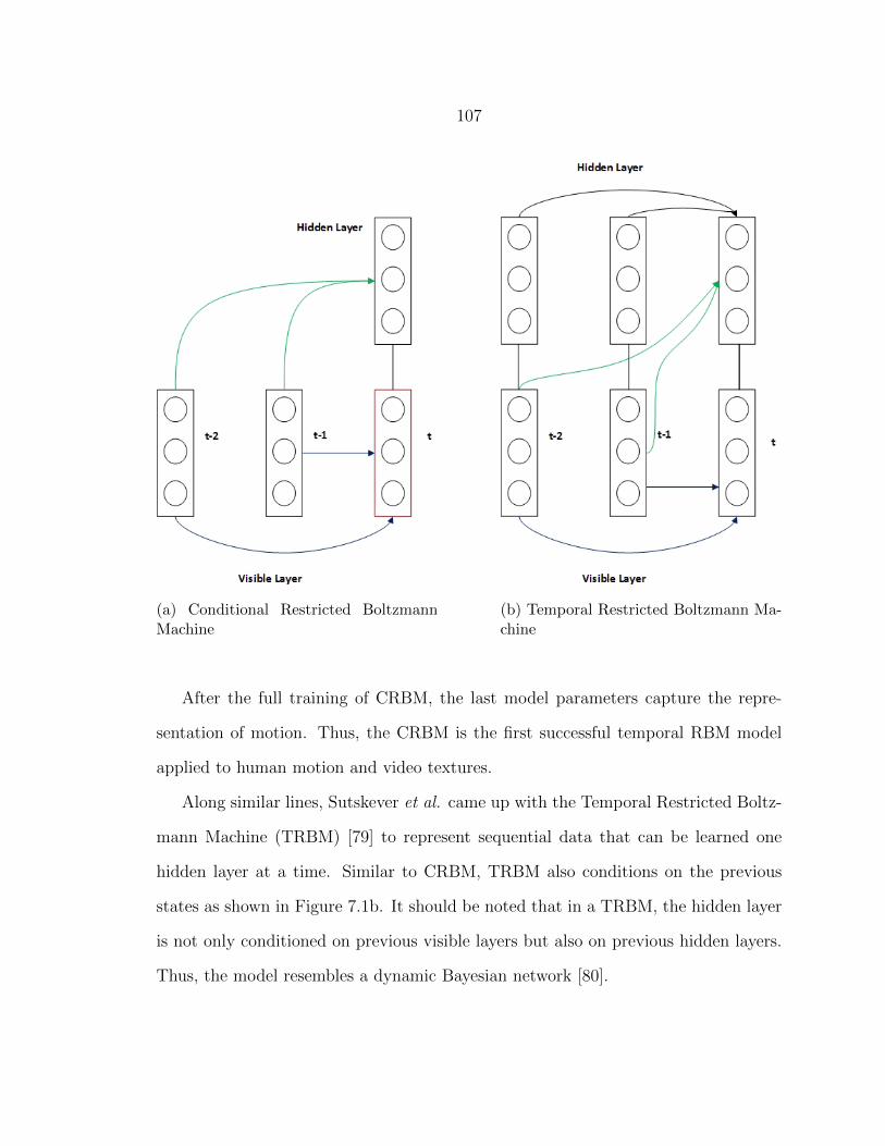
107
(a) Conditional Restricted BoltzmannMachine
(b) Temporal Restricted Boltzmann Ma-chine
After the full training of CRBM, the last model parameters capture the repre-
sentation of motion. Thus, the CRBM is the first successful temporal RBM model
applied to human motion and video textures.
Along similar lines, Sutskever et al. came up with the Temporal Restricted Boltz-
mann Machine (TRBM) [79] to represent sequential data that can be learned one
hidden layer at a time. Similar to CRBM, TRBM also conditions on the previous
states as shown in Figure 7.1b. It should be noted that in a TRBM, the hidden layer
is not only conditioned on previous visible layers but also on previous hidden layers.
Thus, the model resembles a dynamic Bayesian network [80].
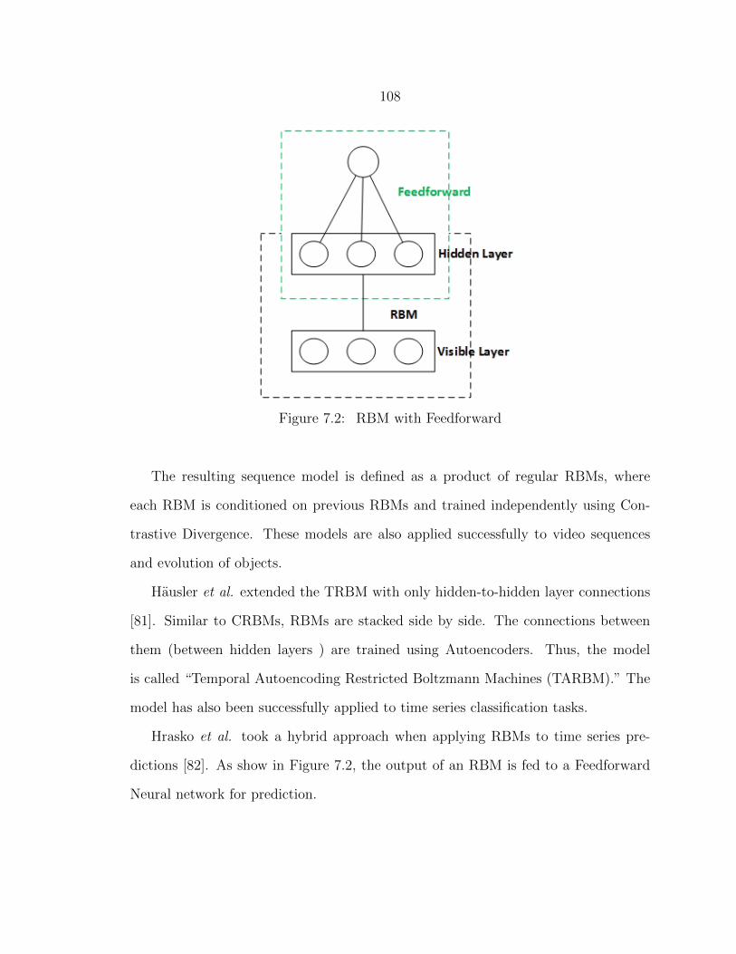
108
Figure 7.2: RBM with Feedforward
The resulting sequence model is defined as a product of regular RBMs, where
each RBM is conditioned on previous RBMs and trained independently using Con-
trastive Divergence. These models are also applied successfully to video sequences
and evolution of objects.
Hausler et al. extended the TRBM with only hidden-to-hidden layer connections
[81]. Similar to CRBMs, RBMs are stacked side by side. The connections between
them (between hidden layers ) are trained using Autoencoders. Thus, the model
is called “Temporal Autoencoding Restricted Boltzmann Machines (TARBM).” The
model has also been successfully applied to time series classification tasks.
Hrasko et al. took a hybrid approach when applying RBMs to time series pre-
dictions [82]. As show in Figure 7.2, the output of an RBM is fed to a Feedforward
Neural network for prediction.
109
7.3 Partitioned Restricted Boltzmann Machines
Here, we show that Partitioned-RBM is a natural model for learning time series
classification for the following reasons. 1) Each partition can learn local features or
trends efficiently since sub-RBMs are small. 2) As we combine partitions, at the
later stages of the learning, the model can learn longer trends and features. 3) Time
series have very high dimensions; thus, by partitioning the data as well as the model,
Partitioned-RBM will significantly improve the computational performance.
TPRBM is basically the same model as Partitioned-RBM described in Chapter
5. However, instead of using quadtree partitioning, here we use a naıve partitioning.
The whole time series is divided into k sub-vectors without overlap. The remainder
of the training is the same. For example, Figure 7.3 represents a time series of length
132 and four partitions. Each RBM works on one section of the time series.
The idea here is that each individual RBM will capture local trends/features
within the window. Thus, distant features will not be represented. However, in
later stages, when we have fewer splits, distant features will also be captured. We
demonstrated in Chapter 6 that regular RBMs do not preserve spatially local features.
We assert that regular RBMs will not preserve temporal local trends and features
either. Moreover, as demonstrated by Schulz et al., a monolithic RBM will not
capture local features as most of its detectors will have uniform weights after the
training is done [56].
Training time complexities of regular RBMs and Partitioned-RBMs are given in
Equations 4.1 and 4.2, which are repeated here for convenience. The time complexity
of regular RBM is O(I · S · H · V ) where I, S, H, and V are number of iterations,
number of samples, number of hidden nodes, and number of visible nodes respectively.
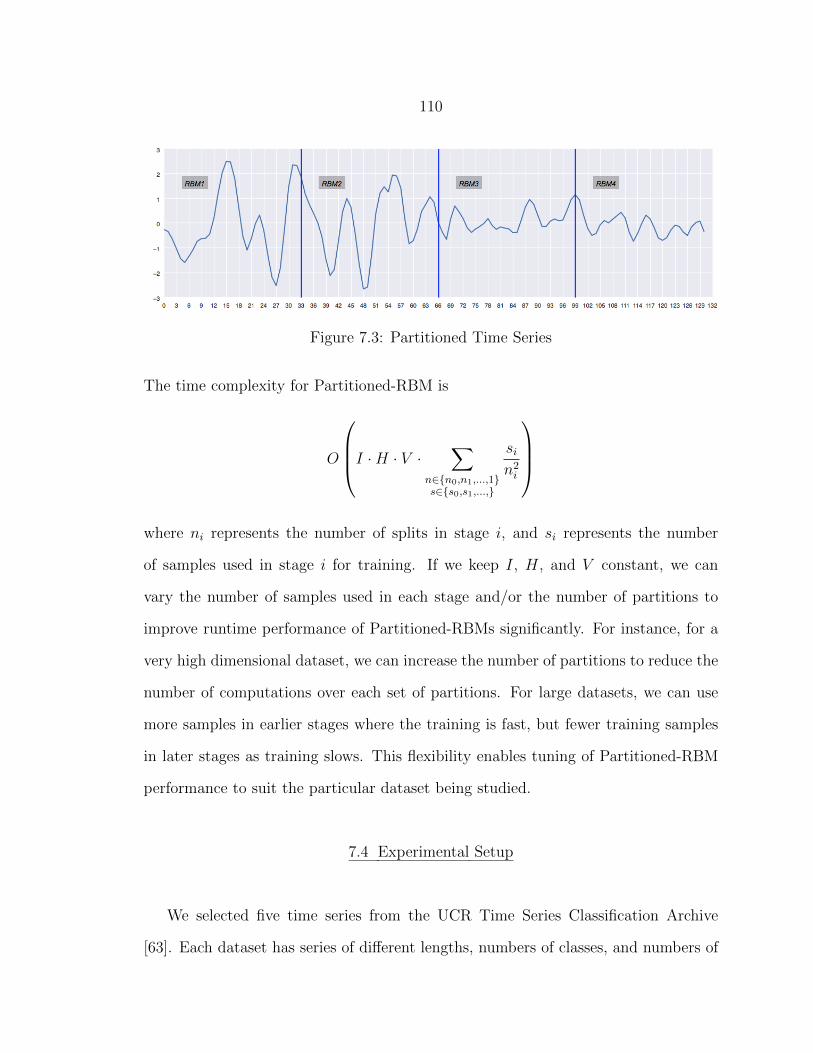
110
Figure 7.3: Partitioned Time Series
The time complexity for Partitioned-RBM is
O
I ·H · V · ∑n∈n0,n1,...,1s∈s0,s1,...,
sin2i
where ni represents the number of splits in stage i, and si represents the number
of samples used in stage i for training. If we keep I, H, and V constant, we can
vary the number of samples used in each stage and/or the number of partitions to
improve runtime performance of Partitioned-RBMs significantly. For instance, for a
very high dimensional dataset, we can increase the number of partitions to reduce the
number of computations over each set of partitions. For large datasets, we can use
more samples in earlier stages where the training is fast, but fewer training samples
in later stages as training slows. This flexibility enables tuning of Partitioned-RBM
performance to suit the particular dataset being studied.
7.4 Experimental Setup
We selected five time series from the UCR Time Series Classification Archive
[63]. Each dataset has series of different lengths, numbers of classes, and numbers of
111
Table 7.1: Partitioned-RBM configuration
DataSeries
Size Labels Samples PartitionsHiddennodes
FaceAll 131 14 2250 50-20-5-1 1000RefrigerationDevices 720 3 750 50-20-5-1 1000ECG5000 140 5 5000 50-20-5-1 1000ElectricDevices 96 7 16637 20-5-1 1000ShapesAll 512 60 1200 50-20-5-1 1000
samples. The UCR time series are split into test and training sets. Generally, the
training set is a lot smaller than the test set because prior studies mostly used the k-
Nearest-Neighbor algorithm for classification (k-NN). k-Nearest-Neighbor Classifiers
is a lazy learner [83]; the model is constructed during query or classification time. In
query time, however, using a large training set is inefficient. Thus, we did not use
the pre-defined test and training batches. Instead, we combined both to create a full
dataset so that we could use 10-fold cross-validation. Moreover, we binarized data
using the following naıve method: anything less than or equal to 0 was set 0 and
anything greater than 0 was set to 1.
The time series datasets that we used are shown in Table 7.1. The size column
indicates the time series length, and the partitions column indicates the number of
partitions used to train Partitioned-RBM. 50−20−5−1 means, we initially trained the
model with 50 partitions followed by 20 partitions in the second stage, and 5 partitions
in third. In the final stage, we trained the model as a full RBM. It should be noted,
however, that we selected samples in each stage such that the time complexity of
Partitioned-RBM is comparable to or better than that of Single RBM.
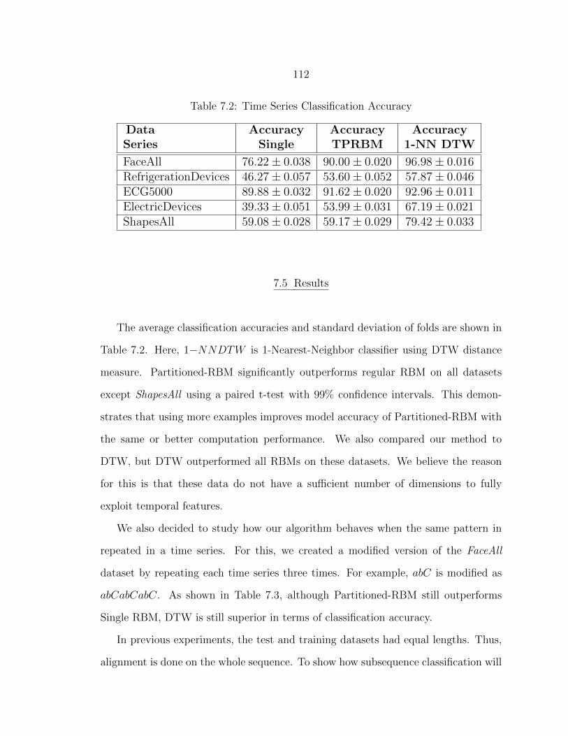
112
Table 7.2: Time Series Classification Accuracy
DataSeries
AccuracySingle
AccuracyTPRBM
Accuracy1-NN DTW
FaceAll 76.22± 0.038 90.00± 0.020 96.98± 0.016RefrigerationDevices 46.27± 0.057 53.60± 0.052 57.87± 0.046ECG5000 89.88± 0.032 91.62± 0.020 92.96± 0.011ElectricDevices 39.33± 0.051 53.99± 0.031 67.19± 0.021ShapesAll 59.08± 0.028 59.17± 0.029 79.42± 0.033
7.5 Results
The average classification accuracies and standard deviation of folds are shown in
Table 7.2. Here, 1−NNDTW is 1-Nearest-Neighbor classifier using DTW distance
measure. Partitioned-RBM significantly outperforms regular RBM on all datasets
except ShapesAll using a paired t-test with 99% confidence intervals. This demon-
strates that using more examples improves model accuracy of Partitioned-RBM with
the same or better computation performance. We also compared our method to
DTW, but DTW outperformed all RBMs on these datasets. We believe the reason
for this is that these data do not have a sufficient number of dimensions to fully
exploit temporal features.
We also decided to study how our algorithm behaves when the same pattern in
repeated in a time series. For this, we created a modified version of the FaceAll
dataset by repeating each time series three times. For example, abC is modified as
abCabCabC. As shown in Table 7.3, although Partitioned-RBM still outperforms
Single RBM, DTW is still superior in terms of classification accuracy.
In previous experiments, the test and training datasets had equal lengths. Thus,
alignment is done on the whole sequence. To show how subsequence classification will
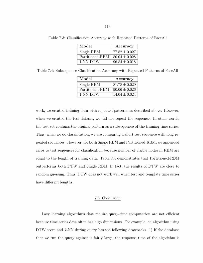
113
Table 7.3: Classification Accuracy with Repeated Patterns of FaceAll
Model Accuracy
Single RBM 77.82± 0.027Partitioned-RBM 80.04± 0.0281-NN DTW 96.84± 0.018
Table 7.4: Subsequence Classification Accuracy with Repeated Patterns of FaceAll
Model Accuracy
Single RBM 81.78± 0.029Partitioned-RBM 90.06± 0.0261-NN DTW 14.04± 0.024
work, we created training data with repeated patterns as described above. However,
when we created the test dataset, we did not repeat the sequence. In other words,
the test set contains the original pattern as a subsequence of the training time series.
Thus, when we do classification, we are comparing a short test sequence with long re-
peated sequences. However, for both Single RBM and Partitioned-RBM, we appended
zeros to test sequences for classification because number of visible nodes in RBM are
equal to the length of training data. Table 7.4 demonstrates that Partitioned-RBM
outperforms both DTW and Single RBM. In fact, the results of DTW are close to
random guessing. Thus, DTW does not work well when test and template time series
have different lengths.
7.6 Conclusion
Lazy learning algorithms that require query-time computation are not efficient
because time series data often has high dimensions. For example, an algorithm using
DTW score and k-NN during query has the following drawbacks. 1) If the database
that we run the query against is fairly large, the response time of the algorithm is
114
very slow. 2) Because of the first drawback, one has to select a subset of the dataset
for runtime query; however, this kind of knowledge engineering is expensive. We
selected samples in each stage such that the time complexity of Partitioned-RBM
is comparable to or better than that of Single RBM. Thus, we demonstrated that
Partitioned-RBM can effectively be applied to time series datasets without these
drawbacks.
115
CHAPTER 8
SUMMARY AND CONCLUSIONS
In this dissertation, we presented a partitioned learning approach and applied it
to Restricted Boltzmann Machines. Specifically, we demonstrated the effectiveness of
this method in the context of both standalone RBMs and DBNs. In this chapter, we
conclude with a summary of our contributions and directions for future work.
8.1 Summary of Contributions
8.1.1 Partitioned Learning
This study set out to develop a generic learning algorithm that not only partitions
the input vector, but also the model parameters. Thus, we developed a novel meta-
algorithm that converts a monolithic model into submodels where each submodel is
trained on a corresponding partition of the input vector. However, learning proceeds
in multiple stages where the model and the input vector are split into fewer partitions
in each successive stage. In other words, as the stages proceed, smaller partitions are
combined into larger partitions. This dissertation has shown that this partitioned
approach results in better feature representation.
8.1.2 Computational Efficiency
As we demonstrated in Chapter 4, training Partitioned-RBMs is faster than
training non-partitioned versions. In addition, we demonstrated that Partitioned-
RBMs have the same or better feature representation power as a monolithic RBM,
116
Partitioned-RBMs yield two major improvements: 1) a faster algorithm for learn-
ing with high dimensional data; and 2) a novel algorithm for training RBMs under
resource-bounded conditions. When there are limited computational resources, the
algorithm can terminate early with a good generative performance.
8.1.3 Efficient Classification
We demonstrated in Chapter 4 that Partitioned-RBM can be used efficiently as a
discriminative model. We demonstrated that Partitioned-RBM has the same or better
classification accuracy as regular RBMs. However, it requires less computation.
8.1.4 Preserving Spatially Local Features
As shown in Chapter 6, Partitioned-RBM can be used effectively as part of Deep
Belief Networks. We further demonstrated that Partitioned-RBM preserves spatially
local features while regular RBM-based DBN does not.
8.1.5 Sparsity
A sparse RBM is a model that, when trained, has most of the weights close to zero
and only a few either highly positive or highly negative. In a sparse RBM, only a few
neurons (hidden nodes) will be active at any given time. This enables the network
to learn sparse representations. Researchers often limit the number of neurons that
are active for a given input by explicitly adding a sparsity factor in the training
process so that most of the weights between visible and hidden nodes are close to
zero. Partitioned-RBMs possess natural sparsity because each Partitioned-RBM is
trained on a reduced region of the dataset.
117
8.1.6 Time Series Classification
In Chapter 7, we demonstrated that Partitioned-RBMs are effective in a time
series classification task. The partitioned training model fits well with time series
datasets because such datasets have very high dimensions. Both regular RBMs and
DTW-based k-Nearest Neighbor algorithms cannot perform well when the dimen-
sionality is very high. Moreover, since DTW requires query time model construction,
knowledge engineering is needed to select a subset of the whole data, making this
method impractical.
8.2 Publications
This study resulted in several published papers and more papers to be submitted
for publication. The related publications are:
• H. Tosun and J. W. Sheppard, Training restricted Boltzmann machines with
overlapping partitions, in Proceedings of the European Conference on Machine
Learning-Principles and Practice of Knowledge Discovery in Databases (ECML-
PKDD). Springer, 2014, vol. 8726, pp. 195-208.
• B. Mitchell, H. Tosun, and J. Sheppard, Deep learning using partitioned data
vectors, in Proceedings of the IEEE International Joint Conference on Neural
Networks (IJCNN), 2015, pp. 1–8.
• H. Tosun, B. Mitchell, and J. Sheppard, Assessing diffusion of spatial features
in deep belief networks, to appear in IEEE International Joint Conference on
Neural Networks (IJCNN), 2016.
118
• H. Tosun and J. Sheppard, Fast classification under bounded computational
resources using partitioned-rbms, to appear in IEEE International Joint Con-
ference on Neural Networks (IJCNN), 2016.
• H. Tosun and J. Sheppard, Fast time series classification using Partitioned Re-
stricted Boltzmann Machines, conference or journal to be identified.
8.3 Future Work
Our approach opens the door to many potential applications. Since training is
done on partitioned small RBMs, we believe the method will learn multi-mode data,
that is data from multiple sources, more accurately. Other directions for future work
include carrying out additional experiments to demonstrate that this training method
can be applied to domains with a high volume of features.
Our algorithm also has similarities to transfer learning. Since in each stage we
learn some weights and those weights are used as a base configuration for the next
stage, it is analogous to feature representation transfer [84]. One interesting direction
for future work would be to investigate whether other methods of transfer learning
can be used during training.
In Chapter 5 we demonstrated that Partitioned-RBM performs significantly better
than single RBM under bounded computational resources. To see our method perform
even better, we need to run it on a dataset with extremely high volume and high
dimensions. We speculate that a single RBM cannot be trained optimally unless it
runs many iterations, which will take days to train. On the other hand, Partitioned-
RBM can run many iterations in the first stage with all data samples efficiently. We
119
are planning to use this scheme to run classification tasks on many datasets with high
dimensions and high volume.
Moreover, better runtime performance also enables us to create an ensemble of
Partitioned-RBMs. Therefore, we plan to run experiments using ensembles. We
hypothesize that an ensemble of Partitioned-RBMs will result in even better classifi-
cation accuracy.
The results of our classification study also suggest that Partitioned-RBM will
provide even better runtime improvement when used as a component of a DBN. As we
stack up more layers of RBMs, the runtime performance becomes more relevant. Our
preliminary experiments indicate that Partitioned-RBM has comparable classification
accuracy rates with Single RBM when used in DBNs. Contrary to expectation, the
results were not significantly better. Additionally, we found that a DBN does not
increase accuracy rates drastically as compared to a regular RBM. It is possible this
is because of the relative simplicity of the MNIST data set. Hence, we plan to 1)
explore methods to improve classification accuracy of Partitioned-RBM when used
as a component of a DBN, 2) investigate why a DBN does not drastically improve
accuracy rates, and 3) investigate alternative data sets.
As we demonstrated with DBNs, Partitioned-RBM preserves statistical spatial
features in all layers of the network, while regular RBMs diffuse all spatially local
features. We plan to carry out further experiments to determine whether preserving
statistically local features will result in higher classification accuracy.
Traditional DBNs achieve remarkable performance when applied to classification,
image recognition and many other applications. We have begun to explore applica-
tions where we can apply partitioned-data techniques, and we are in the process of
comparing a partitioned-data DBN to a traditional DBN in terms of classification
performance (as opposed to the reconstruction task examined here). This is impor-
120
tant in two ways: 1) we would like to determine whether preserving spatially local
structure in higher layers of the network can improve classification accuracy, and 2)
we would like to explore further how and why deep learning works, by analyzing how
traditional DBNs achieve their performance even without exploiting any spatially
local information.
When applied to time series classification, we demonstrated that Partitioned-RBM
outperforms regular RBMs. However, the time series in the datasets we have chosen
have relatively short lengths. Applying query-based algorithms to time series with
very long lengths will become impractical. However, with Partitioned-RBM, we can
increase the number of partitions and therefore, thereby increase the computation
performance. As a result, we should be able to obtain even better classification
accuracies.
Finally, we also plan to develop with a better Partitioned-RBM subset classifi-
cation of time series. So far, we have implemented a fairly naıve method by setting
all missing values to 0. A reasonable approach in this direction will be to have each
partition to return a classification score. In other word, each sub RBM will have
its own classification nodes. Some kind of majority-voting mechanism needs to be
applied to obtain final classification score.

121
REFERENCES CITED
122
[1] Tijmen Tieleman. Training restricted boltzmann machines using approximationsto the likelihood gradient. Proceedings of the 25th International Conference onMachine Learning, pages 1064–1071. ACM, 2008.
[2] Ooh! ahh! google images presents a nicer way to surf the visualweb [online]. Available at http://googleblog.blogspot.com/2010/07/
ooh-ahh-google-images-presents-nicer.html, Accessed 2014-08-09.
[3] Bruno A Olshausen, i in. Emergence of simple-cell receptive field properties bylearning a sparse code for natural images. Nature, 381:607–609, 1996.
[4] Yoshua Bengio, Aaron Courville, Pascal Vincent. Representation learning: A re-view and new perspectives. IEEE Transactions on Pattern Analysis and MachineIntelligence, 35:1798–1828, 2013.
[5] Hasari Tosun, John W. Sheppard. Training restricted boltzmann machineswith overlapping partitions. Machine Learning and Knowledge Discovery inDatabases,ECML PKDD, Volume 8726 series Lecture Notes in Computer Sci-ence, pages 195–208. Springer, 2014.
[6] Don S Lemons. A student’s guide to entropy. Cambridge University Press, 2013.
[7] P. Smolensky. Information processing in dynamical systems: Foundations ofharmony theory. David E. Rumelhart, James L. McClelland, editors, ParallelDistributed Processing: Explorations in the Microstructure of Cognition, Vol. 1,pages 194–281. MIT Press, Cambridge, MA, USA, 1986.
[8] David H Ackley, Geoffrey E Hinton, Terrence J Sejnowski. A learning algorithmfor boltzmann machines. Cognitive Science, 9:147–169, 1985.
[9] Geoffrey E Hinton. Training products of experts by minimizing contrastive di-vergence. Neural computation, 14:1771–1800, 2002.
[10] Yoshua Bengio. Learning deep architectures for ai. Foundations and Trends inMachine Learning, 2:1–127, 2009.
[11] Geoffrey E Hinton, Ruslan R Salakhutdinov. Reducing the dimensionality ofdata with neural networks. Science, 313:504–507, 2006.
[12] Noel A. C. Cressie. Statistics for Spatial Data. Wiley-Interscience, 1993.
[13] Alan E Gelfand, Peter Diggle, Peter Guttorp, Montserrat Fuentes. Handbook ofspatial statistics. CRC press, 2010.
[14] Michael de Smith, Michael F. Goodchild, Paul A Longley. Geospatial Analysis.The Winchelsea Press, 2015.
123
[15] Laurens Van der Maaten, Geoffrey Hinton. Visualizing data using t-sne. Journalof Machine Learning Research, 9:2579–2605, 2008.
[16] T Cox, M Cox. Multidimensional scaling. Chapman&Hall, London, UK, 1994.
[17] Lawrence K Saul, Sam T Roweis. An introduction to locally linear embedding.Available at: http://www. cs. toronto. edu/˜roweis/lle/publications.html, 2000.
[18] Hiroaki Sakoe, Seibi Chiba. Dynamic programming algorithm optimization forspoken word recognition. Acoustics, Speech and Signal Processing, IEEE Trans-actions on, 26:43–49, 1978.
[19] Max Welling, Yee W Teh. Bayesian learning via stochastic gradient langevindynamics. Proceedings of the International Conference on Machine Learning,pages 681–688, 2011.
[20] Sungjin Ahn, Anoop Korattikara, Max Welling. Bayesian posterior sampling viastochastic gradient fisher scoring. Proceedings of the International Conferenceon Machine Learning, pages 1591–1598, 2012.
[21] Lucien Le Cam. Asymptotic methods in statistical decision theory. SpringerScience & Business Media, 2012.
[22] Yoshua Bengio, Pascal Lamblin, Dan Popovici, Hugo Larochelle. Greedy layer-wise training of deep networks. Advances in Neural Information Processing Sys-tems, 19:153–160, 2007.
[23] Geoffrey Hinton, Ruslan Salakhutdinov. Discovering binary codes for documentsby learning deep generative models. Topics in Cognitive Science, 3:74–91, 2011.
[24] George E Dahl, Ryan P Adams, Hugo Larochelle. Training restricted boltzmannmachines on word observations. Proceedings of the 29th International Conferenceon Machine Learning, pages 679–686. ACM, 2012.
[25] Hugo Larochelle, Yoshua Bengio. Classification using discriminative restrictedboltzmann machines. Proceedings of the 25th International Conference on Ma-chine Learning, pages 536–543. ACM, 2008.
[26] Jerome Louradour, Hugo Larochelle. Classification of sets using restricted boltz-mann machines. Uncertainty in Artificial Intelligence, pages 463–470. AUAI,2011.
[27] Ruslan Salakhutdinov, Andriy Mnih, Geoffrey Hinton. Restricted boltzmannmachines for collaborative filtering. Proceedings of the 24th International Con-ference on Machine Learning, pages 791–798. ACM, 2007.
124
[28] Daphne Koller, Nir Friedman. Probabilistic Graphical Models: Principles andTechniques. MIT press, 2009.
[29] Philemon Brakel, Sander Dieleman, Benjamin Schrauwen. Training restrictedboltzmann machines with multi-tempering: Harnessing parallelization. ArtificialNeural Networks and Machine Learning–ICANN 2012, pages 92–99. Springer,2012.
[30] Guido Montufar, Jason Morton. Discrete restricted boltzmann machines. TheJournal of Machine Learning Research, 16:653–672, 2015.
[31] Benjamin M. Marlin, Nando de Freitas. Asymptotic efficiency of deterministicestimators for discrete energy-based models: Ratio matching and pseudolikeli-hood. CoRR, abs/1202.3746, 2012.
[32] Benjamin M Marlin, Kevin Swersky, Bo Chen, Nando D Freitas. Inductiveprinciples for restricted boltzmann machine learning. International Conferenceon Artificial Intelligence and Statistics, pages 509–516, 2010.
[33] Tanya Schmah, Geoffrey E Hinton, Steven L Small, Stephen Strother, Richard SZemel. Generative versus discriminative training of rbms for classification of fmriimages. Advances in Neural Information Processing Systems, pages 1409–1416,2008.
[34] D. Erhan, Y. Bengio, A. Courville, P. Manzagol, P. Vincent. Why does unsuper-vised pre-training help deep learning? Journal of Machine Learning Research,11:625–660, 2010.
[35] B. Mitchell, J. Sheppard. Deep structure learning: Beyond connectionist ap-proaches. International Conference on Machine Learning and Applications(ICMLA) ’12, pages 162–167, 2012.
[36] Y. Bengio, P. Simard, P. Frasconi. Learning long-term dependencies with gra-dient descent is difficult. IEEE Transactions on Neural Networks, 5:157–166,March 1994.
[37] K. Fukushima. Neocognitron: A self-organizing neural network model for amechanism of pattern recognition unaffected by shift in position. Biological Cy-bernetics, 36:193–202, 1980.
[38] G. E. Hinton, S. Osindero, Y. W. Teh. A fast learning algortihm for deep beliefnets. Neural Computation, 18:1527–1554, 2006.
[39] MarcAurelio Ranzato, Christopher Poultney, Sumit Chopra, Yann L Cun. Effi-cient learning of sparse representations with an energy-based model. Advancesin neural information processing systems, pages 1137–1144, 2006.
125
[40] Honglak Lee, Chaitanya Ekanadham, Andrew Y Ng. Sparse deep belief netmodel for visual area v2. Advances in Neural Information Processing Systems,pages 873–880, 2008.
[41] Dong Yu, Michael L Seltzer, Jinyu Li, Jui-Ting Huang, Frank Seide. Featurelearning in deep neural networks-studies on speech recognition tasks. Interna-tional Conference on Learning Representations (ICLR), 2013.
[42] Geoffrey E Hinton, Simon Osindero, Yee-Whye Teh. A fast learning algorithmfor deep belief nets. Neural Computation, 18:1527–1554, 2006.
[43] Ruslan Salakhutdinov, Geoffrey E Hinton. Deep boltzmann machines. Interna-tional Conference on Artificial Intelligence and Statistics, pages 448–455, 2009.
[44] Hugo Larochelle, Yoshua Bengio, Jerome Louradour, Pascal Lamblin. Exploringstrategies for training deep neural networks. The Journal of Machine LearningResearch, 10:1–40, 2009.
[45] Pascal Vincent, Hugo Larochelle, Yoshua Bengio, Pierre-Antoine Manzagol. Ex-tracting and composing robust features with denoising autoencoders. Proceedingsof the 25th International Conference on Machine Learning, pages 1096–1103.ACM, 2008.
[46] Junyuan Xie, Linli Xu, Enhong Chen. Image denoising and inpainting with deepneural networks. Advances in Neural Information Processing Systems, pages341–349, 2012.
[47] Y. LeCun, L. Bottou, Y. Bengio, P. Haffner. Gradient-based learning applied todocument recognition. Proceedings of the IEEE, 86:2278–2324, 1998.
[48] Y. LeCun, F. Huang, L. Bottou. Learning methods for generic object recognitionwith invariance to pose and lighting. Proceedings of Computer Vision and PatternRecognition (CVPR), ’04, 2:97–104, 2004.
[49] Honglak Lee, Roger Grosse, Rajesh Ranganath, Andrew Y Ng. Convolutionaldeep belief networks for scalable unsupervised learning of hierarchical represen-tations. Proceedings of the 26th Annual International Conference on MachineLearning, pages 609–616. ACM, 2009.
[50] Geoffrey E Hinton, Nitish Srivastava, Alex Krizhevsky, Ilya Sutskever, Ruslan RSalakhutdinov. Improving neural networks by preventing co-adaptation of fea-ture detectors. arXiv preprint arXiv:1207.0580, 2012.
[51] George E Dahl, Tara N Sainath, Geoffrey E Hinton. Improving deep neuralnetworks for lvcsr using rectified linear units and dropout. IEEE InternationalConference on Acoustics, Speech and Signal Processing (ICASSP), pages 8609–8613, 2013.
126
[52] Nitish Srivastava, Geoffrey Hinton, Alex Krizhevsky, Ilya Sutskever, RuslanSalakhutdinov. Dropout: A simple way to prevent neural networks from overfit-ting. The Journal of Machine Learning Research, 15:1929–1958, 2014.
[53] S. Behnke, R. Rojas. Neural abstraction pyramid: a hierarchical image under-standing architecture. Proceedings of International Joint Conference on NeuralNetworks (IJCNN) ’98, 2:820–825, 1998.
[54] D. George, B. Jaros. The HTM Learning Algorithm. Numenta, Inc.www.numenta.com, March 2007, March 2007.
[55] Jeffrey Dean, Greg Corrado, i in. Large scale distributed deep networks. Advancesin Neural Information Processing Systems, pages 1232–1240, 2012.
[56] Hannes Schulz, Andreas Muller, Sven Behnke. Exploiting local structure inboltzmann machines. Neurocomputing, 74:1411–1417, 2011.
[57] Shane Strasser, John Sheppard, Nathan Fortier. Factored evolutionary algo-rithms. Submitted to IEEE Transactions on Evolutionary Computation, 2016.
[58] David Sankoff, Joseph B Kruskal. Time warps, string edits, and macromolecules:the theory and practice of sequence comparison. Addison-Wesley, 1, 1983.
[59] Donald J Berndt, James Clifford. Using dynamic time warping to find patternsin time series. KDD workshop, Volume 10, pages 359–370. Seattle, WA, 1994.
[60] Eamonn Keogh, Chotirat Ann Ratanamahatana. Exact indexing of dynamictime warping. Knowledge and Information Systems, 7:358–386, 2005.
[61] Hui Ding, Goce Trajcevski, Peter Scheuermann, Xiaoyue Wang, Eamonn Keogh.Querying and mining of time series data: experimental comparison of representa-tions and distance measures. Proceedings of the VLDB Endowment, 1:1542–1552,2008.
[62] Xiaoyue Wang, Abdullah Mueen, Hui Ding, Goce Trajcevski, Peter Scheuer-mann, Eamonn Keogh. Experimental comparison of representation methods anddistance measures for time series data. Data Mining and Knowledge Discovery,26:275–309, 2013.
[63] Yanping Chen, Eamonn Keogh, Bing Hu, Nurjahan Begum, Anthony Bagnall,Abdullah Mueen, Gustavo Batista. The ucr time series classification archive,July 2015. www.cs.ucr.edu/~eamonn/time_series_data/.
[64] Bing Hu, Yanping Chen, Eamonn J Keogh. Time series classification undermore realistic assumptions. International Conference on Data Mining (SDM,pages 578–586. SIAM, 2013.
127
[65] Thanawin Rakthanmanon, Bilson Campana, Abdullah Mueen, Gustavo Batista,Brandon Westover, Qiang Zhu, Jesin Zakaria, Eamonn Keogh. Addressing bigdata time series: Mining trillions of time series subsequences under dynamictime warping. ACM Transactions on Knowledge Discovery from Data (TKDD),7:10–31, 2013.
[66] Ben Mitchell, Hasari Tosun, John Sheppard. Deep learning using partitioneddata vectors. International Joint Conference on Neural Networks (IJCNN), pages1–8, 2015.
[67] Raphael A. Finkel, Jon Louis Bentley. Quad trees a data structure for retrievalon composite keys. Acta Informatica, 4:1–9, 1974.
[68] Y. LeCun, Corinna Cortes, Christopher J.C. Burges. The MNIST databaseof handwritten digits [online]. Available at http://yann.lecun.com/exdb/
mnist/, Accessed 2014-01-15.
[69] Hasari Tosun, Ben Mitchell, John Sheppard. Assessing diffusion of spatial fea-tures in deep belief networks. IEEE International Joint Conference on NeuralNetworks (IJCNN), 2016.
[70] Hugo Larochelle, Michael Mandel, Razvan Pascanu, Yoshua Bengio. Learningalgorithms for the classification restricted boltzmann machine. The Journal ofMachine Learning Research, 13:643–669, 2012.
[71] T. Mitchell. The need for biases in learning generalizations. Technical ReportCBM-TR-117, 1980.
[72] Nathan Fortier, John W Sheppard, Karthik Ganesan Pillai. DOSI: Trainingartificial neural networks using overlapping swarm intelligence with local creditassignment. Joint 6th International Conference on Soft Computing and Intelli-gent Systems (SCIS) and 13th International Symposium on Advanced IntelligentSystems (ISIS), pages 1420–1425. IEEE, 2012.
[73] N. Fortier, J. Sheppard, S. Strasser. Abductive inference in bayesian networksusing overlapping swarm intelligence. Soft Computing, pages 1–21, May 2014.
[74] N Fortier, J Sheppard, S Strasser. Learning bayesian classifiers using overlappingswarm intelligence. Proceedings of the IEEE Swarm Intelligence Symposium,pages 205–212, December 2014.
[75] W. McCulloch, W. Pitts. A logical calculus of the ideas immanent in nervousactivity. Bulletin of Mathematical Biophysics, 5:115–133, 1943.
[76] Peter Whitle. Hypothesis testing in time series analysis, Volume 4. Almqvist &Wiksells, 1951.
128
[77] GM Jenkins, GC Reinsel. Time series analysis: forecasting and control. Holden-Day, 1976.
[78] Graham W Taylor, Geoffrey E Hinton, Sam T Roweis. Modeling human mo-tion using binary latent variables. Advances in Neural Information ProcessingSystems, pages 1345–1352, 2006.
[79] Ilya Sutskever, Geoffrey E Hinton. Learning multilevel distributed represen-tations for high-dimensional sequences. International Conference on ArtificialIntelligence and Statistics, pages 548–555, 2007.
[80] Paul Dagum, Adam Galper, Eric Horvitz. Dynamic network models for fore-casting. Proceedings of the Eighth International Conference on Uncertainty inArtificial Intelligence (UAI), pages 41–48. Morgan Kaufmann Publishers Inc.,1992.
[81] Chris Hausler, Alex Susemihl. Temporal autoencoding restricted boltzmann ma-chine. arXiv preprint arXiv:1210.8353, 2012.
[82] Rafael Hrasko, Andre GC Pacheco, Renato A Krohling. Time series predictionusing restricted boltzmann machines and backpropagation. Procedia ComputerScience, 55:990–999, 2015.
[83] Jiawei Han, Micheline Kamber, Jian Pei. Data mining: concepts and techniques.Elsevier, 2011.
[84] Sinno Jialin Pan, Qiang Yang. A survey on transfer learning. IEEE Transactionson Knowledge and Data Engineering, 22:1345–1359, 2010.

129
APPENDICES

130
APPENDIX A
VARIANCES
131
Here we include variogram plots for all MNIST labels. The first row shows var-
iograms of the raw input vectors, the second row shows results of the Single RBM,
and the third shows results of the Partitioned-RBM. The y−axis represents the mean
variance of differences, and the x−axis represents Euclidean pixel distance between
points. Labels of the form N−P indicate data for hidden layer N of a Deep Belief
Network based on Partitioned-RBMs with P partitions.
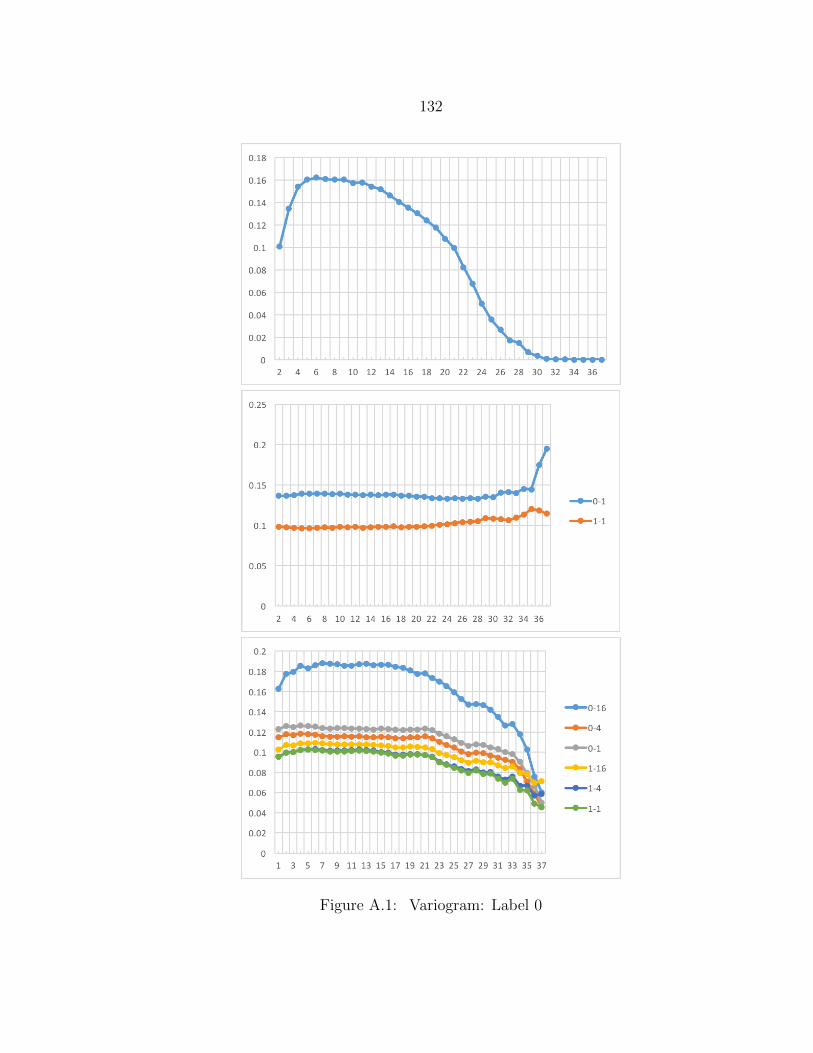
132
Figure A.1: Variogram: Label 0
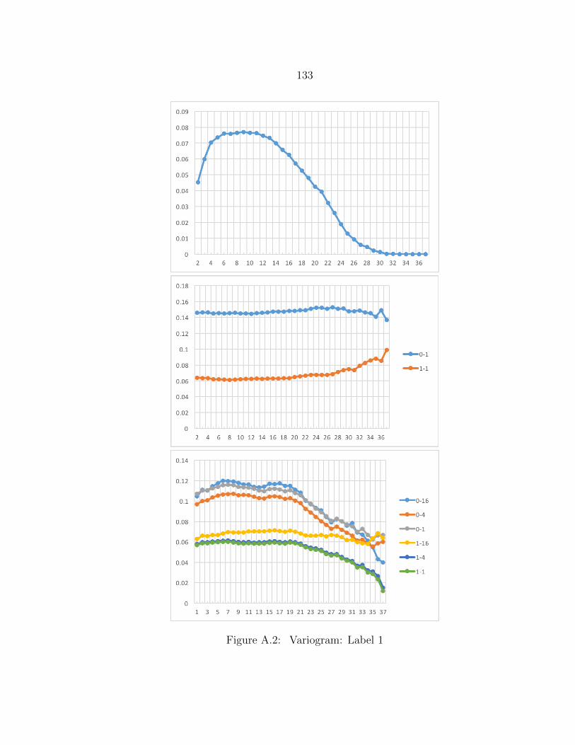
133
Figure A.2: Variogram: Label 1
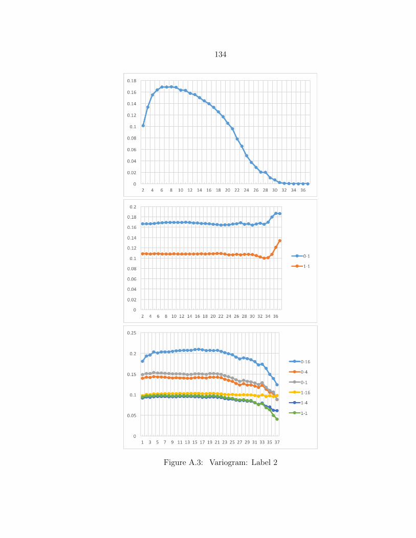
134
Figure A.3: Variogram: Label 2
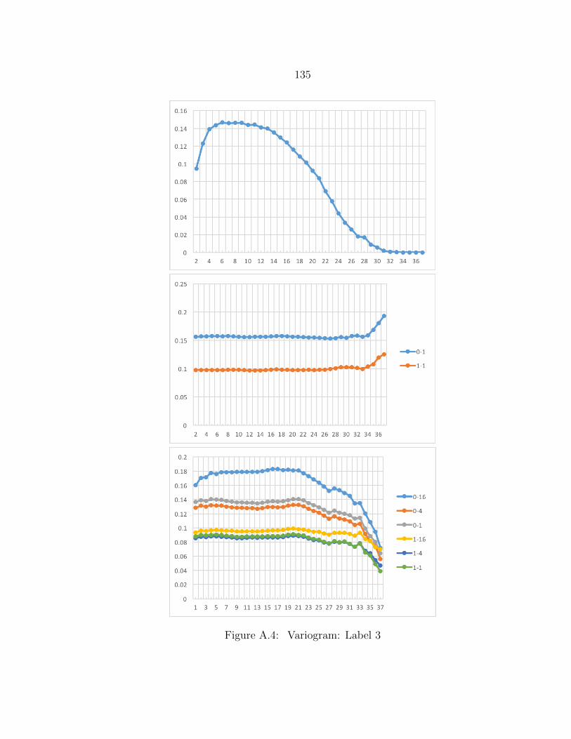
135
Figure A.4: Variogram: Label 3
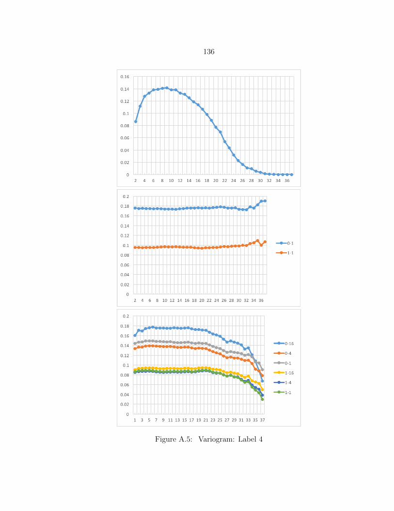
136
Figure A.5: Variogram: Label 4
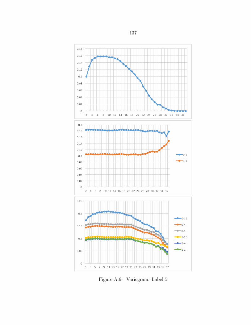
137
Figure A.6: Variogram: Label 5
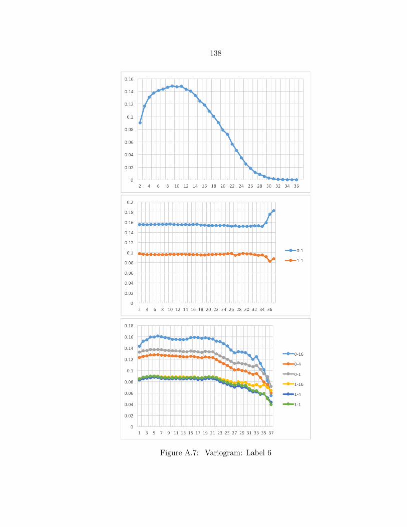
138
Figure A.7: Variogram: Label 6
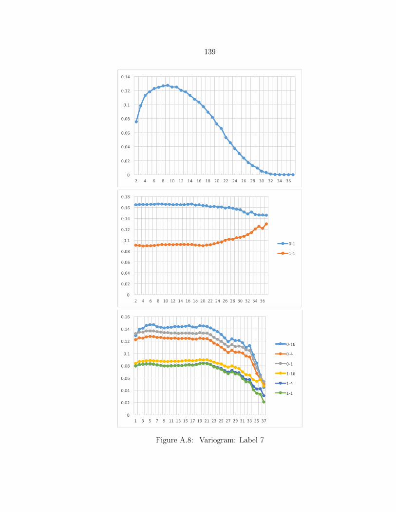
139
Figure A.8: Variogram: Label 7
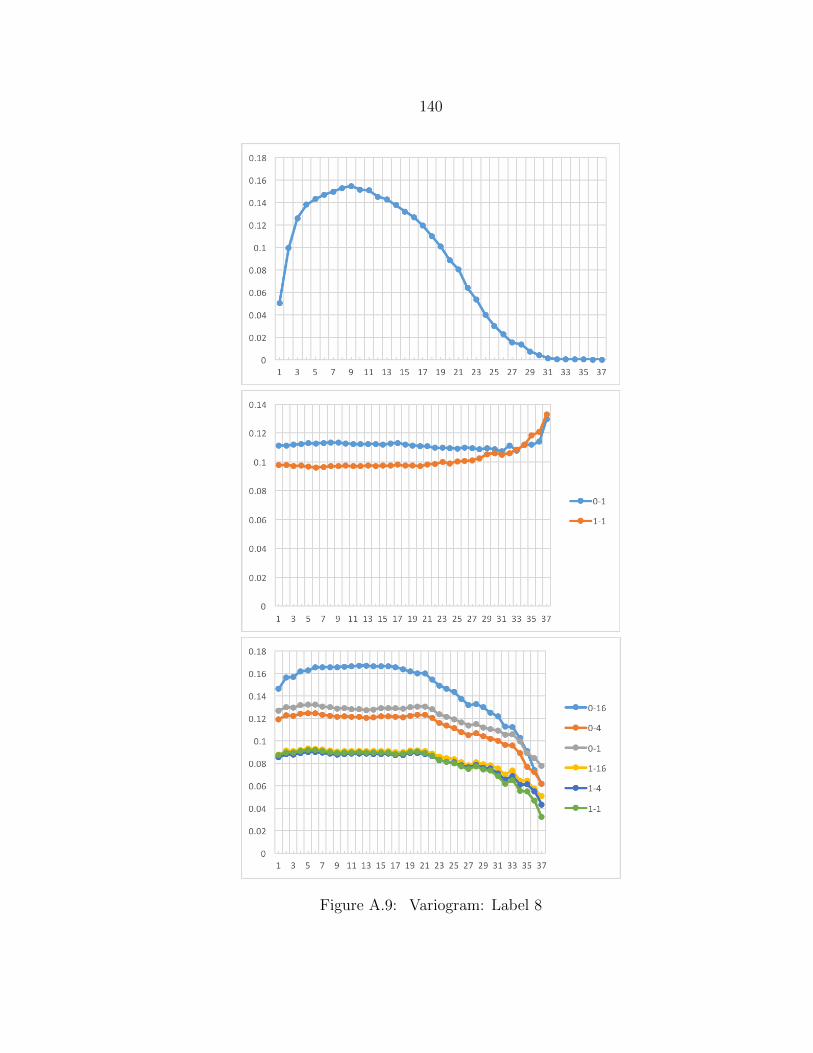
140
Figure A.9: Variogram: Label 8
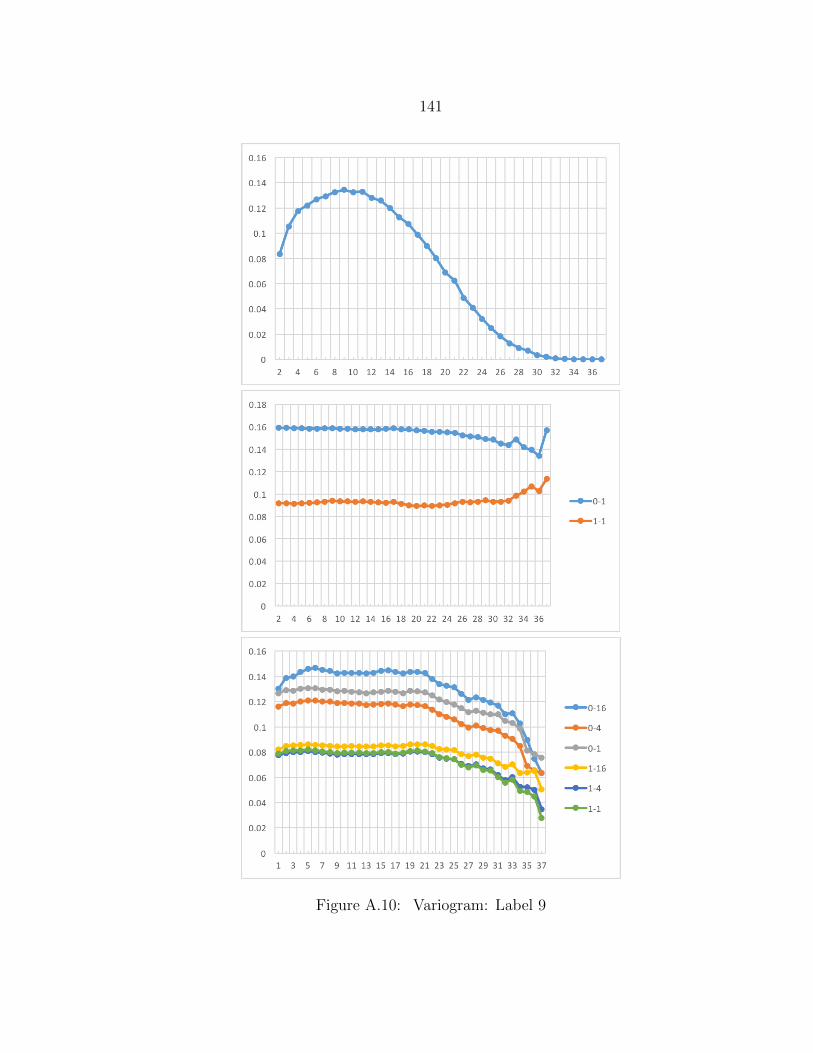
141
Figure A.10: Variogram: Label 9

142
APPENDIX B
CORRELATIONS
143
Here we include mean-correlation plots for all MNIST labels. The first row shows
correlations of the raw input vectors, the second row shows results of the Single
RBM, and the third shows results of the Partitioned-RBM. The y−axis represents
the mean correlations, and the x−axis represents Euclidean pixel distance between
points. Labels of the form N−P indicate data for hidden layer N of a Deep Belief
Network based on Partitioned-RBMs with P partitions.
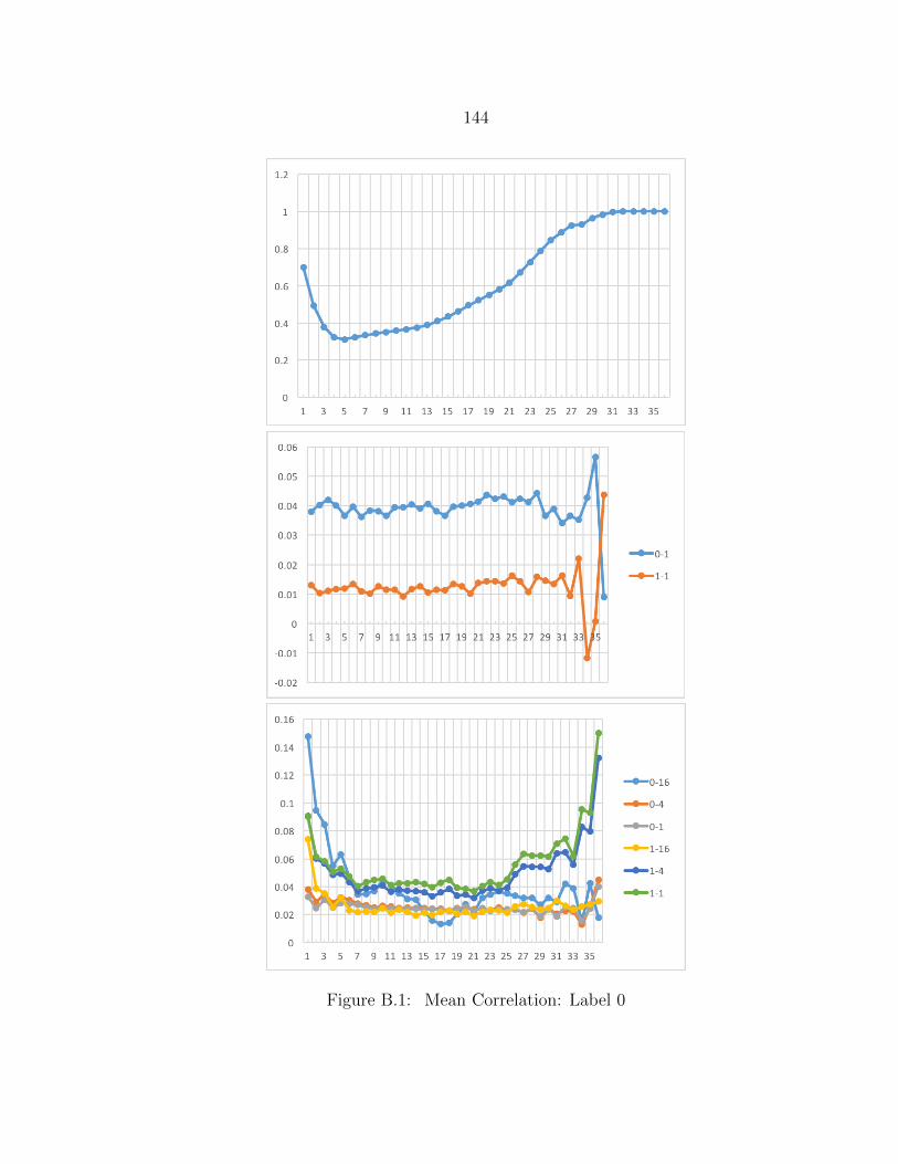
144
Figure B.1: Mean Correlation: Label 0
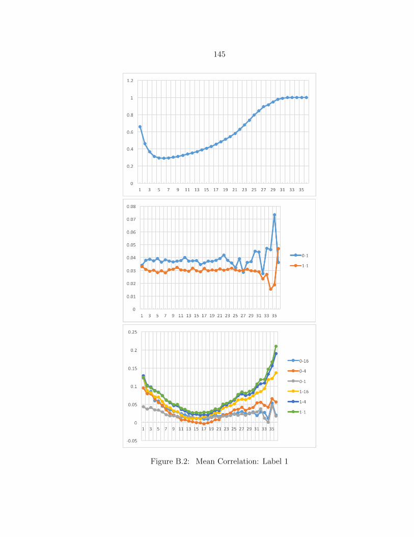
145
Figure B.2: Mean Correlation: Label 1
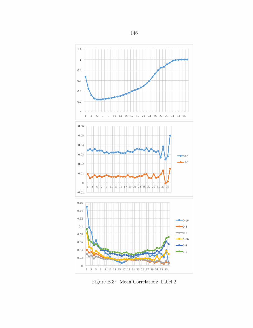
146
Figure B.3: Mean Correlation: Label 2
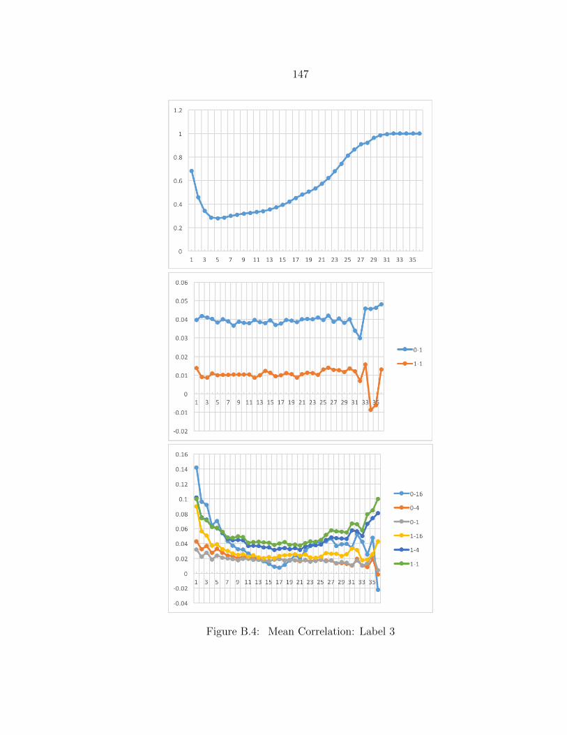
147
Figure B.4: Mean Correlation: Label 3
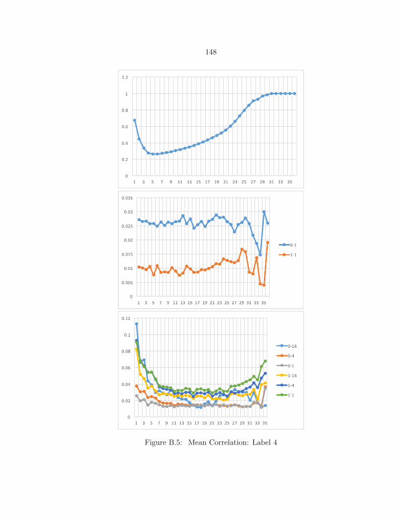
148
Figure B.5: Mean Correlation: Label 4
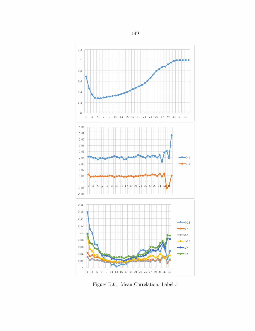
149
Figure B.6: Mean Correlation: Label 5
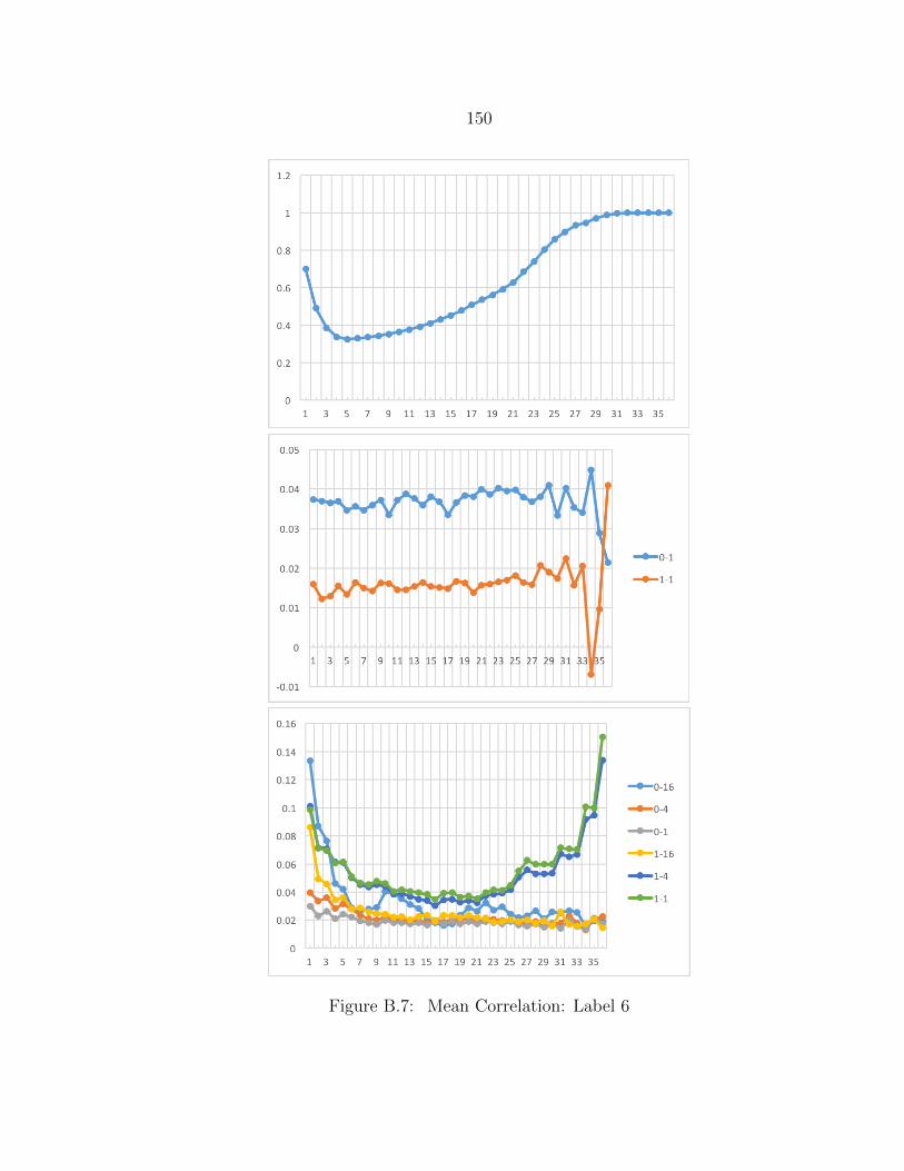
150
Figure B.7: Mean Correlation: Label 6
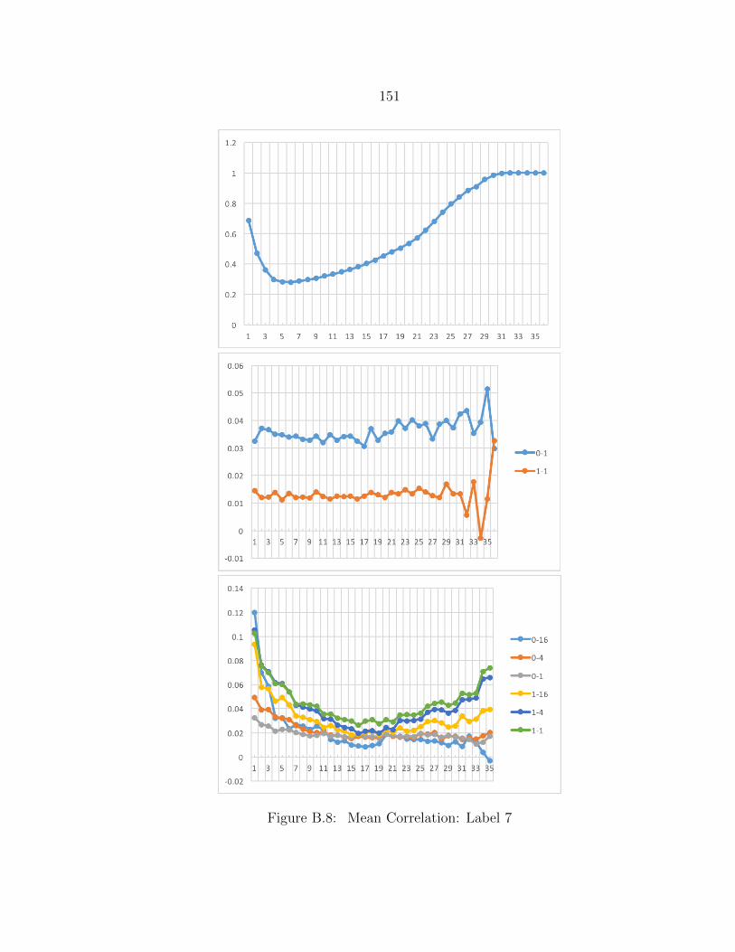
151
Figure B.8: Mean Correlation: Label 7
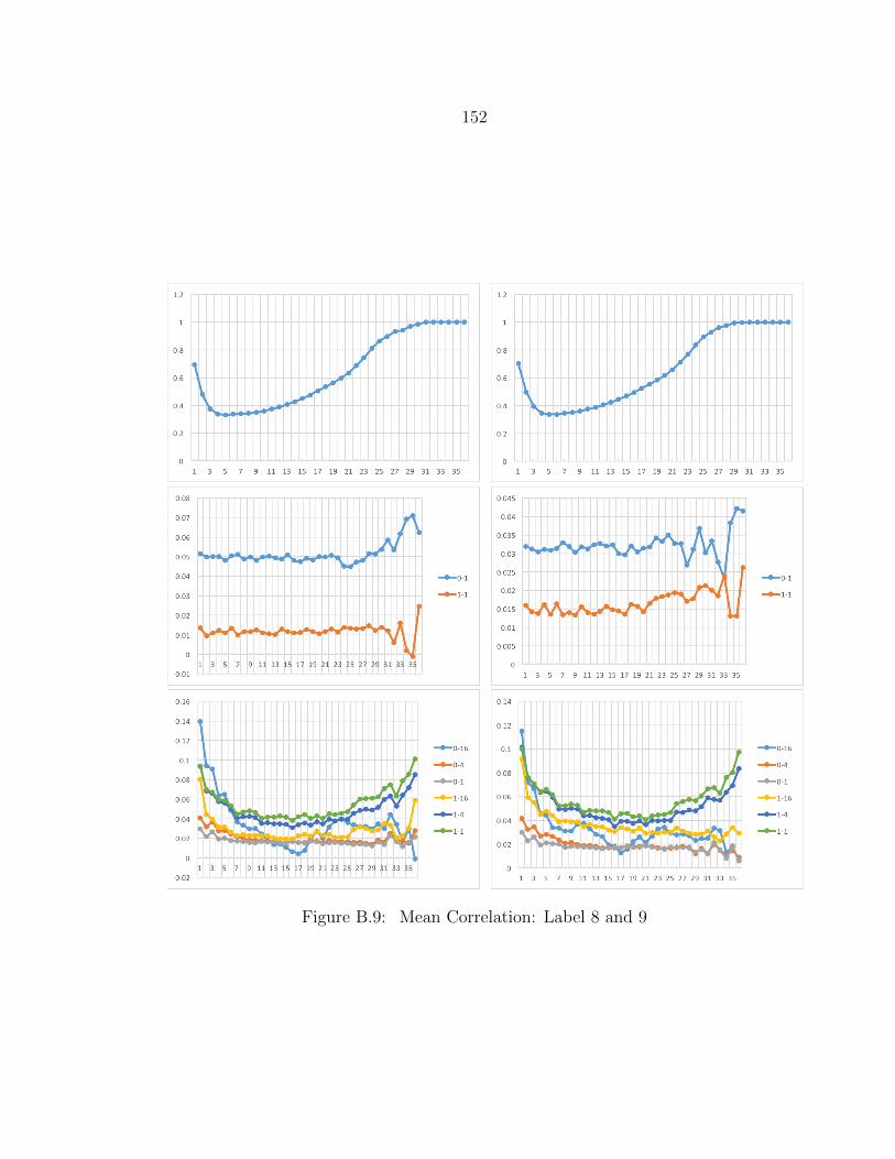
152
Figure B.9: Mean Correlation: Label 8 and 9