Embed Size (px)
Citation preview

Efficient Learning in High Dimensions with
Trees and Mixtures
Marina MeilaCarnegie Mellon University
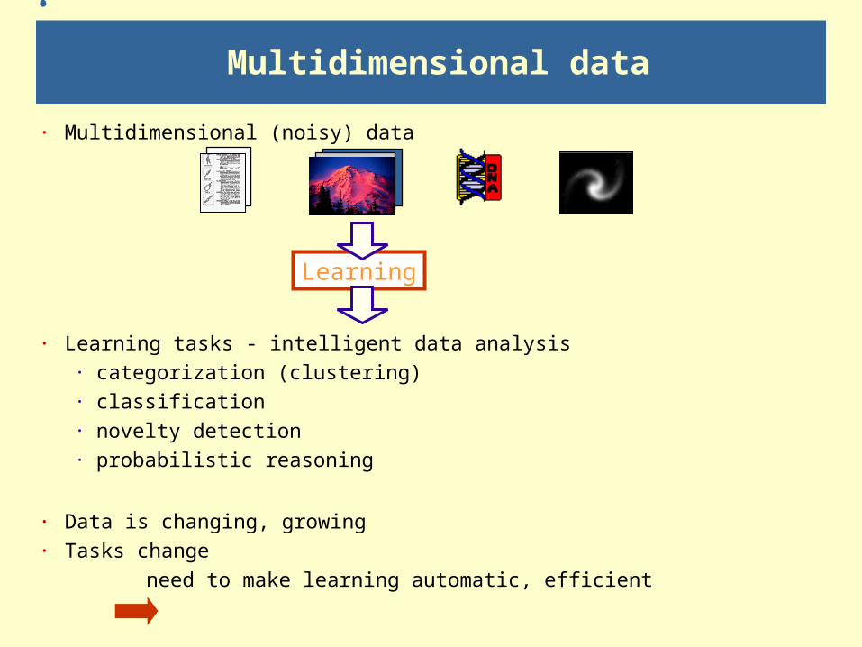
· Multidimensional (noisy) data
· Learning tasks - intelligent data analysis· categorization (clustering)· classification· novelty detection· probabilistic reasoning
· Data is changing, growing· Tasks change
need to make learning automatic, efficient
Multidimensional data
Learning
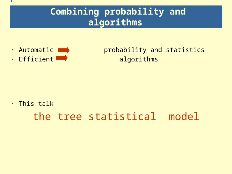
Combining probability and algorithms
· Automatic probability and statistics· Efficient algorithms
· This talk
the tree statistical model

Talk overview
Introduction:statistical models
The tree model
Mixtures of trees Learning Experiments
Accelerated learning
Bayesian learning
Perspective: generative models and decision tasks
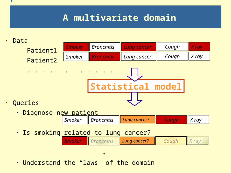
A multivariate domain
· Data
Patient1
Patient2
. . . . . . . . . . . .
· Queries
· Diagnose new patient
· Is smoking related to lung cancer?
· Understand the “laws” of the domain
Smoker X rayCoughBronchitis
Smoker X rayCoughLung cancer
Bronchitis
Smoker X rayCoughBronchitis Lung cancer?
Lung cancer?
Smoker X rayCoughLung cancer
Bronchitis
Statistical model

Probabilistic approach
· Smoker, Bronchitis .. (discrete) random variables· Statistical model (joint distribution)
P( Smoker, Bronchitis, Lung cancer, Cough, X ray )
summarizes knowledge about domain
· Queries:· inference
e.g. P( Lung cancer = true | Smoker = true, Cough = false )
· structure of the model• discovering relationships• categorization

Probability table representation
· Query:
P(v1=0 | v2=1) = = = .23
· Curse of dimensionalityif v1, v2, … vn binary variables PV1,V2…Vn table with 2n entries!
· How to represent?· How to query?· How to learn from data?· Structure?
P(v1=0, v2=1)
P(v2=1)
.14 + .03
.14 + .3 + .22 + .33
v1v2 00 01 11 00
v3
0 .01 .14 .22 .01 1 .23 .03 .33 .03

Graphical models
· Structure· vertices = variables· edges = “direct dependencies”
· Parametrization · by local probability tables
· compact parametric representation· efficient computation· learning parameters by simple formula· learning structure is NP-hard
Galaxy type
distance
photometric measuremen
t
size
observed size
spectrum Z (red-shift)dust
Obs spectrum
spectrum Z (red-shift)dust
Obs spectrum

The tree statistical model
· Structure
tree (graph with no cycles)
· Parameters
· probability tables associated to edges
1
2
3 4 5
1
2
3 4 5
T34
T3
T4|3
Tv|u(xv|xu) uv E
T(x) = Tuv(xuxv)
Tv(xv)
uv E
v V
deg v-1T(x) =
• T(x) factors over tree edges
equivalent
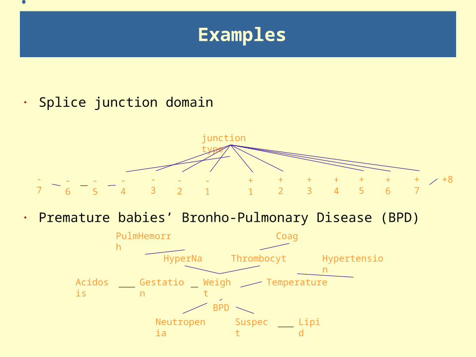
Examples
Weight
Temperature
Thrombocyt
BPDNeutropeni
aSuspect Lipid
GestationAcidosis
HyperNa
PulmHemorrh
Coag
Hypertension
-7 -5 -4 -3-6 +4
+6
+7
+5
-2 +1
+2
+3
-1
junction type
+8
· Splice junction domain
· Premature babies’ Bronho-Pulmonary Disease (BPD)

|V| =n
· computing likelihood T(x) ~ n
· conditioning TV-A|A (junction tree algorithm) ~ n
· marginalization Tuv for arbitrary u,v ~ n
· sampling ~ n· fitting to a given distribution ~ n2
• learning from data ~ n2Ndata
· is a simple model
Trees - basic operations
uv ETuv(xuxv)
Tv (xv) v V
deg v -1T(x) =
Querying the model
Estimating the model

The mixture of trees
h = “hidden” variableP( h=k ) = k k = 1, 2 . . . m
· NOT a graphical model· computational efficiency preserved
m
Q(x) = kTk(x) k=1
(Meila 97)

Learning - problem formulation
· Maximum Likelihood learning· given a data set D = { x1, . . . xN }· find the model that best predicts the data
Topt = argmax T(D)
· Fitting a tree to a distribution· given a data set D = { x1, . . . xN }
and distribution P that weights each data point, · find
Topt = argmin KL( P || T )
· KL is Kullbach-Leibler divergence· includes Maximum likelihood learning as a special case

Fitting a tree to a distribution
Topt = argmin KL( P || T )· optimization over structure + parameters
· sufficient statistics
· probability tables Puv = Nuv/N u,v V
· mutual informations Iuv
Iuv = Puv log Puv
PuPv
(Chow & Liu 68)

Fitting a tree to a distribution - solution
· StructureEopt = argmax Iuv
uv E
· found by Maximum Weight Spanning Tree algorithm with edge weights Iuv
· Parameters · copy marginals of P
Tuv = Puv for uv E
I61I23
I12
I34
I63
I45
I56

E step which xi come from T k?
distribution P k(x)
Learning mixtures by the EM algorithm
· Initialize randomly· converges to local maximum of the likelihood
M step fit T k to set of points
min KL( Pk||Tk )
Meila & Jordan ‘97

Remarks
· Learning a tree· solution is globally optimal over structures and
parameters· tractable: running time ~ n2N
· Learning a mixture by the EM algorithm· both E and M steps are exact, tractable· running time
• E step ~ mnN• M step ~ mn2N
· assumes m known· converges to local optimum
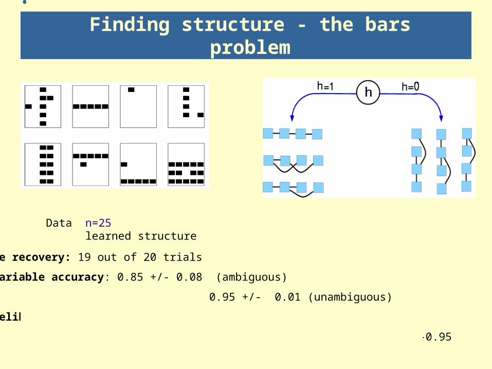
Finding structure - the bars problem
Data n=25 learned structure
Structure recovery: 19 out of 20 trials
Hidden variable accuracy: 0.85 +/- 0.08 (ambiguous)
0.95 +/- 0.01 (unambiguous)
Data likelihood [bits/data point] true model 8.58
learned model 9.82 +/-0.95
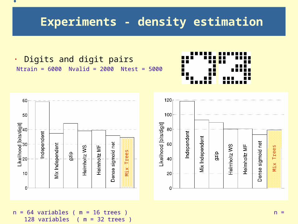
Experiments - density estimation
· Digits and digit pairs Ntrain = 6000 Nvalid = 2000 Ntest = 5000
n = 64 variables ( m = 16 trees ) n = 128 variables ( m = 32 trees )
Mix
Tre
es
Mix
Tre
es

DNA splice junction classification
· n = 61 variables· class = Intron/Exon, Exon/Intron, Neither
Tree TANB NBSupervised
(DELVE)

Discovering structure
IE junction Intron Exon
15 16 . . . 25 26 27 28 29 30 31
Tree - CT CT CT - - CT A G G
True CT CT CT CT - - CT A G G
EI junction Exon Intron
28 29 30 31 32 33 34 35 36
Tree CA A G G T AG A G -
True CA A G G T AG A G T
(Watson “The molecular biology of the gene” 87)
class
Tree adjacency matrix

Irrelevant variables
61 original variables + 60 “noise” variables
Original Augmented with irrelevant variables
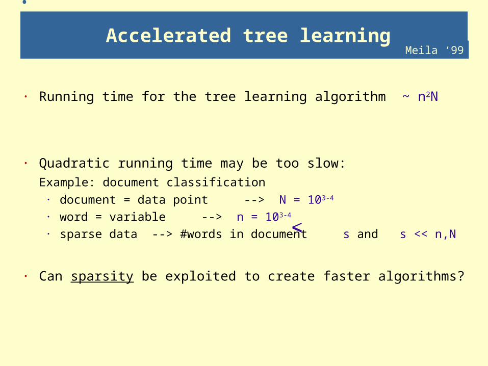
Accelerated tree learning
· Running time for the tree learning algorithm ~ n2N
· Quadratic running time may be too slow:Example: document classification· document = data point --> N = 103-4
· word = variable --> n = 103-4
· sparse data --> #words in document s and s << n,N
· Can sparsity be exploited to create faster algorithms?
Meila ‘99
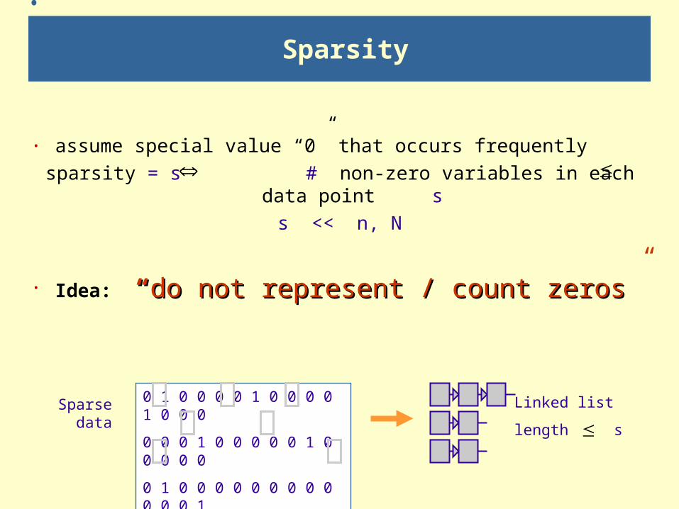
Sparsity
· assume special value “0” that occurs frequentlysparsity = s # non-zero variables in each data point s
s << n, N
· Idea: ““do not represent / count zerosdo not represent / count zeros”
0 1 0 0 0 0 1 0 0 0 0 1 0 0 0
0 0 0 1 0 0 0 0 0 1 0 0 0 0 0
0 1 0 0 0 0 0 0 0 0 0 0 0 0 1
Linked list
length s
Sparse data

Presort mutual informations
Theorem (Meila,99) If v, v’ are variables that do not cooccur with u in V (i.e. Nuv = Nuv’ = 0 ) then
Nv > Nv’ ==> Iuv > Iuv’
· Consequences
· sort Nv => all edges uv , Nuv = 0 implicitly sorted by Iuv
· these edges need not be represented explicitly· construct black box that outputs next “largest” edge

The black box data structure
list of u , Nuv > 0, sorted by Iuvlist of u , Nuv > 0, sorted by Iuv
list of u, Nuv =0, sorted by Nv list of u, Nuv =0, sorted by Nv (virtual)(virtual)
vv
vv22
vv11
vvnn
F-heap F-heap of size of size
~n~n
next edge next edge uvuv
NNvv
Total running time n log n + s2N + nK log n
(standard alg. running time n2N )

Experiments - sparse binary data
· N = 10,000· s = 5, 10, 15, 100
Standard
accelerated

Remarks
· Realistic assumption · Exact algorithm, provably efficient time bounds· Degrades slowly to the standard algorithm if data not sparse· General
· non-integer counts· multi-valued discrete variables

Meila & Jaakkola ‘00Bayesian learning of trees
· Problem· given prior distribution over trees P0(T)
data D = { x1, . . . xN }· find posterior distribution P(T|D)
· Advantages · incorporates prior knowledge · regularization
· Solution · Bayes’ formula P(T|D) = P0(T) T(xi) i=1,N
· practically hard• distribution over structure E and parameters E
hard to represent• computing Z is intractable in general• exception: conjugate priors
1Z

· want priors that factor over tree edges· prior for structure E
P0(E) uv uv E
· prior for tree parameters
P0(E) D( u|v ; N’uv ) uv E
· (hyper) Dirichlet with hyper-parameters N’uv(xuxv), u,v V· posterior is also Dirichlet with hyper-parameters
Nuv(xuxv) + N’uv(xuxv), u,v V
Decomposable priors
T = f( u, v, u|v)
uv E
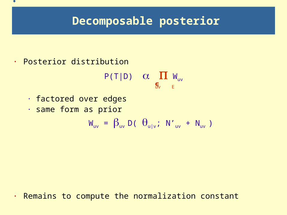
Decomposable posterior
· Posterior distribution
P(T|D) Wuv
uv E · factored over edges· same form as prior
Wuv = uv D( u|v; N’uv + Nuv )
· Remains to compute the normalization constant

The Matrix tree theorem
· Matrix tree theorem
IfP0(E) = uv, uv 0
uv E
M( ) =
1Z
v
u
v’vv'
uv
uv
Discrete: graph theorycontinuous: Meila & Jaakkola 99
Then Z = det M( )

Remarks on the decomposable prior
· Is a conjugate prior for the tree distribution· Is tractable
· defined by ~ n2 parameters· computed exactly in ~ n3 operations· posterior obtained in ~ n2N + n3 operations· derivatives w.r.t parameters, averaging, . . . ~ n3
· Mixtures of trees with decomposable priors· MAP estimation with EM algorithm tractable
· Other applications· ensembles of trees· maximum entropy distributions on trees
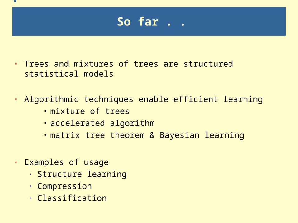
So far . .
· Trees and mixtures of trees are structured statistical models
· Algorithmic techniques enable efficient learning • mixture of trees• accelerated algorithm• matrix tree theorem & Bayesian learning
· Examples of usage· Structure learning· Compression· Classification
Generative models and discrimination
· Trees are generative models · descriptive· can perform many tasks suboptimally
· Maximum Entropy discrimination (Jaakkola,Meila,Jebara,’99)
· optimize for specific tasks· use generative models· combine simple models into ensembles· complexity control - by information theoretic principle
· Discrimination tasks· detecting novelty · diagnosis· classification

Bridging the gap
Descriptive learning
Discriminative learning
Tasks

Future . . .
· Tasks have structure· multi-way classification· multiple indexing of documents· gene expression data· hierarchical, sequential decisions
Learn structured decision tasks· sharing information btw tasks (transfer)· modeling dependencies btw decisions