Efficient Global Gravity Determination from

Satellite-to-Satellite Tracking (SST)

by

Shin-Chan Han

Report No. 467

Geodetic and GeoInformation ScienceDepartment of Civil and Environmental Engineering and Geodetic Science

The Ohio State UniversityColumbus, Ohio 43210-1275

September 2003

Efficient Global Gravity Determination from

Satellite-to-Satellite Tracking (SST)

By

Shin-Chan Han

Report No. 467Geodetic and Geoinformation Science

Department of Civil and Environmental Engineering and Geodetic ScienceThe Ohio State University

Columbus, Ohio 43210-1275

September 2003

ii

ABSTRACT

By the middle of this decade, measurements from the CHAMP (CHAllenging of Minisatellite Payload)and GRACE (Gravity Recovery And Climate Experiment) gravity mapping satellite missions areexpected to provide a significant improvement in our knowledge of the Earth's mean gravity field and itstemporal variation. For this research, new observation equations and efficient inversion method weredeveloped and implemented for determination of the Earth’s global gravity field using satellitemeasurements. On the basis of the energy conservation principle, in situ (on-orbit) and along trackdisturbing potential and potential difference observations were computed using data fromaccelerometer- and GPS receiver-equipped satellites, such as CHAMP and GRACE. The efficientiterative inversion method provided the exact estimates as well as an approximate, but very accurateerror variance-covariance matrix of the least squares system for both satellite missions.

The global disturbing potential observable computed using 16-days of CHAMP data was used todetermine a 50×50 test gravity field solution (OSU02A) by employing a computationally efficientinversion technique based on conjugate gradient. An evaluation of the model using independentGPS/leveling heights and Arctic gravity data, and comparisons with existing gravity models, EGM96and GRIM5C1, and new models, EIGEN1S and TEG4 which include CHAMP data, indicate thatOSU02A is commensurate in geoid accuracy and, like other new models, it yields some improvement(10% better fit) in the polar region at wavelengths longer than 800 km.

The annual variation of Earth’s gravitational field was estimated from 1.5 years of CHAMP data andcompared with other solutions from satellite laser ranging (SLR) analysis. Except the second zonal andthird tesseral harmonics, others second and third degree coefficients were comparable to SLR solutionsin terms of both phase and magnitude. The annual geoid change of 1 mm would be expected mostlydue to atmosphere, continental surface water, and ocean mass redistribution. The correlation betweenCHAMP and SLR solutions was 0.6~0.8 with 0.7 mm of RMS difference. Although the result shouldbe investigated by analyzing more data for longer time span, it indicates the significant contribution ofCHAMP SST data to the time-variable gravity study.

Considering the energy relationship between the kinetic and frictional energy of the satellite and thegravitational potential energy, the disturbing potential difference observations can be computed from theorbital state vector, using high-low GPS tracking data, low-low satellite-to-satellite GRACEmeasurements, and data from 3-axis accelerometers. Based on the monthly GRACE simulation, thegeoid was obtained with an accuracy of a few cm and with a resolution (half wavelength) of 160 km.However, the geoid accuracy can become worse by a factor of 6~7 because of spatial aliasing. Theapproximate error covariance was found to be a very good accuracy measure of the estimatedcoefficients, geoid, and gravity anomaly. The temporal gravity field, representing the monthly meancontinental water mass redistribution, was recovered in the presence of measurement noise and high

iii

frequency temporal variation. The resulting recovered temporal gravity fields have about 0.2 mm errorsin terms of geoid height with a resolution of 670 km.

It was quantified that how significant the effects due to the inherent modeling errors and temporalaliasing caused by ocean tides, atmosphere, and ground surface water mass are on monthly meanGRACE gravity estimates. The results are based on simulations of GRACE range-rate perturbationsdue to modeling error along the orbit; and, their effects and temporal aliasing on the estimatedgravitational coefficients were analyzed by fully inverting monthly simulated GRACE data. For oceantides, the study based on the model difference, CSR4.0–NAO99, indicates that some residualconstituents like in S2 may cause errors 3 times larger than the measurements noise at harmonic degreesless than 15 in the monthly mean estimates. On the other hand, residual constituents in K1, O1, and M2

are reduced by monthly averaging below the measurement noise level. For the atmosphere, thedifference in models, ECMWF–NCEP, produces errors in GRACE range-rate measurements as strongas the measurement noise. They corrupt all recovered coefficients and introduce 30 % more error in theglobal monthly geoid estimates up to maximum degree 120. However, the analysis based on dailyCDAS-1 data for continental surface water mass redistribution indicates that the daily soil moisture andsnow depth variations affect the monthly mean GRACE recovery less than the measurement noise.

iv

PREFACE

This report was prepared by Shin-Chan Han, a graduate student, Department Civil and EnvironmentalEngineering and Geodetic Science, under the supervision of Professors C. Jekeli and C.K. Shum.

This research is supported by grants from the Center for Space Research, University of Texas under aprime contract from NASA (CSR/GRACE #735367), and from NASA's Solid Earth and NaturalHazards Program (NASA/GRACE #736312).

This report was also submitted to the Graduate School of Ohio State University as a thesis in partialfulfillment of the requirements for the degree Doctor of Philosophy.

v

ACKNOWLEDGMENTS

Most of all, I wish to express my deepest gratitude to Drs. C. Jekeli and C.K. Shum for support,encouragement, patience and intellectual insight throughout this research. Their broad knowledge andkeen intuition have wisely guided my work. I would like to express my sincere thanks to Dr. D.Grejner-Brzezinska for thoughtful reviews and comments of this dissertation. Some interestingdiscussion for the application with Dr. R. R. B. von Frese (Geological Sci., OSU, Ohio) is appreciated.Dr. W. Bosch (DGFI, Munich, Germany) stimulated me to pursue finding the error covariance from theiterative solution method. Unique lectures from Dr. H. Sünkel (TUG, Graz, Austria) and Dr. B.Schaffrin provided me valuable mathematical and statistical foundation of this research. Our geodesygroup (people in laboratory for space geodesy and remote sensing) is very supportive, and I thank all ofthem for assisting me and for just being themselves.

This research is supported by grants from the Center for Space Research, University of Texasunder a prime contract from NASA, and from NASA's Solid Earth and Natural Hazards Program. Ialso acknowledge computational resources awarded by the Ohio Supercomputing Center.

vi

TABLE OF CONTENTSPAGE

ABSTRACT..................................................................................................................................... ii

PREFACE....................................................................................................................................... iv

ACKNOWLEDGMENTS................................................................................................................ v

LIST OF TABLES..........................................................................................................................xiii

LIST OF FIGURES ........................................................................................................................ ix

CHAPTERS:

1. INTRODUCTION .................................................................................................................. 11.1 Summary and Expected Contributions ................................................................................ 31.2 Organization ...................................................................................................................... 3

2. ENERGY INTEGRAL AND CONJUGATE GRADIENT FOR EFFICIENT RECOVERY OFTHE EARTH GRAVITY FIELD FROM SATELLITES .......................................................... 62.1 Energy integrals in the inertial and rotating frames ................................................................ 62.2 Efficient inversion method for a large linear system ............................................................ 112.2.1 Linear model for geopotential ........................................................................................ 112.2.2 Block diagonally dominant normal matrix ....................................................................... 122.2.3 Conjugate gradient with a preconditioner ....................................................................... 12

3. GLOBAL GRAVITY FIELD RECOVERY USING IN SITU POTENTIAL OBSERVABLEFROM CHAMP ................................................................................................................... 193.1 Introduction ..................................................................................................................... 193.2 Observation equation ....................................................................................................... 203.2.1 Scale, bias, and bias drift in accelerometer data ............................................................. 213.2.2 Empirical forces in orbit data ......................................................................................... 223.3 Results and analysis .......................................................................................................... 233.3.1 Geopotential model using 16 days of CHAMP RSO and accelerometer data ................. 233.3.2 Geopotential models using dynamic, reduce-dynamic, and kinematic CHAMP orbits andaccelerometer data ................................................................................................................. 303.3.3 On the use of a pre-conditioning matrix as an error variance-covariance matrix .............. 363.3.4 Temporal variation of monthly CHAMP solutions .......................................................... 443.4 Conclusion ....................................................................................................................... 543.4.1 OSU02A ...................................................................................................................... 54

vii

3.4.2 Gravity solutions from dynamic, reduced-dynamic, and kinematic orbits ......................... 553.4.3 Approximate error covariance ....................................................................................... 553.4.4 Temporal (annual) variation of the Earth gravity field ...................................................... 56

4. THE EFFICIENT DETERMINATION OF GLOBAL GRAVITY FIELD FROM SATELLITE-TO-SATELLITE TRACKING MISSION, GRACE ............................................................. 574.1 Introduction ..................................................................................................................... 574.2 In situ observable ............................................................................................................. 584.2.1 Satellite-to-satellite tracking measurements .................................................................... 584.2.2 In situ potential observable ............................................................................................ 594.2.3 In situ potential difference observable ............................................................................ 594.3 Observation model and characteristics of the normal matrix ............................................... 614.3.1 Linear observation model for potential difference ........................................................... 614.3.2 Block-diagonally dominant normal matrix ....................................................................... 634.4 Efficient solution method for a large linear system .............................................................. 664.4.1 Direct least-squares solution and its computational cost .................................................. 664.4.2 Conjugate gradient with a preconditioner ....................................................................... 674.4.3 Speed-up by truncated Taylor series ............................................................................. 684.5 Results ............................................................................................................................. 714.5.1 Static gravity field recovery ........................................................................................... 714.5.2 Approximate accuracy and covariance .......................................................................... 744.5.3 Time-variable gravity field recovery ............................................................................... 784.6 Conclusion ....................................................................................................................... 81

5. TIME-VARIABLE EFFECTS OF OCEAN TIDES, ATMOSPHERE, AND CONTINENTALWATER MASS ON MONTHLY MEAN GRACE GRAVITY FIELD ................................. 825.1 Introduction ..................................................................................................................... 825.2 Data and method ............................................................................................................. 835.2.1 Models for ocean tides .................................................................................................. 835.2.2 Models for atmosphere ................................................................................................. 845.2.3 Models for continental surface water ............................................................................. 855.3 Ocean tides ..................................................................................................................... 865.4 Atmosphere ..................................................................................................................... 925.5 Continental surface water ................................................................................................. 985.6 Summary and conclusion ................................................................................................ 1025.6.1 Ocean tide .................................................................................................................. 1025.6.2 Atmosphere ................................................................................................................ 1025.6.3 Continental surface water ............................................................................................ 103

6. CONCLUSION ................................................................................................................. 105

REFERENCES ........................................................................................................................... 107

viii

LIST OF TABLESPAGE

3.1 Gravity model assessment using GPS-leveling data (Standard deviations in cm) ....................... 29

3.2 Gravity model assessment using Arctic gravity anomalies data [Kenyon and Forsberg, 2001] (unit:mgal) ..................................................................................................................................... 29

3.3 Accelerometer calibration and empirical force parameters (daily estimates) .............................. 31

3.4 Gravity model assessments using Arctic gravity anomalies data provided by NIMA .............. 36

3.5 The correlation coefficients between the two geoid variation maps of two temporal gravitysolutions ................................................................................................................................ 54

3.6 The root mean square (RMS) of the geoid variations of three solution sets ............................... 54

3.7 The RMS of difference between two geoid variation maps of two temporal gravity solutions .... 54

5.1 Summary of time-variable gravity effects on the monthly mean GRACE gravity field ............... 104

ix

LIST OF FIGURESPAGE

2.1 Two convergence factors: (2.44) and (2.53) ........................................................................... 17

3.1 (i) Difference between kinetic energy and a priori model, EGM96 (solid), (ii) Friction energycomputed from STAR accelerometer data (dashed) ................................................................ 24

3.2 Difference between kinetic energy and the a priori model, EGM96 (dotted); and friction energycomputed from STAR accelerometer data (solid) (mean and trend are removed) ..................... 25

3.3 Degree variance of EGM96 signal (solid black) and difference between intermediate iterations andEGM96 ................................................................................................................................. 26

3.4 Degree variance of differences between two gravity models: GRIM5C1-OSU02A (solid blue),EGM96-OSU02A (dashed red), TEG4-OSU02A (dotted blue), EIGEN1S-OSU02A (dot-solidblack) .................................................................................................................................... 27

3.5 Geoid difference (RMS over all longitude) between two gravity models: GRIM5C1-OSU02A(dotted black), EGM96-OSU02A(solid blue), TEG4-OSU02A(dashed red), EIGEN1S-OSU02A(dot-solid black) ..................................................................................................... 28

3.6 Spectrum of potential difference between EGM96 and orbit data with and without the empiricalforce model ........................................................................................................................... 30

3.7 In situ potential difference with respect to EGM96 in terms of a height anomaly ....................... 32

3.8 Degree variance of differences between four reference gravity models and the gravity solution fromthe CSR dynamic orbit ........................................................................................................... 33

3.9 Degree variance of differences between four reference gravity models and the gravity solution fromthe GFZ dynamic orbit ........................................................................................................... 34

3.10 Degree variance of differences between EGM96 gravity model and gravity solutions from JPLreduced dynamic and ESA kinematic orbits ............................................................................ 35

3.11 Global geoid difference (RMS over all longitude bands) between two gravity models ............... 35

3.12 Square root of degree variance of Kaula rule, EGM96, monthly CHAMP solution, and true andapproximate standard deviations of the CHAMP solution ........................................................ 37

x

3.13 Relative error (in percents) of approximate standard deviation of the CHAMP solution ............ 38

3.14 The predicted geoid error from; (Top) true error covariance matrix, (Middle) approximate errorcovariance matrix, (Bottom) approximate error variance ......................................................... 39

3.15 The predicted gravity anomaly error from; (Top) true error covariance matrix, (Middle)approximate error covariance matrix, (Bottom) approximate error variance ............................ 40

3.16 The differences (true and approximate error covariance) of the predicted geoid error (Top) andthe gravity anomaly error (Bottom) ......................................................................................... 41

3.17 The predicted radial orbit error versus the inclination from; (i) true error covariance matrix, (ii)approximate error covariance matrix, (iii) EGM96 covariance matrix ....................................... 42

3.18 Predicted radial orbit error versus the spherical harmonic order from; (i) true error covariancematrix, (ii) approximate error covariance matrix, (iii) EGM96 covariance matrix

.............................................................................................................................................. 43

3.19 The standard deviation of EGM96 per degree and for a monthly CHAMP solution, and the geoiddifference between two consecutive monthly CHAMP solutions .............................................. 44

3.20 The CHAMP ground track pattern for a month in-between April and May, 2001 (Top) and 2002(Bottom) ................................................................................................................................ 44

3.21 The monthly mean variations of ocean, ground surface water, and atmosphere over a month; thestandard deviation of a monthly mean CHAMP solution; the annual gravity field variationdetermined from SLR (4x4 solution) ....................................................................................... 45

3.22 The times series of temporal (annual) variations of the Earth’s gravitational coefficients, C20, C21,and S21 from SLR and CHAMP ........................................................................................... 47

3.23 The times series of temporal (annual) variations of the Earth’s gravitational coefficients, C22, S22,and C30 from SLR and CHAMP ........................................................................................... 48

3.24 The times series of temporal (annual) variations of the Earth’s gravitational coefficients, C31, S31,and C32 from SLR and CHAMP ........................................................................................... 49

3.25 The times series of temporal (annual) variations of the Earth’s gravitational coefficients, S32, C33,and S33 from SLR and CHAMP ........................................................................................... 50

xi

3.26 The cosine component of the temporal (annual) variations of the Earth’s gravitation in terms of thegeoid; (Top) SLR, Nerem et al., 2000; (Middle) SLR, Cheng et al., 2002; (Bottom) CHAMPsolutions. ............................................................................................................................... 52

3.27 The sine component of the temporal (annual) variations of the Earth’s gravitation in terms of thegeoid; (Top) SLR, Nerem et al., 2000; (Middle) SLR, Cheng et al., 2002; (Bottom) CHAMPsolutions. ............................................................................................................................... 53

4.1 Example of ascending arc of a GRACE satellite’s orbit (inclination = 89 degrees), referencelongitude, and longitude correction. ......................................................................................... 64

4.2 Structure of the block diagonal normal matrix. ......................................................................... 65

4.3 Structure of the normal matrix for realistic GRACE orbit (Nmax=30, logarithmic scale). ...........66

4.4 Pairs of observation points within one pair of co-latitude bands after re-ordering (part of onemonth data with a sampling rate of 0.1 Hz). ............................................................................ 69

4.5 Error in potential difference computation due to using Taylor series in the computation ofassociated Legendre functions. ............................................................................................... 71

4.6 Square root of averaged degree variances of EGM96, its error, errors of the first and last (15th)iterates. .................................................................................................................................. 73

4.7 Monthly mean geoid error from GRACE (RMS over all longitudes) with and without the spatialaliasing. .................................................................................................................................. 74

4.8 (Top) The estimated coefficient error, approximate standard deviation, true standard deviation;(Bottom) The relative error of approximate standard deviation (Nmax=90 and 10 days of data). 75

4.9 The error of estimated geoid based on the true EGM96 geoid; and the σ and 3σ confidencebounds of the predicted geoid accuracy based on an approximate covariance (Nmax=90, 10 daysof data, and no spatial aliaing). ................................................................................................ 76

4.10 The estimated coefficient error and approximate standard deviation with and without the spatialaliasing (Nmax=120 and 30 days of data). .............................................................................. 77

4.11 The error of estimated geoid based on the true EGM96 geoid; and the σ and 3σ confidencebounds of the predicted geoid accuracy based on an approximate covariance (Nmax=120, 30days of data, and no spatial aliasing). ...................................................................................... 77

xii

4.12 (Left): Monthly mean continental surface water mass redistribution on Jan., 2001. (Right): Thecorresponding geoid change ................................................................................................... 79

4.13 Square root of averaged degree variances of MWSA, DWSA, and monthly GRACE(approximate) error. ............................................................................................................... 80

4.14 (Left) Recovered monthly mean continental surface water mass redistribution in terms of the geoidheight (Nmax=30); (Right) Its difference from the true geoid due to MWSA. ........................... 80

5.1 Degree variances of four mean ocean tidal constituent errors, monthly mean temporal gravitysignals, and monthly GRACE sensitivity in terms of the geoid. .................................................. 87

5.2 Height anomaly errors at a single satellite induced by the mean tidal model errors. (a) K1(Top-left), (b) O1(Top-right), (c) M2(Bottom-left), and (d) S2(Bottom-right). ............................... 88

5.3 The mean tidal model error existing in GRACE measurements in terms of the range-rate; (a) K1,(b) O1, (c) M2, and (d) S2. ................................................................................................... 88

5.4 The time-varying tidal model errors computed along GRACE orbit for 30 days in terms of therange-rate; (a) K1, (b) O1, (c) M2, and (d) S2. ..................................................................... 89

5.5 The time-varying tidal model errors (after Gaussian smoothing) computed along GRACE orbit for30 days in terms of the range-rate; (a) K1, (b) O1, (c) M2, and (d) S2. .................................. 90

5.6 Degree variances of errors existing in the recovered spherical harmonic coefficients. ............... 92

5.7 Order variances of errors existing in the recovered spherical harmonic coefficients. ............... 92

5.8 Degree variances of atmospheric mass redistributions; daily ECMWF, ECMWF–NCEP, dailyECMWF–NCEP, and GRACE monthly sensitivity. ................................................................ 93

5.9 Global effects on the geoid of (a) daily ECMWF, (b) ECMWF–NCEP (snapshot), (c) dailyECMWF–NCEP, (d) Time-varying atmospheric modeling error in terms of GRACE range-ratefor a month (mapped with respect to the leading satellite). ....................................................... 94

5.10 Degree variances (a) and order variances (b) of recovered coefficients in the case of noise onlyand noise combined with residual atmospheric perturbation. .................................................... 96

5.11 Errors in the geoid height (Nmax=30) due to noise only (a) and noise with residual atmosphericperturbation (b). ..................................................................................................................... 97

xiii

5.12 Degree variances (m = 30, 31, 32, and 33) of errors in the geoid height (a); Order variances (30 ≤n ≤ 90) of errors in the geoid height (b). .................................................................................. 98

5.13 The monthly mean water storage anomaly on January, 2001. ................................................... 99

5.14 The perturbation in the GRACE range-rate measurements due to daily variability of WSA for amonth .................................................................................................................................... 99

5.15 The degree variances of monthly mean WSA, its daily variability with respect to MWSA, and theexpected monthly GRACE error in terms of the geoid height. ................................................ 100

5.16 The degree variances of the ‘truth’ MWSA, its recoveries, and the aliasing effect. ............ 101

5.17 The ‘truth’ geoid change (a); The recovered geoid change (b); The effect of noise and aliasing (c);The aliasing effect only (d). ................................................................................................... 102

1

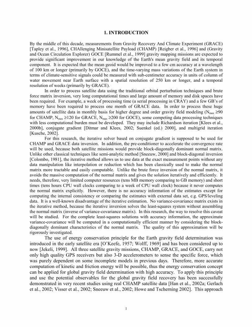
1. INTRODUCTION By the middle of this decade, measurements from Gravity Recovery And Climate Experiment (GRACE) [Tapley et al., 1996], CHAllenging Minisatellite Payload (CHAMP) [Reigber et al., 1996] and (Gravity and Ocean Circulation Explorer) GOCE [Rummel et al., 1999] gravity mapping missions are expected to provide significant improvement in our knowledge of the Earth's mean gravity field and its temporal component. It is expected that the mean geoid would be improved to a few cm accuracy at a wavelength of 100 km or longer (primarily by GOCE), and the time-varying mass variations of the Earth system in terms of climate-sensitive signals could be measured with sub-centimeter accuracy in units of column of water movement near Earth surface with a spatial resolution of 250 km or longer, and a temporal resolution of weeks (primarily by GRACE).

In order to process satellite data using the traditional orbital perturbation techniques and brute force matrix inversion, very long computational times and large amount of memory and disk spaces have been required. For example, a week of processing time (a serial processing in CRAY) and a few GB’s of memory have been required to process one month of GRACE data. In order to process these huge amounts of satellite data in monthly basis for higher degree and order gravity field modeling (Nmax ≥90 for CHAMP, Nmax ≥120 for GRACE, Nmax ≥200 for GOCE), some competing data processing techniques with less computational burden must be developed. They may include Richardson iteration [Klees et al., 2000b], conjugate gradient [Ditmar and Klees, 2002; Suenkel (ed.) 2000], and multigrid iteration [Kusche, 2002].

For this research, the iterative solver based on conjugate gradient is supposed to be used for CHAMP and GRACE data inversion. In addition, the pre-conditioner to accelerate the convergence rate will be used, because both satellite missions would provide block-diagonally dominant normal matrix. Unlike other classical techniques like semi-analytic method [Sneeuw, 2000] and block-diagonal inversion [Colombo, 1981], the iterative method allows us to use data at the exact measurement points without any data manipulation like interpolation or reduction which has been classically used to make the normal matrix more tractable and easily computable. Unlike the brute force inversion of the normal matrix, it avoids the massive computation of the normal matrix and gives the solution iteratively and efficiently. It needs, therefore, very limited computer resources (tens MB memory comparing to GB memory) and short times (tens hours CPU wall clocks comparing to a week of CPU wall clock) because it never computes the normal matrix explicitly. However, there is no accuracy information of the estimates except for computing the internal consistency or comparing the estimates with external data set, e.g. GPS/leveling data. It is a well-known disadvantage of the iterative estimation. No variance-covariance matrix exists in the iterative method, because the iterative inversion solves the least-squares system without assembling the normal matrix (inverse of variance-covariance matrix). In this research, the way to resolve this caveat will be studied. For the complete least-squares solutions with accuracy information, the approximate variance-covariance will be computed in a computationally efficient manner by considering the block-diagonally dominant characteristics of the normal matrix. The quality of this approximation will be rigorously investigated.

The use of energy conservation principle for the Earth gravity field determination was introduced in the early satellite era [O’Keefe, 1957; Wolff, 1969] and has been considered up to now [Jekeli, 1999]. All three satellite gravity missions, CHAMP, GRACE, and GOCE, carry not only high quality GPS receivers but also 3-D accelerometers to sense the specific force, which was purely dependent on some incomplete models in previous days. Therefore, more accurate computation of kinetic and friction energy will be possible, thus the energy conservation concept can be applied for global gravity field determination with high accuracy. To apply this principle and use the potential observables for the global gravity field recovery has been successfully demonstrated in very recent studies using real CHAMP satellite data [Han et al., 2002a; Gerlach et al., 2002; Visser et al., 2002; Sneeuw et al., 2002; Howe and Tscherning 2002]. This approach

2

has many advantages, because it is more direct method requiring no integration of equation of motion, all observables are used as in situ measurements (boundary values in boundary value problem), and it allows alternate correction models, e.g., tides or atmosphere, to be efficiently used to assess their accuracies (e.g., modeling errors or aliasing effects), and to validate monthly data product, specifically for GRACE mission. In this research, this concept will be applied with an efficient inversion to determine the global gravity field from CHAMP and GRACE data.

Currently, studies on Earth gravity field are being revolutionized with the aid of new satellite missions, CHAMP and GRACE, carrying very high precision instruments. The CHAMP gravity and magnetic mapping satellite mission, launched in July 2000 by the GeoForschungsZentrum (GFZ), Potsdam, Germany, provides the first data set with high-low satellite tracking and accelerometer measurements for gravity field studies. CHAMP’s orbit is at an altitude of 450 km and its 87° inclination enables near-global coverage. Its payload includes geodetic-quality, Blackjack-class, GPS receivers (16-channel, dual-frequency) with multiple antennas for precise orbit determination and atmospheric limb-sounding, and the 3-axis STAR accelerometer (3x10-9 m/s2 and 3x10-8 m/s2 precision in the along track or cross track, and radial directions, respectively [Perret et al., 2001]) to measure non-conservative forces including atmospheric drag. The GRACE launched on March 17, 2002 for a mission span of 5 years or longer. The mission consists of two identical co-orbiting spacecrafts with a separation of 220±50 km at a mean initial orbital altitude of 500 km with a circular orbit and an inclination of 890 for near-global coverage [Thomas, 1999; GRACE Science Mission Requirement Document, 2000; Bettadpur and Watkins, 2000]. The scientific objectives of GRACE include the mapping and understanding of climate-change signals associated with mass-variations within solid Earth – atmosphere – ocean – cryosphere - hydrosphere system with unprecedented accuracy and resolution in the form of time-varying gravity field [e.g., Wahr et al., 1998]. New models of Earth’s static as well as time-variable gravity field will be available every 30 days for 5 years. In this research, it is expected to obtain new Earth gravity models and their possible temporal variations based on actual CHAMP data using the energy conservation principle together with the iterative inversion technique. CHAMP gravity solutions will be assessed with other independent data including GPS/leveling and Arctic gravity anomaly data. The contribution and weakness of CHAMP solutions to temporal gravity field models will be studied. In addition, the time-variable gravity fields (ocean, hydrology, tide, and atmosphere) will be studied based on GRACE simulation and full inversion. The previous simulation studies, e.g., Wahr et al.(1998), Nerem et al.(2002), and Wahr and Velicogna (2002), use the spherical harmonic coefficients for ocean and ground water hydrology and add random noise to the coefficients according to the GRACE error degree variance model [Bettadpur and Watkins, 2000], assuming independently and identically distributed errors among the coefficients of the same degree. Then, they take spatial averaging in a spectral domain to reduce higher degree and order errors and obtain the long wavelength signal of temporal gravity. These currently published simulations fall short of a full inversion of GRACE data, as properly mentioned by Wahr and Velicogna, (2002). It is limited to the analysis in the spectral domain and hardly describes the temporal aliasing problem that exists in the monthly mean gravity field.

Here, a more direct and appropriate approach to obtain temporal gravity fields is suggested based on the energy conservation principle and iterative inversion. By adding the temporal gravity signals to the GRACE measurements for a month, the spherical harmonic coefficients will be estimated complete up to degree and order of 120 in the presence of both measurement noises and temporal gravity signals by fully inverting monthly GRACE data. In

3

the previous studies, it is not yet known how the temporal variations of ocean, hydrology, and atmosphere affect monthly mean GRACE gravity products. This study will quantify the ocean tidal, hydrological, and atmospheric modeling error and their temporal aliasing effects in the measurement domain; and it will discuss how they corrupt the monthly mean GRACE gravity field in both spatial and spectral domains. 1.1 Summary and Expected Contributions The primary objective is to develop a fast solver for geopotential determination with accuracy information. In a “brute force” way (the way in which no data manipulation like gridding is required), extremely demanding computer resources are required to estimate the spherical harmonic coefficients. The developed method should reduce computational costs and process monthly satellite data efficiently. Compared to other approaches such as [Tapley et al., 2002; Reigber et al., 2002], it will produce monthly mean gravity field considerably faster with very limited memory and storage requirements. While the previous studies including [Kless et al., 2000b; Ditmar and Klees, 2002; Suenkel (ed.) 2000; Kusche, 2002] do not provide an accuracy of the estimates, the developed method will produce not only the exact solutions but also reasonably accurate variance-covariance approximates without extra computational cost. The secondary objective is to use the in situ potential observable at satellite altitude to estimate the global gravity field. This simple but powerful concept was already introduced in early days [Wolff, 1969; Wagner, 1983], but was not able to be tested at that time. Unlike the traditional gravity field determination methodologies [Tapley et al., 2002; Reigber et al., 2002], the use of the in situ potential observable through the energy conservation principle has several advantages: 1) no numerical integration; 2) no initial state problem; 3) separate processing of the orbit and gravity parameter estimation; 4) linear relationship between the unknown geopotential coefficients and the observations. It, however, relies on the precise orbits determined prior to the gravity recovery. With these advantages, the energy conservation approach will be applied to determine the global gravity field very efficiently.

The third objective is to study static and temporal gravity fields by analyzing long period CHAMP data and simulated GRACE data based on the energy conservation principle and the developed fast solver. The feasibility of time-variable gravity recovery associated with the ocean, atmosphere, and hydrology will be studied by fully inverting the observations, unlike the limited approaches in the spectral domain, e.g. Wahr et al.(1998) and Nerem et al.(2002), which do not involve any inversion.

The fourth objective is to analyze the time-variable effects of atmosphere, ocean tides, and continental surface water on the monthly mean GRACE gravity field. The temporal resolution of the GRACE products is limited to a month, because of the accuracy requirement and data coverage. It is expected that the temporal aliasing due to time-variable gravity corrupts the monthly mean GRACE products significantly. No previous study about this aliasing effect on the monthly field is available, because the current studies on time-variable gravity are limited to spectral domain analyses, e.g. Wahr et al.(1998); Nerem et al.(2002); and Wahr and Velicogna (2002); and Velicogna et al. (2002). In this research, the temporal aliasing effects will be rigorously studied in the spatial and spectral domains. 1.2 Organization

4

Three (more or less) independent chapters (Chapters 3, 4, and 5) contain full descriptions of each theme from introduction to conclusion. Besides the current introductory Chapter, this dissertation is organized as follows: Chapter 2. Energy integral approach and conjugate gradient method from the efficient recovery of the Earth gravity field from satellites

This chapter presents detailed derivations for the gravitational potential computations starting from Newton’s second law of the motion. Two different versions of formulas are developed for the potential computation using the position, velocity vectors, and the specific (action) force vector in the inertial and any arbitrary rotating frames. In addition, this Chapter shows comprehensive derivations of the conjugate gradient method with a pre-conditioner for the least squares system. It discusses the error norm to be minimized and the optimal search direction to the least-squares solution. The developed method will be used for an inversion method of the previously derived observation equations for the gravitational potential.

Chapter 3. Global gravity field recovery using in situ potential observable from CHAMP

This Chapter describes CHAMP data processing results for the recovery of Earth’s geopotential coefficients. It discusses the accelerometer data calibration, empirical force parameters, and static gravity recovery from dynamic, reduced dynamic, and kinematic orbits. The quality assessment of the determined gravity fields is presented based on independent data such as GPS/leveling and Arctic gravity anomaly. The approximate error covariance matrix is computed very efficiently in terms of both computational time and storage. The quality of this approximation is investigated for the terrestrial and orbital applications. Finally, this Chapter shows the temporal gravity field estimated from the times series of monthly mean CHAMP solutions. The estimated annual component is compared with the currently available solution from SLR.

Chapter 4. Efficient determination of global gravity field from satellite-to-satellite tracking mission, GRACE

Chapter 4 discusses the extension of the energy integral incorporating the range-rate measurements expected from the GRACE mission. It describes an efficient solution strategy for the fast recovery of high degree geopotential models. In addition to the static gravity field recovery, it discusses the high degree spatial aliasing, the use of approximate error covariance, and the time-variable gravity field recovery.

Chapter 5. Time-variable effects of ocean tides, atmosphere, and continental water mass on monthly mean GRACE gravity field

Chapter 5 contains an extensive study of the temporal aliasing of the monthly mean GRACE gravity estimates. How the high frequency temporal variability of residual ocean tides, residual atmosphere, and hydrology signals affect the monthly mean gravity field is investigated.

Chapter 6. Conclusion

5

Main contributions of this dissertation are summarized in Chapter 6 and further remaining investigations are also suggested.

6

2. ENERGY INTEGRAL AND CONJUGATE GRADIENT FOR EFFICIENT RECOVERY OF THE EARTH GRAVITY FIELD FROM SATELLITES

2.1. Energy integrals in the inertial and rotating frames Newton’s second law of motion under the influence of Earth’s gravitational field in the inertial frame is expressed as:

iii fgx +=&& , (2.1) where the superscript, i, indicates that the quantity refers to the inertial frame. x&& is the acceleration (second time-derivative of position) vector, g is the gravitation vector, and f is the specific force vector (force per unit mass). While Jekeli (1999) derived the energy integral based on Lagrange’s equation for the motion considering the Hamiltonian, hereafter the energy integral will be derived directly by integrating (2.1). In addition, the energy integral will be derived in the rotating frame, attached to the rotating Earth. First, consider the inner product between the velocity vector, ix& , and the acceleration vector, ix&& , coordinatized in the inertial frame as follows:

iiiiiii )t),t(( fxxgxxx ⋅+⋅=⋅ &&&&& , (2.2) The gravitational acceleration is a function of the position, )t(ix , (which depends on the time) and possibly time, t. The left-hand side can be expressed as follows:

=

⋅=⋅

2iiiii

21

21 xxxxx &&&&&&

dtd

dtd . (2.3)

The gravitational vector is the gradient of the gravitational potential, V, with respect to the position vector:

i

iiii t)),t(V(t)),t(V()t),t(( i

xxxxg x ∂

∂=∇= . (2.4)

The first term of the right-hand side of (2.2) can be denoted using (2.4) as:

i

iiiiiii t)),t(V(t)),t(V()t),t(( i

xxxxxxgx x ∂

∂⋅=∇⋅=⋅ &&& . (2.5)

Consider the total derivative of t)),t(V( ix with respect to t, then we will have the following:

7

tt)),t(V(

t)t(t)),t(V(

tt)),t(V( ii

i

ii

∂∂+

∂∂= xx

xxx

dd

dd . (2.6)

Noting that t

)t(ii

ddxx =& , (2.5) can be represented as follows:

tt)),t(V(

tt)),t(V()t),t((

iiiii

∂∂−=⋅ xxxgx

dd

& . (2.7)

Combining (2.3) and (2.7) into (2.2), we have

iiii2i

tt)),t(V(

tt)),t(V(

21 fxxxx ⋅+

∂∂−=

&&d

ddtd . (2.8)

By integrating (2.8) with respect to t, we obtain

Cttt

t)),t(V(t)),t(V(21 t

t

iit

t

ii2i

00

+⋅+∂

∂−= ∫∫ dd fxxxx && , (2.9)

where C is the integral constant (energy constant of the system). Therefore, the gravitational potential in the inertial frame can be computed as follows:

Ctt

t)),t(V(t21t)),t(V(

t

t

it

t

ii2ii

00

−∂

∂+⋅−= ∫∫ dd xfxxx && . (2.10)

The first term of the right-hand side is the kinetic energy, in which the velocity is needed for the computation. The second term is the friction energy due to the action force. The third term is the energy caused by the time variation of the gravitational field in the inertial frame. This is the same equation appearing in the equation (1) of Jekeli (1999) derived from a different approach. If there are no specific forces (e.g., the body is freely falling in a vacuum in the gravitational field), no Earth rotation, and no explicit temporal variation in the gravitational field, the second and third terms disappear and (2.10) reduces to:

const.C))t(V(21 i2i ==− xx& . (2.11)

This implies the sum of the kinetic and (negative) potential energy is conserved, which is the energy conservation principle. Note that the negative sign in the potential term stems from the definition of the potential and field. In physical geodesy, a field is defined as the gradient of the potential [Heiskanen and Moritz, 1966], while physicists define a field as the negative gradient of a potential [Arfken and Weber, 1995].

8

Jekeli (1999) rigorously investigated the third term in the right-hand side of (2.10), and concluded that this term is dominantly caused by the Earth’s rotation. He called it the potential rotation accounting for the rotation of the potential in the inertial frame. With a reasonable approximation, it is

)(ωtt

t)),t(V( i1

i2

i2

i1e

t

t

i

0

xxxxd && −−≈∂

∂∫

x , (2.12)

where ωe is the Earth’s rotation rate, ),,( i

3i2

i1

i xxx=x , and ),,( i3

i2

i1

i xxx &&&& =x . It should be emphasized that the only approximation occurring in the implementation of (2.10) with (2.12) for the Earth gravity field stems from ignoring the explicit temporal gravitational variations due to tides, loading effects, and other geodynamical phenomena and frictional forces like atmospheric drag, solar radiation pressure, and so on. However, their effects are seven or eight order of magnitude smaller than the Earth rotation for the computation of the left-hand side of (2.12) [Jekeli, 1999]. The integral equation (2.10), called the energy integral, can be re-formulated in any arbitrary frame. Here, we express the gravitational potential in a rotating frame such as the Earth fixed frame. The position vector in the rotating frame (designated by the superscript, r), rx , is obtained by multiplying the corresponding rotation matrix, r

iC , as follow:

iri

r C xx = , (2.13) where r

iC is a rotation matrix from the inertial frame to the rotating frame, in the same context, irC is the rotation matrix from the rotating frame to the inertial frame. Considering the

relationships rir

i C xx = , rir

i C gg = , and rir

i C ff = , the equation (2.1) is expressed in the rotating frame as:

rrrir2

2ri )C(

tC fgx +=

dd . (2.14)

Note that i

rC and riC depend on the time explicitly. This fact introduces the Coriolis (force)

effect and centrifugal force in the expression of Newton’s equation of motion. In order to develop the left-hand side of (2.14), consider the following:

rir

rir

rir CC)C(

txxx && +=

dd , (2.15a)

rir

rir

rir

rir

rir

rir2

2CC2C)CC(

t)C(

txxxxxx &&&&&&&& ++=+=

dd

dd . (2.15b)

The time-derivative of the rotation matrix can be computed by considering the differential equation of the transformation (Jekeli, 2001). That is,

9

[ ]×= r

irir

ir CC ω& , (2.16)

where r

irω is the angular velocity of the rotating frame with respect to the inertial frame coordinatized in the rotating frame. × is the operator for the cross product, and [ ]×r

irω represents a skew-symmetric matrix with appropriate elements of r

irω . Taking one more time differentiating and assuming r

irω is constant, we get:

[ ][ ]××= rir

rir

ir

ir CC ωω&& . (2.17)

Putting (2.16) and (2.17) to (2.15b),

rir

rrir

ir

rrir

rir

ir

rir2

2CC2C )C(

txxωxωωx &&& +×+××=

dd . (2.18)

Putting (2.18) to (2.14), Newton’s second law of motion in the rotating frame (with a constant rotating rate) is expressed as the follows:

rrir

rrir

rir

rrr 2 xωxωωfgx &&& ×−××−+= . (2.19) Comparing this with (2.1), we have two additional terms, the centrifugal and Coriolis accelerations. Consider the potential of the centrifugal and gravitational forces. That is,

r

rrir t)),t(V(t)),t(V()t),t(( r

xxxxg x ∂

∂=∇= , (2.20)

( ) ( )2rrirr

2rrir

rrir

rir 2

121

r xωx

xωxωω x ×∂∂−=×−∇=×× . (2.21)

Multiplying rx& to (2.19) and combining it with (2.20) and (2.21), the following is obtained:

( ) )(221t)),t(V( rr

irr2rr

irrrrr

r

rrrr xωxxω

xxfx

xxxxx &&&&&&&& ×⋅−×

∂∂⋅+⋅+

∂∂⋅=⋅ . (2.22)

The last term of the right-hand side drops out, because of the inner product of two perpendicular vectors is zero. Considering the equation (2.6), we have

tt)),t(V(

tt)),t(V(t)),t(V( rr

r

rr

∂∂−=

∂∂⋅ xx

xxx

dd

& , (2.23)

( ) ( ) ( )2rrir

2rrir

2rrirr

r

ttxωxωxω

xx ×

∂∂−×=×

∂∂⋅

dd

& . (2.24)

10

Combining (2.23) and (2.24) to (2.22), we have the following:

( ) ( ) rr2rrir

2rrir

rr2r

t21

t21

tt)),t(V(

tt)),t(V(

21

tfxxωxωxxx ⋅+×

∂∂−×+

∂∂−=

&&dd

dd

dd . (2.25)

The fourth term drops out because there is no explicit dependence on time. By integrating (2.25) with respect to t, we obtain,

( ) ∫ ∫ +⋅+∂

∂−×+=t

t

t

t

rrr2rr

irr2r

0 0

Cttt

t)),t(V(21t)),t(V(

21 dd fxxxωxx && . (2.26)

With the same approximation as in (2.12), the third term in the right-hand side of (2.26) is dropped because t)),t(V( rx doesn’t have the effect due to Earth rotation. Instead, the Earth rotation effect appears in the second term of the right-hand side in (2.26). Finally, we obtained the energy integral equation in the rotating frame as follows:

( ) C21t

21t)),t(V(

2rrir

t

t

rr2rr

0

−×−⋅−= ∫ xωfxxx d&& . (2.27)

In the same level of approximation as in (2.10), we may write ( )Te

rir ω00=ω . Then, (2.27)

becomes

( ) ( ) Cxxω21t

21t)),t(V(

2r2

2r1

2e

t

t

rr2rr

0

−

+−⋅−= ∫ dfxxx && . (2.28)

Both friction energy terms, the second terms on the right-hand sides of (2.10) and (2.28), can be computed in two ways considering the following relationships:

∫∫ ⋅=⋅t

t

iit

t

ii

00

t xfxf dd& , (2.29a)

∫∫ ⋅=⋅t

t

rrt

t

rr

00

t xfxf dd& . (2.29b)

The first approach is to integrate the inner product between the specific force vector, f, and the velocity vector, x& , over time. The second approach is to integrate the specific force vector along the orbit over the trajectory. These energy integral equations can be used to compute the in situ gravitational potentials along the trajectory of any satellite or even airplane carrying GPS, accelerometer, and attitude sensors.

11

2.2. Efficient inversion method for a large linear system 2.2.1 Linear model for geopotential The (derived) observations of the potential using either (2.10) or (2.28) with the position, velocity, and specific forces being measured, can be used to estimate the Earth geopotential field. The relationship between the in situ potential measurements and the harmonic geopotential coefficients (after truncation) is:

+

+=

+

= =∑ ∑ V

nm

Vnm

nm

1nNmax

2n

n

0m Smλsin

Cmλcos)θ(cosP

rR

RGM

rGM)λθ,,r(V , (2.30)

where GM is the gravitational constant times the Earth’s mass, R is the Earth’s mean radius, (r,θ,λ) are the coordinates of the satellite, nmP is the fully normalized, associated Legendre function of degree n and order m, and V

nmC and VnmS are the unknown spherical harmonic

coefficients of degree n and order m. The coefficients for the first degree harmonic, V1,0C , V

1,1C ,

and V1,1S , vanish by setting the origin of the coordinate system at the center of mass [Heiskanen

and Moritz, 1967]. It is very common to introduce the reference (known) field like GRS80 [Moritz, 1992] in order to make the (total) potential observations the residual (or disturbing) potentials. GRS80 is constructed using 4 defining constants; 1) the equatorial radius of the Earth, 2) the geocentric gravitational constant of the Earth, GMGRS80, 3) the Earth’s flattening, 4) the angular velocity of the Earth. Based on these parameters, the normal potential, U, is computed as follows:

∑∞

=

+

+=

n)even for (only 2n

GRS80n0n0

1nGRS80GRS80Cmλcos)θ(cosP

rR

RGM

rGM)λθ,,r(U , (2.31)

where GRS80

nmC (only for even n) are computed using the above defined quantities. In most cases, only five (n=2,4,6,8, and 10) coefficients are enough to compute U very accurately. Most of the Earth gravitational potential is contributed from this normal potential. The Earth’s gravitational constant, GM, is can be modeled as unknown, however, in this study, it is fixed as GMGRS80. Therefore, the disturbing potential of Earth’s gravitation is defined as in (2.32) and given as in (2.33):

)λθ,,r(U)λθ,,r(V)λθ,,r(T −= , (2.32)

+

=

+

= =∑ ∑

nm

nmnm

1nNmax

2n

n

0m SmλsinCcosmλ

)θ(cosPrR

RGM)λθ,,r(T , (2.33)

12

where, GM=GMGRS80, nmC and nmS are the same coefficients as VnmC and V

nmS , except even degree zonal coefficients, n0C (n is even), in which case, nmC is equal to V

nmC minus GRS80nmC .

The coefficients, nmC and nmS , are unknown parameters to be estimated in a (linear) least-squares sense by solving the corresponding normal equations based on (2.33). Let y be the vector of observations, T, which can be computed using the energy integral and the normal potential (GRS80). The parameter vector, x, contains the (disturbing) geopotential coefficients up to a certain maximum degree and order, Nmax. Then, we will have the exact linear relationship between the disturbing potential observations and the unknown coefficients such as xAy ⋅= . The parameter vector is ordered as follows:

TmaxN10 ][ xxxx L= , (2.34) where T

mNmax,m1,mmm,mNmax,m1,mmm,m ]SSSCCC[ LL ++=x and the superscript,

T, denotes the transpose of the column vector. The design matrix, A, is computed based on the exact observation equations given in (2.33). If we order the unknown parameters as in (2.34), the normal matrix may be dominantly block diagonal. That is, the proper ordering of the unknowns may enhance the condition of the normal matrix. 2.2.2 Block diagonally dominant normal matrix Colombo (1983) describes that the normal matrix becomes a block diagonal matrix, if the unknown coefficients are ordered as in (2.34), and the observations are gridded on a sphere with longitude-independent errors. Therefore, it is very easy and fast to compute and invert the normal matrix. While the satellite measurements definitely do not provide gridded observations at the same altitude, they may approximately satisfy the conditions by Colombo (1983). The radius of the satellite can be approximately constant (actually, the satellite altitude varies within a few tens of km). Consider the observations in a certain latitude band. The longitude interval of the observations in the latitude band is approximately the same, because the Earth rotation rate is quite constant. The potential ‘measurement’ errors are expected to be homogeneous and (possibly) uncorrelated over the globe. These facts and the orthogonality of the harmonic sine and cosine functions induce large cancellations in the off-diagonal blocks of the normal matrix, which correspond to different spherical harmonic orders. Therefore, the resulting normal matrix based on the satellite measurements tends to be dominantly block diagonal. 2.2.3 Conjugate gradient with a preconditioner For a low-degree gravity model such as Nmax=50, the direct solution is possible through the Cholesky decomposition or the brute-force inversion of the normal matrix after it is accumulated on the basis of all measurements of T. However, in this study, the conjugate gradient method is applied to determine the least-squares estimates iteratively, with the block-diagonal part of the normal matrix serving as a pre-conditioner. The accumulation and inversion of the block-diagonal part of the normal matrix are considerably faster than those of the full normal matrix. The conjugate gradient method is one of most popular iterative methods to solve the large linear system of equations efficiently. This method always converges if the normal matrix is

13

positive definite or full rank [Golub and van Loan, 1996]. The essential idea of this method is as follows. The initial iterate (vector) is updated by adding the increment (vector) to the previous iterate. The direction of the increment vector (or updating vector) is determined as the optimal direction toward the minimum error, which is the gradient direction of squared error norm with an appropriate weight matrix. Finding and adding new increment vectors based on previously determined increment vectors and previous iterates, the intermediate solution vector gradually approaches and finally converges to the true solution vector. This method produces practically the same solution as the direct least-squares method, but by not going through the matrix inversion. The rate of convergence (which is a critical concern for efficiency issue) depends on the condition number of the normal matrix and can be improved by conditioning the linear system of equations in the preliminary step. The proper choice of a preconditioning matrix, i.e., preconditioner, should be done by considering the efficiency between computing the preconditioner and reducing the condition number of the linear equation system or normal matrix. Here, the conjugate gradient algorithm is derived for least-squares problems and its convergence rate is discussed. In the least-squares procedure, we frequently meet the normal equation system given as follows:

cξN =ˆ , (2.35) where N is the normal matrix, ξ is the estimate of the unknown parameters, and c is the vector involving the observation vector. By setting up and inverting the positive-definite normal matrix, N, we can obtain ξ , which is a direct approach. The estimate and its covariance matrix are given by

120

1 σ}ˆD{ ,ˆ −− == NξcNξ . (2.36) The weight matrix, inverse of the cofactor matrix, of the estimate is simply N. This straightforward approach requires enough memory and computation time. That may limit the size of linear system with a full matrix. If we are interested in having the estimates only, then the estimates (vector) can be computed iteratively without setting up and inverting the normal matrix, which thus would be very efficient. Assume we have any guess of the estimate (or just zero guess), iξ . The error (or difference) vector between the solution, ξ , and the guess (or the intermediate iterate, in general),

iξ , is given as follow:

cNξξξe 1iii

ˆ −−=−= . (2.37) The squared norm of the error vector with respect to the weight matrix of the estimate, which is just the matrix, N, is a function of iξ and given by

( ) ( )cNξNcNξξ 1i

T1ii 2

1)φ( −− −−= . (2.38)

14

Now we want to update or correct iξ to obtain the next iterate, 1i+ξ , that is closer to ξ . First, we need to find the direction along which ϕ decreases fastest. Second, the location is found as long as the minimum of ϕ is guaranteed along that direction. The direction is determined by the negative gradient of )φ( iξ , i.e., )φ( iξ∇− . Not surprisingly, this is exactly the same direction as the residual vector, ri.

iii

iφ)φ( rNξcξ

ξ =−=∂∂−=∇− . (2.39)

Now, iξ is updated along the direction of ri. That is, iii1i rξξ λ+=+ . To find the location, a parameter, iλ , should be determined to provide minimum )φ( 1i+ξ .

( ) ( ) iTiii

Ti

2ii

1iii

T1iii1i 2

1)φ(21)φ( rrNrrξcNrξNcNrξξ λλλλ −+=−+−+= −−

+ . (2.40)

The condition, )φ()φ( i1i ξξ ≤+ , indicates 021

iTiii

Ti

2i ≤− rrNrr λλ . Let )f( iλ be )φ()φ( i1i ξξ −+ .

To find iλ where )f( iλ has minimum, take derivative of )f( iλ with respect to iλ .

0fi

Tii

Tii

i=−=

∂∂ rrNrrλλ

, (2.41)

iTi

iTi

i Nrrrr

=∴λ . (2.42)

Therefore, the updated solution vector is found by

iii1i rξξ λ+=+ , (2.43) where ii Nξcr −= and i

Tii

Tii Nrrrr=∴λ .

The convergence rate of this method (using the residual vectors in order to update the intermediate iterates) after some arithmetic can be shown to be as follows:

)φ(κ11)φ( 1-ii ξξ

−≤ , (2.44)

where κ is the condition number of the normal matrix, N, and ξξξξ0 is the initial vector. However, it could produce very slow convergence if the condition number is large. Actually, the direction of residual vector assures finding the locally (not globally) optimal direction towards minimum error norm, because the residual vectors can be proved to be orthogonal to each other disregarding the shape or structure of the error norm (See the following lemma).

15

Lemma 1. The residual vectors are perpendicular to each other. That is, ij

2ij

Ti δrrr = where ijδ

is 0 if i≠j and is 1 if i=j. Proof)

2ii

Ti

iTi

iTi

iTi

iTii

Tiii

Ti1i

Ti

iiiiii1i1i

0α

αα

rrr

NrrNrrrrrrNrrrrrr

NrrNrNξcNξcr

=

=−=−=

−=−−=−=

+

++

To obtain the algorithm to produce a better convergence rate, we should consider to use N-orthogonal vectors, which are denoted by pi’s, instead of using the residual vectors, ri’s. They assure the globally optimal direction towards minimum error norm because they are N-orthogonal. We compute the vector, pi, with the previously determined vectors, ri-1 and pi-1, based on the condition of the N-orthogonality. That is, ijj

Ti δc ⋅=Npp , where ijδ is 0 if i≠j and

is 1 if i=j, and c is a non-zero scalar value. First, express pi as a sum of previously determined vectors like:

1-ii1-ii β prp += , (2.45) Second, N-orthogonality is applied to (2.45) in order to obtain the coefficients, βi:

( ) 0β 1-ii1-iT

1iiT

1i =+= −− prNpNpp ,

1-iT

1i

1-iT

1iiβ Npp

Nrp

−

−−=∴ . (2.46)

However, the expression of βi does not look computationally efficient. In the current form, the pre-determined vectors, ri-1 and pi-1 are multiplied with the design matrix, A, and then the output vector is multiplied with the transpose of A. The entire computation requires four matrix-vector multiplications and two vector-vector multiplications. However, after some treatments, the formula for βi can be simplified as follows. The solution vector will be updated with the vector, pi-1 using 1-i1-i2-i1-i α pξξ += . Again, pi-1 is the globally optimal direction and αi-1 is the coefficient to be determined with the minimum condition similar as (2.40). Multiplying the normal matrix, N, on both sides of the solution update equation and subtracting the vector, c, from the equation, we get the following:

1-i1-i2-i1-i α Nprr −= . (2.47) In both sides, multiply T

1i−r and use the orthogonality of residual vectors given in Lemma 1. We obtain the following:

16

1-iT

1i1i

1-iT

1i α1 rrNrp −−

−−= . (2.48)

Lemma 2. The residual vector, ri, and N-orthogonal vector, pi, in the same level are perpendicular. Proof)

1T221-ii

2-iTi1-ii

2-i1-i2-iTii1-i

Tii1-i

Ti

1-ii1-iTii

Ti

βββ

ββ

)β(ββ

)β(

pr

pr

prrprrr

prrpr

L

L

=

==

+=+=

+=

If we set p1= r0 as initial value, we will get 0 iTi =pr , because of Lemma 1.

Again, multiplying T

1i−p to (2.47), applying Lemma 2, and using (2.45), we obtain the following:

2-iT

2i1i

1-iT

1i α1 rrNpp −−

− = . (2.49)

Using (2.48) and (2.49), (2.46) is simplified as:

2iT

2i

1iT

1iiβ

−−

−−=rrrr

. (2.50)

Then, after a similar procedure as before, the solution vector is updated using the pi vectors as:

1i1ii1i α +++ += pξξ , (2.51) where 1i

T1ii

T1i1iα ++++ = Npprp .

Finally, we need the initial conditions about the residual and N-orthogonal direction vectors as follows:

0100 , rpNξcr =−= . (2.52) The convergence rate of the method using p vectors, can be derived as follows:

)φ(κ21κκ21κ)φ( 1-ii ξξ

++−+≤ . (2.53)

17

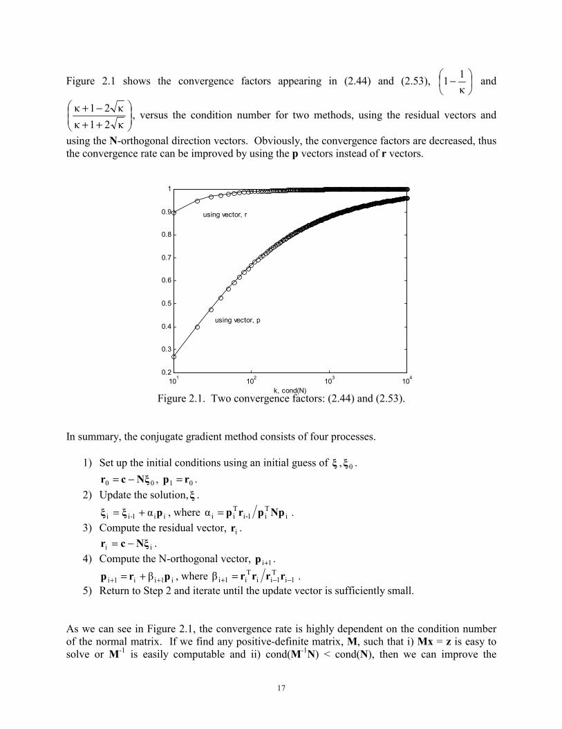
Figure 2.1 shows the convergence factors appearing in (2.44) and (2.53),

−

κ11 and

++−+

κ21κκ21κ , versus the condition number for two methods, using the residual vectors and

using the N-orthogonal direction vectors. Obviously, the convergence factors are decreased, thus the convergence rate can be improved by using the p vectors instead of r vectors.

101 102 103 1040.2

0.3

0.4

0.5

0.6

0.7

0.8

0.9

1

k, cond(N)

using vector, r

using vector, p

Figure 2.1. Two convergence factors: (2.44) and (2.53).

In summary, the conjugate gradient method consists of four processes.

1) Set up the initial conditions using an initial guess of ξ , 0ξ .

0100 , rpNξcr =−= . 2) Update the solution,ξ .

ii1-ii α pξξ += , where iTi1-i

Tiiα Npprp= .

3) Compute the residual vector, ir .

ii Nξcr −= . 4) Compute the N-orthogonal vector, 1i+p .

i1ii1i β prp ++ += , where 1iT

1iiTi1iβ −−+ = rrrr .

5) Return to Step 2 and iterate until the update vector is sufficiently small. As we can see in Figure 2.1, the convergence rate is highly dependent on the condition number of the normal matrix. If we find any positive-definite matrix, M, such that i) Mx = z is easy to solve or M-1 is easily computable and ii) cond(M-1N) < cond(N), then we can improve the

18

convergence rate once again. Therefore, the iteration can be reduced by preconditioning the original linear system of equations with the easily computable matrix, M. Assume that M-1 is already found. The original linear system is converted to the following linear system.

cξN ~ˆ~ = , (2.54) where NMN 1~ −= and cMc 1~ −= . The condition number of the modified normal matrix should be smaller than that of the original normal matrix. The factor of (2.53), therefore, will be decreased and the convergence rate will be increased.

Again, the normal matrix, N, is not computed explicitly because it needs matrix-matrix multiplication (N=ATA), which requires extremely demanding costs. Instead, the effect of the normal matrix is computed by calculating two matrix-vector multiplications (a=Ap and q=ATa), which is almost nothing comparing to the matrix-matrix multiplication. In our computation, there are three matrix-vector multiplications (one in Step 2 and two in Step 3, ~O(2nm+m2) flops) and two vector-vector multiplications (two in Step 2, ~O(2m) flops) per iteration. The preconditioning matrix, M, is chosen as the block-diagonal part of the matrix, N, because N is block-diagonally dominant and M is quickly computable with limited memory storage. The multiplication of the preconditioner, M-1 is also a less costly job because the preconditioner is a very sparse matrix having non-zeroes only in a very narrow block-diagonal part.

19

3. GLOBAL GRAVITY FIELD RECOVERY USING IN SITU POTENTIAL OBSERVABLE FROM CHAMP

3.1. Introduction Since its launch in July 2000, the GeoForschungsZentrum Potsdam (GFZ) CHAllenging Minisatellite Payload (CHAMP) gravity and magnetic mapping satellite mission has been providing invaluable data for gravity field studies. CHAMP’s orbit is at a low altitude of 450 km and its 870 inclination enables near-global sampling. Its payload includes geodetic quality GPS receivers (Blackjack-class, 16-channel, dual-frequency) with multiple antennas for precise orbit determination and atmospheric limb-sounding, and the 3-axis STAR accelerometer (3x10-9 m/s2 and 3x10-8 m/s2 precision in the along track or cross track, and radial directions, respectively) [Perett et al., 2001] to measure non-conservative forces including atmospheric drag. The CHAMP accelerometer has been performing well except in the radial component (x-axis), that provides unrealistically large accelerations [CHAMP newsletter No.4, 2001]; however, a correction of this problem is anticipated [Ch. Reigber and R. Biancale, 2002, personal communications]. The CHAMP Project at GFZ Potsdam provides a Rapid Science Orbit (RSO) with 30-second sampling and processed accelerometer data every 10 seconds [GFZ CHAMP Project, 2002]. Recently, a number of CHAMP precise orbit data products, e.g., Rim et al. [2001], and accuracy evaluations of these orbits have become available, [H. Boomkamp and J. Dow, 2002, personal communications, http://nng.esoc.esa.de/gps/campaign.html]. The conventional technique for gravity field solutions using satellite tracking data involves a geophysical inversion process that relates the data (e.g., high-low GPS phase tracking data) to the geopotential field represented in spherical harmonics and estimates its coefficients using a rigorous inversion [e.g., EGM96, Lemoine et al., 1998; GRIM5C1, Gruber et al., 2000]. In this study, it is intended to demonstrate a more simple (straightforward) technique based on the method by Jekeli [1999] that uses precise orbits (RSO) in the inertial frame and the conservation of energy principle, to construct on-orbit disturbing potential observations from the CHAMP data only in the along track component. The first resulting gravity field solution, OSU02A, using only 16-days of CHAMP data is complete to degree and order 50. OSU02A is then compared and evaluated against EGM96, GRIM5C1, and the more recent solutions, EIGEN1S (a satellite-only model including 88-days of CHAMP data [Reigber et al, 2002]) and TEG4 (a combination model including 80-days of CHAMP data [Tapley et al., 2002]). The models are also evaluated using independent Arctic gravity anomaly data and GPS/leveling data. Besides RSO, there are other sample orbit products available as contributions of CHAMP orbit campaign [CDDISA, 2002]. 11 days of dynamic orbits, reduced-dynamic orbits, and kinematic orbits are provided by diverse agencies and universities including CSR, JPL, GFZ, and so on. Two dynamic orbits based on different a priori gravity fields from CSR and GFZ, a reduced-dynamic orbit from JPL, and a kinematic orbit from ESA, are used to compute the in situ potentials. From the potential measurements, the corresponding global gravity fields (some variants of OSU02A) are recovered up to degree and order 50 with the accelerometer data from GFZ. The recovered gravity solutions are compared with other previous gravity models and assessed with the independent gravity anomaly data.

In order to use the accelerometer data to compute the dissipating energy, it is necessary to calibrate the raw accelerometer measurements by estimating the scale factor, the bias, and its possible drift parameters. It will be discussed how large their effects are in terms of the potential

20

values and how the accelerometer data can be calibrated with respect to a reference gravity field. Only the along-track component was used for this study, because the other components are less dominant (one order of magnitude smaller) and it is a second-order effect in the energy computation. To mitigate the unmodeled forces such as the remaining tidal forces and the empirical forces such as the once-per-revolution effect existing in the CHAMP orbit data, some non-gravitational parameters were modeled and estimated prior to the geopotential determination. The results on the accelerometer calibration and non-gravitational (empirical) force estimation are shown in this Chapter.

The solution method is based on the conjugate gradient with a preconditioner, which was already introduced in Chapter 2. This method is applied to estimate the geopotential coefficients iteratively and efficiently. The (true and approximate) error covariances of the estimated coefficients are computed as well. It will be presented how good and efficient the approximate error covariance is compared to the true one.

At present, the temporal variations of the Earth’s gravity field are available only from the analysis of satellite laser ranging (SLR) data for many years. The maximum degree and order is limited up to 4. The CHAMP mission can provide potentially very good insight of the time variation of the Earth gravity field. Currently, GFZ provides about 2 years of almost continuous high-low CHAMP data. Using these, the monthly mean gravity fields are estimated up to degree and order 70 for almost 1.5 years covering 2 years of period. The temporal variations of low degree geopotential coefficients are obtained from the time series of CHAMP solutions, and they are compared with the SLR derived solutions. 3.2. Observation equation In Chapter 2, we derived an accurate model relating the Earth’s gravitational potential, VE, to x, x& , and F in the inertial frame, where x is the position vector, x& is the velocity vector, and F designates the net force vector including all non-conservative forces measured by the accelerometer:

( ) 0Tii

1i2

i2

i1e

2iE VVdtxxxxω

21V −−⋅−−−= ∫ xFx &&&& . (3.1)

where eω is the Earth’s rotation rate, Ti

3i2

i1

i ][ xxx=x and Ti3

i2

i1

i ][ xxx &&&& =x . The harmonic geopotential coefficients can be estimated from a global distribution of observable, VE. For this derivation, the luni-solar gravitational potential, VS+VM, is the only N-Body effect considered. The N-body effect, for example, could be accurately modeled using a planetary ephemeris, such as JPL DE405. The first term in (3.1) is the kinetic energy (per unit mass) of the satellite, determined by its inertial velocity. The second term is the so-called ‘potential rotation’ term that accounts for the (dominant) rotation of the Earth’s potential in the inertial frame. The third term is the dissipating energy due to the atmospheric drag, solar radiation pressure, thermal forces, and other non-conservative forces. VT is the temporal variation of the gravitational potential due to the solid Earth tide, ocean tide, and the atmosphere and hydrology. The last term is the energy constant of the system including the constant zero-degree harmonic of the gravitational potential.

The in situ potential observation error and the corresponding height anomaly error due to the velocity and position measurements error are approximately obtained from considering the first and second terms of (3.1).

21

( ),δδωδννδV iiii

eE xxxx && ++⋅≤ (3.2)

where v and δv are the satellite speed and its error, and δV, iδx& , and iδx are errors in the

potential, velocity, and position, respectively. Usually, ix is O(107m), v is O(104m/s), and eω

is (10-4 rad/s). Assuming iδx is O(10-2m) and δv ≈ iδx& is O(10-5m/s), we find that the first

term is one order magnitude larger than the second term. It shows that the potential error is mostly and directly related to the velocity error of the low-Earth orbiting satellite. For example, we need the velocity as accurate as about 10 µm/s in order to get the potential observation accurate to 10-1 m2/s2. The corresponding in situ height anomaly error is obtained simply by dividing the in situ potential error by the normal gravity that is about 8.5 m/s2 at the altitude of the low Earth orbiting satellite. Therefore, we can expect 1 cm accuracy in the height anomaly from the above example.

In this study, the second-order gravitational sources such as the solid Earth and ocean tides are ignored, but the effect of the permanent tides is corrected. Although there are recently available precise orbits, the Rapid Science Orbit (RSO) is used, since it is accurate to approximately 4 cm radially (RMS) based on evaluations including the high-elevation satellite laser ranging (SLR) test [H. Rim, personal communications, 2002; http://nng.esoc.esa.de/gps/campaign.html]. 3.2.1 Scale, bias and bias drift in accelerometer data The STAR accelerometer assembly on board CHAMP measures the non-conservative forces in three dimensions. Its x-axis is aligned along the radial direction, the y-axis is along the direction of the forward boom, and the z-axis is along the (positive) perpendicular direction of the orbital plane. However, data from only the y-axis (along track) component are used in this study, primarily because it is the dominant component in the potential computation. In addition, the x-axis sensor is less sensitive and one component used to compute x-axis acceleration was discovered to have a malfunction [CHAMP newsletter No.4, 2001]. Thus, because also the boom direction component of the velocity vector dominates the total speed of the satellite (order of magnitude larger than other components), we have the following approximate friction energy formula:

δt)t(v)t(FdtV i

n

1iiy

iF ∑∫

=≈⋅= xF & . (3.3)

Instead of using the CHAMP stellar compass data to determine the precise component, Fy, we rely on the on-orbit stabilization of the satellite, which maintains the y-axis (forward boom) in the direction of the velocity. Thus, the energy dissipation term would be computed by approximating the inner product by the scalar multiplication of the only along-track component (i.e., y-axis) of the specific force measurements, yF , and the speed of the satellite, v .

The y-axis accelerometer data in GFZ’s level-2 products are not calibrated, which requires that the scale factor, bias, and drift be estimated or modeled. The raw accelerometer

22

measurements, STARyF , (again, only y-axis component) for the dissipating energy computation,

can be modeled with the scale factor, s , the bias, yδf , and the bias drift, yfδ& as follows:

( ),ttfδδfFsF 0yySTARyy −++⋅= & (3.4)

where t0 is the initial time and t is the epoch for the calibrated measurement, yF . Then, the dissipating (friction) energy, FV , is computed using the calibrated accelerometer data as follows:

( )( )

( ) dt.vttfδdtvδfdtvFs

dt,vttfδδfFs

dt,vF)t(V)t(V

t

ty0y

t

ty

t

ty

STARy

t

ty0yy

STARy

t

tyy0FF

000

0

0

∫∫∫

∫

∫

−++=

−++⋅=

≈−

&

& (3.5)

The quantities outside the integrals of the right-hand side are the unknown parameters, scale factor, bias, and bias drift, to be determined. Note that the along-track velocity is approximately constant and the second and third integrals turn out to be linear and quadratic functions over time, respectively. Therefore, the non-zero bias and bias drift in the accelerometer data tend to make a linear and a quadratic error in the dissipating energy computation, respectively. The integrals of the right-hand side are computable from the velocity and accelerometer measurements. It is required to obtain the left-hand side term in order to solve for three unknown parameters in the least-squares sense. The prior gravity model and the orbit data can be used to compute the left-hand side term. From equation (3.1), the friction energy,

dtV iF xf &⋅= ∫ , can be computed, assuming VE is known from an a priori gravity model. This

indicates that the dissipating energy computed from the accelerometer data will be fitted or adjusted to the dissipating energy derived from the prior gravity model by estimating three accelerometer calibration parameters; s, yδf , and yfδ& . In this paper, EGM96 model with the maximum degree and order of 70 is used to compute the left-hand side. Actually, the specific forces are caused by the non-gravitational forces acting on the satellite and the calibration of their measurements is not too sensitive to the gravitation model. Other gravity models were tested as well and do not provide significantly different estimates for the calibration parameters. In this study, the scale factor is fixed to the single global value from CSR [Tapley et al., 2002] and the biases and bias drifts are solved every day. 3.2.2 Empirical forces in orbit data The kinetic energy (and potential rotation) in equation (3.1) computed from orbit data may have significant systematic errors, which have the dominant period of once per revolution and twice per revolution. They may stem from the unmodeled temporal gravitational forces like the solid

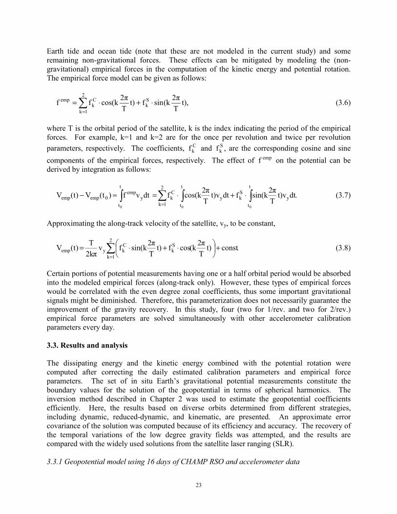
23

Earth tide and ocean tide (note that these are not modeled in the current study) and some remaining non-gravitational forces. These effects can be mitigated by modeling the (non-gravitational) empirical forces in the computation of the kinetic energy and potential rotation. The empirical force model can be given as follows:

,t)T2π(ksinft)

T2πcos(kff

2

1k

Sk

Ck

emp ∑=

⋅+⋅= (3.6)

where T is the orbital period of the satellite, k is the index indicating the period of the empirical forces. For example, k=1 and k=2 are for the once per revolution and twice per revolution parameters, respectively. The coefficients, C

kf and Skf , are the corresponding cosine and sine

components of the empirical forces, respectively. The effect of empf on the potential can be derived by integration as follows:

.dtt)vT2πsin(kfdtt)v

T2πcos(kfdt vf)t(V)t(V

2

1k

t

ty

Sk

t

ty

Ck

t

ty

emp0empemp

000

∑ ∫∫∫=

⋅+⋅=≈− (3.7)

Approximating the along-track velocity of the satellite, vy, to be constant,

.constt)T2π(kcosft)

T2πsin(kfv

2kπT )t(V

2

1k

Sk

Ckyemp ∑

=+

⋅+⋅= (3.8)

Certain portions of potential measurements having one or a half orbital period would be absorbed into the modeled empirical forces (along-track only). However, these types of empirical forces would be correlated with the even degree zonal coefficients, thus some important gravitational signals might be diminished. Therefore, this parameterization does not necessarily guarantee the improvement of the gravity recovery. In this study, four (two for 1/rev. and two for 2/rev.) empirical force parameters are solved simultaneously with other accelerometer calibration parameters every day. 3.3. Results and analysis The dissipating energy and the kinetic energy combined with the potential rotation were computed after correcting the daily estimated calibration parameters and empirical force parameters. The set of in situ Earth’s gravitational potential measurements constitute the boundary values for the solution of the geopotential in terms of spherical harmonics. The inversion method described in Chapter 2 was used to estimate the geopotential coefficients efficiently. Here, the results based on diverse orbits determined from different strategies, including dynamic, reduced-dynamic, and kinematic, are presented. An approximate error covariance of the solution was computed because of its efficiency and accuracy. The recovery of the temporal variations of the low degree gravity fields was attempted, and the results are compared with the widely used solutions from the satellite laser ranging (SLR). 3.3.1 Geopotential model using 16 days of CHAMP RSO and accelerometer data

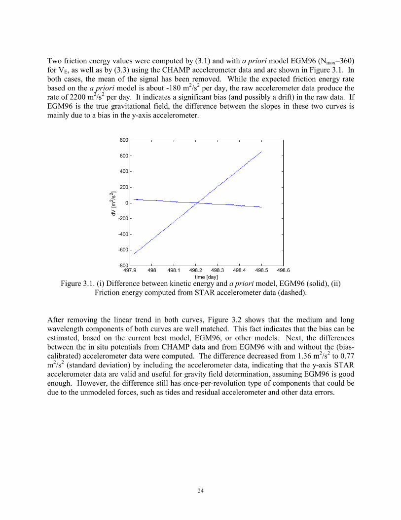
24

Two friction energy values were computed by (3.1) and with a priori model EGM96 (Nmax=360) for VE, as well as by (3.3) using the CHAMP accelerometer data and are shown in Figure 3.1. In both cases, the mean of the signal has been removed. While the expected friction energy rate based on the a priori model is about -180 m2/s2 per day, the raw accelerometer data produce the rate of 2200 m2/s2 per day. It indicates a significant bias (and possibly a drift) in the raw data. If EGM96 is the true gravitational field, the difference between the slopes in these two curves is mainly due to a bias in the y-axis accelerometer.

497.9 498 498.1 498.2 498.3 498.4 498.5 498.6-800

-600

-400

-200

0

200

400

600

800

time [day]

dV [m

2 /s2 ]

Figure 3.1. (i) Difference between kinetic energy and a priori model, EGM96 (solid), (ii)

Friction energy computed from STAR accelerometer data (dashed). After removing the linear trend in both curves, Figure 3.2 shows that the medium and long wavelength components of both curves are well matched. This fact indicates that the bias can be estimated, based on the current best model, EGM96, or other models. Next, the differences between the in situ potentials from CHAMP data and from EGM96 with and without the (bias-calibrated) accelerometer data were computed. The difference decreased from 1.36 m2/s2 to 0.77 m2/s2 (standard deviation) by including the accelerometer data, indicating that the y-axis STAR accelerometer data are valid and useful for gravity field determination, assuming EGM96 is good enough. However, the difference still has once-per-revolution type of components that could be due to the unmodeled forces, such as tides and residual accelerometer and other data errors.

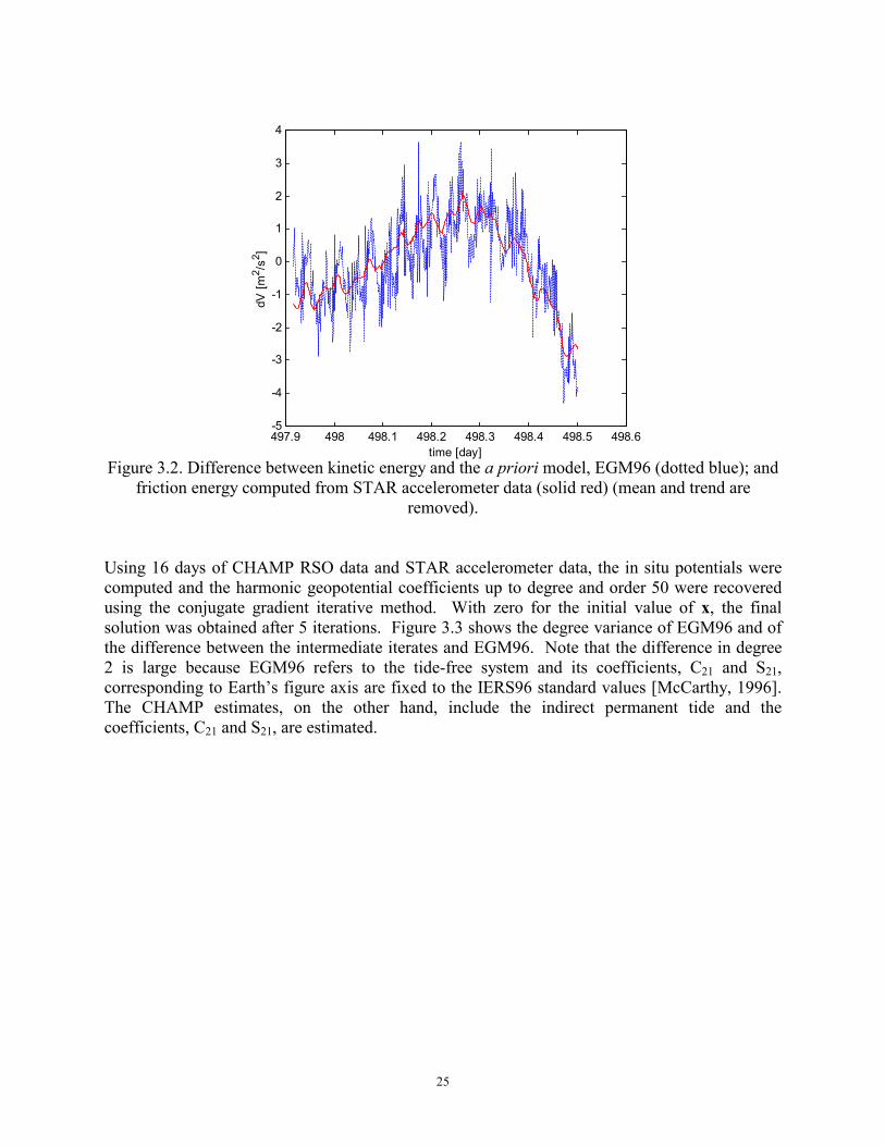
25

497.9 498 498.1 498.2 498.3 498.4 498.5 498.6-5

-4

-3

-2

-1

0

1

2

3

4

time [day]

dV [m

2 /s2 ]

Figure 3.2. Difference between kinetic energy and the a priori model, EGM96 (dotted blue); and

friction energy computed from STAR accelerometer data (solid red) (mean and trend are removed).

Using 16 days of CHAMP RSO data and STAR accelerometer data, the in situ potentials were computed and the harmonic geopotential coefficients up to degree and order 50 were recovered using the conjugate gradient iterative method. With zero for the initial value of x, the final solution was obtained after 5 iterations. Figure 3.3 shows the degree variance of EGM96 and of the difference between the intermediate iterates and EGM96. Note that the difference in degree 2 is large because EGM96 refers to the tide-free system and its coefficients, C21 and S21, corresponding to Earth’s figure axis are fixed to the IERS96 standard values [McCarthy, 1996]. The CHAMP estimates, on the other hand, include the indirect permanent tide and the coefficients, C21 and S21, are estimated.

26

0 10 20 30 40 50 10 -10

10 -8

10 -6

10 -4

10 -2

degree

degr

ee v

aria

nces

1st

2nd

3rd 4th & 5th

Figure 3.3. Degree variance of EGM96 signal (solid black) and difference between intermediate

iterations and EGM96. For consistency with other models such as EGM96 and TEG4, the solution adopts the C21 and S21 values according to the IERS2000 Standard [McCarthy, 2000] and the indirect permanent tide in the estimate, C20, is consistently handled as specified by the IERS2000 Standard. The recovered CHAMP gravity model (called OSU02A model) is compared with other recent gravity models. Figure 3.4 presents the degree variances of the differences among various pairs of gravity models. The GRIM5C1 model is closest to OSU02A, probably due to the fact that the CHAMP RSO is a dynamic orbit computed using GRIM5C1 model and CHAMP GPS and satellite laser ranging (SLR) tracking data. As the degree increases, the difference between GRIM5C1 and OSU02A gradually approaches the differences between other models and OSU02A. From degrees 43 to 50, the differences between OSU02A and GRIM5C1, EGM96, and TEG4, respectively, are almost identical. Whereas the latter three models are based on satellite tracking as well as terrestrial gravity data, the satellite-only model, EIGEN1S, combined 88 days of CHAMP data with satellite laser ranging data, and is based on the GRIM5S1 normal equation system [Reigber et al, 2002]. The OSU02A differences relative to EIGEN1S are similar with those of EGM96 and TEG4 below degree 35, however, they become relatively larger beyond degree 35. The fact that OSU02A follows the models GRIM5C1, EGM96, and TEG4 more closely than EIGEN1S beyond degrees 35, indicates that RSO and consequently OSU02A is significantly affected by terrestrial data.

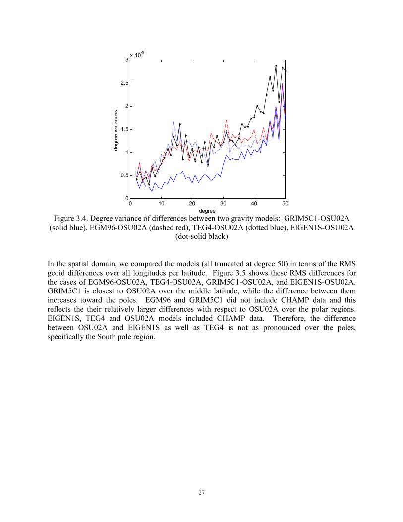
27

0 10 20 30 40 500

0.5

1

1.5

2

2.5

3x 10-9

degree

degr

ee v

aria

nces

Figure 3.4. Degree variance of differences between two gravity models: GRIM5C1-OSU02A

(solid blue), EGM96-OSU02A (dashed red), TEG4-OSU02A (dotted blue), EIGEN1S-OSU02A (dot-solid black)

In the spatial domain, we compared the models (all truncated at degree 50) in terms of the RMS geoid differences over all longitudes per latitude. Figure 3.5 shows these RMS differences for the cases of EGM96-OSU02A, TEG4-OSU02A, GRIM5C1-OSU02A, and EIGEN1S-OSU02A. GRIM5C1 is closest to OSU02A over the middle latitude, while the difference between them increases toward the poles. EGM96 and GRIM5C1 did not include CHAMP data and this reflects the their relatively larger differences with respect to OSU02A over the polar regions. EIGEN1S, TEG4 and OSU02A models included CHAMP data. Therefore, the difference between OSU02A and EIGEN1S as well as TEG4 is not as pronounced over the poles, specifically the South pole region.

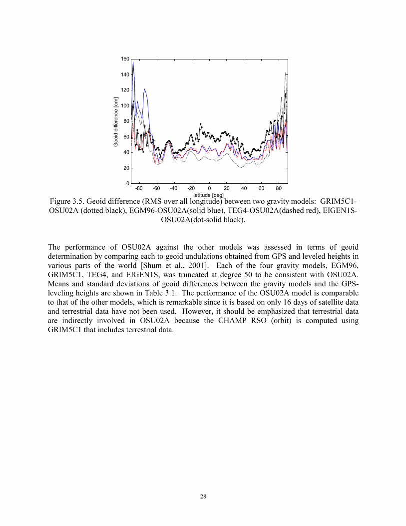
28

-80 -60 -40 -20 0 20 40 60 800

20

40

60

80

100

120

140

160

latitude [deg]

Geo

id d

iffer

ence

[cm

]

Figure 3.5. Geoid difference (RMS over all longitude) between two gravity models: GRIM5C1-OSU02A (dotted black), EGM96-OSU02A(solid blue), TEG4-OSU02A(dashed red), EIGEN1S-

OSU02A(dot-solid black). The performance of OSU02A against the other models was assessed in terms of geoid determination by comparing each to geoid undulations obtained from GPS and leveled heights in various parts of the world [Shum et al., 2001]. Each of the four gravity models, EGM96, GRIM5C1, TEG4, and EIGEN1S, was truncated at degree 50 to be consistent with OSU02A. Means and standard deviations of geoid differences between the gravity models and the GPS-leveling heights are shown in Table 3.1. The performance of the OSU02A model is comparable to that of the other models, which is remarkable since it is based on only 16 days of satellite data and terrestrial data have not been used. However, it should be emphasized that terrestrial data are indirectly involved in OSU02A because the CHAMP RSO (orbit) is computed using GRIM5C1 that includes terrestrial data.

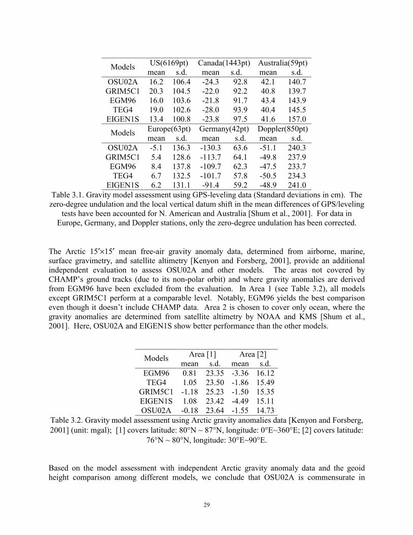
29

US(6169pt) Canada(1443pt) Australia(59pt) Models mean s.d. mean s.d. mean s.d.

OSU02A 16.2 106.4 -24.3 92.8 42.1 140.7 GRIM5C1 20.3 104.5 -22.0 92.2 40.8 139.7

EGM96 16.0 103.6 -21.8 91.7 43.4 143.9 TEG4 19.0 102.6 -28.0 93.9 40.4 145.5

EIGEN1S 13.4 100.8 -23.8 97.5 41.6 157.0 Europe(63pt) Germany(42pt) Doppler(850pt) Models mean s.d. mean s.d. mean s.d.

OSU02A -5.1 136.3 -130.3 63.6 -51.1 240.3 GRIM5C1 5.4 128.6 -113.7 64.1 -49.8 237.9

EGM96 8.4 137.8 -109.7 62.3 -47.5 233.7 TEG4 6.7 132.5 -101.7 57.8 -50.5 234.3

EIGEN1S 6.2 131.1 -91.4 59.2 -48.9 241.0 Table 3.1. Gravity model assessment using GPS-leveling data (Standard deviations in cm). The

zero-degree undulation and the local vertical datum shift in the mean differences of GPS/leveling tests have been accounted for N. American and Australia [Shum et al., 2001]. For data in

Europe, Germany, and Doppler stations, only the zero-degree undulation has been corrected. The Arctic 15′×15′ mean free-air gravity anomaly data, determined from airborne, marine, surface gravimetry, and satellite altimetry [Kenyon and Forsberg, 2001], provide an additional independent evaluation to assess OSU02A and other models. The areas not covered by CHAMP’s ground tracks (due to its non-polar orbit) and where gravity anomalies are derived from EGM96 have been excluded from the evaluation. In Area 1 (see Table 3.2), all models except GRIM5C1 perform at a comparable level. Notably, EGM96 yields the best comparison even though it doesn’t include CHAMP data. Area 2 is chosen to cover only ocean, where the gravity anomalies are determined from satellite altimetry by NOAA and KMS [Shum et al., 2001]. Here, OSU02A and EIGEN1S show better performance than the other models.

Area [1] Area [2] Models mean s.d. mean s.d. EGM96 0.81 23.35 -3.36 16.12TEG4 1.05 23.50 -1.86 15.49

GRIM5C1 -1.18 25.23 -1.50 15.35EIGEN1S 1.08 23.42 -4.49 15.11OSU02A -0.18 23.64 -1.55 14.73

Table 3.2. Gravity model assessment using Arctic gravity anomalies data [Kenyon and Forsberg, 2001] (unit: mgal); [1] covers latitude: 80°N ~ 87°N, longitude: 0°E~360°E; [2] covers latitude:

76°N ~ 80°N, longitude: 30°E~90°E. Based on the model assessment with independent Arctic gravity anomaly data and the geoid height comparison among different models, we conclude that OSU02A is commensurate in

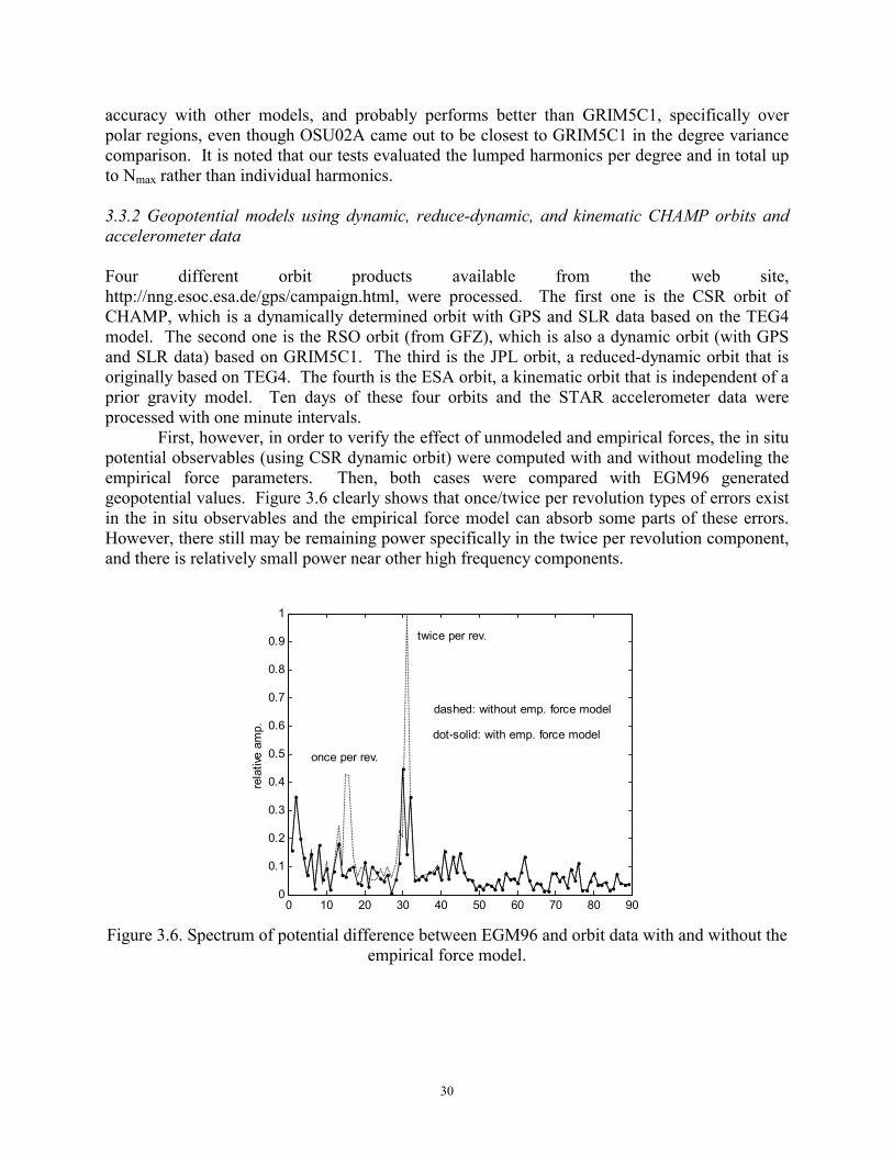
30

accuracy with other models, and probably performs better than GRIM5C1, specifically over polar regions, even though OSU02A came out to be closest to GRIM5C1 in the degree variance comparison. It is noted that our tests evaluated the lumped harmonics per degree and in total up to Nmax rather than individual harmonics. 3.3.2 Geopotential models using dynamic, reduce-dynamic, and kinematic CHAMP orbits and accelerometer data Four different orbit products available from the web site, http://nng.esoc.esa.de/gps/campaign.html, were processed. The first one is the CSR orbit of CHAMP, which is a dynamically determined orbit with GPS and SLR data based on the TEG4 model. The second one is the RSO orbit (from GFZ), which is also a dynamic orbit (with GPS and SLR data) based on GRIM5C1. The third is the JPL orbit, a reduced-dynamic orbit that is originally based on TEG4. The fourth is the ESA orbit, a kinematic orbit that is independent of a prior gravity model. Ten days of these four orbits and the STAR accelerometer data were processed with one minute intervals.

First, however, in order to verify the effect of unmodeled and empirical forces, the in situ potential observables (using CSR dynamic orbit) were computed with and without modeling the empirical force parameters. Then, both cases were compared with EGM96 generated geopotential values. Figure 3.6 clearly shows that once/twice per revolution types of errors exist in the in situ observables and the empirical force model can absorb some parts of these errors. However, there still may be remaining power specifically in the twice per revolution component, and there is relatively small power near other high frequency components.

0 10 20 30 40 50 60 70 80 900

0.1

0.2

0.3

0.4

0.5

0.6

0.7

0.8

0.9

1

rela

tive

amp.

once per rev.

twice per rev.

dashed: without emp. force model

dot-solid: with emp. force model

Figure 3.6. Spectrum of potential difference between EGM96 and orbit data with and without the

empirical force model.

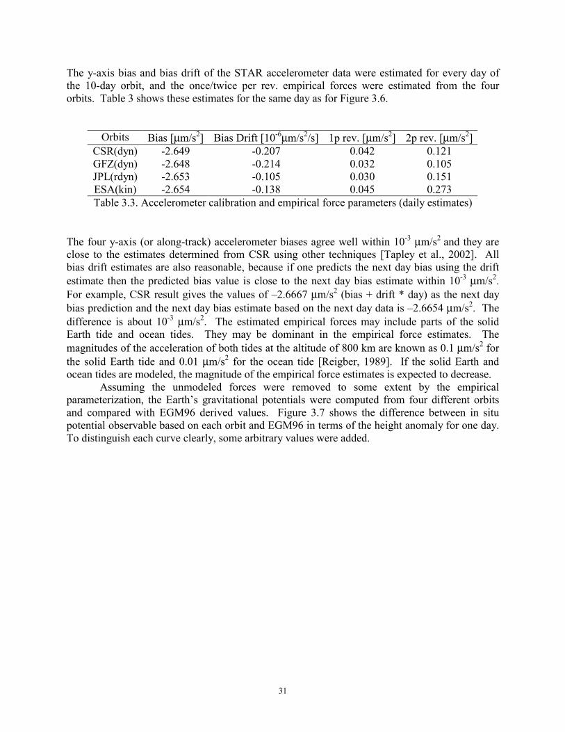
31

The y-axis bias and bias drift of the STAR accelerometer data were estimated for every day of the 10-day orbit, and the once/twice per rev. empirical forces were estimated from the four orbits. Table 3 shows these estimates for the same day as for Figure 3.6.

Orbits Bias [µm/s2] Bias Drift [10-6µm/s2/s] 1p rev. [µm/s2] 2p rev. [µm/s2]CSR(dyn) -2.649 -0.207 0.042 0.121 GFZ(dyn) -2.648 -0.214 0.032 0.105 JPL(rdyn) -2.653 -0.105 0.030 0.151 ESA(kin) -2.654 -0.138 0.045 0.273 Table 3.3. Accelerometer calibration and empirical force parameters (daily estimates)

The four y-axis (or along-track) accelerometer biases agree well within 10-3 µm/s2 and they are close to the estimates determined from CSR using other techniques [Tapley et al., 2002]. All bias drift estimates are also reasonable, because if one predicts the next day bias using the drift estimate then the predicted bias value is close to the next day bias estimate within 10-3 µm/s2. For example, CSR result gives the values of –2.6667 µm/s2 (bias + drift * day) as the next day bias prediction and the next day bias estimate based on the next day data is –2.6654 µm/s2. The difference is about 10-3 µm/s2. The estimated empirical forces may include parts of the solid Earth tide and ocean tides. They may be dominant in the empirical force estimates. The magnitudes of the acceleration of both tides at the altitude of 800 km are known as 0.1 µm/s2 for the solid Earth tide and 0.01 µm/s2 for the ocean tide [Reigber, 1989]. If the solid Earth and ocean tides are modeled, the magnitude of the empirical force estimates is expected to decrease.

Assuming the unmodeled forces were removed to some extent by the empirical parameterization, the Earth’s gravitational potentials were computed from four different orbits and compared with EGM96 derived values. Figure 3.7 shows the difference between in situ potential observable based on each orbit and EGM96 in terms of the height anomaly for one day. To distinguish each curve clearly, some arbitrary values were added.

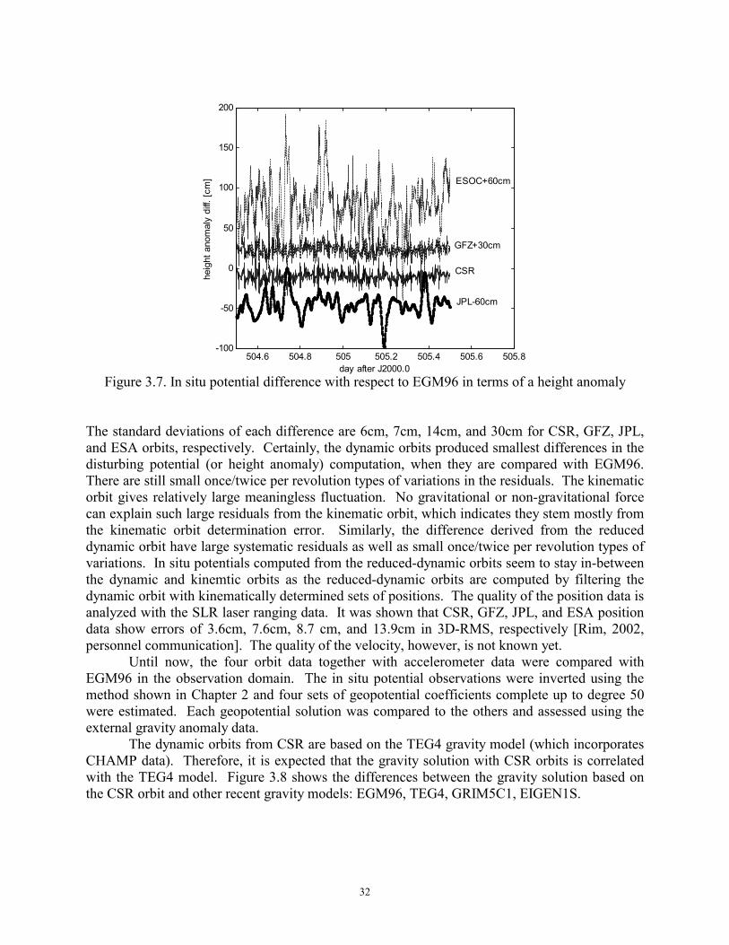
32

504.6 504.8 505 505.2 505.4 505.6 505.8-100

-50

0

50

100

150

200

day after J2000.0

heig

ht a

nom

aly

diff.

[cm

]

CSR

GFZ+30cm

JPL-60cm

ESOC+60cm

Figure 3.7. In situ potential difference with respect to EGM96 in terms of a height anomaly

The standard deviations of each difference are 6cm, 7cm, 14cm, and 30cm for CSR, GFZ, JPL, and ESA orbits, respectively. Certainly, the dynamic orbits produced smallest differences in the disturbing potential (or height anomaly) computation, when they are compared with EGM96. There are still small once/twice per revolution types of variations in the residuals. The kinematic orbit gives relatively large meaningless fluctuation. No gravitational or non-gravitational force can explain such large residuals from the kinematic orbit, which indicates they stem mostly from the kinematic orbit determination error. Similarly, the difference derived from the reduced dynamic orbit have large systematic residuals as well as small once/twice per revolution types of variations. In situ potentials computed from the reduced-dynamic orbits seem to stay in-between the dynamic and kinemtic orbits as the reduced-dynamic orbits are computed by filtering the dynamic orbit with kinematically determined sets of positions. The quality of the position data is analyzed with the SLR laser ranging data. It was shown that CSR, GFZ, JPL, and ESA position data show errors of 3.6cm, 7.6cm, 8.7 cm, and 13.9cm in 3D-RMS, respectively [Rim, 2002, personnel communication]. The quality of the velocity, however, is not known yet. Until now, the four orbit data together with accelerometer data were compared with EGM96 in the observation domain. The in situ potential observations were inverted using the method shown in Chapter 2 and four sets of geopotential coefficients complete up to degree 50 were estimated. Each geopotential solution was compared to the others and assessed using the external gravity anomaly data. The dynamic orbits from CSR are based on the TEG4 gravity model (which incorporates CHAMP data). Therefore, it is expected that the gravity solution with CSR orbits is correlated with the TEG4 model. Figure 3.8 shows the differences between the gravity solution based on the CSR orbit and other recent gravity models: EGM96, TEG4, GRIM5C1, EIGEN1S.

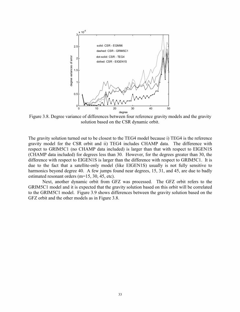
33

0 10 20 30 40 500

0.5

1

1.5

2

2.5

3x 10-8

degree

degr

ee v

aria

nces

of e

rror

solid: CSR - EGM96

dashed: CSR - GRIM5C1

dot-solid: CSR - TEG4

dotted: CSR - EIGEN1S

Figure 3.8. Degree variance of differences between four reference gravity models and the gravity

solution based on the CSR dynamic orbit. The gravity solution turned out to be closest to the TEG4 model because i) TEG4 is the reference gravity model for the CSR orbit and ii) TEG4 includes CHAMP data. The difference with respect to GRIM5C1 (no CHAMP data included) is larger than that with respect to EIGEN1S (CHAMP data included) for degrees less than 30. However, for the degrees greater than 30, the difference with respect to EIGEN1S is larger than the difference with respect to GRIM5C1. It is due to the fact that a satellite-only model (like EIGEN1S) usually is not fully sensitive to harmonics beyond degree 40. A few jumps found near degrees, 15, 31, and 45, are due to badly estimated resonant orders (m=15, 30, 45, etc). Next, another dynamic orbit from GFZ was processed. The GFZ orbit refers to the GRIM5C1 model and it is expected that the gravity solution based on this orbit will be correlated to the GRIM5C1 model. Figure 3.9 shows differences between the gravity solution based on the GFZ orbit and the other models as in Figure 3.8.

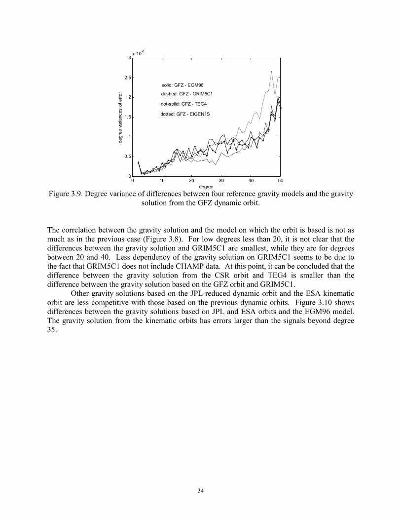
34

0 10 20 30 40 500

0.5

1

1.5

2

2.5

3x 10-8

degree

degr

ee v

aria

nces

of e

rror

solid: GFZ - EGM96

dashed: GFZ - GRIM5C1

dot-solid: GFZ - TEG4

dotted: GFZ - EIGEN1S

Figure 3.9. Degree variance of differences between four reference gravity models and the gravity

solution from the GFZ dynamic orbit. The correlation between the gravity solution and the model on which the orbit is based is not as much as in the previous case (Figure 3.8). For low degrees less than 20, it is not clear that the differences between the gravity solution and GRIM5C1 are smallest, while they are for degrees between 20 and 40. Less dependency of the gravity solution on GRIM5C1 seems to be due to the fact that GRIM5C1 does not include CHAMP data. At this point, it can be concluded that the difference between the gravity solution from the CSR orbit and TEG4 is smaller than the difference between the gravity solution based on the GFZ orbit and GRIM5C1. Other gravity solutions based on the JPL reduced dynamic orbit and the ESA kinematic orbit are less competitive with those based on the previous dynamic orbits. Figure 3.10 shows differences between the gravity solutions based on JPL and ESA orbits and the EGM96 model. The gravity solution from the kinematic orbits has errors larger than the signals beyond degree 35.

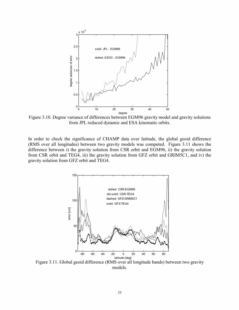
35

0 10 20 30 40 500

0.5

1

1.5

2

2.5

3x 10

-8

degree

degr

ee v

aria

nces

of e

rror

solid: JPL - EGM96

dotted: ESOC - EGM96

Figure 3.10. Degree variance of differences between EGM96 gravity model and gravity solutions

from JPL reduced dynamic and ESA kinematic orbits. In order to check the significance of CHAMP data over latitude, the global geoid difference (RMS over all longitudes) between two gravity models was computed. Figure 3.11 shows the difference between i) the gravity solution from CSR orbit and EGM96, ii) the gravity solution from CSR orbit and TEG4, iii) the gravity solution from GFZ orbit and GRIM5C1, and iv) the gravity solution from GFZ orbit and TEG4.

-80 -60 -40 -20 0 20 40 60 800

50

100

150

dotted: CSR-EGM96dot-solid: CSR-TEG4dashed: GFZ-GRIM5C1

solid: GFZ-TEG4

latitude [deg]

erro

r [cm

]

Figure 3.11. Global geoid difference (RMS over all longitude bands) between two gravity

models.

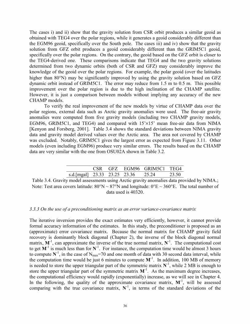
36

The cases i) and ii) show that the gravity solution from CSR orbit produces a similar geoid as obtained with TEG4 over the polar regions, while it generates a geoid considerably different than the EGM96 geoid, specifically over the South pole. The cases iii) and iv) show that the gravity solution from GFZ orbit produces a geoid considerably different than the GRIM5C1 geoid, specifically over the polar regions. On the contrary, the geoid based on the GFZ orbit is closer to the TEG4-derived one. These comparisons indicate that TEG4 and the two gravity solutions determined from two dynamic orbits (both of CSR and GFZ) may considerably improve the knowledge of the geoid over the polar regions. For example, the polar geoid (over the latitudes higher than 80°N) may be significantly improved by using the gravity solution based on GFZ dynamic orbit instead of GRIM5C1. The error may reduce from 1.5 m to 0.5 m. This possible improvement over the polar region is due to the high inclination of the CHAMP satellite. However, it is just a comparison between models without implying any accuracy of the new CHAMP models. To verify the real improvement of the new models by virtue of CHAMP data over the polar regions, external data such as Arctic gravity anomalies were used. The free-air gravity anomalies were computed from five gravity models (including two CHAMP gravity models, EGM96, GRIM5C1, and TEG4) and compared with 15’×15’ mean free-air data from NIMA [Kenyon and Forsberg, 2001]. Table 3.4 shows the standard deviations between NIMA gravity data and gravity model derived values over the Arctic area. The area not covered by CHAMP was excluded. Notably, GRIM5C1 gives the largest error as expected from Figure 3.11. Other models (even including EGM96) produce very similar errors. The results based on the CHAMP data are very similar with the one from OSU02A shown in Table 3.2.

CSR GFZ EGM96 GRIM5C1 TEG4 s.d.[mgal] 23.33 23.25 23.36 25.24 23.50

Table 3.4. Gravity model assessments using Arctic gravity anomalies data provided by NIMA.; Note: Test area covers latitude: 80°N ~ 87°N and longitude: 0°E ~ 360°E. The total number of

data used is 40320. 3.3.3 On the use of a preconditioning matrix as an error variance-covariance matrix The iterative inversion provides the exact estimates very efficiently, however, it cannot provide formal accuracy information of the estimates. In this study, the preconditioner is proposed as an (approximate) error covariance matrix. Because the normal matrix for CHAMP gravity field recovery is dominantly block diagonal (Chapter 2), the inverse of the block diagonal normal matrix, M-1, can approximate the inverse of the true normal matrix, N-1. The computational cost to get M-1 is much less than for N-1. For instance, the computation time would be almost 3 hours to compute N-1, in the case of Nmax=70 and one month of data with 30 second data interval, while the computation time would be just 6 minutes to compute M-1. In addition, 100 MB of memory is needed to store the upper triangular part of the symmetric matrix N-1, while 2 MB is enough to store the upper triangular part of the symmetric matrix M-1. As the maximum degree increases, the computational efficiency would rapidly (exponentially) increase, as we will see in Chapter 4. In the following, the quality of the approximate covariance matrix, M-1, will be assessed comparing with the true covariance matrix, N-1, in terms of the standard deviations of the

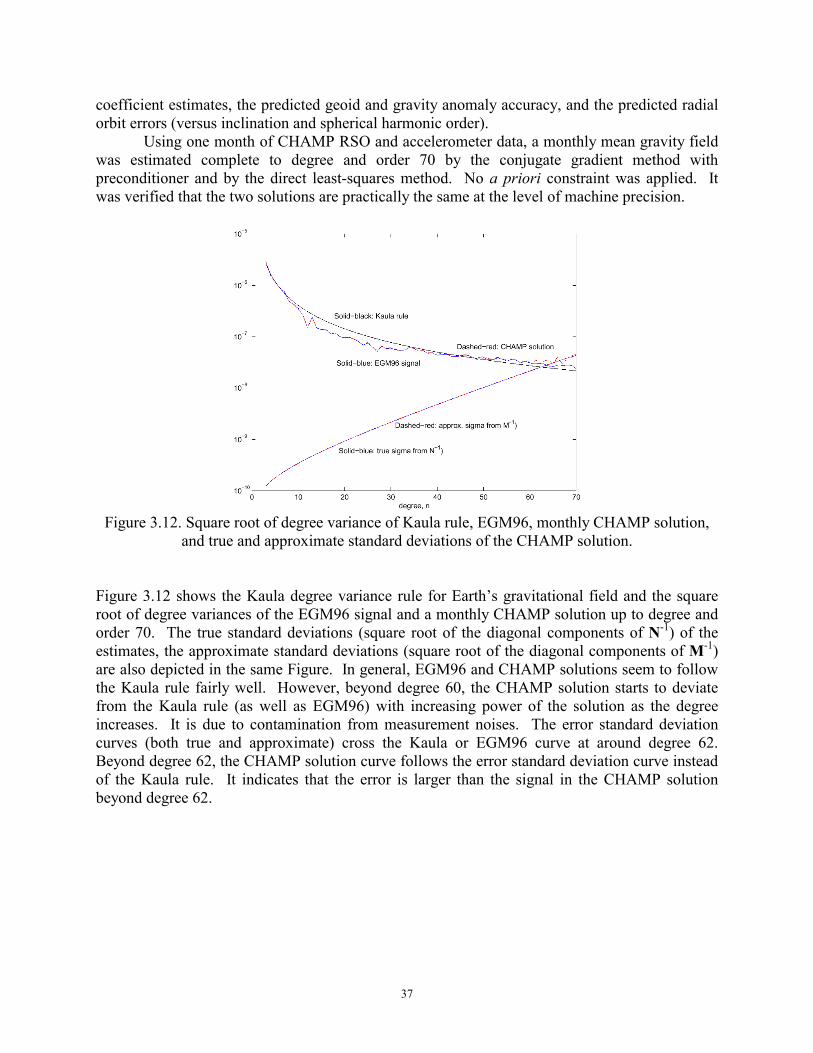
37

coefficient estimates, the predicted geoid and gravity anomaly accuracy, and the predicted radial orbit errors (versus inclination and spherical harmonic order).

Using one month of CHAMP RSO and accelerometer data, a monthly mean gravity field was estimated complete to degree and order 70 by the conjugate gradient method with preconditioner and by the direct least-squares method. No a priori constraint was applied. It was verified that the two solutions are practically the same at the level of machine precision.

Figure 3.12. Square root of degree variance of Kaula rule, EGM96, monthly CHAMP solution,

and true and approximate standard deviations of the CHAMP solution. Figure 3.12 shows the Kaula degree variance rule for Earth’s gravitational field and the square root of degree variances of the EGM96 signal and a monthly CHAMP solution up to degree and order 70. The true standard deviations (square root of the diagonal components of N-1) of the estimates, the approximate standard deviations (square root of the diagonal components of M-1) are also depicted in the same Figure. In general, EGM96 and CHAMP solutions seem to follow the Kaula rule fairly well. However, beyond degree 60, the CHAMP solution starts to deviate from the Kaula rule (as well as EGM96) with increasing power of the solution as the degree increases. It is due to contamination from measurement noises. The error standard deviation curves (both true and approximate) cross the Kaula or EGM96 curve at around degree 62. Beyond degree 62, the CHAMP solution curve follows the error standard deviation curve instead of the Kaula rule. It indicates that the error is larger than the signal in the CHAMP solution beyond degree 62.

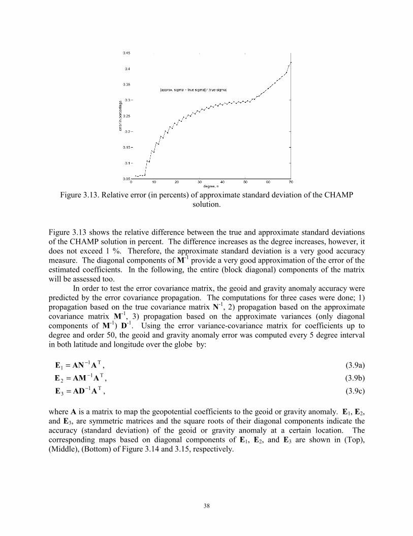
38

Figure 3.13. Relative error (in percents) of approximate standard deviation of the CHAMP

solution. Figure 3.13 shows the relative difference between the true and approximate standard deviations of the CHAMP solution in percent. The difference increases as the degree increases, however, it does not exceed 1 %. Therefore, the approximate standard deviation is a very good accuracy measure. The diagonal components of M-1 provide a very good approximation of the error of the estimated coefficients. In the following, the entire (block diagonal) components of the matrix will be assessed too. In order to test the error covariance matrix, the geoid and gravity anomaly accuracy were predicted by the error covariance propagation. The computations for three cases were done; 1) propagation based on the true covariance matrix N-1, 2) propagation based on the approximate covariance matrix M-1, 3) propagation based on the approximate variances (only diagonal components of M-1) D-1. Using the error variance-covariance matrix for coefficients up to degree and order 50, the geoid and gravity anomaly error was computed every 5 degree interval in both latitude and longitude over the globe by:

T11 AANE −= , (3.9a)

T12 AAME −= , (3.9b)

T13 AADE −= , (3.9c)

where A is a matrix to map the geopotential coefficients to the geoid or gravity anomaly. E1, E2, and E3, are symmetric matrices and the square roots of their diagonal components indicate the accuracy (standard deviation) of the geoid or gravity anomaly at a certain location. The corresponding maps based on diagonal components of E1, E2, and E3 are shown in (Top), (Middle), (Bottom) of Figure 3.14 and 3.15, respectively.

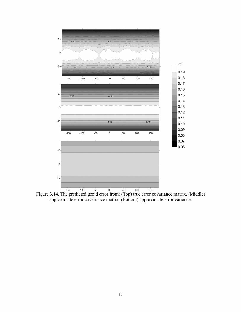
39

[m]

-150 -100 -50 0 50 100 150

-50

0

50

0.060.070.080.090.100.110.120.130.140.150.160.170.180.19

-150 -100 -50 0 50 100 150

-50

0

50

-150 -100 -50 0 50 100 150

-50

0

50

Figure 3.14. The predicted geoid error from; (Top) true error covariance matrix, (Middle)

approximate error covariance matrix, (Bottom) approximate error variance.

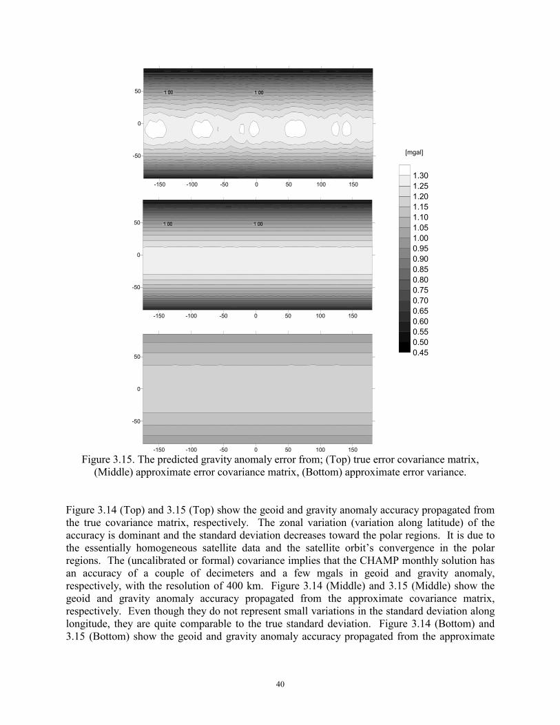
40

[mgal]

-150 -100 -50 0 50 100 150

-50

0

50

0.450.500.550.600.650.700.750.800.850.900.951.001.051.101.151.201.251.30

-150 -100 -50 0 50 100 150

-50

0

50

-150 -100 -50 0 50 100 150

-50

0

50

Figure 3.15. The predicted gravity anomaly error from; (Top) true error covariance matrix,

(Middle) approximate error covariance matrix, (Bottom) approximate error variance. Figure 3.14 (Top) and 3.15 (Top) show the geoid and gravity anomaly accuracy propagated from the true covariance matrix, respectively. The zonal variation (variation along latitude) of the accuracy is dominant and the standard deviation decreases toward the polar regions. It is due to the essentially homogeneous satellite data and the satellite orbit’s convergence in the polar regions. The (uncalibrated or formal) covariance implies that the CHAMP monthly solution has an accuracy of a couple of decimeters and a few mgals in geoid and gravity anomaly, respectively, with the resolution of 400 km. Figure 3.14 (Middle) and 3.15 (Middle) show the geoid and gravity anomaly accuracy propagated from the approximate covariance matrix, respectively. Even though they do not represent small variations in the standard deviation along longitude, they are quite comparable to the true standard deviation. Figure 3.14 (Bottom) and 3.15 (Bottom) show the geoid and gravity anomaly accuracy propagated from the approximate

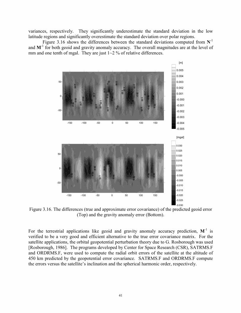
41

variances, respectively. They significantly underestimate the standard deviation in the low latitude regions and significantly overestimate the standard deviation over polar regions. Figure 3.16 shows the differences between the standard deviations computed from N-1 and M-1 for both geoid and gravity anomaly accuracy. The overall magnitudes are at the level of mm and one tenth of mgal. They are just 1~2 % of relative differences.

-150 -100 -50 0 50 100 150

-50

0

50

-150 -100 -50 0 50 100 150

-50

0

50

-0.030

-0.025

-0.020

-0.015

-0.010

-0.005

-0.000

0.005

0.010

0.015

0.020

0.025

0.030

[mgal]

-0.005

-0.004

-0.003

-0.002

-0.001

-0.000

0.001

0.002

0.003

0.004

0.005

[m]

Figure 3.16. The differences (true and approximate error covariance) of the predicted geoid error

(Top) and the gravity anomaly error (Bottom). For the terrestrial applications like geoid and gravity anomaly accuracy prediction, M-1 is verified to be a very good and efficient alternative to the true error covariance matrix. For the satellite applications, the orbital geopotential perturbation theory due to G. Rosborough was used [Rosborough, 1986]. The programs developed by Center for Space Research (CSR), SATRMS.F and ORDRMS.F, were used to compute the radial orbit errors of the satellite at the altitude of 450 km predicted by the geopotential error covariance. SATRMS.F and ORDRMS.F compute the errors versus the satellite’s inclination and the spherical harmonic order, respectively.

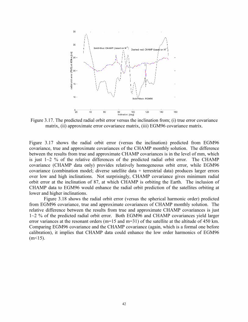
42

Figure 3.17. The predicted radial orbit error versus the inclination from; (i) true error covariance

matrix, (ii) approximate error covariance matrix, (iii) EGM96 covariance matrix. Figure 3.17 shows the radial orbit error (versus the inclination) predicted from EGM96 covariance, true and approximate covariances of the CHAMP monthly solution. The difference between the results from true and approximate CHAMP covariances is in the level of mm, which is just 1~2 % of the relative differences of the predicted radial orbit error. The CHAMP covariance (CHAMP data only) provides relatively homogeneous orbit error, while EGM96 covariance (combination model; diverse satellite data + terrestrial data) produces larger errors over low and high inclinations. Not surprisingly, CHAMP covariance gives minimum radial orbit error at the inclination of 87, at which CHAMP is orbiting the Earth. The inclusion of CHAMP data to EGM96 would enhance the radial orbit prediction of the satellites orbiting at lower and higher inclinations.

Figure 3.18 shows the radial orbit error (versus the spherical harmonic order) predicted from EGM96 covariance, true and approximate covariances of CHAMP monthly solution. The relative difference between the results from true and approximate CHAMP covariances is just 1~2 % of the predicted radial orbit error. Both EGM96 and CHAMP covariances yield larger error variances at the resonant orders (m=15 and m=31) of the satellite at the altitude of 450 km. Comparing EGM96 covariance and the CHAMP covariance (again, which is a formal one before calibration), it implies that CHAMP data could enhance the low order harmonics of EGM96 (m<15).

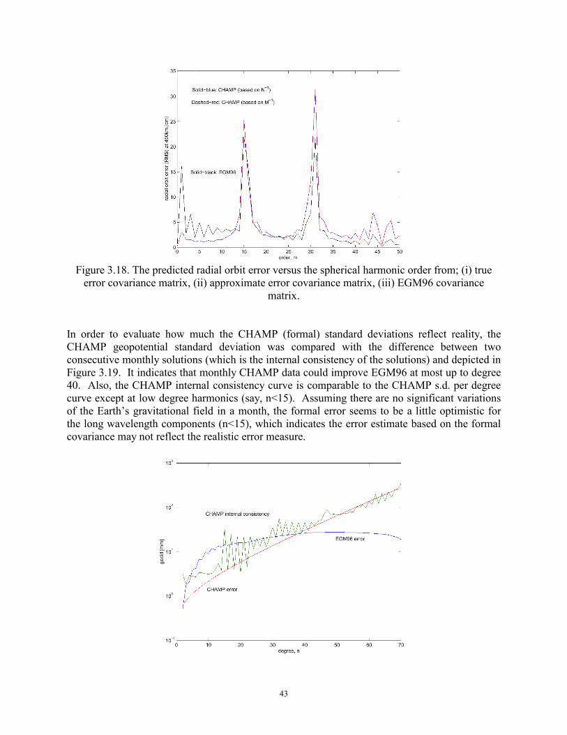
43

Figure 3.18. The predicted radial orbit error versus the spherical harmonic order from; (i) true

error covariance matrix, (ii) approximate error covariance matrix, (iii) EGM96 covariance matrix.

In order to evaluate how much the CHAMP (formal) standard deviations reflect reality, the CHAMP geopotential standard deviation was compared with the difference between two consecutive monthly solutions (which is the internal consistency of the solutions) and depicted in Figure 3.19. It indicates that monthly CHAMP data could improve EGM96 at most up to degree 40. Also, the CHAMP internal consistency curve is comparable to the CHAMP s.d. per degree curve except at low degree harmonics (say, n<15). Assuming there are no significant variations of the Earth’s gravitational field in a month, the formal error seems to be a little optimistic for the long wavelength components (n<15), which indicates the error estimate based on the formal covariance may not reflect the realistic error measure.

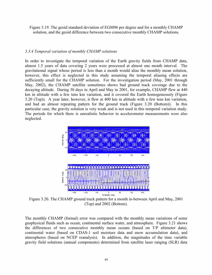
44

Figure 3.19. The geoid standard deviation of EGM96 per degree and for a monthly CHAMP solution, and the geoid difference between two consecutive monthly CHAMP solutions.

3.3.4 Temporal variation of monthly CHAMP solutions In order to investigate the temporal variation of the Earth gravity fields from CHAMP data, almost 1.5 years of data covering 2 years were processed at almost one month interval. The gravitational signal whose period is less than a month would alias the monthly mean solution, however, this effect is neglected in this study assuming the temporal aliasing effects are sufficiently small for the CHAMP solution. For the investigation period (May, 2001 through May, 2002), the CHAMP satellite sometimes shows bad ground track coverage due to the decaying altitude. During 30 days in April and May in 2001, for example, CHAMP flew at 440 km in altitude with a few tens km variation, and it covered the Earth homogeneously (Figure 3.20 (Top)). A year later, however, it flew at 400 km in altitude with a few tens km variation, and had an almost repeating pattern for the ground track (Figure 3.20 (Bottom)). In this particular case, the gravity solution is very weak and is not used in this temporal variation study. The periods for which there is unrealistic behavior in accelerometer measurements were also neglected.

Figure 3.20. The CHAMP ground track pattern for a month in-between April and May, 2001

(Top) and 2002 (Bottom). The monthly CHAMP (formal) error was compared with the monthly mean variations of some geophysical fluids such as ocean, continental surface water, and atmosphere. Figure 3.21 shows the differences of two consecutive monthly mean oceans (based on T/P altimeter data), continental water (based on CDAS-1 soil moisture data and snow accumulation data), and atmospheres (based on NCEP reanalysis). In addition, the magnitudes of the time variable gravity field solutions (annual components) determined from satellite laser ranging (SLR) data

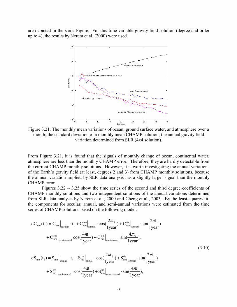
45

are depicted in the same Figure. For this time variable gravity field solution (degree and order up to 4), the results by Nerem et al. (2000) were used.

Figure 3.21. The monthly mean variations of ocean, ground surface water, and atmosphere over a

month; the standard deviation of a monthly mean CHAMP solution; the annual gravity field variation determined from SLR (4x4 solution).

From Figure 3.21, it is found that the signals of monthly change of ocean, continental water, atmosphere are less than the monthly CHAMP error. Therefore, they are hardly detectable from the current CHAMP monthly solutions. However, it is worth investigating the annual variations of the Earth’s gravity field (at least, degrees 2 and 3) from CHAMP monthly solutions, because the annual variation implied by SLR data analysis has a slightly larger signal than the monthly CHAMP error. Figures 3.22 ~ 3.25 show the time series of the second and third degree coefficients of CHAMP monthly solutions and two independent solutions of the annual variations determined from SLR data analysis by Nerem et al., 2000 and Cheng et al., 2003. By the least-squares fit, the components for secular, annual, and semi-annual variations were estimated from the time series of CHAMP solutions based on the following model:

),year1

t4sin(S)

year1t4

cos(S

)year1

t2sin(S)

year1t2

cos(S tS)(tdS

),year1

t4sin(C)

year1t4

cos(C

)year1

t2sin(C)

year1t2

cos(C tC)(tdC

iannual-semi

sinnm

iannual-semi

cosnm

iannual

sinnm

iannual

cosnmisecularnminm

iannual-semi

sinnm

iannual-semi

cosnm

iannual

sinnm

iannual

cosnmisecularnminm

ππ

ππ

ππ

ππ

⋅+⋅+

⋅+⋅+⋅=

++

⋅+⋅+⋅=

&

&

(3.10)

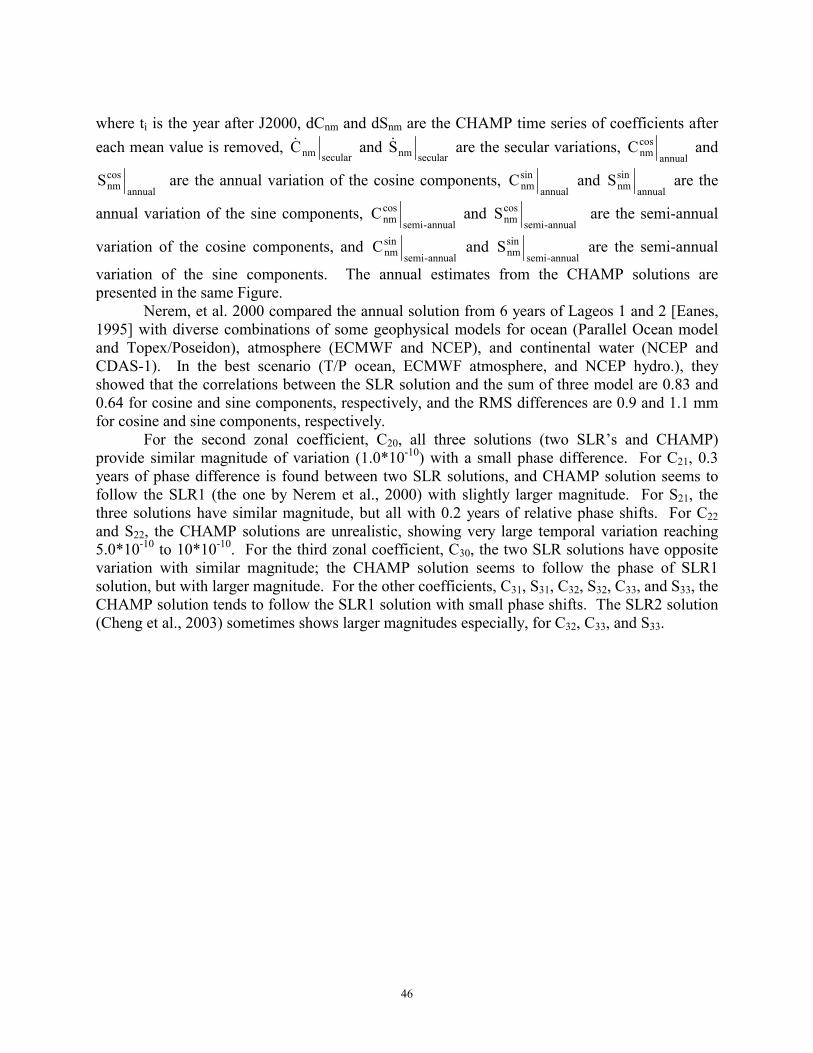
46

where ti is the year after J2000, dCnm and dSnm are the CHAMP time series of coefficients after each mean value is removed,

secularnmC& and secularnmS& are the secular variations,

annualcosnmC and

annualcosnmS are the annual variation of the cosine components,

annualsinnmC and

annualsinnmS are the

annual variation of the sine components, annual-semi

cosnmC and

annual-semicosnmS are the semi-annual

variation of the cosine components, and annual-semi

sinnmC and

annual-semisinnmS are the semi-annual

variation of the sine components. The annual estimates from the CHAMP solutions are presented in the same Figure.

Nerem, et al. 2000 compared the annual solution from 6 years of Lageos 1 and 2 [Eanes, 1995] with diverse combinations of some geophysical models for ocean (Parallel Ocean model and Topex/Poseidon), atmosphere (ECMWF and NCEP), and continental water (NCEP and CDAS-1). In the best scenario (T/P ocean, ECMWF atmosphere, and NCEP hydro.), they showed that the correlations between the SLR solution and the sum of three model are 0.83 and 0.64 for cosine and sine components, respectively, and the RMS differences are 0.9 and 1.1 mm for cosine and sine components, respectively. For the second zonal coefficient, C20, all three solutions (two SLR’s and CHAMP) provide similar magnitude of variation (1.0*10-10) with a small phase difference. For C21, 0.3 years of phase difference is found between two SLR solutions, and CHAMP solution seems to follow the SLR1 (the one by Nerem et al., 2000) with slightly larger magnitude. For S21, the three solutions have similar magnitude, but all with 0.2 years of relative phase shifts. For C22 and S22, the CHAMP solutions are unrealistic, showing very large temporal variation reaching 5.0*10-10 to 10*10-10. For the third zonal coefficient, C30, the two SLR solutions have opposite variation with similar magnitude; the CHAMP solution seems to follow the phase of SLR1 solution, but with larger magnitude. For the other coefficients, C31, S31, C32, S32, C33, and S33, the CHAMP solution tends to follow the SLR1 solution with small phase shifts. The SLR2 solution (Cheng et al., 2003) sometimes shows larger magnitudes especially, for C32, C33, and S33.

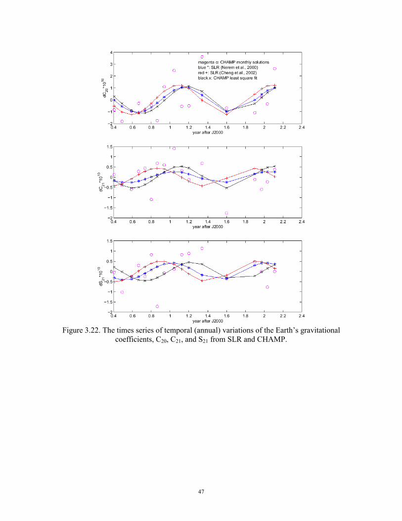
47

Figure 3.22. The times series of temporal (annual) variations of the Earth’s gravitational

coefficients, C20, C21, and S21 from SLR and CHAMP.

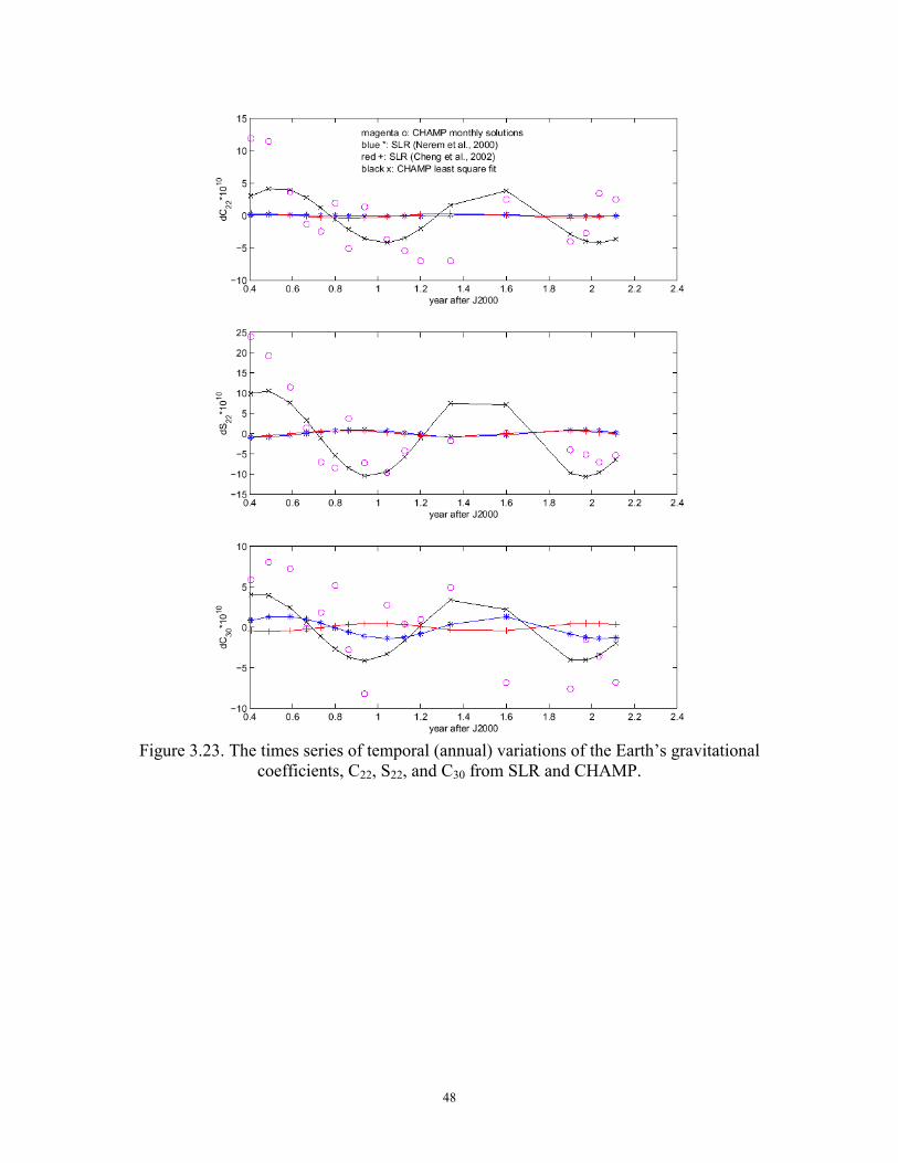
48

Figure 3.23. The times series of temporal (annual) variations of the Earth’s gravitational

coefficients, C22, S22, and C30 from SLR and CHAMP.

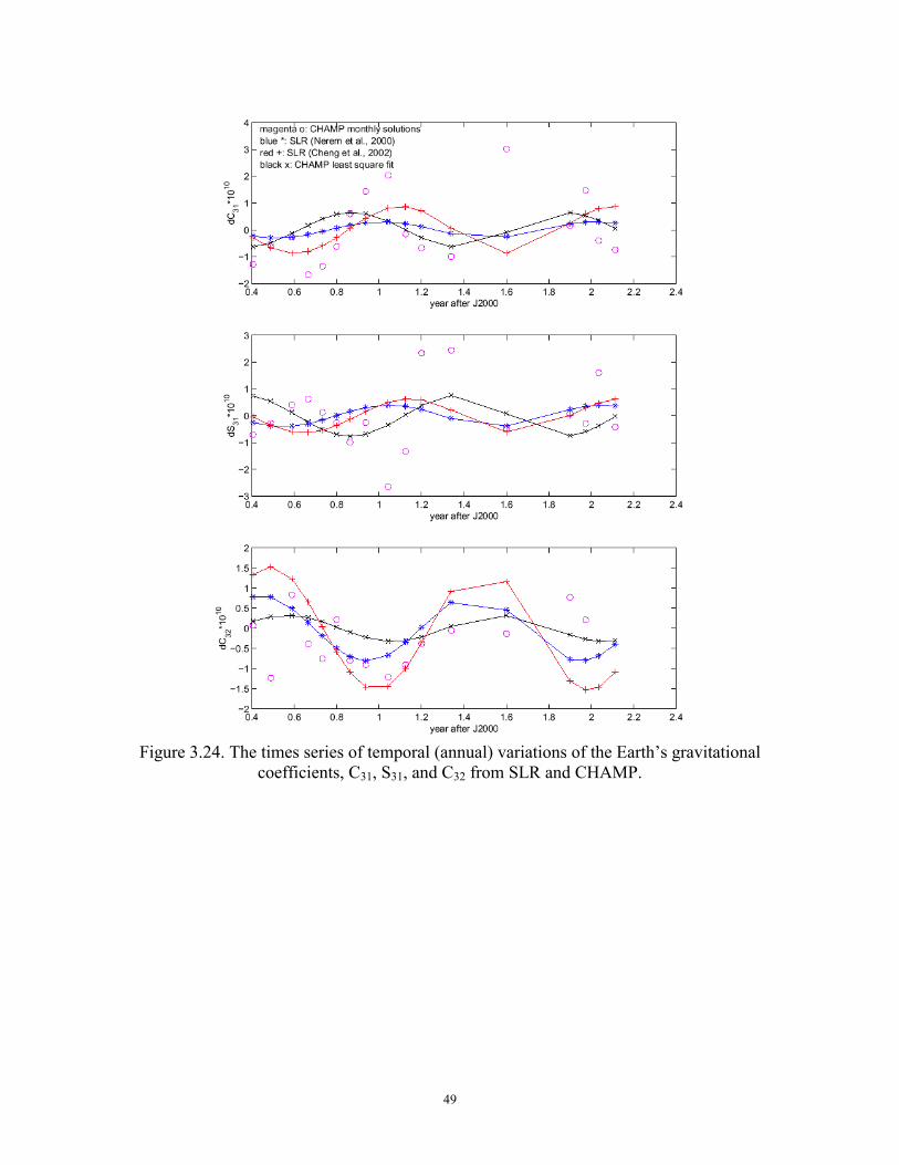
49

Figure 3.24. The times series of temporal (annual) variations of the Earth’s gravitational

coefficients, C31, S31, and C32 from SLR and CHAMP.

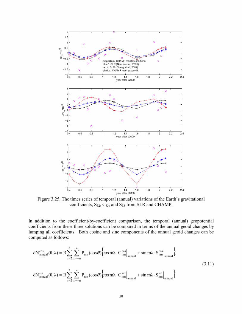
50

Figure 3.25. The times series of temporal (annual) variations of the Earth’s gravitational

coefficients, S32, C33, and S33 from SLR and CHAMP. In addition to the coefficient-by-coefficient comparison, the temporal (annual) geopotential coefficients from these three solutions can be compared in terms of the annual geoid changes by lumping all coefficients. Both cosine and sine components of the annual geoid changes can be computed as follows:

{ }

{ },SmλsinCmλcos)(cosPR)λθ,(dN

,SmλsinCmλcos)(cosPR)λθ,(dN

3

2n

n

nmannual

sinnmannual

sinnmnm

sinannual

3

2n

n

nmannual

cosnmannual

cosnmnm

cosannual

∑ ∑

∑ ∑

= −=

= −=

⋅+⋅=

⋅+⋅=

θ

θ

(3.11)

51

where )λθ,(dNcos

annual and )λθ,(dNsinannual are the annual geoid changes of the cosine and sine

components at co-latitude θ and longitude λ, respectively. However, in this geoid computation, the coefficients, C22, S22, and C30 were excluded, because of CHAMP’s unrealistically large variations compared to SLR. If C22, S22, and C30 are included in the geoid change computation, the consequent unrealistic variation would dominate and make the comparison useless. Figures 3.26 and 3.27 present the cosine and sine components of the three annual geoid changes computed using (11) based on the SLR1, SLR2, and CHAMP solutions. Some statistics for these maps are given in Tables 3.5 ~ 3.7.

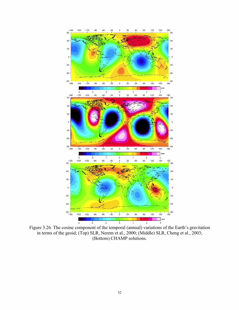
52

Figure 3.26. The cosine component of the temporal (annual) variations of the Earth’s gravitation

in terms of the geoid; (Top) SLR, Nerem et al., 2000; (Middle) SLR, Cheng et al., 2003; (Bottom) CHAMP solutions.

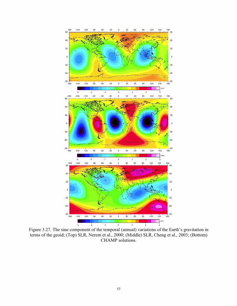
53

Figure 3.27. The sine component of the temporal (annual) variations of the Earth’s gravitation in terms of the geoid; (Top) SLR, Nerem et al., 2000; (Middle) SLR, Cheng et al., 2003; (Bottom)

CHAMP solutions.

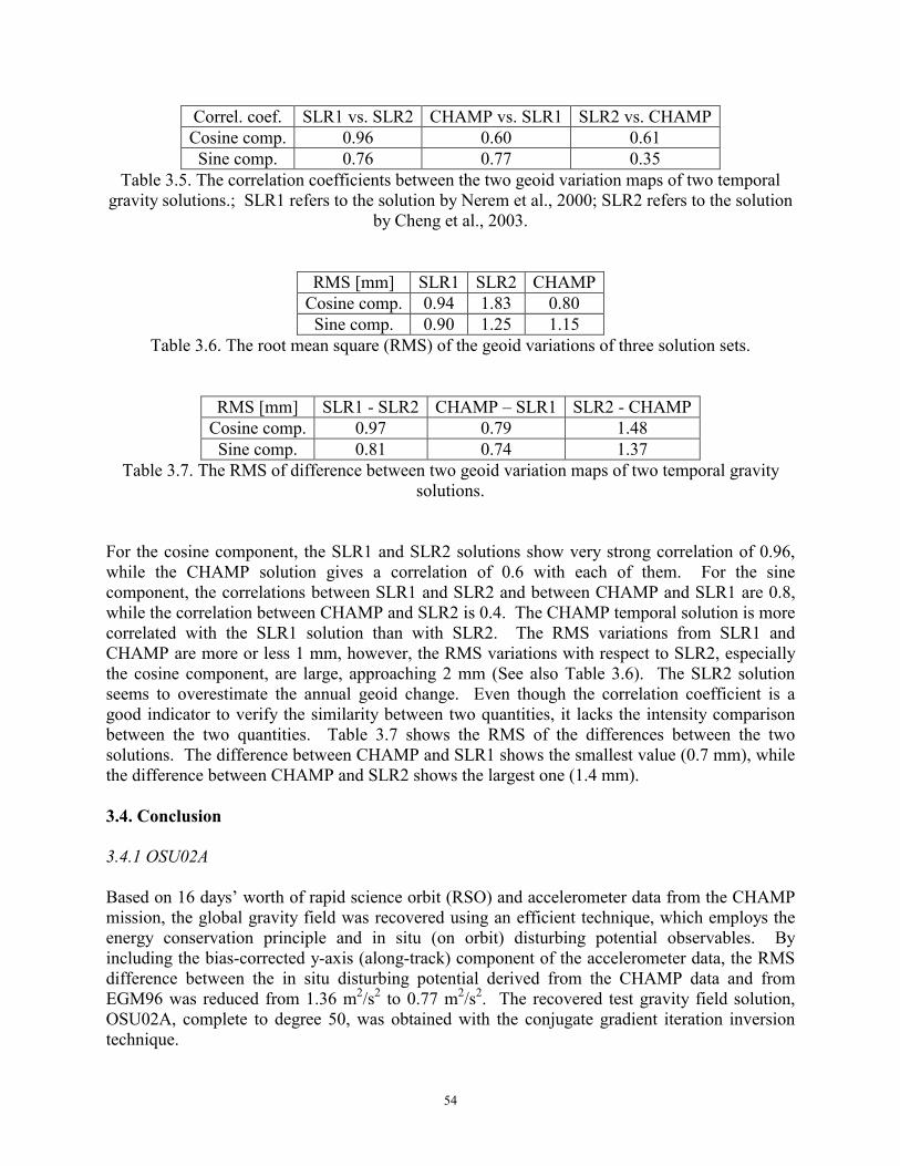
54

Correl. coef. SLR1 vs. SLR2 CHAMP vs. SLR1 SLR2 vs. CHAMP Cosine comp. 0.96 0.60 0.61 Sine comp. 0.76 0.77 0.35

Table 3.5. The correlation coefficients between the two geoid variation maps of two temporal gravity solutions.; SLR1 refers to the solution by Nerem et al., 2000; SLR2 refers to the solution

by Cheng et al., 2003.

RMS [mm] SLR1 SLR2 CHAMPCosine comp. 0.94 1.83 0.80 Sine comp. 0.90 1.25 1.15

Table 3.6. The root mean square (RMS) of the geoid variations of three solution sets.

RMS [mm] SLR1 - SLR2 CHAMP – SLR1 SLR2 - CHAMP Cosine comp. 0.97 0.79 1.48 Sine comp. 0.81 0.74 1.37

Table 3.7. The RMS of difference between two geoid variation maps of two temporal gravity solutions.

For the cosine component, the SLR1 and SLR2 solutions show very strong correlation of 0.96, while the CHAMP solution gives a correlation of 0.6 with each of them. For the sine component, the correlations between SLR1 and SLR2 and between CHAMP and SLR1 are 0.8, while the correlation between CHAMP and SLR2 is 0.4. The CHAMP temporal solution is more correlated with the SLR1 solution than with SLR2. The RMS variations from SLR1 and CHAMP are more or less 1 mm, however, the RMS variations with respect to SLR2, especially the cosine component, are large, approaching 2 mm (See also Table 3.6). The SLR2 solution seems to overestimate the annual geoid change. Even though the correlation coefficient is a good indicator to verify the similarity between two quantities, it lacks the intensity comparison between the two quantities. Table 3.7 shows the RMS of the differences between the two solutions. The difference between CHAMP and SLR1 shows the smallest value (0.7 mm), while the difference between CHAMP and SLR2 shows the largest one (1.4 mm). 3.4. Conclusion 3.4.1 OSU02A Based on 16 days’ worth of rapid science orbit (RSO) and accelerometer data from the CHAMP mission, the global gravity field was recovered using an efficient technique, which employs the energy conservation principle and in situ (on orbit) disturbing potential observables. By including the bias-corrected y-axis (along-track) component of the accelerometer data, the RMS difference between the in situ disturbing potential derived from the CHAMP data and from EGM96 was reduced from 1.36 m2/s2 to 0.77 m2/s2. The recovered test gravity field solution, OSU02A, complete to degree 50, was obtained with the conjugate gradient iteration inversion technique.

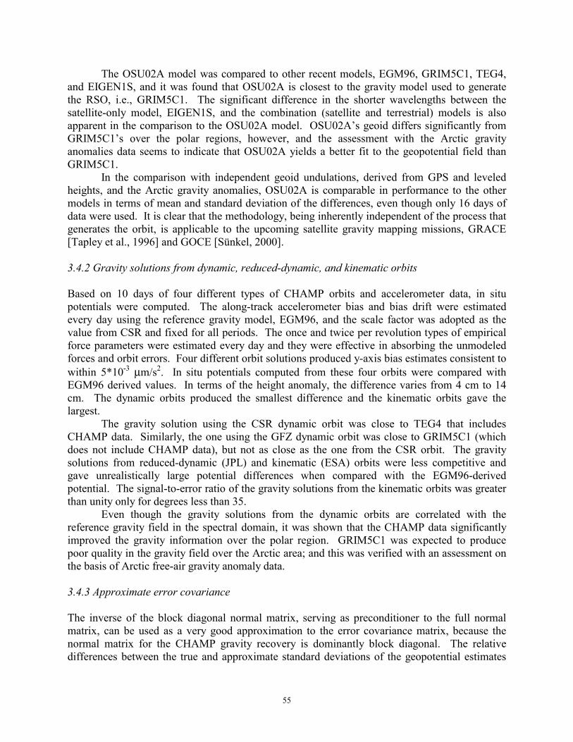
55

The OSU02A model was compared to other recent models, EGM96, GRIM5C1, TEG4, and EIGEN1S, and it was found that OSU02A is closest to the gravity model used to generate the RSO, i.e., GRIM5C1. The significant difference in the shorter wavelengths between the satellite-only model, EIGEN1S, and the combination (satellite and terrestrial) models is also apparent in the comparison to the OSU02A model. OSU02A’s geoid differs significantly from GRIM5C1’s over the polar regions, however, and the assessment with the Arctic gravity anomalies data seems to indicate that OSU02A yields a better fit to the geopotential field than GRIM5C1. In the comparison with independent geoid undulations, derived from GPS and leveled heights, and the Arctic gravity anomalies, OSU02A is comparable in performance to the other models in terms of mean and standard deviation of the differences, even though only 16 days of data were used. It is clear that the methodology, being inherently independent of the process that generates the orbit, is applicable to the upcoming satellite gravity mapping missions, GRACE [Tapley et al., 1996] and GOCE [Sünkel, 2000]. 3.4.2 Gravity solutions from dynamic, reduced-dynamic, and kinematic orbits Based on 10 days of four different types of CHAMP orbits and accelerometer data, in situ potentials were computed. The along-track accelerometer bias and bias drift were estimated every day using the reference gravity model, EGM96, and the scale factor was adopted as the value from CSR and fixed for all periods. The once and twice per revolution types of empirical force parameters were estimated every day and they were effective in absorbing the unmodeled forces and orbit errors. Four different orbit solutions produced y-axis bias estimates consistent to within 5*10-3 µm/s2. In situ potentials computed from these four orbits were compared with EGM96 derived values. In terms of the height anomaly, the difference varies from 4 cm to 14 cm. The dynamic orbits produced the smallest difference and the kinematic orbits gave the largest. The gravity solution using the CSR dynamic orbit was close to TEG4 that includes CHAMP data. Similarly, the one using the GFZ dynamic orbit was close to GRIM5C1 (which does not include CHAMP data), but not as close as the one from the CSR orbit. The gravity solutions from reduced-dynamic (JPL) and kinematic (ESA) orbits were less competitive and gave unrealistically large potential differences when compared with the EGM96-derived potential. The signal-to-error ratio of the gravity solutions from the kinematic orbits was greater than unity only for degrees less than 35. Even though the gravity solutions from the dynamic orbits are correlated with the reference gravity field in the spectral domain, it was shown that the CHAMP data significantly improved the gravity information over the polar region. GRIM5C1 was expected to produce poor quality in the gravity field over the Arctic area; and this was verified with an assessment on the basis of Arctic free-air gravity anomaly data. 3.4.3 Approximate error covariance The inverse of the block diagonal normal matrix, serving as preconditioner to the full normal matrix, can be used as a very good approximation to the error covariance matrix, because the normal matrix for the CHAMP gravity recovery is dominantly block diagonal. The relative differences between the true and approximate standard deviations of the geopotential estimates

56

are less than 1 %. From the error covariance propagation tests for the geoid and gravity anomaly, and the radial orbit accuracy, the approximate error covariance provides very similar results to the true error covariance within 1~2 % of relative difference of the predicted accuracy. In addition, it was found that the error propagation based on variances only would fail to provide the predicted accuracy of the geoid and gravity anomaly. Clearly, the results demonstrate that the iterative inversion based on the conjugate gradient with a preconditioner does provide not only the exact estimates but also very accurate least-squares error variance-covariance estimates for the CHAMP global gravity field recovery. By comparing the (formal) standard deviation with the internal consistency of the solutions, it is shown that the CHAMP error variance-covariance may underestimate the actual error level of the low degree coefficient estimates. 3.4.4 Temporal (annual) variation of the Earth gravity field 1.5 years of CHAMP data were processed to investigate some possible temporal variations of the gravitational field. Even though the time span of data covers almost 2 years, some months of data were disregarded, because the CHAMP ground tracks during these periods do not cover the globe entirely and sometimes the accelerometer data are not valid. The time series of CHAMP geopotential estimates of the second and third degrees were modeled with secular, annual, and semi-annual parameters. The annual estimates through a least-squares fit were compared with the currently available annual solution sets from SLR. Although the C22, S22, and C30 estimates show too large variations, other estimates follow SLR solutions quite well. The temporal geoid change maps from the time series of CHAMP solutions (excluding the above three coefficients) have correlations of 0.6 and 0.8 and RMS differences of 0.8 and 0.7 mm for cosine and sine components, respectively, when compared with the SLR solution (Nerem et al., 2000), that was verified with some geophysical models. Interestingly, the CHAMP temporal solution compares better to Nerem et al.’s (2000) solution than does the latter compare to the SLR solution by (Cheng et al., 2003). However, the reason for large variations appearing in the C22, S22, and C30 estimates is not known yet. The semi-annual estimates are not checked, because there is no verified solution for this component. At present, the temporal (annual) gravity solutions have been determined solely from SLR analyses. Even though the results should be investigated by analyzing more data for a longer time span, this result is potentially the first temporal gravity solution from the CHAMP satellite.

57

4. THE EFFICIENT DETERMINATION OF GLOBAL GRAVITY FIELD FROM SATELLITE-TO-SATELLITE TRACKING MISSION, GRACE

4.1. Introduction Since its launch in July 2000, CHAMP [Reigber et al., 1996] gravity and magnetic mapping satellite mission has been providing invaluable data for gravity field studies. During this decade, measurements from the gravity mapping missions, GRACE [Tapley et al., 1996] and GOCE [Rummel et al., 1999], are expected to provide significant improvement in our knowledge of the Earth's mean gravity field and its temporal variation. It is expected that the mean geoid would be improved to one cm accuracy at a wavelength of 100 km or longer (primarily by GOCE), and the time-varying mass variations of the Earth system in terms of climate-sensitive signals could be measured with sub-centimeter accuracy in units of column of water movement near the Earth’s surface with a spatial resolution of 250 km or longer, and a temporal resolution of weeks (primarily by GRACE). Gravity Recovery and Climate Experiment (GRACE) was launched on March 17, 2002 for a mission span of 5 years or longer. The mission consists of two identical co-orbiting spacecraft with a separation of 220±50 km at a mean initial orbital altitude of 485 km, with a circular orbit, and an inclination of 89° for near-global coverage [Thomas, 1999; GRACE Science Mission Requirement Document, 2000; Bettadpur and Watkins, 2000]. The scientific objectives of GRACE include the mapping and understanding of climate-change signals associated with mass variations within the solid Earth – atmosphere – ocean – cryosphere - hydrosphere system and with unprecedented accuracy and resolution in the form of the time-varying gravity field [e.g., Wahr et al., 1998]. In addition to a new model of the Earth’s static gravity field, time-varying fields will be available every 30 days for a time span of 5 years. The dual one-way K- (24.5 GHz) and Ka- (32.7 GHz) band microwave inter-satellite ranging system with a precision of 10 µm [Kim et al., 2001], the Ultra-Stable Oscillator (USO) accurate to within 70 picoseconds for time-tagging, the 3-axis super-STAR accelerometers with a precision of 4x10-12 m/s2 [Davis et al., 1999; Perret et al., 2001], and the dual-frequency 24-channel Blackjack GPS receivers comprise GRACE’s instrument suite.

One way to analyze low-low SST and accelerometry data is to apply the traditional method whereby the geopotential coefficients are estimated from tracking data by numerically integrating the satellite’s equations of motion and variationals (See also Rowlands et al.(2002) who estimate the geopotential from short arcs of tracking data). In this study, we develop an alternative (and more straightforward) algorithm to estimate the Earth’s gravitational harmonic coefficients based on a linear boundary value problem in the potential theory [Heiskanen and Moritz, 1967]. The potential difference values between the two satellites along the orbit can be computed by combining the inter-satellite range rate, position, velocity, and acceleration data through the energy conservation principle [Jekeli, 1999]. The computed potential differences are treated as boundary values on a fixed boundary, i.e., the orbit. Using the energy conservation principle has been successfully demonstrated recently by analyzing actual CHAMP data [Han et al., 2002a; Gerlach et al., 2002; Sneeuw et al., 2002]. Here, we extend this approach in a very efficient manner to the recovery of GRACE static as well as temporal gravity fields complete up to degree and order 120.

The end-to-end algorithm with the in situ potential difference observations is formulated using spherical harmonic functions as representational basis in a space-wise approach [Klees et

58

al., 2000a]. In this approach, the observations would be reduced or interpolated onto a regular grid that yields a tractable normal matrix, e.g., with block-diagonal structure. That is, the boundary values should be distributed regularly in longitude (but not necessarily in the latitude), the geometric radii should be independent of longitude, and an error covariance matrix should be diagonal with variances independent of longitude [Colombo, 1981, Jekeli, 1996]. In this study, however, we solve the boundary value problem in the space-wise approach without any data reduction or interpolation. That is, the measurements are used at their exact observation locations. The irregularly distributed data produce a fully populated normal matrix, which involves massive computations. To avoid the explicit computation of the normal matrix, the conjugate gradient method is applied to compute geopotential coefficients from monthly GRACE data. An appropriate pre-conditioner like a block-diagonal matrix (which contains most of power of the full normal matrix) is used to accelerate the convergence rate. This efficient solution method has been suggested to produce a very high degree geopotential field (Nmax=200 or more) from the future European gravity gradiometer mission, GOCE [Schuh, 1996; Schuh et al., 1996; Klees et al., 2001b; Ditmar and Klees, 2002]. Even though this method provides the exact solution very efficiently, it does not produce a complete error covariance matrix of the estimated geopotential coefficients, which constitutes a significant drawback. In this study, however, we will present not only the exact estimates of the solutions but also a very good approximation of the error variance-covariance matrix obtained without additional computations. We will quantify the quality of the approximate covariance matrix, as well. Based on the developed method, results on the static and temporal gravity field recovery including the continental water mass redistribution are presented. The previous simulation studies, e.g., by Wahr et al.(1998) and Nerem et al.(2002), computed the spherical harmonic coefficients for ocean and continental surface water mass and added random noises to the coefficients according to the GRACE error degree variance model. The applied random errors had different variances only along the spherical harmonic degrees, and they are independently and uniformly distributed along the spherical harmonic orders. Then, they performed spatial averaging in the spectral domain to reduce higher degree and order errors, obtaining an accurate long wavelength signal of temporal gravity. It is a limited analysis in the spectral domain and no inversion of GRACE data was involved in this approach as noted by Wahr and Velicogna (2002). Here, we add the temporal gravity signals to the GRACE measurements for a month and estimate the spherical harmonic coefficients complete up to degree and order 120 in the presence of both measurement noise and temporal gravity signals. Therefore, we are able to investigate the feasibility to recover the time-variable gravity field under the influence of measurement noise as well as temporal aliasing of the signals. 4.2. In situ observables 4.2.1 Satellite-to-satellite tracking measurements The GRACE mission provides very precise range measurements between two satellites tracking each other along approximately the same orbit. Using the position vectors of the two satellites, x1 and x2, the inter-satellite range, ρ12, can be expressed as follows:

( ) ( ) ,ρ 1212121212 exxxxx ⋅=−⋅−= (4.1)

59

where x12 = x2 − x1 and e12 is the line-of-sight (LOS) unit vector, pointing to the second satellite from the first satellite. In order to obtain high precision measurements, both GRACE satellites transmit and receive dual frequency microwaves in the K (24.5GHz) and Ka (32.7GHz) bands. Two frequencies are used to reduce significantly the first order frequency-dependent ionospheric delays. By differentiating the range measurements, the range rate is obtained as follows:

.ρ 121212 ex ⋅= && (4.2) The post-processed range-rate data from GRACE represent an integration time of 5 seconds and have an expected accuracy of 0.1 µm/s (RMS) [Kim et al., 1999]. This type of along-track measurement is very sensitive to the geophysical fluid mass redistribution under the orbits and it is a fundamental quantity used to solve for the Earth’s global (static and temporal) gravity field. 4.2.2 In situ potential observable In Chapter 2 and Chapter 3, an accurate model was derived and studied relating the Earth’s gravitational potential, VE, to x, x& , and F in the inertial frame, where x is the position vector, x& is the velocity vector, and F designates the net force vector including all non-conservative forces measured by the accelerometer:

( ) 0Tii

1i2

i2

i1e

2iE VVdtxxxxω

21V −−⋅−−−≈ ∫ xFx &&&& , (4.3)

where Ti

3i2

i1

i ][ xxx=x and Ti3

i2

i1

i ][ xxx &&&& =x , and superscript, i, denotes inertial frame. The harmonic geopotential coefficients can be estimated from a global distribution of observations of VE. The first term in (4.3) is the kinetic energy (per unit mass) of the satellite, determined by its inertial velocity. The second term is the so-called ‘potential rotation’ term that accounts for the (dominant) rotation of Earth’s potential in the inertial frame. The third term is the dissipating energy due to the atmospheric drag, solar radiation pressure, thermal forces, and other non-conservative forces. The term, VT, stands for the temporal variation of the gravitational potential including N-body effects, ocean tides, atmosphere, ground water, and so on. The last term is the energy constant of the system including a constant zero-degree harmonic of the gravitational potentials. This type of observation may be obtained from CHAMP, the GRACE satellites, and any other GPS-tracked Earth orbiting satellite, as long as F can be determined accurately. Analysis based on actual CHAMP-GPS data indicates that this in situ observation model produces promising results [Gerlach et al., 2002; Han et al., 2002a; Sneeuw et al., 2002; Visser et al., 2002]. 4.2.3 In situ potential difference observable The in situ observable of interest is the potential difference between two satellites expected only from the low-low satellite-to-satellite tracking mission, GRACE. It can be computed from range-rates, velocity vectors, and position vectors in the inertial frame. The following approximate model was developed and used by Wolff (1969), Rummel (1980), and Jekeli and Rapp (1980):

60

12i11212 ρVVV &&x≈−= . (4.4)

This model, relating the in situ inter-satellite range rate measurements to the gravitational potential difference between two satellites, V12, is not appropriate to take full advantage of the current instrument’s capability. Specifically, it does not include the time-variable effect on the gravitational potential due to Earth’s rotation, which is significant on the order of ±1 m2/s2. A more rigorous model was developed by Jekeli (1999) via the energy conservation principle. Correcting the mistakes in (27) of Jekeli (1999), reformulating it in terms of the disturbing potential (Earth’s gravitational potential minus normal gravitational potential) difference, T12, instead of the residual potential difference, and assuming the energy dissipation term is obtained from measuring non-gravitational accelerations, the correct formula is given by:

( ) 0T1122124321120112 δVδVdtδVRvvvvρδT −−⋅−⋅−+++++= ∫ xFxFx &&&& , (4.5)

where

( ) 121201

021v xδexx &&& ⋅−= ,

( ) 01212

0112v xδexxδ ⋅−= && ,

1213v xδxδ && ⋅= , 2

124 21v xδ&= , and

( ) ( ) ( ) ( ){ }101

02

02

012

01

02

02

011122121221e12 xxxxxxxxxxxxxxxxωδVR &&&&&&&& −+−−−−−= .

For the simplicity of the notations, the superscript, i, denoting inertial frame was dropped. The superscript, 0, denotes a quantity based on the known reference field, and the symbol, δ, indicates a residual quantity between the true field and the reference field. The sixth term of the right hand side is the potential rotation difference between two satellites, which can be computed with a linear combination of positions and velocities of two satellites in both fields. The seventh term is the dissipating energy difference between the two satellites. The on-board accelerometer measurements to capture all non-conservative forces acting on the satellites (after calibration) can be used to compute this term. The eighth and last terms are the residual temporal variation of gravitational potential and the residual energy constant of the system, respectively. This model indicates that the accurate potential difference between two satellites can be obtained by measuring the inter-satellite range rate as well as the position vectors and velocity vectors, which are available from GPS and high precision range measurements.

The expected range-rate accuracy from K-band ranging of GRACE mission of about 0.1 µm/s corresponds to a potential difference accuracy of about 10-3 m2/s2. In order to take full advantage of this high-precision in the range-rate measurements, the commensurate error of a single satellite’s position and velocity should be better than 7 cm and 5 µm/s, respectively, and that of the inter-satellite baseline position and velocity should be better than 0.1 mm and 2 µm/s, respectively, [Jekeli, 1999]. These high precision orbital parameters might be obtainable with the aid of high precision range and rage-rate measurements together with the Blackjack-class

61

GPS receiver. The registration or coordinatization of the observable causes error as well, because of the imperfect orbit. However, the GRACE potential difference observable is not very sensitive to this error, because the orbit errors of the two satellites would be highly correlated [Jekeli and Garcia, 2001]. The orbit, therefore, is fixed when the relationship between the observable and the unknown geopotential coefficients is established in the following section. 4.3. Observation model and characteristics of the normal matrix 4.3.1 Linear observation model for potential difference The in situ observable, i.e., the disturbing potential difference between the two satellites, can be decomposed into a series of spherical harmonic functions. By fixing the satellite orbits, the linear relationship between the observations and the unknown geopotential coefficients is obtained as follows:

∑∑∞

= =++

++

−

+

−

=

−=

2n

n

0m

nm22nm

1n

211nm

1n

1

nm22nm

1n

211nm

1n

1

222,2111,1222,111,12

Smλsin)θ(cosPrRmλsin)θ(cosP

rR

Cmλcos)θ(cosPrRmλcos)θ(cosP

rR

RGM

)λ,θ(rT )λ,θ(rT)λ,θr,λ,θ(rT

, (4.6)

where GM is the gravitational constant times the mass of the Earth, R is the Earth’s mean radius, (r1,θ1,λ1) and (r2,θ2,λ2) are the coordinates of the 1st and 2nd satellite, respectively, nmP is the fully-normalized, associated Legendre function of degree n and order m, nmC and nmS are the unknown spherical harmonic coefficients of degree n and order m.

Interchanging the sequence of the two summations and truncating the infinite series expansion to a finite degree, the following equation is obtained:

∑ ∑= =

++

++

−

+

−

=Nmax

0m

Nmax

mn

nm222,snm

1n

2111,

snm

1n

1

nm222,cnm

1n

2111,

cnm

1n

1

0

222,111,12

S)λ,θr(YrR)λ,θr(Y

rR

C)λ,θr(YrR)λ,θr(Y

rR

U

)λ,θr,λ,θ(rT

, (4.7)

whereR

GMU0 = ,

iinmiiicnm mλcos)θ(cosP)λ,θ,(rY = ,

iinmiiisnm mλsin)θ(cosP)λ,θ,(rY = , i=1 or 2.

62

The observation, T12, is obtained along the satellites’ orbit and is sampled regularly in time. Now, the problem is to estimate optimally the geopotential coefficients from T12 observations based on the given linear relationship. Let y be the vector of observations and let e be the corresponding observation error vector. The parameter vector, x, contains the geopotential coefficients up to a certain maximum degree and order, Nmax. Using the weight matrix (inverse of cofactor matrix), P, the linear observation equations can be expressed by

)σ,(~ , 12 −⋅=+ P0exAey , (4.8) The parameter vector is ordered as follows:

TmaxN10 ][ xxxx L= , (4.9) where T

mNmax,m1,mmm,mNmax,m1,mmm,m ]SSSCCC[ LL ++=x and the superscript,

T, denotes the transpose of the column vector. The design matrix, A, is computed based on the exact observation equations given in (4.7). If the i-th component in the observation vector is denoted as )λ,θ,r,λ,θ,(rT i

2i2

i2

i1

i1

i1

i12 and the i-th row vector of the design matrix, A, is expressed

by )λ,θ,r,λ,θ,(r i2

i2

i2

i1

i1

i1

Tia , then the i-th observable is represented by the multiplication of two

vectors, i.e., xaTi

i12T = . The three errors associated with this representation are i) error in the

observable, i12T , ii) spherical harmonics truncation error (or modeling error) in both of T

ia and x , iii) error in the vector, T

ia , which is the registration error, basically due to the orbit error. Except for the measurement error in i

12T , the other errors are disregarded in this study. Once the linear observation equation is established as in (4.8), and the weight matrix is assumed to be the identity matrix (which is the case for independently and identically distributed noise), the least-squares solution is obtained as follows:

AANyAxN TT where,ˆ == . (4.10) In order to compute the normal matrix, N, and the vector, ATy, we need to calculate the sum of dyadic products of all row vectors in the design matrix and the sum of products of each row vector with an observation vector component, respectively. That is,

∑∑==

==Nobs

1iii

TNobs

1i

Tii y , ayAaaN , (4.11)

where Nobs is the number of observations. The normal matrix, N, computed from the exact design matrix implied by (4.7), is a fully populated matrix, because the potential difference observations refer to the actual satellite positions, which form an irregular boundary. Usually, it is a very large full matrix whose size is (Nmax+1)2 by (Nmax+1)2. In addition, it can be shown that the normal matrix has a block-diagonally dominant form once the unknown coefficients are

63

ordered as in (4.9). This characteristic can be used to accelerate the convergence of the iterative solution as we discuss in the next section. 4.3.2 Block-diagonally dominant normal matrix In order to check the block-diagonally dominant characteristic of the normal matrix, assume that the two radii of the satellites are the same as r; then the following approximate form is obtained:

{ }{ }∑ ∑

= =

+

+

+−

=

Nmax

0m

Nmax

mn nm21nm21nm

nm21nm21nm1n

0

221112

Smλcos)θ,θ(ηmλsin)θ,θ(χCmλsin)θ,θ(ηmλcos)θ,θ(χ

rRU

)λ,θ,λ,θ(r,T

, (4.12)

where

θ22nmθ11nm21nm mλcos)θ(cosPmλcos)θ(cosP)θ,θ(χ −= ,

θ22nmθ11nm21nm mλsin)θ(cosPmλsin)θ(cosP)θ,θ(η −= , λ1=λθ1+λ, λ2=λθ2+λ, λθ1 and λθ2 are called the longitude corrections for the first and the second satellites, respectively, λ is called the reference longitude. Consider an ascending orbital arc to see how the reference longitude and the longitude corrections are determined. As Figure 4.1 shows, the reference longitude of each orbital arc is the longitude where the arc crosses the equator. The longitude correction is the departure of the satellite’s longitude from the reference longitude. Its magnitude depends on the latitude and the inclination of the orbit, and its sign depends on the latitude and direction of the orbit, i.e., ascending or descending. The longitude correction values can be represented approximately as a function of the latitude only for every ascending or descending arc. With this approximation, λθ1, λθ2, )θ,θ(χ 21nm , and )θ,θ(η 21nm depend only on the latitudes, 1θ and 2θ . Therefore, we can interpret equation (4.12) as expressing T12 in terms of only one longitude, the reference longitude.

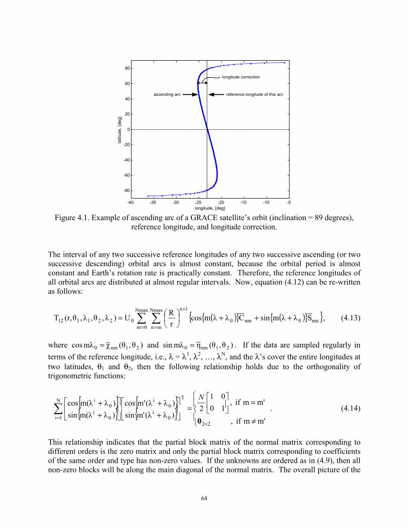
64

-40 -35 -30 -25 -20 -15 -10 -5

-80

-60

-40

-20

0

20

40

60

80

longitude, [deg]

latit

ude,

[deg

]

reference longitude of this arcascending arc

longitude correction

Figure 4.1. Example of ascending arc of a GRACE satellite’s orbit (inclination = 89 degrees),

reference longitude, and longitude correction. The interval of any two successive reference longitudes of any two successive ascending (or two successive descending) orbital arcs is almost constant, because the orbital period is almost constant and Earth’s rotation rate is practically constant. Therefore, the reference longitudes of all orbital arcs are distributed at almost regular intervals. Now, equation (4.12) can be re-written as follows:

( ){ } ( ){ }{ }∑ ∑= =

+

+++

=

Nmax

0m

Nmax

mnnm0nm0

1n

0221112 SλλmsinCλλmcosrRU)λ,θ,λ,θ(r,T , (4.13)

where )θ,θ(χmλcos 21nm0 = and )θ,θ(ηmλsin 21nm0 = . If the data are sampled regularly in terms of the reference longitude, i.e., λ = λ1, λ2, …, λN, and the λ’s cover the entire longitudes at two latitudes, θ1 and θ2, then the following relationship holds due to the orthogonality of trigonometric functions:

{ }{ }

{ }{ }

≠

=

=

++

++

×=∑

m' m if ,

m'm if , 1001

2)λ(λm'sin)λ(λm'cos

)λm(λsin)λm(λcos

22

T

0i

0iN

1i 0i

0i

0

N. (4.14)

This relationship indicates that the partial block matrix of the normal matrix corresponding to different orders is the zero matrix and only the partial block matrix corresponding to coefficients of the same order and type has non-zero values. If the unknowns are ordered as in (4.9), then all non-zero blocks will be along the main diagonal of the normal matrix. The overall picture of the

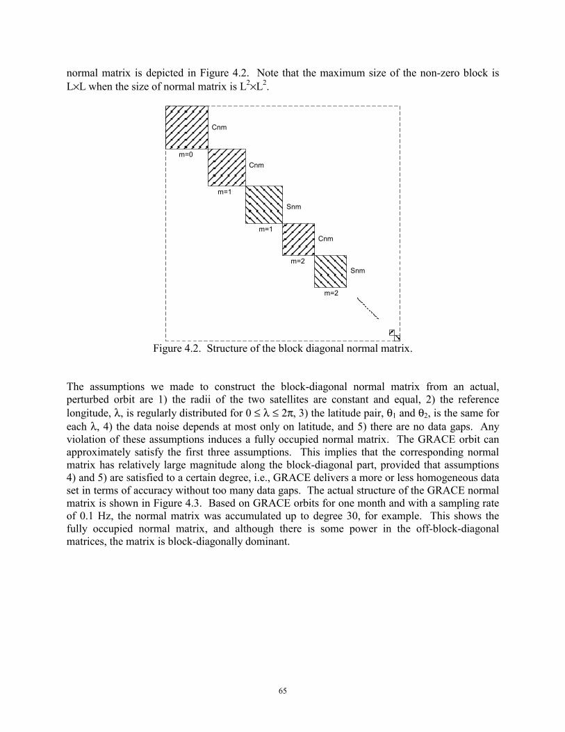
65

normal matrix is depicted in Figure 4.2. Note that the maximum size of the non-zero block is L×L when the size of normal matrix is L2×L2.

m=0

m=1

m=1

Cnm

Cnm

m=2

m=2

Cnm

Snm

Snm

Figure 4.2. Structure of the block diagonal normal matrix.

The assumptions we made to construct the block-diagonal normal matrix from an actual, perturbed orbit are 1) the radii of the two satellites are constant and equal, 2) the reference longitude, λ, is regularly distributed for 0 ≤ λ ≤ 2π, 3) the latitude pair, θ1 and θ2, is the same for each λ, 4) the data noise depends at most only on latitude, and 5) there are no data gaps. Any violation of these assumptions induces a fully occupied normal matrix. The GRACE orbit can approximately satisfy the first three assumptions. This implies that the corresponding normal matrix has relatively large magnitude along the block-diagonal part, provided that assumptions 4) and 5) are satisfied to a certain degree, i.e., GRACE delivers a more or less homogeneous data set in terms of accuracy without too many data gaps. The actual structure of the GRACE normal matrix is shown in Figure 4.3. Based on GRACE orbits for one month and with a sampling rate of 0.1 Hz, the normal matrix was accumulated up to degree 30, for example. This shows the fully occupied normal matrix, and although there is some power in the off-block-diagonal matrices, the matrix is block-diagonally dominant.

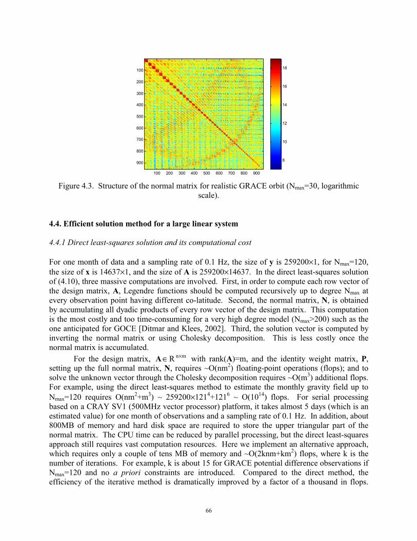
66

100 200 300 400 500 600 700 800 900

100

200

300

400

500

600

700

800

900 8

10

12

14

16

18

Figure 4.3. Structure of the normal matrix for realistic GRACE orbit (Nmax=30, logarithmic

scale). 4.4. Efficient solution method for a large linear system 4.4.1 Direct least-squares solution and its computational cost For one month of data and a sampling rate of 0.1 Hz, the size of y is 259200×1, for Nmax=120, the size of x is 14637×1, and the size of A is 259200×14637. In the direct least-squares solution of (4.10), three massive computations are involved. First, in order to compute each row vector of the design matrix, A, Legendre functions should be computed recursively up to degree Nmax at every observation point having different co-latitude. Second, the normal matrix, N, is obtained by accumulating all dyadic products of every row vector of the design matrix. This computation is the most costly and too time-consuming for a very high degree model (Nmax>200) such as the one anticipated for GOCE [Ditmar and Klees, 2002]. Third, the solution vector is computed by inverting the normal matrix or using Cholesky decomposition. This is less costly once the normal matrix is accumulated.

For the design matrix, mnR ×∈A with rank(A)=m, and the identity weight matrix, P, setting up the full normal matrix, N, requires ~O(nm2) floating-point operations (flops); and to solve the unknown vector through the Cholesky decomposition requires ~O(m3) additional flops. For example, using the direct least-squares method to estimate the monthly gravity field up to Nmax=120 requires O(nm2+m3) ~ 259200×1214+1216 ~ O(1014) flops. For serial processing based on a CRAY SV1 (500MHz vector processor) platform, it takes almost 5 days (which is an estimated value) for one month of observations and a sampling rate of 0.1 Hz. In addition, about 800MB of memory and hard disk space are required to store the upper triangular part of the normal matrix. The CPU time can be reduced by parallel processing, but the direct least-squares approach still requires vast computation resources. Here we implement an alternative approach, which requires only a couple of tens MB of memory and ~O(2knm+km2) flops, where k is the number of iterations. For example, k is about 15 for GRACE potential difference observations if Nmax=120 and no a priori constraints are introduced. Compared to the direct method, the efficiency of the iterative method is dramatically improved by a factor of a thousand in flops.

67

This efficient method was first proposed and successfully demonstrated for GOCE satellite gradiometry [Schuh, 1996, Schuh et al., 1996, Ditmar and Klees, 2002, Pail and Plank, 2002]. 4.4.2 Conjugate gradient with a preconditioner The conjugate gradient method was already discussed in Chapter 2. In this Chapter, it is summarized for the particular application at hand. This method always converges if the normal matrix is positive definite or full rank [Golub and van Loan, 1996]. The essential idea of this method is as follows. An iterate (vector) is updated by adding the increment (vector) to the previous iterate. The direction of the increment vector (or updating vector) is determined as the optimal direction toward the minimum error, which is the gradient direction of squared error norm with an appropriate weight matrix. Finding and adding new increment vectors based on previously determined increment vectors and previous iterates, the intermediate solution vector gradually approaches and finally converges to the true solution vector. This method produces practically (within the machine precision) the same solution as the direct least-squares method, but does not go through the matrix inversion. The rate of convergence (which is a critical concern) depends on the condition number of the normal matrix and can be improved by conditioning the linear system of equations in a preliminary step. The proper choice of a preconditioning matrix, i.e., the preconditioner, should consider the efficiency between computing the preconditioner and reducing the condition number of the linear equation system or normal matrix.

Re-write the least-squares solution (4.10) as follows:

cξN =ˆ , (4.15) where N is the normal matrix, ξ is the vector of the unknown parameters, and c is the vector involving the observation vector. The direct approach involves setting up and inverting the positive-definite normal matrix, N, to obtain ξ as well as its error covariance matrix:

120

1 σ}ˆD{ ,ˆ −− == NξcNξ . (4.16) If we are interested in the estimates only, then the estimates (vector) can be computed iteratively and more efficiently without setting up and inverting the normal matrix. The detailed conjugate gradient algorithm is derived for least-square problems and its convergence rate is discussed in Chapter 2. In summary, the conjugate gradient method consists of the following processes;

6) Set up the initial conditions using an initial guess of ξ , 0ξ .

0100 , rpNξcr =−= . 7) Update the solution,ξ .

ii1-ii α pξξ += , where iTi1-i

Tiiα Npprp= .

8) Compute the residual vector, ir .

ii Nξcr −= . 9) Compute the N-orthogonal vector, 1i+p .

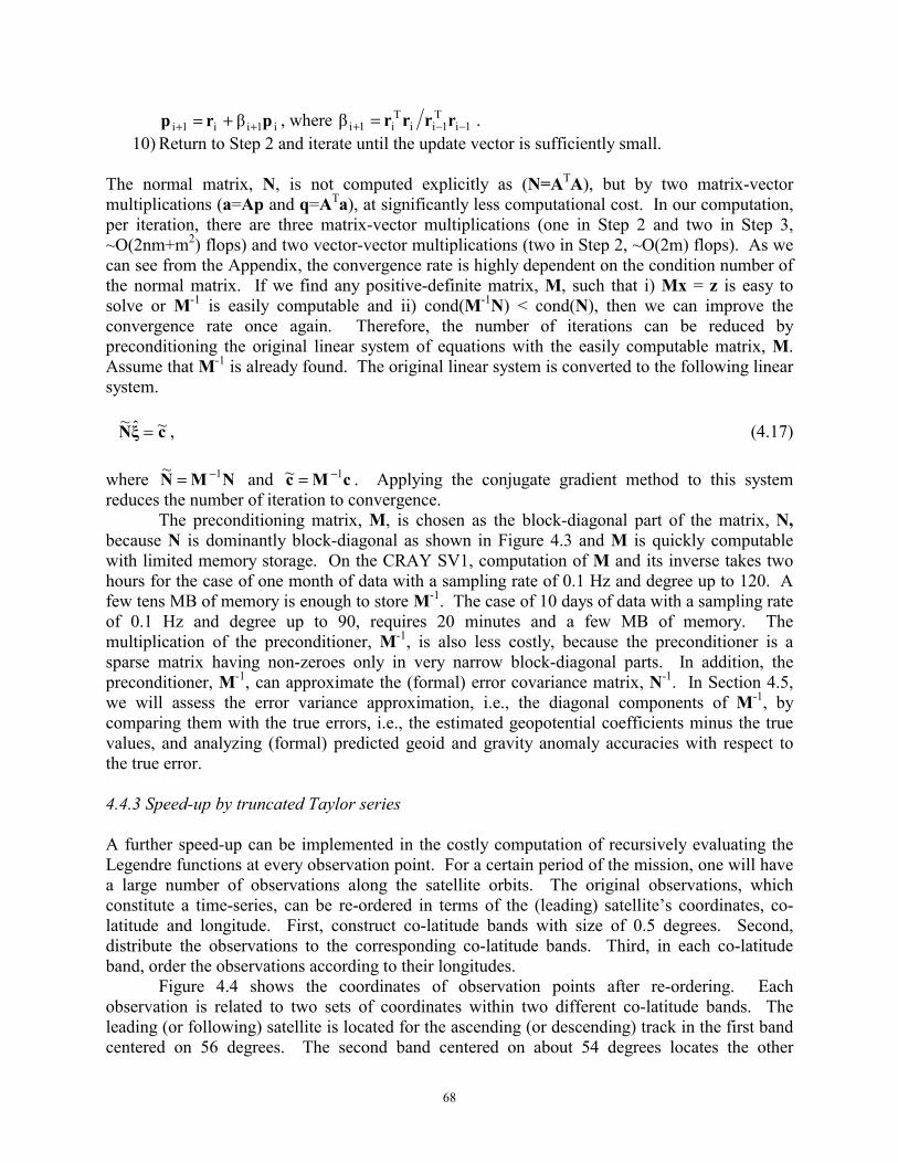
68

i1ii1i β prp ++ += , where 1iT

1iiTi1iβ −−+ = rrrr .

10) Return to Step 2 and iterate until the update vector is sufficiently small. The normal matrix, N, is not computed explicitly as (N=ATA), but by two matrix-vector multiplications (a=Ap and q=ATa), at significantly less computational cost. In our computation, per iteration, there are three matrix-vector multiplications (one in Step 2 and two in Step 3, ~O(2nm+m2) flops) and two vector-vector multiplications (two in Step 2, ~O(2m) flops). As we can see from the Appendix, the convergence rate is highly dependent on the condition number of the normal matrix. If we find any positive-definite matrix, M, such that i) Mx = z is easy to solve or M-1 is easily computable and ii) cond(M-1N) < cond(N), then we can improve the convergence rate once again. Therefore, the number of iterations can be reduced by preconditioning the original linear system of equations with the easily computable matrix, M. Assume that M-1 is already found. The original linear system is converted to the following linear system.

cξN ~ˆ~ = , (4.17) where NMN 1~ −= and cMc 1~ −= . Applying the conjugate gradient method to this system reduces the number of iteration to convergence.

The preconditioning matrix, M, is chosen as the block-diagonal part of the matrix, N, because N is dominantly block-diagonal as shown in Figure 4.3 and M is quickly computable with limited memory storage. On the CRAY SV1, computation of M and its inverse takes two hours for the case of one month of data with a sampling rate of 0.1 Hz and degree up to 120. A few tens MB of memory is enough to store M-1. The case of 10 days of data with a sampling rate of 0.1 Hz and degree up to 90, requires 20 minutes and a few MB of memory. The multiplication of the preconditioner, M-1, is also less costly, because the preconditioner is a sparse matrix having non-zeroes only in very narrow block-diagonal parts. In addition, the preconditioner, M-1, can approximate the (formal) error covariance matrix, N-1. In Section 4.5, we will assess the error variance approximation, i.e., the diagonal components of M-1, by comparing them with the true errors, i.e., the estimated geopotential coefficients minus the true values, and analyzing (formal) predicted geoid and gravity anomaly accuracies with respect to the true error. 4.4.3 Speed-up by truncated Taylor series A further speed-up can be implemented in the costly computation of recursively evaluating the Legendre functions at every observation point. For a certain period of the mission, one will have a large number of observations along the satellite orbits. The original observations, which constitute a time-series, can be re-ordered in terms of the (leading) satellite’s coordinates, co-latitude and longitude. First, construct co-latitude bands with size of 0.5 degrees. Second, distribute the observations to the corresponding co-latitude bands. Third, in each co-latitude band, order the observations according to their longitudes. Figure 4.4 shows the coordinates of observation points after re-ordering. Each observation is related to two sets of coordinates within two different co-latitude bands. The leading (or following) satellite is located for the ascending (or descending) track in the first band centered on 56 degrees. The second band centered on about 54 degrees locates the other

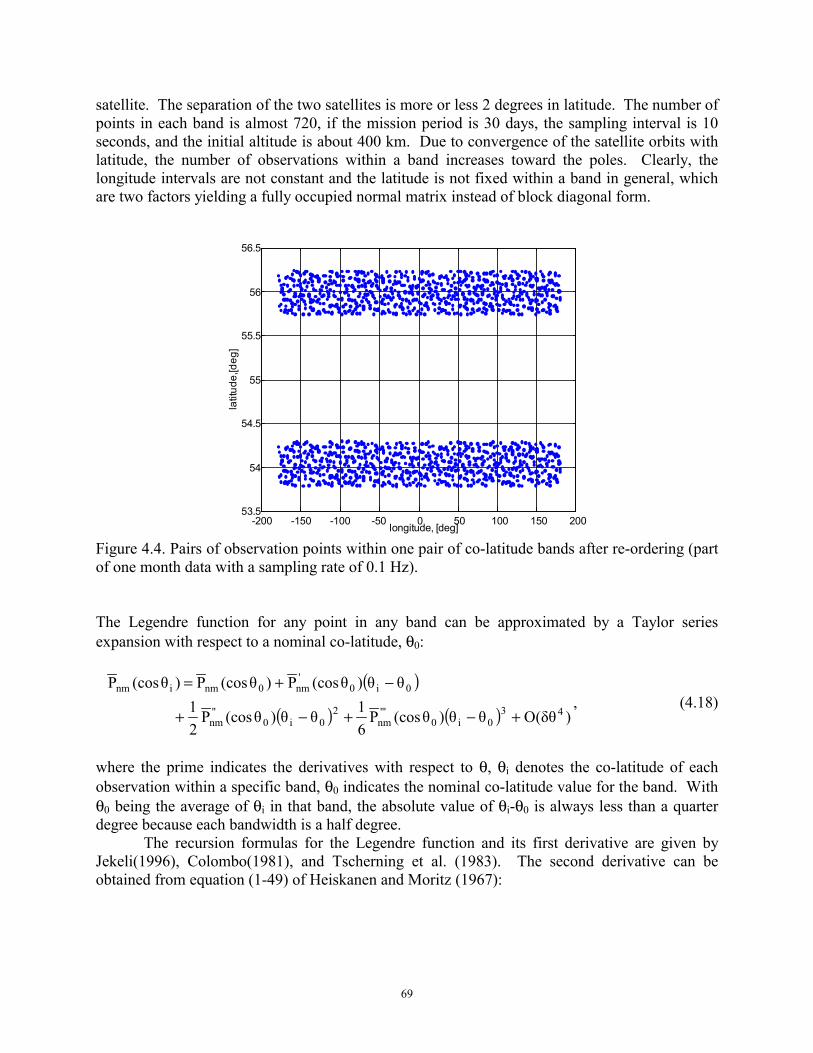
69

satellite. The separation of the two satellites is more or less 2 degrees in latitude. The number of points in each band is almost 720, if the mission period is 30 days, the sampling interval is 10 seconds, and the initial altitude is about 400 km. Due to convergence of the satellite orbits with latitude, the number of observations within a band increases toward the poles. Clearly, the longitude intervals are not constant and the latitude is not fixed within a band in general, which are two factors yielding a fully occupied normal matrix instead of block diagonal form.

-200 -150 -100 -50 0 50 100 150 200 53.5

54

54.5

55

55.5

56

56.5

longitude, [deg]

latit

ude,

[deg

]

Figure 4.4. Pairs of observation points within one pair of co-latitude bands after re-ordering (part of one month data with a sampling rate of 0.1 Hz). The Legendre function for any point in any band can be approximated by a Taylor series expansion with respect to a nominal co-latitude, θ0:

( )

( ) ( ) )δθ(Oθθ)θ(cosP61θθ)θ(cosP

21

θθ)θ(cosP)θ(cosP)θ(cosP

430i0

'''nm

20i0

''nm

0i0'nm0nminm

+−+−+

−+=, (4.18)

where the prime indicates the derivatives with respect to θ, θi denotes the co-latitude of each observation within a specific band, θ0 indicates the nominal co-latitude value for the band. With θ0 being the average of θi in that band, the absolute value of θi-θ0 is always less than a quarter degree because each bandwidth is a half degree. The recursion formulas for the Legendre function and its first derivative are given by Jekeli(1996), Colombo(1981), and Tscherning et al. (1983). The second derivative can be obtained from equation (1-49) of Heiskanen and Moritz (1967):

70

)θ(cosPtanθ

1)θ(cosPθsin

m1)n(n)θ(cosP 'nmnm2

2''

nm −

−+−= . (4.19)

The third derivative is obtained by differentiating (4.19).

)θ(cosPθsin1m1)n(n

tanθ1)θ(cosP

θsinθcos3m

tanθ1)n(n)θ(cosP '

nm2

2

nm3

2'''

nm

+++−+

−+= . (4.20)

Using (4.19) and (4.20), equation (4.18) can be written as:

)δθ(O

)θθ()θ(cosPθsin

1m1)n(ntanθ

1)θ(cosPθsinθcos3m

tanθ1)n(n

61

)θθ()θ(cosPtanθ

1)θ(cosPθsin

m1)n(n21

)θθ)(θ(cosP)θ(cosP)θ(cosP

4

30i0

'nm

02

2

00nm

03

02

0

20i0

'nm

00nm

02

2

0i0'nm0nminm

+

−

+++−+

−++

−

−+

++−+

−+=

(4.21)

By using this approximate formula for the Legendre function, one evaluates the function and its first derivative at the representative co-latitude, only once for each band. The total computation time is reduced significantly compared to the time required for the exact recursive evaluations of Legendre functions at every point. For the case of 10 days of data with a sampling rate of 0.1 Hz and degree up to 90, the computation time was reduced by more than one order of magnitude using (4.21). However, one commits a systematic error (algorithm error) by truncating the infinite Taylor series. Adding more higher-order terms could reduce this error below the level of instrument noise. Up to the third order, the level of algorithm error is ~10-5 m2/s2, which is two orders of magnitude less than the expected potential difference error (10-3 m2/s2) for the GRACE mission. Figure 4.5 shows the difference between the exact values of T12 and the values computed using the Taylor series up to the third order for one day. The error increases away from the nominal co-latitude (0.5°) and the overall error level is 10-5 m2/s2 (RMS). Therefore, we can use (4.21) for this study with negligible error.

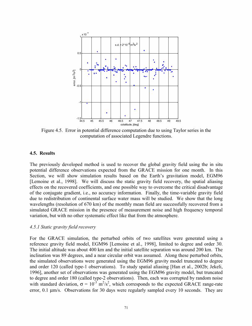
71

44.5 45 45.5 46 46.5 47 47.5 48 48.5 49 49.5 -1.5

-1

-0.5

0

0.5

1 x 10

-4

erro

r, [m

2 /s 2

]

colatitude, [deg]

s.d. = 2*10 -5 m2/s 2

Figure 4.5. Error in potential difference computation due to using Taylor series in the

computation of associated Legendre functions. 4.5. Results The previously developed method is used to recover the global gravity field using the in situ potential difference observations expected from the GRACE mission for one month. In this Section, we will show simulation results based on the Earth’s gravitation model, EGM96 [Lemoine et al., 1998]. We will discuss the static gravity field recovery, the spatial aliasing effects on the recovered coefficients, and one possible way to overcome the critical disadvantage of the conjugate gradient, i.e., no accuracy information. Finally, the time-variable gravity field due to redistribution of continental surface water mass will be studied. We show that the long wavelengths (resolution of 670 km) of the monthly mean field are successfully recovered from a simulated GRACE mission in the presence of measurement noise and high frequency temporal variation, but with no other systematic effect like that from the atmosphere. 4.5.1 Static gravity field recovery For the GRACE simulation, the perturbed orbits of two satellites were generated using a reference gravity field model, EGM96 [Lemoine et al., 1998], limited to degree and order 30. The initial altitude was about 400 km and the initial satellite separation was around 200 km. The inclination was 89 degrees, and a near circular orbit was assumed. Along these perturbed orbits, the simulated observations were generated using the EGM96 gravity model truncated to degree and order 120 (called type-1 observations). To study spatial aliasing [Han et al., 2002b; Jekeli, 1996], another set of observations was generated using the EGM96 gravity model, but truncated to degree and order 180 (called type-2 observations). Then, each was corrupted by random noise with standard deviation, σ = 10-3 m2/s2, which corresponds to the expected GRACE range-rate error, 0.1 µm/s. Observations for 30 days were regularly sampled every 10 seconds. They are

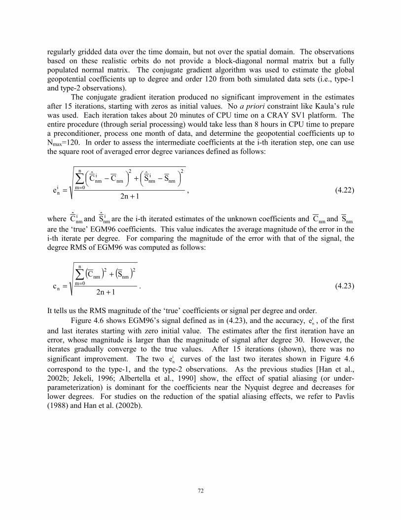
72

regularly gridded data over the time domain, but not over the spatial domain. The observations based on these realistic orbits do not provide a block-diagonal normal matrix but a fully populated normal matrix. The conjugate gradient algorithm was used to estimate the global geopotential coefficients up to degree and order 120 from both simulated data sets (i.e., type-1 and type-2 observations).

The conjugate gradient iteration produced no significant improvement in the estimates after 15 iterations, starting with zeros as initial values. No a priori constraint like Kaula’s rule was used. Each iteration takes about 20 minutes of CPU time on a CRAY SV1 platform. The entire procedure (through serial processing) would take less than 8 hours in CPU time to prepare a preconditioner, process one month of data, and determine the geopotential coefficients up to Nmax=120. In order to assess the intermediate coefficients at the i-th iteration step, one can use the square root of averaged error degree variances defined as follows:

12n

SSCCe

n

0m

2

nminm

2

nminm

in +

−+

−

=∑= , (4.22)

where inmC and i

nmS are the i-th iterated estimates of the unknown coefficients and nmC and nmS are the ‘true’ EGM96 coefficients. This value indicates the average magnitude of the error in the i-th iterate per degree. For comparing the magnitude of the error with that of the signal, the degree RMS of EGM96 was computed as follows:

( ) ( )12n

SCc

n

0m

2nm

2nm

n +

+=∑= . (4.23)

It tells us the RMS magnitude of the ‘true’ coefficients or signal per degree and order.

Figure 4.6 shows EGM96’s signal defined as in (4.23), and the accuracy, ine , of the first

and last iterates starting with zero initial value. The estimates after the first iteration have an error, whose magnitude is larger than the magnitude of signal after degree 30. However, the iterates gradually converge to the true values. After 15 iterations (shown), there was no significant improvement. The two i

ne curves of the last two iterates shown in Figure 4.6 correspond to the type-1, and the type-2 observations. As the previous studies [Han et al., 2002b; Jekeli, 1996; Albertella et al., 1990] show, the effect of spatial aliasing (or under-parameterization) is dominant for the coefficients near the Nyquist degree and decreases for lower degrees. For studies on the reduction of the spatial aliasing effects, we refer to Pavlis (1988) and Han et al. (2002b).

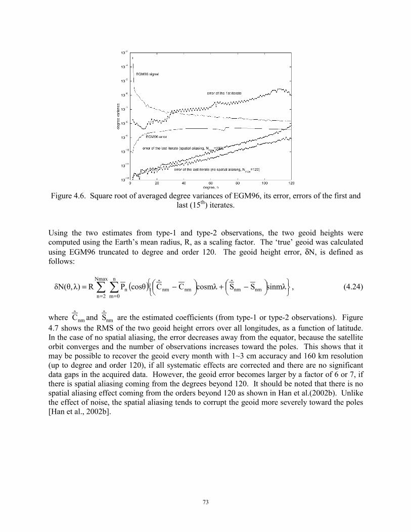
73

Figure 4.6. Square root of averaged degree variances of EGM96, its error, errors of the first and

last (15th) iterates. Using the two estimates from type-1 and type-2 observations, the two geoid heights were computed using the Earth’s mean radius, R, as a scaling factor. The ‘true’ geoid was calculated using EGM96 truncated to degree and order 120. The geoid height error, δN, is defined as follows:

( )

−+

−= ∑ ∑

= =sinmλSScosmλCCcosθPRλ)δN(θ, nmnmnmnm

Nmax

2n

n

0mn , (4.24)

where nmC and nmS are the estimated coefficients (from type-1 or type-2 observations). Figure 4.7 shows the RMS of the two geoid height errors over all longitudes, as a function of latitude. In the case of no spatial aliasing, the error decreases away from the equator, because the satellite orbit converges and the number of observations increases toward the poles. This shows that it may be possible to recover the geoid every month with 1~3 cm accuracy and 160 km resolution (up to degree and order 120), if all systematic effects are corrected and there are no significant data gaps in the acquired data. However, the geoid error becomes larger by a factor of 6 or 7, if there is spatial aliasing coming from the degrees beyond 120. It should be noted that there is no spatial aliasing effect coming from the orders beyond 120 as shown in Han et al.(2002b). Unlike the effect of noise, the spatial aliasing tends to corrupt the geoid more severely toward the poles [Han et al., 2002b].

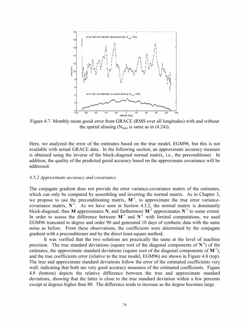
74

Figure 4.7. Monthly mean geoid error from GRACE (RMS over all longitudes) with and without

the spatial aliasing (Nmax is same as in (4.24)). Here, we analyzed the error of the estimates based on the true model, EGM96, but this is not available with actual GRACE data. In the following section, an approximate accuracy measure is obtained using the inverse of the block-diagonal normal matrix, i.e., the preconditioner. In addition, the quality of the predicted geoid accuracy based on the approximate covariance will be addressed. 4.5.2 Approximate accuracy and covariance The conjugate gradient does not provide the error variance-covariance matrix of the estimates, which can only be computed by assembling and inverting the normal matrix. As in Chapter 3, we propose to use the preconditioning matrix, M-1, to approximate the true error variance-covariance matrix, N-1. As we have seen in Section 4.3.2, the normal matrix is dominantly block-diagonal, thus M approximates N, and furthermore M-1 approximates N-1 to some extent. In order to assess the difference between M-1 and N-1 with limited computations, we used EGM96 truncated to degree and order 90 and generated 10 days of synthetic data with the same noise as before. From these observations, the coefficients were determined by the conjugate gradient with a preconditioner and by the direct least-square method.

It was verified that the two solutions are practically the same at the level of machine precision. The true standard deviations (square root of the diagonal components of N-1) of the estimates, the approximate standard deviations (square root of the diagonal components of M-1), and the true coefficients error (relative to the true model, EGM96) are shown in Figure 4.8 (top). The true and approximate standard deviations follow the error of the estimated coefficients very well, indicating that both are very good accuracy measures of the estimated coefficients. Figure 4.8 (bottom) depicts the relative difference between the true and approximate standard deviations, showing that the latter is close to the true standard deviation within a few percents except at degrees higher than 80. The difference tends to increase as the degree becomes large.

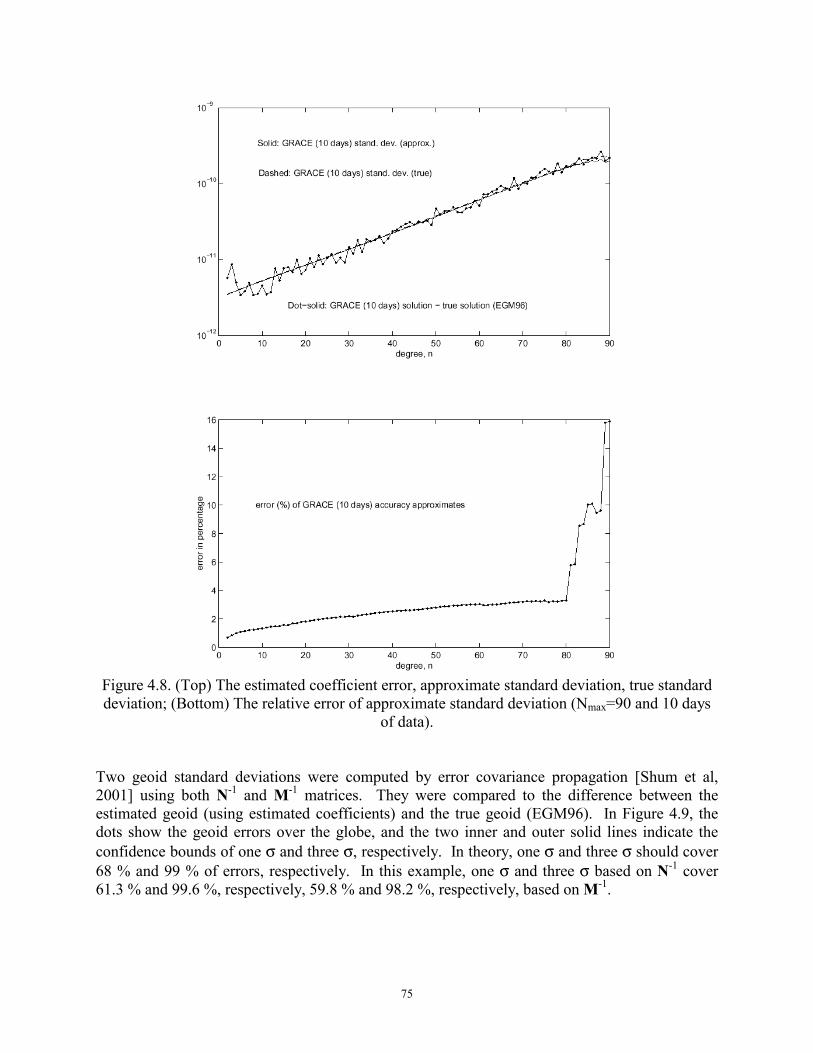
75

Figure 4.8. (Top) The estimated coefficient error, approximate standard deviation, true standard deviation; (Bottom) The relative error of approximate standard deviation (Nmax=90 and 10 days

of data). Two geoid standard deviations were computed by error covariance propagation [Shum et al, 2001] using both N-1 and M-1 matrices. They were compared to the difference between the estimated geoid (using estimated coefficients) and the true geoid (EGM96). In Figure 4.9, the dots show the geoid errors over the globe, and the two inner and outer solid lines indicate the confidence bounds of one σ and three σ, respectively. In theory, one σ and three σ should cover 68 % and 99 % of errors, respectively. In this example, one σ and three σ based on N-1 cover 61.3 % and 99.6 %, respectively, 59.8 % and 98.2 %, respectively, based on M-1.

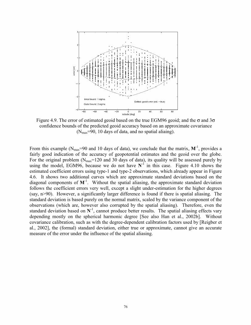
76

Figure 4.9. The error of estimated geoid based on the true EGM96 geoid; and the σ and 3σ

confidence bounds of the predicted geoid accuracy based on an approximate covariance (Nmax=90, 10 days of data, and no spatial aliaing).

From this example (Nmax=90 and 10 days of data), we conclude that the matrix, M-1, provides a fairly good indication of the accuracy of geopotential estimates and the geoid over the globe. For the original problem (Nmax=120 and 30 days of data), its quality will be assessed purely by using the model, EGM96, because we do not have N-1 in this case. Figure 4.10 shows the estimated coefficient errors using type-1 and type-2 observations, which already appear in Figure 4.6. It shows two additional curves which are approximate standard deviations based on the diagonal components of M-1. Without the spatial aliasing, the approximate standard deviation follows the coefficient errors very well, except a slight under-estimation for the higher degrees (say, n>90). However, a significantly larger difference is found if there is spatial aliasing. The standard deviation is based purely on the normal matrix, scaled by the variance component of the observations (which are, however also corrupted by the spatial aliasing). Therefore, even the standard deviation based on N-1, cannot produce better results. The spatial aliasing effects vary depending mostly on the spherical harmonic degree [See also Han et al., 2002b]. Without covariance calibration, such as with the degree-dependent calibration factors used by [Reigber et al., 2002], the (formal) standard deviation, either true or approximate, cannot give an accurate measure of the error under the influence of the spatial aliasing.

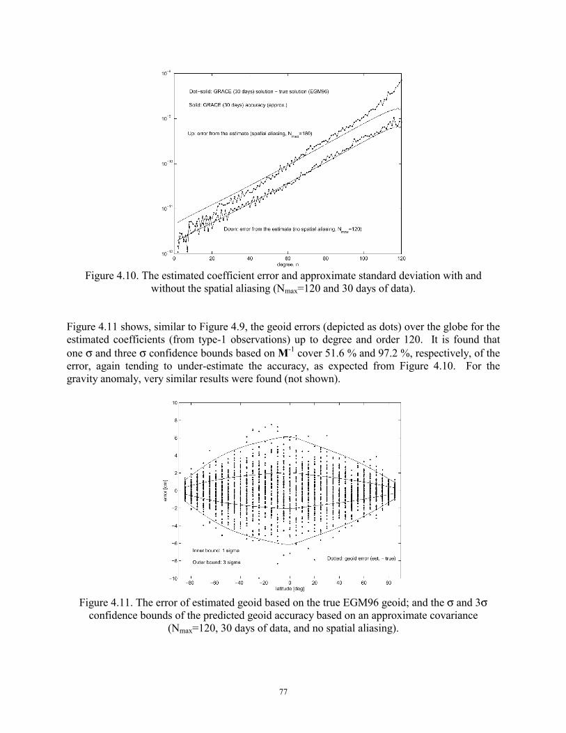
77

Figure 4.10. The estimated coefficient error and approximate standard deviation with and

without the spatial aliasing (Nmax=120 and 30 days of data). Figure 4.11 shows, similar to Figure 4.9, the geoid errors (depicted as dots) over the globe for the estimated coefficients (from type-1 observations) up to degree and order 120. It is found that one σ and three σ confidence bounds based on M-1 cover 51.6 % and 97.2 %, respectively, of the error, again tending to under-estimate the accuracy, as expected from Figure 4.10. For the gravity anomaly, very similar results were found (not shown).

Figure 4.11. The error of estimated geoid based on the true EGM96 geoid; and the σ and 3σ

confidence bounds of the predicted geoid accuracy based on an approximate covariance (Nmax=120, 30 days of data, and no spatial aliasing).

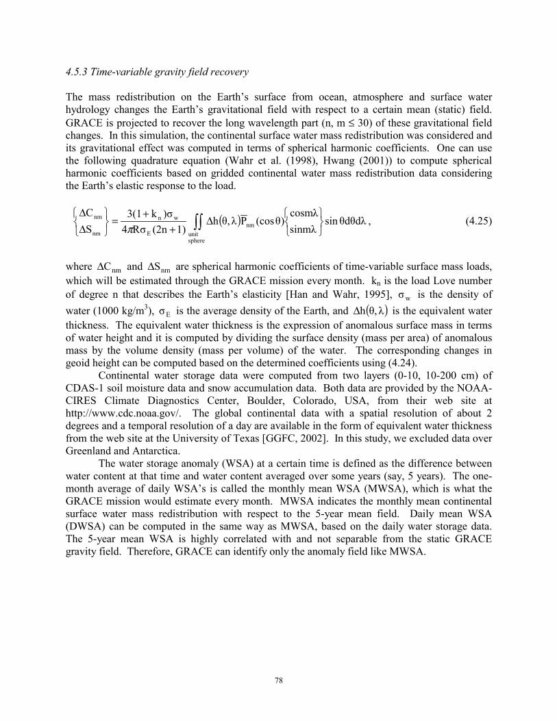
78

4.5.3 Time-variable gravity field recovery The mass redistribution on the Earth’s surface from ocean, atmosphere and surface water hydrology changes the Earth’s gravitational field with respect to a certain mean (static) field. GRACE is projected to recover the long wavelength part (n, m ≤ 30) of these gravitational field changes. In this simulation, the continental surface water mass redistribution was considered and its gravitational effect was computed in terms of spherical harmonic coefficients. One can use the following quadrature equation (Wahr et al. (1998), Hwang (2001)) to compute spherical harmonic coefficients based on gridded continental water mass redistribution data considering the Earth’s elastic response to the load.

( )∫∫

∆+

+=

∆∆

sphereunit

nmE

wn

nm

nm θdθdλsinsinmλcosmλ

)θ(cosPλθ,h1)(2nRσ4

)σk3(1SC

π, (4.25)

where nmC∆ and nmS∆ are spherical harmonic coefficients of time-variable surface mass loads, which will be estimated through the GRACE mission every month. kn is the load Love number of degree n that describes the Earth’s elasticity [Han and Wahr, 1995], wσ is the density of water (1000 kg/m3), Eσ is the average density of the Earth, and ( )λθ,h∆ is the equivalent water thickness. The equivalent water thickness is the expression of anomalous surface mass in terms of water height and it is computed by dividing the surface density (mass per area) of anomalous mass by the volume density (mass per volume) of the water. The corresponding changes in geoid height can be computed based on the determined coefficients using (4.24).

Continental water storage data were computed from two layers (0-10, 10-200 cm) of CDAS-1 soil moisture data and snow accumulation data. Both data are provided by the NOAA-CIRES Climate Diagnostics Center, Boulder, Colorado, USA, from their web site at http://www.cdc.noaa.gov/. The global continental data with a spatial resolution of about 2 degrees and a temporal resolution of a day are available in the form of equivalent water thickness from the web site at the University of Texas [GGFC, 2002]. In this study, we excluded data over Greenland and Antarctica.

The water storage anomaly (WSA) at a certain time is defined as the difference between water content at that time and water content averaged over some years (say, 5 years). The one-month average of daily WSA’s is called the monthly mean WSA (MWSA), which is what the GRACE mission would estimate every month. MWSA indicates the monthly mean continental surface water mass redistribution with respect to the 5-year mean field. Daily mean WSA (DWSA) can be computed in the same way as MWSA, based on the daily water storage data. The 5-year mean WSA is highly correlated with and not separable from the static GRACE gravity field. Therefore, GRACE can identify only the anomaly field like MWSA.

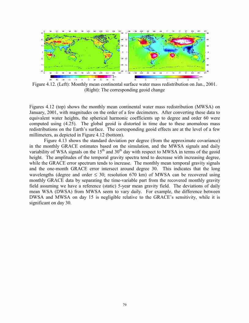
79

Figure 4.12. (Left): Monthly mean continental surface water mass redistribution on Jan., 2001.

(Right): The corresponding geoid change Figures 4.12 (top) shows the monthly mean continental water mass redistribution (MWSA) on January, 2001, with magnitudes on the order of a few decimeters. After converting these data to equivalent water heights, the spherical harmonic coefficients up to degree and order 60 were computed using (4.25). The global geoid is distorted in time due to these anomalous mass redistributions on the Earth’s surface. The corresponding geoid effects are at the level of a few millimeters, as depicted in Figure 4.12 (bottom).

Figure 4.13 shows the standard deviation per degree (from the approximate covariance) in the monthly GRACE estimates based on the simulation, and the MWSA signals and daily variability of WSA signals on the 15th and 30th day with respect to MWSA in terms of the geoid height. The amplitudes of the temporal gravity spectra tend to decrease with increasing degree, while the GRACE error spectrum tends to increase. The monthly mean temporal gravity signals and the one-month GRACE error intersect around degree 30. This indicates that the long wavelengths (degree and order ≤ 30; resolution 670 km) of MWSA can be recovered using monthly GRACE data by separating the time-variable part from the recovered monthly gravity field assuming we have a reference (static) 5-year mean gravity field. The deviations of daily mean WSA (DWSA) from MWSA seem to vary daily. For example, the difference between DWSA and MWSA on day 15 is negligible relative to the GRACE’s sensitivity, while it is significant on day 30.

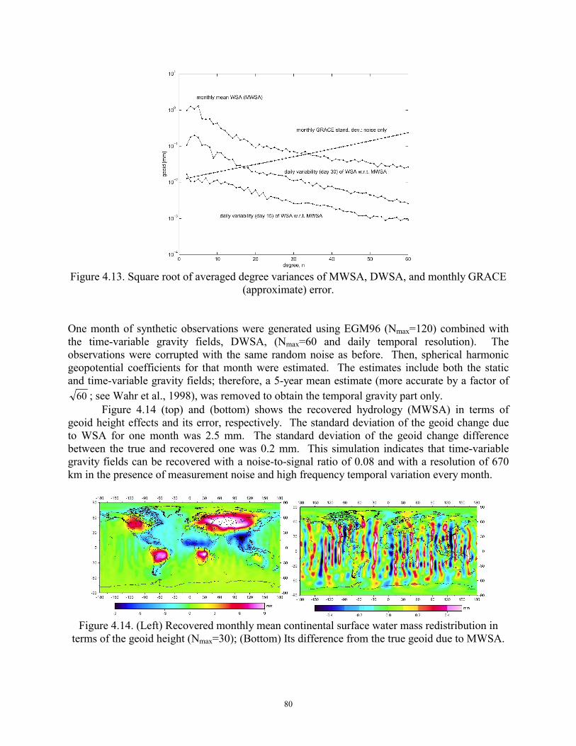
80

Figure 4.13. Square root of averaged degree variances of MWSA, DWSA, and monthly GRACE

(approximate) error. One month of synthetic observations were generated using EGM96 (Nmax=120) combined with the time-variable gravity fields, DWSA, (Nmax=60 and daily temporal resolution). The observations were corrupted with the same random noise as before. Then, spherical harmonic geopotential coefficients for that month were estimated. The estimates include both the static and time-variable gravity fields; therefore, a 5-year mean estimate (more accurate by a factor of

60 ; see Wahr et al., 1998), was removed to obtain the temporal gravity part only. Figure 4.14 (top) and (bottom) shows the recovered hydrology (MWSA) in terms of geoid height effects and its error, respectively. The standard deviation of the geoid change due to WSA for one month was 2.5 mm. The standard deviation of the geoid change difference between the true and recovered one was 0.2 mm. This simulation indicates that time-variable gravity fields can be recovered with a noise-to-signal ratio of 0.08 and with a resolution of 670 km in the presence of measurement noise and high frequency temporal variation every month.

Figure 4.14. (Left) Recovered monthly mean continental surface water mass redistribution in

terms of the geoid height (Nmax=30); (Bottom) Its difference from the true geoid due to MWSA.

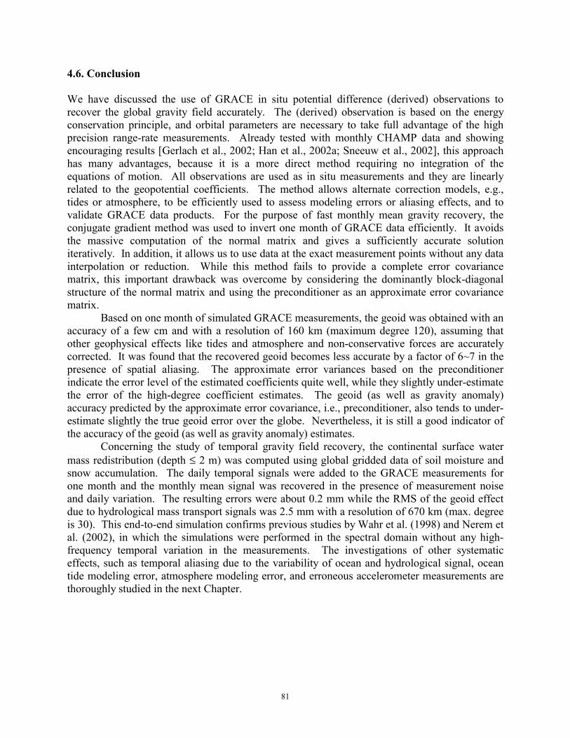
81

4.6. Conclusion We have discussed the use of GRACE in situ potential difference (derived) observations to recover the global gravity field accurately. The (derived) observation is based on the energy conservation principle, and orbital parameters are necessary to take full advantage of the high precision range-rate measurements. Already tested with monthly CHAMP data and showing encouraging results [Gerlach et al., 2002; Han et al., 2002a; Sneeuw et al., 2002], this approach has many advantages, because it is a more direct method requiring no integration of the equations of motion. All observations are used as in situ measurements and they are linearly related to the geopotential coefficients. The method allows alternate correction models, e.g., tides or atmosphere, to be efficiently used to assess modeling errors or aliasing effects, and to validate GRACE data products. For the purpose of fast monthly mean gravity recovery, the conjugate gradient method was used to invert one month of GRACE data efficiently. It avoids the massive computation of the normal matrix and gives a sufficiently accurate solution iteratively. In addition, it allows us to use data at the exact measurement points without any data interpolation or reduction. While this method fails to provide a complete error covariance matrix, this important drawback was overcome by considering the dominantly block-diagonal structure of the normal matrix and using the preconditioner as an approximate error covariance matrix. Based on one month of simulated GRACE measurements, the geoid was obtained with an accuracy of a few cm and with a resolution of 160 km (maximum degree 120), assuming that other geophysical effects like tides and atmosphere and non-conservative forces are accurately corrected. It was found that the recovered geoid becomes less accurate by a factor of 6~7 in the presence of spatial aliasing. The approximate error variances based on the preconditioner indicate the error level of the estimated coefficients quite well, while they slightly under-estimate the error of the high-degree coefficient estimates. The geoid (as well as gravity anomaly) accuracy predicted by the approximate error covariance, i.e., preconditioner, also tends to under-estimate slightly the true geoid error over the globe. Nevertheless, it is still a good indicator of the accuracy of the geoid (as well as gravity anomaly) estimates.

Concerning the study of temporal gravity field recovery, the continental surface water mass redistribution (depth ≤ 2 m) was computed using global gridded data of soil moisture and snow accumulation. The daily temporal signals were added to the GRACE measurements for one month and the monthly mean signal was recovered in the presence of measurement noise and daily variation. The resulting errors were about 0.2 mm while the RMS of the geoid effect due to hydrological mass transport signals was 2.5 mm with a resolution of 670 km (max. degree is 30). This end-to-end simulation confirms previous studies by Wahr et al. (1998) and Nerem et al. (2002), in which the simulations were performed in the spectral domain without any high-frequency temporal variation in the measurements. The investigations of other systematic effects, such as temporal aliasing due to the variability of ocean and hydrological signal, ocean tide modeling error, atmosphere modeling error, and erroneous accelerometer measurements are thoroughly studied in the next Chapter.

82

5. TIME-VARIABLE EFFECTS OF OCEAN TIDES, ATMOSPHERE, AND CONTINENTAL WATER MASS ON MONTHLY MEAN GRACE GRAVITY FIELD

5.1. Introduction It is expected that GRACE will be sensitive to monthly averaged time-varying mass distributions of the Earth system and that these climate-sensitive signals will be measured with sub-centimeter accuracy in units of column of water movement near Earth’s surface with a spatial resolution of 250 km or longer.

Wahr et al (1998) and Han et al. (2003) demonstrated the successful recovery of continental surface water hydrology with an accuracy of a few mm in the equivalent water height and a resolution of a few hundred kilometers. Han et al. (2003) and Nerem et al. (2002) also demonstrated the successful recovery of ocean mass redistribution with more or less the same accuracy and similar spatial resolution. For the recovery of temporal gravity fields, the two largest systematic and high (temporal) frequency phenomena, ocean tides and atmosphere, must be first modeled and removed from GRACE observables. This removal is based on the currently available models, e.g., CSR4.0 [Eanes and Bettadpur, 1995] or NAO99 [Matsumoto et al., 2000] for the ocean tide, ECMWF [European Centre for Medium-range Weather Forecast, 1995] or NCEP [Kalnay et al., 1996] for the atmosphere. The difference between (or error in) these models would produce errors in computing tidal and atmospheric effects on the satellite orbit, thus they would corrupt the recovered gravity fields. In addition, the limited time resolution of the gravity field products, i.e., every month, and the peculiar characteristics of the orbital sampling of GRACE satellites induce high frequency temporal aliasing effects on the monthly mean gravity products. That is, the short period temporal mass variations due to the residual (remaining) ocean tides, residual atmosphere, and continental water mass would alias into the longer period components and systematically contaminate the monthly mean gravity field estimates.

Unfortunately, none of the previous studies really deal with the temporal aliasing problem in the recovered monthly gravity coefficients. Simulations such as by Wahr et al. (1998) and Nerem et al. (2002), started with spherical harmonic coefficients for ocean and continental surface water hydrology based on the reference models. Then, random noise was added to these coefficients according to the GRACE error degree variance model assuming independent errors among different order coefficients. Finally, spatial averaging was applied in a spectral domain to reduce errors coming from ill-determined higher degree and order coefficients, thus yielding accurate long wavelength estimates of temporal gravity. No inversion of GRACE data was involved in this approach, as mentioned in Wahr and Velicogna, (2002). It was limited to an analysis in the spectral domain and hardly represents the temporal aliasing problem existing in monthly mean gravity field estimates. The aliasing problem is associated with the complex GRACE orbital configuration and has not yet been well investigated in the previous analyses. As Velicogna et al. (2001) mentioned, the aliasing effects cannot be predicted without a detailed orbital simulation, because it is a complex output resulting from GRACE’s local sampling (in the space domain at every instant) for a month. Note that the temporal mass redistributions over some regions will not necessarily be incorporated into the monthly GRACE estimates because of the characteristic of GRACE’s orbital sampling.

In order to identify the realistic aliasing effects on the recovered gravity field, we simulated the perturbations due to the time-variable ocean tidal and atmospheric model errors

83

along the GRACE orbit for a month. Then we fully inverted one month of data to solve the geopotential coefficients up to the maximum degree and order 120 in the presence of the measurement noise and ocean tidal and atmospheric model error (or residual ocean tide and atmosphere). By investigating the recovered monthly gravity coefficient estimates and comparing them with estimates in the presence of measurement error only, we are able to analyze the time-variable residual tidal and atmospheric effects on the monthly mean gravity estimates. In the following sections, we will show the models and data used for the ocean tide, atmosphere, and continental surface water hydrology. An approximate method to generate the range-rate perturbations due to these temporal gravity signals will be presented and an efficient method to invert monthly GRACE data will be briefly addressed. We will present and analyze the detailed results on aliasing of residual ocean tide and atmosphere in both the spatial and spectral domains. Especially, the effect of daily variability of continental surface water hydrology on the monthly mean gravity estimates will be discussed. Finally, a possible way to reduce the aliasing effects on monthly mean field is suggested with some persuasive results. 5.2. Data and Method 5.2.1 Models for Ocean Tides As a possible indicator for the modeling error of ocean tides, the difference between two distinct tide models can be used. Here, we used the difference between a hydrodynamic model, NAO99 [Matsumoto et al., 2000] and the altimetry-based model, CSR4.0 [Eanes and Bettadpur, 1995]. Data for the models were provided by P. Knudsen at KMS, Denmark. This kind of tidal modeling error was studied recently Ray et al. (2001) and Knudsen and Anderson (2002) who computed the mean power spectra of ocean tide model differences and compared them to GRACE sensitivity. Ray et al. (2001) first initiated the problem in the M2 constituent’s modeling error affecting the GRACE gravity estimates. However, the tidal error and the GRACE sensitivity curves in those studies should not be compared to identify a possible corruption from the M2 constituent’s modeling error, because their time periods are not matched (12.4 hours averaging for M2 constituent error versus 3 months averaging for GRACE sensitivity). This study lacks the temporal variation effect of the tidal modeling error on the GRACE estimates, and actually no orbital sampling was involved. A subsequent and comparable analysis was performed by Knudsen and Anderson (2002) who computed the aliasing frequencies [Parke et al., 1987] for the four most energetic constituents. They tried to compute a monthly mean tidal error by applying convolution in a time domain using a block averaging function with a corresponding aliasing period. However, it still disregards the GRACE’s orbital sampling and lacks a full GRACE simulation and inversion.

In this study, the effects of the tidal model error, defined as difference between CSR4.0 and NAO99, were transformed into the GRACE range-rate and potential difference observables [Han et al., 2003]. By inverting these observables, the effects of their temporal variation on the monthly mean gravity field estimates were studied. The results were analyzed considering the orbital sampling and the periods of each constituent. This approach provides a more direct and appropriate assessment on the effect of the time-variable tidal error than the other limited analyses that avoid an orbital simulation and inversion.

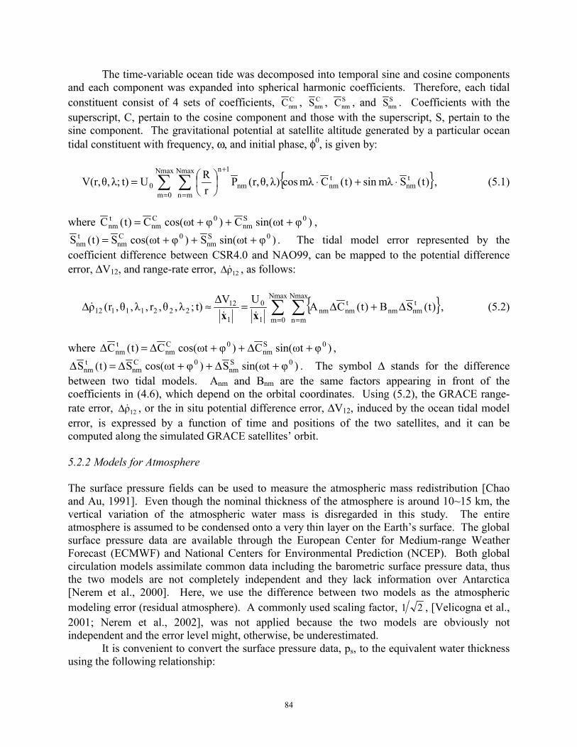
84

The time-variable ocean tide was decomposed into temporal sine and cosine components and each component was expanded into spherical harmonic coefficients. Therefore, each tidal constituent consist of 4 sets of coefficients, C

nmC , CnmS , S

nmC , and SnmS . Coefficients with the

superscript, C, pertain to the cosine component and those with the superscript, S, pertain to the sine component. The gravitational potential at satellite altitude generated by a particular ocean tidal constituent with frequency, ω, and initial phase, φ0, is given by:

{ })t(Smλsin)t(Cmλcos)λθ,r,(PrRUt)λ;θ,V(r, t

nmtnm

Nmax

0m

Nmax

mnnm

1n

0 ⋅+⋅

= ∑ ∑

= =

+

, (5.1)

where )φωtsin(C)φωtcos(C)t(C 0S

nm0C

nmtnm +++= ,

)φωtsin(S)φωtcos(S)t(S 0Snm

0Cnm

tnm +++= . The tidal model error represented by the

coefficient difference between CSR4.0 and NAO99, can be mapped to the potential difference error, ∆V12, and range-rate error, 12ρ&∆ , as follows:

{ }∑ ∑= =

∆+∆=∆

≈∆Nmax

0m

Nmax

mn

tnmnm

tnmnm

1

0

1

1222211112 )t(SB)t(CA

UVt);λ,θ,r,λ,θ,r(ρ

xx &&& , (5.2)

where )φωtsin(C)φωtcos(C)t(C 0S

nm0C

nmtnm +∆++∆=∆ ,

)φωtsin(S)φωtcos(S)t(S 0Snm

0Cnm

tnm +∆++∆=∆ . The symbol ∆ stands for the difference

between two tidal models. Anm and Bnm are the same factors appearing in front of the coefficients in (4.6), which depend on the orbital coordinates. Using (5.2), the GRACE range-rate error, 12ρ&∆ , or the in situ potential difference error, ∆V12, induced by the ocean tidal model error, is expressed by a function of time and positions of the two satellites, and it can be computed along the simulated GRACE satellites’ orbit. 5.2.2 Models for Atmosphere The surface pressure fields can be used to measure the atmospheric mass redistribution [Chao and Au, 1991]. Even though the nominal thickness of the atmosphere is around 10~15 km, the vertical variation of the atmospheric water mass is disregarded in this study. The entire atmosphere is assumed to be condensed onto a very thin layer on the Earth’s surface. The global surface pressure data are available through the European Center for Medium-range Weather Forecast (ECMWF) and National Centers for Environmental Prediction (NCEP). Both global circulation models assimilate common data including the barometric surface pressure data, thus the two models are not completely independent and they lack information over Antarctica [Nerem et al., 2000]. Here, we use the difference between two models as the atmospheric modeling error (residual atmosphere). A commonly used scaling factor, 21 , [Velicogna et al., 2001; Nerem et al., 2002], was not applied because the two models are obviously not independent and the error level might, otherwise, be underestimated.

It is convenient to convert the surface pressure data, ps, to the equivalent water thickness using the following relationship:

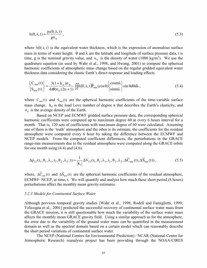
85

w

s

gσ)tλ,θ,(p)tλ,θ,(h = , (5.3)

where ( )tλ,θ,h is the equivalent water thickness, which is the expression of anomalous surface mass in terms of water height. θ and λ are the latitude and longitude of surface pressure data, t is time, g is the nominal gravity value, and wσ is the density of water (1000 kg/m3). We use the quadrature equation (as used by Wahr et al., 1998, and Hwang, 2001) to compute the spherical harmonic coefficients of atmospheric mass change based on the regular gridded equivalent water thickness data considering the elastic Earth’s direct response and loading effects.

( ) θdθdλsinsinmλcosmλ

)θ(cosPtλ,θ,h1)(2nRσ4

)σk3(1)t(S)t(C

nmE

wn

nm

nm

++

=

∫∫π, (5.4)

where )t(Cnm and t)(Snm are the spherical harmonic coefficients of the time-variable surface mass change. kn is the load Love number of degree n that describes the Earth’s elasticity, and

Eσ is the average density of the Earth. Based on NCEP and ECMWF gridded surface pressure data, the corresponding spherical

harmonic coefficients were computed up to maximum degree 60 at every 6 hours interval for a month. That is, 120 sets of coefficients with maximum degree of 60 were calculated. Assuming one of them is the ‘truth’ atmosphere and the other is its estimate, the coefficients for the residual atmosphere were computed every 6 hour by taking the difference between the ECMWF and NCEP models. From the computed coefficient differences, the perturbations in the GRACE range-rate measurements due to the residual atmosphere were computed along the GRACE orbits for one month using (4.4) and (4.6):

))t(S),t(C;λ,θ,r,λ,θ,r(V1t);λ,θ,r,λ,θ,r(ρ nmnm222111121

22211112 ∆∆∆≈∆x&

& , (5.5)

where, )t(Cnm∆ and )t(Snm∆ are the spherical harmonic coefficients of the residual atmosphere, ECMWF–NCEP, at time, t. We will quantify and analyze how much these short period (6 hours) perturbations affect the monthly mean gravity estimates. 5.2.3 Models for Continental Surface Water Although previous temporal gravity studies [Wahr et al., 1998; Rodell and Famiglietti, 1999; Velicogna et al., 2001] predicted the successful recovery of continental surface water mass from the GRACE mission, it is still questionable how much the variability of the surface water mass affects the monthly mean GRACE gravity field. Using a similar approach as for the atmosphere, the error due to the variability of the ground water mass can be quantified in the measurement domain as well as the spectral domain based on a certain model which can reasonably describe the short period variations of continental surface water.

The NCEP (National Centers for Environmental Prediction) / NCAR (National Center for Atmospheric Research) reanalysis project has been providing through the NOAA-CIRES

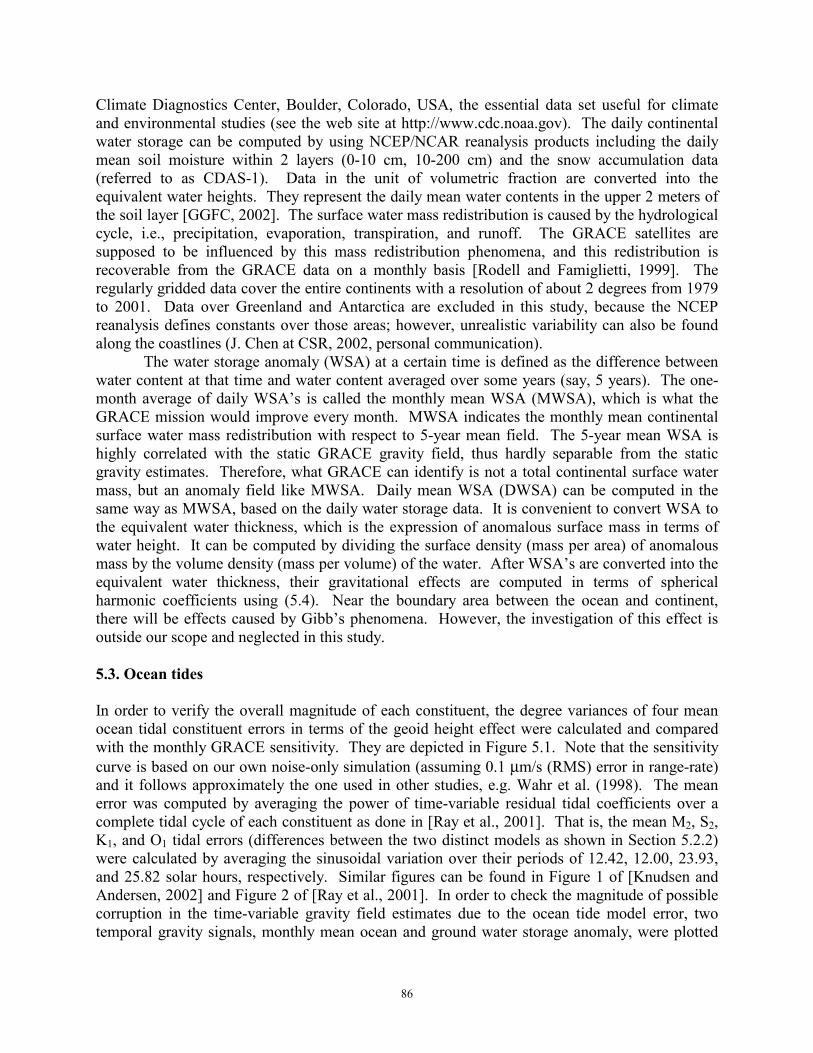
86

Climate Diagnostics Center, Boulder, Colorado, USA, the essential data set useful for climate and environmental studies (see the web site at http://www.cdc.noaa.gov). The daily continental water storage can be computed by using NCEP/NCAR reanalysis products including the daily mean soil moisture within 2 layers (0-10 cm, 10-200 cm) and the snow accumulation data (referred to as CDAS-1). Data in the unit of volumetric fraction are converted into the equivalent water heights. They represent the daily mean water contents in the upper 2 meters of the soil layer [GGFC, 2002]. The surface water mass redistribution is caused by the hydrological cycle, i.e., precipitation, evaporation, transpiration, and runoff. The GRACE satellites are supposed to be influenced by this mass redistribution phenomena, and this redistribution is recoverable from the GRACE data on a monthly basis [Rodell and Famiglietti, 1999]. The regularly gridded data cover the entire continents with a resolution of about 2 degrees from 1979 to 2001. Data over Greenland and Antarctica are excluded in this study, because the NCEP reanalysis defines constants over those areas; however, unrealistic variability can also be found along the coastlines (J. Chen at CSR, 2002, personal communication). The water storage anomaly (WSA) at a certain time is defined as the difference between water content at that time and water content averaged over some years (say, 5 years). The one-month average of daily WSA’s is called the monthly mean WSA (MWSA), which is what the GRACE mission would improve every month. MWSA indicates the monthly mean continental surface water mass redistribution with respect to 5-year mean field. The 5-year mean WSA is highly correlated with the static GRACE gravity field, thus hardly separable from the static gravity estimates. Therefore, what GRACE can identify is not a total continental surface water mass, but an anomaly field like MWSA. Daily mean WSA (DWSA) can be computed in the same way as MWSA, based on the daily water storage data. It is convenient to convert WSA to the equivalent water thickness, which is the expression of anomalous surface mass in terms of water height. It can be computed by dividing the surface density (mass per area) of anomalous mass by the volume density (mass per volume) of the water. After WSA’s are converted into the equivalent water thickness, their gravitational effects are computed in terms of spherical harmonic coefficients using (5.4). Near the boundary area between the ocean and continent, there will be effects caused by Gibb’s phenomena. However, the investigation of this effect is outside our scope and neglected in this study. 5.3. Ocean tides In order to verify the overall magnitude of each constituent, the degree variances of four mean ocean tidal constituent errors in terms of the geoid height effect were calculated and compared with the monthly GRACE sensitivity. They are depicted in Figure 5.1. Note that the sensitivity curve is based on our own noise-only simulation (assuming 0.1 µm/s (RMS) error in range-rate) and it follows approximately the one used in other studies, e.g. Wahr et al. (1998). The mean error was computed by averaging the power of time-variable residual tidal coefficients over a complete tidal cycle of each constituent as done in [Ray et al., 2001]. That is, the mean M2, S2, K1, and O1 tidal errors (differences between the two distinct models as shown in Section 5.2.2) were calculated by averaging the sinusoidal variation over their periods of 12.42, 12.00, 23.93, and 25.82 solar hours, respectively. Similar figures can be found in Figure 1 of [Knudsen and Andersen, 2002] and Figure 2 of [Ray et al., 2001]. In order to check the magnitude of possible corruption in the time-variable gravity field estimates due to the ocean tide model error, two temporal gravity signals, monthly mean ocean and ground water storage anomaly, were plotted

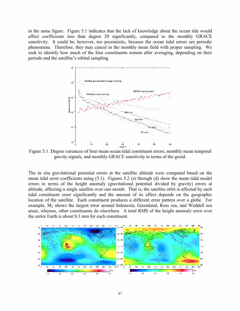
87

in the same figure. Figure 5.1 indicates that the lack of knowledge about the ocean tide would affect coefficients less than degree 20 significantly, compared to the monthly GRACE sensitivity. It could be, however, too pessimistic, because the ocean tidal errors are periodic phenomena. Therefore, they may cancel in the monthly mean field with proper sampling. We seek to identify how much of the four constituents remain after averaging, depending on their periods and the satellite’s orbital sampling.

Figure 5.1. Degree variances of four mean ocean tidal constituent errors, monthly mean temporal

gravity signals, and monthly GRACE sensitivity in terms of the geoid. The in situ gravitational potential errors at the satellite altitude were computed based on the mean tidal error coefficients using (5.1). Figures 5.2 (a) through (d) show the mean tidal model errors in terms of the height anomaly (gravitational potential divided by gravity) errors at altitude, affecting a single satellite over one month. That is, the satellite orbit is affected by each tidal constituent error significantly and the amount of its effect depends on the geographic location of the satellite. Each constituent produces a different error pattern over a globe. For example, M2 shows the largest error around Indonesia, Greenland, Ross sea, and Weddell sea areas, whereas, other constituents do elsewhere. A total RMS of the height anomaly error over the entire Earth is about 0.3 mm for each constituent.

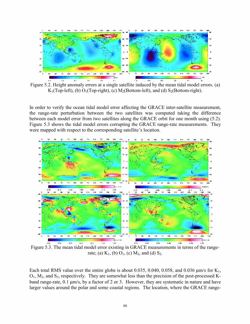
88

Figure 5.2. Height anomaly errors at a single satellite induced by the mean tidal model errors. (a)

K1(Top-left), (b) O1(Top-right), (c) M2(Bottom-left), and (d) S2(Bottom-right). In order to verify the ocean tidal model error affecting the GRACE inter-satellite measurement, the range-rate perturbation between the two satellites was computed taking the difference between each model error from two satellites along the GRACE orbit for one month using (5.2). Figure 5.3 shows the tidal model errors corrupting the GRACE range-rate measurements. They were mapped with respect to the corresponding satellite’s location.

Figure 5.3. The mean tidal model error existing in GRACE measurements in terms of the range-

rate; (a) K1, (b) O1, (c) M2, and (d) S2. Each total RMS value over the entire globe is about 0.035, 0.040, 0.058, and 0.036 µm/s for K1, O1, M2, and S2, respectively. They are somewhat less than the precision of the post-processed K-band range-rate, 0.1 µm/s, by a factor of 2 or 3. However, they are systematic in nature and have larger values around the polar and some coastal regions. The location, where the GRACE range-

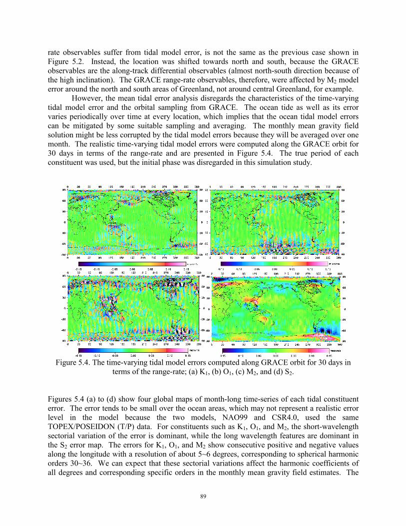
89

rate observables suffer from tidal model error, is not the same as the previous case shown in Figure 5.2. Instead, the location was shifted towards north and south, because the GRACE observables are the along-track differential observables (almost north-south direction because of the high inclination). The GRACE range-rate observables, therefore, were affected by M2 model error around the north and south areas of Greenland, not around central Greenland, for example. However, the mean tidal error analysis disregards the characteristics of the time-varying tidal model error and the orbital sampling from GRACE. The ocean tide as well as its error varies periodically over time at every location, which implies that the ocean tidal model errors can be mitigated by some suitable sampling and averaging. The monthly mean gravity field solution might be less corrupted by the tidal model errors because they will be averaged over one month. The realistic time-varying tidal model errors were computed along the GRACE orbit for 30 days in terms of the range-rate and are presented in Figure 5.4. The true period of each constituent was used, but the initial phase was disregarded in this simulation study.

Figure 5.4. The time-varying tidal model errors computed along GRACE orbit for 30 days in

terms of the range-rate; (a) K1, (b) O1, (c) M2, and (d) S2. Figures 5.4 (a) to (d) show four global maps of month-long time-series of each tidal constituent error. The error tends to be small over the ocean areas, which may not represent a realistic error level in the model because the two models, NAO99 and CSR4.0, used the same TOPEX/POSEIDON (T/P) data. For constituents such as K1, O1, and M2, the short-wavelength sectorial variation of the error is dominant, while the long wavelength features are dominant in the S2 error map. The errors for K1, O1, and M2 show consecutive positive and negative values along the longitude with a resolution of about 5~6 degrees, corresponding to spherical harmonic orders 30~36. We can expect that these sectorial variations affect the harmonic coefficients of all degrees and corresponding specific orders in the monthly mean gravity field estimates. The

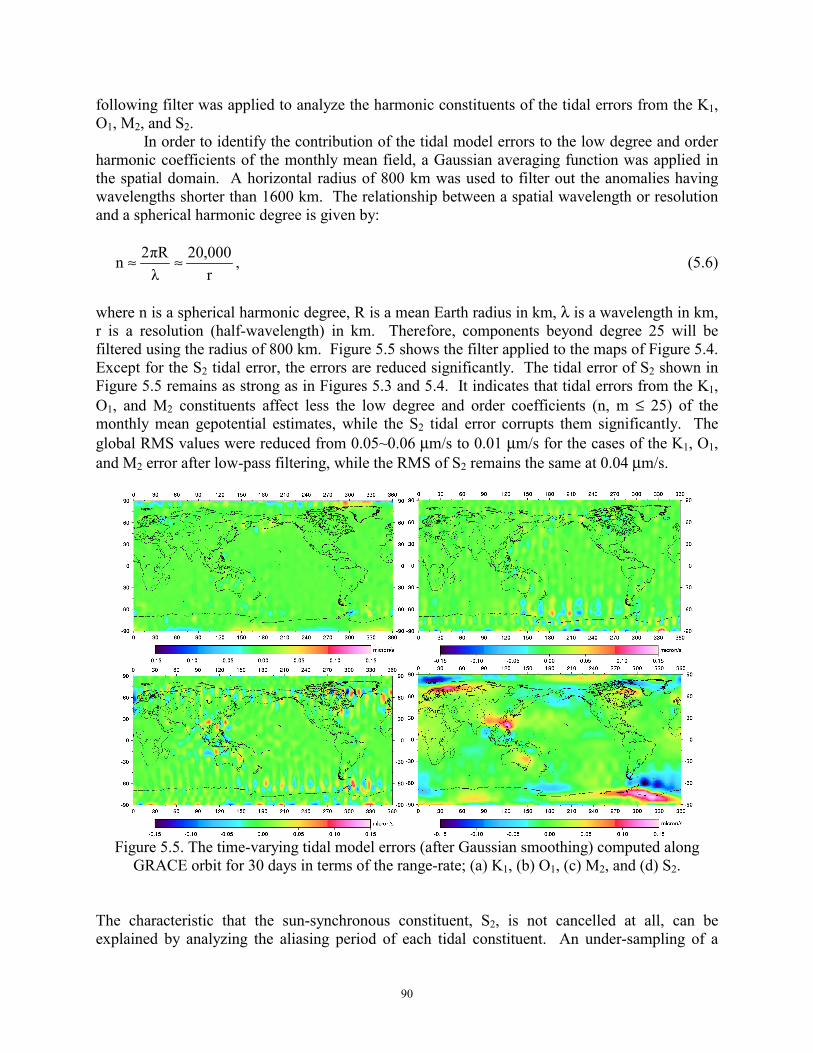
90

following filter was applied to analyze the harmonic constituents of the tidal errors from the K1, O1, M2, and S2. In order to identify the contribution of the tidal model errors to the low degree and order harmonic coefficients of the monthly mean field, a Gaussian averaging function was applied in the spatial domain. A horizontal radius of 800 km was used to filter out the anomalies having wavelengths shorter than 1600 km. The relationship between a spatial wavelength or resolution and a spherical harmonic degree is given by:

r000,20

λπR2n ≈≈ , (5.6)

where n is a spherical harmonic degree, R is a mean Earth radius in km, λ is a wavelength in km, r is a resolution (half-wavelength) in km. Therefore, components beyond degree 25 will be filtered using the radius of 800 km. Figure 5.5 shows the filter applied to the maps of Figure 5.4. Except for the S2 tidal error, the errors are reduced significantly. The tidal error of S2 shown in Figure 5.5 remains as strong as in Figures 5.3 and 5.4. It indicates that tidal errors from the K1, O1, and M2 constituents affect less the low degree and order coefficients (n, m ≤ 25) of the monthly mean gepotential estimates, while the S2 tidal error corrupts them significantly. The global RMS values were reduced from 0.05~0.06 µm/s to 0.01 µm/s for the cases of the K1, O1, and M2 error after low-pass filtering, while the RMS of S2 remains the same at 0.04 µm/s.

Figure 5.5. The time-varying tidal model errors (after Gaussian smoothing) computed along

GRACE orbit for 30 days in terms of the range-rate; (a) K1, (b) O1, (c) M2, and (d) S2. The characteristic that the sun-synchronous constituent, S2, is not cancelled at all, can be explained by analyzing the aliasing period of each tidal constituent. An under-sampling of a

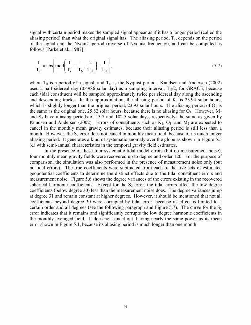
91

signal with certain period makes the sampled signal appear as if it has a longer period (called the aliasing period) than what the original signal has. The aliasing period, Ta, depends on the period of the signal and the Nyquist period (inverse of Nyquist frequency), and can be computed as follows [Parke et al., 1987]:

−

+=

NNNka T1

T2,

T1

T1modabs

T1 , (5.7)

where Tk is a period of a signal, and TN is the Nyquist period. Knudsen and Andersen (2002) used a half sidereal day (0.4986 solar day) as a sampling interval, TN/2, for GRACE, because each tidal constituent will be sampled approximately twice per sidereal day along the ascending and descending tracks. In this approximation, the aliasing period of K1 is 23.94 solar hours, which is slightly longer than the original period, 23.93 solar hours. The aliasing period of O1 is the same as the original one, 25.82 solar hours, because there is no aliasing for O1. However, M2 and S2 have aliasing periods of 13.7 and 182.5 solar days, respectively, the same as given by Knudsen and Andersen (2002). Errors of constituents such as K1, O1, and M2 are expected to cancel in the monthly mean gravity estimates, because their aliasing period is still less than a month. However, the S2 error does not cancel in monthly mean field, because of its much longer aliasing period. It generates a kind of systematic anomaly over the globe as shown in Figure 5.5 (d) with semi-annual characteristics in the temporal gravity field estimates. In the presence of these four systematic tidal model errors (but no measurement noise), four monthly mean gravity fields were recovered up to degree and order 120. For the purpose of comparison, the simulation was also performed in the presence of measurement noise only (but no tidal errors). The true coefficients were subtracted from each of the five sets of estimated geopotential coefficients to determine the distinct effects due to the tidal constituent errors and measurement noise. Figure 5.6 shows the degree variances of the errors existing in the recovered spherical harmonic coefficients. Except for the S2 error, the tidal errors affect the low degree coefficients (below degree 30) less than the measurement noise does. The degree variances jump at degree 31 and remain constant at higher degrees. However, it should be mentioned that not all coefficients beyond degree 30 were corrupted by tidal error, because its effect is limited to a certain order and all degrees (see the following paragraph and Figure 5.7). The curve for the S2 error indicates that it remains and significantly corrupts the low degree harmonic coefficients in the monthly averaged field. It does not cancel out, having nearly the same power as its mean error shown in Figure 5.1, because its aliasing period is much longer than one month.

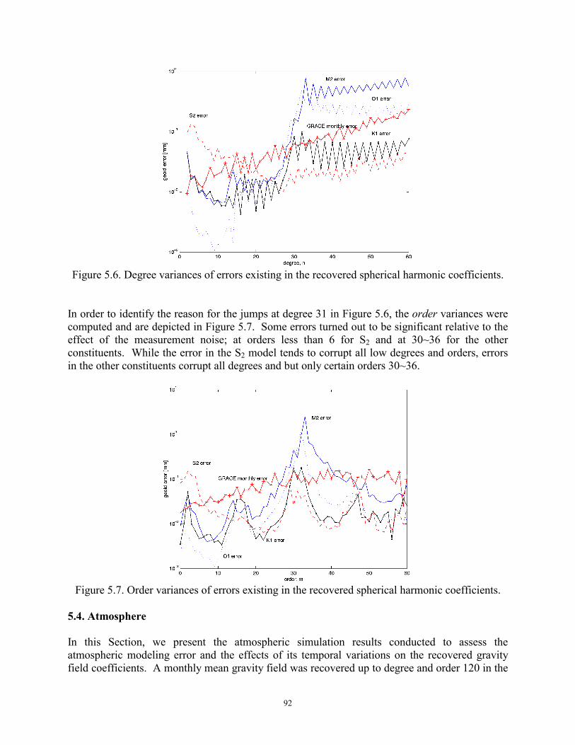
92

Figure 5.6. Degree variances of errors existing in the recovered spherical harmonic coefficients.

In order to identify the reason for the jumps at degree 31 in Figure 5.6, the order variances were computed and are depicted in Figure 5.7. Some errors turned out to be significant relative to the effect of the measurement noise; at orders less than 6 for S2 and at 30~36 for the other constituents. While the error in the S2 model tends to corrupt all low degrees and orders, errors in the other constituents corrupt all degrees and but only certain orders 30~36.

Figure 5.7. Order variances of errors existing in the recovered spherical harmonic coefficients.

5.4. Atmosphere In this Section, we present the atmospheric simulation results conducted to assess the atmospheric modeling error and the effects of its temporal variations on the recovered gravity field coefficients. A monthly mean gravity field was recovered up to degree and order 120 in the

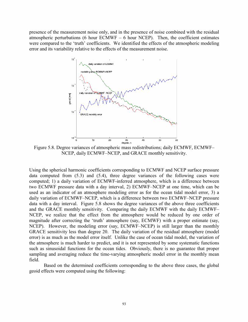
93

presence of the measurement noise only, and in the presence of noise combined with the residual atmospheric perturbations (6 hour ECMWF – 6 hour NCEP). Then, the coefficient estimates were compared to the ‘truth’ coefficients. We identified the effects of the atmospheric modeling error and its variability relative to the effects of the measurement noise.

Figure 5.8. Degree variances of atmospheric mass redistributions; daily ECMWF, ECMWF–

NCEP, daily ECMWF–NCEP, and GRACE monthly sensitivity. Using the spherical harmonic coefficients corresponding to ECMWF and NCEP surface pressure data computed from (5.3) and (5.4), three degree variances of the following cases were computed; 1) a daily variation of ECMWF-inferred atmosphere, which is a difference between two ECMWF pressure data with a day interval, 2) ECMWF–NCEP at one time, which can be used as an indicator of an atmosphere modeling error as for the ocean tidal model error, 3) a daily variation of ECMWF–NCEP, which is a difference between two ECMWF–NCEP pressure data with a day interval. Figure 5.8 shows the degree variances of the above three coefficients and the GRACE monthly sensitivity. Comparing the daily ECMWF with the daily ECMWF–NCEP, we realize that the effect from the atmosphere would be reduced by one order of magnitude after correcting the ‘truth’ atmosphere (say, ECMWF) with a proper estimate (say, NCEP). However, the modeling error (say, ECMWF–NCEP) is still larger than the monthly GRACE sensitivity less than degree 20. The daily variation of the residual atmosphere (model error) is as much as the model error itself. Unlike the case of ocean tidal model, the variation of the atmosphere is much harder to predict, and it is not represented by some systematic functions such as sinusoidal functions for the ocean tides. Obviously, there is no guarantee that proper sampling and averaging reduce the time-varying atmospheric model error in the monthly mean field. Based on the determined coefficients corresponding to the above three cases, the global geoid effects were computed using the following:

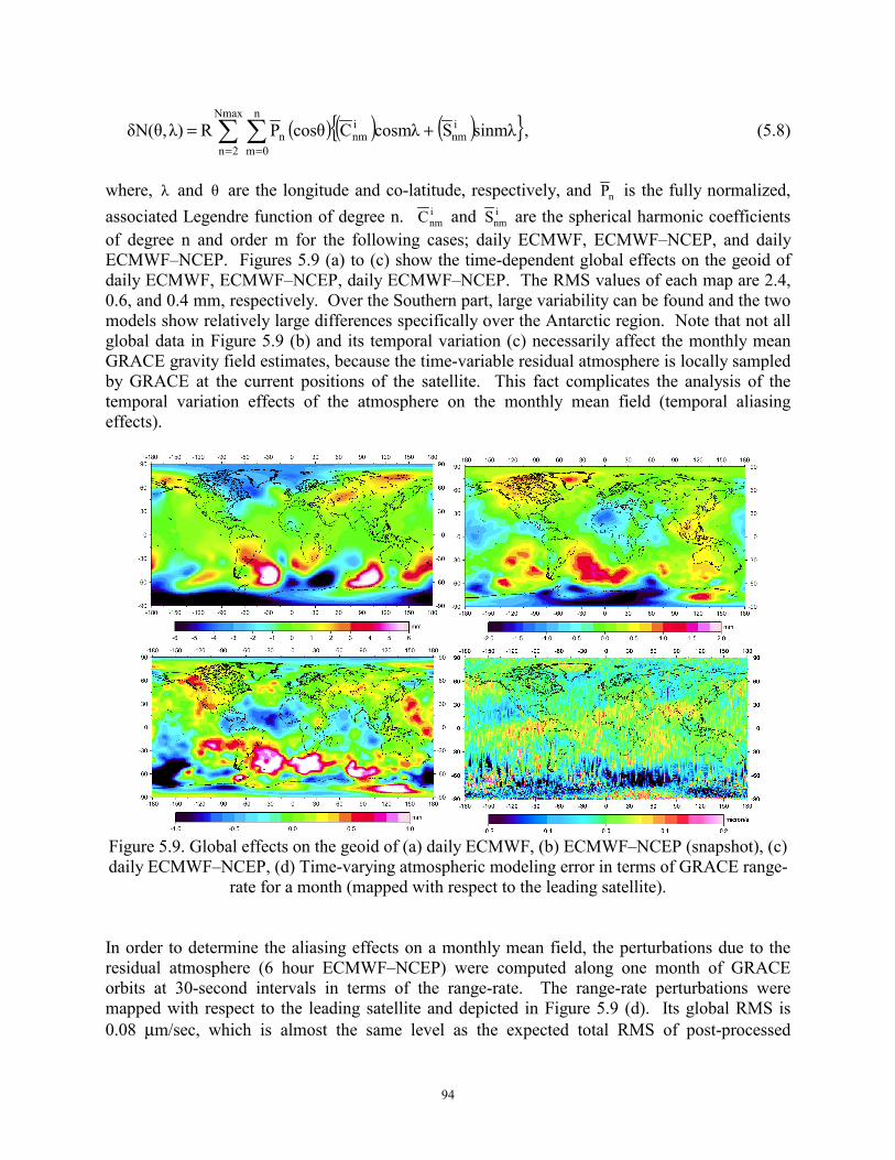
94

( ) ( ) ( ){ }sinmλScosmλCcosθPRλ)δN(θ, inm

inm

Nmax

2n

n

0mn += ∑ ∑

= =, (5.8)

where, λ and θ are the longitude and co-latitude, respectively, and nP is the fully normalized, associated Legendre function of degree n. i

nmC and inmS are the spherical harmonic coefficients

of degree n and order m for the following cases; daily ECMWF, ECMWF–NCEP, and daily ECMWF–NCEP. Figures 5.9 (a) to (c) show the time-dependent global effects on the geoid of daily ECMWF, ECMWF–NCEP, daily ECMWF–NCEP. The RMS values of each map are 2.4, 0.6, and 0.4 mm, respectively. Over the Southern part, large variability can be found and the two models show relatively large differences specifically over the Antarctic region. Note that not all global data in Figure 5.9 (b) and its temporal variation (c) necessarily affect the monthly mean GRACE gravity field estimates, because the time-variable residual atmosphere is locally sampled by GRACE at the current positions of the satellite. This fact complicates the analysis of the temporal variation effects of the atmosphere on the monthly mean field (temporal aliasing effects).

Figure 5.9. Global effects on the geoid of (a) daily ECMWF, (b) ECMWF–NCEP (snapshot), (c) daily ECMWF–NCEP, (d) Time-varying atmospheric modeling error in terms of GRACE range-

rate for a month (mapped with respect to the leading satellite). In order to determine the aliasing effects on a monthly mean field, the perturbations due to the residual atmosphere (6 hour ECMWF–NCEP) were computed along one month of GRACE orbits at 30-second intervals in terms of the range-rate. The range-rate perturbations were mapped with respect to the leading satellite and depicted in Figure 5.9 (d). Its global RMS is 0.08 µm/sec, which is almost the same level as the expected total RMS of post-processed

95

GRACE instrument precision (10 µm in range and 0.1 µm/sec, J.R. Kim in CSR, personal communication, 2002). In this map, notice that the global low degree and order features remain as in the case of perturbations due to the S2 tidal error for a month. In addition, high degree and order features are found because of GRACE’s orbital sampling of the time-variable residual atmosphere.

In the presence of noise and residual atmosphere, monthly data were inverted and the spherical harmonic coefficients were computed up to degree and order 120. For the comparison, the same simulation was done in the presence of noise only. Figures 5.10 (a) and (b) show degree variances and order variances of coefficients errors in both cases of noise only and noise with residual atmospheric perturbation. The monthly global mean of ECMWF and NCEP surface pressure data were computed and the corresponding spherical harmonic coefficients were calculated. The degree variances of coefficient differences between monthly mean ECMWF and NCEP were computed and presented in Figure 5.10 (a). From Figure 5.10 (a), we see two distinct characteristics near the boundary of degree 20~30. The coefficient errors less than degree 20 (in the presence of noise with the residual atmosphere) show a trend and magnitude similar to the monthly global mean ECMWF–NCEP. If the residual atmosphere does not vary in time and is fixed as its global mean for a month, then the error curve of the recovered coefficients from GRACE monthly data would be similar to the sum of the two curves of monthly global mean ECMWF–NCEP and monthly GRACE sensitivity (noise only). However, the realistic (time-variable residual atmosphere) error curve shows significant deviations beyond degree 30 from the noise-only error curve. Therefore, we can conclude that these realistic larger errors over higher degrees (n>30) are due to sampling of time-varying residual atmosphere with a temporal resolution of one month.

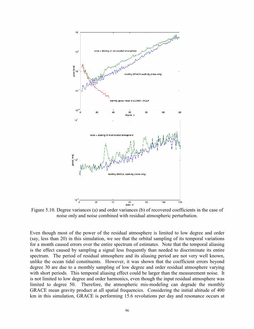
96

Figure 5.10. Degree variances (a) and order variances (b) of recovered coefficients in the case of

noise only and noise combined with residual atmospheric perturbation. Even though most of the power of the residual atmosphere is limited to low degree and order (say, less than 20) in this simulation, we see that the orbital sampling of its temporal variations for a month caused errors over the entire spectrum of estimates. Note that the temporal aliasing is the effect caused by sampling a signal less frequently than needed to discriminate its entire spectrum. The period of residual atmosphere and its aliasing period are not very well known, unlike the ocean tidal constituents. However, it was shown that the coefficient errors beyond degree 30 are due to a monthly sampling of low degree and order residual atmosphere varying with short periods. This temporal aliasing effect could be larger than the measurement noise. It is not limited to low degree and order harmonics, even though the input residual atmosphere was limited to degree 50. Therefore, the atmospheric mis-modeling can degrade the monthly GRACE mean gravity product at all spatial frequencies. Considering the initial altitude of 400 km in this simulation, GRACE is performing 15.6 revolutions per day and resonance occurs at

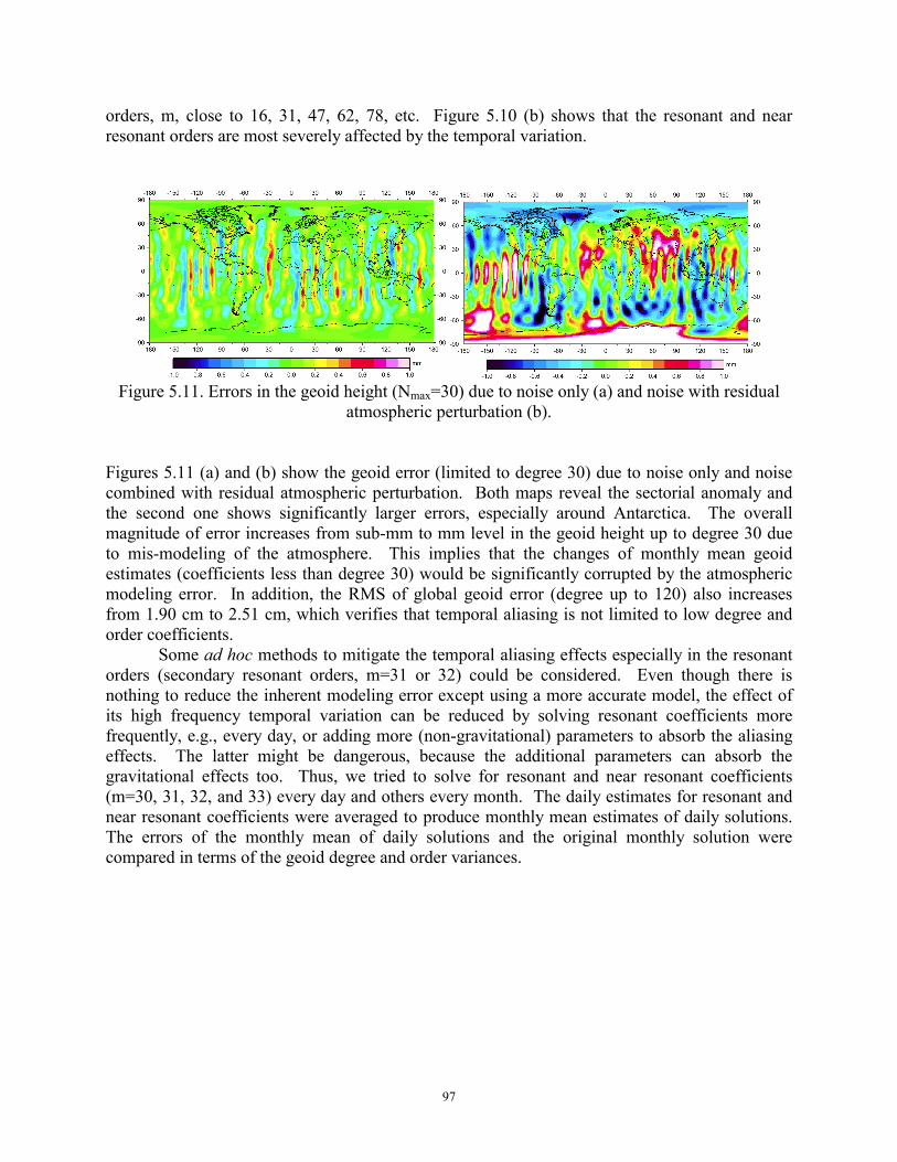
97

orders, m, close to 16, 31, 47, 62, 78, etc. Figure 5.10 (b) shows that the resonant and near resonant orders are most severely affected by the temporal variation.

Figure 5.11. Errors in the geoid height (Nmax=30) due to noise only (a) and noise with residual

atmospheric perturbation (b). Figures 5.11 (a) and (b) show the geoid error (limited to degree 30) due to noise only and noise combined with residual atmospheric perturbation. Both maps reveal the sectorial anomaly and the second one shows significantly larger errors, especially around Antarctica. The overall magnitude of error increases from sub-mm to mm level in the geoid height up to degree 30 due to mis-modeling of the atmosphere. This implies that the changes of monthly mean geoid estimates (coefficients less than degree 30) would be significantly corrupted by the atmospheric modeling error. In addition, the RMS of global geoid error (degree up to 120) also increases from 1.90 cm to 2.51 cm, which verifies that temporal aliasing is not limited to low degree and order coefficients.

Some ad hoc methods to mitigate the temporal aliasing effects especially in the resonant orders (secondary resonant orders, m=31 or 32) could be considered. Even though there is nothing to reduce the inherent modeling error except using a more accurate model, the effect of its high frequency temporal variation can be reduced by solving resonant coefficients more frequently, e.g., every day, or adding more (non-gravitational) parameters to absorb the aliasing effects. The latter might be dangerous, because the additional parameters can absorb the gravitational effects too. Thus, we tried to solve for resonant and near resonant coefficients (m=30, 31, 32, and 33) every day and others every month. The daily estimates for resonant and near resonant coefficients were averaged to produce monthly mean estimates of daily solutions. The errors of the monthly mean of daily solutions and the original monthly solution were compared in terms of the geoid degree and order variances.

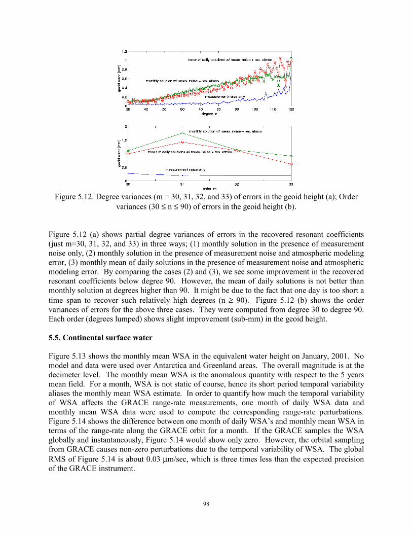
98

Figure 5.12. Degree variances (m = 30, 31, 32, and 33) of errors in the geoid height (a); Order

variances (30 ≤ n ≤ 90) of errors in the geoid height (b). Figure 5.12 (a) shows partial degree variances of errors in the recovered resonant coefficients (just m=30, 31, 32, and 33) in three ways; (1) monthly solution in the presence of measurement noise only, (2) monthly solution in the presence of measurement noise and atmospheric modeling error, (3) monthly mean of daily solutions in the presence of measurement noise and atmospheric modeling error. By comparing the cases (2) and (3), we see some improvement in the recovered resonant coefficients below degree 90. However, the mean of daily solutions is not better than monthly solution at degrees higher than 90. It might be due to the fact that one day is too short a time span to recover such relatively high degrees (n ≥ 90). Figure 5.12 (b) shows the order variances of errors for the above three cases. They were computed from degree 30 to degree 90. Each order (degrees lumped) shows slight improvement (sub-mm) in the geoid height. 5.5. Continental surface water Figure 5.13 shows the monthly mean WSA in the equivalent water height on January, 2001. No model and data were used over Antarctica and Greenland areas. The overall magnitude is at the decimeter level. The monthly mean WSA is the anomalous quantity with respect to the 5 years mean field. For a month, WSA is not static of course, hence its short period temporal variability aliases the monthly mean WSA estimate. In order to quantify how much the temporal variability of WSA affects the GRACE range-rate measurements, one month of daily WSA data and monthly mean WSA data were used to compute the corresponding range-rate perturbations. Figure 5.14 shows the difference between one month of daily WSA’s and monthly mean WSA in terms of the range-rate along the GRACE orbit for a month. If the GRACE samples the WSA globally and instantaneously, Figure 5.14 would show only zero. However, the orbital sampling from GRACE causes non-zero perturbations due to the temporal variability of WSA. The global RMS of Figure 5.14 is about 0.03 µm/sec, which is three times less than the expected precision of the GRACE instrument.

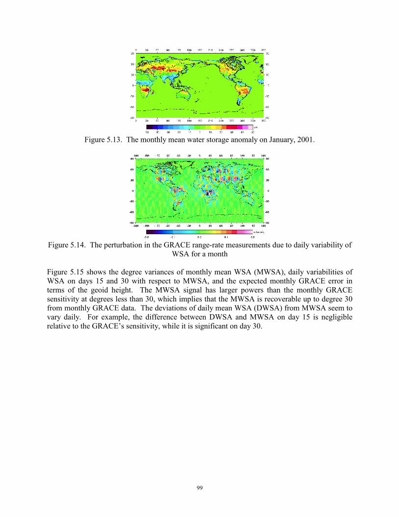
99

Figure 5.13. The monthly mean water storage anomaly on January, 2001.

Figure 5.14. The perturbation in the GRACE range-rate measurements due to daily variability of

WSA for a month Figure 5.15 shows the degree variances of monthly mean WSA (MWSA), daily variabilities of WSA on days 15 and 30 with respect to MWSA, and the expected monthly GRACE error in terms of the geoid height. The MWSA signal has larger powers than the monthly GRACE sensitivity at degrees less than 30, which implies that the MWSA is recoverable up to degree 30 from monthly GRACE data. The deviations of daily mean WSA (DWSA) from MWSA seem to vary daily. For example, the difference between DWSA and MWSA on day 15 is negligible relative to the GRACE’s sensitivity, while it is significant on day 30.

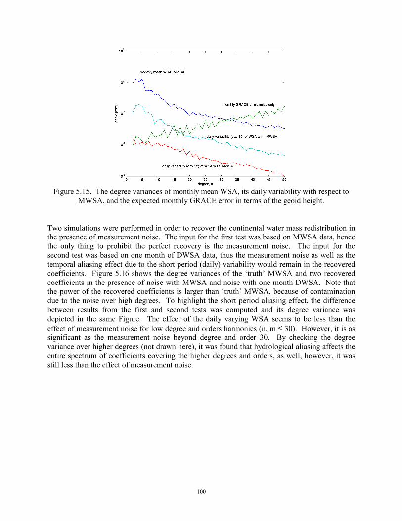
100

Figure 5.15. The degree variances of monthly mean WSA, its daily variability with respect to

MWSA, and the expected monthly GRACE error in terms of the geoid height. Two simulations were performed in order to recover the continental water mass redistribution in the presence of measurement noise. The input for the first test was based on MWSA data, hence the only thing to prohibit the perfect recovery is the measurement noise. The input for the second test was based on one month of DWSA data, thus the measurement noise as well as the temporal aliasing effect due to the short period (daily) variability would remain in the recovered coefficients. Figure 5.16 shows the degree variances of the ‘truth’ MWSA and two recovered coefficients in the presence of noise with MWSA and noise with one month DWSA. Note that the power of the recovered coefficients is larger than ‘truth’ MWSA, because of contamination due to the noise over high degrees. To highlight the short period aliasing effect, the difference between results from the first and second tests was computed and its degree variance was depicted in the same Figure. The effect of the daily varying WSA seems to be less than the effect of measurement noise for low degree and orders harmonics (n, m ≤ 30). However, it is as significant as the measurement noise beyond degree and order 30. By checking the degree variance over higher degrees (not drawn here), it was found that hydrological aliasing affects the entire spectrum of coefficients covering the higher degrees and orders, as well, however, it was still less than the effect of measurement noise.

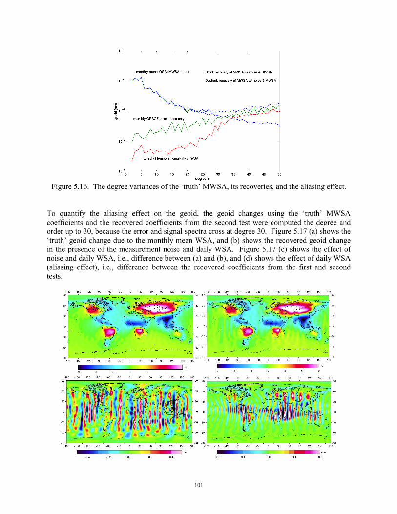
101

Figure 5.16. The degree variances of the ‘truth’ MWSA, its recoveries, and the aliasing effect.

To quantify the aliasing effect on the geoid, the geoid changes using the ‘truth’ MWSA coefficients and the recovered coefficients from the second test were computed the degree and order up to 30, because the error and signal spectra cross at degree 30. Figure 5.17 (a) shows the ‘truth’ geoid change due to the monthly mean WSA, and (b) shows the recovered geoid change in the presence of the measurement noise and daily WSA. Figure 5.17 (c) shows the effect of noise and daily WSA, i.e., difference between (a) and (b), and (d) shows the effect of daily WSA (aliasing effect), i.e., difference between the recovered coefficients from the first and second tests.

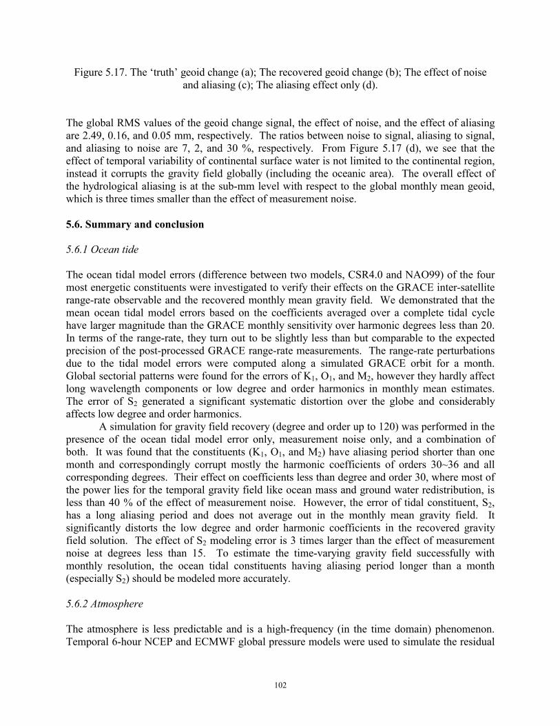
102

Figure 5.17. The ‘truth’ geoid change (a); The recovered geoid change (b); The effect of noise and aliasing (c); The aliasing effect only (d).

The global RMS values of the geoid change signal, the effect of noise, and the effect of aliasing are 2.49, 0.16, and 0.05 mm, respectively. The ratios between noise to signal, aliasing to signal, and aliasing to noise are 7, 2, and 30 %, respectively. From Figure 5.17 (d), we see that the effect of temporal variability of continental surface water is not limited to the continental region, instead it corrupts the gravity field globally (including the oceanic area). The overall effect of the hydrological aliasing is at the sub-mm level with respect to the global monthly mean geoid, which is three times smaller than the effect of measurement noise. 5.6. Summary and conclusion 5.6.1 Ocean tide The ocean tidal model errors (difference between two models, CSR4.0 and NAO99) of the four most energetic constituents were investigated to verify their effects on the GRACE inter-satellite range-rate observable and the recovered monthly mean gravity field. We demonstrated that the mean ocean tidal model errors based on the coefficients averaged over a complete tidal cycle have larger magnitude than the GRACE monthly sensitivity over harmonic degrees less than 20. In terms of the range-rate, they turn out to be slightly less than but comparable to the expected precision of the post-processed GRACE range-rate measurements. The range-rate perturbations due to the tidal model errors were computed along a simulated GRACE orbit for a month. Global sectorial patterns were found for the errors of K1, O1, and M2, however they hardly affect long wavelength components or low degree and order harmonics in monthly mean estimates. The error of S2 generated a significant systematic distortion over the globe and considerably affects low degree and order harmonics.

A simulation for gravity field recovery (degree and order up to 120) was performed in the presence of the ocean tidal model error only, measurement noise only, and a combination of both. It was found that the constituents (K1, O1, and M2) have aliasing period shorter than one month and correspondingly corrupt mostly the harmonic coefficients of orders 30~36 and all corresponding degrees. Their effect on coefficients less than degree and order 30, where most of the power lies for the temporal gravity field like ocean mass and ground water redistribution, is less than 40 % of the effect of measurement noise. However, the error of tidal constituent, S2, has a long aliasing period and does not average out in the monthly mean gravity field. It significantly distorts the low degree and order harmonic coefficients in the recovered gravity field solution. The effect of S2 modeling error is 3 times larger than the effect of measurement noise at degrees less than 15. To estimate the time-varying gravity field successfully with monthly resolution, the ocean tidal constituents having aliasing period longer than a month (especially S2) should be modeled more accurately. 5.6.2 Atmosphere The atmosphere is less predictable and is a high-frequency (in the time domain) phenomenon. Temporal 6-hour NCEP and ECMWF global pressure models were used to simulate the residual

103

atmospheric perturbations on the GRACE orbit for a month. The GRACE simulations were performed in order to recover the gravity coefficients with maximum degree of 120 by fully inverting one month of data in the presence of noise and residual atmosphere, i.e., ECMWF–NCEP 6-hour resolution. We quantified the time-variable effects of atmospheric modeling error in the range-rate observations and analyzed them in the recovered monthly mean gravity coefficients.

The global RMS of ECMWF–NCEP is slightly less than the precision of GRACE range-rate measurements, however it was found that the residual atmosphere can considerably contaminate the monthly mean gravity coefficients over all degrees and orders. The errors in the recovered coefficients less than degree 20 due to the atmospheric mis-modeling are large enough to corrupt the temporal gravity (geoid) estimates significantly. The errors beyond degree 30 have larger magnitude than the measurement noise over all degrees, thus the temporal aliasing effect degrades the overall performance (all degrees) of monthly mean GRACE gravity products. That is, the atmospheric aliasing effect is not limited to low degree and order harmonics. For example, the mean geoid estimates up to maximum degree 120 will have 30 % more error due to the residual atmosphere. By looking at the order variance, it was found that resonant orders (even m = 78) were especially contaminated by the residual atmosphere, even though the input residual atmosphere was limited in degree and order up to 50. As an alternative solution strategy, we demonstrated that a more frequent (e.g., daily) estimation of resonant coefficients could help decrease the effects coming from the temporal variability of the residual atmosphere. The level of atmospheric modeling error might be underestimated in this study, because two models, ECMWF and NCEP, are not completely independent. The real error effect may be larger than shown here, however, the characteristics would remain same. The accuracy of temporal gravity (geoid) estimation (e.g., continental surface water and ocean mass redistribution) clearly is limited by the atmospheric mis-modeling. 5.6.3 Continental surface water Based on NCEP/NCAR daily CDAS-1 data, it was attempted to quantify the effects of the daily variability of the continental water mass on the monthly mean gravity estimates. The range-rate perturbations due to daily variability were computed and its global RMS was about 3 times smaller than the precision of GRACE range-rate measurements. Two distinct simulations were performed to identify the effects of daily variability. The monthly mean continental surface water mass was recovered in two ways: 1) recovery in the presences of monthly mean WSA (no variability in a month) and measurement noise; 2) recovery in the presences of one month of daily mean WSA and measurement noise.

The results showed that the corruption due to the daily variability of hydrology on the recovered harmonic coefficients (less than degree 30) is about one order of magnitude less than the corruption due to the measurement noise. Beyond degree 30, the errors induced by the daily variability are still less than (but, approximately follow) the errors due to the measurement noise. All recovered coefficients were affected by the daily variability, even though the input of the hydrology signal was limited in spatial degree to 50. In terms of the geoid height effects, the overall effect of the daily variability was at the level of sub-mm and it was about 3 times smaller than the effect of measurement noise. Therefore, it can be said that the effects of the high frequency temporal (daily) variability of the continental water mass are smaller than the effects

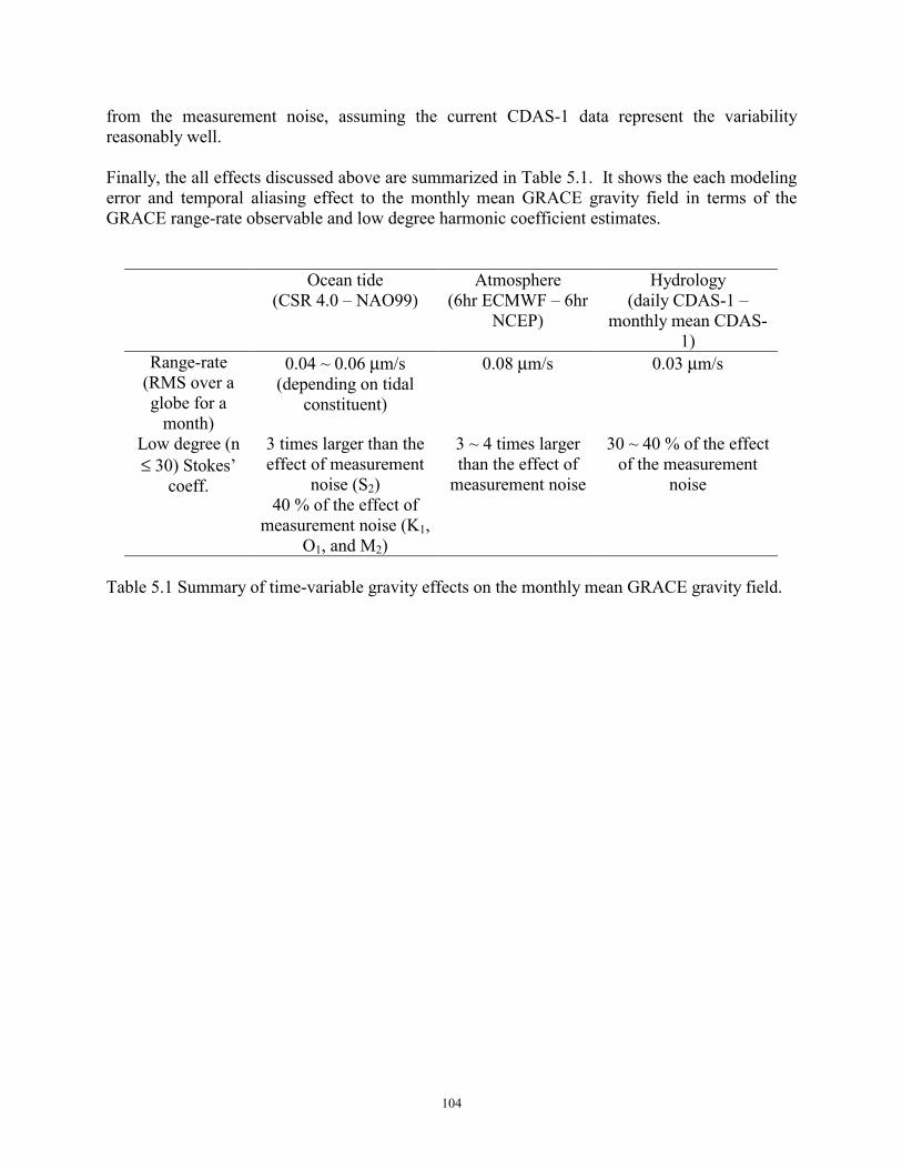
104

from the measurement noise, assuming the current CDAS-1 data represent the variability reasonably well. Finally, the all effects discussed above are summarized in Table 5.1. It shows the each modeling error and temporal aliasing effect to the monthly mean GRACE gravity field in terms of the GRACE range-rate observable and low degree harmonic coefficient estimates.

Ocean tide (CSR 4.0 – NAO99)

Atmosphere (6hr ECMWF – 6hr

NCEP)

Hydrology (daily CDAS-1 –

monthly mean CDAS-1)

Range-rate (RMS over a globe for a

month)

0.04 ~ 0.06 µm/s (depending on tidal

constituent)

0.08 µm/s 0.03 µm/s

Low degree (n ≤ 30) Stokes’

coeff.

3 times larger than the effect of measurement

noise (S2) 40 % of the effect of

measurement noise (K1, O1, and M2)

3 ~ 4 times larger than the effect of

measurement noise

30 ~ 40 % of the effect of the measurement

noise

Table 5.1 Summary of time-variable gravity effects on the monthly mean GRACE gravity field.

105

6. CONCLUSION New observation equations and an efficient inversion method were developed and implemented for determination of the Earth’s global gravity field using satellite measurements. On the basis of the energy conservation principle, in situ (on-orbit) and along track disturbing potential and potential difference observations were computed using data from accelerometer- and GPS receiver-equipped satellites, such as CHAMP and GRACE. The efficient iterative inversion method provided the exact estimates as well as an approximate, but very accurate error variance-covariance matrix of the least squares system for both satellite missions. The global disturbing potential observations were then used to determine a gravity field solution (OSU02A, Nmax=50, 16 days of CHAMP data). An evaluation of the model using independent GPS/leveling derived geoid and Arctic gravity anomaly data, and comparisons with existing gravity models, EGM96 and GRIM5C1, and new models, EIGEN1S and TEG4 which include CHAMP data, indicate that OSU02A is commensurate in geoid accuracy and, like other new models, it yields some improvement (10% better fit) in the polar region at wavelengths longer than 800 km. The significant accelerometer calibration and (possible) empirical force parameters were estimated prior to the gravity estimation. The gravity solutions based on 10 days of dynamic, reduced-dynamic, and kinematic orbits were determined, and it was found that although the solutions based on dynamic orbits are substantially more accurate than others, more correlation with the a priori gravity field was found. The approximate covariance matrix based on a pre-conditioner turned out to be extremely efficient in computational time and to be reasonably accurate to provide practically the same results as the true covariance matrix. For the first time, the temporal gravity field from CHAMP was presented. Considering the formal monthly error of CHAMP monthly mean solutions, only low degree harmonic coefficients (degree 2 and 3) were computed for secular, annual, and semi-annual variations of the Earth’s gravity field. The annual components were compared with the currently available solutions from SLR, showing correlation of 60~80% with one solution. An annual geoid change at the level of 1 mm would be expected. Using simulated potential difference observations expected from the GRACE mission, the gravity field coefficients and approximate error covariance up to degree and order 120 were estimated using minimal computer memory and relatively short computational time. Based on the monthly GRACE noise-only simulation, the geoid was obtained with an accuracy of a few cm and with a resolution (half wavelength) of 160 km. However, the geoid accuracy can become worse by a factor of 6~7 because of spatial aliasing. The approximate error covariance was found to be a very good accuracy measure of the estimated coefficients, geoid, and gravity anomaly. The temporal gravity field, representing the monthly mean continental water mass redistribution, was recovered in the presence of measurement noise and high frequency (daily) temporal variation. The resulting recovered temporal gravity fields have about 0.2 mm errors in terms of geoid height with a resolution of 670 km. For the time series of monthly mean (static) GRACE gravity fields, the known temporal effects due to ocean tides and atmospheric mass redistribution should be removed from GRACE measurements using the most accurate models/data. The effects due to the inherent modeling errors and temporal aliasing caused by ocean tides, atmosphere, and ground surface water mass on monthly mean GRACE gravity estimates were quantified. The results are based on simulations of GRACE range-rate perturbations due to modeling error along the orbit and a full inversion of GRACE data. For ocean tides, the study based on the model difference, CSR4.0–

106

NAO99, indicated that some residual constituents like in S2 may cause errors 3 times larger than the measurements noise at harmonic degrees less than 15 in the monthly mean estimates. On the other hand, residual constituents in K1, O1, and M2 were reduced by monthly averaging below the measurement noise level. For the atmosphere, the difference in models, ECMWF–NCEP, produced errors in GRACE range-rate measurements as strong as the measurement noise. They corrupted all recovered coefficients and introduce 30 % more error in the global monthly geoid estimates up to maximum degree 120. However, the analysis based on daily CDAS-1 data for continental surface water mass redistribution indicated that the daily soil moisture and snow depth variations affect the monthly mean GRACE recovery less than the measurement noise. Even though there are countless number of unsolved and remaining problems/applications for satellite gravimetry, the following studies would be suggested as important further investigations: 1) As the CHAMP mission progresses, we should incorporate more years of CHAMP data to obtain more robust time-variable gravity field solutions and resolve the unknown reason for very poor solutions of C22, S22, and C30 coefficients. 2) Parallel processing of the iterative inversion on a cluster platform will reduce even more significantly the computational time. 3) The combination of CHAMP/GRACE solutions and surface data (or a combination model like EGM96) with weighting based on the approximate error covariance should be investigated. 4) Some better methods to reduce the temporal as well as spatial aliasing effects, occurring significantly (near) resonant orders and near Nyquist degrees, respectively, would be developed. 5) The local use of in situ potential (difference) measurements should be considered to recover the local phenomena like continental water mass redistribution and enhance the spatial resolution over the polar region. A direct downward continuation of the point measurement and the use of local basis functions such as spherical cap harmonics, Slepians, and spherical harmonic wavelets should be studied. 6) The quite complete coverage of CHAMP and GRACE satellites provides significantly enhanced gravity information over the polar region. New geophysical and geodynamical interpretation over the polar region should be done with the CHAMP/GRACE data. The use of long wavelength satellite gravity information would constrain or correct the possible error of high resolution Arctic gravity data, which were inconsistently obtained from diverse methods and many agencies in area-by-area.

107

REFERENCES Albertella, A., Migliaccio, F., and Sanso, F.: The Aliasing Effect in Coefficients Estimation, IAG

Symposia, 106, R. Rapp and F. Sanso (Eds.), 10-15, Springer-Verlag, Berlin, 1990. Arfken, G. B. and H. J. Weber: Mathematical methods for physicists. Academic Press, 1995. Bettadpur, S., and M. Watkins: GRACE gravity science & its impact on mission design, Spring

AGU, 2000. CDDISA, http://cddisa.gsfc.nasa.gov/igsdc/, 2002 Chao, B. F., and A. Y. Au: Temporal variation of the Earth’s low-degree zonal gravitational field

caused by atmosphereic mass redistribution: 1980-1988, J. Geophys. Res., 96 (B4), 6569-6575, 1991.

Cheng, M. K., Gunter, B., Ries, J., Chambers, D. P., and Tapley, B. D.: Temporal variations in the earth’s gravity field from SLR and CHAMP GPS data. In I. N. Tziavos (Ed.), Gravity and Geoid 2002 (pp. 424–431), 3 rd meeting of the IGGC, Thessaloniki, Greece, 2003.

Colombo, O.: Numerical methods for harmonic analysis on the sphere, Report No. 310, Dept. Geod. Sci. and Surv., Ohio State Univ., Columbus, Ohio, 1981.

Davis, E., Dunn, C., Stanton, R., and Thomas, J.: The GRACE mission: meeting the technical challenges, 50th International Astronautical Congress, October 4-8, 1999.

Ditmar, P. and Klees, R.: A method to compute the Earth’s gravity field from SGG/SST data to be acquired by the GOCE satellite, Delft University Press, 2002.

Eanes, R.: A study of temporal variations in Earth’s gravitational field using Lageos-1 laser ranging observations, Ph.D. dissertation, Univ. of Texas as Austin, 1995.

Eanes, R. and Bettadpur, S., The CSR 3.0 global ocean tide model, CSR-TM-95-06, Center for Space Research, Technical memorandum, December, 1995.

Gerlach, C., Sneeuw, N., Visser, P., and Švehla, D.:, CHAMP gravity field recovery with the energy balance approach: first results, Proc. First CHAMP International Science Meeting, 2002.

GGFC: 2002, The IERS Global Geophysical Fluids Center, Special Bureau for Hydrology, http://www.csr.utexas.edu/research/ggfc.

Golub, G., and van Loan, C.: Matrix computations, The Johns Hopkins University Press, 1996. GRACE Science Mission Requirement Document: 2000, GRACE 327-720, June, 2000. Gruber, T., A. Bode, Ch. Reigber, P. Schwintzer, G. Balmino, R. Biancale, and J.-M. Lemoine,

GRIM5-C1: Combination solution of the global gravity field to degree and order 120, Geophys. Res. Lett., 27, 4005-4008, 2000.

Han, D., and Wahr, J.: The viscoelastic relaxation of a realistically stratified Earth, and a further analysis of post glacial rebound, Geopy. J. Int., 120, 287-311, 1995.

Han, S.-C., Jekeli, C., and Shum, C.K.: Efficient gravity field recovery using in situ disturbing potential observables from CHAMP, Geophy. Res. Letters, 29(16), 10.1029/2002GL015180, 2002a.

Han, S.-C., Jekeli, C., Shum, C.K.: Aliasing and Polar Gap Effect on Geopotential Coefficient Estimation: Space-wise Simulation Study of GOCE and GRACE, IAG Geodesy Symposia, 125, J. Adam and K.-P. Schwarz (Eds), 181-186, Springer-Verlag, Berlin, 2002b.

Han, S.-C., Jekeli, C., Shum, C.K.: Static and Temporal Gravity Field Recovery Using GRACE Potential Difference Observables, Advances in Geosciences, Vol.1, No.1, pp.19-26, 2003.

Heiskanen, W. and Moritz, H.: Physical Geodesy, Freeman, San Francisco, 1967.

108

Howe E. and Tscherning C.: Preliminary analysis of CHAMP state vector and accelerometer data for the recovery of the gravity potential, 1st CHAMP Science Meeting, Potsdam, Germany, Jan. 22-25, 2002.

Hwang, C.: Gravity recovery using COSMIC GPS data: application of orbital perturbation theory, J. Geodesy, 75, 117-136, 2001.

Jekeli, C.: Spherical harmonic analysis, aliasing, and filtering, J. Geodesy, 70, 214-223, 1996. Jekeli, C.: The determination of gravitational potential differences from satellite-to-satellite

tracking, Celestial Mechanics and Dynamical Astronomy, 75, 85-101, 1999. Jekeli, C. and Rapp, R.: Accuracy of the determination of mean anomalies and mean geoid

undulations from a satellite gravity mapping mission, Report No. 307, Dept. of Geod. Sci., Ohio State University, Columbus, 1980.

Jekeli, C., and Garcia, R.: Local geoid determination with in situ geopotential data obtained from satellite-to-satellite tracking, IAG Symposium Series, 123, M.G. Sideris (Ed.), 123-128, Springer-Verlag, Berlin, 2001.

Kalnay, E., et al., The NCEP/NCAR 40-Year Reanalysis Project, Bull. Am. Met. Soc., 77, 437-471, 1996.

Kenyon, S., and R. Forsberg, Arctic Gravity Project - a status, in Gravity, Geoid and Geodynamics 2000, International Association of Geodesy Symposia, vol. 123, edited by M. Sideris, 391-395, Springer-Verlag, 2001.

Kim, J.R., et al., Simulations of the Gravity Recovery and Climate Experiment (GRACE) Mission, AAS/AIAA Space Flight Mechanics Meeting, AAS 99-144, Breckenridge, Colorado, Feburuary 7-10, 1999.

Kim, J., Roesset, P., Bettadpur, S., Tapley, B., and Watkins, M.: Error analysis of the Gravity Recovery and Climate Experiment (GRACE), IAG Symposium Series, 123, M. Sideris (eds), 103-108, Springer-Verlag, Berlin, 2001.

Klees, R., Koop, R., Visser, P., van den IJssel, J., and Rummel, R.: Data analysis for the GOCE mission, IAG Symposium Series, 121, K. Schwarz (ed), 68-74, Springer-Verlag, Berlin, 2000a.

Klees R., Koop, R., Visser, P., and van den IJssel, J.: Efficient gravity field recovery from GOCE gravity gradient observations, J. Geodesy, 74, 561-571, 2000b.

Knudsen, P., and O. Andersen, Correcting GRACE gravity fields for ocean tide effects, in press, Geophys. Res. Let., 2002.

Kusche, J.: On fast Multigrid Iteration Techniques for the Solution of Normal Equations in Satellite Gravity Recovery, Journal of Geodynamics 33:173-186, 2002

Lemoine, F., S. Kenyon, J. Factor, R. Trimmer, N. Pavlis, D. Chinn, C. Cox, S. Klosko, S. Luthcke, M. Torrence, Y. Wang, R. Williamson, E. Pavlis, R. Rapp, and T. Olson: The development of the joint NASA GSFC and the National Imagery and Mapping Agency (NIMA) geopotential model EGM96, NASA Technical Paper NASA/TP-1998-206861, Goddard Space Flight Center, Greenbelt, 1998.

Matsumoto, K., Takanezawa, T., and Ooe, M., Ocean tide models developed by assimilating Topex/Poseidon altimeter data into hydronynamical model: a global model and a regional model around Japan, Journal of Oceanography, Vol. 56, pp. 567-581, 2000.

McCarthy, D., IERS Conventions (1996), IERS Technical Note, 1996. McCarthy, D., IERS Conventions (2000), IERS Technical Note, 2000. Moritz, H.: Geodetic Reference System 1980. Bull. Geod., 66(2), 187-192, 1992.

109

Nerem, S., Wahr, J., and Leuliette, E.: Measuring the distribution of ocean mass using GRACE, Space Sci. Rev., in review, 2002.

Nerem, R.S., R.J. Eanes, P. F. Thompson, and J.L. Chen, Observations of annual variations of the Earth's gravitational field using satellite laser ranging and geophysical models, Geophy. Res. Ltr., 27, 1783-1786, 2000.

Pail, R., and Plank, G.: Assessment of three numerical solution strategies for gravity field recovery from GOCE satellite gravity gradiometry implemented on a parallel platform, J. Geodesy, 76, 462-474, 2002.

Parke, M. E., R. H. Stewart, D.L. Farless, and D. E., Cartwright, On the Choice of Orbits for an Altimetric Satellite to Study Ocean Circulation and Tides, J. Geophys. Res., 92, 11693-11707, 1987.

Pavlis, N.: Modeling and Estimation of a Low Degree Geopotential Model From Terrestrial Gravity Data, Report No. 386, Dept. of Geod. Sci., Ohio State University, Columbus, 1988.

Perret, A., Biancale, R., Camus, A., Lemoine, J., Fayard, T., Loyer, S., Perosanz, F., and Sarrailh, M.: 2001, ‘CHAMP mission: STAR commissioning phase calibration/validation activities by CNES’, Vol. 1&2, CNES, May 2001, Toulouse.

O’Keefe, J. A.: An application of Jacobi’s integral to the motion of an earth satellite, Astron. J. 62(8), 266–267, 1957.

Ray, R. D., R. J. Eanes, G. D. Egbert, N. K. Pavlis: Error spectrum for the global M2 ocean tide, Geophys. Res. Lett. 28, 21–24, 2001.

Reigber, Ch.: Gravity recovery from satellite tracking data. In: Sanso F., and Rummel R. (eds), Theory of satellite geodesy and gravity field determination, Lecture notes in Earth sciences, vol. 25, Springer, Berlin Heidelberg New York, pp.197-234, 1989.

Reigber, C., Kang, Z., König, R., and Schwintzer, P.: CHAMP, A minisatellite mission for geopotential and atmospheric research’, Spring AGU Meeting, May 1996, Baltimore, 1996.

Reigber, Ch., G. Balmino, P. Schwintzer, R. Biancale, A. Bode, J.-M. Lemoine, R. König, S. Loyer, K.-H. Neumayer, J.-C. Marty, F. Barthelmes, F. Perosanz, and S.Y. Zhu: A high-quality global gravity field model from CHAMP GPS tracking data and accelerometry (EIGEN-1S), Geophys. Res. Lett., 29 (14), 10.1029/2002GL015064 2002.

Rim H., Kang K., Nagel P., Yoon S., Bettadpur S., B. Schutz B., Tapley B., CHAMP Precision Orbit Determination, AAS/AIAA 2001, Paper No. AAS-01-334, 2001.

Rodell, M., and J.S. Famiglietti, Detectibility of Variations in Continental Water Storage from Satellite Observations of the Time-variable Gravity Field, Wat. Resour. Res., 35 (9), 2705-2723, 1999.

Rosborogh G.W., Tapley B.D.: Radial, transverse, and normal satellite position perturbations due to the geopotential, Cel. Mech., 40, 409-421, 1987.

Rowlands, D., Ray, R., Chinn, D., and Lemoine, F.: Short-arc analysis of intersatellite tracking data in a gravity mapping mission, J. Geodesy, 76, 307-316, 2002.

Rummel, R.: Geoid heights, geoid height differences, and mean gravity anomalies from low-low satellite-to-satellite tracking – an error analysis, Report No. 306, Dept. of Geod. Sci., Ohio State University, Columbus, 1980.

Rummel et al.: Gravity Field and Steady-State Ocean Circulation Mission, Earth Explorer Mission Selection Workshop Report, SP-1233(1), European Space Agency, Granada, Spain, 1999.

Schuh, W.-D.: Tailored numerical solution strategies for the global determinations of the Earth’s gravity field, Mitteilungen d. Geodat. Inst. d. TU Graz, no. 81, Graz, 1996.

110

Schuh, W.-D., Sünkel, H., Hausleitner, W., and Hoke, E.: Refinement of iterative procedures for the reduction of spaceborne gravimetry data, ESA-Project CIGAR IV, WP4, Final Report, ESA contract 152163, ESTEC/JP/95-4-137/MS/nr, European Space Agency, Noordwijk, pp.157-212, 1996.

Shum ,C.K., Han, S.-C., Jekeli, C., Yi, Y., Zhao, C., Dumrongchai, P., Kenyon, S., Roman, D., Zhang, K., Lu, Y., and Zhu, Y.: Accuracy Assessment of Current Gravity Field Models, paper presented at International Association of Geodesy Symposia, Budapest, Hungary, 2001.

Sneeuw, N.: A semi-analytical approach to gravity field analysis from satellite observations, Deutsche Geod¨ atische Kommission, Reihe C, No. 527, 2000.

Sneeuw, N., Gerlach, C., Švehla, D., and Gruber, C.: A first attempt at time-variable gravity recovery from CHAMP using the energy balance approach, The third meeting of the international gravity and geoid commission, August 2002, Thessaloniki, Greece.

Sünkel, H. (ed.): From Eötvös to Milligal, ESA Final Report, ESA/ESTEC, contract no.13392/98/NL/GD, Graz, Austria, 2000.

Tapley, B., Reigber, C., and Melbourne, W.: Gravity Recovery And Climate Experiment (GRACE) mission’, Spring AGU Meeting, May 1996, Baltimore.

Tapley, B., S. Bettadpur, D. Chambers, M. Cheng, K. Choi, B. Gunter, Z. Kang, J. Kim, P. Nagel, J. Ries, H. Rim, P. Roesset, and I. Roundhill, Gravity field determination from CHAMP using GPS tracking and accelerometer data: initial results, paper presented at the first CHAMP Science Meeting, Potsdam, Germany, 2002.

Thomas, J.: An analysis of gravity field estimation based on intersatellite dual one-way biased ranging, JPL Publication 98-15, 3-13, 1999.

Tscherning, C., Rapp, R., and Goad, C.: A Comparison of Methods for computing Gravimetric Quantities from High Degree Spherical Harmonic Expansions, Manuscripta Geodaetica, 8, 249-272, 1983.

Velicogna, I., J. Wahr, and H. van den Dool, Can surface pressure be used to remove atmospheric contributions from GRACE data with sufficient accuracy to recover hydrological signals?, J. Geophys. Res., 106 (B8), 16415-16434, 2001.

Visser, P., Sneeuw, N., and Gerlach, C.: Energy integral method for gravity field determination from satellite orbit coordinates, J. Geodesy, submitted, 2002.

Wagner, C.: Direct determination of gravitational harmonics from low-low GRAVSAT data, J. Geophy. Res., 88(B12), 10309-10321, 1983.

Wahr, J., Molenaar, M., and Bryan, F.: Time variability of the Earth’s gravity field: hydrological and oceanic effects and their possible detection using GRACE, J. Geophy. Res., 103, 30205-30229, 1998.

Wahr, J., and Velicogna, I.: What might GRACE contribute to studies of post glacial rebound?, Space Sci. Rev., in review, 2002.

Wolff, M.: Direct determination of gravitational harmonics from low-low GRAVSAT data, J. Geophy. Res., 88, 10309-10321, 1969.