Efficient Diversification

CHAPTER 6

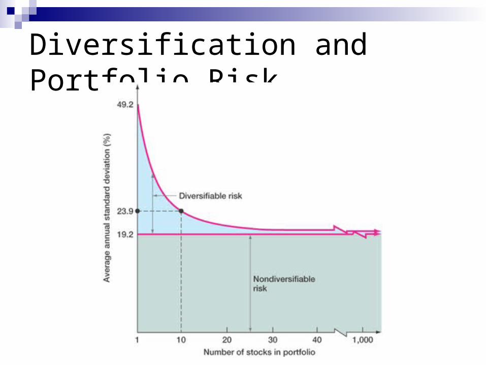
Diversification and Portfolio Risk

Suppose your portfolio has only 1 stock, how many sources of risk can affect your portfolio? Uncertainty at the market level Uncertainty at the firm level

Market risk Systematic or Nondiversifiable

Firm-specific risk Diversifiable or nonsystematic

If your portfolio is not diversified, the total risk of portfolio will have both market risk and specific risk

If it is diversified, the total risk has only market risk

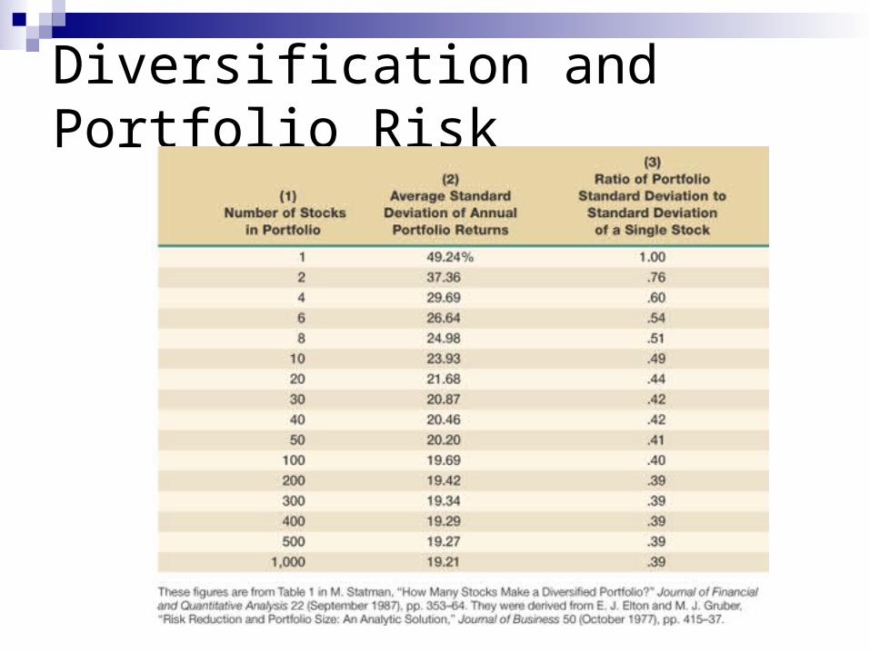
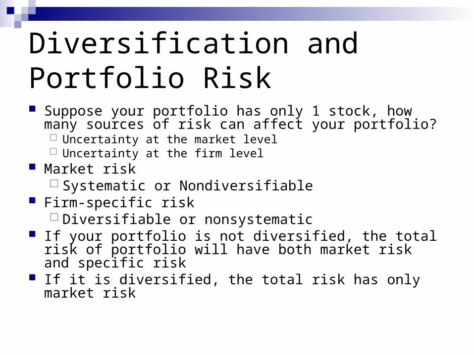
Diversification and Portfolio Risk

Diversification and Portfolio Risk

Figure 6.1 Portfolio Risk as a Function of the Number of Stocks

Covariance and Correlation

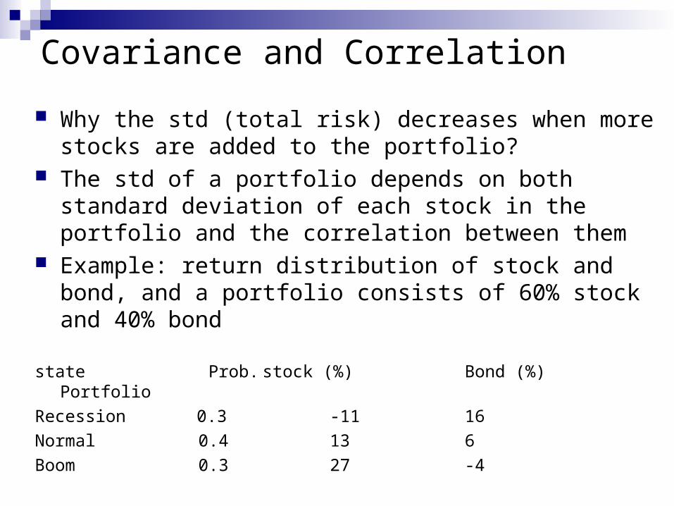
Why the std (total risk) decreases when more stocks are added to the portfolio?

The std of a portfolio depends on both standard deviation of each stock in the portfolio and the correlation between them

Example: return distribution of stock and bond, and a portfolio consists of 60% stock and 40% bond

state Prob. stock (%) Bond (%) Portfolio

Recession 0.3 -11 16

Normal 0.4 13 6

Boom 0.3 27 -4

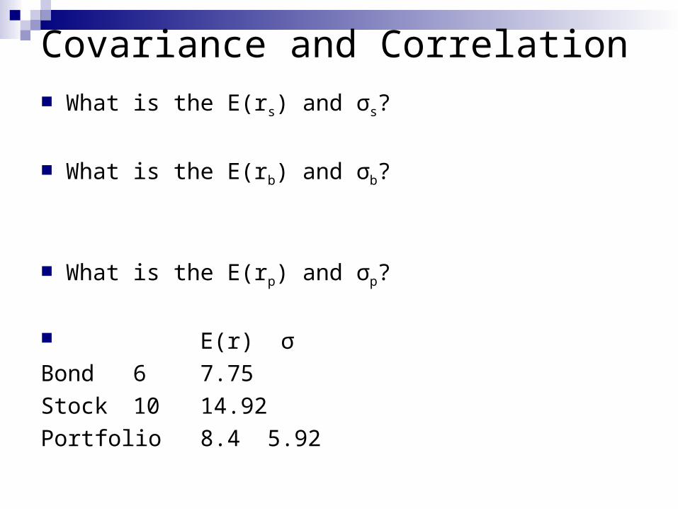
Covariance and Correlation What is the E(rs) and σs?

What is the E(rb) and σb?

What is the E(rp) and σp?

E(r) σ

Bond 6 7.75

Stock 10 14.92

Portfolio 8.4 5.92

Covariance and Correlation When combining the stocks into the portfolio, you get the average

return but the std is less than the average of the std of the 2 stocks in the portfolio

Why? The risk of a portfolio also depends on the correlation between 2 stocks How to measure the correlation between the 2 stocks Covariance and correlation

bs

bsbs

bb

n

issibs

rrCovrrCorr

rEirrEirprrCov

),(

),(

)()()()(),(1

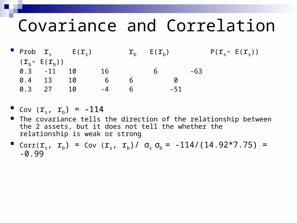
Covariance and Correlation Prob rs E(rs) rb E(rb) P(rs- E(rs))(rb-

E(rb))

0.3 -11 10 16 6 -630.4 13 10 6 6 00.3 27 10 -4 6 -51

Cov (rs, rb) = -114-114 The covariance tells the direction of the relationship between the 2 assets, but

it does not tell the whether the relationship is weak or strong Corr(rs, rb) = Cov (rs, rb)/ σs σb = -114/(14.92*7.75) = -0.99

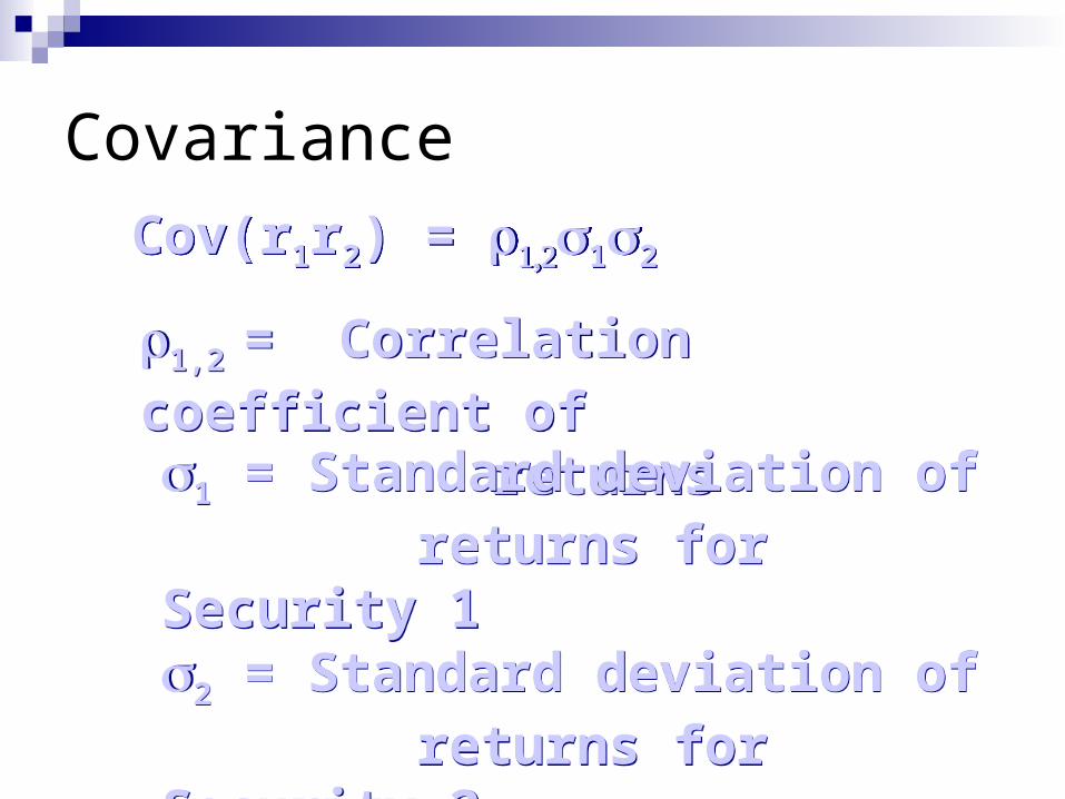
Covariance

1,2 = Correlation coefficient of returns

1,2 = Correlation coefficient of returns

Cov(r1r2) = 12Cov(r1r2) = 12

1 = Standard deviation of returns for Security 12 = Standard deviation of returns for Security 2

1 = Standard deviation of returns for Security 12 = Standard deviation of returns for Security 2

Correlation Coefficients: Possible Values

If If = 1.0, the securities would be = 1.0, the securities would be perfectly positively correlatedperfectly positively correlated

If If = - 1.0, the securities would be = - 1.0, the securities would be perfectly negatively correlatedperfectly negatively correlated

If If ρρ = 0, no correlation = 0, no correlation

Range of values for 1,2

-1.0 < < 1.0

Two Asset Portfolio St Dev – Stock and Bond

Deviation Standard Portfolio

Variance Portfolio

)()()(

2

2

,

22222 2

p

p

SBBSSBSSBBp

ssBBp

ssBBp

wwww

rEwrEwrE

rwrwr

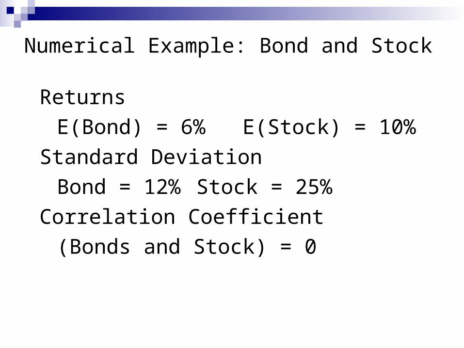
Numerical Example: Bond and Stock

Returns

E(Bond) = 6% E(Stock) = 10%

Standard Deviation

Bond = 12% Stock = 25%

Correlation Coefficient

(Bonds and Stock) = 0

Numerical Example: Bond and Stock

Case 1: Weights Bond = .5 Stock = .5

What is the E(rp) and σp

E(rp) = 8%

σp = 13.87%

Average std = (25+12)/2 = 18.5 By combining stocks, get average return, but the risk is lower

than average

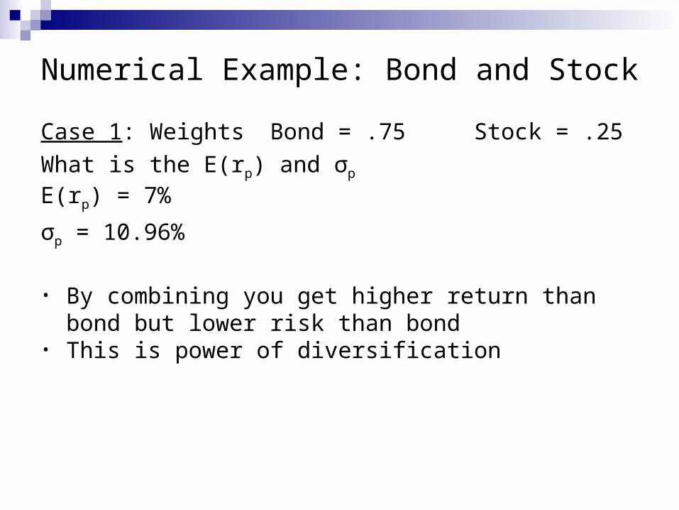
Numerical Example: Bond and Stock

Case 1: Weights Bond = .75 Stock = .25

What is the E(rp) and σp

E(rp) = 7%

σp = 10.96%

• By combining you get higher return than bond but lower risk than bond

• This is power of diversification

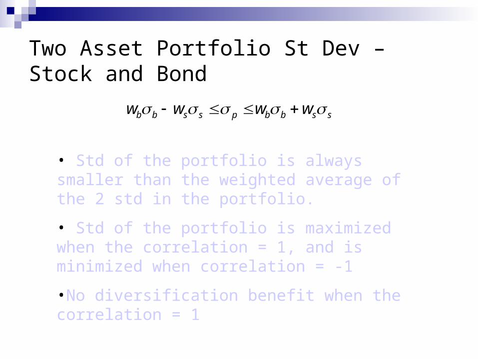
Two Asset Portfolio St Dev – Stock and Bond

ssbbpssbb wwww

• Std of the portfolio is always smaller than the weighted average of the 2 std in the portfolio.

• Std of the portfolio is maximized when the correlation = 1, and is minimized when correlation = -1

•No diversification benefit when the correlation = 1

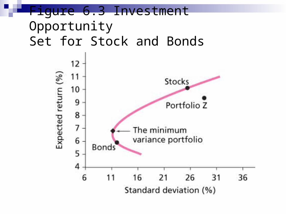
Figure 6.3 Investment Opportunity Set for Stock and Bonds

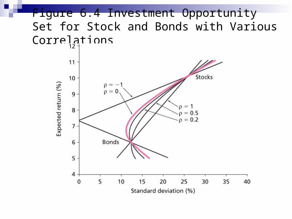
Figure 6.4 Investment Opportunity Set for Stock and Bonds with Various Correlations

6.3 THE OPTIMAL RISKY PORTFOLIO WITH A RISK-FREE ASSET

Extending to Include Riskless Asset The optimal combination becomes linear A single combination of risky and riskless

assets will dominate

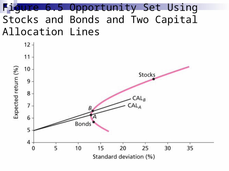
Figure 6.5 Opportunity Set Using Stocks and Bonds and Two Capital Allocation Lines

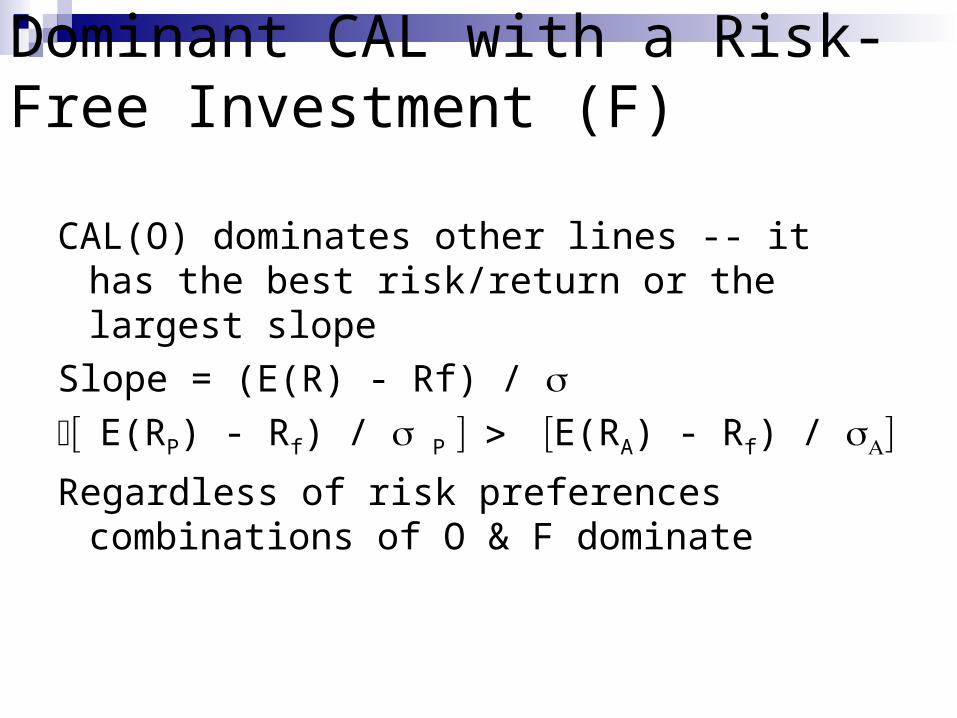
Dominant CAL with a Risk-Free Investment (F)

CAL(O) dominates other lines -- it has the best risk/return or the largest slope

Slope = (E(R) - Rf) / E(RP) - Rf) / PE(RA) - Rf) /

Regardless of risk preferences combinations of O & F dominate

Figure 6.6 Optimal Capital Allocation Line for Bonds, Stocks and T-Bills

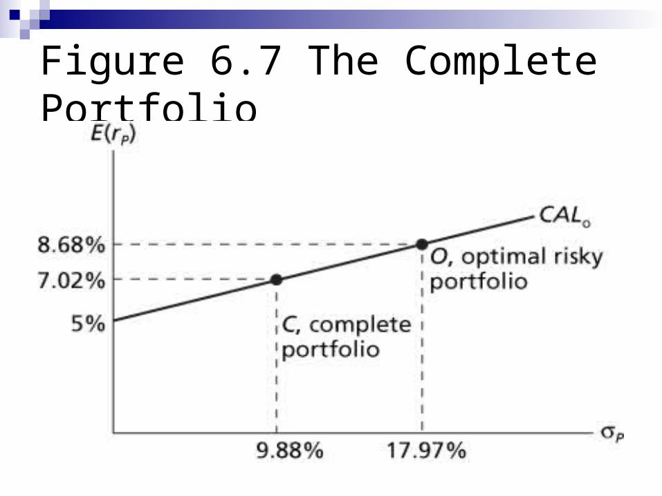
Figure 6.7 The Complete Portfolio

Figure 6.8 The Complete Portfolio – Solution to the Asset Allocation Problem

6.4 EFFICIENT DIVERSIFICATION WITH MANY RISKY ASSETS

Extending Concepts to All Securities

The optimal combinations result in lowest level of risk for a given return

The optimal trade-off is described as the efficient frontier

These portfolios are dominant

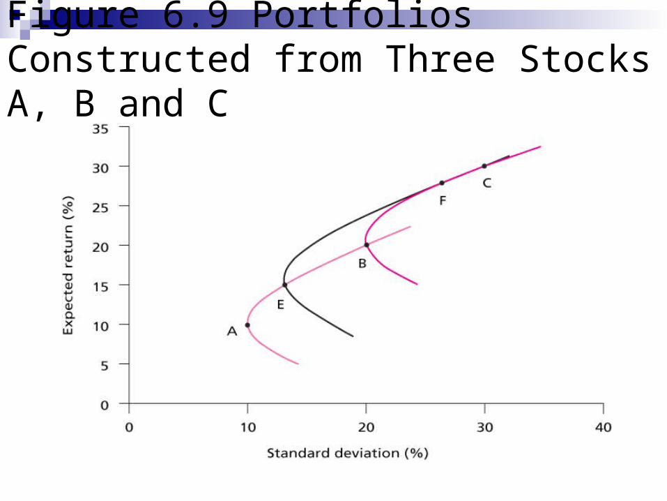
Figure 6.9 Portfolios Constructed from Three Stocks A, B and C

Figure 6.10 The Efficient Frontier of Risky Assets and Individual Assets

Portfolio Selection

Asset allocation Security selection

These two are separable!

Asset Allocation

“Asset allocation accounts for 94% of the differences in pension fund performance”

Identify investment opportunities (risk-return combinations)

Choose the optimal combination according to investor’s risk attitude

Optimal Portfolio Construction

Step 1: Using available risky securities (stocks) to construct efficient frontier.

Step 2: Find the optimal risky portfolio using risk-free asset

Step 3: Now We have a risk-return tradeoff, choose your most favorable asset allocation

ExpectedPortfolio Return, rp

Risk, p

Efficient Set

Feasible Set

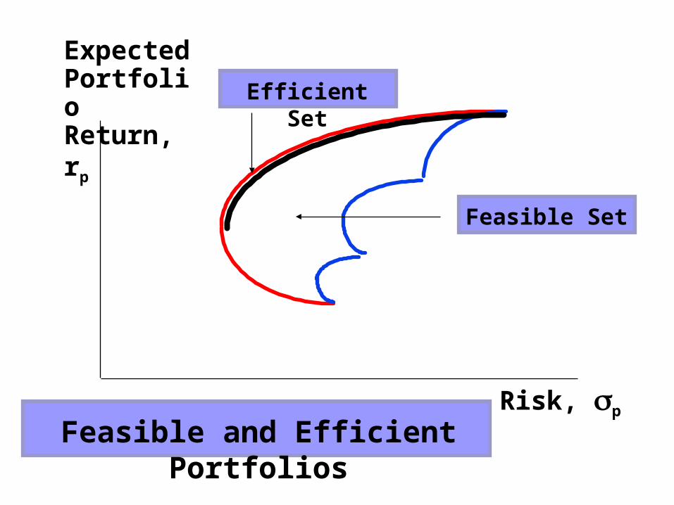
Feasible and Efficient Portfolios

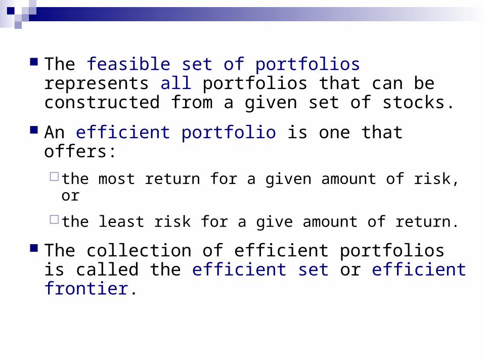
The feasible set of portfolios represents all portfolios that can be constructed from a given set of stocks.

An efficient portfolio is one that offers: the most return for a given amount of risk, or

the least risk for a give amount of return.

The collection of efficient portfolios is called the efficient set or efficient frontier.

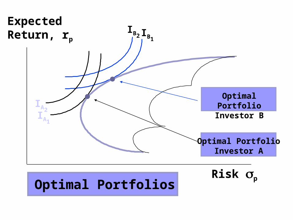
IB2 IB1

IA2IA1

Optimal PortfolioInvestor A

Optimal Portfolio

Investor B

Risk p

ExpectedReturn, rp

Optimal Portfolios

When a risk-free asset is added to the feasible set, investors can create portfolios that combine this asset with a portfolio of risky assets.

The straight line connecting rRF with M, the tangency point between the line and the old efficient set, becomes the new efficient frontier.

What impact does rRF have onthe efficient frontier?

M

Z

.ArRF

M Risk, p

Efficient Set with a Risk-Free Asset

The Capital MarketLine (CML):

New Efficient Set

..B

rM^

ExpectedReturn, rp

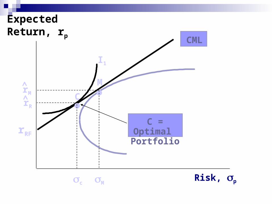
The Capital Market Line (CML) is all linear combinations of the risk-free asset and Portfolio M.

Portfolios below the CML are inferior.The CML defines the new efficient set.All investors will choose a portfolio on the

CML.

What is the Capital Market Line?

rRF

MRisk, p

I1

CML

C = Optimal Portfolio

.C .MrR

rM

c

^

^

ExpectedReturn, rp

Disadvantages of the efficient frontier approach

The efficient frontier was introduced by Markowitz (1952) and later earned him a Nobel prize in 1990.

However, the approach involved too many inputs, calculations If a portfolio includes only 2 stocks, to calculate the variance of the

portfolio, how many variance and covariance you need?

If a portfolio includes only 3 stocks, to calculate the variance of the portfolio, how many variance and covariance you need?

If a portfolio includes only n stocks, to calculate the variance of the portfolio, how many variance and covariance you need?

n variances n(n-1)/2 covariances

Single index model

level firm at they uncertaint toduereturn ofcomponent :

levelmarket at they uncertaint toduereturn ofcomponent :

market the toistock of nessresponsive :

intercept :

market of premiumrisk :

istock of premiumrisk :

i

mi

i

i

m

i

mm

ii

imiii

e

R

R

R

rfrR

rfrR

eRR

Single index model

risk specific :

componentrisk systematic :

risk Total:

2

22

2

2222

ei

mi

i

eimii

When we diversify, all the specific risk will go away, the only risk left is systematic risk component

22221

2 .......... mnmp

Now, all we need is to estimate beta1, beta2, ...., beta n, and the variance of the market. No need to calculate n variance, n(n-1)/2 covariances as before

Estimate beta

Run a linear regression according to the index model, the slope is the beta

For simplicity, we assume beta is the measure for market risk Beta = 0 Beta = 1 Beta > 1 Beta < 1

Advantages of the Single Index Model

Reduces the number of inputs for diversification

Easier for security analysts to specialize