4th

IASPEI / IAEE International Symposium:

Effects of Surface Geology on Seismic Motion

August 23–26, 2011 ∙ University of California Santa Barbara

ENHANCING SITE RESPONSE MODELING THROUGH DOWNHOLE ARRAY

RECORDINGS

Youssef M.A. Hashash David R. Groholski Byungmin Kim University of Illinois University of Illinois University of Illinois

Urbana-Champaign, IL 61801 Urbana-Champaign, IL 61801 Urbana-Champaign, IL 61801

USA USA USA

ABSTRACT

Laboratory tests are often used to understand dynamic soil behavior and to develop cyclic soil constitutive models. However, the

loading paths in lab tests are different from those in the field, resulting in the inaccurate prediction of site response. An increasing

number of downhole arrays are available to measure motions at the ground surface and within the soil profile, along with pore

pressure response within the soil profile. These downhole array recordings enhance our understanding of the wave propagation

through soils. This paper adapts the SelfSim inverse analysis framework to downhole array data to extract the nonlinear characteristics

of soil material while accounting for porewater pressure generation, and to improve site response modeling. Examples using

synthetically generated downhole array data and field array measurements are presented. The paper also presents preliminary analysis

of downhole array measurements from the recent 2011 Japan earthquake.

INTRODUCTION

Conventional site response analysis models are used to estimate seismic response at a site including acceleration, velocity, and

displacement at the ground surface and within the soil column. The quality of such an estimate highly depends on the representation of

cyclic soil behavior. Laboratory tests are often used to measure or evaluate dynamic soil behavior and then to develop cyclic soil

constitutive models. The loading paths in lab tests, however, are significantly different from those soil experienced in the field

(Kramer 1996) and are not necessarily representative of anticipated soil behavior under actual shaking. An increasing number of

downhole arrays are now available to measure motions at the ground surface and within the soil profile. These arrays provide valuable

data to enhance site response analysis models and reveal the in situ soil behavior under earthquake shaking. Nevertheless, learning

from field measurements is an inherently inverse problem that can be challenging to solve. Ad hoc approaches are sometimes adopted

to adjust soil model properties to match field observations, but these approaches are not always successful and do not necessarily

provide additional insight into the seismic site response or cyclic soil behavior.

Zeghal and Elgamal (1993) used a linear interpolation approach to estimate shear stress and strain seismic histories from downhole

arrays via a nonparametric system identification procedure. Another system identification approach, called parametric system

identification, such as time-domain method (Glaser and Baise 2000) and frequency domain method (Elgamal et al. 2001; Harichance

et al. 2005) has also been applied to downhole arrays. More recently Assimaki and Steidl (2007) developed a hybrid optimization

scheme for downhole array seismogram inversion. The proposed approach estimates the low-strain dynamic soil properties by the

inversion of low-amplitude waveforms and the equivalent linear dynamic soil properties by inversion of the mainshock. The results

have shown that that inversion of strong motion site response data may be used for the approximate assessment of nonlinear effects

experienced by soil formations during strong motion events. Current approaches, while providing important insights from field

observations, do not fully benefit from field observations. They are often constrained by prior assumptions about soil behavior or the

employed soil model.

2

SELFSIM INVERSE ANALYSIS FRAMEWORK

SelfSim inverse analysis framework is an extension of the autoprogressive algorithm originally proposed by Ghaboussi et al (1998).

With the use of a neural network (NN) based material model, the autoprogressive method is used to extract material behavior from

non-uniform material tests (Ghaboussi et al. 1998; Sidarta and Ghaboussi 1998). In a similar manner, the algorithm employed in

SelfSim extracts stress-strain material behavior using global load and deflection measurements. Hashash et al. (2003) further

developed this method to update constitutive models using measured deformations around an excavation. Using an incremental

nonlinear finite element analysis, two sets of boundaries (forces/displacements) are imposed in parallel with a parallel analysis

scheme. The parallel analyses yield stress-strain pairs that are used to train the NN material model. The procedure is repeated until

there is an acceptable match between the two analyses. The resulting NN model can then be used in the forward analysis of new

boundary value problems.

Total stress analysis

SelfSim allows for the extraction of the stress-strain field of a material from a general boundary value problem and provides a rich

data set in which to train a a continuously evolving NN based material model. Further research by Tsai and Hashash (2008) extended

the framework to the extraction of the stress-strain field from dynamic problems that were limited to total stress analysis. The concept

of extending SelfSim from static to dynamic problems is realized by recognizing that the loading (e.g. construction) steps of static

problems are analogous to the loading steps (equal to the number of time steps) of dynamic problems. Two parallel boundary

condition site response analyses are performed with NN based constitutive models to simulate the soil behavior. Initially, the soil

response is unknown and the NN soil models are pre-trained using stress-strain data that reflect viscous linear elastic response over a

limited strain range. The applicability of the framework to total stress site response analysis is demonstrated in synthetic arrays (Tsai

and Hashash 2008) as well as field arrays from the Lotung and La Cienaga arrays (Tsai and Hashash 2009) to extract and evaluate the

in situ soil behavior.

Site response analysis with pore water pressure

Similar to the application to total stress site response analysis, the dynamic problem can be treated as a number of incrementally

applied loading steps equal to the number of time steps. Figure 1 shows the concept of SelfSim applied to the downhole array problem

with inclusion of pore water pressure response. In Step 1, measurements of accelerations and pore pressures are gathered from the

downhole array instrumentation. The displacement boundary condition is established from the double integration of acceleration

measurements. Ground motion response is simulated using a modified version of the 1D nonlinear time domain component of the

DEEPSOIL code (Hashash and Park 2001).

In a typical 1D seismic site response problem, a seismic motion is propagated from the bottom of the soil profile to the ground surface.

In a downhole array the ground response corresponding to base shaking is measured at selected depths within the soil profile. The

input base shaking and the corresponding measurements within the soil profile yield complementary sets of field observations.

SelfSim uses these measurements to extract the underlying dynamic soil behavior. The parallel boundary condition analyses

performed within SelfSim consist of the force boundary conditions applied in one analysis, referred to as Step 2a, and displacement

boundary conditions applied in the other analysis, referred to as Step 2b.

The stresses from Step 2a and the strains from Step 2b form stress–strain pairs that approximate the soil constitutive response. The

material constitutive model is updated by training and retraining the NN based material model using the extracted stress-strain pairs.

The entire process is repeated several times using the full ground motion time series until analyses of Step 2a provide ground response

similar to the measured response. SelfSim has extracted sufficient information about the dynamic soil response to reproduce the field

measurements.

In order to implement SelfSim algorithm for fully-coupled seismic site response the following is needed:

1. A 1D site response analysis procedure for Step (2a) which includes the effects of pore pressures

2. A 1D site response analysis procedure for Step (2b) which includes the effects of pore pressures

3. A NN material model architecture that is capable of representing cyclic soil behavior and pore pressure response.

Site response analyses of Step 2a & 2b are again performed using a modified version of the 1-D non-linear time-domain component of

the DEEPSOIL code (Hashash and Park 2001).

3

1. Field measurements

2. SelfSim learning

(a) Simulate wave propagation

--Impose recorded pwp data

--Extract stresses

pi

(b) Apply measurements

--Extract calculated pwp

--Extract strains

3. Forward analysis with

extracted NN models

Other events

Stress-Strain, PWP data for initial NN

training:

1.Linear elastic

2.Laboratory tests

3.Case histories

4.Approximate constitutive models

p

Stress-Strain, PWP

Training of NANN

NANN based constitutive model

NANN based constitutive model

Soil NANN PWP NANN

pc

1. Field measurements1. Field measurements

2. SelfSim learning2. SelfSim learning

(a) Simulate wave propagation

--Impose recorded pwp data

--Extract stresses

(a) Simulate wave propagation

--Impose recorded pwp data

--Extract stresses

pipi

(b) Apply measurements

--Extract calculated pwp

--Extract strains

(b) Apply measurements

--Extract calculated pwp

--Extract strains

3. Forward analysis with

extracted NN models

Other events

3. Forward analysis with

extracted NN models

Other events

Stress-Strain, PWP data for initial NN

training:

1.Linear elastic

2.Laboratory tests

3.Case histories

4.Approximate constitutive models

p

Stress-Strain, PWP data for initial NN

training:

1.Linear elastic

2.Laboratory tests

3.Case histories

4.Approximate constitutive models

p

Stress-Strain, PWP

Training of NANN

NANN based constitutive model

NANN based constitutive model

Soil NANN PWP NANN

Stress-Strain, PWP

Training of NANN

NANN based constitutive model

NANN based constitutive model

Soil NANN PWP NANN

pcpc

Fig. 1 SelfSim algorithm applied to a downhole array.

The successful inclusion of multiple data types within the SelfSim analysis framework first requires an understanding of how and

where such data types are calculated within the modeled soil profile. There are two types of data considered within the analysis: (1)

data calculated by solving the equation of motion [e.g. acceleration, velocity, and displacement], and (2) data calculated from the

constitutive models employed in analysis [e.g. shear strain, shear stress, excess pore pressure]. The first data type is calculated at the

top of each modeled layer in the analysis which is referred to as a computation node. The second data type is calculated at the mid-

point of each modeled layer and is referred to as an integration point. By definition, a computation node cannot exist at the same

location as an integration point.

The imposition of measured excess pore pressures and displacements in Step 2a and Step 2b respectively raises an analytical issue

within the SelfSim framework if both measurements are available at the same depths within the soil profile. This is due to the fact that

the determination of excess pore pressure, shear stress, and shear strain occurs at integration points located at the mid-point of each

layer, while displacements occur at computational nodes located at the top of each layer. Thus, to make use of all available data, the

mesh discretization for Step 2a and Step 2b must differ.

Measured pore pressures are imposed in Step 2a, while measured displacements are imposed in Step 2b. Thus, what will be an

integration point in Step 2a will be a displacement node in Step 2b. This implies that integration points in the two analyses will not be

consistent, and thus data from these points cannot be used for training. If a given soil layer is represented as a single layer in Step 2a,

then it must be sub-divided into two layers in Step 2b. However, if this is done, the integration points for the layer will not match

between analyses, and no training could occur for this layer. Additional sub-layers are required for these layers if any training is to

occur. Layers which contain only a single type of measurement (i.e. displacement or pore pressure) do not need to be subdivided.

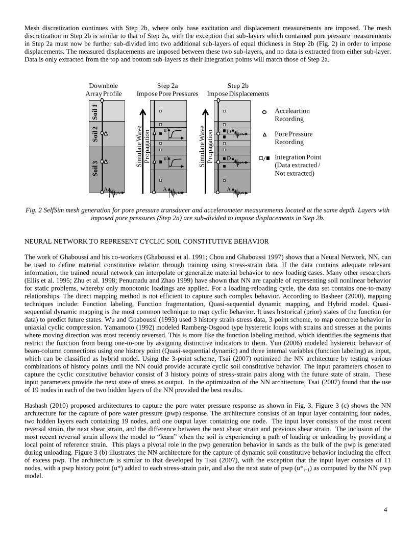
Figure 2 illustrates the development of the mesh generation for Step 2a and Step 2b for a downhole array with pore pressure and

acceleration measurements located at similar depths in the soil profile. In this consideration, a downhole array profile consisting of 3

soils (Soil1, Soil 2, Soil 3) has measurements of pore pressure and acceleration at the same depths in Soil 2 and Soil 3.

Mesh discretization begins with Step 2a, where only base excitation and pore pressure measurements are imposed. The discretization

of Soil 1 remains intact as there are no measurements in this layer. For Soil 2 and Soil 3, the soil layers are each discretized into 3 sub-

layers (Fig. 2) which will each employ the soil-specific NN for each sub-layer. The pore pressure measurement is imposed in the

second sub-layer and no data is extracted from this sub-layer. Training data for the soil is only extracted from the first and third sub-

layers, as these integration points will match those of Step 2b.

4

Mesh discretization continues with Step 2b, where only base excitation and displacement measurements are imposed. The mesh

discretization in Step 2b is similar to that of Step 2a, with the exception that sub-layers which contained pore pressure measurements

in Step 2a must now be further sub-divided into two additional sub-layers of equal thickness in Step 2b (Fig. 2) in order to impose

displacements. The measured displacements are imposed between these two sub-layers, and no data is extracted from either sub-layer.

Data is only extracted from the top and bottom sub-layers as their integration points will match those of Step 2a.

Downhole

Array ProfileS

oil

1S

oil

2S

oil

3

A A

u′

u′

Step 2a

Impose Pore Pressures

Sim

ula

te W

ave

Pro

pag

ati

on

Step 2b

Impose Displacements

A

D

D

Sim

ula

te W

ave

Pro

pag

ati

on

Acceleartion

Recording

Pore Pressure

Recording

Integration Point

(Data extracted /

Not extracted)

/

Fig. 2 SelfSim mesh generation for pore pressure transducer and accelerometer measurements located at the same depth. Layers with

imposed pore pressures (Step 2a) are sub-divided to impose displacements in Step 2b.

NEURAL NETWORK TO REPRESENT CYCLIC SOIL CONSTITUTIVE BEHAVIOR

The work of Ghaboussi and his co-workers (Ghaboussi et al. 1991; Chou and Ghaboussi 1997) shows that a Neural Network, NN, can

be used to define material constitutive relation through training using stress-strain data. If the data contains adequate relevant

information, the trained neural network can interpolate or generalize material behavior to new loading cases. Many other researchers

(Ellis et al. 1995; Zhu et al. 1998; Penumadu and Zhao 1999) have shown that NN are capable of representing soil nonlinear behavior

for static problems, whereby only monotonic loadings are applied. For a loading-reloading cycle, the data set contains one-to-many

relationships. The direct mapping method is not efficient to capture such complex behavior. According to Basheer (2000), mapping

techniques include: Function labeling, Function fragmentation, Quasi-sequential dynamic mapping, and Hybrid model. Quasi-

sequential dynamic mapping is the most common technique to map cyclic behavior. It uses historical (prior) states of the function (or

data) to predict future states. Wu and Ghaboussi (1993) used 3 history strain-stress data, 3-point scheme, to map concrete behavior in

uniaxial cyclic compression. Yamamoto (1992) modeled Ramberg-Osgood type hysteretic loops with strains and stresses at the points

where moving direction was most recently reversed. This is more like the function labeling method, which identifies the segments that

restrict the function from being one-to-one by assigning distinctive indicators to them. Yun (2006) modeled hysteretic behavior of

beam-column connections using one history point (Quasi-sequential dynamic) and three internal variables (function labeling) as input,

which can be classified as hybrid model. Using the 3-point scheme, Tsai (2007) optimized the NN architecture by testing various

combinations of history points until the NN could provide accurate cyclic soil constitutive behavior. The input parameters chosen to

capture the cyclic constitutive behavior consist of 3 history points of stress-strain pairs along with the future state of strain. These

input parameters provide the next state of stress as output. In the optimization of the NN architecture, Tsai (2007) found that the use

of 19 nodes in each of the two hidden layers of the NN provided the best results.

Hashash (2010) proposed architectures to capture the pore water pressure response as shown in Fig. 3. Figure 3 (c) shows the NN

architecture for the capture of pore water pressure (pwp) response. The architecture consists of an input layer containing four nodes,

two hidden layers each containing 19 nodes, and one output layer containing one node. The input layer consists of the most recent

reversal strain, the next shear strain, and the difference between the next shear strain and previous shear strain. The inclusion of the

most recent reversal strain allows the model to “learn” when the soil is experiencing a path of loading or unloading by providing a

local point of reference strain. This plays a pivotal role in the pwp generation behavior in sands as the bulk of the pwp is generated

during unloading. Figure 3 (b) illustrates the NN architecture for the capture of dynamic soil constitutive behavior including the effect

of excess pwp. The architecture is similar to that developed by Tsai (2007), with the exception that the input layer consists of 11

nodes, with a pwp history point (u*) added to each stress-strain pair, and also the next state of pwp (u*i+1) as computed by the NN pwp

model.

5

strain

stress

3 history points

,pi),( ii

,pi-1),( 11 -- ii

, pi-2),( 22 -- ii

,?), pi+1( 1+i

(i, i, pi), (i-1, i-1, pi-1), (i-2, i-2, pi-2), (i+1 , pi+1)

i+1SOIL NN Output layer

(1 node)

Hidden Layers(19 nodes ea.)

Input Layer(11 nodes)

(|i|, |rev|, i - rev), (|i+1|)

DpPWP NN Output layer

(1 node)

Hidden Layers

(19 nodes ea.)

Input Layer(4 nodes)

pi+1 = pi + Dp

(a)

(b)

(c)

Fig. 3 3-point model demonstrated for stress-strain-pore pressure coupled behavior (a). Proposed NN architectures for (b) pore

pressure response model, and (c) stress-strain model illustrating how the pore pressure output is given as input to the soil model.

SELFSIM LEARING USING DOWNHOLE ARRAY WITH POREWATER PRESSURE GENERATION

Synthetically generated downhole array data

The SelfSim learning of global measured responses while extracting the underlying soil behavior from downhole array measurements

is demonstrated using synthetically generated downhole array data. The advantage of using synthetically generated array data is that

soil behavior is known in advance and can be used to evaluate the extracted NN soil model. Development of synthetic vertical array

data follows three steps:

1. Select a soil profile with known nonlinear soil behavior at the site. The hyperbolic model in DEEPSOIL describes the

dynamic soil behavior. The Dobry-Matasovic model is used to describe the pore pressure response. Model parameters of the

hyperbolic model used for soil columns correspond to the nonlinear soil properties of Seed & Idriss curves for mean sands,

with pore pressure parameters corresponding to the sands present at the Wildlife Site in California.

2. Use DEEPSOIL to propagate a motion at bedrock through soil columns with known soil behavior using the hyperbolic soil

model.

3. The output displacement, velocity, acceleration, and pore water pressure data of certain layers are used as synthetic array

data.

A broadband input motion recorded during the Loma Gilroy earthquake which covers a wide range of frequencies is used to generate

synthetic recordings in a numerically modeled soil profile at the ground surface, Fig. 4 (a). The 40ft soil column is subdivided into 4

layers so that the maximum propagated frequency is at least 25 Hz. Although soil properties are uniform at the site, soils within

different sub-layers experience different loading paths.

Prior to SelfSim learning, the NN material models are initialized to represent linear elastic behavior with inclusion of degradation

within a limited strain range. The same NN material models are used for all layers. The computed surface motion using the initialized

model is different from the measurements (target) as shown in Fig. 5(a) which plots the ground surface acceleration, and Fig. 6 which

plots the surface response spectra. Figure 5 (a) shows that that initialized NN material models can predict the ground response during

the initial weak shaking (up to ~3 seconds), but cannot predict the behavior over the entire recorded ground motion.

6

(a)

Acceleration Recording

Pore Pressure Recording

u′

So

il 1

-V

s=

10

00

ft/

sec

10 f

t10 f

t10 f

t10 f

t

u′

0

1

2

3

4

5

6

7

8

0 100 200 300 400 500

0

1

2

3

4

5

6

7

8

Vs (m/s)

Silt (above GWT)

Silt (below GWT)

Silty Sand (WSB)

Silty Sand (WSA)

NN1

NN2

NN3

NN4

0

1

2

3

4

5

6

7

8

0 100 200 300 400 500

0

1

2

3

4

5

6

7

8

Vs (m/s)

Silt (above GWT)

Silt (below GWT)

Silty Sand (WSB)

Silty Sand (WSA)

NN1

NN2

NN3

NN4

Dep

th (

m)

Accelerometer

(b)

Fig. 4 (a) Soil profile of synthetic vertical array; (b) Geology and shear wave profile of Wildlife Liquefaction Array and four assigned

NN models according to the geology profile. Accelerometers are located at the top and bottom of the considered profile. Pore

pressure measurement locations are denoted as P1, P2, and P3.

SelfSim learning is divided into 2 windows for this event based on the amplitude of the motion as shown in Fig. 5 (a). Once SelfSim

learning can match the measurement for a given window, then SelfSim learning is continued for the next window:

SelfSim Learning, window 1: After six SelfSim learning passes (Fig. 5(b)), calculated surface accelerations approach the target

measurements within this window and can well predict the response at later shaking stages. During this window significant nonlinear

behavior and pore pressure response has been learned, and the analysis can proceed to the next training window.

SelfSim Learning, window 2: Four additional SelfSim learning passes are then performed using window 2 data (the entire period of

shaking). The computed response (Pass 10) matches acceleration measurements (Fig. 5 (c)) and the surface response (Fig. 6) very

well.

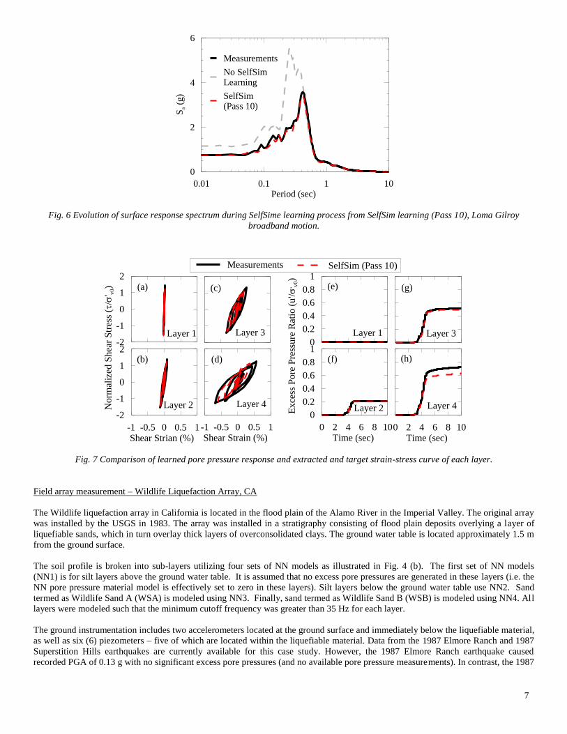
It appears that SelfSim is able to extract sufficient information about the soil behavior to accurately reproduce the field measurements.

The extracted stress-strain history and pore pressure response is compared to the known target soil response in Fig. 7. Although the

extracted behavior does not exactly match the target behavior there is an overall good match with the target response.

0 2 4 6 8 10Time (sec)

-1.5

-1

-0.5

0

0.5

1

1.5

Acc

eler

atio

n (

g)

0 2 4 6 8 10Time (sec)

Measurements

SelfSim

0 2 4 6 8 10Time (sec)

Window 1 Window 2

No SelfSimLearning

Pass 6 Pass 10(a) (b) (c)

Fig. 5 SelfSim learning of surface accelerations, Loma Gilroy broadband motion.

7

0.01 0.1 1 10Period (sec)

0

2

4

6

Sa

(g)

Measurements

No SelfSim Learning

SelfSim (Pass 10)

Fig. 6 Evolution of surface response spectrum during SelfSime learning process from SelfSim learning (Pass 10), Loma Gilroy

broadband motion.

0

0.2

0.4

0.6

0.8

1

-2

-1

0

1

2

Measurements SelfSim (Pass 10)

0 2 4 6 8 10Time (sec)

0

0.2

0.4

0.6

0.8

1

-1 -0.5 0 0.5 1Shear Strian (%)

-2

-1

0

1

2

0 2 4 6 8 10Time (sec)

-1 -0.5 0 0.5 1Shear Strain (%)

Norm

aliz

ed S

hea

r S

tres

s (

/' v

0)

Ex

cess

Po

re P

ress

ure

Rat

io (

u'/

' v0)

(a)

(b)

(c)

(d) (h)

(g)

(f)

(e)

Layer 1

Layer 2

Layer 3

Layer 4 Layer 4

Layer 3

Layer 2

Layer 1

Fig. 7 Comparison of learned pore pressure response and extracted and target strain-stress curve of each layer.

Field array measurement – Wildlife Liquefaction Array, CA

The Wildlife liquefaction array in California is located in the flood plain of the Alamo River in the Imperial Valley. The original array

was installed by the USGS in 1983. The array was installed in a stratigraphy consisting of flood plain deposits overlying a layer of

liquefiable sands, which in turn overlay thick layers of overconsolidated clays. The ground water table is located approximately 1.5 m

from the ground surface.

The soil profile is broken into sub-layers utilizing four sets of NN models as illustrated in Fig. 4 (b). The first set of NN models

(NN1) is for silt layers above the ground water table. It is assumed that no excess pore pressures are generated in these layers (i.e. the

NN pore pressure material model is effectively set to zero in these layers). Silt layers below the ground water table use NN2. Sand

termed as Wildlife Sand A (WSA) is modeled using NN3. Finally, sand termed as Wildlife Sand B (WSB) is modeled using NN4. All

layers were modeled such that the minimum cutoff frequency was greater than 35 Hz for each layer.

The ground instrumentation includes two accelerometers located at the ground surface and immediately below the liquefiable material,

as well as six (6) piezometers – five of which are located within the liquefiable material. Data from the 1987 Elmore Ranch and 1987

Superstition Hills earthquakes are currently available for this case study. However, the 1987 Elmore Ranch earthquake caused

recorded PGA of 0.13 g with no significant excess pore pressures (and no available pore pressure measurements). In contrast, the 1987

8

Superstition Hills earthquake had recorded PGA of 0.21 g and generated significant excess pore pressures to the extent of liquefaction

(u*

= u'⁄σ'v0 = 1). This evaluation has the potential to give significant insight into factors affecting modulus degradation and generation

of excess pore pressures for liquefiable sands.

Three scenarios using the Superstition Hills N-S earthquake measurements are considered in this investigation:

SH1 – Imposed Recordings, Linear Elastic NN Initialization

In this case, the measured ground surface displacements and pore pressure recordings from the Superstition Hills Earthquake are

implemented in SelfSim analysis to extract the underlying soil behavior. The NN material models are initialized to represent linear

elastic behavior (with some degradation due to generation of excess pore pressures) over a limited strain range. Extracted behavior and

ground response is compared with the recordings where available.

SH2 – Imposed Recordings; PDHM / D-M PWP Computed Values NN Initialization

In this case, the measured ground surface displacements and pore pressure recordings from the Superstition Hills Earthquake are

imposed as in SH1. In this scenario, the NN material models are initialized using PDHM and D-M pore pressure results from a 1D

analysis. The results are again compared as in SH1.

SH3 – Imposed Recordings; PDHM / GMP PWP Computed Values NN Initialization

In this case, the measured ground surface displacements and pore pressure recordings from the Superstition Hills Earthquake are once

again implemented. The NN material models are initialized using PDHM and GMP pore pressure results from a 1D analysis. The

results are again compared as in SH1.

Comparison of the surface response with surface measurements, 1D site response analysis models, and SelfSim scenarios SH1, SH2,

and SH3 are shown in Fig. 8. In general, it can be seen that the 1D site response analysis models have a tendency to slightly

overestimate response at low period (T < 0.1 sec), greatly overestimate response at periods between 0.1 and 1 second, and then

underestimate response at periods greater than 1 second. However, SelfSim is able to more accurately capture the measured surface

response for all scenarios. In all SelfSim scenarios (SH1, SH2, SH3), the response has greatly improved for periods less than 1

second. Response is still underestimated at periods greater than 1 second, but does show vast improvement. It is interesting to note

that the results of SH2 and SH3 provide the best results, with SH2 providing only a slightly better match, whereas the results of SH1

seem to be the least accurate of the three scenarios. The implications of these results are being investigated under current research.

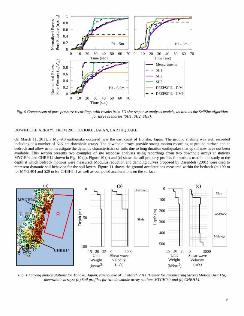
Excess pore pressure response from actual measurements, 1D site response analysis models, and SelfSim scenarios SH1, SH2, and

SH3 are shown in Fig. 9. It can be seen that the 1D site response analysis models are unable to represent the pore pressure

measurements for the complete duration. However, the D-M model does reasonably match measurements up to ~8 seconds of

shaking. At this point, it should be noted that it is now believed (Holzer and Youd 2007) that the interference of surface waves have

been the cause of delayed pore pressure response, followed by subsequent liquefaction of the sands after earthquake shaking had

ended. Thus, it is difficult to ascertain the validity of the use of either model in this case. However, once again we find that the results

of the SelfSim scenarios are able to more accurately learn the pore pressure generation behavior, though to varying degrees.

0.01 0.1 1 10Period (sec)

0

0.4

0.8

1.2

Sa

(g)

Measurements

Matasovic (1993)

DEEPSOIL - D/M

DEEPSOIL - GMP

SelfSim Learning - Std. Initialization

SelfSim Learning - D/M Initialization

SelfSim Learning - GMP Initialization

Fig. 8 Comparison of surface response spectra of surface measurements, results from 1D site response analysis models, and the

SelfSim algorithm for three scenarios (SH1, SH2, SH3) at the original Wildlife Site.

9

0 10 20 30 40 50 60 70Time (sec)

0

0.2

0.4

0.6

0.8

1

Norm

aliz

ed E

xce

ss

Pore

Pre

ssure

(u

x/

' v0)

Measurements

SH1

SH2

SH3

DEEPSOIL - D/M

DEEPSOIL - GMP

P1 - 5m

0 10 20 30 40 50 60 70Time (sec)

P2 - 3m

0 10 20 30 40 50 60 70Time (sec)

0

0.2

0.4

0.6

0.8

1

Norm

aliz

ed E

xce

ss

Pore

Pre

ssure

(u

x/

' v0)

P3 - 6.6m

Fig. 9 Comparison of pore pressure recordings with results from 1D site response analysis models, as well as the SelfSim algorithm

for three scenarios (SH1, SH2, SH3).

DOWNHOLE ARRAYS FROM 2011 TOHOKU, JAPAN, EARTHQUAKE

On March 11, 2011, a Mw=9.0 earthquake occurred near the east coast of Honshu, Japan. The ground shaking was well recorded

including at a number of KiK-net downhole arrays. The downhole arrays provide strong motion recording at ground surface and at

bedrock and allow us to investigate the dynamic characteristics of soils due to long duration earthquakes that up till now have not been

available. This section presents two examples of site response analyses using recordings from two downhole arrays at stations

MYGH04 and CHBH14 shown in Fig. 10 (a). Figure 10 (b) and (c) show the soil property profiles for stations used in this study to the

depth at which bedrock motions were measured. Modulus reduction and damping curves proposed by Darendeli (2001) were used to

represent dynamic soil behavior for the soil layers. Figure 11 shows the ground accelerations measured within the bedrock (at 100 m

for MYGH04 and 520 m for CHBH14) as well as computed accelerations on the surface.

(a)

MYGH04

CHBH14

Fill Soil

Shale

15 20 25Unit

Weight

(kN/m3)

100

50

0

Dep

th (

m)

0 3000Shear waveVelocity

(m/s)

Clay

Sandstone

15 20 25Unit

Weight

(kN/m3)

500

400

300

200

100

0

Dep

th (

m)

0 3000Shear waveVelocity

(m/s)

Melange

(b) (c)

Fig. 10 Strong motion stations for Tohoku, Japan, earthquake of 11 March 2011 (Center for Engineering Strong Motion Data) (a)

downwhole arrays; (b) Soil profiles for two downhole array stations MYGH04; and (c) CHBH14.

10

0 50 100 150 200 250 300Time (sec)

-0.5

0

0.5A

ccel

erat

ion

(g)

Surface (computed)

Surface (measured)

Bedrock motion

0 50 100 150 200 250 300Time (sec)

MYGH04 (EW) MYGH04 (NS)

0 50 100 150 200 250 300Time (sec)

-0.2

0

0.2

Acc

eler

atio

n (

g)

0 50 100 150 200 250 300Time (sec)

CHBH14 (EW) CHBH14 (NS)

Fig. 11 Accelerations measured within bedrock and computed on the surface, for stations MYGH04 and CHBH14.

The response spectra measured at the ground surface at station MYGH04 for two directions (EW and NS) are shown in Fig. 12. As a

rock site, the response spectra show the amplification of the high frequency components. These spectra were compared with computed

responses using the site response analysis program DEEPSOIL V4.0. It is noted that both equivalent-linear (EL) and nonlinear (NL)

analyses could capture the key features of the response, although some discrepancies are noted especially for the EW component.

Figure 13 shows the response spectra measured at the ground surface of station CHBH14 for two directions (EW and NS), compared

with the computed spectra. Similar to the case for MYGH04, the computed spectra capture key aspects of the response. However, the

computed spectra for this station overestimate the spectral accelerations at low frequency, especially for the EW direction. Further

work is currently under way to understand the sources of difference and try to enhance the site response analysis capability.

0.01 0.1 1 10Period (sec)

0

1

2

3

4

Sp

ectr

al a

ccel

erat

ion (

g) Computed_EL

Computed_NL

Measured_surface

Measured_bedrock

0.01 0.1 1 10Period (sec)

MYGH04 (EW) MYGH04 (NS)

Fig. 12 The response spectra measured at the ground surface of the station MYGH04 for two directions (EW and NS), compared with

the computed spectra using both equivalent-linear (EL) and nonlinear (NL) analyses.

11

0.01 0.1 1 10Period (sec)

0

0.4

0.8

1.2S

pec

tral

acc

eler

atio

n (

g)

Computed_EL

Computed_NL

Measured_surface

Measured_bedrock

0.01 0.1 1 10Period (sec)

CHBH14 (EW) CHBH14 (NS)

Fig. 13 The response spectra measured at the ground surface of the station CHBH14 for two directions (EW and NS), compared with

the computed spectra using both equivalent-linear (EQ) and nonlinear (NL) analyses.

CONCLUSIONS

An inverse analysis framework, SelfSim, is reviewed in the paper. The SelfSim has shown the capability of an evolving soil model to

reproduce global behavior of the site while simultaneously extracting the underlying soil behavior with pore water pressure response

using downhole array measurements unconstrained by prior assumptions of soil behavior.

The SelfSim algorithm is successfully demonstrated using one synthetic downhole array profile and one measurement from actual

field array (Wildlife Liquefaction Array, CA). A broadband input motion recorded during the Loma Gilroy earthquake was used for

synthetic downhole array profile which consists with 40ft soil column subdivided into 4 layers. The Superstition Hills N-S earthquake

measurements were used for the Wildlife liquefaction array in California. The results show that SelfSime is able to gradually learn the

measured global response while extracting the soil behavior and pore water pressure response.

Preliminary one-dimensional site response analyses were conducted using the program DeepSoil v4.0 to reproduce the soil response

from the downhole arrays for March 11 2011, Tohoku, Japan, earthquake. The ground motions measured within the soil profile were

used as input motions in site response analyses. Site response analysis is able to capture key features of the response.

REFERENCES

Assimaki, D. and Steidl, J. [2007]. "Inverse Analysis of Weak and Strong Motion Downhole Array Data from the Mw 7.0 Sanriku-

Minami Earthquake." Soil Dynamics and Earthquake Engineering 27: 73-92.

Basheer, I. A. [2000]. "Selection of Methodology for Neural Network Modeling of Constitutive Hystereses Bahavior of Soils."

Computer-Aided Civil and Infrastructure Engineering 15: 440-458.

Chou, J. H. and Ghaboussi, J. [1997]. Structural Damage Detection and Identification Using Genetic Algorithm. International

Conference on Artificial Neural Networks in Engineering, St. Louis, MO, ASME.

Darendeli, M. B. [2001]. Development of a New Family of Normalized Modulus Reduction and Material Damping Curves. Civil

Engineering. Austin, University of Texas at Austin: 395.

Elgamal, A., et al. [2001]. Dynamic Soil Properties, Seismic Downhole Arrays and Applications in Practice. 4th International

Conference on Recent Advances in Geotechnical Earthquake Engineering and Soil Dynamics, San Diego, California, USA, University

of Missouri-Rolla.

Ellis, G. W., et al. [1995]. "Stress-Strain Modeling of Sands Using Artifiical Neural Network." Journal of Geotechnical Engineering:

429-435.

Ghaboussi, J., et al. [1991]. "Knowledge-Based Modeling of Material Behavior with Neural Networks." Journal of Engineering

Mechanics-Asce 117(1): 132-153.

12

Ghaboussi, J., et al. [1998]. "Autoprogressive Training of Neural Network Constitutive Models." International Journal for Numerical

Methods in Engineering 42(1): 105-126.

Glaser, S. D. and Baise, L. G. [2000]. "System Identification Estimation of Soil Properties at the Lotung Site." Soil Dynamics and

Earthquake Engineering 19: 521-531.

Harichance, Z., et al. [2005]. "An Identification Procedure of Soil Profile Characteristics from Two Free Field Acclerometer Records."

Soil Dynamics and Earthquake Engineering 25: 431-438.

Hashash, Y. M. A. [2010]. Nonlinear Soil Behavior from Downhole Array Measurements and Site Response Modeling. U.S.

Geological Survey. Award No. 08hqgr0029.

Hashash, Y. M. A., et al. [2003]. "Temperature Correction and Strut Loads in Deep Excavations for the Central Artery Project."

Journal of Geotechnical and Geoenvironmental Engineering 129(6): pp. 495-505.

Hashash, Y. M. A. and Park, D. [2001]. "Non-Linear One-Dimensional Seismic Ground Motion Propagation in the Mississippi

Embayment." Engineering Geology 62(1-3): 185-206.

Holzer, T. L. and Youd, T. L. [2007]. "Liquefaction, Ground Oscillation, and Soil Deformation at the Wildlife Array, California."

Bulletin of the Seismological society of America 97(3): 961-976.

Kramer, S. L. [1996]. Geotechnical Earthquake Engineering. Upper Saddle River, N.J., Prentice Hall.

Penumadu, D. and Zhao, R. [1999]. "Triaxial Compression Behavior of Sand and Gravel Using Artificial Neural Networks (Ann)."

Computers and Geotechnics 24(3): 207-230.

Sidarta, D. and Ghaboussi, J. [1998]. "Modelling Constitutive Behavior of Materials from Non-Uniform Material Tests." Computers

and Geotechnics 22(1): 53-71.

Tsai, C.-C. [2007]. Seismic Site Response and Interpretation of Dynamic Soil Behavior from Downhole Array Measurements.

Department of Civil and Environmental Engineering. Urbana, University of Illinois at Urbana-Champaign.

Tsai, C.-C. and Hashash, Y. M. A. [2008]. "A Novel Framework Integrating Downhole Array Data and Site Response Analysis to

Extract Dynamic Soil Behavior." Soil Dynamics and Earthquake Engineering 28(3): 181-197.

Tsai, C.-C. and Hashash, Y. M. A. [2009]. "Learning of Dynamic Soil Behavior from Downhole Arrays." Journal of geotechincal and

geoenvironmental engineering 135(6): 745-757.

Wu, X. and Ghaboussi, J. [1993]. Modelling the Cyclic Behavior of the Concrete Using Adaptive Neural Networks. Asian Pacific

conference on computational mechanics.

Yamamoto, K. [1992]. Modeling of Hysteretic Behavior with Neural Network and Its Application to Non-Linear Dynamic Response,

proceedings of the international conference in applications of artificial intelligence in engineering.

Yun, G. J. [2006]. Modeling of Hysteretic Behavior of Beam-Column Connections Based on Self Learning Simulation. Civil and

Environmental Engineering. Urbana, University of Illinois at Urbana-Champaign.

Zeghal, M. and Elgamal, A.-W. [1993]. Lotung Sites: Downhole Seismic Data Analysis. Palo Alto, Calif,, Electric Power Research

Institute.

Zhu, J., et al. [1998]. "Modeling of Soil Behavior with a Recurrent Neural Network." Canadian Geotechnical Journal 35: 858-872.