Computers and Mathematics with Applications 61 (2011) 1442–1456

Contents lists available at ScienceDirect

Computers and Mathematics with Applications

journal homepage: www.elsevier.com/locate/camwa

Effects of slip on sheet-driven flow and heat transfer of anon-Newtonian fluid past a stretching sheetBikash Sahoo ∗

Department of Mathematics, National Institute of Technology, Rourkela, Rourkela-769008, India

a r t i c l e i n f o

Article history:Received 5 September 2009Received in revised form 10 January 2011Accepted 10 January 2011

Keywords:Third grade fluidPartial slipMagnetic fieldHeat transferHeat source (sink)Finite difference methodBroyden’s method

a b s t r a c t

The flow and heat transfer of an electrically conducting non-Newtonian fluid due to astretching surface subject to partial slip is considered. The constitutive equation of the non-Newtonian fluid is modeled by that for a third grade fluid. The heat transfer analysis hasbeen carried out for twoheating processes, namely, (i)with prescribed surface temperature(PST-case) and (ii) prescribed surface heat flux (PHFcase) in presence of a uniform heatsource or sink. Suitable similarity transformations are used to reduce the resulting highlynonlinear partial differential equations into ordinary differential equations. The issue ofpaucity of boundary conditions is addressed and an effective second order numericalscheme has been adopted to solve the obtained differential equations. The importantfinding in this communication is the combined effects of the partial slip, magnetic field,heat source (sink) parameter and the third grade fluid parameters on the velocity, skinfriction coefficient and the temperature field. It is interesting to find that slip decreases themomentum boundary layer thickness and increases the thermal boundary layer thickness,whereas the third grade fluid parameter has an opposite effect on the thermal and velocityboundary layers.

© 2011 Elsevier Ltd. All rights reserved.

1. Introduction

Boundary layer flow on a continuous moving surface has many practical applications in industrial manufacturingprocesses. Examples for such applications are: Aerodynamic extrusion of plastic sheets, cooling of infinite metallic plate ina cooling bath, the boundary layer along a liquid film in condensation processes, and a polymer sheet or filament extrudedcontinuously from a dye. Applications also include paper production and glass blowing. The analysis of boundary layerflows of viscous fluids driven by a moving surface dates back to the pioneering investigation by Sakiadis [1]. There aresituations when the extruded polymer sheet is being stretched as it is being extruded and this is bound to alter significantlythe boundary layer characteristics of the flow considered by Sakiadis.

The steady two-dimensional laminar flow of an incompressible, viscous fluid past a stretching sheet has become aclassical problem in fluid dynamics as it admits anunusual simple closed formsolution, first discoveredbyCrane [2]. The flowand heat transfer phenomena over a stretching surface have promising applications in a number of technological processesincluding the production of polymer films or thin sheets. Gupta and Gupta [3] examined the heat and mass transfer usinga similarity transformation subject to suction or blowing. In fact, realistically stretching of the sheet may not necessarilybe linear. This situation is dealt by many authors [4–6]. Moreover, the flow past a stretching sheet need not be necessarilytwo-dimensional because the stretching of the sheet can take place in a variety of ways. If the flow is not two-dimensional,an analytic solution in the closed form does not seem to exist [7–9].

All the above investigations were restricted to the flows of Newtonian fluids. A rigorous study of the boundary layerflow and heat transfer of different non-Newtonian fluids past a stretching sheet was required due to its immense industrial

∗ Tel.: +91 0661 246 2706.E-mail address: bikashsahoo@nitrkl.ac.in.

0898-1221/$ – see front matter© 2011 Elsevier Ltd. All rights reserved.doi:10.1016/j.camwa.2011.01.017

B. Sahoo / Computers and Mathematics with Applications 61 (2011) 1442–1456 1443

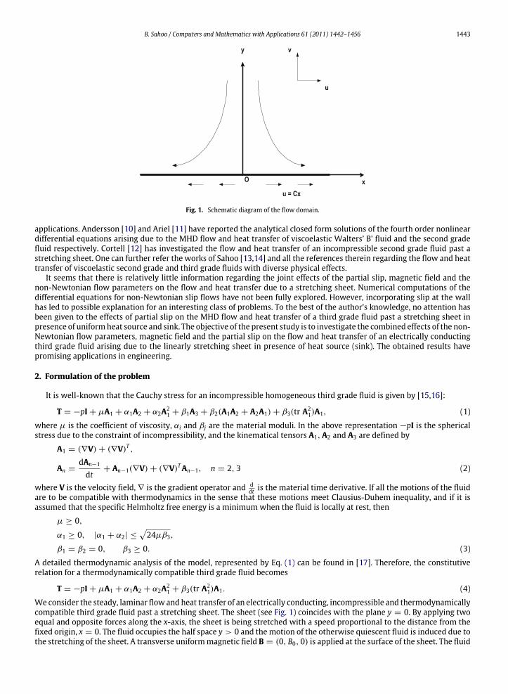
Fig. 1. Schematic diagram of the flow domain.

applications. Andersson [10] and Ariel [11] have reported the analytical closed form solutions of the fourth order nonlineardifferential equations arising due to the MHD flow and heat transfer of viscoelastic Walters’ B’ fluid and the second gradefluid respectively. Cortell [12] has investigated the flow and heat transfer of an incompressible second grade fluid past astretching sheet. One can further refer the works of Sahoo [13,14] and all the references therein regarding the flow and heattransfer of viscoelastic second grade and third grade fluids with diverse physical effects.

It seems that there is relatively little information regarding the joint effects of the partial slip, magnetic field and thenon-Newtonian flow parameters on the flow and heat transfer due to a stretching sheet. Numerical computations of thedifferential equations for non-Newtonian slip flows have not been fully explored. However, incorporating slip at the wallhas led to possible explanation for an interesting class of problems. To the best of the author’s knowledge, no attention hasbeen given to the effects of partial slip on the MHD flow and heat transfer of a third grade fluid past a stretching sheet inpresence of uniformheat source and sink. The objective of the present study is to investigate the combined effects of the non-Newtonian flow parameters, magnetic field and the partial slip on the flow and heat transfer of an electrically conductingthird grade fluid arising due to the linearly stretching sheet in presence of heat source (sink). The obtained results havepromising applications in engineering.

2. Formulation of the problem

It is well-known that the Cauchy stress for an incompressible homogeneous third grade fluid is given by [15,16]:

T = −pI + µA1 + α1A2 + α2A21 + β1A3 + β2(A1A2 + A2A1) + β3(tr A2

1)A1, (1)

where µ is the coefficient of viscosity, αi and βj are the material moduli. In the above representation −pI is the sphericalstress due to the constraint of incompressibility, and the kinematical tensors A1,A2 and A3 are defined by

A1 = (∇V) + (∇V)T ,

An =dAn−1

dt+ An−1(∇V) + (∇V)TAn−1, n = 2, 3 (2)

where V is the velocity field, ∇ is the gradient operator and ddt is the material time derivative. If all the motions of the fluid

are to be compatible with thermodynamics in the sense that these motions meet Clausius-Duhem inequality, and if it isassumed that the specific Helmholtz free energy is a minimum when the fluid is locally at rest, then

µ ≥ 0,

α1 ≥ 0, |α1 + α2| ≤24µβ3,

β1 = β2 = 0, β3 ≥ 0. (3)

A detailed thermodynamic analysis of the model, represented by Eq. (1) can be found in [17]. Therefore, the constitutiverelation for a thermodynamically compatible third grade fluid becomes

T = −pI + µA1 + α1A2 + α2A21 + β3(tr A2

1)A1. (4)

We consider the steady, laminar flow and heat transfer of an electrically conducting, incompressible and thermodynamicallycompatible third grade fluid past a stretching sheet. The sheet (see Fig. 1) coincides with the plane y = 0. By applying twoequal and opposite forces along the x-axis, the sheet is being stretched with a speed proportional to the distance from thefixed origin, x = 0. The fluid occupies the half space y > 0 and themotion of the otherwise quiescent fluid is induced due tothe stretching of the sheet. A transverse uniformmagnetic field B = (0, B0, 0) is applied at the surface of the sheet. The fluid

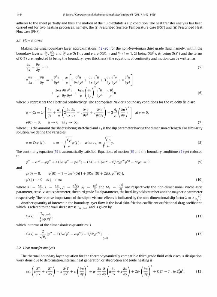
1444 B. Sahoo / Computers and Mathematics with Applications 61 (2011) 1442–1456

adheres to the sheet partially and thus, the motion of the fluid exhibits a slip condition. The heat transfer analysis has beencarried out for two heating processes, namely, the (i) Prescribed Surface Temperature case (PST) and (ii) Prescribed HeatFlux case (PHF).

2.1. Flow analysis

Making the usual boundary layer approximations [18–20] for the non-Newtonian third grade fluid, namely, within theboundary layer u, ∂u

∂x ,∂2u∂x2

and ∂p∂x are O(1), y and v are O(δ), ν and αi

ρ(i = 1, 2) being O(δ2), β3 being O(δ4) and the terms

of O(δ) are neglected (δ being the boundary layer thickness), the equations of continuity and motion can be written as

∂u∂x

+∂v

∂y= 0, (5)

u∂u∂x

+ v∂u∂y

= ν∂2u∂y2

+α1

ρ

u

∂3u∂x∂y2

+∂u∂x

∂2u∂y2

+ 3∂u∂y

∂2v

∂y2+ v

∂3u∂y3

+2α2

ρ

∂u∂y

∂2v

∂y2+

6β3

ρ

∂u∂y

2∂2u∂y2

−σB2

0

ρu (6)

where σ represents the electrical conductivity. The appropriate Navier’s boundary conditions for the velocity field are

u − Cx = λ1

∂u∂y

+α1

µ

2∂u∂x

∂u∂y

+ v∂2u∂y2

+ u∂2u∂x∂y

+ 2

β3

µ

∂u∂y

3at y = 0,

v(0) = 0, u → 0 as y → ∞ (7)

where C is the amount the sheet is being stretched and λ1 is the slip parameter having the dimension of length. For similaritysolution, we define the variables,

u = Cxϕ′(ζ ), v = −

Cµ

ρϕ(ζ ), where ζ =

Cρ

µy. (8)

The continuity equation (5) is automatically satisfied. Equations of motion (6) and the boundary conditions (7) get reducedto

ϕ′′′− ϕ′2

+ ϕϕ′′+ K(2ϕ′ϕ′′′

− ϕϕiv) − (3K + 2L)ϕ′′2+ 6βRxϕ

′′′ϕ′′2− Mnϕ

′= 0, (9)

and

ϕ(0) = 0, ϕ′(0) − 1 = λϕ′′(0)[1 + 3Kϕ′(0) + 2βRxϕ′′2(0)],

ϕ′(ζ ) → 0 as ζ → ∞ (10)

where K =Cα1µ

, L =Cα2µ

, β =C2β3

µ, Rx =

Cx2ν

and Mn =σB20ρC are respectively the non-dimensional viscoelastic

parameter, cross-viscous parameter, the third grade fluid parameter, the local Reynolds number and themagnetic parameter

respectively. The relative importance of the slip to viscous effects is indicated by the non-dimensional slip factor λ = λ1

Cν.

Another quantity of interest in the boundary layer flow is the local skin-friction coefficient or frictional drag coefficient,which is related to the wall shear stress Txy|y=0, and is given by

Cf (x) =Txy|y=012ρ(Cx)2

, (11)

which in terms of the dimensionless quantities is

Cf (x) =2

√Rx

[ϕ′′+ K(3ϕ′ϕ′′

− ϕϕ′′′) + 2βRxϕ′′3

]

ζ=0

. (12)

2.2. Heat transfer analysis

The thermal boundary layer equation for the thermodynamically compatible third grade fluid with viscous dissipation,work done due to deformation,internal heat generation or absorption and Joule heating is

ρcp

u∂T∂x

+ v∂T∂y

= κ

∂2T∂y2

+ µ

∂u∂y

2

+ α1∂u∂y

∂

∂y

u∂u∂x

+ v∂v

∂y

+ 2β3

∂u∂y

4

+ Q (T − T∞)σB20u

2. (13)

B. Sahoo / Computers and Mathematics with Applications 61 (2011) 1442–1456 1445

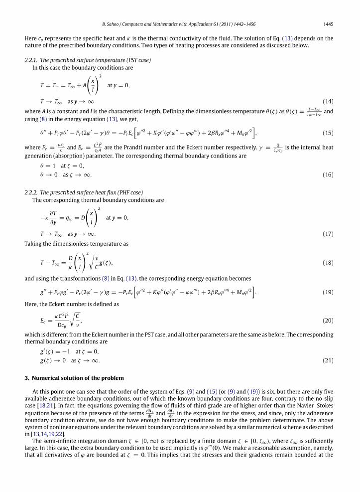
Here cp represents the specific heat and κ is the thermal conductivity of the fluid. The solution of Eq. (13) depends on thenature of the prescribed boundary conditions. Two types of heating processes are considered as discussed below.

2.2.1. The prescribed surface temperature (PST case)In this case the boundary conditions are

T = Tw = T∞ + A

xl

2

at y = 0,

T → T∞ as y → ∞ (14)

where A is a constant and l is the characteristic length. Defining the dimensionless temperature θ(ζ ) as θ(ζ ) =T−T∞Tw−T∞

andusing (8) in the energy equation (13), we get,

θ ′′+ Prϕθ ′

− Pr(2ϕ′− γ )θ = −PrEc

ϕ′′2

+ Kϕ′′(ϕ′ϕ′′− ϕϕ′′′) + 2βRxϕ

′′4+ Mnϕ

′2, (15)

where Pr =µcpκ

and Ec =C2 l2cpA

are the Prandtl number and the Eckert number respectively. γ =Q

Cρcpis the internal heat

generation (absorption) parameter. The corresponding thermal boundary conditions are

θ = 1 at ζ = 0,θ → 0 as ζ → ∞. (16)

2.2.2. The prescribed surface heat flux (PHF case)The corresponding thermal boundary conditions are

−κ∂T∂y

= qw = D

xl

2

at y = 0,

T → T∞ as y → ∞. (17)

Taking the dimensionless temperature as

T − T∞ =Dκ

xl

2ν

Cg(ζ ), (18)

and using the transformations (8) in Eq. (13), the corresponding energy equation becomes

g ′′+ Prϕg ′

− Pr(2ϕ′− γ )g = −PrEc

ϕ′′2

+ Kϕ′′(ϕ′ϕ′′− ϕϕ′′′) + 2βRxϕ

′′4+ Mnϕ

′2. (19)

Here, the Eckert number is defined as

Ec =κC2l2

Dcp

Cν

, (20)

which is different from the Eckert number in the PST case, and all other parameters are the same as before. The correspondingthermal boundary conditions are

g ′(ζ ) = −1 at ζ = 0,g(ζ ) → 0 as ζ → ∞. (21)

3. Numerical solution of the problem

At this point one can see that the order of the system of Eqs. (9) and (15) (or (9) and (19)) is six, but there are only fiveavailable adherence boundary conditions, out of which the known boundary conditions are four, contrary to the no-slipcase [18,21]. In fact, the equations governing the flow of fluids of third grade are of higher order than the Navier–Stokesequations because of the presence of the terms dA1

dt and dA2dt in the expression for the stress, and since, only the adherence

boundary condition obtains, we do not have enough boundary conditions to make the problem determinate. The abovesystemof nonlinear equations under the relevant boundary conditions are solved by a similar numerical scheme as describedin [13,14,19,22].

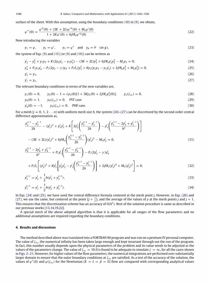
The semi-infinite integration domain ζ ∈ [0, ∞) is replaced by a finite domain ζ ∈ [0, ζ∞), where ζ∞ is sufficientlylarge. In this case, the extra boundary condition to be used implicitly is ϕ′′′(0). We make a reasonable assumption, namely,that all derivatives of ϕ are bounded at ζ = 0. This implies that the stresses and their gradients remain bounded at the

1446 B. Sahoo / Computers and Mathematics with Applications 61 (2011) 1442–1456

surface of the sheet. With this assumption, using the boundary conditions (10) in (9), we obtain,

ϕ′′′(0) =ϕ′2(0) + (3K + 2L)ϕ′′2(0) + Mnϕ

′(0)1 + 2Kϕ′(0) + 6βRxϕ′′2(0)

. (22)

Now introducing the variables

y1 = ϕ, y2 = ϕ′, y3 = ϕ′′ and y4 = θ (or g), (23)

the system of Eqs. (9) and (15) (or (9) and (19)) can be written as

y′

3 − y22 + y1y3 + K(2y2y′

3 − y1y′′

3) − (3K + 2L)y23 + 6βRxy′

3y23 − Mny2 = 0, (24)

y′′

4 + Pry1y′

4 − Pr(2y2 − γ )y4 + PrEc[y23 + Ky3(y2y3 − y1y′

3) + 2βRxy43 + Mny22] = 0, (25)

y′

2 = y3, (26)

y′

1 = y2. (27)

The relevant boundary conditions in terms of the new variables are,

y1(0) = 0, y2(0) − 1 = λy3(0)[1 + 3Ky2(0) + 2βRxy23(0)], y2(ζ∞) = 0, (28)

y4(0) = 1, y4(ζ∞) = 0, PST case (29)

y′

4(0) = −1, y4(ζ∞) = 0, PHF case. (30)

For a mesh (j = 0, 1, 2 . . . n) with uniformmesh size h, the system (24)–(27) can be discretized by the second order centraldifference approximation as,

yj+13 − yj−1

3

2h− (yj2)

2+ yj1y

j3 + K

2yj2

yj+13 − yj−1

3

2h

− yj1

yj+13 − 2yj3 + yj−1

3

h2

− (3K + 2L)(yj3)2+ 6βRx

yj+13 − yj−1

3

2h

(yj3)

2− Mny

j2 = 0, (31)

yj+14 − 2yj4 + yj−1

4

h2+ Pry

j1

yj+14 − yj−1

4

2h

− Pr(2y

j2 − γ )yj4

+ PrEc

(yj3)

2+ Kyj3

yj2y

j3 − yj1

yj+13 − yj−1

3

2h

+ 2βRx(y

j3)

4+ Mn(y

j2)

2

= 0, (32)

yj+12 = yj2 +

12h(yj3 + yj+1

3 ), (33)

yj+11 = yj1 +

12h(yj2 + yj+1

2 ). (34)

In Eqs. (24) and (25), we have used the central difference formula centered at the mesh point j. However, in Eqs. (26) and(27), we use the same, but centered at the point

j + 1

2

, and the average of the values of y at the mesh points j and j + 1.

This ensures that the discretization scheme has an accuracy of O(h2). Rest of the solution procedure is same as described inour previous works [13,14,19,22].

A special merit of the above adopted algorithm is that it is applicable for all ranges of the flow parameters and noadditional assumptions are required regarding the boundary conditions.

4. Results and discussions

Themethod described abovewas translated into a FORTRAN90 programandwas run on a pentium IV personal computer.The value of ζ∞, the numerical infinity has been taken large enough and kept invariant through out the run of the program.In fact, this number usually depends upon the physical parameters of the problem and its value needs to be adjusted as thevalues of the parameters change. The value of ζ∞ = 10.0 is found to be adequate to simulate ζ = ∞, for all the cases shownin Figs. 2–21. However, for higher values of the flowparameters, the numerical integrations are performed over substantiallylarger domain to ensure that the outer boundary conditions at ζ∞ are satisfied. As a test of the accuracy of the solution, thevalues of ϕ′′(0) and ϕ(ζ∞) for the Newtonian (K = L = β = 0) flow are compared with corresponding analytical values

B. Sahoo / Computers and Mathematics with Applications 61 (2011) 1442–1456 1447

reported by Wang [23,24]. It can be seen from the Table 1 that there is a good agreement between the numerical solutionobtained by the present algorithm and the exact analytical solution reported by Wang [23,24].

In order to have an insight of the flow and heat transfer characteristics, results are plotted graphically in Figs. 2–21 fordifferent choices of the flow parameters and a fixed value of the local Reynolds number Rx.

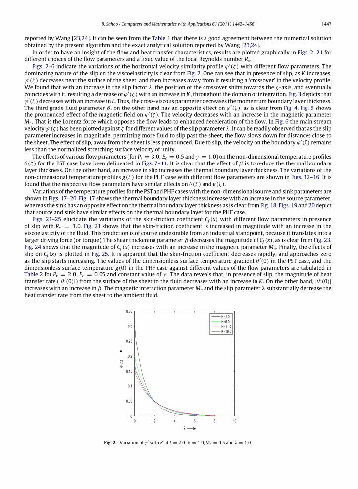
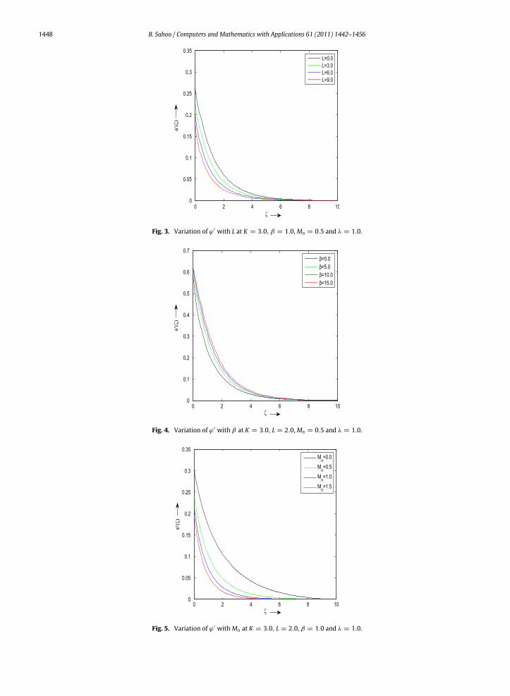
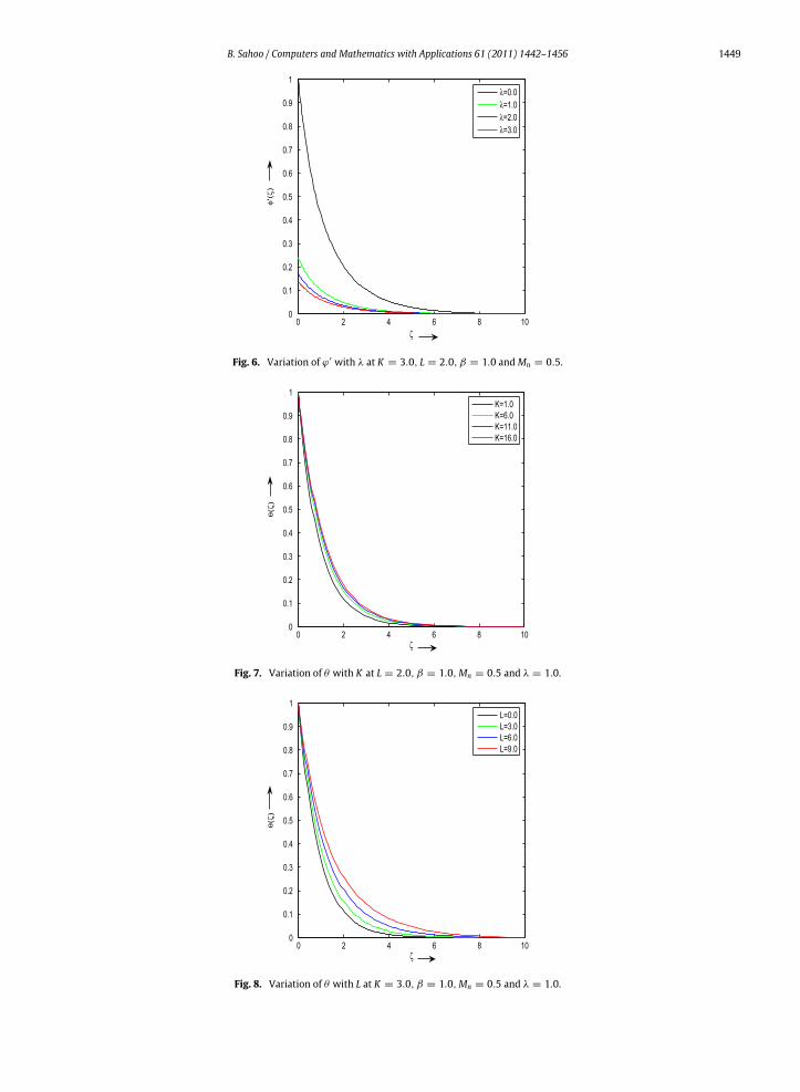
Figs. 2–6 indicate the variations of the horizontal velocity similarity profile ϕ′(ζ ) with different flow parameters. Thedominating nature of the slip on the viscoelasticity is clear from Fig. 2. One can see that in presence of slip, as K increases,ϕ′(ζ ) decreases near the surface of the sheet, and then increases away from it resulting a ‘crossover’ in the velocity profile.We found that with an increase in the slip factor λ, the position of the crossover shifts towards the ζ -axis, and eventuallycoincideswith it, resulting a decrease ofϕ′(ζ )with an increase in K , throughout the domain of integration. Fig. 3 depicts thatϕ′(ζ ) decreaseswith an increase in L. Thus, the cross-viscous parameter decreases themomentumboundary layer thickness.The third grade fluid parameter β , on the other hand has an opposite effect on ϕ′(ζ ), as is clear from Fig. 4. Fig. 5 showsthe pronounced effect of the magnetic field on ϕ′(ζ ). The velocity decreases with an increase in the magnetic parameterMn. That is the Lorentz force which opposes the flow leads to enhanced deceleration of the flow. In Fig. 6 the main streamvelocityϕ′(ζ ) has been plotted against ζ for different values of the slip parameterλ. It can be readily observed that as the slipparameter increases in magnitude, permitting more fluid to slip past the sheet, the flow slows down for distances close tothe sheet. The effect of slip, away from the sheet is less pronounced. Due to slip, the velocity on the boundary ϕ′(0) remainsless than the normalized stretching surface velocity of unity.

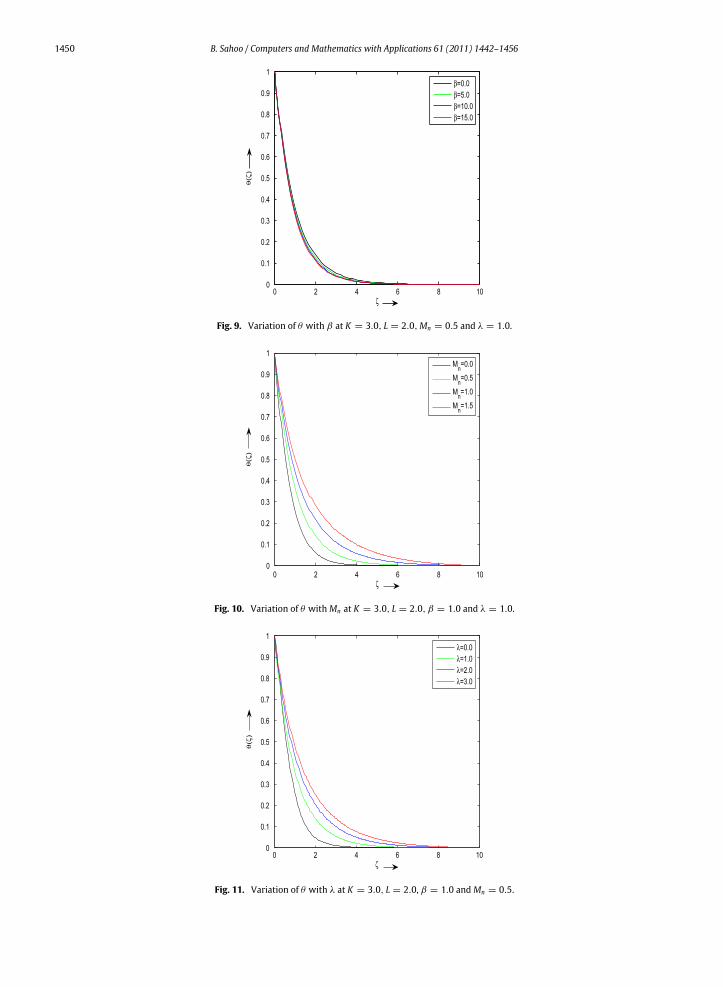
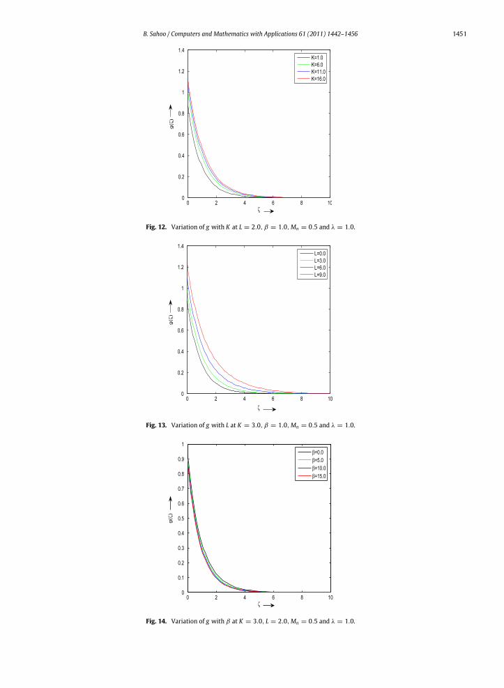
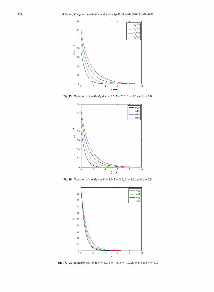
The effects of various flowparameters (for Pr = 3.0, Ec = 0.5 and γ = 1.0) on the non-dimensional temperature profilesθ(ζ ) for the PST case have been delineated in Figs. 7–11. It is clear that the effect of β is to reduce the thermal boundarylayer thickness. On the other hand, an increase in slip increases the thermal boundary layer thickness. The variations of thenon-dimensional temperature profiles g(ζ ) for the PHF case with different flow parameters are shown in Figs. 12–16. It isfound that the respective flow parameters have similar effects on θ(ζ ) and g(ζ ).

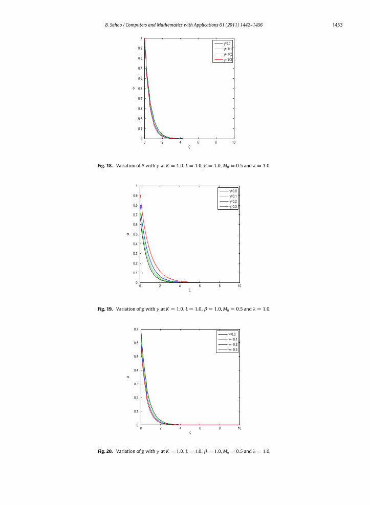
Variations of the temperature profiles for the PST and PHF caseswith the non-dimensional source and sink parameters areshown in Figs. 17–20. Fig. 17 shows the thermal boundary layer thickness increasewith an increase in the source parameter,whereas the sink has an opposite effect on the thermal boundary layer thickness as is clear from Fig. 18. Figs. 19 and 20 depictthat source and sink have similar effects on the thermal boundary layer for the PHF case.

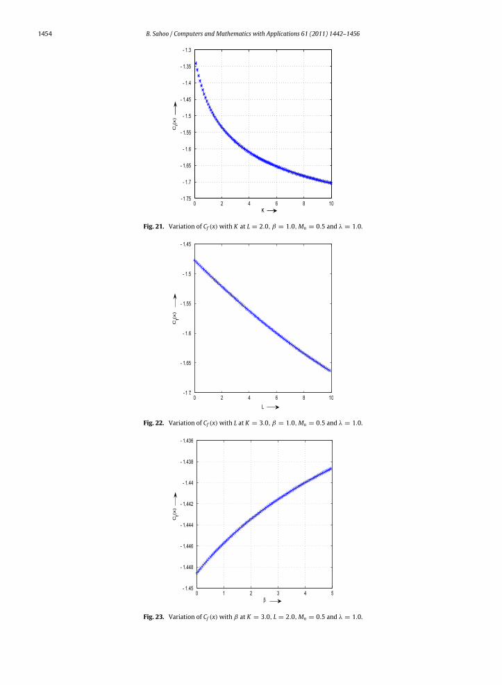
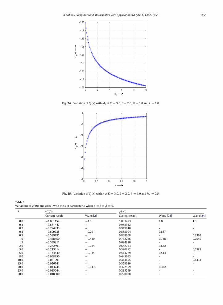
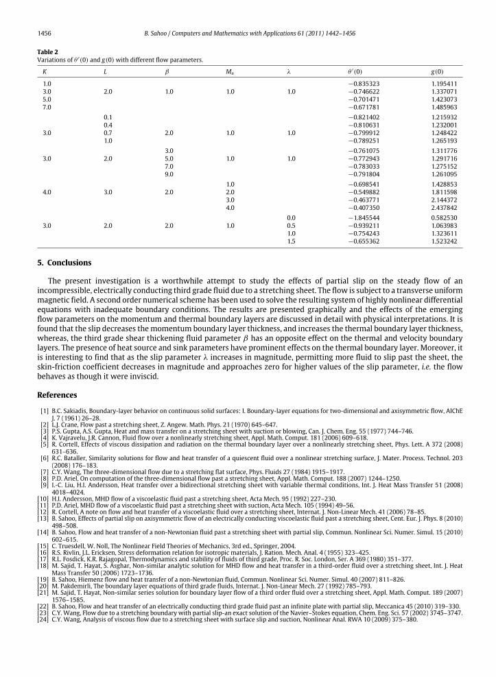
Figs. 21–25 elucidate the variations of the skin-friction coefficient Cf (x) with different flow parameters in presenceof slip with Rx = 1.0. Fig. 21 shows that the skin-friction coefficient is increased in magnitude with an increase in theviscoelasticity of the fluid. This prediction is of course undesirable from an industrial standpoint, because it translates into alarger driving force (or torque). The shear thickening parameter β decreases the magnitude of Cf (x), as is clear from Fig. 23.Fig. 24 shows that the magnitude of Cf (x) increases with an increase in the magnetic parameter Mn. Finally, the effects ofslip on Cf (x) is plotted in Fig. 25. It is apparent that the skin-friction coefficient decreases rapidly, and approaches zeroas the slip starts increasing. The values of the dimensionless surface temperature gradient θ ′(0) in the PST case, and thedimensionless surface temperature g(0) in the PHF case against different values of the flow parameters are tabulated inTable 2 for Pr = 2.0, Ec = 0.05 and constant value of γ . The data reveals that, in presence of slip, the magnitude of heattransfer rate (|θ ′(0)|) from the surface of the sheet to the fluid decreases with an increase in K . On the other hand, |θ ′(0)|increases with an increase in β . The magnetic interaction parameterMn and the slip parameter λ substantially decrease theheat transfer rate from the sheet to the ambient fluid.

Fig. 2. Variation of ϕ′ with K at L = 2.0, β = 1.0, Mn = 0.5 and λ = 1.0.

1448 B. Sahoo / Computers and Mathematics with Applications 61 (2011) 1442–1456

Fig. 3. Variation of ϕ′ with L at K = 3.0, β = 1.0, Mn = 0.5 and λ = 1.0.

Fig. 4. Variation of ϕ′ with β at K = 3.0, L = 2.0, Mn = 0.5 and λ = 1.0.

Fig. 5. Variation of ϕ′ withMn at K = 3.0, L = 2.0, β = 1.0 and λ = 1.0.

B. Sahoo / Computers and Mathematics with Applications 61 (2011) 1442–1456 1449

Fig. 6. Variation of ϕ′ with λ at K = 3.0, L = 2.0, β = 1.0 andMn = 0.5.

Fig. 7. Variation of θ with K at L = 2.0, β = 1.0,Mn = 0.5 and λ = 1.0.

Fig. 8. Variation of θ with L at K = 3.0, β = 1.0,Mn = 0.5 and λ = 1.0.

1450 B. Sahoo / Computers and Mathematics with Applications 61 (2011) 1442–1456

Fig. 9. Variation of θ with β at K = 3.0, L = 2.0,Mn = 0.5 and λ = 1.0.

Fig. 10. Variation of θ withMn at K = 3.0, L = 2.0, β = 1.0 and λ = 1.0.

Fig. 11. Variation of θ with λ at K = 3.0, L = 2.0, β = 1.0 and Mn = 0.5.

B. Sahoo / Computers and Mathematics with Applications 61 (2011) 1442–1456 1451

Fig. 12. Variation of g with K at L = 2.0, β = 1.0,Mn = 0.5 and λ = 1.0.

Fig. 13. Variation of g with L at K = 3.0, β = 1.0,Mn = 0.5 and λ = 1.0.

Fig. 14. Variation of g with β at K = 3.0, L = 2.0,Mn = 0.5 and λ = 1.0.

1452 B. Sahoo / Computers and Mathematics with Applications 61 (2011) 1442–1456

Fig. 15. Variation of g withMn at K = 3.0, L = 2.0, β = 1.0 and λ = 1.0.

Fig. 16. Variation of g with λ at K = 3.0, L = 2.0, β = 1.0 and Mn = 0.5.

Fig. 17. Variation of θ with γ at K = 1.0, L = 1.0, β = 1.0, Mn = 0.5 and λ = 1.0.

B. Sahoo / Computers and Mathematics with Applications 61 (2011) 1442–1456 1453

Fig. 18. Variation of θ with γ at K = 1.0, L = 1.0, β = 1.0,Mn = 0.5 and λ = 1.0.

Fig. 19. Variation of g with γ at K = 1.0, L = 1.0, β = 1.0,Mn = 0.5 and λ = 1.0.

Fig. 20. Variation of g with γ at K = 1.0, L = 1.0, β = 1.0,Mn = 0.5 and λ = 1.0.

1454 B. Sahoo / Computers and Mathematics with Applications 61 (2011) 1442–1456

Fig. 21. Variation of Cf (x) with K at L = 2.0, β = 1.0,Mn = 0.5 and λ = 1.0.

Fig. 22. Variation of Cf (x) with L at K = 3.0, β = 1.0,Mn = 0.5 and λ = 1.0.

Fig. 23. Variation of Cf (x) with β at K = 3.0, L = 2.0,Mn = 0.5 and λ = 1.0.

B. Sahoo / Computers and Mathematics with Applications 61 (2011) 1442–1456 1455

Fig. 24. Variation of Cf (x) withMn at K = 3.0, L = 2.0, β = 1.0 and λ = 1.0.

Fig. 25. Variation of Cf (x) with λ at K = 3.0, L = 2.0, β = 1.0 and Mn = 0.5.

Table 1Variations of ϕ′′(0) and ϕ(∞) with the slip parameter λ when K = L = β = 0.

λ ϕ′′(0) ϕ(∞)

Current result Wang [23] Current result Wang [23] Wang [24]

0.0 −1.001154 −1.0 1.001483 1.0 1.00.1 −0.871447 – 0.955952 – –0.2 −0.774933 – 0.919010 – –0.3 −0.699738 −0.701 0.888004 0.887 –0.5 −0.589195 – 0.838008 – 0.83931.0 −0.428450 −0.430 0.752226 0.748 0.75491.5 −0.339811 – 0.694880 – –2.0 −0.282893 −0.284 0.652253 0.652 –3.0 −0.213314 – 0.590892 – 0.59825.0 −0.144430 −0.145 0.513769 0.514 –8.0 −0.098150 – 0.445063 – –

10.0 −0.081091 – 0.413655 – 0.433115.0 −0.056741 – 0.359080 – –20.0 −0.043748 −0.0438 0.322559 0.322 –25.0 −0.035644 – 0.295599 – –50.0 −0.018600 – 0.220038 – –

1456 B. Sahoo / Computers and Mathematics with Applications 61 (2011) 1442–1456

Table 2Variations of θ ′(0) and g(0) with different flow parameters.

K L β Mn λ θ ′(0) g(0)

1.0 −0.835323 1.1954113.0 2.0 1.0 1.0 1.0 −0.746622 1.3370715.0 −0.701471 1.4230737.0 −0.671781 1.485963

0.1 −0.821402 1.2159320.4 −0.810631 1.232001

3.0 0.7 2.0 1.0 1.0 −0.799912 1.2484221.0 −0.789251 1.265193

3.0 −0.761075 1.3117763.0 2.0 5.0 1.0 1.0 −0.772943 1.291716

7.0 −0.783033 1.2751529.0 −0.791804 1.261095

1.0 −0.698541 1.4288534.0 3.0 2.0 2.0 −0.549882 1.811598

3.0 −0.463771 2.1443724.0 −0.407350 2.437842

0.0 −1.845544 0.5825303.0 2.0 2.0 1.0 0.5 −0.939211 1.063983

1.0 −0.754243 1.3236111.5 −0.655362 1.523242

5. Conclusions

The present investigation is a worthwhile attempt to study the effects of partial slip on the steady flow of anincompressible, electrically conducting third grade fluid due to a stretching sheet. The flow is subject to a transverse uniformmagnetic field. A second order numerical scheme has been used to solve the resulting system of highly nonlinear differentialequations with inadequate boundary conditions. The results are presented graphically and the effects of the emergingflow parameters on the momentum and thermal boundary layers are discussed in detail with physical interpretations. It isfound that the slip decreases themomentum boundary layer thickness, and increases the thermal boundary layer thickness,whereas, the third grade shear thickening fluid parameter β has an opposite effect on the thermal and velocity boundarylayers. The presence of heat source and sink parameters have prominent effects on the thermal boundary layer. Moreover, itis interesting to find that as the slip parameter λ increases in magnitude, permitting more fluid to slip past the sheet, theskin-friction coefficient decreases in magnitude and approaches zero for higher values of the slip parameter, i.e. the flowbehaves as though it were inviscid.

References

[1] B.C. Sakiadis, Boundary-layer behavior on continuous solid surfaces: I. Boundary-layer equations for two-dimensional and axisymmetric flow, AIChEJ. 7 (1961) 26–28.

[2] L.J. Crane, Flow past a stretching sheet, Z. Angew. Math. Phys. 21 (1970) 645–647.[3] P.S. Gupta, A.S. Gupta, Heat and mass transfer on a stretching sheet with suction or blowing, Can. J. Chem. Eng. 55 (1977) 744–746.[4] K. Vajravelu, J.R. Cannon, Fluid flow over a nonlinearly stretching sheet, Appl. Math. Comput. 181 (2006) 609–618.[5] R. Cortell, Effects of viscous dissipation and radiation on the thermal boundary layer over a nonlinearly stretching sheet, Phys. Lett. A 372 (2008)

631–636.[6] R.C. Bataller, Similarity solutions for flow and heat transfer of a quiescent fluid over a nonlinear stretching surface, J. Mater. Process. Technol. 203

(2008) 176–183.[7] C.Y. Wang, The three-dimensional flow due to a stretching flat surface, Phys. Fluids 27 (1984) 1915–1917.[8] P.D. Ariel, On computation of the three-dimensional flow past a stretching sheet, Appl. Math. Comput. 188 (2007) 1244–1250.[9] I.-C. Liu, H.I. Andersson, Heat transfer over a bidirectional stretching sheet with variable thermal conditions, Int. J. Heat Mass Transfer 51 (2008)

4018–4024.[10] H.I. Andersson, MHD flow of a viscoelastic fluid past a stretching sheet, Acta Mech. 95 (1992) 227–230.[11] P.D. Ariel, MHD flow of a viscoelastic fluid past a stretching sheet with suction, Acta Mech. 105 (1994) 49–56.[12] R. Cortell, A note on flow and heat transfer of a viscoelastic fluid over a stretching sheet, Internat. J. Non-Linear Mech. 41 (2006) 78–85.[13] B. Sahoo, Effects of partial slip on axisymmetric flow of an electrically conducting viscoelastic fluid past a stretching sheet, Cent. Eur. J. Phys. 8 (2010)

498–508.[14] B. Sahoo, Flow and heat transfer of a non-Newtonian fluid past a stretching sheet with partial slip, Commun. Nonlinear Sci. Numer. Simul. 15 (2010)

602–615.[15] C. Truesdell, W. Noll, The Nonlinear Field Theories of Mechanics, 3rd ed., Springer, 2004.[16] R.S. Rivlin, J.L. Ericksen, Stress deformation relation for isotropic materials, J. Ration. Mech. Anal. 4 (1955) 323–425.[17] R.L. Fosdick, K.R. Rajagopal, Thermodynamics and stability of fluids of third grade, Proc. R. Soc. London, Ser. A 369 (1980) 351–377.[18] M. Sajid, T. Hayat, S. Asghar, Non-similar analytic solution for MHD flow and heat transfer in a third-order fluid over a stretching sheet, Int. J. Heat

Mass Transfer 50 (2006) 1723–1736.[19] B. Sahoo, Hiemenz flow and heat transfer of a non-Newtonian fluid, Commun. Nonlinear Sci. Numer. Simul. 40 (2007) 811–826.[20] M. Pakdemirli, The boundary layer equations of third grade fluids, Internat. J. Non-Linear Mech. 27 (1992) 785–793.[21] M. Sajid, T. Hayat, Non-similar series solution for boundary layer flow of a third order fluid over a stretching sheet, Appl. Math. Comput. 189 (2007)

1576–1585.[22] B. Sahoo, Flow and heat transfer of an electrically conducting third grade fluid past an infinite plate with partial slip, Meccanica 45 (2010) 319–330.[23] C.Y. Wang, Flow due to a stretching boundary with partial slip-an exact solution of the Navier–Stokes equation, Chem. Eng. Sci. 57 (2002) 3745–3747.[24] C.Y. Wang, Analysis of viscous flow due to a stretching sheet with surface slip and suction, Nonlinear Anal. RWA 10 (2009) 375–380.