Embed Size (px)
Citation preview

Effects of Sea Water Scrubbing
Final report
Marc Hufnagl, Research Centre Terramare, Schleusenstrasse 1, 26382 Wilhelmshaven, Germany
Prof. Dr. Gerd Liebezeit, Research Centre Terramare, Schleusenstrasse 1, 26382 Wilhelmshaven,Germany
Dr. Brigitte Behrends, School of Marine Science and Technology, University of Newcastle,Newcastle upon Tyne, NE1 7RU, UK
March 2005
This document, and more, is available for download at Martin's Marine Engineering Page - www.dieselduck.net

I
Index
1 PROJECT DESCRIPTION ............................ ................................ ................................ ............................. 1
2 SUMMARY ............................ ................................ ................................ ................................ ....................... 1
3 INTRODUCTION............................ ................................ ................................ ................................ ............. 1
4 MATERIAL AND METHODS FOR PRELIMINARY TRIALS............................ ................................ . 5
4.1 PH-BUFFER-CAPACITY OF NATURAL SEAWATER (M IX-TEST)............................ ................................ ....... 5
4.2 POLYCYCLIC AROMATIC HYDROCARBONS ............................ ................................ ................................ .. 6
5 MATERIAL AND METHODS: DETERMINATION OF ENVIRONMENTAL PARAMETERS AND
POLLUTANTS ............................ ................................ ................................ ................................ ....................... 10
5.1 SAMPLING POINTS, SAMPLING, TRANSPORT AND STORAGE ............................ ................................ ....... 10
5.1.1 Sampling in February and March ............................ ................................ ................................ ..... 105.1.2 Sampling in July, September and November ............................ ................................ ..................... 12
5.2 TEMPERATURE, PH, SALINITY, OXYGEN ............................ ................................ ................................ .... 14
5.3 METALS AND SULPHATE ............................ ................................ ................................ ............................ 15
5.4 POLYCYCLIC AROMATIC HYDROCARBONS (PAH)............................ ................................ ..................... 15
5.4.1 Calibration, determination of accuracy, Carry-over ............................ ................................ ........ 155.4.2 Extraction............................ ................................ ................................ ................................ .......... 205.4.3 Determination of the origin of PAHs ............................ ................................ ................................ 22
5.5 PLANKTON SAMPLES ............................ ................................ ................................ ................................ .. 23
6 MATERIAL AND METHODS: TOXICITY TESTS AND ACCUMULATION TEST....................... 24
6.1 LUMISTOX............................ ................................ ................................ ................................ .................. 24
6.2 BRINE SHRIMP TEST ............................ ................................ ................................ ................................ ... 24
6.3 ACCUMULATION TEST ............................ ................................ ................................ ................................ 25
6.3.1 Preparation and Performance............................ ................................ ................................ ........... 256.3.2 Analysis and extraction of the mussels ............................ ................................ .............................. 27
7 RESULTS OF PRELIMINARY TRIALS ............................ ................................ ................................ .... 29
7.1 PH-MIXTURES............................ ................................ ................................ ................................ ............ 29
7.1.1 Jade Bay, Wilhelmshaven, Germany ............................ ................................ ................................ . 297.1.2 Ems River, Papenburg, Germany............................ ................................ ................................ ...... 307.1.3 Odense, Denmark ............................ ................................ ................................ .............................. 307.1.4 Calais, France ............................ ................................ ................................ ................................ ... 317.1.5 Dover, England ............................ ................................ ................................ ................................ . 317.1.6 Comparison of all results (in equilibrium) ............................ ................................ ........................ 32
7.2 GC-MS VALIDATION ............................ ................................ ................................ ................................ . 34
7.3 PAH-EXTRACTION, VALIDATION OF METHOD ............................ ................................ .......................... 37
This document, and more, is available for download at Martin's Marine Engineering Page - www.dieselduck.net
II
8 RESULTS AND DISCUSSION OF ENVIRONMENTAL SAMPLINGS ............................ ................. 41
8.1 1STSAMPLING (FEBRUARY) ............................ ................................ ................................ ........................ 41
8.1.1 pH, Temperature, Salinity, Conductivity, Oxygen............................ ................................ ............. 418.1.2 Metals and Sulphate ............................ ................................ ................................ .......................... 428.1.3 Nutrients............................ ................................ ................................ ................................ ............ 438.1.4 Polycyclic Aromatic Hydrocarbons ............................ ................................ ................................ .. 44
8.2 2NDSAMPLING(MARCH)............................ ................................ ................................ ............................. 46
8.2.1 pH, Temperature, Salinity, Conductivity, Oxygen............................ ................................ ............. 468.2.2 Metals and Sulphate ............................ ................................ ................................ .......................... 488.2.3 Nutrients............................ ................................ ................................ ................................ ............ 518.2.4 Polycyclic Aromatic Hydrocarbons ............................ ................................ ................................ .. 52
8.3 3RD SAMPLING (JULY) ............................ ................................ ................................ ................................ . 58
8.3.1 pH, salinity and temperature............................ ................................ ................................ ............. 588.3.2 Nutrients............................ ................................ ................................ ................................ ............ 598.3.3 Polycyclic aromatic hydrocarbons............................ ................................ ................................ .... 61
8.4 4THSAMPLING (SEPTEMBER)............................ ................................ ................................ ....................... 66
8.4.1 pH, salinity and temperature............................ ................................ ................................ ............. 668.4.2 Nutrients............................ ................................ ................................ ................................ ............ 688.4.3 Metals and Sulphate ............................ ................................ ................................ .......................... 698.4.4 Polycyclic aromatic hydrocarbons............................ ................................ ................................ .... 70
8.5 5TH SAMPLING (NOVEMBER)............................ ................................ ................................ ....................... 75
8.5.1 pH, salinity and temperature............................ ................................ ................................ ............. 758.5.2 Metals and Sulphate ............................ ................................ ................................ .......................... 778.5.3 Nutrients............................ ................................ ................................ ................................ ............ 788.5.4 Polycyclic Aromatic Hydrocarbons ............................ ................................ ................................ .. 79
8.6 ANNUAL CIRCLE ............................ ................................ ................................ ................................ ........ 84
8.6.1 pH, salinity and temperature............................ ................................ ................................ ............. 848.6.2 Nitrate and sulphate ............................ ................................ ................................ .......................... 928.6.3 Polycyclic aromatic hydrocarbons............................ ................................ ................................ .... 938.6.4 Plankton samples ............................ ................................ ................................ ............................ 100
8.7 RESULTS OF MUSSEL ANALYSIS............................ ................................ ................................ ................ 102
8.8 RESULTS OF SEDIMENT ANALYSIS ............................ ................................ ................................ ............ 104
9 RESULTS AND DISCUSSION OF THE TOXICITY AND ACCUMULATION TESTS................. 109
9.1 LUMISTOX TEST ............................ ................................ ................................ ................................ ....... 109
9.2 BRINE SHRIMP TEST ............................ ................................ ................................ ................................ . 110
9.3 ACCUMULATION TEST ............................ ................................ ................................ .............................. 111
9.3.1 Mussel analyses: size, weight, condition index, fat content ............................ ............................ 1119.3.2 Mussel analyses: PAH content, accumulation, mortality ............................ ................................ 114
10 CONCLUSIONS ............................ ................................ ................................ ................................ ....... 122
REFERENCES............................ ................................ ................................ ................................ ...................... 126
REFERENCES WORLD WIDE WEB............................ ................................ ................................ ............... 129
This document, and more, is available for download at Martin's Marine Engineering Page - www.dieselduck.net
III
LIST OF FIGURES
FIG. 1: GEOGRAPHICAL POSITION OF DOVER AND CALAIS AND ROUTE OF THE “PRIDE OF KENT” INSIDE THE
CHANNEL ............................ ................................ ................................ ................................ ........................... 10
FIG. 2: DOVER HARBOUR SAMPLING POINTS (LEFT: SAMPLING ON 11.2.2004, RIGHT SAMPLING ON 24.3.2004)..... 11
FIG. 3: PHOTOS OF THE SEAWATER SCRUBBER SAMPLING POINTS INSIDE THE „PRIDE OF KENT“. L.: POINT 1
SEAWATER SCRUBBER INLET. M.L.: POINT 2 SEAWATER SCRUBBER OUTLET. M.R.: POINT 3 AND 5: OUTLET
AND INLET OF US FILTER, TOP OF CYCLONES. R.: POINT 4, 7 AND 8: TUBE GOING TO THE SETTLING TANK AND
TOP AND BOTTOM OF SAMPLING TANK. ............................ ................................ ................................ .............. 12
FIG. 4: VAN VEEN GRAB AND NISKIN LADLE FOR SEDIMENT AND WATER SAMPLES RESPECTIVELY........................ 22
FIG. 5: PICTURE OF ARTEMIA SALINA. THIS ORGANISM WAS USED FOR TOXICITY TESTS ............................ .............. 24
FIG. 6: PHOTOS OF THE EXPERIMENTAL DESIGN OF THE ACCUMULATION TEST. L.: ALL NINE AQUARIUMS WITH
AERATION PUMP. M.: CLOSE VIEW ON TO AN AQUARIUM WITH AERATION STONE AND MUSSELS PLACED ON
THE PVC NET............................. ................................ ................................ ................................ .................... 26
FIG. 7: LEFT: D IFFERENT AMOUNTS OF ACIDIFIED (PH 4) JADE BAY SEAWATER MIXED WITH NON-ACIDIFIED JADE
BAY SEAWATER. GIVEN IS THE DEVELOPMENT OF PH OVER TIME IN RELATION TO THE PERCENTAGE OF PH 4
WATER. RIGHT: SAME AS LEFT BUT ONLY 50 : 50 MIXING RATIO WITH DIFFERENT VOLUMES. ........................ 29
FIG. 8: LEFT: 50 : 50 MIXING RATIO OF ACIDIFIED (PH 4) JADE BAY AND NATURAL JADE BAY SEAWATER, WITH
DIFFERENT STIR BAR ROTATION SPEEDS. RIGHT: PH-VALUE IN EQUILIBRIUM IN DEPENDENCY OF MIXING RATIO
(% PH 4 SEAWATER) ............................ ................................ ................................ ................................ .......... 29
FIG. 9: LEFT: DIFFERENT AMOUNTS OF ACIDIFIED (PH 4) EMS RIVER WATER MIXED WITH NON ACIDIFIED EMS
RIVER WATER. G IVEN IS THE DEVELOPMENT OF PH OVER TIME. RIGHT: PH-VALUE IN EQUILIBRIUM AS
FUNCTION OF MIXING RATIO (% PH 4 SEAWATER) ............................ ................................ ............................. 30
FIG. 10: LEFT: D IFFERENT AMOUNTS OF ACIDIFIED (PH 4) ODENSE SEAWATER MIXED WITH NON ACIDIFIED
ODENSE SEAWATER. GIVEN IS THE DEVELOPMENT OF PH OVER TIME. RIGHT: PH-VALUE IN EQUILIBRIUM AS
FUNCTION OF MIXING RATIO (% PH 4 SEAWATER) ............................ ................................ ............................. 30
FIG. 11: LEFT: DIFFERENT AMOUNTS OF ACIDIFIED (PH 4) CALAIS SEAWATER MIXED WITH NON ACIDIFIED CALAIS
SEAWATER. GIVEN IS THE DEVELOPMENT OF PH OVER TIME. RIGHT: PH-VALUE IN EQUILIBRIUM AS FUNCTION
OF MIXING RATIO (% PH 4 SEAWATER) ............................ ................................ ................................ .............. 31
FIG. 12: LEFT: D IFFERENT AMOUNTS OF ACIDIFIED (PH 4) DOVER SEAWATER MIXED WITH NON ACIDIFIED DOVER
SEAWATER. GIVEN IS THE DEVELOPMENT OF PH. RIGHT: PH-VALUE IN EQUILIBRIUM AS FUNCTION OF MIXING
RATIO (% PH 4 SEAWATER)............................ ................................ ................................ ................................ 31
FIG. 13: LEFT: PH-VALUE IN EQUILIBRIUM OF MIXING RATIO (% PH 4 SEAWATER) FOR ALL PRELIMINARY PH
TRIALS. RIGHT:MEAN OF ALL TRIALS WITH STANDARD DEVIATION. ............................ ................................ . 32
FIG. 14: LEFT: MEAN PH VALUE (POINTS) AND STANDARD DEVIATION (ERROR BARS) IN EQUILIBRIUM OF MIXING
RATIO (% PH 4 SEAWATER) FOR ALL PRELIMINARY PH TRIALS. THE BLACK LINE SHOWS THE MODEL FITTED
TO THE POINTS AND THE RED LINE SHOWS THE 95 % CONFIDENCE INTERVAL OF THE MODEL. RIGHT: CHANGE
OF PH OVER PERCENTAGE ............................ ................................ ................................ ................................ .. 32
FIG. 15: RESULTS OF PRELIMINARY TRIALS FOR THE DETERMINATION OF THE RECOVERY RATES OF PAHS FROM
SEAWATER. ............................ ................................ ................................ ................................ ........................ 38
This document, and more, is available for download at Martin's Marine Engineering Page - www.dieselduck.net

IV
FIG. 16: RESULTS OF PRELIMINARY TRIALS FOR THE DETERMINATION OF RECOVERY RATES OF PAHS FROM
SEAWATER. ............................ ................................ ................................ ................................ ........................ 38
FIG. 17: RESULTS OF PRELIMINARY TRIALS FOR THE DETERMINATION OF RECOVERY RATES OF PAHS FROM
SEAWATER. ............................ ................................ ................................ ................................ ........................ 38
FIG. 18: RECOVERY RATES OF THE SOLUBLE PAHS FROM NATURAL SEAWATER WITH CHROMABOND SPE SORBENT
C18 EC AND ELUTION SOLVENT DCM. LEFT: CALAIS SEAWATER RIGHT: DOVER SEAWATER. ...................... 39
FIG. 19: FRACTIONATION OF PAHS BETWEEN DISSOLVED AND PARTICULATE FRACTION AFTER DIFFERENT
INCUBATION TIMES. ............................ ................................ ................................ ................................ ........... 40
FIG. 20: MEAN RECOVERY RATE AND STANDARD DEVIATION FOR EIGHT EXTRACTIONS OF DOVER SEAWATER AND
PARTICULATE FRACTION. ............................ ................................ ................................ ................................ ... 40
FIG. 21: THE AUXILIARY ENGINES AND SWS RUNNING AT THE 24.03.04 ............................ ................................ ... 46
FIG. 22: LEFT: COPPER CONCENTRATION [PPB] RIGHT: MANGANESE CONCENTRATION [PPB] DETERMINED FOR
ECOSILENCER INLET AND OUTLET SAMPLES TAKEN IN CALAIS, DOVER AND THE CHANNEL ON 23/24.03.2004
AND ON 11.02.2004. IAPSO: ATLANTIC WATER SALINITY STANDARD ............................ .............................. 49
FIG. 23: LEFT: ZINC CONCENTRATION [PPB] RIGHT: BARIUM CONCENTRATION [PPB] DETERMINED FOR
ECOSILENCER INLET AND OUTLET SAMPLES TAKEN IN CALAIS, DOVER AND THE CHANNEL ON 23/24.03.2004
AND ON 11.02.2004. IAPSO: ATLANTIC WATER SALINITY STANDARD ............................ .............................. 50
FIG. 24: LEFT: LITHIUM CONCENTRATION [PPB] RIGHT: STRONTIUM CONCENTRATION [PPB] DETERMINED FOR
ECOSILENCER INLET AND OUTLET SAMPLES TAKEN IN CALAIS, DOVER AND THE CHANNEL ON 23/24.03.2004
AND ON 11.02.2004. IAPSO: ATLANTIC WATER SALINITY STANDARD ............................ .............................. 50
FIG. 25: LEFT: CALCIUM CONCENTRATION [PPM] RIGHT: POTASSIUM CONCENTRATION [PPM] DETERMINED FOR
ECOSILENCER INLET AND OUTLET SAMPLES TAKEN IN CALAIS, DOVER AND THE CHANNEL ON 23/24.03.2004
AND ON 11.02.2004. IAPSO: ATLANTIC WATER SALINITY STANDARD ............................ .............................. 50
FIG. 26: LEFT: MAGNESIUM CONCENTRATION [PPB] RIGHT: SULPHATE CONCENTRATION [PPB] DETERMINED FOR
ECOSILENCER INLET AND OUTLET SAMPLES TAKEN IN CALAIS, DOVER AND THE CHANNEL ON 23/24.03.2004
AND ON 11.02.2004. IAPSO: ATLANTIC WATER SALINITY STANDARD ............................ .............................. 51
FIG. 27: PLOT OF ISOMERIC PHENANTHRENE/ANTHRACENE RATIOS AGAINST FLUORANTHENE/PYRENE RATIOS FOR
ALL SAMPLES TAKEN IN FEBRUARY AND MARCH ............................ ................................ .............................. 54
FIG. 28: PLOT OF ISOMERIC PHENANTHRENE/ANTHRACENE RATIOS AGAINST FLUORANTHENE/PYRENE RATIOS FOR
THE SEAWATER SCRUBBER SAMPLES TAKEN IN FEBRUARY AND MARCH. ............................ .......................... 55
FIG. 29: RESULTS OF THE PCA OF THE HARBOUR SAMPLES ............................ ................................ ....................... 57
FIG. 30: REGRESSION BETWEEN 1ST AND 2ND EXTRACTION LEFT: REGRESSION OF THE AMOUNT OF EXTRACTED
PARTICULATE MATERIAL [G] RIGHT: REGRESSION OF ALLPAHS [NG/L] (SUM PARTICULATE, DISSOLVED).... 62
FIG. 31: PLOT OF ISOMERIC PHENANTHRENE/ANTHRACENE RATIOS AGAINST FLUORANTHENE/PYRENE RATIOS FOR
ALL HARBOUR SAMPLES (LEFT) AND SEAWATER SCRUBBER SAMPLES (RIGHT) ............................ .................. 62
FIG. 32: RESULTS OF THE PCA OF THE HARBOUR SAMPLES ............................ ................................ ....................... 65
FIG. 33: REGRESSION BETWEEN 1ST AND 2ND EXTRACTION LEFT: REGRESSION BETWEEN THE AMOUNT OF
EXTRACTED PARTICULATE MATERIAL [G]. RIGHT: REGRESSION OF ALL DETERMINED PAH CONCENTRATIONS
[NG/L] (SUM, PARTICULATE, DISSOLVED) ............................ ................................ ................................ ........... 71
This document, and more, is available for download at Martin's Marine Engineering Page - www.dieselduck.net

V
FIG. 34: PLOT OF ISOMERIC PHENANTHRENE/ANTHRACENE RATIOS AGAINST FLUORANTHENE/PYRENE RATIOS FOR
ALL SAMPLES ............................ ................................ ................................ ................................ ..................... 73
FIG. 35: RESULTS OF THE PCA OF THE HARBOUR SAMPLES ............................ ................................ ....................... 74
FIG. 36: REGRESSION BETWEEN THE FIRST AND THE SECOND EXTRACTION. LEFT: FILTER WEIGHTS, RIGHT: PAH
CONCENTRATIONS............................. ................................ ................................ ................................ ............. 80
FIG. 37: PLOT OF ISOMERIC PHENANTHRENE/ANTHRACENE RATIOS AGAINST FLUORANTHENE/PYRENE RATIOS FOR
ALL SAMPLES ............................ ................................ ................................ ................................ ..................... 82
FIG. 38: RESULTS OF THE PCA OF THE HARBOUR SAMPLES ............................ ................................ ....................... 83
FIG. 39: SALINITY, TEMPERATURE, AND PH MEASURED AT POINT CAL 1 AND CAL 2 ............................ ................. 84
FIG. 40: SALINITY, TEMPERATURE, AND PH MEASURED AT POINT CAL 3 AND CAL 4 ............................ ................. 84
FIG. 41: SALINITY, TEMPERATURE, AND PH MEASURED AT POINT C5 AND C50 ............................ ......................... 85
FIG. 42: SALINITY, TEMPERATURE, AND PH MEASURED AT POINT C350 AND C750 ............................ ................... 85
FIG. 43: SALINITY, TEMPERATURE, AND PH MEASURED AT POINT DOV 1 AND DOV 2............................ ................ 86
FIG. 44: SALINITY, TEMPERATURE, AND PH MEASURED AT POINT DOV 3 AND DOV 4............................ ................ 86
FIG. 45: SALINITY, TEMPERATURE, AND PH MEASURED AT POINT D5 AND D50............................ ......................... 86
FIG. 46: SALINITY, TEMPERATURE, AND PH MEASURED AT POINT D350 AND D700............................ ................... 86
FIG. 47: SALINITY, TEMPERATURE, AND PH MEASURED AT POINT SD1 AND SD2 ............................ ...................... 88
FIG. 48: SALINITY, TEMPERATURE, AND PH MEASURED AT POINT SC1 AND SC2............................ ....................... 88
FIG. 49: SALINITY, TEMPERATURE, AND PH MEASURED AT POINT SCH1 AND SCH2 ............................ ................. 88
FIG. 50: TEMPERATURE DEPENDENCY OF PH. THE RED LINE SHOWS THE COURSE OF THE PH WHEN THE SAMPLE
WAS HEATED AND THE BLUE LINE SHOWS THE COURSE OF THE PH WHEN THE SAMPLE WAS COOLED DOWN
AGAIN. ............................ ................................ ................................ ................................ ............................... 88
FIG. 51: SALINITY, TEMPERATURE, AND PH MEASURED AT POINT SCH3 AND SCH5 ............................ ................. 89
FIG. 52: SALINITY, TEMPERATURE, AND PH MEASURED AT POINT SCH6 ............................ ................................ ... 89
FIG. 53: PH AND SALINITY IN THE HARBOUR OF DOVER. TRIANGLES REPRESENT THE NATURAL VARIABILITY
DURING ALL SAMPLINGS IN 2004. DIAMONDS REPRESENT THE VALUES OF THE TRANSECT SAMPLES. ............ 90
FIG. 54: PH AND SALINITY IN THE HARBOUR OF CALAIS. TRIANGLES REPRESENT THE NATURAL VARIABILITY
DURING ALL SAMPLINGS IN 2004. DIAMONDS REPRESENT THE TRANSECT VALUES. ............................ ........... 90
FIG. 55: PH IMPACT OF SWS EFFLUENTS ON THE RECEIVING HARBOUR WATER IN DOVER AND CALAIS AT THREE
SAMPLING (JULY, SEPT. AND NOV.) ............................ ................................ ................................ ................... 91
FIG. 56: TEMPERATURE [°C] IMPACT OF SWS EFFLUENTS ON THE RECEIVING HARBOUR WATER IN DOVER AND
CALAIS AT THREE SAMPLING (JULY, SEPT. AND NOV.) ............................ ................................ ...................... 91
FIG. 57: TEMPERATURES [°C] OF HARBOUR AND TRANSECT SAMPLES. ............................ ................................ ...... 91
FIG. 58: NITRATE CONCENTRATIONS [µMOL L- 1] OBSERVED DURING ALL SAMPLINGS. LEFT: PORT OF CALAIS.
RIGHT: PORT OF DOVER............................ ................................ ................................ ................................ ..... 92
FIG. 59: REGRESSION BETWEEN 1ST AND 2ND EXTRACTION LEFT: REGRESSION BETWEEN THE AMOUNT OF
EXTRACTED PARTICULATE MATERIAL [G]. RIGHT: REGRESSION OF ALL DETERMINED PAH CONCENTRATIONS
[NG/L] (SUM, PARTICULATE, DISSOLVED) ............................ ................................ ................................ ........... 97
FIG. 60: RESULTS OF THE PCA OF ALL HARBOUR SAMPLES TAKEN IN FEBRUARY (F), MARCH (M), JULY (J),
NOVEMBER (N) AND SEPTEMBER (S)............................ ................................ ................................ ................. 98
This document, and more, is available for download at Martin's Marine Engineering Page - www.dieselduck.net

VI
FIG. 61: PLOT OF ISOMERIC PHENANTHRENE/ANTHRACENE AND FLUORANTHENE/PYRENE RATIOS OF THE SEDIMENT
SAMPLES TAKEN IN DOVER AND CALAIS IN JULY, SEPTEMBER AND NOVEMBER. ............................ ............ 106
FIG. 62: PRINCIPAL COMPONENT ANALYSIS OF THE RELATIVE PAH CONCENTRATIONS (PERCENTAGES) OF THE
WATER, SEDIMENT AND MUSSEL SAMPLES TAKEN IN DOVER AND CALAIS IN JULY, SEPTEMBER AND
NOVEMBER. FIRST LETTER: W=WATER SAMPLE, S=SEDIMENT SAMPLE, M=MUSSEL SAMPLE (SMAL=SMALL
20-30MM, MEDI=MEDIUM 30-40MM, LARG=LARGE 40-50 MM). SECOND LETTER: J=JULY, S=SEPTEMBER,
N=NOVEMBER. LAST FOUR LETTERS: SAMPLING POINT............................. ................................ .................. 107
FIG. 63: RESULTS OF LUMISTOX TEST. SHOWN ARE THE DIFFERENCES BETWEEN SEAWATER SCRUBBER INLET AND
OUTLET WATER TAKEN DURING THE SAMPLING IN SEPTEMBER. THE PH SHOWN WAS THE PH OF THE OUTLET
SAMPLE ............................ ................................ ................................ ................................ ............................ 109
FIG. 64: MEAN PERCENTAGES OF SHELL, DRY AND WET TISSUE WEIGHT FOR ALL MUSSELS USED IN THE
ACCUMULATION TEST. LEFT: PERCENTAGES FOR EACH TEST. RIGHT: MEAN FOR ALL TESTS ........................ 112
FIG. 65: CORRELATION PLOTS. LEFT: WHOLE WET WEIGHT AGAINST LENGTH. RIGHT: SHELL WEIGHT AGAINST
LENGTH. IN BOTH CASES THE RED LINE SHOWS THE NONLINEAR MODEL AND THE BLACK LINES THE 95 %
CONFIDENCE INTERVAL............................ ................................ ................................ ................................ .... 113
FIG. 66: CORRELATION PLOTS : LEFT: WET TISSUE WEIGHT AGAINST LENGTH. MIDDLE: DRY TISSUE WEIGHT
AGAINST LENGTH. RIGHT: DRY TISSUE WEIGHT AGAINST WET TISSUE WEIGHT. IN BOTH CASES THE RED LINE
SHOWS THE NONLINEAR MODEL AND THE BLACK LINES THE 95 % CONFIDENCE INTERVAL.......................... 113
FIG. 67: LEFT: COMPARISON OF PAH CONCENTRATIONS DETERMINED IN THE STANDARD MUSSEL TISSUE AND THE
ORIGINAL CONCENTRATIONS. RIGHT: CORRELATION COEFFICIENTS, STEEPNESS AND SECTION OF THE
EXTERNAL REFERENCE LINES ............................ ................................ ................................ ........................... 115
FIG. 68: MEAN CONCENTRATIONS OF THE ADDED PAHS, DETERMINED FOR THE DIFFERENT ACCUMULATION TESTS.
............................ ................................ ................................ ................................ ................................ ........ 116
FIG. 69: MEAN CONCENTRATIONS OF THE PAHS WHICH WERE NOT ADDED DURING THE TEST, DETERMINED FOR
THE DIFFERENT ACCUMULATION TESTS............................. ................................ ................................ ........... 116
FIG. 70: CONCENTRATIONS OF PHENANTHRENE, ANTHRACENE, FLUORANTHENE, PYRENE AND CHRYSENE IN NG L-1
MEASURED IN THE AQUARIUMS OF THE CONTROLS, THE PARTICULATE AND THE DISSOLVED TEST ONE HOUR
AFTER A WATER EXCHANGE AND RIGHT BEFORE THE FOLLOWING WATER EXCHANGE (3 DAYS).
CONCENTRATIONS ARE SEPARATED INTO THE DISSOLVED AND THE PARTICULATE FRACTIONS.................... 118
This document, and more, is available for download at Martin's Marine Engineering Page - www.dieselduck.net

VII
List of tables
TABLE 1: COMPOSITIONS OF MIXTURES FOR PH-BUFFER-CAPACITY MIX TEST. (M IXTURES WRITTEN IN ITALICS
WERE NOT PERFORMED FOR EVERY TRIAL) ............................ ................................ ................................ .......... 5
TABLE2: PROPERTIES OF THE DIFFERENT RIVER- AND SEAWATER SAMPLES USED FOR THE PRELIMINARY TRIALS .. 5
TABLE3: SAMPLING POINTS IN DOVER 11.02.2004 AND 24.03.2004-05-28 ............................ .............................. 11
TABLE4: SAMPLING POINTS IN CALAIS ............................ ................................ ................................ ..................... 11
TABLE5: SAMPLING POINTS ON BOARD „PRIDE OF KENT“ ............................ ................................ ......................... 11
TABLE6: SAMPLING POINTS IN CALAIS FOR THE SAMPLINGS IN JULY, SEPTEMBER AND NOVEMBER .................... 13
TABLE7: SAMPLING POINTS IN DOVER FOR THE SAMPLINGS IN JULY, SEPTEMBER AND NOVEMBER..................... 13
TABLE8: EBB AND FLOW DATES FOR ALL SAMPLINGS (HTTP://WWW.MOBILEGEOGRAPHICS.COM) ........................ 13
TABLE9: COORDINATES OF SAMPLING POINTS AND TIME AND DATE FOR SAMPLINGS ............................ ............... 14
TABLE10: GROUPS OF PAHS DEFINED FOR GC-MS SIM-METHOD ............................ ................................ ........... 15
TABLE11: STRUCTURES AND MAJOR PHYSICAL PROPERTIES OF THE 16 EPA-PAHS ............................ ................. 18
TABLE12: CATEGORIZATION OF THE ACCUMULATION TESTS. ............................ ................................ ................... 25
TABLE 13: MEAN PAH COMPOSITION IN THE SEAWATER SCRUBBER OUTLET SAMPLES (MARCH AND JULY), PAH
CONCENTRATIONS IN THE ACETONE SOLUTION AND RESULTING PAH CONCENTRATION IN THE AQUARIUM .. 26
TABLE14: DATES FOR WATER EXCHANGE DURING THE ACCUMULATION TEST ............................ .......................... 27
TABLE15: VALUES OBTAINED BY FITTING EQU. 12 TO THE PH-VALUES ............................ ................................ .... 33
TABLE16: STANDARD DEVIATION OF THREE DIFFERENT STANDARD DILUTION SERIES. ............................ ............. 34
TABLE17: ACCURACY OF THE GC MS (INCLUDING INJSTD, INTEGRATION AND MEASUREMENT)........................ 35
TABLE 18: F-TEST FOR LINEARITY OF THE GC MS. SHOWN RESULTS WERE CALCULATED WITH ALL DILUTION
STEPS RANGING FROM 2,5 TO 1000 µG L-1 ............................ ................................ ................................ ........... 35
TABLE 19: F-TEST FOR LINEARITY OF THE GC MS. SHOWN RESULTS WERE CALCULATED WITH ALL DILUTION
STEPS RANGING FROM 2,5 TO 100 µG L-1............................ ................................ ................................ ............ 36
TABLE20: LIMIT OF DETECTION (LOD) FOR DETERMINED PAHS............................ ................................ .............. 36
TABLE 21: MEAN RECOVERY RATES AND STANDARD DEVIATION DETERMINED FOR PRELIMINARY TRIALS WITH
ARTIFICIAL SEAWATER............................. ................................ ................................ ................................ ...... 39
TABLE 22: AIR AND WATER TEMPERATURE [°C], SALINITY [PSU], PH VALUE AND OXYGEN [MG L-1] DURING
SAMPLING IN CALAIS HARBOUR ON 11.2.2004 ............................ ................................ ................................ ... 41
TABLE 23: WATER TEMPERATURE [°C], SALINITY [PSU] AND PH-VALUE DURING SAMPLING IN DOVER HARBOUR
ON 11.2.2004 ............................ ................................ ................................ ................................ ..................... 41
TABLE 24: CONCENTRATIONS OF THE INTERNATIONAL ASSOCIATION FOR PHYSICAL SCIENCE OF THE OCEAN
STANDARD FOR NATURAL ATLANTIC SEAWATER. ............................ ................................ .............................. 42
TABLE 25: SULPHATE, EARTH AND TRANSITION METALS DETERMINED FOR THE SAMPLES TAKEN ON 11.02.2004.
FIELDS SIGNED WITH”-“ SHOW CONCENTRATIONS BELOW DETECTION LIMIT............................. .................... 43
TABLE26: NUTRIENT CONCENTRATIONS DETERMINED FOR THE SAMPLES TAKEN ON 11.02.2004 ......................... 43
TABLE 27: REGRESSION OF SAMPLE POINTS (SAMPLING 11.2.04). COLOURS ARE ADDED FOR A BETTER
VISUALISATION. YELLOW HIGHLY CORRELATED, RED MODERATE OR LOW CORRELATION, DARK RED NO
SIGNIFICANT. CORRELATION. ............................ ................................ ................................ ............................. 45
This document, and more, is available for download at Martin's Marine Engineering Page - www.dieselduck.net

VIII
TABLE 28: REGRESSION OF COMPOUND CONCENTRATIONS DETERMINED FOR THE SAMPLES TAKEN ON 11.2.04.
COLOURS ARE ADDED FOR A BETTER VISUALISATION. YELLOW HIGHLY CORRELATED, RED MODERATE OR
LOW CORRELATION, DARK RED NO SIGNIFICANT CORRELATION. ............................ ................................ ........ 45
TABLE 29: AIR AND WATER TEMPERATURE [°C], SALINITY [PSU], PH VALUE AND OXYGEN [MG L-1] DURING
SAMPLING IN CALAIS HARBOUR ON 23.3.2004 ............................ ................................ ................................ ... 46
TABLE 30: AIR AND WATER TEMPERATURE [°C], SALINITY [PSU], PH VALUE AND OXYGEN [MG L-1] DURING
SAMPLING IN DOVER HARBOUR ON 24.3.2004 ............................ ................................ ................................ ... 47
TABLE 31: AIR AND WATER TEMPERATURE [°C], SALINITY [PSU], PH VALUE AND OXYGEN [MG L-1] DURING
SAMPLING IN DOVER HARBOUR ON 24.3.2004 ............................ ................................ ................................ ... 47
TABLE 32: SULPHATE, EARTH AND TRANSITION METAL CONCENTRATIONS DETERMINED FOR THE SAMPLES TAKEN
IN JULY ............................ ................................ ................................ ................................ .............................. 49
TABLE33: NUTRIENT CONCENTRATIONS DETERMINED FOR THE SAMPLES TAKEN ON 24.03.2004 ......................... 52
TABLE34: INDICES FOR THE DETERMINATION OF THE ORIGIN OF THE PAHS (SAMPLES 11.02.04) ........................ 53
TABLE35: INDICES FOR THE DETERMINATION OF THE ORIGIN OF THE PAHS (HARBOUR SAMPLES 24.03.04) ....... 53
TABLE 36: INDICES FOR THE DETERMINATION OF THE ORIGIN OF THE PAHS (HARBOUR ECOSILENCER SAMPLES
24.03.04) ............................ ................................ ................................ ................................ ........................... 54
TABLE 37: INDICES FOR THE DETERMINATION OF THE ORIGIN OF THE PAHS (CANNEL OF DOVER ECOSILENCER
SAMPLES 24.03.04)............................ ................................ ................................ ................................ ............ 54
TABLE 38: REGRESSION CHART FOR THE ANALYSIS OF THE SAMPLING POINTS (SAMPLING MARCH). COLOURS ARE
ADDED FOR A BETTER V ISUALISATION. YELLOW HIGHLY CORRELATED, ORANGE AND RED MODERATE OR LOW
CORRELATION, DARK RED NO SIGNIFICANT. CORRELATION............................. ................................ ............... 55
TABLE 39: REGRESSION OF COMPOUND CONCENTRATIONS DETERMINED FOR THE SAMPLES TAKEN ON 24.03.04.
COLOURS ARE ADDED FOR A BETTER VISUALISATION. YELLOW HIGHLY CORRELATED, RED MODERATE OR
LOW CORRELATION, DARK RED NO SIGNIFICANT. CORRELATION............................. ................................ ....... 56
TABLE40: FEATURE VECTOR FOR THE PCA OF THE HARBOUR SAMPLES............................ ................................ .... 57
TABLE 41: TEMPERATURE, SALINITY AND PH DATA MEASURED AT THE DIFFERENT SAMPLING POINTS IN CALAIS
HARBOUR ............................ ................................ ................................ ................................ ........................... 58
TABLE 42: TEMPERATURE, SALINITY AND PH DATA MEASURED AT THE DIFFERENT SAMPLING POINTS IN DOVER
HARBOUR ............................ ................................ ................................ ................................ ........................... 58
TABLE43: SEAWATER SCRUBBER TEMPERATURES, SALINITIES AND PH DATA............................ ........................... 59
TABLE 44: CHLOROPHYLL, SESTON AND NUTRIENT CONCENTRATIONS DETERMINED FOR THE SAMPLES TAKEN IN
JULY 2004............................ ................................ ................................ ................................ .......................... 60
TABLE45: QUOTIENT OF BENZ[A]ANTHRACENE AND CHRYSENE. ............................ ................................ .............. 63
TABLE46: REGRESSION OF PAH COMPONENTS, YELLOW SHOWS HIGH CORRELATION............................ .............. 63
TABLE 47: REGRESSION OF SAMPLING POINTS. COLOURS ARE ADDED FOR A BETTER VISUALISATION. YELLOW
HIGHLY CORRELATED, DARK RED NO SIGNIFICANT CORRELATION. ............................ ................................ .... 64
TABLE48: FEATURE VECTOR FOR THE PCA OF THE HARBOUR SAMPLES............................ ................................ .... 65
TABLE 49: TEMPERATURE, SALINITY AND PH DATA MEASURED AT THE DIFFERENT SAMPLING POINTS IN CALAIS
HARBOUR IN SEPTEMBER ............................ ................................ ................................ ................................ ... 66
This document, and more, is available for download at Martin's Marine Engineering Page - www.dieselduck.net

IX
TABLE 50: TEMPERATURE, SALINITY AND PH DATA MEASURED AT THE DIFFERENT SAMPLING POINTS IN DOVER
HARBOUR IN SEPTEMBER ............................ ................................ ................................ ................................ ... 66
TABLE 51: TEMPERATURE, SALINITY AND PH DATA MEASURED AT THE DIFFERENT SAMPLING POINTS IN THE
SEAWATER SCRUBBER IN SEPTEMBER ............................ ................................ ................................ ................ 67
TABLE 52: CHLOROPHYLL, SESTON AND NUTRIENT CONCENTRATIONS DETERMINED FOR THE SAMPLES TAKEN IN
SEPTEMBER 2004............................ ................................ ................................ ................................ ............... 68
TABLE53: SULPHATE, EARTH AND TRANSITION METALS DETERMINED FOR THE SAMPLES TAKEN IN SEPTEMBER . 69
TABLE 54: REGRESSION OF COMPOUNDS. COLOURS ARE ADDED FOR A BETTER VISUALISATION. YELLOW HIGHLY
CORRELATED, DARK RED NO SIGNIFICANT CORRELATION. ............................ ................................ ................. 72
TABLE 55: REGRESSION OF SAMPLING POINTS. COLOURS ARE ADDED FOR A BETTER VISUALISATION. YELLOW
HIGHLY CORRELATED, DARK RED NO SIGNIFICANT CORRELATION. ............................ ................................ .... 72
TABLE 56: THE QUOTIENT OF BENZ[A]ANTHRACENE TO CHRYSENE CAN BE USED AS MARKER FOR THE ORIGIN OF A
SAMPLE ............................ ................................ ................................ ................................ .............................. 73
TABLE57: FEATURE VECTOR FOR THE PCA OF THE HARBOUR SAMPLES............................ ................................ .... 74
TABLE 58: TEMPERATURE, SALINITY AND PH DATA MEASURED AT THE DIFFERENT SAMPLING POINTS IN CALAIS
HARBOUR IN NOVEMBER............................ ................................ ................................ ................................ .... 75
TABLE 59: TEMPERATURE, SALINITY AND PH DATA MEASURED AT THE DIFFERENT SAMPLING POINTS IN DOVER
HARBOUR IN NOVEMBER............................ ................................ ................................ ................................ .... 76
TABLE 60: TEMPERATURE, SALINITY AND PH DATA MEASURED AT THE DIFFERENT SAMPLING POINTS IN THE
SEAWATER SCRUBBER HARBOUR IN NOVEMBER............................ ................................ ................................ 76
TABLE61: SULPHATE, EARTH AND TRANSITION METALS DETERMINED FOR THE SAMPLES TAKEN IN NOVEMBER.. 77
TABLE 62: SESTON AND NUTRIENT CONCENTRATIONS DETERMINED FOR THE SAMPLES TAKEN IN NOVEMBER 2004
............................ ................................ ................................ ................................ ................................ .......... 78
TABLE 63: REGRESSION OF PAH COMPOUNDS. COLOURS ARE ADDED FOR A BETTER VISUALISATION. YELLOW
HIGHLY CORRELATED, DARK RED NO SIGNIFICANT CORRELATION. ............................ ................................ .... 81
TABLE 64: REGRESSION OF SAMPLING POINTS. COLOURS ARE ADDED FOR A BETTER VISUALISATION. YELLOW
HIGHLY CORRELATED, DARK RED NO SIGNIFICANT CORRELATION. ............................ ................................ .... 81
TABLE65: ISOMERIC RATIOS OF BENZ[A]ANTHRACENE AND CHRYSENE ............................ ................................ .... 81
TABLE66: FEATURE VECTOR FOR THE PCA OF THE HARBOUR SAMPLES............................ ................................ .... 83
TABLE 67: D IFFERENCES BETWEEN THE INLET AND OUTLET SAMPLES TAKEN FROM THE SEAWATER SCRUBBER
SYSTEM IN CALAIS, DOVER AND THE CHANNEL. LEFT: PH DIFFERENCE. RIGHT: TEMPERATURE DIFFERENCE87
TABLE68: COMPARISON OF SULPHATE INLET AND OUTLET CONCENTRATIONS [PPM]............................ ................ 92
TABLE 69: SUM OF ALL 16 EPA-PAHS (PARTICULATE AND DISSOLVED, EXCLUDING NAPHTHALENE)
CONCENTRATIONS IN NG L-1
FOR ALL SAMPLINGS (N.D. = NOT DETERMINED)............................. .................... 93
TABLE70: PAH CONCENTRATIONS IN NG L-1. LISTED ARE THE CONCENTRATIONS OF THE SINGLE PAH COMPOUNDS
IN ALL SAMPLES. CONCENTRATIONS ARE GIVEN AS DISSOLVED/PARTICULATE PAH. DASHES INDICATE
CONCENTRATIONS BELOW THE LIMIT OF DETECTION. (N.D. = NOT DETERMINED)............................ ............... 93
TABLE 71: SUM OF BBF, BGHIP, BKF, BAP, FLUA, INDE. CALCULATED AS CARBON WEIGHT (N.D. NOT
DETERMINED) ............................ ................................ ................................ ................................ .................... 95
This document, and more, is available for download at Martin's Marine Engineering Page - www.dieselduck.net

X
TABLE 72: PAH CONCENTRATIONS IN NG L-1 DETERMINED FOR THE SEAWATER SCRUBBER SAMPLES. L ISTED ARE
THE CONCENTRATIONS OF THE SINGLE PAH COMPOUNDS IN ALL SAMPLES. CONCENTRATIONS ARE GIVEN AS
DISSOLVED/PARTICULATE PAH. DASHES INDICATE CONCENTRATIONS BELOW THE LIMIT OF DETECTION. (N.D.
= NOT DETERMINED) ............................ ................................ ................................ ................................ .......... 95
TABLE 73: DIFFERENCES [NG L-1] BETWEEN INLET AND OUTLET SAMPLES TAKEN IN MARCH, JULY, SEPTEMBER
AND NOVEMBER IN DOVER, CALAIS AND THE CHANNEL. SHOWN ARE THE MEAN, THE STANDARD DEVIATION
AND THE MINIMUM AND MAXIMUM VALUES. ............................ ................................ ................................ ..... 96
TABLE 74: FEATURE VECTOR FOR THE PCA OF ALL HARBOUR SAMPLES TAKEN IN FEBRUARY, MARCH, JULY,
NOVEMBER AND SEPTEMBER............................ ................................ ................................ ............................. 98
TABLE75: RESULTS OF PLANKTON CELL COUNTING. CONCENTRATIONS ARE GIVEN IN CELLS PER ML................ 100
TABLE 76: DIN DIFFERENCES BETWEEN INLET AND OUTLET SAMPLES TAKEN IN DOVER, CALAIS AND THE
CHANNEL............................. ................................ ................................ ................................ ........................ 102
TABLE 77: PAH CONCENTRATIONS [NG G-1] MEASURED IN MUSSELS TAKEN FROM THE QUAY WALLS AT SAMPLING
POINT C0 AND BIO CONCENTRATIONFACTORS (BCF). ............................ ................................ ................... 102
TABLE 78: PAH CONCENTRATIONS DETERMINED FOR SEDIMENT SAMPLES TAKEN IN JULY, SEPTEMBER AND
NOVEMBER............................ ................................ ................................ ................................ ...................... 104
TABLE 79: PAH COMPOSITION OF THE SEDIMENT SAMPLES TAKEN IN CALAIS AND DOVER IN JULY, SEPTEMBER
AND NOVEMBER IN PERCENT. ............................ ................................ ................................ .......................... 105
TABLE 80: FEATURE VECTOR FOR THE PCA OF THE WATER, SEDIMENT AND MUSSEL SAMPLES TAKEN IN DOVER
AND CALAIS INJULY, SEPTEMBER AND NOVEMBER ............................ ................................ ........................ 107
TABLE81: RESULTS OF THE BRINE SHRIMP TEST PERFORMED WITH 24 H OLD JUVENILE ARTEMIA SALINA ............ 110
TABLE82: RESULTS OF THE BRINE SHRIMP TEST PERFORMED WITH 4 WEEKS OLD JUVENILE ARTEMIA SALINA ..... 110
TABLE 83: LENGTH [MM] OF ALL MUSSELS EMPLOYED FOR THE ACCUMULATION TEST. THE COLOURS SEPARATE
THE TABLE IN THE MAIN CLASSES USED FOR THE PAH DETERMINATION. THE FIRST CLASS SMALLER THAN 50
MM AND THE SECOND CLASS BETWEEN 50 MM AND 60 MM............................ ................................ .............. 112
TABLE84: RESULTS OF LINEAR AND NONLINEAR REGRESSION ............................ ................................ ................ 113
TABLE 85: PAH CONCENTRATIONS [NG G-1] DETERMINED FOR THE MUSSELS FROM THE ACCUMULATION TEST.
WRITTEN IN ITALICS ARE THOSE COMPOUNDS ADDED DAILY. EXT ARE THE MUSSELS TAKEN FROM THE
EXTERNAL BASIN, 02, 05 AND 08 ARE THE CONTROLS, 03, 06 AND 09 ARE THE MUSSELS FROM THE DISSOLVED
TEST AND 01, 04 AND 07 ARE THE MUSSELS FROM THE PARTICULATE TEST. ............................ .................... 115
TABLE 86: EXPECTED PAH CONCENTRATIONS IN THE MUSSELS IF ALL ADDED PAHS WOULD HAVE BEEN
ACCUMULATED ............................ ................................ ................................ ................................ ................ 116
TABLE87: PERCENTAGE OF ACCUMULATED PAHS, CALCULATED AS QUOTIENT OF EXPECTED AND OBSERVED PAH
CONCENTRATION IN THE MUSSELS. ............................ ................................ ................................ .................. 117
TABLE88: PH, SALINITY AND TEMPERATURE DETERMINED IN THE AQUARIUMS DURING THE TEST ..................... 119
TABLE 89: TOTAL PAH AMOUNTS [MG] THAT WILL BE THEORETICALLY INTRODUCED DURING ONE DAY INTO THE
PORTS OF DOVER AND CALAIS AND THEORETICAL CONCENTRATION INCREASE [PG L-1] ............................ .. 120
TABLE 90: MEAN ACCUMULATION RATE, TOTAL ACCUMULATION PER DAY AND YEAR AND RESULTING
CONTAMINATION AFTER ONE YEAR FOR A 20 MM MUSSEL. ............................ ................................ .............. 120
This document, and more, is available for download at Martin's Marine Engineering Page - www.dieselduck.net

XI
TABLE 91: MEAN SHELL INDEX AND FAT CONTENT DETERMINED FOR THE MUSSELS OF THE ACCUMULATION TEST
AND FOR THE MUSSELS TAKEN IN CALAIS ............................ ................................ ................................ ........ 121
This document, and more, is available for download at Martin's Marine Engineering Page - www.dieselduck.net

XII
Abbreviations
Anth Anthracene
BaA Benz[a]anthracene
Chry Chrysene
DCM Dichloromethane
DIN Dissolved inorganic nitrogen
DIN Deutsche Industrie Norm
DOM Dissolved organic material
DOP Dissolved organic phosphorus
EPA Environmental Protection Agency
Flu Fluoranthene
FMN Flavin mononucleotid
GC-FID Gas-Chromatography Flame Ionisation Detector
GC-MS Gas-Chromatography Mass Spectroscopy
IAPSO International Association for Physical Science of the Ocean
ICP-OES Inductively Coupled Plasma Optical Emission Spectroscopy
IDL Instrument Detection Limit
InjSTD Injection Standard
ISTD Internal Standard
LOD Limit of Detection
PAH Polycyclic Aromatic Hydrocarbon
Phe Phenanthrene
PIP Particulate inorganic phosphorus
PoK “Pride of Kent” the ferry on which the seawater scrubber is installed
POP particulate organic phosphorus
Pyr Pyrene
RDP Reactive dissolved phosphorus
SI Shell Index
SIM Single Ion Monitoring
SPE Solid Phase Extraction
SQU Squalane (used as Injection Standard)
SWS Seawater scrubber
TBrB 1,2,4,5-Tetrabromobenzene (used as Injection Standard)
TDP Total dissolved phosphorus
TCHL Total chlorophyll
TPP total particulate phosphorus
This document, and more, is available for download at Martin's Marine Engineering Page - www.dieselduck.net

1 Project description2 Summary
1
1 Project description
In May 2003 BP-Marine in co-operation with P&O Ferries built a flue gas desulphurisation system
prototype manufactured by DME Canada into a channel ferry (“Pride of Kent”), operating between
Dover (UK) and Calais (France). To fulfil the legal requirements of Marpol Annex VI this seawater
scrubber should remove mainly SO2 from the exhaust gases. In addition other harmful emissions and
noise should also be reduced. The analysis of the liquid effluents as well as their influence on the
marine environment, especially that of the ports, was carried out by Terramare Research Centre in
Wilhelmshaven, Germany.
2 Summary
Within this project the effects of a seawater scrubber onto the environment were analysed. During five
sampling campaigns in 2004 the main focus was laid on pH, nutrients, temperature, trace metals,
polycyclic aromatic hydrocarbons (PAH) and plankton. Additionally one accumulation and two toxicity
tests were performed. For the observation of a whole annual cycle, samples were taken in February,
March, July, September and November inside the harbours of Dover and Calais and on board the
“Pride of Kent” (PoK). Inside the ferry’s seawater scrubber system very low pH values and high PAH
concentrations, even in the outlet, were measured. Sulphate and nitrate concentrations were also
higher on board than in samples from the harbour environment. Metal contents, especially of iron and
vanadium, which were leached from the steel, could also be detected in high amounts inside the
system. A decrease of the pH inside the ports or close to the ferry was never observed. Only in one
case the temperature was slightly higher in front of the effluent outlet. Although PAH concentrations
were high in the effluent, no increased concentrations were observed inside the harbours or in front of
the ship. Significant contents of heavy metals or eutrophication effects were also not detected. In
summary, no negative influence of the scrubbing system on the port environments was observed.
This document, and more, is available for download at Martin's Marine Engineering Page - www.dieselduck.net

3 Introduction
1
3 Introduction
Marine diesel engines are among the most fuel-efficient combustion sources for moving goods
[Corbett and Koehler, 2003]. Nevertheless they also contribute significantly to air pollution (e.g.
Capaldo et al., 1999; Streets et al., 2000). In the past regulations have been passed which dealt
especially with the SO2 emissions from land based combustion sources. Examples for these are the
European Union Directives 1999/30/EC, 2001/81/EC and 1999/32/EC. But since there were no
sulphur limits for marine heavy fuel oils, these now contain a high amount of sulphur relative to other
fuels.
Burning of fuel gives rise to SO2 and SOx formation, which damages sensitive ecosystems and
buildings. In the marine boundary layer especially ships contribute to a high input [Capaldo et al.,
1999]. Another by-product of fossil fuel burning is the emission of NOx. In marine regions with high
traffic, ships may increase NOx levels significantly. Both, SOx and NOx and additionally soot particles
not only cause environmental damage but also health damage. NOx for example increases, as well as
volatile organic compounds, the formation of ground level ozone. If the O3 concentration is elevated
above national standard levels (US EPA: 0.12 ppm) it may cause lung and respiratory disorders.
Additionally some materials like rubber, nylon, plastic, dyes and paints might be damaged by ozone. A
study revealed that children from rural Ontario communities show a decrease in lung function and
higher susceptibility for bronchitis [Mac Phail et al.]. Also plants, e.g. agricultural crops and trees, are
negatively affected by increased ozone concentrations [WHO 1997].
SOx and also NOx are also responsible for the formation of acid rain. Acid rain describes a
phenomenon which has been known since the early 1970s and which has caused a number of
problems [Driscoll et al. 2001]. For example in soils cations like Mg2+ and Ca2+ are leached whereas
sulphur and nitrogen concentrations increase. Additionally the harmful dissolved inorganic Al3+
increases which influences the water uptake capacity of trees. Moreover tree mortality has risen
because calcium is leached from the needles of gymnosperms thereby increasing their susceptibility
to freezing injury. In lakes the acid neutralising capacity is still decreasing resulting in an increasing
acidification and aluminium contents resulting in a decreasing species diversity. Model calculations
show that only with a marked reduction in sulphur emissions a measurable chemical improvement of
the affected ecosystems is possible. In many areas, mainly close to the major shipping routes and
harbours, sulphur emissions from ships may equal natural sources. The European Environment
Agency estimates that shipborne contributions from international shipping in the North Sea and north-
east Atlantic Ocean to total European acidifying emissions may about double by 2010 as a result of
increasing marine traffic (Fig. 1, EEA, 2000).
This document, and more, is available for download at Martin's Marine Engineering Page - www.dieselduck.net

3 Introduction
2
Fig. 1 Estimates of shipborne contributions to total European NOx and SO2 emissions 1990 – 2010 (EEA,2000)
To regulate especially this anthropogenic impact of SOx, an international instrument on air pollution
from ships was developed by the Maritime Organisation in 1997: Marpol Annex VI. Marpol Annex VI
was ratified in May 2004 by 15 flag states representing at least 50 % of the gross tonnage of the world
merchant shipping. It will come into force in May 2005. Furthermore, it has to be taken into account
that the cost of limiting the sulphur content of marine bunker oils in the North and Baltic Seas to 1.5 %
(the maximum value accepted by MARPOL) has been estimated at about 87 million €per year.
Equivalent reductions in total emissions from landbased sources (such as power stations) would cost
about 1,150 million €per year.
Among other regulations, Marpol Annex VI will introduce a 4.5 % sulphur limit for marine fuels and a
1.5 % sulphur limit for marine fuels burned in the so-called SOx emission control areas. Burning of fuel
with higher sulphur content is only allowed when technologies are used which reduce the atmospheric
emissions from ships to less than 6 g kWh -1 (as SO2 mass). Fluegas desulphurisation processes like
for examples seawater scrubbing are one possible technology [Tokerud, 1989]. These systems are no
new technology but have been used world wide since 1930 in coal power plants located close to the
sea (cf. Behrends and Liebezeit, 2003). Their main task is to reduce the sulphur dioxide (SO2) and
other sulphur oxides (SO x) contents in the exhaust gases which are produced from burning high
sulphur content coal. Additionally nitrogen oxides (NOx) and particulates are removed partially from the
exhaust gas. The reduction and the theoretical effects of a seawater scrubber system are described in
detail in Behrends and Liebezeit [2003]. Thereafter SOx and NOx dissolve within the scrubber effluent
and form nitric, nitrous and sulphuric acids. These might, on one hand, reduce the pH of the receiving
waters and, on the other hand, might due to the input of nitrate lead to eutrophication.
Besides gaseous components soot is also formed, especially during incomplete combustion. This is
mainly made up of elemental carbon with the particular features of a large surface area and a
hydrophobic character. Nonpolar substances immediately adsorb onto these particles and are then
transported with the soot from the combustion source. Polycyclic aromatic hydrocarbons (PAHs
constitute a major group of these substances. While the low molecular weight PAHs such as
This document, and more, is available for download at Martin's Marine Engineering Page - www.dieselduck.net

3 Introduction
3
naphthalene (two rings) or phenanthrene and anthracene (three rings) are mainly found unbound in
the gaseous phase already a major fraction of the four-ring members like pyrene, chrysene and
benz[a]anthracene are bound to these carbon particles.
The formation of PAHs and a major part of all reactions that take place during combustion have been
presented by Duran et al. 2004. In addition to this pyrolytic formation there are several other PAH
sources such as petrogenic oil formation processes. In this case these compounds are created during
the slow maturation of organic material. With regard to the sources of PAHs there is a broad spectrum
of possibilities for them to enter the environment: industrial wastewater, street dust runoff discharges,
deposition of fossil fuel combustion particles, carbonized coal product spills, forest and grass fires,
volcanic particles, oil spills or natural oil seeps [Witt and Trost, 1999; Lake et al. 1979, Lee et al.
1981]. Usually PAHs are occurring in a complex mixture of isomers and alkylated isomers [Wise et al.,
1993]. Low molecular weight PAHs with two or three rings are present normally in dissolved form in
water or gaseous in atmosphere. The higher the molecular weight the more hydrophobic they behave
and the more they are bound to particles [Ahrens, Depree, 2004, Pleil et al., 2004, Doong and Lin,
2004]. Therefore highest PAH concentrations are to be found in sediments [Neff 1979; Pearlman et
al., 1984].
Taking all sources in consideration it is not surprising that PAHs have not only been detected in
sediments but also in the atmosphere, water and soils all over the world [Fung et al. 2004; Soclo et al.
2000; Potrykus et al. 2003, Prevedouros et al. 2003]. Because some of them are toxic [Bispo et al.
1999; El-Alawi et al., 2001], some inhibit plant growth [Sudhakar Babu et al. 2001, Marwood et al.
2001] and some are carcinogenic and mutagenic [ATSDR 1997] their distribution and behaviour in the
environment has been subject to several studies.
When PAHs are introduced into the environment several reactions may occur. Besides to the
described adsorption to particles and also dissolved organic material (DOM) [Sun et al., 2003],
photooxidation is one of the major reactions. In most cases these photooxidized forms are even more
toxic than the parent compounds [Sudhakar Babu et al., 2001; El Alawi et al., 2001; McConkey et al.,
1997; Ankley et al. 1994]. For example the photooxidized form of anthracene inhibits the
photosynthetic electron transport system [Huang et al., 1997]
Biological degradation, mainly due to microbial action [Weissenfels et al., 1992; Heitkamp and
Cerniglia 1989], is another important factor in alteration and reduction. In this case it has to be taken
into consideration, that degradation of combustion derived PAHs is expected to be slower for PAHs
from petrogenic origin [Yunker et al., 1996; Mc Groddy and Farrington, 1995; Gustafsson et al., 1997]:
In addition, the PAH concentrations [Yuan et al. 2001], the amount of total organic carbon [Hinga
2003; Webster et al., 2001] and the particle size [Schnelle-Kreis et al. 1999] seem to play a role in
removing and degradation of PAHs from or in the water.
Additionally it has to be taken into account that because of the different sources of these PAHs, they
show a distinct seasonal variability [Prevedouros et al., 2004] and also degradation might show
seasonality [Pohlman et al. 2002]. These changes concern mainly combustion-derived PAHs. During
This document, and more, is available for download at Martin's Marine Engineering Page - www.dieselduck.net

3 Introduction
4
wintertime when there is lot of wood and oil burning, environmental concentrations rise. In some
regions forest fires in summer might also influence the seasonality.
The determination of the origin of PAHs is normally performed by the aid of different indices [Soclo et
al., 2000; Potrykus et al., 2003, Lake et al., 1979; see below]. All in all about 600 PAH-structures
[NIST 1997] have been classified and 16 of them have been defined by the United States
Environmental Protection agency (US-EPA) to be environmentally relevant [US-EPA 610]. These are
also the most common and best examined PAHs in the literature.
During the present study the impact of a Seawater Srubber (SWS) to reduce atmospheric emissions
was examined. The ship which was equipped with this technology was the "Pride of Kent", a ferry
operating between the harbours of Dover and Calais. The main focus of the survey was the harbours
and the seawater within the system of the SWS. Five samplings were performed, one sampling while
the SWS was not in use (11.02.2004) and four when the SWS was partially in use (March, July,
September and November), which means that only the seawater scrubbers for the auxiliary engines
were working.
Because both ports are influenced by tidal currents, the pH and the salinity showed a high natural
variability. In front of the outlet of the seawater scrubber no decrease in pH could be detected, but
effluent water was about 0.4 to 1.8 pH units lower than the inflow and the water within the harbour. An
effect on temperature could only be determined during the sampling in July and September.
Determined metal concentrations inside the harbour were mostly within the range of the used Atlantic
water salinity standard. The comparison between the SWS-inlet and the SWS-outlet water did only
indicate a rise of the zinc concentration which might haven been an effect of the sampling. Inside the
system iron and vanadium were increased but most of it was amassed inside the settling tank.
Within the harbours a seasonal variability of PAHs was determined with generally higher
concentrations in the winter, early spring and late autumn. Comparing the seawater inlet and outlet
samples, PAH-concentrations in the outlet were about two orders of magnitude higher than in the inlet.
Sulphate and nitrate were only increased inside the seawater scrubber but not inside the ports. The
toxicity tests did not clearly reveal an increased toxicity.
This document, and more, is available for download at Martin's Marine Engineering Page - www.dieselduck.net

4. Material and Methods
5
4 Material and Methods
4.1 pH - buffer capacity of natural seawater
The aim of this test was to estimate the buffer capacity of seawater and the time necessary to reach
pH-equilibrium after acid addition. The results could aid to predict the influence of the Ecosilencer
impact.
Five different natural sea- and brackish water samples (Jade Bay, Wilhelmshaven, Germany; Ems
River, Papenburg, Germany; Odense harbour, Denmark; Dover harbour, England; Calais harbour,
France). The different seawater properties are listed in Table 1.
Table 1: Properties of the different river- and seawater samples used for the assays
origin salinity[ppt]
pH samplingtemperature[°C]
testtemperature[°C]
Nassau harbour, Jade Bay,Wilhelmshaven, Germany
30 8,0 3 22,5
Meyer Werft, Ems River,Papenburg, Germany
0,3 7,71 3,1 22,6
Lindoe, Odense, Denmark 21,4 7,97 3,4 20,1Calais harbour, France 18,3 7,81 7,3 22,4Dover harbour, England 34,3 7,86 7,4 22,4
500 mL seawater each were acidified with a mixture of HNO3 and H2SO4 (1 : 1.48, v:v) to a final pH of
4.0. The mixing ratio of 1 to 1.48 was chosen because of the expected composition of the SWS
Ecosilencer effluent (sulphur content in fuel = 3.5 % and four main engines and two generators
running at 85 % MCR). The pH-value of pH 4 was chosen because of the worst case estimated pH of
the SWS Ecosilencer and cooling water mixture effluent discharges. The acidified water was then
mixed with the untreated seawater in different combinations (Table 2).
Table 2: Compositions of mixtures for pH buffer capacity test. (Mixtures in italics were not performed for everyassay)
acidified seawater(pH 4) [mL]
natural seawater(about pH 8) [mL]
stirring speed[rpm]
50 450 250100 400 250150 350 250200 300 250250 250 250250 250 250300 200 250350 150 250400 100 250450 50 250250 250 01000 1000 250500 500 250250 250 1000
This document, and more, is available for download at Martin's Marine Engineering Page - www.dieselduck.net

4. Material and Methods
6
After mixing the natural and the acidified samples, the pH was measured in regular intervals until no
significant change in pH could be observed any more. Normally the test was stopped after three days.
The pH for the different fractions was plotted against time and the pH in equilibrium was plotted
against the percentage of pH 4 seawater in mixture and analysed.
4.2 Polycyclic Aromatic Hydrocarbons
Several tests were performed to establish the best method for the extraction of PAHs on the basis of
the highest recovery rate. In the past liquid-liquid extraction was the commonly used technique to
extract PAHs from aqueous solutions, but as this method is cumbersome, labour intensive, expensive
and not environment-friendly due to its large solvent consumption, a less expensive and easier
method was developed. Solid phase extraction (SPE) was considered to be the best method,
especially as this method is favourably reported in literature [Crozier et al., 2001; Titato and Lanças,
2000; Garcia-Falcon et al. 2004] and different applications are available [Agilent Technologies;
Macherey Nagel]. Therefore different Solid Phase Extraction sorbents, different sample preparations
and different solvents were tested. For a comparison of the results the traditional liquid-liquid
extraction (LLE) was also applied. In a series of assays the following topics were investigated:
influence of SPE-sorbent
influence of elution solvent
influence of acetone addition before extraction
recoveries for Dover and Calais waters
incubation time of internal standard mix (fractionation of particulate and soluble PAH fractions)
recovery rate in artificial seawater for liquid-liquid-extraction (LLE) with n-hexane
For statistical reliability at least 3 parallel experiments were performed for every test. In every
experiment 500 mL of the matrix were spiked with 1 mL of a 100 µg L-1 PAH mixture in acetone
(Sigma-Aldrich Chemie GmbH, Taufkirchen Germany) containing acenaphthylene, anthracene,
benzo(a)anthracene, benzo(b)fluoranthene, benzo(k )fluoranthene, benzo(g)perylene, benzo(a)pyrene,
chrysene, dibenzo(ah)anthracene, fluorene, indeno(1,2,3-cd)pyrene, phenanthrene and pyrene. The
final concentration was 200 ng PAH L-1. Additionally 1 mL of a 100 µl L-1 Internal PAH Standard Mix
solution in acetone was added (Dr. Ehrenstorfer GmbH, Augsburg, Germany) containing
acenaphthene-D10, chrysene-D12, perylene-D12 and phenanthrene-D10. The first three tests which
are mentioned above were performed in artificial seawater [RiPSUa et al. 1979] produced with
deionised water, the remaining tests with natural seawater.
The SPE-cartridges were conditioned with 5 mL Methanol and flushed with about 100 mL deionised
water. Thereafter 500 mL sample were aspirated slowly over the SPE sorbent. For extraction 2 + 3 mL
This document, and more, is available for download at Martin's Marine Engineering Page - www.dieselduck.net

4. Material and Methods
7
dichloromethane (DCM) were used. An aliquot of 1000 µL from the resulting 5 mL extract was
transferred into a 2 mL amber glass-vial and 100 µl of a 10 µg mL -1 TBrB were added as injection
standard (InjSTD). The aliquot was analysed by gas chromatography/mass spectrometry (GC-MS;
GC: HP 6890, MS: HP MSD 5973, Software: Chemstation G1701 CA) in Single Ion Monitoring (SIM;
see Table 10).
Recoveries were determined by calculating the ratio of the measured PAH concentration and the
concentration added to the matrix. The means and the standard deviations were calculated. In the
following part the different assays are described in detail.
1. Influence of SPE-sorbent
Three different SPE-sorbents were used, all manufactured by Macherey-Nagel GmbH & Co KG,
Düren, Germany.
Chromabond EASY: a bifunctional modified polystyrene divinylbenzene copolymer phase (specific
surface 650 - 700 m² g-1, particle size 80 µm, pore size 50 Ångstrom, pH-range 1-14).
Chromabond C18 ec: an octadecyl silica endcapped sorbent (base material silica, pore size 60 Å,
particle size 45 µm for C18 ec, 100 µm for C18 ec f (fast flow), specific surface 500 m2 g-1, pH
stability 2 - 8, endcapped, carbon content 14 %).
Chromabond C18 PAH: an octadecyl silica phase for PAH analysis (60 Å, particle size 45 µm,
specific surface 500 m² g -1, pH stability 2 - 8).
Experiments were performed using artificial seawater.
2. Influence of Elution Solvent
SPE-cartridges filled with Chromabond C18 ec were used for extraction, two different elution solvents
were tested:
dichloromethane
n-hexane
Experiments were performed using artificial seawater.
3. Influence of Acetone Addition before Extraction
The extraction was performed using Chromabond C18 ec and DCM as elution solvent. During these
assays three different amounts of acetone were added to the sample before extraction.
2 mL acetone (0.2 %)
5 mL acetone (1 %)
10 mL acetone (2 %)
This document, and more, is available for download at Martin's Marine Engineering Page - www.dieselduck.net

4. Material and Methods
8
The matrix was artificial seawater.
4. Recovery rates in Dover and Calais harbour waters
As natural seawater taken from Dover and Calais harbours was already contaminated with PAHs,
another recovery experiment than that described above had to be executed. In this case three
samples of 500 mL Dover (11.02.04, station 7) and Calais (11.02.04, station 2) seawater were filled
into round flasks and spiked with 1 mL of a 100 ng mL-1 standard and internal standard solution.
These samples were then extracted using SPE-C18 ec and DCM as elution solvent. Three additional
500 mL samples from each harbour were spiked only with the internal standard. The recoveries are
then calculated by difference (see eq. 1).
100
11
spike
CalInjST
BS
CalInjST
s
C
StPAPA
SlPAPA
RR (1)
PAs = peak area of spiked sample
PAInjSTD = peak area of Injection Standard
SlCal = slope of calibration line
PABS = peak area of unspiked blank sample
Cspike = concentration of PAH spike
6. Incubation of Internal Standard Mix (Fractionation of Particulate and Soluble Fractions)
For this experiment ten subsamples of 0.5 L each, taken from a 20 L sample (24.3.2004, station 6:
Dover, “Prince of Whales Pier”) were filled into 1 L amber glass bottles, acidified with 2.5 mL 50 % HCl
and mixed with 0.5 mL 3 % sodium thiosulphate. Additionally the samples were spiked with 1 mL of a
100 µg L-1 PAH-mix and an equally concentrated ISTD Mix, closed and fixed on an orbital shaker. Two
subsamples made up one group and were extracted after 1 h, 2 h, 4 h, 8 h and 16 h. Then the
recoveries and the percentages of the soluble and the particulate fraction were determined. This
protocol was also used for the determination of the method repeatability and for the calculation of the
accuracy of the method.
7. Liquid-Liquid-Extraction
As liquid-liquid-extraction (LLE) was for long time the standard method to extract PAH from water, this
test was performed as reference. For extraction 500 mL artificial seawater were spiked with 1 mL
100 µg L-1 PAH-Mix and 1 mL 100 µg L-1 ISTD, acidified with 2.5 mL HCl (50%) and filled into a 1 L
separation funnel. The PAHs were then extracted with n-hexane (20 mL, 10 mL, 10 mL). All extracts
This document, and more, is available for download at Martin's Marine Engineering Page - www.dieselduck.net

4. Material and Methods
9
were combined, reduced in a rotary evaporator to dryness, taken up in 1 mL DCM and, after addition
of InjSTD, analysed by GC MS.
This document, and more, is available for download at Martin's Marine Engineering Page - www.dieselduck.net

5. Material and Methods: Determination of environmental parameters and pollutants
10
5 Material and Methods: Determination of environmental
parameters and pollutants
5.1 Sampling points, Sampling, Transport and Storage
5.1.1 Sampling in February and March
Samples were taken at nine different station inside the harbours of Dover (Fig. 3 and Table 3) and
Calais and at two (11.2.04) and twelve (24.3.04) places, respectively, inside the engine room of the
“Pride of Kent” during her operation inside the harbours and on the shipping route between Dover and
Calais (Fig. 2).
Fig. 2: Geographical position of Dover and Calais and route of the “Pride of Kent” in the Channel
As the Ecosilencer was not operative during the first sampling on 11.2.2004, only two samples were
taken from the seawater scrubber system: one from the inlet and one from the outlet. The samples
shown in Fig. 3 (left) were also taken from the seawater inlet. While the ship was entering the
harbours of Dover and Calais, samples were taken from the inlet and outlet. In the Channel additional
samples were taken at the points listed in Table 5 after some time of operation at normal load.
For the first sampling cleaned 2 L polyethylene flasks were used and rinsed with sample water before
filling. For the second sampling, the PAH-samples were stored in 1 L amber glass bottles (baked out
at 250 °C for 24 h and rinsed with 5 % HCl). Each one was filled with 1 L of sample and after that 5 mL
50 % HCl and 1 mL 3 % sodium thiosulphate were added to deactivate free chlorine and to prevent
samples from microbial degradation. For nutrient and metal samples 1 L polyethylene flasks treated as
the other polyethylene flasks mentioned before were used.
This document, and more, is available for download at Martin's Marine Engineering Page - www.dieselduck.net
5. Material and Methods: Determination of environmental parameters and pollutants
11
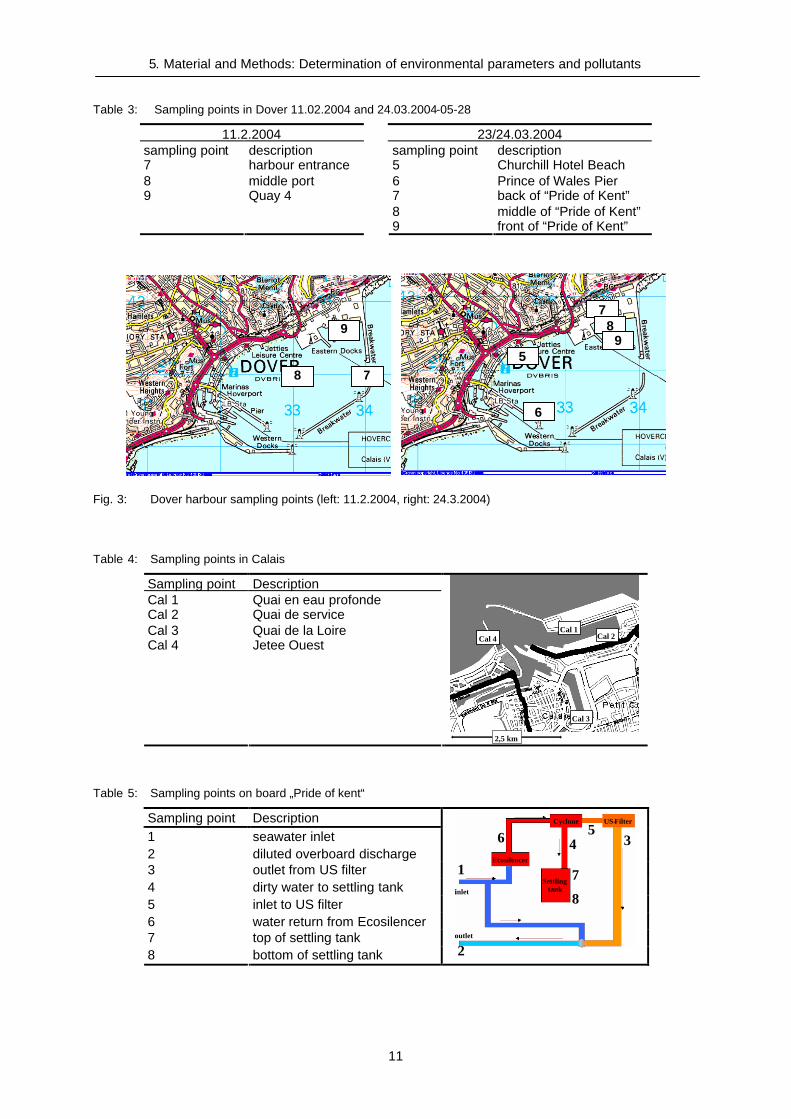
Table 3: Sampling points in Dover 11.02.2004 and 24.03.2004-05-28
11.2.2004 23/24.03.2004sampling point description sampling point description7 harbour entrance 5 Churchill Hotel Beach8 middle port 6 Prince of Wales Pier9 Quay 4 7 back of “Pride of Kent”
8 middle of “Pride of Kent”9 front of “Pride of Kent”
7
9
8
6
7
5
89
Fig. 3: Dover harbour sampling points (left: 11.2.2004, right: 24.3.2004)
Table 4: Sampling points in Calais
Sampling point DescriptionCal 1 Quai en eau profondeCal 2 Quai de serviceCal 3 Quai de la LoireCal 4 Jetee Ouest
Cal 1Cal 2
Cal 3
Cal 4
2,5 km
Table 5: Sampling points on board „Pride of kent“
Sampling point Description1 seawater inlet2 diluted overboard discharge3 outlet from US filter4 dirty water to settling tank5 inlet to US filter6 water return from Ecosilencer7 top of settling tank8 bottom of settling tank
inlet
outlet
Ecosilencer
Cyclone US-Filter
Settlingtankinlet
outlet
Ecosilencer
Cyclone US-Filter
Settlingtank
1
2
3456
7
8
This document, and more, is available for download at Martin's Marine Engineering Page - www.dieselduck.net

5. Material and Methods: Determination of environmental parameters and pollutants
12
Fig. 4: Photographs of the seawater scrubber sampling points inside the “Pride of Kent”. L.: Point 1 seawaterscrubber inlet. M.l.: Point 2 seawater scrubber outlet. M.r.: Point 3 and 5: outlet and inlet of US filter,top of cyclones. R.: Point 4, 7 and 8: tube going to the settling tank and top and bottom of samplingtank.
Inside the harbours 50 mL water samples for plankton determination were taken as well. These were
mixed with 10 drops “Lugol’s solution” (20 g KJ, 20 g J2, 200 mL deionised water, 20 mL acetic acid).
All bottles were transported in cooling boxes directly to the laboratory (max. 30 h), where they were
stored, with exception of the plankton samples, deep frozen at -18°C until further treatment or
extraction. The plankton samples were allowed to settle and the sample was analysed under an
inverted microscope.
5.1.2 Sampling in July, September and November
As for the samplings in July, September and November two small boats were available. The sampling
points changed and samples were also taken inside the harbours and within a transect from the outlet
of the seawater scrubber towards the entrance of the harbours. The sampling points, the description
and coordinates are given in Table 6, Table 7 and Table 9. In Table 9 the sampling times are also
given. The sampling points SD1, SD2, SC1, SC2 and SCH1 to SCH8 refer to the sampling points of
the seawater scrubber inside the “Pride of Kent”, where SD are the seawater scrubber samples taken
in Dover, SC are the samples taken in Calais and SCH are the samples taken during the Channel
crossing. Hih and low water times and flow for all samplings are shown in Table 8. As the “Pride of
Kent” did not berth at the predicted quay during the sampling in September the point C 0 was not
taken at the same place as C 5 but at a parallel quay.
This document, and more, is available for download at Martin's Marine Engineering Page - www.dieselduck.net

5. Material and Methods: Determination of environmental parameters and pollutants
13
Table 6: Sampling points in Calais for the samplings in July, September and November
Sampling point DescriptionCal 1 Quai en eau profondeCal 2 Quai de serviceCal 3 Quai de la LoireCal 4 Jetee OuestC 0 before arrival of “PoK”C 5 5 m from the outletC 50 50 m from the outletC 350 350 m from the outletC 700 700 m from the outlet
Cal 1Cal 2
Cal 3
Cal 4C 0C 5
C 50
C 350C 700
2,5 km
Table 7: Sampling points in Dover for the samplings in July, September and November
Sampling point DescriptionDov 1 eastern entranceDov 2 western entranceDov 3 middle portDov 4 close to Prince of Wales pierD 0 before arrival of “PoK”D 5 5 m from the outletD 50 50 m from the outletD 350 350 m from the outletD 700 700 m from the outlet
Table 8: High and low water times (http://www.mobilegeographics.com)
sampling port flow low water high waterFebruary Calais 11.2.04 3:44 11.2.04 10:45 11.2.04 16:07
Dover 11.2.04 15:37 11.2.04 22:37 12.2.04 2:56March Calais 23.3.04 14:21 23.3.04 21:14 24.3.04 2:36
Dover 24.3.04 0:04 24.3.04 7:04 24.3.04 12:23July Calais 13.7.04 10:50 13.7.04 17:35
Dover 13.7.04 9:09 13.7.04 16:11September Calais 8.9.04 8:06 8.9.04 14:32
Dover 7.9.04 4:29 7.9.04 11:07 7.9.04 17:01November Calais 17.11.04 3:27 17.11.04 10:37 17.11.04 15:52
Dover 16.11.04 12:33 16.11.04 19:48
This document, and more, is available for download at Martin's Marine Engineering Page - www.dieselduck.net

5. Material and Methods: Determination of environmental parameters and pollutants
14
Table 9: Coordinates of sampling points and time and date for samplings
Point coord. N coord. E July September NovemberCal 1 50° 58.161' 1° 51.491' 13.7.04 08:40 8.9.04 8:50 17.11.04 10:30Cal 2 50° 58.180' 1° 52.042' 13.7.04 09:00 8.9.04 9:05 17.11.04 10:00Cal 3 50° 57.385' 1° 51.562' 13.7.04 09:40 8.9.04 8:30 17.11.04 09:40Cal 4 50° 58.010 1° 50.582 13.7.04 10:00 8.9.04 8:15 17.11.04 09:30C 0 50° 58.052' 1° 51,382' - 8.9.04 11:15 17.11.04 11:00C 5 50° 58.044' 1° 50.927' 13.7.04 11:50 8.9.04 11:45 17.11.04 11:40C 50 50° 58.079' 1° 50.846' 13.7.04 12:00 8.9.04 12:00 17.11.04 11:50C 350 50° 58.153' 1° 50 634' 13.7.04 12:10 8.9.04 12:05 17.11.04 11:55C 700 50° 58.311' 1° 50.457' 13.7.04 12:30 8.9.04 12:10 17.11.04 12:00Dov 1 51° 07.109' 1° 20.459' 14.7.04 13:45 7.9.04 14:45 16.11.04 12:35Dov 2 51° 06.914' 1° 19.749' 14.7.04 13:50 7.9.04 15:05 16.11.04 13:00Dov 3 51° 07.100' 1° 19.854' 14.7.04 14:00 7.9.04 15:10 16.11.04 13:05Dov 4 51° 07.149' 1° 19.327' 14.7.04 14:05 7.9.04 15:17 16.11.04 13:10D 0 51° 07.584' 1° 20.406' 14.7.04 12:50 16.11.04 13:15D 5 51° 07.570' 1° 20.361' 14.7.04 13:05 7.9.04 14:10 16.11.04 13:20D 50 51° 07.526' 1° 20.387' 14.7.04 13:15 7.9.04 14:25 16.11.04 13:30D 350 51° 07.411' 1° 20.500' 14.7.04 13:20 7.9.04 14:35 16.11.04 13:25D 700 51° 07.292' 1° 20.589' 14.7.04 13:30 7.9.04 14:40 16.11.04 13:35SD1 - - 14.7.04 18:00 7.9.04 19:30 16.11.04 18:15SD2 - - 14.7.04 18:00 7.9.04 19:30 16.11.04 18:15SCH1 - - 14.7.04 18:30 7.9.04 20:00 16.11.04 18:50SCH2 - - 14.7.04 18:30 7.9.04 20:00 16.11.04 18:50SCH3 - - 14.7.04 18:55 7.9.04 20:10 16.11.04 18:50SCH4 - - - 7.9.04 20:10 16.11.04 18:55SCH5 - - 14.7.04 19:10 7.9.04 20:15 16.11.04 18:00SCH6 - - 14.7.04 19:15 7.9.04 20:15 16.11.04 18:55SCH7 - 7.9.04 20:20 -SCH8 - - - 16.11.04 19:00SC1 - - 14.7.04 19:25 7.9.04 20:55 16.11.04 19:40SC2 - - 14.7.04 19:25 7.9.04 20:55 16.11.04 19:40
5.2 Temperature, pH, Salinity, Oxygen
pH-values were measured directly after sampling using a pH-Meter (WTW pH 320/WTW-SenTix 81)
calibrated with two different buffer solutions (pH 7.00 and pH 4.01, Mettler-Toledo GmbH, Analytical,
Schwerzenbach, Switzerland). Salinity, conductivity and temperature were determined electronically
(WTW Cond 315i, Weilheim, Germany) as well.
Oxygen during the first sampling was determined by using a Winkler titration Kit (Merck, Germany).
During the second sampling (24.3.04) an oxygen electrode was used (Hach LDO HQ 10, range 0-
20 mg L-1, Düsseldorf, Germany).
This document, and more, is available for download at Martin's Marine Engineering Page - www.dieselduck.net

5. Material and Methods: Determination of environmental parameters and pollutants
15
5.3 Metals and sulphate
Metals were determined using Inductively Coupled Plasma Optical Emission Spectroscopy (ICP-
OES). Pre-treatment included acidification (5 % HNO3) and filtration (Syrfil Mixed Cellulose Ester
Filter, 25mm, 0.22 µm MF, Whatman, Maidstone, England; Norm Jet syringe, Tuttlingen, Germany).
For determination mainly elements which are included in the ships processes were chosen. These
include the transition metals vanadium, chromium, manganese, iron, cobalt, nickel, copper zinc and
molybdenum. Additionally the earth metals barium, lithium, strontium, calcium, potassium, magnesium
and the sulphate contents were measured. All samples were analysed by the working group “Inorganic
Geochemistry” at the Institute for Chemistry and Biology of the Sea (ICBM) at Oldenburg University,
Germany.
5.4 Polycyclic Aromatic Hydrocarbons (PAH)
5.4.1 Calibration, determination of accuracy, Carry-over
As the 16 EPA PAHs are the most widespread and commonly determined PAHs, these compounds
were also chosen for determination during this work. A composition of the names, synonyms and
major physical properties is shown in Table 11.
Table 10: Groups of PAHs defined for GC-MS SIM-method
group Ret. time Compound MS mass
1 - naphthalene 12812.52 acenaphthylene 15213.06 acenaphthene 154
222 12.96 acenaphtene-D10 164
14.80 fluorene 16633 17.14 1,2,4,5-tetrabromobenzene 393.7
18,11 phenanthrene-D10 19018.16 phenanthrene 178
444 18.32 anthracene 178
22.49 fluoranthene 20223.19 pyrene 20227.41 benzo[a]anthracene 22827.52 chrysene-D12 240
55555 27.96 chrysene 228
benzo[b]fluoranthene 25231.16 benzo[k]fluoranthene 25232.10 benzo[a]pyrene 252
6666 32.33 perylene 264
35.23 dibenz[a,h]anthracene 27835.37 indeno (1,2,3,c,d) pyrene 276
777 36.07 benzo[ghi]perylene 276
Calibration was performed by diluting a 500 mg L-1 PAH Mix (Sigma-Aldrich Chemie GmbH,
Taufkirchen Germany) to concentrations in a range from 1 to 1000 ng mL-1 three times. From every
dilution of the standard 1 mL was filled into an amber glass GC-vial and 50 µL of a 10 µg mL -1 of
This document, and more, is available for download at Martin's Marine Engineering Page - www.dieselduck.net

5. Material and Methods: Determination of environmental parameters and pollutants
16
1,2,4,5-tetrabromobenzene (TBrB) and 50 µL of a 10 µg mL-1 squalane solution were added as
injection standards (InjSTD). For the samples that have been taken during the fourth, fifth and sixth
sampling squalane was not used as injection standard. The calibration standards were prepared for
each chromatographic run and measured randomLy distributed over each analysis sequence. For
linear regression between concentrations and peak areas in relation to InjSTD the statistic program
Systat 8.0 was used (command file see appendix).
For determination of the linear range of the GC, a calibration series using nine concentrations in the
range from 2.5 ng mL-1 to 1000 ng mL-1 was analysed. The linearity was then determined by linear and
nonlinear regression of the calibration series with the nine different dilution steps. For linear regression
the function
bxay (2)
and for nonlinear regression the function
²xcxbay (3)
were fitted to the data. With these the value y could be calculated, which in the best case should be
the same value as the concentration y of the standard. In the next step the residual-standard-deviation
was calculated according to
N
iiilineary yy
Ns
1
2_ ˆ
21
(4)
N
iiinonlineary yy
Ns
1
2_ ˆ
31
(5)
where N is the number of dilution steps, y the employed concentration and y the concentration
calculated with the linear and nonlinear functions, respectively. From these values the difference DS²
can be calculated according to
2_
2_ 32² nonlinearylineary sNsNDS (6)
With this value the examination variable EV as
2_
²
nonlinearysDS
EV (7)
was determined and compared to F (P=099%, f1 = 1, f2 = N-3) from a F-table. If EV was smaller or
equal F the nonlinear function was not significantly better than the linear function. If this was not the
case, the highest concentration was taken out of the calculation, a new function was calculated and
EV was calculated again.
This document, and more, is available for download at Martin's Marine Engineering Page - www.dieselduck.net

5. Material and Methods: Determination of environmental parameters and pollutants
17
Accuracy of the GC was determined by measuring the 25 ng mL-1 and 500 ng mL-1 concentrations
eight times. To check for carry over, solvent blanks (DCM) were analysed distributed randomLy over
the chromatographic run.
The limit of detection (LOD) was determined as three times the standard deviation (IUPAC criterion) of
the 25 ng mL -1 concentration.
These tests were performed for the analyses with the split splitless injector and also for the samples
analysed with the cold injections system.
This document, and more, is available for download at Martin's Marine Engineering Page - www.dieselduck.net

5. Material and Methods: Determination of environmental parameters and pollutants
18
Table 11: Structures and major physical properties of the 16 EPA-PAHs
PAHs
EPAName and Synonyms Form. CAS Log KOW
(Exp./Calc.)[1]
Tboil
[°C][2]
Tfus
[°C][2]
Density[g cm-3]at 20°C [3]
Vapourpressure[Pa] [4]
Solub.H2O[mg/l] [4]
Molec.weight
Risk phrases Safetyphrases
hazardsymbol
naphthalene C10H8 91-20-3 3,33 / 3,17 217,0 80,2 - 1.0x10² 31 128,17 20,21, 22,36,37,38, 43,45
16,26, 36,37,39,45
Tacenaphthylene1,2-dihydroacenaphthylene1,8-dihydroacenapthalin1,8-ethylenenapthalene1,2-dihydroacenapththylene
C12H8 208-96-8 3,94 / 3,94 280,2 89,6 -93,4
- 9.0x10⁻¹ 16 152,19 22, 36, 37, 38 26, 36, 37, 39
Xn
acenaphthene,cyclopenta[d,e]naphthaleneparanaphthalene
C12H10 83-32-9 3,92 / 4,15 279,2 94 1.225 3.0x10⁻¹ 3.8 154,21 36, 37, 38 26, 36Xi
fluoreneortho-biphenylene methanediphenylenemethane2,2-methylene biphenyl2.3-benzidene
C13H10 86-73-7 4,18 / 4,02 294,2 -298,2
115 - 9.0x10⁻² 1.9 166,22 - -
Xn
anthraceneanthracingreen oil
C14H10 120-12-7 4,46 / 4,35 340 217 - 1.0x10⁻³ 0.045 178,2320, 21, 22,36, 37, 38,42,43
26, 36
Xn
phenanthrenephenantrin C14H10 85-01-8 4,45 / 4,35
328,15 -340,15 99
0.980at 4 °C 2.0x10⁻² 1.1 178,23
20, 21, 22,36, 37, 38, 40
26, 27, 36, 37,39, 45
Xn
fluoranthene1.2-[1,8-Naphthylene]-benzene1.2-benzacenaphthene1.2-[1.8- naphthalenediyl]benzenebenzo[j,k]fluorene
C16H10 206-44-0 5,16 / 4,93 - 108 -113
- 1.2x10⁻³ 0.26 202,25 22, 36, 37,38, 40
-
Xn
pyrenebenzo[d,e,f]phenanthrene8-pyrene
C16H10 129-00-0 4,88 / 4,93 - 151 1.271at 23 °C
6.0x10⁻⁴ 0.13 202,25 26, 36, 37, 38 -
Xn
benzo[a ]anthraceneBA;benz[a]anthracene1,2-benzanthracenebenzo[b]phenanthrene2,3-phenanthrene2,3-benzophenanthrenetetraphene,benzo[e]fluoranthene
C18H12 56-55-3 5,76 / 5,52 437,8 1591.274at 20 °C 2.8x10⁻⁵ 0.011 228,29 45, 50, 53 45, 53, 60, 61 T
N
This document, and more, is available for download at Martin's Marine Engineering Page - www.dieselduck.net

5. Material and Methods: Determination of environmental parameters and pollutants
19
chrysene1.2-benzophenanthrenebenzo[a]-phenanthrene1,2benzphenanthrenebenz[a]phenanthrene1,2,5,6-dibenzonaphthalene
C18H12 218-01-9 5,81 / 5,52 448,2 254,35 -258,4
- 5.7x10⁻⁷ 0.006 228,29 20, 21, 22,45, 46
3, 7, 9, 36, 37,39, 45
T
benzo[b]fluoranthene3,4-Benz[e]acephenanthrylene2,3-benzfluoranthene3,4-benzfluoranthene2,3benzofluoranthene3,4-benzofluoranthenebenzo[e]fluoranthene
C20H12 205-99-2 5,78 / 6,11 - - - - 0.0015 252,31 45, 50, 53 45, 53, 60, 61 T
Nbenzo[k ]fluoranthene8.9-benzfluoranthene8.9-benzofluoranthene11.12benzofluoranthene2,3,1.8-binaphthylenedibenzo[b,j,k]fluorine
C20H12 207-08-9 6,11 / 6,11 480 217 - 5.2x10⁻⁸ 0.0008 252,31 45 45, 53Xn
benzo[a ]pyrenebenzo[d,e,f]chrysene3-4 benzopyrene3,4-benzpyrenebenz[a]pyrene;BP
C20H12 50-32-8 6,13 / 6,11 495,2 1771.351
7.0x10⁻⁷ 0.0038 252,3145, 46, 50,53, 60, 61 45, 53, 60, 61
T
dibenz[a,h]anthraceneDB[a,h]ADBA1,2:5,6 dibenz[a ]anthracene
C22H14 53-70-3 -- / 6,70 524,2260,15 -271,2 1.282 3.7x10⁻¹⁰ 0.0006 278,35
indeno (1,2,3,c,d) pyreneindenopyreneIP;orthophenylenepyrene1,10-ortho-phenylene]pyrene1,10-[1,2-phenylene]pyrene2,3-ortho-phenylenepyrene
C22H12 193-39-5 6,63 / 6,70 -162 -163
- - 0.00019 276,33 - -
Xn
benzo[ghi]perylene1,12-benzoperylene C22H12 191-24-2 6,80* / 6,70 - 280 - 1.4x10⁻⁸ 0.00026 276,33 - 22, 24, 25 -
* Average from 3 reverences
[1] Heiden A.C., Hoffmann A., Kolahgar, B., (2001), Comparison of the Sensitivity of Solid Phase MicroExtraction (SPME) and Stir Bar Sorptive Extraction (SBSE) for the Dertermination of PolycyclicAromatic Hydrocarbons (PAHs) in Water and Soil Samples, Gerstel AppNote 8/2001, http://www.gerstelus.com/appnotes/new/Gerstel%202001/an-2001-08.pdf
[2] NIST Chemistry WebBook, http://webbook.nist.gov/chemistry[3] Tox Probe; Ten Carcinogens in Toronto; benzo[a]pyrene and other polycyclic aromatic hydrocarbons, http://www.city.toronto.on.ca/health/pdf/cr_appendix_b_pah.pdf[4] Staffan Lundstedt; 2003, Analysis of PAHs and their transformation products in contaminated soil and remedial processes http://publications.uu.se/umu/fulltext/nbn_se_umu_diva-57.pdf
This document, and more, is available for download at Martin's Marine Engineering Page - www.dieselduck.net
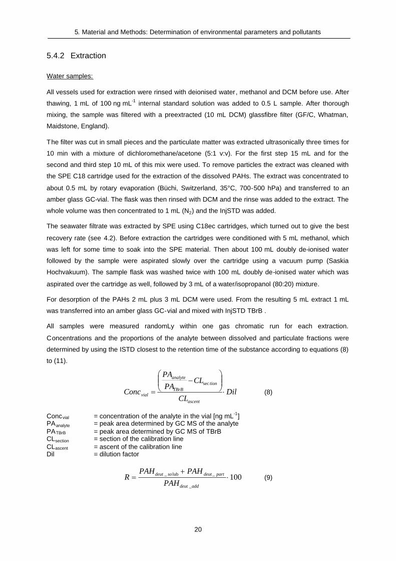
5. Material and Methods: Determination of environmental parameters and pollutants
20
5.4.2 Extraction
Water samples:
All vessels used for extraction were rinsed with deionised water, methanol and DCM before use. After
thawing, 1 mL of 100 ng mL-1 internal standard solution was added to 0.5 L sample. After thorough
mixing, the sample was filtered with a preextracted (10 mL DCM) glassfibre filter (GF/C, Whatman,
Maidstone, England).
The filter was cut in small pieces and the particulate matter was extracted ultrasonically three times for
10 min with a mixture of dichloromethane/acetone (5:1 v:v). For the first step 15 mL and for the
second and third step 10 mL of this mix were used. To remove particles the extract was cleaned with
the SPE C18 cartridge used for the extraction of the dissolved PAHs. The extract was concentrated to
about 0.5 mL by rotary evaporation (Büchi, Switzerland, 35°C, 700-500 hPa) and transferred to an
amber glass GC-vial. The flask was then rinsed with DCM and the rinse was added to the extract. The
whole volume was then concentrated to 1 mL (N2) and the InjSTD was added.
The seawater filtrate was extracted by SPE using C18ec cartridges, which turned out to give the best
recovery rate (see 4.2). Before extraction the cartridges were conditioned with 5 mL methanol, which
was left for some time to soak into the SPE material. Then about 100 mL doubly de-ionised water
followed by the sample were aspirated slowly over the cartridge using a vacuum pump (Saskia
Hochvakuum). The sample flask was washed twice with 100 mL doubly de-ionised water which was
aspirated over the cartridge as well, followed by 3 mL of a water/isopropanol (80:20) mixture.
For desorption of the PAHs 2 mL plus 3 mL DCM were used. From the resulting 5 mL extract 1 mL
was transferred into an amber glass GC-vial and mixed with InjSTD TBrB .
All samples were measured randomLy within one gas chromatic run for each extraction.
Concentrations and the proportions of the analyte between dissolved and particulate fractions were
determined by using the ISTD closest to the retention time of the substance according to equations (8)
to (11).
DilCL
CLPAPA
Concascent
tionTBrB
analyte
vial
sec
(8)
Concvial = concentration of the analyte in the vial [ng mL-1]PAanalyte = peak area determined by GC MS of the analytePATBrB = peak area determined by GC MS of TBrBCLsection = section of the calibration lineCLascent = ascent of the calibration lineDil = dilution factor
100_
_lub_
adddeut
partdeutsodeut
PAHPAHPAH
R (9)
This document, and more, is available for download at Martin's Marine Engineering Page - www.dieselduck.net

5. Material and Methods: Determination of environmental parameters and pollutants
21
100_
lub_lub
adddeut
sodeutso PAH
PAHF 100
_
_ adddeut
partdeutpart PAH
PAHF (10)
R = recovery rate [%]PAHdeut_solub = concentration of deuterated PAH determined for the soluble fraction [ng mL-1]PAHdeut_part = concentration of deuterated PAH determined for the particulate fraction [ng mL -1]PAHdeut_added = concentration of deuterated PAH added to the sample [ng mL-1]Fsolub = soluble fraction of the deuterated PAH [%]Fpart = particulate fraction of the deuterated PAH [%]
g
ngVV
FR
ConcConcConc Vial
sample
partvialsovialanalyte
10001_lub_
(11)
Concanalyte = concentration of the analyte in the water-sample [ng l-1]Concvial_solub = concentration of the soluble fraction of the analyte in the vial [ng mL-1]Concvial_part = concentration of the particulate fraction of the analyte in the vial [ng mL-1]F = soluble particulate fraction, respectivelyVsample = volume of the sample extractedVVial = volume of the extract in the vial
Sediment and Mussel samples
Mussel samples were only taken once in Calais during the sampling in November. Those mussels
were taken from a harbour stilt during ebb tide a point C0. About 60 mussels were collected randomly
and put into a freeze bag. The extraction and analysis of these mussels was performed in the same
way as described in section 6.3.2. To determine the accuracy of the extraction method a standard
reference mussel tissue was extracted. This was obtained from LGC Promochem (NIST-2977 Mussel
tissue - Organics and trace elements) and extracted twice at the same time as the mussels of the
accumulation test.
Sediments were taken in July at points C1, C5, C700 and D5, in September at points C5, C700 and
D700 and in November at points C5, C700 and D5. All samples were taken with a van Veen grab (Fig.
5), which takes abovut 150 cm² of the surface sediment, and were then transported to the lab in a
freeze bag. There they were deep frozen at -18 °C until extraction. Before the extraction the sediment
was freeze dried, coarse particles were removed and the remainder was ground in an agate ball mill
for 30 min at 180 rpm. From this fine, dried sediment 5 g were weight into a glass bottle and the
internal standard was added. The extraction was performed ultrasonically with 20 mL and two times
15 mL n-hexane for 15 min. As elemental sulphur negatively affects gas chromatographic analysis it
was removed with elemental copper. Oxides on the copper surface were removed by washing three
times with hydrochloric acid. The acid was removed by washing three times with deionised water and
the water was removed by washing three times with methanol. The methanol and eventually
remaining organic compounds bound to the copper surface were removed by washing three times with
DCM. About ten of these cleaned and activated copper filings were than added to the extracts and left
there for at least two hours. In those cases where the copper spans turned totally black (copper
sulphide) again about ten pieces were added and left in the extract for additional two hours. The
desulphurised extract was then filtered over NaSO4 to remove the copper spans and remaining water
This document, and more, is available for download at Martin's Marine Engineering Page - www.dieselduck.net

5. Material and Methods: Determination of environmental parameters and pollutants
22
from the extract and was then reduced to about 2 mL in a rotary evaporator. The clean-up was
performed on a silica column (5 g silica deactivated with 5 % H2O) and PAHs were eluted with 15 mL
n-hexane and with 20 mL of a n-hexane and DCM (5:1) mix. Both extracts were combined, reduced to
approximately 1 mL, transferred quantitatively into an amber glass 2 mL GC-vial and reduced to 1 mL
under N2. The injection standard was added and PAH concentrations were determined by GC-MS
Fig. 5: Van Veen grab and Niskin sampler for sediment and water samples respectively.
5.4.3 Determination of the origin of PAHs
PAHs in the environment might have different origins. Although there are some natural sources such
as oil seeps or some specific organisms, the main sources are anthropogenic. These include oil
released during normal ship operation or from accidents and products of incomplete combustion of
recent or fossil organic matter. To distinguish between these origins of a PAH mixture, some indices
have been developed in the past. The major aspect used is the thermodynamic stability. For example
phenanthrene (Phe) is thermodynamically more stable than its structural isomer anthracene (Anth).
The same is valid for fluoranthene (Flu) and pyrene (Pyr) pair. Concerning to these facts the Phe/Anth
ratio is higher in petrogenic (>10) than in pyrolytic pollution (<10). For Flu/Pyr a quotient of one was
determined. Thus a Flu/Pyr ration>1 points to a pyrolytic, while a Flu/Pyr rations <1 indicates a
petrogenic origin.
The chrysene (Chry) and benzo[a]anthracene (BaA) ratio is the basic for another index used. Chry
and BaA are derived from combustion processes at high temperatures with a Chry/BaA ratio <1. Also
an indicator for combustion derived PAHs is a higher abundance of four-, five- and six-ring PAHs in
comparison to the two- and three-ring PAHs, prominent in petrogenic sources.
This document, and more, is available for download at Martin's Marine Engineering Page - www.dieselduck.net

5. Material and Methods: Determination of environmental parameters and pollutants
23
An additional method which was used to determine the origin of the PAHs was principal component
analysis and the regression of samples and compounds resulting in different regression charts.
Principal component analyses (PCA) is a useful technique that has found application in fields such as
face recognition and image compression, and is a common technique for finding patterns in data of
high dimension. Therefore PCA has also been used to determine the origin of PAHs [Boehm et al.,
1997; Stella et al., 2002; Burns et al., 1997; Branislav et al., 2001]. The background of this method is
based in matrix algebra. In this case the analyses were performed by using a Matlab script, written by
M. Hufnagl (see Appendix). In the first step the data are standardised by substracting the mean. The
next step calculates the covariance matrix and then the eigenvector and the eigenvalues of this matrix.
In this case the feature vector, which is later used for the transformation of the data, was only made up
from the first two eigenvectors.
The regression of the compounds and the regression of the sampling points were performed using the
statistic program Systat. The source code is similar to that one shown in the Appendix. In the literature
this method was also used to determine PAH pollution sources [Adami et al. 2000].
5.5 Plankton samples
During the sampling in February and March plankton samples were taken in 50 mL bottles and
analysed qualitatively. During the samplings in July, September and November plankton samples
were taken from one, two and three meters water depth. From each depth one litre was taken with a
Niskin sampler (Fig. 5) and all three water samples were collected in a three litre PVC bottle. In the
laboratory the water was filtered over a 10 µm plankton net and 5 mL of the concentrated sample were
transferred to an Uttermöhl counting chamber where the cells were allowed to settle overnight. The
counting was performed with an inverted microscope. At 30 to 50 randomLy chosen points all plankton
cells within the given grid of the microscope were counted. The concentration of the counted cells
were then determined using the following equation
conc
S
ex VV
VfieldsAmlcells
105626.071.506/
where A is the amount of cells counted in the examined volume Vex. VS is the volume of the sample
and Vconc is the volume of the concentrated sample.
This document, and more, is available for download at Martin's Marine Engineering Page - www.dieselduck.net

6 Material and Methods: Toxicity and accumulation test
24
6 Material and Methods: Toxicity and accumulation tests
For these tests water was taken from the seawater scrubber inlet and outlet at point SCH1 and SCH2
during the fourth sampling which was performed in September. The samples were filled into Winkler -
bottles (250 mL) which disabled the gas exchange between the samples and the atmosphere. This
allows the examination of the samples in the laboratory at nearly unchanged conditions. The water
samples, five from the inlet and five form the outlet, where transported to the lab in cooling boxes and
then stored at 4 °C for two days before the toxicity tests were performed.
6.1 Lumistox
The bacterium used for this test was Vibrio fischeri. The enzymatically induced luminescence of this
bacterium is quantitatively easy to determine. The reaction that takes place is that the enzyme
luciferase oxidises chemical compounds like long chain aldehydes by aid of reduced FMN (flavin
mononucleotide) and O2 to the corresponding fatty acid. Within this reaction electrons are directly
transferred from the FMNH2 to the oxygen and energy is set free by emittance of light.
The test, produced by Dr. Bruno Lange GmbH, Berlin, is a standardized DIN (Deutsche Industrie
Norm) method used to analyze the contamination of water. The test was performed according to the
instructions given in the norm. From three different samples two parallels were screened resulting in
six values for the inlet and six values for the outlet. As blank a 2 % NaCl solution was analyzed.
6.2 Brine shrimp test
Another possibility to determine the toxicity of a substance is the mortality of organisms exposed to
that substance. Therefore during this test the mortality of juvenile and adult brine shrimp Artemia
salina (Fig. 6) was observed after placing it into subsamples of the inlet and outlet water.
Fig. 6: Picture of Artemia salina. This organism was used for toxicity tests
Due to the natural habitat of Artemia salina this organism is able to build long lasting eggs. Two days
before starting the test, about 200 mg of these eggs were placed into 1000 mL artificial seawater
This document, and more, is available for download at Martin's Marine Engineering Page - www.dieselduck.net

6 Material and Methods: Toxicity and accumulation test
25
[RiPSUa et al., 1979]. For aeration an aquarium pump was used. From the seawater that included the
hatched juveniles 1 mL with about 30 to 70 organisms were taken and pipetted into Petri dishes
containing the inlet and outlet water (4 mL). The amount of individuals added was counted and after
6 h and 24 h the mortality was determined. The same was performed with 4 week old adult Artemia
salina specimen. These were kept in an aquarium filled with seawater taken from the Jade Bay
(Wilhelmshaven Germany) and fed with an Isochrysis galbana culture until the performance of the
test. To prevent the organisms from starvation additionally 1 mL of this Isochrysis galbana culture was
added.
6.3 Accumulation test
6.3.1 Preparation and Performance
This accumulation test was performed to assess the uptake of the released PAHs by mussels.
Additionally it was used as toxicity test by observing the mussel mortality when exposed to the PAH
concentrations observed in the outlet of the seawater scrubber. As a high volume of water was
necessary for this test (2 m³) the water could not be taken directly from the inlet and outlet of the
“Pride of Kent” and be transported to the laboratory in Germany. Therefore the PAH concentrations
observed in the outlet samples of the seawater scrubber were determined and seawater taken from
the Jade Bay in Wilhelmshaven Germany was spiked with the the major five observed PAHs.
Table 12: Categorisation of the accumulation tests.
number assay volume [l] amount ofmussels
1 particulate 17 302 control 17 303 dissolved 17 304 particulate 17 305 control 17 306 dissolved 17 307 particulate 17 308 control 17 309 dissolved 17 3010 control external basin 12000 appr. 100
The test was separated into three subtests with three separate approaches (Table 12), three controls,
three accumulation tests for PAHs bound to particulate material and three assays for the
determination of accumulation of dissolved PAHs. For all experiments seawater taken from the Jade
Bay was pumped into 1 m³ storage tanks and was centrifuged with a continuous centrifuge (Carl
Padberg, Zentrifugenbau GmbH, Lahr Germany). The particulates were collected and freeze dried.
The water was kept in another firmly closed 1 m³ storage tank from which 20 L canisters, one for every
assay, were filled with 17 L of the seawater. These canisters were then placed into the laboratory
where the assays were performed for temperature equilibration.
About 400 mussels (Mytilus edulis) were collected on a mussel bank (Swinnplate) from the backbarrier
area of the East Frisian island Spiekeroog and placed into an external basin filled with approximately
This document, and more, is available for download at Martin's Marine Engineering Page - www.dieselduck.net

6 Material and Methods: Toxicity and accumulation test
26
12 m³ seawater taken from the Jade Bay. From these mussels 270 species were chosen randomly
and cleaned from barnacles, shell fragments and byssal threats. The cleaned mussels were laid into
the aquariums each filled with 17 L of the water taken from the canisters. To prevent the mussels from
lying directly on the ground of the aquarium and filtering their own faeces, plastic mats were placed on
the bottom (Fig. 7). Aeration for all aquariums was by an aquarium pump (ACO-003, magnetic piston,
35 W, 3600 l/h), PVC tubes and aeration stones (Fig. 7).
Fig. 7: Photographs of the experimental design of the accumulation test. L.: all nine aquariums with aerationpump. M.: close view on to an aquarium with aeration stone and mussels placed on the PVC net. R.:mussels on PVC net.
Before starting the experiments the mussels were kept for 5 days in the aquarium to allow
accommodation. Due to the low water volume in relation to the high amount of mussels, the water was
exchanged twice during that time and later twice a week. Every day 2 mL of a highly concentrated
Phaeodactylum tricornutum cultur were added to each aquarium. These algae were cultured in a 40 L
bioreactor. Every second day 20 L were filtered over a plankton net (mesh size 10 µm). The
concentrated Phaeodactylum tricornutum suspension was then stored at -18 °C.
Table 13: Mean PAH composition of the seawater scrubber outlet samples (March and July), PAH concentrationsin the acetone solution and resulting PAH concentration in the aquaria
compound mean % insamples
mg in 100 mLacetone
ng L -1 inaquarium
phenanthrene 100 5.125 1507pyrene 42 2.142 630chrysene 39 1.997 587fluoranthene 17 0.872 256anthracene 3 0.150 44
As explained above each subtest was performed with three separate approaches. For the assay with
the particulate matter to each aquarium 2 mL algal suspension, 5 mL of a seston solution and 0.5 mL
of a PAH solution in acetone was added. The seston solution contained the dried seston gained from
the seawater used and additionally dried silt and clay to give an overall concentration of 240 mg L-1.
The addition of 5 mL of this solution to the water in the aquarium lead to a particle concentration of
70 µg L-1. The composition of the PAH solution and the resulting PAH concentrations in the aquarium
are given in Table 13. The phenanthrene concentration (1500 ng L-1) was chosen because this was
the maximum phenanthrene concentration detected in the outlet samples in March and July.
To the aquariua that contained the mussels for the dissolved test, also 0.5 mL of the acetone/PAH
solution was added but instead of the seston, an aqueous quartz (Sigma Aldrich Laborchemikalien
GmbH, Seelze, Germany) solution was added resulting in 70 µg L-1 quartz inside the aquarium. Quartz
This document, and more, is available for download at Martin's Marine Engineering Page - www.dieselduck.net

6 Material and Methods: Toxicity and accumulation test
27
was chosen because it has only a small active surface and therefore only a low percentage of the
PAHs adsorb to it. Therefore the PAHs, as intended, remain dissolved. Particulate material has to be
added because otherwise the mussels would not be active and remain closed all the time. Before
adding the quartz to the solution, it was ground in a wolfram crucible so that particle size decreased
and the quartz particles lasted for a long time suspended in the water. To the controls both quartz and
seston were added so that the water in the aquarium contained 70 µg L-1 of each.
The PAHs and the seston or quartz were added every day. Additionally 2 mL of the Phaeodactylum
suspension were added. Water exchange was performed every third or fourth day (Table 14).
Table 14: Dates for water exchange during the accumulation test
date daysstart 15.11.2004 01. water exchange 18.11.2004 32. water exchange 22.11.2004 73. water exchange 25.11.2004 104. water exchange 29.11.2004 145. water exchange 02.12.2004 176. water exchange 06.12.2004 217. water exchange 09.12.2004 248. water exchange 13.12.2004 289. water exchange 15.12.2004 30
6.3.2 Analysis and extraction of the mussels
After 30 days the tests the mussels of each aquarium were trasnferred to freezer bags and deep
frozen at -18 °C. For each specimen shell length, total weight, shell weight as well as wet and dry
weights (freeze drying) were determined. The mussels were than divided into size groups. As only few
small mussels were available, mussels smaller than 50 mm were regarded as one class and mussels
between 50 and 60 mm as another class. From both classes 7 specimen each were taken and ground
in a wolfram crucible in a ball mill (Fritsch Pulverisette 5) over 30 min with a rotation speed of 120 rpm.
From the pulverized mussel tissue about 0.5 g were weighed into a glass flask and 5 mL of a 5M KOH
solution and 1 mL of the internal standard (acenaphthene-D10, phenathrene-D10, chrysene-D12,
perylene-D12) were added. The mixture was well mixed and left overnight to hydrolyse the cell walls.
The following day the lysate was neutralized with 5 mL 5M hydrochloric acid. Then 5 mL deionised
water and 40 mL n-hexane (Pestanal, Sigma Aldrich, Seelze, Germany) were added. This viscous
solution was placed into an ultrasonic bath for 15 min to separate the organic and aqueous phases.
The organic phase was transferred into a roundbottom flask and the procedure was repeated twice
with 30 mL n-hexane. The combined extracts were filtered over NaSO4 to remove remaining water and
then evaporated to a final volume of about 2 mL. After quantitative transfer to a silica column (10 g, 5
% deactivated with H2O) PAHs were eluted with 35 mL n-hexane and 40 mL of a n-hexane/DCM
solution (5:1 v:v). Both fractions were combined and the solvents evaporated to about 1 mL which was
transferred quantitatively into a 2 mL amber glass GC vial. After n-hexane evaporation to 1 mL under
N2 the injection standard was added.
This document, and more, is available for download at Martin's Marine Engineering Page - www.dieselduck.net

6 Material and Methods: Toxicity and accumulation test
28
To check the constitution of the mussels, the fat content was determined according to Smedes and
also the condition index (CI) was determined as the quotient of dry weight and shell weight multiplied
with 100. This index can be interpreted as an index of growth [Smaal and Staben 1990] and as an
indirect reflection of the food availability [Pérez Camacho et al 1995]. The fat content was determined
for one mussel of each assay and the CI was determined for all mussels and the mean was calculated
for each run.
This document, and more, is available for download at Martin's Marine Engineering Page - www.dieselduck.net

8 Results and Discussion of environmental samplings
29
7 Results
7.1 pH-Mixtures
7.1.1 Jade Bay, Wilhelmshaven, Germany
In Fig. 8 and Fig. 9 the time-dependent results for the mixtures of natural acidified Jade Bay seawater
are shown. Fig. 9 also shows the pH in equilibrium in dependency of the percentage of pH 4 seawater
in the mixture. The mixtures stirred with 250 rpm with a total volume of 500 mL reach equilibrium after
about 24 hours. The higher the stirring speed the faster the equilibrium is reached. For the 50 %
mixture stirred with 1000 rpm equilibrium is reached after about 2 hours, while the unstirred sample
needed over 72 h. A similar behaviour can be observed for the 50 % mixtures with different volumes
(100 mL, 250 mL, 500 mL, 1000 mL) but the same stirring speed (250 rpm). The greater the volume
the longer the time until the equilibrium is reached. The 100 mL:100 mL mixture needed about 8 h
whereas the 1000 mL:1000 mL mixture again needed over 72 h.
The results for all 500 mL mixtures (250 rpm) in equilibrium show that there is no significant change up
until 50 % acidified water were added and a change is mainly evident between 80 %, 90 % and 100 %
(Fig. 2 left).
5,25,45,65,86,06,26,46,66,87,07,27,47,67,88,08,2
0 12 24 36 48 60 72
time [h]
pH
-val
ue
10%20%30%40%50%60%70%80%90%
6,0
6,2
6,4
6,6
6,8
7,0
7,2
7,4
7,6
7,8
8,0
0 24 48 72 96 120 144 168 192
time [h]
pH
-val
ue
100 : 100250 : 250500 : 5001000 : 1000
Fig. 8: Left: Different amounts of acidified (pH 4) Jade Bay seawater mixed with non-acidified Jade Bayseawater. Given is the development of pH over time in relation to the percentage of pH 4 water. Right:same as left but only 50:50 mixing ratio with different volumes.
6,0
6,2
6,4
6,6
6,8
7,0
7,2
7,4
7,6
7,8
8,0
0 24 48 72 96 120 144 168
time [h]
pH-v
alue 0 rpm
250 rpm1000 rpm
8,04 8,13 8,10 8,07 8,05 7,94 7,86 7,727,49
6,99
4,00
3,0
4,0
5,0
6,0
7,0
8,0
9,0
0 10 20 30 40 50 60 70 80 90 100
percentage of pH 4 seawater
pH-v
alu
e
Fig. 9: Left: 50:50 mixing ratio of acidified (pH 4) Jade Bay and natural Jade Bay seawater, with different stirbar rotation speeds. Right: pH-value in equilibrium as function of mixing ratio (% pH 4 seawater)
This document, and more, is available for download at Martin's Marine Engineering Page - www.dieselduck.net
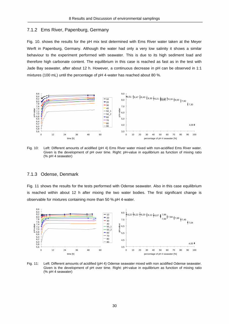
8 Results and Discussion of environmental samplings
30
7.1.2 Ems River, Papenburg, Germany
Fig. 10. shows the results for the pH mix test determined with Ems River water taken at the Meyer
Werft in Papenburg, Germany. Although the water had only a very low salinity it shows a similar
behaviour to the experiment performed with seawater. This is due to its high sediment load and
therefore high carbonate content. The equilibrium in this case is reached as fast as in the test with
Jade Bay seawater, after about 12 h. However, a continuous decrease in pH can be observed in 1:1
mixtures (100 mL) until the percentage of pH 4-water has reached about 80 %.
5,65,86,06,26,46,66,87,07,27,47,67,88,08,28,48,6
0 12 24 36 48 60
time [h]
pH
-val
ue
1020304050_150_260708090
8,51 8,47 8,43 8,30 8,21 8,058,18 8,16 8,00 7,82
7,30
4,00
3,0
4,0
5,0
6,0
7,0
8,0
9,0
0 10 20 30 40 50 60 70 80 90 100
percentage of pH 4 seawater [%]
pH
-val
ue
Fig. 10: Left: Different amounts of acidified (pH 4) Ems River water mixed with non-acidified Ems River water.Given is the development of pH over time. Right: pH-value in equilibrium as function of mixing ratio(% pH 4 seawater)
7.1.3 Odense, Denmark
Fig. 11 shows the results for the tests performed with Odense seawater. Also in this case equilibrium
is reached within about 12 h after mixing the two water bodies. The first significant change is
observable for mixtures containing more than 50 %.pH 4-water.
5,65,86,06,26,46,66,87,07,27,47,67,88,08,28,48,6
0 12 24 36 48 60
time [h]
pH
-val
ue
1020304050_150_260708090
8,22 8,22 8,20 8,12 8,077,84 7,69
7,457,04
7,99
7,93
4,00
3,5
4,5
5,5
6,5
7,5
8,5
0 10 20 30 40 50 60 70 80 90 100
percentage of pH 4 seawater [%]
pH-v
alu
e
Fig. 11: Left: Different amounts of acidified (pH 4) Odense seawater mixed with non acidified Odense seawater.Given is the development of pH over time. Right: pH-value in equilibrium as function of mixing ratio(% pH 4 seawater)
This document, and more, is available for download at Martin's Marine Engineering Page - www.dieselduck.net

8 Results and Discussion of environmental samplings
31
7.1.4 Calais, France
Fig. 12 shows the results obtained with Calais seawater. Noticeable in this case is that there is, for all
mixtures up to 60 % pH 4-seawater, no temporal behaviour of the pH until the equilibrium is reached.
For the rest of the mixtures equilibrium is reached after maximally 6 h. A change of the pH in
equilibrium out of the error range is first observable at a percentage of 60 % pH 4-seawater.
6,26,46,66,87,07,27,47,67,88,08,28,48,68,8
0 6 12 18 24 30 36
time [h]
pH-v
alu
e
1020304050_150_260708090
8,60 8,62 8,56 8,52 8,45 8,26 8,19 8,027,63
8,40
8,45
4,003,5
4,5
5,5
6,5
7,5
8,5
9,5
0 10 20 30 40 50 60 70 80 90 100
percentage of acidified (pH 4) seawater [%]pH
-va
lue
Fig. 12: Left: Different amounts of acidified (pH 4) Calais seawater mixed with non acidified Calais seawater.Given is the development of pH over time. Right: pH-value in equilibrium as function of mixing ratio(% pH 4 seawater)
7.1.5 Dover, England
A similar behaviour as observed for Calais seawater was found for Dover seawater. Fig. 13 shows the
results for this test. For a mixing ration of 50:50 no significant temporal development of the pH can be
observed. The first pH change in equilibrium greater than the error range is observable for
percentages greater than 50 % pH 4-seawater
6,06,26,46,66,87,07,2
7,47,67,88,08,28,4
0 12 24 36 48 60 72 84
time [h]
pH-v
alue
1020304050_150_260708090
8,27 8,21 8,14 8,10 8,05 7,90 7,77 7,577,09
7,99
7,95
4,003,5
4,5
5,5
6,5
7,5
8,5
9,5
0 10 20 30 40 50 60 70 80 90 100
percentage of pH4 seawater[%]
pH-v
alue
Fig. 13: Left: Different amounts of acidified (pH 4) Dover seawater mixed with non acidified Dover seawater.Given is the development of pH. Right: pH-value in equilibrium as function of mixing ratio (% pH 4seawater)
This document, and more, is available for download at Martin's Marine Engineering Page - www.dieselduck.net

8 Results and Discussion of environmental samplings
32
7.1.6 Comparison of all results (in equilibrium)
Looking at the figures Fig. 8 to Fig. 13 it can be seen that during the experiments with Ems river water,
Nassau harbour and Odense seawater the mixtures are in equilibrium after about the same time. For
Dover and Calais seawater, equilibrium is reached much faster.
In equilibrium all values, even the river water values, are about the same. Highest values were
observed for Calais seawater. Dover Jade and Odense values in equilibrium are, when error range of
the pH meter is taken in consideration, the same for all mixtures.
3,84,24,65,05,45,86,26,67,07,47,88,28,69,0
0 10 20 30 40 50 60 70 80 90 100
percentage of pH 4 seawater[%]
pH
-val
ue
JadeOdenseEmsCalaisDover
8,33 8,33 8,29 8,22 8,17 8,10 8,00 7,877,67
7,21
4,003,84,24,65,05,45,86,26,67,07,47,88,28,69,0
0 10 20 30 40 50 60 70 80 90 100
percentage of pH 4 seawater[%]
pH-v
alu
e
Fig. 14: Left: pH-value in equilibrium of mixing ratio (% pH 4 seawater) for all pH tests. Right: Mean of all testswith standard deviation.
3,8
4,2
4,6
5,0
5,4
5,8
6,2
6,6
7,0
7,4
7,8
8,2
8,6
9,0
0 10 20 30 40 50 60 70 80 90 100
percentage of pH 4 seawater[%]
pH-v
alu
e
d pH/ d percentage
0,00
0,05
0,10
0,15
0,20
0,25
0,30
0,35
0 10 20 30 40 50 60 70 80 90 100percentage of pH 4 seawater in mixture
Fig. 15: Left: mean pH value (points) and standard deviation (error bars) in equilibrium of mixing ratio (% pH 4seawater) for all pH tests. The black line shows the model fitted to the points and the red line showsthe 95 % confidence interval of the model. Right: change of pH over percentage
From all pH values determined for the different mixtures in equilibrium the mean and the standard
deviation was calculated and plotted against the percentage of the pH 4 water in the mixture. For
these values an easy function was searched which fits the values best. Therefore the free available
software LAB fit (LAB fit Curve fitting software V 7.2.6.) was used. The determined function
percentagedpercentagecb
percentageavaluepH
(12)
This document, and more, is available for download at Martin's Marine Engineering Page - www.dieselduck.net

8 Results and Discussion of environmental samplings
33
was then fitted to the data by using the software Systat 8.0 (command file see appendix). The result is
shown in Fig. 15. The raw R-square (1-Residual/Total), the mean corrected R-square (1-
Residual/Corrected) and the R (observed vs. predicted) square values, which were calculated with
Systat, equalled 1.000.
The values obtained are listed in Table 15. For 0 % the pH is defined asbapH .
Table 15: Values obtained by fitting equation 12 to the pH-values
parameter low 95 % optimum up 95 %A -101.784 -101.646 -101.508B -12.209 -12.1645 -12.120C 0.117 0.117793 0.118D -0.004 -0.00273782 -0.002
According to this function it is possible to mix natural seawater with acidified seawater in a relation of
60:40 to give a pH change of 0.2 pH units. According to the EPA regulations 0.2 units is maximum
allowed pH change in the initial mixing zone.
This document, and more, is available for download at Martin's Marine Engineering Page - www.dieselduck.net

8 Results and Discussion of environmental samplings
34
7.2 GC-MS Validation
For GC MS validation, one time three different dilution series with concentrations of 1, 10, 50 and
100 ng l-1 and one series made of 9 dilutions (2.5, 25, 25, 50, 50, 100, 250, 500, 1000 µg l-1) in which
some dilutions were prepared double but were diluted down from different concentrations. From this
series one of the 25 µg l-1 and the 500 µg l-1 concentrations were measured 8 times.
The three different dilution series were prepared to estimate the error due to the handling and the
diluting (Table 16). The calibration series with the nine different steps was prepared to determine the
linearity of the GC MS and the 8-fold measurements were performed to determine the accuracy of the
GC MS including the integration of the peak areas.
From Table 10 it can be seen that the relative standard error for the three different dilution series is
low. As the stock solution is a mix of all PAHs, it is admissible to calculate the mean of all compounds.
Therefore the error concerning to handling, loss to the walls of the vessels and additionally the GC MS
is 5.4 %. The accuracy of the GC MS alone is listed in Table 17.
The accuracy for the low molecular weight PAHs is higher than for the high molecular PAHs. The
difference between the relative standard deviations of low and high concentrations is to due to to
mathematical reasons. If the peak area error is always the same, the relative error is higher for low
peak areas than for higher peak areas. As all samples were concentrated within the range of 25 to
500 ng mL-1 it is admissible to calculate the mean of all standard deviations, which results in 2.5 %.
This is about the half of the relative standard deviation calculated for the three different dilution series.
Table 16: Standard deviation of three different standard dilution series.
compound rel. stand dev.acenaphthylene 4.7acenaphthene 4.7acenaphthene-D10 9.7fluorene 4.9phenanthrene-D10 4.5anthracene 6.0phenanthrene 5.1fluoranthene 4.1pyrene 5.8benz[a]anthracene 6.4chrysene-D12 6.8chrysene 9.7benzo[b]+benzo[k]fluoranthene 5.4benzo[a]pyrene 4.1perylene-D12 3.6dibenz[a,h]anthracene 2.4benzo[ghi]perylene 3.7indeno(1,2,3,c,d)pyrene 5.1mean 5.4
This document, and more, is available for download at Martin's Marine Engineering Page - www.dieselduck.net

8 Results and Discussion of environmental samplings
35
Table 17: Accuracy of the GC/MS analysis (including InjSTD, integration and measurement)
compound mean25 µg L-1
std. dev.25 µg L-1
rel. std. dev.25 µg L-1
mean500 µg L-1
std. dev.500µg l-1
rel. std. dev.500 µg L-1
acenaphthylene 0.133 0.002 1.4 2.865 0.015 0.5acenaphthene 0.086 0.001 1.4 1.848 0.009 0.5acenaphthene-D10 0.066 0.001 0.8 1.407 0.006 0.4fluorene 0.092 0.002 1.6 2.029 0.011 0.5phenanthrene-D10 0.110 0.001 0.8 2.382 0.007 0.3phenanthrene 0.142 0.002 1.2 3.117 0.019 0.6anthracene 0.133 0.002 1.1 2.982 0.019 0.7fluoranthene 0.134 0.002 1.2 2.978 0.016 0.5pyrene 0.135 0.002 1.8 2.975 0.017 0.6benz[a]anthracene 0.090 0.005 5.5 2.449 0.069 2.8chrysene-D12 0.083 0.003 3.1 2.281 0.018 0.8chrysene 0.103 0.004 3.8 2.707 0.032 1.2benzo[b]fluoranthene+benzo[k]fluoranthene
0.168 0.009 5.4 4.608 0.072 1.6
benzo[a]pyrene 0.056 0.004 7.2 1.609 0.045 2.8perylene-D12 0.045 0.003 6.5 1.263 0.031 2.4dibenz[a,h]anthracene 0.028 0.003 9.4 0.868 0.033 3.8benzo[ghi]perylene 0.040 0.002 5.9 1.065 0.024 2.3indeno(1.2.3.c.d)pyrene 0.030 0.002 7.5 1.015 0.031 3.0
Table 18: F-Test for linearity of the GC/MS analysis. Shown results were calculated for all dilution steps rangingfrom 2.5 to 1000 µg L-1
compound 2_linearys 2
_ nonlinearys DS² EV F (1.6)
acenaphthylene 33.39 13.75 151.27 11.00 13.745 linearacenaphthene 33.39 13.75 151.27 11.00 13.745 linearacenaphthene-D10 20.01 6.03 103.93 17.24 13.745 linearfluorene 30.66 33.53 13.40 0.40 13.745 linearphenanthrene-D10 21.90 15.16 62.34 4.11 13.745 linearphenanthrene 33.10 35.98 15.79 0.44 13.745 linearanthracene 114.90 101.42 195.76 1.93 13.745 linearfluoranthene 111.32 85.86 264.07 3.08 13.745 linearpyrene 110.49 70.20 352.21 5.02 13.745 linearbenz[a]anthracene 1999.05 316.49 12094.41 38.21 13.745 nonlinearchrysene-D12 686.38 265.45 3211.96 12.10 13.745 linearchrysene 342.60 241.16 951.23 3.94 13.745 linearbenzo[b]fluoranthenebenzo[k]fluoranthene
2050.00 419.41 11833.50 28.21 13.745 nonlinear
benzo[a]pyrene 2410.91 222.39 15542.04 69.89 13.745 nonlinearperylene-D12 2583.90 277.91 16419.87 59.08 13.745 nonlineardibenz[a.h]anthracene 1834.48 125.87 12086.15 96.02 13.745 nonlinearbenzo[ghi]perylene 1558.59 190.58 9766.67 51.25 13.745 nonlinearindeno(1.2.3.c.d)pyrene 2554.00 343.29 15818.21 46.08 13.745 nonlinear
This document, and more, is available for download at Martin's Marine Engineering Page - www.dieselduck.net
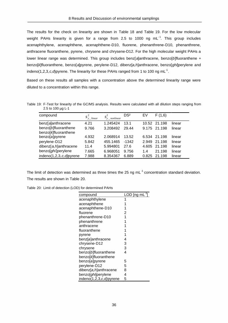
8 Results and Discussion of environmental samplings
36
The results for the check on linearity are shown in Table 18 and Table 19. For the low molecular
weight PAHs linearity is given for a range from 2.5 to 1000 ng mL-1. This group includes
acenaphthylene, acenaphthene, acenaphthene-D10, fluorene, phenanthrene-D10, phenanthrene,
anthracene fluoranthene, pyrene, chrysene and chrysene-D12. For the high molecular weight PAHs a
lower linear range was determined. This group includes benz[a]anthracene, benzo[b]fluoranthene +
benzo[k]fluoranthene, benzo[a]pyrene, perylene-D12, dibenz[a,h]anthracene, benzo[ghi]perylene and
indeno(1,2,3,c,d)pyrene. The linearity for these PAHs ranged from 1 to 100 ng mL-1.
Based on these results all samples with a concentration above the determined linearity range were
diluted to a concentration within this range.
Table 19: F-Test for linearity of the GC/MS analysis. Results were calculated with all dilution steps ranging from2.5 to 100 µg L-1
compound 2_ linearys 2
_ nonlinearys DS² EV F (1,6)
benz[a]anthracene 4.21 1.245424 13.1 10.52 21.198 linearbenzo[b]fluoranthenebenzo[k]fluoranthene
9.766 3.208492 29.44 9.175 21.198 linear
benzo[a]pyrene 4.932 2.068914 13.52 6.534 21.198 linearperylene-D12 5.842 455.1465 -1342 2.949 21.198 lineardibenz[a,h]anthracene 11.4 5.994801 27.6 4.605 21.198 linearbenzo[ghi]perylene 7.665 6.968051 9.756 1.4 21.198 linearindeno(1,2,3,c,d)pyrene 7.988 8.354367 6.889 0.825 21.198 linear
The limit of detection was determined as three times the 25 ng mL -1 concentration standard deviation.
The results are shown in Table 20.
Table 20: Limit of detection (LOD) for determined PAHs
compound LOD [ng mL-1]acenaphthylene 1acenaphthene 1acenaphthene-D10 1fluorene 2phenanthrene-D10 1phenanthrene 1anthracene 1fluoranthene 1pyrene 1benz[a]anthracene 4chrysene-D12 3chrysene 3benzo[b]fluoranthenebenzo[k]fluoranthene
4
benzo[a]pyrene 5perylene-D12 5dibenz[a,h]anthracene 8benzo[ghi]perylene 4indeno(1,2,3,c,d)pyrene 5
This document, and more, is available for download at Martin's Marine Engineering Page - www.dieselduck.net

8 Results and Discussion of environmental samplings
37
7.3 PAH-Extraction, Validation of Method
As in the most cases PAHs are extracted from fresh water or sediments most applications are fitted for
these matrices. Therefore tests (Chapter 4.2) were performed to determine the extraction efficiency,
the accuracy and the reproducibility of the method.
As there is no reference material for PAH in seawater available, for the recovery tests a certified PAH
mix in acetone was diluted, added to seawater and extracted as described before. The results of the
tests with the different SPE sorbents and the different elution solvents (Table 21) show that the best
recovery rate with the lowest standard deviation was obtained with the SPE C18ec cartridges and
DCM as elution solvent. The EASY material showed only low recovery rates (Fig. 16) for the high
molecular PAHs. The same was observed when using SPE C18ec and n-hexane (Fig. 17) as elution
solvent. Almost as good results as for C18ec and DCM were observed for C18 PAH SPE sorbent (Fig.
18). But as these cartridges were only available with a load of 500 mg, the flow was much slower and
the drying took longer than for C18ec. Therefore in all assays C18ec cartridges and DCM were used
to extract the soluble fraction of the PAHs. LLE also showed good recovery rates, but PAHs with high
vapour pressure were lost during evaporation in the rotary evaporator.
The recovery rate in natural seawater in Fig. 19 was low for high molecular PAHs when only the liquid
fraction was considered. Therefore additionally the filter was extracted. The results are shown in Fig.
21. Highest recovery rates close to 100 % were observed for fluorene, phenanthrene, pyrene and
dibenz[a,h]anthracene. The lowest recovery rate was determined for chysene-D12 with 66.4 %. The
mean recovery rate for all compounds was determined to be 86.1 % 10.6.
Fig. 20 shows that >90 % of acenaphthylene, acenaphthene, fluorene, phenanthrene-D10 and
anthracene are present in the dissolved form. Benzo[b]fluoranthene, benzo[k]fluoranthene,
benzo[a]pyrene, perylene-D12, dibenz[a,h]anthracene, benzo[ghi]perylene and indeno(1,2,3,c,d)
pyrene are mainly (>90 %) adsorbed to particles. Benz[a]anthracene, chrysene and chrysene-D12 are
distributed about 50:50 between particulate and aqueous phase. The results of this test showed that a
the highest recoveries were found after 2 h and 4 h. Extraction time had a significant influence on
phenanthrene, benz[a]anthracene, chrysene-D12 and chrysene only. For these compounds the
soluble fraction was rising with time.
This document, and more, is available for download at Martin's Marine Engineering Page - www.dieselduck.net

8 Results and Discussion of environmental samplings
38
0
20
40
60
80
100
120
acenaphth
ylene
acenaphth
ene-D10
fluor
en
phenan
thr en
e-D10
phenanthre
ne
anthracen
e
pyrene
benz[a
]anth
racene
chrysene-D
12
chrysene
benzo[b+k]
fluora
nth
benzo[ a]p
yrene
perylen-D
12
dibenz[
a,h]anth
racene
benzo[ghi]p
erylen
e
inden
o( 1,2,3,c
,d)p
yrene
0
20
40
60
80
100
120
acenaphth
ylene
acenapht hen
e-D10
fluore
n
phenanthre
ne-D10
phenanthre
ne
anthr acene
pyrene
benz[a]an th
race
ne
chr ysene-D
12
chrysen
e
benzo[ b+
k]fluora
nth
benzo[a
]pyre
ne
perylen-D
12
dibenz[a
,h]ant hr
acene
benzo[g
hi]pery
lene
indeno(1
,2,3,c
,d)p
yrene
Fig. 16: Results of tests for the determination of the recovery rates of PAHs from seawater. Left: Results ofLiquid-Liquid-Extraction. Shown are the recovery rates for the different PAHs and the overall mean andstandard deviation. Right: Same for extraction with SPE sorbent Chromabond EASY.
0
20
40
60
80
100
120
acenaphth
ylene
acenaphthene-D
10
fluor en
phenan
thr en
e-D10
phenanthre
ne
anthra
cene
pyrene
benz[a
]anth
racene
chrysen
e-D12
chrysene
benzo[b+k] flu
oranth
benzo[a] pyre
ne
peryle
n-D12
dibenz[a
,h]a
nthra
cene
benzo[g
hi]pery
lene
indeno(1
,2,3,c
,d)p
yrene
0
20
40
60
80
100
120
acenaphth
ylene
acenaphthene- D
10
fluor en
phenanth
rene-D
10
anthr ac
ene
phenanthre
ne
pyrene
benz[a
]anth
racene
chrysene-D
12
chrysene
benzo[b+k]f
luor anth
benzo[a
]pyre
ne
peryle
n-D12
dibenz[a
,h]a
nthra
cene
benzo[ghi] pery
lene
indeno(1
,2,3,c,d
)pyre
ne
Fig. 17: Results of tests for the determination of recovery rates of PAHs from seawater. Left: Extraction by SPEwith sorbent Chromabond C18 ec with elution solvent DCM. Shown are the recovery rates for thedifferent PAHs and the overall mean and standard deviation. Right: Same for SPE sorbentChromabond C18 ec but with elution solvent n-hexane.
0
20
40
60
80
100
120
acenaphth
ylene
acenaphth
ene-D10
fluor
en
phenan
thr en
e-D10
ant hr
acene
phenanth
r ene
pyrene
benz[a
]anthra
cene
chrysen
e-D12
chrysene
benzo[b+k]
fluora
nth
benzo[ a]
pyrene
peryle
n-D12
dibenz[a,h
]anthra
cene
benzo[ghi]p
erylene
inden
o( 1,2,3
,c,d)p
yrene
0
20
40
60
80
100
120
acenaphth
ylene
acenapht hen
e-D10
fluore
n
phenanthre
ne-D10
phenanthre
ne
anthr ac
ene
pyrene
benz[a]an
thra
cene
chr ysene-D
12
chrysen
e
benzo[ b+
k]fluora
nth
benzo[a
]pyre
ne
perylen-D
12
dibenz[a,h
]ant h
r acene
benzo[g
hi]pery
lene
indeno(1
,2,3,c,d
)pyre
ne
Fig. 18: Results of tests for the determination of recovery rates of PAHs from seawater. Left: Extraction by SPEwith sorbent Chromabond C18 PAH with elution solvent DCM. Shown are the recovery rates for thedifferent PAHs and the overall mean and standard deviation. Right: Influence of addition of differentamounts of acetone to the sample.
This document, and more, is available for download at Martin's Marine Engineering Page - www.dieselduck.net

8 Results and Discussion of environmental samplings
39
0
20
40
60
80
100
120
140
acenaphth
ylene
acenaphth
ene-D
10
fluore
n
p henanth
rene-D
10
phenanthr ene
anth
r acene
pyrene
b enz[a
]anth
racen
e
chrysene-D
12
chrysene
benzo[b+k]
fluor ant
h
benzo[ a]
pyrene
peryle
n-D12
diben
z[a,h
]anth
racene
benzo[ghi]p
erylene
inden
o( 1,2,3,c
,d)p
yrene
0
20
40
60
80
100
120
140
acenaphth
ylene
acenapht hen
e-D10
fluore
n
phenanth
rene-D
10
phenanthre
ne
ant hr
acene
pyrene
benz[a
]anth
racen
e
chrysene-D
12
chrysene
benzo[b+k]
fluor anth
benzo[a]p
yr ene
peryle
n-D12
dibenz[a
,h]a
nthra
cene
benzo[ghi]p
erylene
inden
o( 1,2,3,c
,d)p
yr ene
Fig. 19: Recovery rates of the soluble PAHs from natural seawater with Chromabond SPE sorbent C18 ec andelution solvent DCM. Left: Calais seawater Right: Dover seawater.
Table 21: Mean recovery rates and standard deviations determined for tests with artificial seawater.
PAH EASY C18PAH C18ec/ DCM C18ec/Hexane LLEmean sd mean sd mean sd mean sd mean sd
acenaphthylene 79.6 10.0 87.9 4.7 89.5 11.3 97.4 6.5 9.0 16.9acenaphthene-D10 76.3 9.8 76.3 6.4 80.8 8.5 90.1 8.0 8.3 18.3fluorene 87.8 12.0 89.6 9.6 94.4 16.2 105.5 11.0 13.2 24.4phenanthrene-D10 76.6 7.9 80.8 6.1 88.4 5.7 89.8 5.5 28.4 28.5phenanthrene 91.9 6.9 97.0 5.6 104.0 10.6 106.4 5.4 31.2 30.8anthracene 72.8 7.3 76.3 6.5 82.5 8.5 88.1 3.8 28.0 25.7pyrene 81.9 9.1 91.9 9.7 107.3 8.7 95.3 2.3 76.6 32.0benz[a]anthracene 59.0 2.8 67.9 5.1 92.2 8.1 57.9 4.1 75.5 6.3chrysene-D12 54.8 5.3 62.4 3.4 83.9 12.7 53.3 1.5 68.3 5.6chrysene 59.1 10.7 65.1 4.0 92.5 13.6 57.6 0.3 76.2 4.7benzo[b]fluoranthene+benzo[k]fluoranthene
45.6 3.3 66.7 4.4 78.1 5.7 49.9 2.7 74.1 3.5
benzo[a]pyrene 33.7 9.4 41.4 3.3 57.8 15.5 30.8 3.2 62.1 11.9perylene-D12 34.3 4.0 46.6 8.4 59.4 6.9 37.2 6.5 68.4 4.0dibenz[a,h]anthracene 33.5 7.4 61.1 3.2 69.3 9.5 41.3 0.1 72.6 16.5benzo[ghi]perylene 38.1 3.9 88.1 8.4 85.8 18.2 63.7 2.0 86.0 9.8indeno(1,2,3,c,d)pyrene 36.9 6.0 70.5 2.7 76.9 5.4 48.7 1.6 71.4 7.4mean + standard deviation 60.1 21.1 73.1 16.0 84.0 13.8 69.6 25.8 53.1 27.9
This document, and more, is available for download at Martin's Marine Engineering Page - www.dieselduck.net

8 Results and Discussion of environmental samplings
40
0
10
20
30
40
50
60
70
80
90
100
acen
aphth
ylene
acen
aphth
ene-
D10
f luoren
phen
anthr
ene-D10
anthr
acen
e
phen
anth
rene
pyren
e
benz
[a]an
thrac
ene
chrys
ene-D
12
chryse
ne
benz
o[b+k
] fluora
nth
benz
o[a]py
rene
peryl
en-D
12
diben
z[a,h
]anthr
acen
e
benz
o[ghi]
perylen
e
i nden
o(1,2
,3,c,d
)pyre
ne
1 h2 h4 h10 h
Fig. 20: Fractionation of PAHs between dissolved and particulate fraction after different incubation times.
79,8
88,2
99,9
90,4
101,6 86,1
96,6 70
,6
66,4
71,5
76,3
86,8
89,2
96,7
90,1
87,4
0
20
40
60
80
100
120
acen
apht
hylen
e
acen
apht
hene-D
10
fluor
en
phena
nthre
ne-D
10
anthr
acen
e
phen
anth
rene
pyren
e
benz[a
]ant
hrac
ene
chry
sene
-D12
chry
sene
benz
o[b+
k]flu
oran
th
benzo
[a]py
rene
peryle
n-D1
2
d ibenz
[a,h]
anth
race
ne
benz
o[gh
i]per
ylene
inden
o(1,2
,3,c,d
)pyr
ene
Fig. 21: Mean recovery rate and standard deviation for eight extractions of Dover seawater and particulatefraction.
This document, and more, is available for download at Martin's Marine Engineering Page - www.dieselduck.net
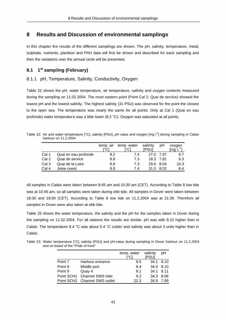
8 Results and Discussion of environmental samplings
41
8 Results and Discussion of environmental samplings
In this chapter the results of the different samplings are shown. The pH, salinity, temperature, metal,
sulphate, nutrients, plankton and PAH data will first be shown and described for each sampling and
then the variations over the annual circle will be presented.
8.1 1st sampling (February)
8.1.1 pH, Temperature, Salinity, Conductivity, Oxygen
Table 22 shows the pH, water temperature, air temperature, salinity and oxygen contents measured
during the sampling on 11.02.2004. The most eastern point (Point Cal 2: Quai de service) showed the
lowest pH and the lowest salinity. The highest salinity (31 PSU) was observed for the point the closest
to the open sea. The temperature was nearly the same for all points. Only at Cal 1 (Quai en eau
profonde) water temperature was a little lower (8.2 °C). Oxygen was saturated at all points.
Table 22: Air and water temperature [°C], salinity [PSU], pH value and oxygen [mg l-1] during sampling in Calaisharbour on 11.2.2004
temp. air[°C]
temp. water[°C]
salinity[PSU]
pH oxygen[mg L-1]
Cal 1 Quai en eau profonde 8.2 7.4 27.0 7.97 9.7Cal 2 Quai de service 8.8 7.3 18.3 7.81 9.3Cal 3 Quai de la Loire 8.8 7.3 29.6 8.04 10.3Cal 4 Jetee ouest 8.8 7.4 31.0 8.02 8.4
All samples in Calais were taken between 8:45 am and 10:30 am (CET). According to Table 8 low tide
was at 10:45 am, so all samples were taken during ebb tide. All samples in Dover were taken between
18:30 and 19:00 (CET). According to Table 8 low tide on 11.2.2004 was at 21:39. Therefore all
samples in Dover were also taken at ebb tide.
Table 23 shows the water temperature, the salinity and the pH for the samples taken in Dover during
the sampling on 11.02.2004. For all stations the results are similar. pH was with 8.10 higher than in
Calais. The temperature 8.4 °C was about 0.4 °C colder and salinity was about 3 units higher than in
Calais.
Table 23: Water temperature [°C], salinity [PSU] and pH-value during sampling in Dover harbour on 11.2.2004and on board of the “Pride of Kent”
temp. water[°C]
salinity[PSU]
pH
Point 7 Harbour entrance 8.5 34.1 8.10Point 8 Middle port 8.4 34.0 8.10Point 9 Quay 4 8.1 34.1 8.11Point SCH1 Channel SWS inlet 9.2 34.3 8.06Point SCH2 Channel SWS outlet 22.3 34.9 7.99
This document, and more, is available for download at Martin's Marine Engineering Page - www.dieselduck.net

8 Results and Discussion of environmental samplings
42
Despite dilution by the cooling water the temperature was higher in the outflow than in the inlet water
(inlet 9.2 °C outlet 22.3°C). Although this increase will have no or only little direct influence on the
ecosystem it will influence the physical behaviour of the effluent. Higher temperatures at constant
salinity increase the buoyancy of the effluent in comparison to the surrounding water. This may
partially hinder the water bodies from effective mixing. A change in salinity, which would support or
reduce this effect, was not observed. Another effect of higher water temperatures is the lower solubility
of gaseous compounds in warmer water. This could lead to oxygen depletion. As oxygen was
saturated in all samples no adverse effect was observed. Besides, a negative effect of cooling water
discharges from ships on the surrounding environment was, concerning to the knowledge of the
author, never reported.
8.1.2 Metals and Sulphate
Metal and sulphate concentrations determined by ICP-OES are shown in Table 25. The determined
metals are listed in chapter 5.3 on page 15. Concentrations below the detection limit are marked by a
dash. The concentration of the sea salt standard (International Association for Physical Science of the
Ocean, IAPSO) are given in Table 24.
Table 24: Contents of the International Association for Physical Science of the Ocean standard for naturalAtlantic seawater.
element Ba Ca Cd Co Cr Cu Fe K Li Mgunit ppb ppm ppb ppb ppb ppb ppb ppm ppb ppmconcentration 14 412 0.01 0.05 0.04 0.1 2 387 180 1294
element Mn Mo Ni Pb SO4 Sr V Znunit ppb ppb ppb ppb ppm ppb ppb ppbconcentration 0.2 10 0.2 0.003 2712 8000 2.5 0.1
During the sampling on 11.2.2003 none of the examined transition metals were found inside the
harbours with the exception of Calais point Cal 2: Quai de service. Here a manganese concentration
of 69 ppb was detected. At this point earth metals were with the exception of barium lower in
comparison to the other points, whereas at the harbour entrance in Dover Ba, Li, Sr, Ca, K and Mg
concentrations were slightly higher than at the other points. The sulphate concentration was highest at
this point too. Both, the high sulphate and the high earth metal concentrations are mainly due to the
higher salinity at this point. The comparison between seawater scrubber inlet and outlet water showed
a slight increase of the zinc concentration in the outlet water. This is most probably due to a
contamination from for example the tubing, the fittings or the pumps.
This document, and more, is available for download at Martin's Marine Engineering Page - www.dieselduck.net

8 Results and Discussion of environmental samplings
43
Table 25: Sulphate, earth and transition metals determined for the samples taken on 11.02.2004. Fields with”-“show concentrations below the detection limit.
Cal 1 Cal 2 Cal 3 Cal 4 7 8 9 21 22Ba ppb 17 21 18 16 20 14 14 13 12Ca ppm 339 263 359 369 509 391 390 395 401Cd ppb - - - - - - - - -Co ppb - - - - - - - - -Cr ppb - - - - - - - -Cu ppb - - - - - - - - -Fe ppb - - - - - - - - -K ppm 280 180 310 352 475 352 373 357 376Li ppb 148 112 161 169 232 185 186 181 185Mg ppm 994 664 1071 1113 1567 1183 1191 1219 1254Mn ppb - 68 - - - - - - -Mo ppb - - - - - - - - -Ni ppb - - - - - - - - -Pb ppb - - - - - - - - -SO4 ppm 2161 1479 2399 2461 3831 2857 2853 2842 2874Sr ppb 6392 4448 6853 7223 10188 7889 7863 7907 8093V ppb - - - - - - - - -Zn ppb - - - - - - - - 143
8.1.3 Nutrients
Table 26 shows the nutrients concentrations determined for the samples taken on 11.02.2004. The
following abbreviations are used. Total chlorophyll (THCL), particulate inorganic phosphorus (PIP),
particulate organic phosphorus (POP), total particulate phosphorus (TPP), reactive dissolved
phosphorus (RDP), dissolved organic phosphorus (DOP), total dissolved phosphorus (TDP), dissolved
inorganic nitrogen (DIN).
The chlorophyll concentration was highest at point Cal 4 and lowest in the seawater scrubber outlet. At
point Cal 4 also the phosphorus and nitrogen compounds were high, but highest at point Cal 2. This
might indicate a higher amount of diatoms or a starting bloom.
Table 26: Nutrient concentrations determined for the samples taken on 11.02.2004
TCHL Seston PIP POP TPP RDP DOP TDP[µg L-1] [mg L-1] [µmol L -1] [µmol L-1] [µmol Ll-1] [µmol L-1] [µmol L-1] [µmol L-1]
Cal 1 2.2 62.8 0.80 0.70 1.50 0.51 8.14 8.65Cal 2 2.6 39.1 0.88 0.82 1.69 5.23 5.28 10.51Cal 3 2.7 42.5 0.25 0.38 0.63 0.70 5.42 6.12Cal 4 6.6 138.6 0.08 0.82 0.90 0.51 6.12 6.637 (Dover) 2.5 122.7 0.25 0.58 0.83 0.26 5.43 5.698 (Dover) 2.4 120.8 0.22 0.60 0.82 0.35 3.52 3.889 (Dover) 3.0 108.8 0.29 0.42 0.71 0.35 2.83 3.18
SCH1 1.4 75.1 0.10 0.36 0.45 0.35 4.20 4.55SCH2 0.9 55.3 0.05 0.32 0.36 0.26 4.97 5.23
This document, and more, is available for download at Martin's Marine Engineering Page - www.dieselduck.net

8 Results and Discussion of environmental samplings
44
NO2- NO3
- NH4+ DIN Si(OH)4
[µmol L-1] [µmol L-1] [µmol L-1] [µmol L-1] [µmol L-1]Cal 1 0.90 42.09 24.31 67.30 54.27Cal 2 2.03 74.66 107.64 184.32 92.78Cal 3 1.15 61.89 15.29 78.33 34.95Cal 4 0.74 41.86 10.41 53.02 24.507 (Dover) 0.22 15.97 1.49 17.69 6.318 (Dover) 0.23 15.21 18.96 34.40 6.579 (Dover) 0.44 20.10 19.25 39.79 9.38SCH1 0.33 16.41 1.53 18.26 5.63SCH2 0.22 11.41 1.53 13.16 7.37
8.1.4 Polycyclic Aromatic Hydrocarbons
Table 69 gives the total amounts of the 16 EPA-PAHs (without naphthalene), n Table 70 the
concentrations of the dissolved and the particulate are shown. The highest concentration was
determined for point Cal 4: Jetee Ouest, the lowest concentration for point Cal 3 Quai de la Loire. For
points Cal 2 and Cal 3 total concentrations of 267 ng L-1 and 354 ng L-1 were determined. In all cases
phenanthrene was dominating and only at point 4 a higher amount of low molecular weight PAHs was
found.
In Dover at all sampling points the PAH amounts were about equally high, and in the same order of
magnitude as in Calais. The dominating compound was in Dover phenanthrene too. High molecular
weight PAHs had extremely low contents.
The PAH contents determined for the Ecosilencer inlet and outlet are shown in Table 72. In these
samples phenanthrene was dominating too. The total amount of PAHs determined at the outlet was
16-fold higher than the amount determined in the inlet water. In the outlet water the particulate fraction
was about five times higher than the dissolved fraction.
To determine whether the PAHs are similarly distributed and show similar patterns a regression of the
compounds was performed. The results are shown in Table 28. It can be seen that the range of the
correlation coefficients is widely distributed from not significant to 0.999. Highest R² values were
observed between the more soluble two- and three-ring compounds whereas the relation between the
soluble and insoluble PAHs is lower. As this method might be influenced by great differences in
concentrations of the single compounds a regression of the concentrations at the different sampling
points was performed (Table 27). The difference between these two approaches is that the regression
of the compounds shows high correlation coefficients if for example anthracene is high at all points
where phenanthrene is low. The correlation coefficient for the regression of the sampling points
reflects the relation of all compounds to each other. The regression of the sampling points delivered
high correlations coefficients for all regressions. This indicates that the PAHs are similarly distributed
at all points. The results of the compound regression are shown in Table 28. It can be seen that the
low molecular weight PAHs are highly correlated with the remaining low molecular weight PAHs and
the high molecular weight PAHs with the remaining high molecular weight PAHs. But the high
molecular compounds are not correlated with the low molecular compounds. This shows that the PAH
This document, and more, is available for download at Martin's Marine Engineering Page - www.dieselduck.net

8 Results and Discussion of environmental samplings
45
load of the water has a similar composition at all points, whereas the PAHs bound to particles show a
different composition.
Table 27: Regression of sample points (Sampling 11.2.04). Colours are added for a better visualisation. Yellow -highly correlated, red - moderate or low correlation, dark red - no significant. correlation.
Cal
1
Cal
2
Cal
3
Cal
4
7 8 9 SC
H1
SC
H2
Cal1 1 0.997 0.987 0.874 0.995 0.95 0.997 0.999 0.982
Cal2 1 0.986 0.855 0.995 0.951 0.992 0.995 0.986
Cal3 1 0.859 0.99 0.937 0.979 0.989 0.978
Cal4 1 0.833 0.822 0.884 0.865 0.786
7 1 0.946 0.987 0.997 0.993
8 1 0.947 0.947 0.932
9 1 0.995 0.97
SCH1 1 0.985
SCH2 1
Table 28: Regression of compound contents determined for the samples taken on 11.2.04. Colours are added fora better visualisation. Yellow - highly correlated, red - moderate or low correlation, dark red - nosignificant correlation.
AT
HY
AT
HE
FLR
E
PH
EN
AN
TH
FLU
A
PY
R
BaA
CH
RY
Bbk
F
BaP
Dah
A
Bgh
iP
IND
EATHY 1 0.994 0.988 0.988 0.954 0.989 0.746 NS 0.405 NS NS NS NS NSATHE 1 0.995 0.995 0.967 0.995 0.753 NS 0.412 NS NS NS NS NSFLRE 1 0.999 0.965 0.997 0.738 NS 0.404 NS NS NS NS NSPHEN 1 0.969 0.999 0.756 NS 0.418 NS NS NS NS NSANTH 1 0.971 0.778 NS 0.419 NS NS NS NS NSFLUA 1 0.779 NS 0.441 NS NS NS NS NSPYR 1 0.497 0.821 0.418 0.403 NS 0.309 0.304BaA 1 0.665 0.672 0.571 NS 0.435 0.417CHRY 1 0.71 0.742 NS 0.602 0.567BbkF 1 0.959 NS 0.913 0.835BaP 1 NS 0.915 0.814DahA 1 NS NSBghiP 1 0.957INDE 1
This document, and more, is available for download at Martin's Marine Engineering Page - www.dieselduck.net
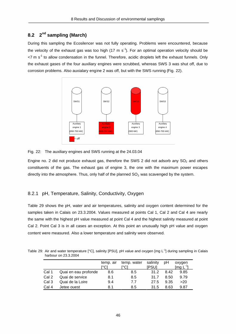
8 Results and Discussion of environmental samplings
46
8.2 2nd sampling (March)
During this sampling the Ecosilencer was not fully operating. Problems were encountered, because
the velocity of the exhaust gas was too high (17 m s-1). For an optimal operation velocity should be
<7 m s-1 to allow condensation in the funnel. Therefore, acidic droplets left the exhaust funnels. Only
the exhaust gases of the four auxiliary engines were scrubbed, whereas SWS 3 was shut off, due to
corrosion problems. Also auxialary engine 2 was off, but with the SWS running (Fig. 22).
SWS1 SWS2 SWS3 SWS3
Auxiliary
engine 1
(650-700 kW)
Auxiliary
engine 2
(650-700 kW)
Auxiliary
engine 3
(900 kW)
Auxiliary
engine 4
(650-700 kW)
= off
Fig. 22: The auxiliary engines and SWS running at the 24.03.04
Engine no. 2 did not produce exhaust gas, therefore the SWS 2 did not adsorb any SO2 and others
constituents of the gas. The exhaust gas of engine 3, the one with the maximum power escapes
directly into the atmosphere. Thus, only half of the planned SO2 was scavenged by the system.
8.2.1 pH, Temperature, Salinity, Conductivity, Oxygen
Table 29 shows the pH, water and air temperatures, salinity and oxygen content determined for the
samples taken in Calais on 23.3.2004. Values measured at points Cal 1, Cal 2 and Cal 4 are nearly
the same with the highest pH value measured at point Cal 4 and the highest salinity measured at point
Cal 2. Point Cal 3 is in all cases an exception. At this point an unusually high pH value and oxygen
content were measured. Also a lower temperature and salinity were observed.
Table 29: Air and water temperature [°C], salinity [PSU], pH value and oxygen [mg L-1] during sampling in Calaisharbour on 23.3.2004
temp. air[°C]
temp. water[°C]
salinity[PSU]
pH oxygen[mg L-1]
Cal 1 Quai en eau profonde 8.6 8.5 31.2 8.42 9.85Cal 2 Quai de service 8.1 8.5 31.7 8.50 9.79Cal 3 Quai de la Loire 9.4 7.7 27.5 9.35 >20Cal 4 Jetee ouest 8.1 8.5 31.5 8.63 9.87
This document, and more, is available for download at Martin's Marine Engineering Page - www.dieselduck.net

8 Results and Discussion of environmental samplings
47
All samples in Calais were taken between 16:00 and 18:30 (CET). According to Table 8 high tide was
at 14:21 and therefore samples were taken at ebb tide.
Table 30 shows the pH, water and air temperatures, salinities and oxygen contents determined for the
samples taken in Dover on 24.03.2004. The samples from points 5 and 6 were taken between 8:40
and 10:00 (Table 9) and therefore shortly after low tide (Table 8). Samples at point 7, 8 and 9 were
taken between 13:15 and 13:35 and therefore quite exactly at high tide. The lowest temperature was
measured at point 6 the other values determined for this point are about the same as those measured
close to the „Pride of kent“. The sample take at the beach at point 5 had the lowest salinity and the
lowest pH.
Table 30: Air and water temperatures [°C], salinity [PSU], pH value and oxygen [mg L-1] during sampling in Doverharbour on 24.3.2004
Dover temp. air[°C]
temp. water[°C]
salinity[PSU]
pH oxygen[mg L-1]
Point 5 Churchill Hotel Beach 9.0 11.0 27.0 7.68 9.52Point 6 Prince of Wales pier 7.4 8.9 34.3 7.86 10.1Point 7 Back of „Pride of kent“ 12.3 8.8 34.2 7.95Point 8 Middle of „Pride of kent“ 12.3 8.8 34.4 7.95Point 9 Front of „Pride of kent“ 12.3 8.8 34.4 8.00
Table 31 shows the pH, the salinities and the temperatures measured inside the seawater scrubber
system. Looking at the inlet samples, the temperature was highest inside the Channel (15.2°C). The
lowest salinity was measured in Calais (32.9) and the lowest pH (7.72) in Dover. If these values are
compared with the values at the outlet it can be seen that the salinity was slightly increased and the
temperature was raised by about 2 °C to 3 °C. The pH was lowered in all cases. The strongest
reduction was observed in the channel where the difference between inlet and outlet pH was 1.16 pH
units whereas in Calais and in Dover it was 0.66 and 0.43, respectively.
Table 31: Water temperature [°C], salinity [PSU], pH value and oxygen [mg L-1] during sampling on the “Pride ofKent” on 24.3.2004
temp. water[°C]
salinity[PSU]
pH
SD1 seawater inlet Dover 10.7 34.2 7.72SD2 seawater outlet Dover 14.8 34.6 7.29SCH1 seawater inlet Channel 15.2 34.9 7.94SCH2 seawater outlet Channel 17.1 35.2 6.78SCH3 outlet from US filter 27.6 35.5 2.73SCH4 to settling tank 28.8 35.4 2.86SCH5 inlet to US filter 27.9 35.2 2.82SCH6 return from Ecosilencer 28.0 35.2 2.78SCH7 top of settling tank 27.2 33.5 2.83SCH8 bottom of settling tank 23.0 34.9 2.83SC1 seawater inlet Calais 9.5 32.9 8.00SC2 seawater outlet Calais 12.8 32.9 7.34
This document, and more, is available for download at Martin's Marine Engineering Page - www.dieselduck.net

8 Results and Discussion of environmental samplings
48
The values determined for the samples taken from the remaining seawater scrubber points show, with
the exception of the settling tank, no change in salinity. Inside the settling tank the salinity was lower
perhaps because the water remains there for a while and therefore water from different water bodies
is mixed. The remaining time of the water inside the settling tank might also be an explanation why
there the pH is higher than pH 3 as in comparison to the remaining seawater scrubber points, where it
is lower than 3. Although the effluent water had a significantly lower pH than the inflowing water, no
pH change in the harbour or close to the “Pride of Kent” was measured. Additionally there was no pH
change observable inside the harbour between the first sampling where the Ecosilencer was not
running and the second sampling.
8.2.2 Metals and Sulphate
Sulphate, transition and earth metal concentrations of the harbour and the Ecosilencer samples taken
on 23/24.03.2004 are given in Table 32. Inside the ports a copper concentration of 220 ppb in Calais
at point Cal 1 and a zinc concentration of 53 ppb at point 9 in Dover were observed. Sulphate
concentrations were highest in Dover at the Prince of Wales Pier and at Terminal 4 (back of “Pride of
Kent”, Point 9). The samples taken in the middle (point 8) and at the front (point 7) of the „Pride of
Kent“ show lower earth metal and sulphate conentents than the other samples.
Inside the seawater scrubber system the highest transition metal contents were determined for the
samples taken from the tube to the settling tank and inside the settling tank. Additionally, high copper
and zinc concentrations were found at the inlet to the US filter. Except for iron (789 ppb) no metals
could be detected directly after the Ecosilencer. This indicates that most metals are leached from the
tubing due to the low pH and do not originate from the fluegas scrubbing process itself. At the outlet of
the US filter only vanadium (183 ppb) was determined and in the SWS outlet sample taken in the
Channel and in Dover, zinc (138 ppb and 537 ppb) was detected. Inside the seawater scrubber
system highest transient metal concentrations were found at the inlet to and inside the settling tank.
This indicates that most of the metals are bound to particles or are particulates themselves and are
therefore effectively removed from the system.
Sulphate concentrations did show an increase inside the SWS directly after the Ecosilencer but this
increase was diluted to the SWS inlet sulphate level before it left the „Pride of Kent“. Inside the
harbours the sulphate concentrations are at about the same level as the effluent concentrations but
due to different salinity values they vary within a range of 1500 and 3350 ppm.
This document, and more, is available for download at Martin's Marine Engineering Page - www.dieselduck.net

8 Results and Discussion of environmental samplings
49
Table 32: Sulphate, earth and transition metal contents determined for the samples taken in July
Cal 1 Cal 2 Cal 3 Cal 4 5 6 7 8 9 SD1 SD2 SCH2 SCH1 SCH3 SCH4 SCH5 SCH6 SCH7 SCH8 SC1 SC2Ba ppb 18 20 22 18 23 19 18 15 19 16 17 16 21 18 34 19 19 24 26 18 19Ca ppm 382 356 348 380 341 398 327 279 371 395 397 405 406 411 434 404 396 396 562 381 370Cd ppb - - - - - - - - - - - - - - - - - - - - -Co ppb - - - - - - - 8 - - - - - - - - - - - - -Cr ppb - - - - - - - - - - - - - - 264 - - - - - -Cu ppb 220 - - - - - - - - 129 129 - - - 7089 10978 - 273 2127 - -Fe ppb - - - - - - - - - - - - - 1051 5283 892 789 1508 - - -K ppm 352 345 314 366 288 398 340 297 381 397 384 428 426 434 437 422 419 405 424 388 367Li ppb 164 158 147 165 140 178 150 128 169 188 188 187 185 185 185 183 180 175 183 172 166Mg ppm 1154 1091 1007 1161 980 1251 1028 883 1173 1213 1202 1278 1278 1290 1289 1272 1245 1207 1255 1189 1149Mn ppb - - - - - - - - - - 20 - - - 72 - - - 332 - -Mo ppb - - - - - - - - - - - - - - - - - - 403 - -Ni ppb - - - - - - - - - - - - - - 277 - - - 1076 - -Pb ppb - - - - - - - - - - - - - - - - - - - - -SO4 ppm 2619 2625 2307 2628 2277 2920 2342 1942 2955 2949 2962 2990 3052 3342 3380 3359 3550 3235 3419 2920 2938Sr ppb 7220 6829 6345 7202 6160 7730 6410 5490 7308 7987 8024 8031 7953 8074 8193 7950 7830 7616 8491 7487 7151V ppb - - - - - - - - - - - - - 183 320 - - - - - -Zn ppb - - - - - - - - 53 - 537 - 138 - 1033 1461 655 414 98 - -
For a better visualisation and a better estimate of the SWS influence a comparison between the
sulphate, transition and earth metal concentration determined for the SWS inlet and outlet is show in
Figs. 22 to 28 comparing the inlet and outlet samples taken in March and February. Samples taken on
11.02.2004 are marked, because during this sampling the seawater scrubber was not running. During
the sampling on 24.03.2004 copper was found in inlet and outlet samples taken in Dover. In both
samples the copper concentration was the same. In Dover also manganese was found, but only in the
outlet effluent. In all outlet but not in the inlet samples except in Calais on 24.03.2004 zinc was
determined. Earth metals were all, within the accuracy of the measurements, equally concentrated in
the inlet and outlet samples, only barium seems to be slightly increased, when the SWS is running.
Copper (Cu)Comparison between SWS Inlet and Outlet
129
129
0
20
40
60
80
100
120
140
Dover24.03. 04
Channel 24.03.04
Calais 24.03.04
Channel 11. 02.04
conc
entra
tion
[ppb
]
InletOutlet
+below
= detectionlimit
IAPSO= 0 ppb
+ + + + + +
Manganese (Mn)Comparison between SWS Inlet and Outlet
20
0
5
10
15
20
25
Dover 24.03.04
Channel 24.03.04
Calai s24.03.04
Channel 11.02.04
conc
entra
tion
[ppb
]
InletOutlet
+below
= detectionlimit
IAPSO= 0
+ + + + + ++
Fig. 23: Left: Copper content [ppb]. Right: Manganese content [ppb] determined for Ecosilencer inlet and outletsamples taken in Calais, Dover and the Channel on 23/24.03.2004 and on 11.02.2004. IAPSO: Atlanticwater salinity standard.
This document, and more, is available for download at Martin's Marine Engineering Page - www.dieselduck.net

8 Results and Discussion of environmental samplings
50
Zinc (Zn)Comparison between SWS Inlet and Outlet
537
138
143
0
100
200
300
400
500
600
Dover 24.03 .04
Cha nne l 24.0 3.04
Calais24.03 .04
Chan nel 11 .02.0 4
con
cent
ratio
n[p
pb]
InletOutlet
+below
= detectionlimit
IAPSO= 0 ppb
++ + + +
Barium (Ba)Comparison between SWS Inlet and Outlet
16
16
1817
21 19
13 12
0
5
10
15
20
25
30
35
Do ver 2 4.03 .04
Cha nnel 24.03 .04
Calais24.03 .04
Chan nel 1 1.02 .04
con
cent
ratio
n[p
pb]
InletOutlet
- = IAPSO
Fig. 24: Left: Zinc content [ppb]. Right: Barium content [ppb] determined for Ecosilencer inlet and outletsamples taken in Calais, Dover and the Channel on 23/24.03.2004 and on 11.02.2004. IAPSO: Atlanticwater salinity standard.
Lithium (Li)Comparison between SWS Inlet and Outlet
188
187 172
181
188
185 166
185
0
50
100
150
200
250
Dover 24.03 .04
Cha nne l 24.0 3.04
Calais 24.03 .04
Chan nel 11 .02.0 4
con
cen
tra
tion
[pp
b]
InletOutlet
- = IAPSO
Strontium (Sr)Comparison between SWS Inlet and Outlet
7987
8031
7487
7907
8024
7953
7151
8093
0
1000
2000
3000
4000
5000
6000
7000
8000
9000
Do ver 2 4.03 .04
Cha nnel 2 4.03 .04
Calais 24 .03.0 4
Ch anne l 11.0 2.04
con
cen
tra
tion
[pp
b]
InletOutlet
- = IAPSO
Fig. 25: Left: Lithium content [ppb]. Right: Strontium content [ppb] determined for Ecosilencer inlet and outletsamples taken in Calais, Dover and the Channel on 23/24.03.2004 and on 11.02.2004. IAPSO: Atlanticwater salinity standard.
Calcium (Ca)Comparison between SWS Inlet and Outlet
395
405
381
395
397
406 3
70
401
0
50
100
150
200
250
300
350
400
450
Dover 24.03 .04
Cha nne l 24.0 3.04
Calais 24.03 .04
Chan nel 11 .02.0 4
conc
entr
atio
n[p
pm
]
InletOutlet
- = IAPSO
Potassium (K)Comparison between SWS Inlet and Outlet
397
428 388 357
384
426 367
376
0
50
100
150
200
250
300
350
400
450
500
Dove r 24 .03.0 4
Chann el 24 .03.0 4
Calais 24 .03.0 4
Ch anne l 11.0 2.04
conc
entr
atio
n[p
pm
]
InletOutlet
- = IAPSO
Fig. 26: Left: Calcium content [ppm]. Right: Potassium content [ppm] determined for Ecosilencer inlet and outletsamples taken in Calais, Dover and the Channel on 23/24.03.2004 and on 11.02.2004. IAPSO: Atlanticwater salinity standard.
This document, and more, is available for download at Martin's Marine Engineering Page - www.dieselduck.net

8 Results and Discussion of environmental samplings
51
Magnesium (Mg)Comparison between SWS Inlet and Outlet
1213
1278
1189
1219
1202
1278
1149
1254
0
200
400
600
800
1000
1200
1400
Dover 24.0 3.04
Ch anne l 24.03 .04
Calais 2 4.03. 04
Ch anne l 11.0 2.04
con
cent
ratio
n[p
pm]
InletOutlet
- = IAPSO
Sulphate (SO4)Comparison between SWS Inlet and Outlet
2949
2990
2920
2842
2962
3052
2938
2874
0
500
1000
1500
2000
2500
3000
3500
Do ver 2 4.03 .04
Chan nel 2 4.03. 04
Ca lais 24 .03.0 4
Cha nnel 1 1.02 .04
con
cent
ratio
n[p
pm]
InletOutlet
- = IAPSO
Fig. 27: Left: Magnesium content [ppb]. Right: Sulphate content [ppb] determined for Ecosilencer inlet andoutlet samples taken in Calais, Dover and the Channel on 23/24.03.2004 and on 11.02.2004. IAPSO:Atlantic water salinity standard.
8.2.3 Nutrients
Table 26 shows the nutrient and seston contents determined for the samples taken in March. In Calais
the highest seston content was observed at point Cal 2 (50.9 mg L -1) where about double the content
of the remaining points was observed. Sampling point 5 was situated at a sandy beach therefore the
seston content was higher (80.9 mg l-1) in comparison to the sample taken at the Prince of Wales pier
where the seston content was comparable to those measured in Calais. On board of the „Pride of
Kent“ the highest contents where not observed inside the settling tank as expected, but in the outlet of
the US filter (132.0 mg L-1). Inside the pipe which leads the water to the settling tank also high particle
contents where observed. Looking at the inlet and the outlet samples it can be seen, that the highest
seston contents were observed in the inlet sample taken in Calais (262.6 mg L-1). This might be an
effect of the berthing, where the screws whirl up a lot of sediment, which then might be sucked into the
ships cooling cycle. In Calais and Dover the seston contents in the outlet are lower than those
observed in the inlet. That shows that the clean-up system inside the ship (cyclones, settling tank and
US filter) worked and removed these particles. It also explains the high content measured at point
SCH4 where the removed particles pass by.
Looking at the RDP, DOP and TDP values it can be seen that they are quite the same in Dover and
Calais. Only at point Cal 3 where the algal bloom was observed nearly doubled TDP concentrations
were determined. At this point also the DIN concentrations were very high and only inside the settling
tank higher concentrations were measured. In both samples these high concentrations are due to by
high ammonia values; 33.05 µmol L-1 at point Cal 3 and 76.66 µmol L-1 at point SCH8 were observed,
whereas at the remaining points the concentrations varied between 1.34 and 12.81 µmol L-1. A nitrate
increase in the outlet samples in comparison to the inlet samples was only observed in Dover and
inside the Channel. In Calais the inlet sample contained more nitrate (20.47 µmol L-1) than the outlet
This document, and more, is available for download at Martin's Marine Engineering Page - www.dieselduck.net

8 Results and Discussion of environmental samplings
52
sample (18.30 µmol L-1), but nitrite concentrations were higher in the outlet samples in Calais and the
Channel and equally high in the inlet and outlet samples in Dover.
Silicate concentrations were also highest in the sample taken from the settling tank (78.53 µmol L-1).
Inside the ports of Dover and Calais the highest concentrations were again measured at point Cal 3
and point 5. At point 5 the high concentration originates from the sand at the beach and at point Cal 3
centric diatoms were observed which are mainly built up by silicate.
Inside the seawater scrubber system high nitrate concentrations were observed, as expected, behind
the Ecosilencer (19.38 µmol L-1). At the following points the nitrate concentrations were reduced to
17.3 µmol L-1 at the inlet and 14.73 µmol L-1 at the outlet of the US filter. In the overboard discharge
the remaining nitrate concentration was only 8.55 µmol L-1. In contrary to the reduction of nitrate, the
reduced nitrogen compounds nitrite and ammonia increased slightly.
Table 33: Nutrient concentrations determined for the samples taken on 24.03.2004
samp.point Seston RDP DOP TDP NO2
- NO3- NH4
+ DIN Si(OH)4
[mg L-1] [µmol L-1] [µmol L-1] [µmol L-1] [µmol L-1] [µmol L -1] [µmol L-1] [µmol L-1] [µmol L-1]Cal1 35.6 0.18 4.43 4.60 0.83 24.37 - - 18.41Cal2 50.9 0.66 2.71 3.37 0.64 20.97 12.81 34.42 14.75Cal3 23.7 2.20 4.80 7.00 1.38 18.92 33.05 53.35 25.27Cal4 22.2 0.42 3.88 4.30 0.78 25.63 8.33 34.74 10.895 80.9 1.30 3.15 4.45 0.22 22.57 1.34 24.12 38.236 36.7 0.18 4.89 5.07 0.32 20.08 4.11 24.50 7.04SD1 47.2 0.18 - - 0.20 14.72 - - 17.81SD2 41.5 0.14 - - 0.20 18.67 - - 15.15SCH1 4.6 0.08 - - 0.22 7.89 - - 4.08SCH2 8.3 0.04 - - 2.97 8.55 - - 18.22SCH3 132.0 1.21 - - 0.21 14.73 3.14 18.07 25.89SCH4 118.5 0.79 - - 1.62 13.38 6.11 21.11 16.11SCH5 25.9 0.77 - - 0.17 17.30 3.63 21.11 9.37SCH6 55.3 0.35 - - 0.05 19.38 3.01 22.44 12.41SCH7 23.0 0.79 - - 0.09 26.17 8.21 34.47 20.86SCH8 39.0 0.12 - - 1.30 11.17 64.19 76.66 78.53SC1 262.6 0.11 - - 0.60 20.47 8.55 29.62 9.29SC2 49.9 0.19 - - 1.30 18.30 6.92 26.53 8.82
8.2.4 Polycyclic Aromatic Hydrocarbons
The total PAH contents determined for the Calais port samples are shown in Table 69. The highest
amount was measured at point Cal 3. At this point the PAH content was about double the content
observed at the other points. The high content might originate from the high amount of planktic
organisms observed at that point. PAHs might adsorb onto the surface of these organisms and thus
remain for a longer time in the water column. Also the PAHs might have been taken up actively from
the water resulting in an enrichment of PAHs in the organisms. The contents observed at the
remaining points are about as high as those determined for the first sampling. In all samples
phenanthrene was the dominating compound. High contents were also determined for pyrene and
fluoranthene.
The PAH contents determined for the samples taken in Dover are shown in Table 70. In all samples
phenanthrene was the dominating compound too. In front of the “Pride of Kent”, phenanthrene was
This document, and more, is available for download at Martin's Marine Engineering Page - www.dieselduck.net

8 Results and Discussion of environmental samplings
53
reduced and anthracene, pyrene and fluoranthene were slightly increased. At Point 5 the particulate
PAH fraction was higher than at the other points. This is also underlined by the high seston contents
determined for that point, originating from the sandy beach. Looking at the total PAH amounts, the
lowest contents were found at point 9 (front of „Pride of Kent“) and the highest at point 6 (Prince of
Wales Pier). Close to this point is a catamaran berth. These ships blow their flue gas directly into the
screw water. Additionally at this point there are only low current speeds and hence a reduced water
exchange. The particles might remain for a longer time close to the surface and are therefore higher
contaminated with PAHs.
The results of the PAH-extraction from the Ecosilencer samples which were taken in the Channel
during normal operation mode of the „Pride of Kent“ are shown in Table 70 and Table 72. Taking the
inlet and the outlet into closer view it can be seen that the PAH content is about 10 times higher in the
outlet water than in the inlet water. The PAH composition inside the system is about the same at all
points, with phenanthrene dominating and high amounts of chrysene and pyrene also. The highest
contents were found in the tube going to the settling tank and at the bottom of the settling tank. This is
not surprising, as contaminated particles are enriched in the cyclones and transferred to the settling
tank. The samples taken before and after the US filter, which also should remove particles and oil from
the water, show that the filter system worked. The total PAH content was reduced from 15151 ng L-1 to
12502 ng L-1. Within this reduction not only the particulate PAHs are included but also the dissolved
ones. The highest PAH contents were determined for the sample taken from the bottom of the settling
tank.
Origin of PAHs
Tables 34 to 37 and Fig. 28 show the calculated indices, which could be used to determine the origin
of the PAHs. A description of the basics of these indices is given in 5.4.3. Nearly all results, even
those that are not significant, show a petrogenic origin. The exceptions are for Flu/Pyr for all samples
taken in February without sample Cal 4, and for the second sampling for all samples with exception of
Cal 3. For Phe/Anth the exceptions were in February point 8 and in March point 9, and for Chr/BaA the
sample taken in February at point Cal 3 and in February at point 7.
Table 34: Indices for the determination of the origin of the PAHs (samples 11.02.04)
FebCal 1
FebCal 2
FebCal 3
FebCal 4
Feb7
Feb8
Feb9
FebSCH1
FebSCH2
PHEN/ANTH 11.6 10.8 11.9 13.4 11.4 3.3 11.7 12.4 14.4FLUA/PYR 1.2 1.5 1.7 0.5 1.4 1.3 1.1 1.1 3.8CHRY/BaA 1.8 1.9 0.5 2.9 0.7 1.7 1.9 1.3 4.6
Table 35: Indices for the determination of the origin of the PAHs (harbour samples 24.03.04)
MarchCal 1
MarchCal 2
MarchCal 3
MarchCal 4
March5
March6
March7
March8
March9
PHEN/ANTH 15.8 15.1 10.0 14.4 15.1 20.2 14.6 15.7 3.5FLUA/PYR 0.5 0.8 1.5 0.8 0.4 0.5 0.8 0.6 1.1CHRY/BaA 3.1 2.9 1.2 2.8 2.5 1.2 1.8 3.3 2.9
This document, and more, is available for download at Martin's Marine Engineering Page - www.dieselduck.net

8 Results and Discussion of environmental samplings
54
For a better visualisation, the Phe/Anth and Flu/Pyr quotients are plotted in Fig. 28 and in a more
detailed version for the samples taken on board of the „Pride of Kent“ in Fig. 29. In these figures the
indices for coal tar and shale oil are also shown. These data underline what the indices alone already
showed. Most of the samples are to bed found in the border region between petrogenic and pyrolytic
origins. Only the Ecosilencer samples (without the samples from the inlet) are clearly of petrogenic
origin. These results are partially surprising. On the one hand no clear results were expected for the
harbour samples, because the samples were taken in harbours with high ship traffic, which would
explain the petrogenic origin. Additionally there are cities and car routes nearby, therefore also PAHs
with a pyrolytic origin, resulting in an inhomogeneous mixture of PAHs from different origins, creating
no clearly defined indices. On the other hand it is surprising, because the samples taken inside the
seawater scrubber, should clearly indicate pyrolytic origin. The reason that this is not the case might
be the incomplete combustion of the fuel and therefore the high amounts of “petrogenic” PAHs.
Table 36: Indices for the determination of the origin of the PAHs (harbour Ecosilencer samples 24.03.04)
MarchSD1
MarchSD2
MarchSC1
MarchSC2
PHEN/ANTH 16.0 34.5 14.1 37.7FLUA/PYR 0.4 0.6 0.9 0.4CHRY/BaA 3.7 3.5 2.0 2.7
Table 37: Indices for the determination of the origin of the PAHs (Channel of Dover Ecosilencer samples24.03.04)
MarchSCH1
MarchSCH2
MarchSCH3
MarchSCH4
MarchSCH5
MarchSCH6
MarchSCH7
MarchSCH8
PHEN/ANTH 14.6 30.1 57.9 42.9 42.1 50.9 54.2 41.7FLUA/PYR 0.8 0.5 0.5 0.3 0.5 0.4 0.5 0.4CHRY/BaA 2.2 4.1 2.8 2.6 3.3 3.1 2.7 2.7
0
10
20
30
40
50
60
70
0,0 0,5 1,0 1,5 2,0 2,5 3,0 3,5 4,0
Flt/Pyr
Phe
/An
Calais 110204
Calais 240304Dover 110204
Dover 240304
on Board 110204on board Dover 240304
on board Calais 240304on board Channel 240304
Pyrolytic
Petrogenic
coal tar
shale oil
Fig. 28: Plot of isomeric phenanthrene/anthracene ratios against fluoranthene/pyrene ratios for all samplestaken in February and March
This document, and more, is available for download at Martin's Marine Engineering Page - www.dieselduck.net

8 Results and Discussion of environmental samplings
55
0
10
20
30
40
50
60
70
0,0 0,5 1,0 1,5 2,0 2,5 3,0 3,5 4,0
Flt/Pyr
Phe
/An Inlet
Outlet
Pyrolytic
Petrogenic
coal tar
shale oil
Top ofSettling Tank
from Ecosilencer
OutletUS Filter
InletUS Filter
Water going toSettling Tank
Outlet Channel 110204(Ecosilencer not running)
Bottom ofSettling Tank
Fig. 29: Plot of isomeric phenanthrene/anthracene ratios against fluoranthene/pyrene ratios for the seawaterscrubber samples taken in February and March.
To determine whether all PAHs in the samples originate from one source, a linear regression analysis
of all substances with each other was performed. If a regression coefficient of 1,000 is observed, all
points are lying on one line. That means, that in all samples the same relationship of the observed
PAH in relation to the remaining PAHs is present. If all regressions show an R² of 1 all samples have
the same composition and this would indicate that they all originate from one source. The advantage
of this method is that the content has no influence on this calculation.
Table 38: Regression chart for the analysis of the sampling points (Sampling March). Colours are added for abetter visualisation. Yellow highly correlated, orange and red moderate or low correlation, dark red nosignificant. correlation.
Cal1 Cal2 Cal3 Cal4 5 6 7 8 9 SD1 SD2 SCH1 SCH2 SCH3 SCH4 SCH5 SCH6 SCH7 SCH8 SC1 SC2Cal1 1 0.989 0.928 0.986 0.939 0.969 0.984 0.996 0.734 0.999 0.982 0.966 0.985 0.991 0.927 0.98 0.982 0.977 0.954 0.973 0.982 Cal1Cal2 1 0.953 0.98 0.894 0.953 0.993 0.978 0.732 0.331 0.901 0.985 0.968 0.978 0.876 0.963 0.959 0.949 0.91 0.992 0.954 Cal2Cal3 1 0.953 0.864 0.916 0.947 0.925 0.829 0.342 0.791 0.929 0.892 0.906 0.808 0.894 0.885 0.885 0.861 0.949 0.883 Cal3Cal4 1 0.943 0.974 0.978 0.989 0.795 0.411 0.833 0.956 0.961 0.967 0.908 0.955 0.957 0.959 0.947 0.966 0.963 Cal45 1 0.955 0.883 0.96 0.785 0.604 0.697 0.837 0.941 0.939 0.977 0.94 0.953 0.969 0.991 0.856 0.969 56 1 0.958 0.971 0.75 0.406 0.82 0.933 0.943 0.962 0.914 0.943 0.949 0.956 0.948 0.943 0.96 67 1 0.971 0.715 0.292 0.916 0.994 0.949 0.965 0.852 0.943 0.94 0.931 0.896 0.996 0.938 78 1 0.755 0.447 0.843 0.946 0.987 0.988 0.946 0.982 0.985 0.985 0.972 0.955 0.988 89 1 0.541 0.436 0.683 0.693 0.69 0.702 0.687 0.692 0.714 0.741 0.7 0.712 9SD1 1 0.119 0.238 0.456 0.418 0.634 0.46 0.478 0.513 0.587 0.26 0.5 SD1SD2 1 0.933 0.854 0.874 0.701 0.849 0.838 0.809 0.738 0.927 0.818 SD2SCH1 1 0.923 0.943 0.806 0.915 0.911 0.897 0.852 0.996 0.906 SCH1SCH2 1 0.995 0.956 0.998 0.998 0.993 0.967 0.936 0.993 SCH2SCH3 1 0.945 0.996 0.995 0.99 0.961 0.954 0.992 SCH3SCH4 1 0.957 0.969 0.979 0.99 0.824 0.978 SCH4SCH5 1 0.998 0.994 0.967 0.931 0.993 SCH5SCH6 1 0.998 0.977 0.925 0.998 SCH6SCH7 1 0.988 0.913 0.999 SCH7SCH8 1 0.87 0.986 SCH8SC1 1 0.919 SC1SC2 1 SC2
The results for the regressions are shown in Table 38 and Table 39. The regressions of the PAHs
among each other show a high correlation. The only two samples that show a different composition
This document, and more, is available for download at Martin's Marine Engineering Page - www.dieselduck.net

8 Results and Discussion of environmental samplings
56
are the samples taken from the inlet inside the harbour of Dover and that one taken in Dover at the
front of the „Pride of Kent“.
Table 39: Regression of compound contents determined for the Samples taken on 24.03.04. Colours are addedfor a better visualisation. Yellow - highly correlated, red - moderate or low correlation, dark red - nosignificant. correlation.
AT
HY
AT
HE
FLR
E
PH
EN
AN
TH
FLU
A
PY
R
BaA
CH
RY
Bbk
F
BaP
Dah
A
Bgh
iP
IND
E
ATHY 1 0.945 0.948 0.936 0.942 0.913 0.893 0.891 0.909 0.873 0.927 0.878 0.837 0.808ATHE 1 0.988 0.988 0.955 0.953 0.956 0.959 0.971 0.911 0.989 0.933 0.881 0.836FLRE 1 0.987 0.955 0.937 0.92 0.923 0.95 0.883 0.982 0.9 0.846 0.801PHEN 1 0.975 0.966 0.952 0.949 0.967 0.925 0.984 0.937 0.897 0.857ANTH 1 0.964 0.953 0.946 0.964 0.943 0.962 0.947 0.916 0.889FLUA 1 0.972 0.955 0.961 0.985 0.951 0.97 0.971 0.951PYR 1 0.995 0.989 0.976 0.964 0.994 0.964 0.936BaA 1 0.993 0.955 0.974 0.988 0.939 0.905CHRY 1 0.951 0.988 0.981 0.93 0.894BbkF 1 0.918 0.984 0.997 0.986BaP 1 0.95 0.888 0.884DahA 1 0.977 0.955BghiP 1 0.955INDE 1
Additionally to the regression analysis a principal component analysis was performed. The results are
shown in Fig. 30. The feature vector is shown in Table 40. Eigenvector 1 is responsible for 70.6 % and
eigenvector 2 is responsible for 19.6 % which sums up to 90.2 % of the total variance. According to
Fig. 30 the samples can be divided into three groups. One is made up by one sample taken at point
Cal 3 and is characterized by a high positive value for eigenvector 1 and a negative value for
eigenvector 2. At Cal 3 high contents of low molecular weight PAHs were observed. This is shown by
the negative value for eigenvector 2. Eigenvector 1 mainly corresponds to the overall content and is
positive for high amounts and negative for low contents. The second group shows negative values for
eigenvector 1 and values close to zero for eigenvector 2.This group includes the samples taken in
Calais (also from the seawater scrubber inlet) and the samples taken in front of the “Pride of Kent”.
These samples are characterized by low contents of phenanthrene and high molecular weight PAH
contents. The third group contains the remaining samples taken in Dover. These samples show high
contents of those high molecular weight PAHs that are positive in the feature vector.
This document, and more, is available for download at Martin's Marine Engineering Page - www.dieselduck.net

8 Results and Discussion of environmental samplings
57
Fig. 30: Results of the PCA of the harbour samples
Table 40: Feature vector for the PCA of the harbour samples
70.6 %(14.0)
19.6 %(14.0)
acenaphthylene 0.28 -0.25acenaphthene 0.23 -0.36fluorene 0.27 -0.31phenanthrene 0.26 0.06anthracene 0.27 -0.29fluoranthene 0.30 -0.14pyrene 0.20 0.46benz[a]anthracene 0.30 0.22chrysene 0.15 0.41benzo[b]fluoranthene +benzo[k]fluoranthene 0.30 0.08benzo[a]pyrene 0.23 0.37dibenz[a,h]anthracene 0.30 -0.07benzo[ghi]perylene 0.30 0.16indeno(1,2,3,c,d)pyrene 0.31 -0.05
This document, and more, is available for download at Martin's Marine Engineering Page - www.dieselduck.net
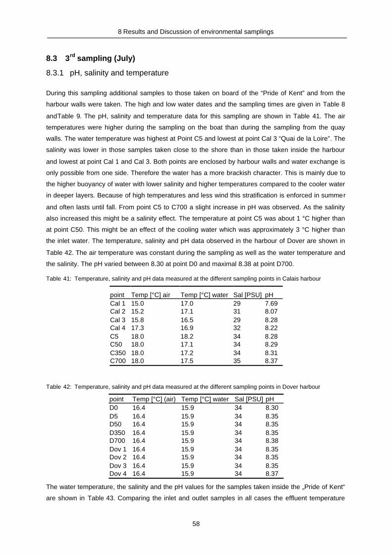
8 Results and Discussion of environmental samplings
58
8.3 3rd sampling (July)
8.3.1 pH, salinity and temperature
During this sampling additional samples to those taken on board of the “Pride of Kent” and from the
harbour walls were taken. The high and low water dates and the sampling times are given in Table 8
andTable 9. The pH, salinity and temperature data for this sampling are shown in Table 41. The air
temperatures were higher during the sampling on the boat than during the sampling from the quay
walls. The water temperature was highest at Point C5 and lowest at point Cal 3 “Quai de la Loire”. The
salinity was lower in those samples taken close to the shore than in those taken inside the harbour
and lowest at point Cal 1 and Cal 3. Both points are enclosed by harbour walls and water exchange is
only possible from one side. Therefore the water has a more brackish character. This is mainly due to
the higher buoyancy of water with lower salinity and higher temperatures compared to the cooler water
in deeper layers. Because of high temperatures and less wind this stratification is enforced in summer
and often lasts until fall. From point C5 to C700 a slight increase in pH was observed. As the salinity
also increased this might be a salinity effect. The temperature at point C5 was about 1 °C higher than
at point C50. This might be an effect of the cooling water which was approximately 3 °C higher than
the inlet water. The temperature, salinity and pH data observed in the harbour of Dover are shown in
Table 42. The air temperature was constant during the sampling as well as the water temperature and
the salinity. The pH varied between 8.30 at point D0 and maximal 8.38 at point D700.
Table 41: Temperature, salinity and pH data measured at the different sampling points in Calais harbour
point Temp [°C] air Temp [°C] water Sal [PSU] pHCal 1 15.0 17.0 29 7.69Cal 2 15.2 17.1 31 8.07Cal 3 15.8 16.5 29 8.28Cal 4 17.3 16.9 32 8.22C5 18.0 18.2 34 8.28C50 18.0 17.1 34 8.29C350 18.0 17.2 34 8.31C700 18.0 17.5 35 8.37
Table 42: Temperature, salinity and pH data measured at the different sampling points in Dover harbour
point Temp [°C] (air) Temp [°C] water Sal [PSU] pHD0 16.4 15.9 34 8.30D5 16.4 15.9 34 8.35D50 16.4 15.9 34 8.35D350 16.4 15.9 34 8.35D700 16.4 15.9 34 8.38Dov 1 16.4 15.9 34 8.35Dov 2 16.4 15.9 34 8.35Dov 3 16.4 15.9 34 8.35Dov 4 16.4 15.9 34 8.37
The water temperature, the salinity and the pH values for the samples taken inside the „Pride of Kent“
are shown in Table 43. Comparing the inlet and outlet samples in all cases the effluent temperature
This document, and more, is available for download at Martin's Marine Engineering Page - www.dieselduck.net

8 Results and Discussion of environmental samplings
59
was about 3 °C higher than that of the inlet water and the pH was lower by about 1.5 pH units. The
salinity was nearly constant with 35 PSU at all points. Inside the seawater scrubber the lowest pH was
found at point SCH6 behind the Ecosilencer. At the US filter inlet and outlet the pH was already 0.14
pH units higher and in the outlet after dilution with the cooling water the pH was nearly neutral.
Table 43: Seawater scrubber temperatures, salinities and pH data
point Temp [°C] water Sal [PSU] pHSD1 17.8 35.0 8.38SD2 20.7 34.0 6.87SCH1 17.4 35.0 8.44SCH2 20.2 35.0 6.99SCH3 36.7 34.5 3.14SCH5 36.0 35.0 3.13SCH6 37.0 35.0 3.09SC1 18.2 35.0 8.16SC2 20.9 35.0 6.82
8.3.2 Nutrients
Table 44 shows the chlorophyll, seston and nutrient data determined for the samples taken in July. In
Dover only at point D5 the chlorophyll content was high enough to be determined. In Calais the
contents varied between 11.7 µg L-1 and 33.1 µg L-1. The highest content was observed at the berth in
front of the “Pride of Kent”. The seawater scrubber inlet and outlet samples taken in Calais are about
equally concentrated as those taken from the transect sampling points. The chlorophyll contents
determined for the remaining seawater scrubber samples are all within the same order of magnitude.
Nearly all seston contents laid between 50 and 65 mg L -1. Only at point C5 a higher seston content of
86.7 µg L-1 was measured. As at this point the chlorophyll content was high too the seston content
most probably originated from a high plankton abundance. Inside the seawater scrubber system the
highest seston content was measured in the outlet of the US filter. Comparing the inlet and outlet
samples only in Dover an increased seston content was observed in the outlet.
The determined RDP, DOP and TDP concentrations show no significant trend and varied between
0.33 - 5.07 µmol L-1 (RDP) 0.11 - 2.41 µmol L-1 (DOP) and 1.12 -2.96 µmol L-1. The highest RDP value
was measured at point Cal 3. At this point also the nitrate, nitrite, ammonium and silicate
concentrations were high. As no significantly higher seston or chlorophyll contents were determined
for that point it can be stated that at this point an algal bloom started. Comparing the determined
concentrations of both harbours it can be seen that in Calais the DIN and silicate concentrations were
generally higher than those in Dover.
Taking the seawater scrubber system samples into closer view, it can be seen that the highest nitrate
concentration was observed behind the Ecosilencer. According to the high ammonia concentration
determined for the US-filter sample the highest DIN concentration was observed at point SCH5. All
This document, and more, is available for download at Martin's Marine Engineering Page - www.dieselduck.net

8 Results and Discussion of environmental samplings
60
outlet samples showed a higher DIN concentration than the inlet sample. This is mainly due to an
increase in NO2- and NO3
-.
Table 44: Chlorophyll, seston and nutrient concentrations determined for the samples taken in July 2004
samp. point TCHL Seston RDP DOP TDP NO2- NO3
- NH4+ DIN Si(OH)4
[µg L-1] [mg L-1] [µmol L-1] [µmol L-1] [µmol L-1] [µmol L-1] [µmol L-1] [µmol L-1] [µmol L-1] [µmol L-1]Cal1 26.7 47.9 4.60 - - 1.01 6.47 53.20 60.68 26.03Cal2 23.5 59.3 3.13 - - 1.34 6.05 32.88 40.27 16.13Cal3 19.3 49.4 5.07 - - 1.61 6.50 70.72 78.83 60.59Cal4 11.7 54.8 1.37 1.12 2.49 1.12 5.29 19.29 25.70 8.84C5 33.1 86.7 0.93 1.56 2.49 0.78 3.65 15.63 20.07 7.48C50 26.1 63.4 0.57 1.65 2.22 0.83 3.85 16.13 20.81 7.89C350 19.5 64.7 0.77 0.65 1.42 0.82 3.53 16.47 20.82 7.97C700 24.3 55.8 1.12 1.06 2.18 0.80 3.48 16.42 20.70 7.85D5 6.3 42.6 0.33 0.93 1.26 0.12 2.42 3.73 6.27 2.34D50 - 57.2 0.33 2.43 2.76 0.16 2.47 3.73 6.36 5.84D350 - 46.9 0.35 0.80 1.16 0.05 1.92 4.10 6.08 2.29D700 - 54.9 0.35 0.78 1.13 0.16 2.36 3.42 5.94 1.38Dov2 - 55.1 0.33 0.73 1.06 0.12 2.38 4.63 7.13 3.62Dov4 - 57.8 1.98 0.11 2.09 0.05 2.34 3.42 5.81 9.12SD1 7.7 74.3 3.04 - - 0.15 3.02 3.64 6.81 4.46SD2 3.7 115.5 1.01 1.28 2.29 1.39 7.70 3.54 12.63 2.45SCH1 2.1 51.4 1.83 0.35 2.18 0.04 1.33 2.88 4.25 3.82SCH2 1.8 51.6 1.37 1.60 2.96 0.63 4.37 0.75 5.75 1.18SCH3 2.5 145.9 1.28 1.10 2.38 0.03 17.25 5.55 22.83 9.48SCH5 0.7 504.6 1.89 0.62 2.51 0.34 16.60 14.85 31.79 17.05SCH6 1.7 73.2 0.42 0.70 1.12 0.33 16.83 8.60 25.75 5.34SC1 14.7 59.8 0.35 2.41 2.76 0.42 2.79 7.20 10.42 3.60SC2 12.4 56.7 0.33 1.82 2.15 2.99 4.05 7.17 14.21 5.19
This document, and more, is available for download at Martin's Marine Engineering Page - www.dieselduck.net

8 Results and Discussion of environmental samplings
61
8.3.3 Polycyclic aromatic hydrocarbons
The PAH contents determined for the samples taken in Calais harbour on July 13th are shown in Table
70. Additionally the sum of the particulate and dissolved fraction is shown in Table 69. The highest
total amount was observed at Point Cal 1 (Quai en eau profonde), the lowest was determined for the
sample taken at the harbour entrance. Observed total amounts were between 46 ng L-1 and 69 ng L-1
and show only little variation. In all samples phenanthrene, fluoranthene and pyrene were the
dominating compounds. High molecular weight PAHs were at almost all locations below the limit of
detection.
The PAH contents determined for the samples taken in Dover are also shown in Table 70. The lowest
contents were determined for the samples taken at Point D 5 and D50 and the highest contents were
detected in the samples taken at point D 350 and point Dov 4. With exception of point D 350 almost no
PAHs bound to particles were found and therefore no high molecular weight PAHs were present. The
dominating component in all cases was phenanthrene. At some locations fluoranthene, pyrene and
chrysene also were found .
The PAH contents determined for the samples taken from the seawater scrubber system are shown in
Table 72. Comparing the inlet and outlet samples, the inlet samples always show very low contents.
These were equally concentrated in Calais and the Channel and had lower contents in Dover.
However the outlet samples show about 40 to 80 times higher total PAH contents than the inlet
samples, but nevertheless 10 times lower than inside the system before the dilution with the cooling
water. The total PAH amount behind the Ecosilencer and behind the US filter are nearly the same,
whereas the sample behind the cyclone shows a lower content. The major differences are due to the
phenanthrene, pyrene and fluoranthene contents.
Quality of measurement: Comparison 1st and 2nd extraction
Fig. 31 shows the results of the regression between the first and the second extraction. On the left the
regression of the extracted material weight is shown. For this determination the filter which was used
for the extraction of the particulate material was weighed before and after the extraction. Before the
latter the filter was dried at 100 °C. The weight thus determined is not comparable to the total
suspended material, because the filter was extracted and is therefore reduced in organic material, but
it can be used to compare the amounts of extracted material between the first and the second
extraction. On the right of Fig. 31 the regression of every single PAH compound of every single
sample determined during the first extraction was plotted against those from the second extraction.
In both regressions the slope and the R² should be, in the best case, 1. This would show that for both
cases the amount of extracted material was the same and that in both extractions the same PAH
contents were measured. Due to the accuracy of the method (chapter 4.2) the R² and the slope might
vary. As can be seen the difference is smaller than 4 % and therefore within the statistical range.
This document, and more, is available for download at Martin's Marine Engineering Page - www.dieselduck.net

8 Results and Discussion of environmental samplings
62
y = 0,9847xR2 = 0,9785
0,000
0,005
0,010
0,015
0,020
0,025
0,030
0,035
0,040
0,000 0,005 0,010 0,015 0,020 0,025 0,030 0,035 0,040
1st extraction
2nd
extr
actio
n
y = 1,0397xR2 = 0,9632
0
1000
2000
3000
4000
5000
6000
7000
8000
9000
0 1000 2000 3000 4000 5000 6000 7000 8000 9000
1st extraction
2nd
extr
act
ion
Fig. 31: Regression between 1st and 2nd extraction. Left: Regression of the amount of extracted particulatematerial [g]. Right: Regression of all PAHs [ng/L] (sum particulate, dissolved).
Origin of PAHs
In Fig. 32 the isomeric ratios of phenantrene/anthracene and fluoranthene/pyrene of the harbour
samples and the seawater scrubber samples are shown. The Calais harbour samples show a
behaviour similar to the harbour samples taken in February and March and are situated between a
petrogenic and a pyrolytic origin. In contrast the samples taken in Dover seem to originate from a
petrogenic pollution source.
Thehe Ecosilencer samples also show a comparable pattern. The PAHs from the sample behind the
Ecosilencer and from those before and behind the US filter have high phenanthrene to anthracene
ratios and low fluoranthene to pyrene ratios and are therefore most likely of petrogenic origin. The
PAHs in the outlet samples seem to be of petrogenic origin but not as markedly as the undiluted
samples. The inlet samples are comparable to the harbour samples.
0
10
20
30
40
50
60
70
0,0 0,2 0,4 0,6 0,8 1,0 1,2 1,4 1,6
flu/pyr
phe/
ant
CalaisDover
petrogenic
pyrolyticcoal tar
shale oil
0
10
20
30
40
50
60
70
0,0 0,2 0,4 0,6 0,8 1,0 1,2 1,4 1,6
flu/pyr
phe
/an
t
petrogenic
pyrolyticcoal tar
shale oil
P26 outlet ES
P23 outlet US
P25 inlet US
P12 SWS outlet Dover
P22 SWS outlet Channel
P32 SWS outlet Calais
P31 SWS inlet Calais
P21 SWS inletChannelP11 SWS inlet Dover
Fig. 32: Plot of isomeric phenanthrene/anthracene ratios against fluoranthene/pyrene ratios for all harboursamples (left) and seawater scrubber samples (right).
The ratios of benz[a]anthracene and chrysene, which can also be used to determine the origin of the
PAHs in the samples are shown in Table 45. It can be seen that in most cases the contents of the two
compounds were too low and therefore this index could not be used to determine the origin. Only the
This document, and more, is available for download at Martin's Marine Engineering Page - www.dieselduck.net

8 Results and Discussion of environmental samplings
63
contents of the outlet and the seawater scrubber samples were high enough. The quotients of these
samples are greater than one and therefore indicate pyrolytic origin.
Table 45: Quotient of benz[a]anthracene and chrysene.
sampl.point Cal 1 Cal 2 Cal 3 Cal 4 C5 C50 C350 C700
BaA/CHRY 1.00 0.00 - - 1.00 - - -
sampl.point Dov 2 Dov 3 Dov 4 D5 D50 D350 D700
BaA/CHRY - - - - - 0.20 -
sampl.point SD1 SD2 SCH1 SCH2 SC1 SC2 SCH3 SCH5 SCH6
BaA/CHRY 0.00 1.89 0.00 1.47 0.00 1.86 2.63 2.46 2.26
Table 46: Regression of PAH components, yellow shows high correlation
AT
HY
AT
HE
FLR
E
PH
EN
AN
TH
FLU
A
PY
R
BaA
CH
RY
Bbk
F
BaP
Dah
A
Bgh
iP
IND
E
ATHY 1 0.951 0.965 0.932 0.925 0.939 0.922 0.927 0.901 0.939 0.942 0.936 0.94 0.935ATHE 1 0.979 0.98 0.957 0.982 0.967 0.972 0.943 0.984 0.992 0.978 0.986 0.983FLRE 1 0.993 0.991 0.994 0.984 0.987 0.976 0.987 0.994 0.981 0.988 0.99PHEN 1 0.99 0.999 0.996 0.998 0.99 0.991 0.993 0.979 0.988 0.976ANTH 1 0.991 0.986 0.989 0.989 0.979 0.98 0.973 0.977 0.971FLUA 1 0.994 0.998 0.988 0.993 0.994 0.982 0.99 0.98PYR 1 0.995 0.994 0.977 0.981 0.959 0.972 0.959BaA 1 0.992 0.991 0.989 0.979 0.987 0.97CHRY 1 0.969 0.947 0.951 0.962 0.943BbkF 1 0.996 0.996 0.999 0.986BaP 1 0.99 0.997 0.993DahA 1 0.998 0.988BghiP 1 0.991INDE 1
To examine whether the PAHs inside the harbour originate from one source the regression
coefficients for the linear regression of the compounds were calculated. These calculations might
show, whether the composition of the 16 EPA PAHs are comparable among each other. The results
are shown in Table 46. It can be seen that all compounds are highly correlated. As many PAHs had
values lower than the detection limit and some like phenanthrene appeared in high contents, the
results might only “pretend” a high correlation. Therefore the R² was calculated for the linear
regression of each station with the remaining stations. The results are shown in Table 47. It can be
seen that sample Cal 3 does not correlate with any other sample, and that the samples taken from the
seawater scrubber are only moderately correlated with the harbour samples. However the harbour
samples and the inlet samples with exception of the Channel inlet sample also show a good
correlation aa do the SWS samples among each other. In summary it can be said that the harbour
samples and the seawater scrubber inlet samples show a similar PAH composition. The seawater
This document, and more, is available for download at Martin's Marine Engineering Page - www.dieselduck.net

8 Results and Discussion of environmental samplings
64
scrubber samples make up another group which is not even comparable to the samples taken directly
in front of the outlet of the “Pride of Kent”. The PAH composition of point Cal 3 is totally different from
the remaining samples.
Table 47: Regression of sampling points. Colours are added for a better visualisation. Yellow - highly correlated,orange and red moderate or low correlation, dark red - no significant correlation.
Cal 1 Cal 2 Cal 3 Cal 4 C05 C50 C350 C700 D05 D50 D350 D700 Dov2 Dov4 SD1 SD2 SCH1 SCH2 SCH3 SCH5 SCH6 SC1 SC2Cal 1 1 0.892 0.638 0.832 0.918 0.887 0.864 0.743 0.61 0.675 0.858 0.83 0.868 0.883 0.836 0.662 0.743 0.598 0.624 0.646 0.643 0.821 0.614 Cal 1Cal 2 1 0.506 0.877 0.916 0.912 0.951 0.877 0.77 0.788 0.895 0.889 0.891 0.953 0.875 0.713 0.807 0.657 0.663 0.685 0.682 0.897 0.641 Cal 2Cal 3 1 0.492 0.505 0.429 0.431 0.255 0.146 0.158 0.402 0.335 0.36 0.388 0.38 0.146 0.262 0.104 0.126 0.139 0.144 0.339 0.152 Cal 3Cal 4 1 0.759 0.791 0.85 0.789 0.733 0.746 0.713 0.845 0.909 0.864 0.723 0.644 0.804 0.584 0.604 0.621 0.613 0.752 0.557 Cal 4C05 1 0.89 0.881 0.789 0.672 0.722 0.892 0.824 0.836 0.911 0.836 0.707 0.708 0.646 0.671 0.689 0.687 0.844 0.654 C05C50 1 0.952 0.932 0.829 0.864 0.858 0.964 0.906 0.957 0.948 0.75 0.825 0.69 0.702 0.728 0.716 0.924 0.659 C50C350 1 0.95 0.836 0.872 0.821 0.959 0.921 0.957 0.891 0.738 0.843 0.682 0.692 0.715 0.702 0.899 0.644 C350C700 1 0.934 0.946 0.779 0.975 0.91 0.93 0.888 0.793 0.866 0.752 0.751 0.772 0.752 0.893 0.677 C700D05 1 0.976 0.702 0.908 0.832 0.856 0.8 0.821 0.843 0.775 0.778 0.796 0.779 0.852 0.693 D05D50 1 0.738 0.94 0.88 0.892 0.834 0.851 0.883 0.811 0.807 0.825 0.808 0.882 0.723 D50D350 1 0.812 0.807 0.863 0.913 0.799 0.81 0.764 0.753 0.773 0.776 0.931 0.764 D350D700 1 0.949 0.947 0.926 0.802 0.912 0.754 0.757 0.78 0.762 0.924 0.694 D700Dov 2 1 0.943 0.847 0.833 0.879 0.789 0.804 0.819 0.807 0.861 0.749 Dov 2Dov 4 1 0.881 0.778 0.822 0.714 0.731 0.752 0.743 0.903 0.676 Dov 4SD1 1 0.781 0.897 0.751 0.726 0.752 0.746 0.977 0.715 SD1SD2 1 0.82 0.988 0.993 0.996 0.996 0.836 0.972 SD2SCH1 1 0.81 0.768 0.7889 0.78 0.924 0.738 SCH1SCH2 1 0.984 0.985 0.985 0.805 0.973 SCH2SCH3 1 0.999 0.997 0.78 0.978 SCH3SCH5 1 0.998 0.805 0.976 SCH5SCH6 1 0.803 0.986 SCH6SC1 1 0.769 SC1SC2 1 SC2
Principal component analysis
In Fig. 33 and in Table 48 the results of the PCA of all harbour samples and the SWS inlet samples
taken in July are given. In this case eigenvector 1 accounts for 33.6 % and eigenvector 2 for19.7 % of
the total variance. As both vectors only make up 52.3 % of the total variance only a part of the total
variability within these samples can be explained. According to the PCA plot the samples can be
divided into three groups. The first one is made up by C 50, C700, D 5, D 50, D 700, Dov 2, SD1 and
SC1. These samples are all in the third quadrant meaning they are negative on both axes. Looking at
the feature vector this indicates low overall concentrations and especially low anthracene, pyrene and
fluoranthene concentrations. The second group is made up by the samples Cal 2, Cal 3, Cal 4, C 350
and Dov 4. These are in the second quadrant meaning they are positively related to eigenvector 2 and
negatively related to eigenvector. As eigenvector 1 is mainly positive, this indicates, that the samples
of this group have higher contents the more they are situated on the positive side. The third group is
made up by Cal 1, C 5 and D 350. These samples also showed the highest overall concentrat ion. The
pattern that is drawn in Fig. 33 is nearly the same, which can be observed in the regression chart
(Table 47). Cal 3, Cal 1, C5 and D350 are separated and have only low correlations with the
remaining points, whereas the remaining points are higher correlated.
This document, and more, is available for download at Martin's Marine Engineering Page - www.dieselduck.net
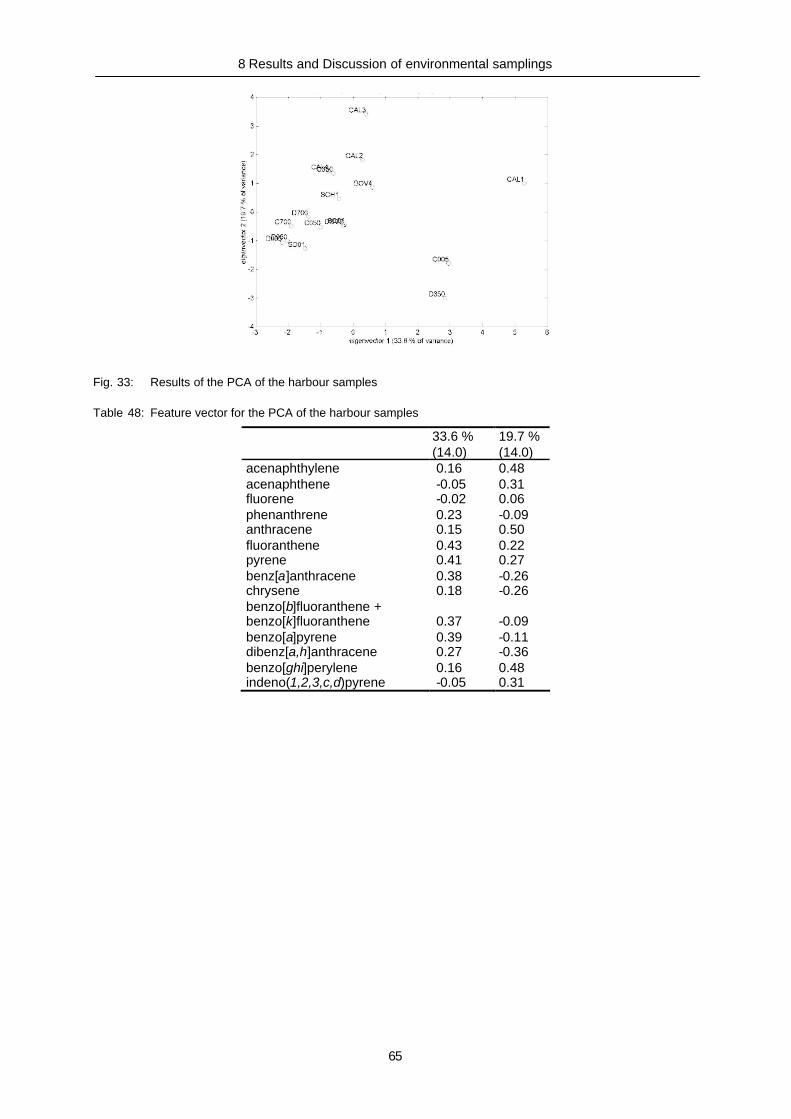
8 Results and Discussion of environmental samplings
65
Fig. 33: Results of the PCA of the harbour samples
Table 48: Feature vector for the PCA of the harbour samples
33.6 %(14.0)
19.7 %(14.0)
acenaphthylene 0.16 0.48acenaphthene -0.05 0.31fluorene -0.02 0.06phenanthrene 0.23 -0.09anthracene 0.15 0.50fluoranthene 0.43 0.22pyrene 0.41 0.27benz[a]anthracene 0.38 -0.26chrysene 0.18 -0.26benzo[b]fluoranthene +benzo[k]fluoranthene 0.37 -0.09benzo[a]pyrene 0.39 -0.11dibenz[a,h]anthracene 0.27 -0.36benzo[ghi]perylene 0.16 0.48indeno(1,2,3,c,d)pyrene -0.05 0.31
This document, and more, is available for download at Martin's Marine Engineering Page - www.dieselduck.net

8 Results and Discussion of environmental samplings
66
8.4 4th sampling (September)
8.4.1 pH, salinity and temperature
The date and time when the samples were taken during the fourth sampling are given in Table 9. The
high and low water times are shown in Table 8. It can be seen that in Calais the samples were taken
during high tide and three hours after high tide. In Dover the samples were taken approximately one
hour after ebb tide.
The pH, salinity, air and water temperatures are shown in Table 49 (Calais), Table 50 (Dover) and in
Table 51 (seawater scrubber). The air temperatures during the sampling from the quay walls in Calais
varied between 19.0 and 19.5 °C and the water temperature between 21.5 and 22.1 °C. During the
sampling from the small boat at point C0, C5, C50, C350, C700 the air temperature was about 3 to
4 °C higher. The water temperature at point C5 and C50 was slightly increased (0.5 °C) whereas the
remaining points had about the same water temperature as the samples taken from the harbour walls.
The increase in temperature might be an effect of the seawater scrubber effluent.
Table 49: Temperature, salinity and pH data measured at the different sampling points in Calais harbour inSeptember
Point Temp [°C]air
Temp [°C]water Sal [PSU] pH
Cal 1 19.5 22.1 34.1 7.95Cal 2 19.5 22.1 34.0 7.97Cal 3 19.0 21.5 31.9 7.89Cal 4 19.1 21.9 33.7 8.04C 0 22.3 23.3 34.3 8.08C 5 23.5 23.1 34.6 8.08C 50 23.0 22.8 34.7 8.09C 350 22.2 22.8 34.7 8.09C 700 22.2 22.9 34.6 8.10
Table 50: Temperature, salinity and pH data measured at the different sampling points in Dover harbour inSeptember
Point Temp [°C]air
Temp [°C]water Sal [PSU] pH
D 5 26.9 22.8 35.1 8.07D 50 24.4 22.3 35.2 8.04D 350 25.1 22.1 35.0 8.05D 700 23.6 22.1 35.0 8.04Dov 1 23.3 22.2 35.0 8.07Dov 2 22.6 22.2 35.1 8.08Dov 3 22.6 21.9 35.1 8.08Dov 4 25.0 22.2 35.2 8.08
This document, and more, is available for download at Martin's Marine Engineering Page - www.dieselduck.net

8 Results and Discussion of environmental samplings
67
Table 31 shows that the seawater scrubber outlet water was 13 to 17 °C warmer than the inlet water.
This difference is more than 10 °C higher than those observed during the first three samples. An
increased temperature was also observed at the first and second points in Dover in a distance of 5
and 50 m away from the outlet. At point D 5 the temperature was 0.7 °C higher than at the remaining
points inside the harbour, with the exception of point Dov 3 in the middle of the port, where the
temperature was the lowest (21.9 °C). Inside the seawater scrubber system the highest temperatures
were measured directly after the Ecosilencer, in front of and behind the US-filter. Here the
temperatures were 45.1, 45.3 and 46.2 °C, respectively. The water in the seawater scrubber outlet still
had a temperature of 35.7, 37.1 and 37.6 °C. The pH inside the harbour was nearly constant for all
samples with exception of the samples taken from the quay walls in Calais. Inside the seawater
scrubber system the lowest pH (3.05) was determined in the pipe leading to the settling tank and also
behind the US filter. The outlet water in Dover, the Channel and Calais showed a pH of 6.2, 6.4 and
6.15, respectively. It was about 1.7 pH units lower in comparison to the inlet water. The samples taken
inside the Channel had a salinity of about 37 whereas in Calais and Dover the salinity varied between
34 and 35. At point Cal 3 a salinity of only 31.9 was observed due to the enclosed situation of that
sampling point.
Table 51: Temperature, salinity and pH data measured at the different sampling points in the seawater scrubberin September
Point Temp [°C]water Sal [PSU] pH
SD1 24.0 34.4 7.99SD2 37.6 35.7 6.20SCH1 23.0 36.0 8.08SCH2 37.1 36.0 6.40SCH3 45.3 36.8 3.14SCH4 42.5 36.6 3.05SCH5 46.2 36.8 3.05SCH6 45.1 36.4 3.13SCH7 38.5 37.0 3.04SC1 20.7 34.5 7.88SC2 37.6 34.7 6.15
This document, and more, is available for download at Martin's Marine Engineering Page - www.dieselduck.net

8 Results and Discussion of environmental samplings
68
8.4.2 Nutrients
The chlorophyll, seston and nutrient concentrations determined for the samples taken in September
are shown in Table 52. It can be seen that in Dover the chlorophyll concentration was generally lower
than in Calais. The highest chlorophyll content was measured at point Cal 3 (181.9 µg L -1). At this
point also the highest seston, silicate, ammonium and RDP concentrations ws determined, whereas
the nitrate concentration was the lowest observed in all samples. This shows that there was an algal
bloom at this point. The nitrate concentration was reduced because it is used as an important nitrogen
supply. Ammonium is the first degradation product of nitrogen-containing organic material. Hence the
higher concentrations in the harbour waters of Calais indicate that somde degradation already had
taken place. At the remaining points in Calais the chlorophyll concentrations varied between 5.1 and
48.4 µg L-1. The lowest value was observed at point Cal 1 and the highest at C350. In Dover
Chlorophyll concentration between 4.2 (Dov 4) and 12.8 µg L-1 (D350) were observed. The RDP,
DOP, TDP, seston and silicate values were all within the same range as in Calais, whereas the nitrate
concentrations were increased and the ammonium concentrations were lower in Dover. Taking a look
at the first transect samples D5 and C5 it can be seen that the nitrate concentrations are slightly
increased in comparison to the other points. This could be an effect of the seawater scrubber but also
of eutrophication due to the enclosed area and the ship traffic.
Table 52: Chlorophyll, seston and nutrient concentrations determined for the samples taken in September 2004
samp.point
TCHL Seston RDP DOP TDP NO3- NH4
+ DIN Si(OH)4
[µg L-1] [mg L-1] [µmol L-1] [µmol L -1] [µmol L-1] [µmol L-1] [µmol L -1] [µmol L-1] [µmol L-1]Cal1 5.1 54.8 0.87 0.13 1.00 4.05 12.60 17.29 7.82Cal2 16.2 56.7 0.97 0.07 1.04 3.76 14.20 18.60 8.57Cal3 181.9 100.8 4.50 0.31 4.81 0.75 41.93 43.19 14.73Cal4 22.9 64.0 0.65 0.31 0.96 3.52 9.28 13.36 6.92C0 23.2 86.0 0.47 0.52 0.99 2.79 8.28 11.59 6.83C5 35.3 76.2 0.39 0.61 0.99 3.58 9.95 14.02 6.84C50 43.2 89.2 0.37 0.56 0.94 2.78 7.93 11.19 6.64C350 48.4 76.5 0.37 0.19 0.56 2.52 9.02 12.02 5.04C700 44.9 67.3 0.23 0.50 0.73 2.86 8.14 11.47 4.15D5 7.2 59.5 0.55 0.35 0.90 2.86 0.63 3.80 6.78D50 10.5 59.7 0.65 0.06 0.70 2.50 1.50 4.31 6.46D350 12.8 58.8 0.23 0.24 0.47 2.58 1.44 4.31 4.94D700 10.0 72.6 0.19 0.13 0.32 4.33 0.34 5.06 5.00Dov1 5.9 74.8 0.55 0.23 0.78 7.37 1.22 9.07 6.02Dov2 9.9 61.3 0.44 0.09 0.53 5.43 1.38 7.29 5.00Dov3 7.6 65.6 0.44 0.08 0.52 5.32 1.41 7.19 6.49Dov4 4.2 66.0 0.21 0.03 0.24 4.27 1.78 6.35 6.02SD1 16.5 62.1 0.23 0.09 0.32 3.63 1.43 5.39 6.81SD2 9.6 69.9 0.22 0.08 0.30 7.66 2.42 10.79 6.00SCH1 5.7 57.8 0.20 0.09 0.29 3.96 2.26 6.63 3.89SCH2 6.1 55.0 0.20 0.03 0.23 3.77 2.08 6.27 3.15SCH3 10.2 54.1 0.78 0.29 1.07 19.21 4.33 23.61 7.58SCH4 9.6 70.6 1.35 0.23 1.59 21.58 8.40 30.61 12.31SCH5 6.7 61.1 0.83 0.10 0.93 18.27 3.67 22.01 6.95SCH6 4.6 57.6 0.99 0.09 1.08 17.85 3.40 21.32 10.04SCH7 7.4 99.1 1.54 0.08 1.62 21.05 4.90 26.10 12.28SC1 49.1 61.8 0.64 0.15 0.79 3.76 8.33 12.63 8.70SC2 32.0 64.2 0.42 0.23 0.65 5.52 7.37 13.54 7.60
Looking at the seawater scrubber inlet and outlet samples it can be seen that the nitrate
concentrations are higher in the outlet, in Calais they even doubled. On board, the highest nitrate
concentrations were not observed directly behind the Ecosilencer but at point SCH4, the pipe leading
This document, and more, is available for download at Martin's Marine Engineering Page - www.dieselduck.net

8 Results and Discussion of environmental samplings
69
to the settling tank, and at point SCH7, the settling tank. These points also show high TDP, silicate
and seston values. As silicate is the main substance of which diatom tests are built up it is not
surprising that it is enriched by the cyclones in the seawater scrubber system. Comparing the inlet and
outlet samples it can be seen that the nitrate concentration due to the formation of nitric acid in the
Ecosilencer is increased. Additional ly the seston content is higher in the outlet samples. This might
result from remaining soot particles originating from the scrubbing process.
8.4.3 Metals and Sulphate
Table 53 shows the sulphate, earth and transition metal concentrations determined for the samples
taken in Dover and Calais directly in front of the seawater scrubber outlet and inside the seawater
scrubber system. It can be seen that As, Ba, Cd, Co, Cr, Cu, Mn, Mo, Ni, Pb could not be detected. Fe
was only found inside the seawater scrubber system but not in the inlet and the outlet. The highest
iron content (4513 ppb) was found at point SCH4 in the pipe leading to the settling tank. One reason is
the very low pH measured at this point which increases the solubility of iron. Another reason is that all
particles collected in the seawater scrubber system, which also contain rust, are concentrated in the
cyclones and pass this pipe, and a third aspect might be an overflow pipe from the funnel which flows
into the settling tank pipe shortly before point SCH4 and which might contain particles and rust from
the funnel. The same reasons might be responsible for the high vanadium concentration measured at
point SCH4. However K, Li and Mg have nearly constantly contents in all samples, whereas the
strontium concentration is higher in Calais than in Dover.
Table 53: Sulphate, earth and transition metals determined for the samples taken in September ( - belowdetection limit)
SD 1 SD2 SCH1 SCH2 SCH3 SCH4 SCH5 SCH6 SC2 SC 1As ppb - - - - - - - - - -Ba ppb - - - - - - - - - -Ca ppm 393 397 383 386 404 407 404 411 411 389Cd ppb - - - - - - - - - -Co ppb - - - - - - - - - -Cr ppb - - - - - - - - - -Cu ppb - - - - - - - - - -Fe ppb - - - - 803 4513 687 680 - -K ppm 380 380 390 340 360 400 400 380 370 330Li ppb 180 180 170 180 180 180 180 180 180 180Mg ppm 1235 1230 1205 1205 1260 1265 1255 1290 1265 1220Mn ppb - - - - - - - - - -Mo ppb - - - - - - - - - -Ni ppb - - - - - - - - - -Pb ppb - - - - - - - - - -SO4 ppm 2670 2710 2590 2600 2940 2940 2990 2980 2870 2590Sr ppb 7680 7760 7515 7705 7915 7915 8020 8055 8035 7620V ppb - - - - 155 420 240 170 - -Zn ppb - 290 - - 455 - 395 360 - -
Zinc was only determined in the outlet sample in Dover and at points SCH3, SCH5 and SCH6, but not
in the pipe going to the settling tank and in no other outlet sample. The source for this contamination
This document, and more, is available for download at Martin's Marine Engineering Page - www.dieselduck.net

8 Results and Discussion of environmental samplings
70
might be the valves used during the sampling which might contain zinc. Otherwise if zinc would
originate from the system itself it should also have been detected at point SCH4 and in the outlet
water.
As expected the sulphate concentration was increased inside the seawater scrubber due to the
formation of sulphuric acid, but comparing the in and outlet sample taken in the Channel no increase
was observed.
Summarising the data of Table 53 it can be said that no increase in the metal or sulphate
concentration was observed outside the “Pride of Kent” and that the increased Fe and V
concentrations were only observed inside the pipe leading to the settling tank. As the water and the
particles from the settling tank will be treated in a special way (deposition or burning), and as Fe and V
are not toxic, no negative effect is to be expected.
8.4.4 Polycyclic aromatic hydrocarbons
The concentrations of the determined dissolved and particle bound PAHs are shown in Table 70 and
Table 72.The total amounts of all EPA PAHs (without naphthalene) are given in Table 69. Comparing
the total amounts with the samplings in February, March and July, it can be seen that the contents in
September were especially in Calais about 100 ng L-1 higher than in July, but the overall
concentrations where not as high as in March or February. All analysed concentrations were situated
between 44 and 248 ng L-1 with exception of the outlet samples where concentrations of 3422, 3263
and 3577 ng L-1 were determined. Taking a closer view at the single compounds it can be seen that
almost no acenaphthene, acenaphthylene, anthracene, benzo[b+k]fluoranthene, benz[a]pyrene,
dibenz[a,h]anthracene, benzo[ghi]perylene or indeno[1,2,3,c,d]pyrene were present. In all samples
phenanthrene, fluoranthene and pyrene dominated. These three compounds as well as fluorene were
also the dominating compounds in the seawater scrubber effluent, where phenanthrene
concentrations of 1400 ng L-1 were detected. No increased contents of high molecular weight PAHs
were found in the outlet samples.
Looking at the PAH concentration determined 5, 50, 350 and 700 m away from the seawater scrubber
outlet no increase was observed. In contrary the transect samples taken in Calais show lower PAH
concentrations than the samples taken from the quay walls. Additionally the blank sample taken
before the “Pride of Kent” arrived showed a higher PAH concentration (133 ng L-1) than the sample
taken at point C 5 (109 ng L-1). In Dover the sample taken 5 m away from the outlet had a content
similar to the sample from the middle port at point Dov 2. All these observations show that the
seawater scrubber effluent does not seem to increase the PAH concentration.
Inside the seawater scrubber all four- and five-ring compounds with the exception of fluoranthene and
pyrene were nearly completely found bound to the particulate fraction. Phenanthrene which partially
made up about 50 % of the total amount of all measured PAHs was also found in high concentrations
This document, and more, is available for download at Martin's Marine Engineering Page - www.dieselduck.net

8 Results and Discussion of environmental samplings
71
in the particulate fraction. This shows that most of the PAHs are bound to soot particles, and that an
effective remove of these particles is able to lower these concentrations significantly.
Quality of measurement: Comparison 1st and 2nd extraction
Fig. 34 shows the regression of the extracted and dried filters and of the determined PAHs (chapter
8.3.3). In both cases high correlation coefficients and slopes close to one were observed. Therefore
the results of the first and the second extraction are very similar.
y = 1,0323xR2 = 0,9702
0,000
0,005
0,010
0,015
0,000 0,005 0,010 0,015
1st extraction
2nd
extr
acti
on
y = 0,9533xR2 = 0,9707
0
2000
4000
6000
8000
10000
0 5000 10000
1st extraction
2ndex
trac
tion
Fig. 34: Regression between 1st and 2nd extraction left: Regression between the amount of extracted particulatematerial [g]. Right: Regression of all determined PAH concentrations [ng/l] (sum, particulate,dissolved).
Origin of PAHS
To determine the origin of the PAHs a regression of the compound concentrations among each other
and a regression of the concentrations determined at the single sampling points was performed. The
results are shown in Table 55 and Table 54.
The correlation coefficients of Table 54 show high correlation coefficients for nearly all compounds.
When a high correlation between for example fluoranthene and pyrene was found this meant that at all
points where high concentrations of fluoranthene were measured, also high concentrations of
phenanthrene were measured. If the relative relations of all compounds were the same at all points,
and differences only appear in the concentration itself, high correlation coefficients would be observed
for all compounds. As the anthracene concentrations were often close to or lower than the detection
limit, the R² for the correlation with this compound is low. The same reason can be given for the low R²
observed for the correlations with dibenz[ah]anthracene and acenaphthylene. As this method of
regression analysis is not very specific and gives no information about the similarity of single sampling
points, a regression of the observed PAH concentrations of the sampling points was also performed.
This document, and more, is available for download at Martin's Marine Engineering Page - www.dieselduck.net

8 Results and Discussion of environmental samplings
72
Table 54: Regression of compounds. Colours are added for a better visualisation. Yellow - highly correlated, darkred - no significant correlation.
AT
HY
AT
HE
FL
RE
PH
EN
AN
TH
FL
UA
PY
R
BaA
CH
RY
Bbk
F
BaP
Dah
A
Bgh
iP
IND
E
ATHY 1 0.787 0.819 0.851 0.619 0.876 0.874 0.851 0.891 0.93 0.759 0.921 0.941 0.934ATHE 1 0.994 0.988 0.927 0.976 0.978 0.974 0.966 0.7 0.948 0.824 0.753 0.815FLRE 1 0.997 0.918 0.99 0.991 0.987 0.982 0.74 0.959 0.851 0.79 0.843PHEN 1 0.895 0.996 0.998 0.991 0.992 0.778 0.952 0.878 0.823 0.872ANTH 1 0.872 0.873 0.9 0.855 0.487 0.952 0.608 0.548 0.601FLUA 1 0.999 0.989 0.996 0.815 0.942 0.899 0.856 0.896PYR 1 0.991 0.997 0.811 0.943 0.898 0.852 0.894BaA 1 0.993 0.769 0.974 0.848 0.805 0.843CHRY 1 0.831 0.943 0.902 0.863 0.899BbkF 1 0.645 0.956 0.99 0.965BaP 1 0.728 0.689 0.722DahA 1 0.97 0.997BghiP 1 0.981INDE 1
Table 55: Regression of sampling points. Colours are added for a better visualisation. Yellow highly correlated,orange and red moderate or low correlation, dark red no significant correlation.
Cal1 Cal2 Cal3 Cal4 C0 C5 C50 C350 C700 D5 D50 D350 D700 Dov2 Dov3 Dov4 SD1 SD2 SCH1 SCH2 SCH3 SCH4 SCH5 SCH6 SC1 SC2Cal1 1 0,926 0,837 0,835 0,914 0,957 0,893 0,942 0,935 0,791 0,918 0,675 0,628 0,982 0,801 0,715 0,929 0,785 0,769 0,743 0,761 0,731 0,752 0,771 0,811 0,768 Cal1Cal2 1 0,745 0,824 0,878 0,940 0,839 0,934 0,859 0,782 0,840 0,575 0,502 0,893 0,753 0,599 0,827 0,754 0,683 0,701 0,733 0,738 0,727 0,731 0,727 0,740 Cal2Cal3 1 0,852 0,889 0,815 0,936 0,758 0,781 0,877 0,896 0,865 0,843 0,830 0,881 0,931 0,886 0,893 0,931 0,882 0,882 0,837 0,868 0,898 0,917 0,884 Cal3Cal4 1 0,968 0,817 0,958 0,757 0,778 0,977 0,795 0,866 0,769 0,802 0,975 0,822 0,896 0,947 0,908 0,919 0,941 0,930 0,945 0,936 0,950 0,943 Cal4C0 1 0,904 0,974 0,856 0,879 0,932 0,855 0,818 0,740 0,872 0,946 0,816 0,915 0,900 0,877 0,865 0,882 0,858 0,880 0,889 0,930 0,892 C0C5 1 0,858 0,972 0,945 0,775 0,914 0,616 0,585 0,905 0,770 0,650 0,834 0,765 0,735 0,719 0,737 0,712 0,730 0,749 0,779 0,745 C5C50 1 0,811 0,877 0,948 0,879 0,886 0,810 0,882 0,971 0,900 0,943 0,938 0,935 0,913 0,917 0,882 0,924 0,931 0,958 0,930 C50C350 1 0,917 0,690 0,895 0,520 0,472 0,896 0,697 0,568 0,785 0,675 0,657 0,619 0,645 0,621 0,631 0,654 0,690 0,649 C350C700 1 0,753 0,943 0,679 0,683 0,909 0,783 0,746 0,841 0,766 0,775 0,734 0,743 0,705 0,729 0,758 0,804 0,747 C700D5 1 0,784 0,919 0,929 0,770 0,978 0,878 0,889 0,982 0,944 0,970 0,977 0,964 0,985 0,978 0,970 0,986 D5D50 1 0,711 0,708 0,917 0,795 0,768 0,868 0,827 0,843 0,797 0,801 0,752 0,777 0,819 0,823 0,800 D50D350 1 0,962 0,681 0,939 0,970 0,844 0,937 0,963 0,955 0,936 0,893 0,946 0,949 0,963 0,945 D350D700 1 0,638 0,861 0,947 0,782 0,886 0,925 0,917 0,891 0,841 0,890 0,905 0,917 0,892 D700Dov2 1 0,786 0,733 0,949 0,782 0,768 0,745 0,755 0,721 0,747 0,770 0,793 0,765 Dov2Dov3 1 0,903 0,901 0,966 0,953 0,953 0,953 0,923 0,968 0,963 0,983 0,965 Dov3Dov4 1 0,861 0,904 0,953 0,919 0,897 0,847 0,901 0,919 0,937 0,908 Dov4SD1 1 0,896 0,884 0,874 0,877 0,841 0,879 0,891 0,910 0,890 SD1SD2 1 0,972 0,995 0,991 0,965 0,995 0,999 0,973 0,998 SD2SCH1 1 0,974 0,963 0,913 0,959 0,978 0,979 0,966 SCH1SCH2 1 0,990 0,962 0,994 0,998 0,969 0,996 SCH2SCH3 1 0,988 0,990 0,992 0,966 0,992 SCH3SCH4 1 0,971 0,964 0,928 0,970 SCH4SCH5 1 0,995 0,970 0,999 SCH5SCH6 1 0,976 0,998 SCH6SC1 1 0,972 SC1SC2 1 SC2
Taking Table 55 into closer view, it can be seen that most of the sampling points are highly correlated.
Especially the correlation between the seawater scrubber samples among each other and the Calais
samples among each other showed high R² values indicating that the PAH composition of these
samples is similar. In contrary the correlation of the samples taken from the harbour in Dover seem to
be different in their composition from the samples taken in Calais. They show only moderate
correlation coefficients for these regressions, but high correlation coefficients when compared with the
seawater scrubber samples. The samples taken from the Calais transect are only moderately
correlated with the samples taken from the seawater scrubber. Summarising can be said, that all
Dover samples show a comparable composition while the Calais samples are not comparable to the
seawater scrubber samples. Therefore the composition of the Dover and Calais samples is different
too.
This document, and more, is available for download at Martin's Marine Engineering Page - www.dieselduck.net

8 Results and Discussion of environmental samplings
73
Additionally to the regression analysis a principal component analysis (Fig. 36, Table 57) and an
analysis of the isomeric ratios of phenanthrene to anthracene, fluoranthene to pyrene (Fig. 35) and
benz[a]anthracene to chrysene (Table 55) was performed. The plot of the phen/anth ratios against the
flua/pyr ratios indicates that the seawater scrubber samples seem to originate from a petrogenic
source. This would underline the results of the previous samplings. The same holds for the isomeric
ratios of benz[a]anthracene and chrysene which are all smaller than one and therefore indicate a
pyrolytic origin too.
0
10
20
30
40
50
60
70
80
90
100
0,0 0,5 1,0 1,5 2,0 2,5
phenanthrene / anthracene
flu
ora
then
e/
py
ren
e
DoverCalaisSWSoutlet
petrogenic
pyrolytic
D 350
Fig. 35: Plot of isomeric phenanthrene/anthracene ratios against fluoranthene/pyrene ratios for all samples
The phenanthrene to anthracene ratios of the harbour samples are close to ten and the fluoranthene
to pyrene and the benz[a]anthracene to chrysene ratios are close to one. This might have the same
reasons as those mentioned in the discussion of the February, March and July samplings. The explicit
petrogenic character of the sample D 350, which shows nearly the same isomeric ratios as the outlet
samples cannot be explained. Perhaps a thin oil film flowing on top of the water contaminated this
sample.
The principal component analysis underlines and specifies the results of the regression analysis. From
this the samples can be divided into three different groups. The first group is made up by only one
sample: Cal 2. This sample is characterised by relative high anthracene, fluoranthene and pyrene
contents. As point Cal 2 is situated close to the place where the service boats anchor, these might
originate from the lighter petroleum used for these boats.
Table 56: The quotient of benz[a]anthracene to chrysene can be used as marker for the origin of a sample
sampl. point Cal 1 Cal 2 Cal 3 Cal 4 C0 C5 C50 C350 C700BaA/CHRY 0,2 0,9 0,8 0,6 0,6 0,0 1,2 1,0 1,0
sampl. point Dov 2 Dov 3 Dov 4 D0 D5 D50 D350 D700BaA/CHRY 0,7 0,8 1,0 0,6 0,7 0,4
sampl. point SD1 SD2 SCH1 SCH2 SC1 SC2 SCH3 SCH4 SCH5 SCH6BaA/CHRY 0,6 0,6 0,6 0,5 0,5 0,5 0,5 0,5 0,6 0,5
This document, and more, is available for download at Martin's Marine Engineering Page - www.dieselduck.net

8 Results and Discussion of environmental samplings
74
Fig. 36: Results of the PCA of the harbour samples
Table 57: Feature vector for the PCA of the harbour samples
42.2 %(14.0)
17.9 %(14.0)
acenaphthylene 0.14 0.20acenaphthene 0.28 0.19fluorene 0.13 0.18phenanthrene 0.30 -0.08anthracene 0.15 -0.34fluoranthene 0.32 -0.41pyrene 0.39 -0.22benz[a]anthracene 0.24 0.51chrysene 0.20 0.52benzo[b]fluoranthene +benzo[k]fluoranthene 0.40 0.02benzo[a]pyrene 0.36 -0.12dibenz[a,h]anthracenebenzo[ghi]perylene 0.36 -0.03indeno(1,2,3,c,d)pyrene 0.14 0.20
The second group is made up by the samples D 50, Dov 2, C 350, C 5, Cal 1, C 700 and SD1. For
these samples both eigenvectors are negative. The second eigenvector which is plotted on the y-axis
mainly shows high chrysene, benz[a]anthracene and indeno(1,2,3,c,d)pyrene concentrations. All the
samples of this group were taken close to the entrances of the ports of Dover and Calais. These
points were influenced from the channel water which was not influenced by port activities and
therefore contained less petroleum-derived PAHs.
The third group is made up from the samples inside the harbour and it makes no difference whether
they were taken from the transect or not. Therefore it can be stated, that the samples are quite similar
within their composition and that the seawater scrubber obviously does not change this composition
significantly.
This document, and more, is available for download at Martin's Marine Engineering Page - www.dieselduck.net
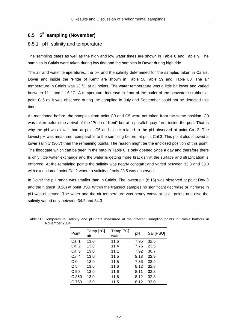
8 Results and Discussion of environmental samplings
75
8.5 5th sampling (November)
8.5.1 pH, salinity and temperature
The sampling dates as well as the high and low water times are shown in Table 8 and Table 9. The
samples in Calais were taken during low tide and the samples in Dover during high tide.
The air and water temperatures, the pH and the salinity determined for the samples taken in Calais,
Dover and inside the “Pride of Kent” are shown in Table 58,Table 59 and Table 60. The air
temperature in Calais was 13 °C at all points. The water temperature was a little bit lower and varied
between 11.1 and 11.6 °C. A temperature increase in front of the outlet of the seawater scrubber at
point C 5 as it was observed during the sampling in July and September could not be detected this
time.
As mentioned before, the samples from point C0 and C5 were not taken from the same position. C0
was taken before the arrival of the “Pride of Kent” but at a parallel quay farer inside the port. That is
why the pH was lower than at point C5 and closer related to the pH observed at point Cal 2. The
lowest pH was measured, comparable to the sampling before, at point Cal 3. This point also showed a
lower salinity (30.7) than the remaining points. The reason might be the enclosed position of this point.
The floodgate which can be seen in the map in Table 6 is only opened twice a day and therefore there
is only little water exchange and the water is getting more brackish at the surface and stratification is
enforced. At the remaining points the salinity was nearly constant and varied between 32.8 and 33.0
with exception of point Cal 2 where a salinity of only 23.5 was observed.
In Dover the pH range was smaller than in Calais. The lowest pH (8.15) was observed at point Dov 3
and the highest (8.26) at point D50. Within the transect samples no significant decrease or increase in
pH was observed. The water and the air temperature was nearly constant at all points and also the
salinity varied only between 34.2 and 34.3
Table 58: Temperature, salinity and pH data measured at the different sampling points in Calais harbour inNovember 2004
Point Temp [°C]air
Temp [°C]water pH Sal [PSU]
Cal 1 13.0 11.6 7.95 32.5Cal 2 13.0 11.4 7.76 23.5Cal 3 13.0 11.1 7.92 30.7Cal 4 13.0 11.5 8.18 32.9C 0 13.0 11.5 7.86 32.9C 5 13.0 11.6 8.12 32.8C 50 13.0 11.6 8.11 32.8C 350 13.0 11.6 8.12 32.8C 750 13.0 11.5 8.12 33.0
This document, and more, is available for download at Martin's Marine Engineering Page - www.dieselduck.net

8 Results and Discussion of environmental samplings
76
Table 59: Temperature, salinity and pH data measured at the different sampling points in Dover harbour inNovember 2004
Point Temp [°C]air
Temp [°C]water pH Sal [PSU]
D 0 13.0 11.7 8.23 34.2D 5 13.0 11.6 8.24 34.2D 50 13.0 11.6 8.26 34.3D 350 13.0 11.7 8.25 34.3D 750 13.0 11.6 8.17 34.3Dov 1 13.0 11.6 8.21 34.4Dov 2 13.0 11.6 8.18 34.4Dov 3 13.0 11.5 8.15 34.3Dov 4 13.0 11.5 8.19 34.3
Table 60: Temperature, salinity and pH data measured at the different sampling points in the seawater scrubberharbour in November 2004
Point Temp [°C]water pH Sal [PSU]
SD1 13.2 8.32 33.9SD2 27.4 6.47 34.8SCH1 14.0 8.28 34.3SCH2 26.2 6.66 35.0SCH3 35.5 3.35 35.7SCH4 34.1 2.67 35.9SCH5 35.4 3.34 35.6SCH6 36.9 3.30 35.8SCH8 24.1 3.79 35.0SC1 13.6 7.81 33.0SC2 25.5 6.33 33.5
Inside the seawater scrubber system the water temperature was highly variable. The lowest
temperatures (13.2, 14.0 and 13.6 °C) were measured in the inlet samples. In the outlet the
temperature was about 12 to 14 °C higher. The highest temperature was measured at point SCH6
(36.9 °C) directly behind the seawater scrubber. It slightly decreased at points SCH3 and SCH5 to
35.5 °C. The salinity inside the channel was slightly higher than inside the ports of Dover and Calais.
The pH values in the inlet were 8.32 in Dover, 8.28 in the Channel and 7.81 in Calais. These values
are comparable to the values measured outside the “Pride of Kent”. The lowest pH was measured at
point SCH4. An explanation might be an overflow valve from the funnel reaching the pipe shortly
before the sampling point. The pH values at points SCH6, SCH5 and SCH3 were nearly constant with
3.30, 3.34 and 3.35. The outflowing water showed a pH between 6.33 and 6.66. It can be seen that
the dilution with cooling water increased the pH and directly in front of the outlet no decrease in pH
was measured.
This document, and more, is available for download at Martin's Marine Engineering Page - www.dieselduck.net

8 Results and Discussion of environmental samplings
77
8.5.2 Metals and Sulphate
The sulphate, earth and transition metal contents are shown in Table 61. It can be seen that
chromium, manganese and molybdenum could only be determined in the settling tank and in the pipe
leading to the settling tank. The reason for this might be, as explained before, the low pH and the
concentration of particles in the cyclones and the settling tank.
Copper was measured at all points with the exception of point SCH1. An increase of the copper
content due to the seawater scrubber cannot be stated for sure especially as during the sampling in
September no copper could be determined. During the sampling in March high copper concentrations
were also detected inside the settling tank. With respect to the inlet and outlet samples, copper is even
decreasing in Calais.
The iron contents were again highest inside the settling tank. Here values up to 70 times higher than
those at the remaining seawater scrubber points were observed. In the outlet water only in Dover an
increased iron content was measured. Molybdenum, vanadium and nickel, also contents of ship steel,
were found especially in the seawater scrubber system. Tin concentrations varied in the system but
were higher in the outlet samples in comparison to the inlet samples. At point SCH4 no tin was found
and inside the settling tank no increased tin content was observed. This again shows that the
determined tin most probably originates from the sampling procedure. Potassium, lithium and
magnesium had equal contents in all samples. These earth metals are conservative due to their
reactivity and their concentration only depends on salinity.
Table 61: Sulphate, earth and transition metals determined for the samples taken in November 2004
SC1 SC2 C 5 SCH1 SCH2 SCH3 SCH4 SCH5 SCH6 SCH8 SD1 SD2 D 5Ca ppm 397 402 384 368 400 400 407 406 406 405 385 388 388Cr ppb - - - - - - 74 - - 362 - - -Cu ppb 119 48 35 32 74 40 60 100 1138 37 48 46Fe ppb - - 74 - - 750 5292 481 585 33479 62 93 79K ppm 388 392 353 352 386 382 386 378 381 379 359 355 361Li ppm 178 180 163 168 184 181 183 184 183 183 170 170 167Mg ppm 1238 1251 1186 1157 1256 1255 1272 1263 1270 1251 1198 1185 1239Mn ppb - - - - - - - - - 148 - - -Mo ppb - - - - - - - - - 13 - - 12Ni ppb - 34 - - - 68 150 59 64 583 - - -Pb ppb 31 24 - - 18 - - - - - - 34 -SO4 ppm 2699 2864 2578 2685 2805 3008 3140 3055 3061 3038 2587 2644 2669Sr ppm 8008 8054 7489 7693 8278 8087 8118 8264 8183 8203 7821 7731 7496V ppb - - - - - 197 304 201 208 2676 - 29 -Zn ppb - 229 - - 96 426 - 266 454 465 31 147 -
This document, and more, is available for download at Martin's Marine Engineering Page - www.dieselduck.net

8 Results and Discussion of environmental samplings
78
8.5.3 Nutrients
The seston and nutrient concentrations determined for the samples taken in November 2004 are
shown in Table 62. In Calais the mean seston contents were about 100 mg L-1 higher than those
observed in Dover. The highest concentrations were observed at points Cal 3 and Cal 4. The lowest
were determined for point Dov 3. Inside the seawater scrubber system a significant increase was only
measured at point SCH8. Comparing the inlet and outlet it can be seen that the concentrations in the
inlet samples are comparable to those measured inside the harbours. In Dover the outlet water
contained more suspended material than the inlet water. In Calais and in the Channel it was the
reverse case. In Calais the concentration was even the half the concentration of the inlet sample.
Table 62: Seston and nutrient concentrations determined for the samples taken in November 2004
samp.point
Seston RDP DOP TDP NO2- NO3
- NH4+ DIN Si(OH)4
[mg L-1] [µmol L-1] [µmol L-1] [µmol L-1] [µmol L-1] [µmol L -1] [µmol L -1] [µmol L -1] [µmol L-1]Cal1 148.9 0.70 4.89 5.59 0.82 14.51 10.72 26.05 22.23Cal2 122.1 12.97 2.25 10.73 3.32 44.86 27.10 75.27 124.14Cal3 181.1 1.21 0.66 1.87 2.29 26.71 14.75 43.75 32.22Cal4 184.9 0.59 2.75 3.35 0.89 14.41 9.48 24.78 20.81C0 101.6 0.86 5.81 6.67 0.76 12.26 9.79 22.81 18.16C5 93.1 0.15 1.52 1.67 1.50 17.15 50.27 68.92 22.28C50 131.5 0.51 3.35 3.85 0.96 13.43 10.55 24.95 18.18C350 126.3 0.59 2.07 2.67 0.87 13.35 10.68 24.90 18.18C700 63.7 0.57 5.09 5.66 0.72 11.67 9.64 22.03 15.55D0 25.4 0.64 6.32 6.96 1.09 16.46 1.56 19.10 6.99D5 26.9 0.68 6.17 6.85 1.14 16.47 1.56 19.16 7.14D50 70.3 0.70 3.72 4.43 1.10 16.40 1.62 19.12 5.95D350 33.1 0.73 5.24 5.97 1.28 14.67 1.28 17.23 9.47D700 23.6 0.70 5.09 5.79 1.16 14.66 2.30 18.13 24.15Dov2 34.0 0.79 5.22 6.01 1.20 13.89 1.50 16.58 11.56Dov3 15.9 0.64 4.52 5.15 1.10 12.34 1.25 14.68 7.98Dov4 51.6 0.64 4.23 4.87 1.17 14.26 2.12 17.55 29.47SD1 28.8 0.62 - - 0.82 13.79 0.37 14.98 7.01SD2 86.5 - - - 2.36 19.47 2.75 24.57 6.19SCH1 23.2 0.37 - - 1.39 11.09 0.56 13.04 5.06SCH2 16.1 0.22 - - 2.57 11.83 2.09 16.49 4.92SCH3 67.7 1.21 - - 0.03 24.45 2.76 27.24 8.94SCH4 66.9 1.21 - - 0.41 26.76 5.16 32.33 10.39SCH5 18.7 0.81 - - 0.03 18.36 0.94 19.33 7.52SCH6 18.7 0.84 - - 0.02 18.24 0.91 19.17 7.74SCH8 407.4 0.42 - - 0.70 14.37 6.32 21.38 28.92SC1 140.0 0.29 - - 0.74 10.78 5.56 17.08 15.65SC2 73.7 0.26 - - 1.45 13.18 7.93 22.56 15.81
Looking at the phosphorus compounds in the ports it can be seen that the RDP concentration was
highest at point Cal 2 (12.97) whereas at the remaining points the concentrations varied between 0.15
(C5) and 1.21 µmol L-1 (C3). At point Cal 2 also high silicate, nitrate nitrite and ammonium
concentrations were observed. As this point is situated at the service quay in an enclosed position at
the eastern end of the harbour this point is easily eutrophicated. Inside the harbour of Calais the
nitrate, silicate and ammonium concentrations were slightly increased in comparison to the samples
taken in Dover, whereas in Dover the nitrite concentrations were increased. The reason therefore
might be the architecture of the ports. Dover has one big “basin” open at two sides and no freshwater
inflow. During each ebb and flow the water is flowing through the port and enables a marked water
This document, and more, is available for download at Martin's Marine Engineering Page - www.dieselduck.net

8 Results and Discussion of environmental samplings
79
exchange. Additionally a great part of the harbour cannot be reached from the public areas. The
opposite holds for Calais. The port has many enclosed arms and areas. Water exchange is only
possible through the relatively small gate in the west of the port. Additionally the city Calais was built
around the harbour and therefore the anthropogenic influence is greater than in Dover.
Inside the seawater scrubber system the RDP concentrations were only higher at points SCH3 and
SCH4. At the remaining points the determined concentrations were within the range observed inside
the harbour. Comparing the inlet and outlet samples an increase in nitrate, nitrite and ammonium can
be seen. In contrast inside the system especially the NO2- and NH4
+ values are low and even lower
than those observed in the outlet. Only the nitrate concentrations are slightly increased inside the
seawater scrubber due to the NOx remove from the fluegas.
8.5.4 Polycyclic Aromatic Hydrocarbons
The PAH concentrations determined for the samples taken in November are shown in Table 69,,Table
70 and Table 72. From the PAH concentrations measured in the samples taken in Calais it can be
seen that the lowest total amount was determined for point Cal 2 (225 ng L -1) and the highest for
C 350 (625 ng L-1). In Dover the lowest concentration was measured at point D 0 (106 ng L-1) and the
highest at point Dov 3 (569 ng L-1). The transect samples taken in Dover and Calais indicate a specific
trend. In Dover the samples taken 50 m away from the outlet showed the highest concentration and in
Calais that one 350 m away from the outlet. Compared to the previous samplings, the highest
concentrations were observed.
Taking a look at the seawater scrubber samples the highest amount was again determined inside the
sett ling tank. Here high concentrations of phenanthrene, fluoranthene, pyrene, chrysene and
benz[a]anthracene were measured. Also high concentrations of high molecular weight PAHs were
observed, whereas two-ring compounds were not enriched. As these compounds have a high
solubility and do not adsorb to surfaces, they are not removed by the cyclones. The concentrations in
the seawater scrubber outlet are within the same range as observed during the other samplings.
This document, and more, is available for download at Martin's Marine Engineering Page - www.dieselduck.net

8 Results and Discussion of environmental samplings
80
Quality of measurement: Comparison 1st and 2nd extraction
The regressions of the filter weights and the regression of all PAH concentrations determined for the
first and the second extraction of the samples are shown in Fig. 37. It can be seen that both values are
close to one and no outlyers are obvious.
y = 0,9964xR2 = 0,966
0,00
0,01
0,02
0,03
0,04
0,00 0,01 0,02 0,03 0,04
1st extraction
2nd
extr
acti
on
y = 0,9698xR2 = 0,9967
0
2000
4000
6000
0 2000 4000 6000 8000
1st extraction
2ndex
trac
tion
Fig. 37: Regression between the first and the second extraction. Left: filter weights, right: PAH concentrations.
Origin of PAHs
To determine the relationships between the different sampling points and to determine the origin of the
PAHs a regression analysis of the compounds (Table 63) and of the sampling points (Table 64) was
performed. Additionally a principle component analysis was carr ied out (Table 66 and Fig. 39) and a
plot of the isomeric ratios Phen/Anth and Flua/Pyr (Fig. 38) and BaA/Chry (Table 65) was drawn.
Looking at Table 63 it can be seen that nearly all compounds are highly correlated. Only anthracene
and acenaphthene show moderate R² values. To obtain a better resolution and to prevent
mathematical errors a look at Table 64 is necessary. From this it can be stated that all Calais samples
with the exception of Cal 2 show the same distribution of PAHs. Also the seawater scrubber samples
(without the inlet samples) are highly correlated with each other. Additionally the points Dov 4 and D50
seem to show different PAH patterns in comparison to the remaining samples taken in Dover. No
correlation was observed between the samples taken from the seawater scrubber and those taken in
Calais, between the seawater scrubber samples and those taken in Dover, and also between most
samples taken in Dover and Calais. In summary it can be said, that the PAH composition inside the
harbours was different from that in the seawater scrubber system with one exception: point D5 which
was taken directly in front of the seawater scrubber outlet is highly correlated with the seawater
scrubber samples. A comparably high correlation was not observed in Calais or at the remaining
transect points in Dover.
This document, and more, is available for download at Martin's Marine Engineering Page - www.dieselduck.net

8 Results and Discussion of environmental samplings
81
Table 63: Regression of PAH compounds. Colours are added for a better visualisation. Yellow - highly correlated,orange and red - moderate or low correlation, dark red - no significant correlation.
AT
HY
AT
HE
FL
RE
PH
EN
AN
TH
FL
UA
PY
R
BaA
CH
RY
Bbk
F
BaP
Dah
A
Bgh
iP
IND
E
ATHY 1 0.865 0.926 0.906 0.93 0.868 0.913 0.92 0.899 0.903 0.928 0.813 0.82 0.757ATHE 1 0.724 0.696 0.831 0.684 0.718 0.78 0.729 0.781 0.761 0.601 0.615 0.557FLRE 1 0.996 0.906 0.976 0.993 0.969 0.984 0.968 0.985 0.952 0.961 0.908PHEN 1 0.874 0.967 0.986 0.974 0.989 0.965 0.989 0.962 0.956 0.894ANTH 1 0.897 0.926 0.876 0.869 0.892 0.89 0.786 0.848 0.831FLUA 1 0.984 0.939 0.968 0.967 0.949 0.964 0.991 0.968PYR 1 0.961 0.977 0.966 0.976 0.947 0.965 0.926BaA 1 0.991 0.987 0.99 0.937 0.915 0.842CHRY 1 0.988 0.989 0.97 0.955 0.893BbkF 1 0.979 0.946 0.945 0.89BaP 1 0.934 0.925 0.853DahA 1 0.973 0.929BghiP 1 0.983INDE 1
Table 64: Regression of sampling points. Colours are added for a better visualisation. Yellow - highly correlated,orange and red - moderate or low correlation, dark red - no significant correlation.
Cal1 Cal2 Cal3 Cal4 C0 C5 C50 C350 C700 D5 D50 D350 D700 Dov2 Dov3 Dov4 D0 SD1 SD2 SCH1 SCH2 SCH3 SCH4 SCH5 SCH6 SCH8 SC1 SC2Cal1 1 0.196 0.878 0.956 0.892 0.927 0.954 0.77 0.968 0.507 0.895 0.542 0.438 0.72 0.556 0.752 0.393 0.913 0.468 0.928 0.367 0.334 0.382 0.359 0.355 0.373 0.951 0.421 Cal1Cal2 1 0.306 0.246 0.261 0.232 0.239 0.272 0.264 0.466 0.223 0.531 0.616 0.513 0.315 0.201 0.689 0.251 0.243 0.144 0.245 0.239 0.23 0.241 0.239 0.24 0.285 0.252 Cal2Cal3 1 0.929 0.928 0.96 0.96 0.965 0.907 0.717 0.916 0.78 0.654 0.887 0.836 0.823 0.605 0.855 0.653 0.737 0.573 0.546 0.589 0.573 0.562 0.604 0.925 0.632 Cal3Cal4 1 0.945 0.914 0.946 0.841 0.986 0.608 0.845 0.618 0.532 0.781 0.632 0.692 0.502 0.94 0.543 0.89 0.448 0.414 0.463 0.433 0.43 0.45 0.96 0.488 Cal4C0 1 0.891 0.905 0.853 0.938 0.765 0.816 0.735 0.663 0.865 0.737 0.659 0.601 0.963 0.753 0.85 0.663 0.628 0.678 0.647 0.646 0.657 0.974 0.695 C0C5 1 0.991 0.925 0.892 0.615 0.98 0.698 0.539 0.823 0.775 0.909 0.474 0.833 0.575 0.761 0.486 0.46 0.499 0.494 0.482 0.52 0.919 0.567 C5C50 1 0.901 0.928 0.603 0.97 0.669 0.527 0.814 0.723 0.871 0.472 0.873 0.551 0.802 0.46 0.431 0.472 0.462 0.451 0.484 0.944 0.532 C50C350 1 0.792 0.714 0.876 0.78 0.628 0.843 0.909 0.835 0.572 0.734 0.656 0.594 0.592 0.575 0.608 0.602 0.588 0.644 0.818 0.661 C350C700 1 0.589 0.831 0.607 0.533 0.776 0.589 0.667 0.507 0.951 0.528 0.934 0.429 0.393 0.446 0.412 0.411 0.426 0.969 0.464 C700D5 1 0.548 0.903 0.924 0.893 0.807 0.454 0.853 0.691 0.904 0.434 0.896 0.88 0.887 0.884 0.883 0.888 0.698 0.896 D5D50 1 0.662 0.49 0.784 0.739 0.956 0.42 0.767 0.513 0.701 0.43 0.405 0.439 0.444 0.429 0.468 0.872 0.52 D50D350 1 0.943 0.943 0.897 0.618 0.896 0.793 0.783 0.427 0.768 0.755 0.756 0.776 0.766 0.79 0.707 0.813 D350D700 1 0.89 0.76 0.416 0.963 0.591 0.78 0.374 0.782 0.768 0.765 0.773 0.771 0.774 0.627 0.783 D700Dov2 1 0.861 0.695 0.82 0.801 0.793 0.601 0.742 0.72 0.74 0.742 0.735 0.753 0.859 0.789 Dov2Dov3 1 0.741 0.672 0.58 0.78 0.396 0.757 0.755 0.763 0.782 0.765 0.819 0.674 0.826 Dov3Dov4 1 0.348 0.577 0.419 0.519 0.354 0.339 0.36 0.381 0.361 0.41 0.7152 0.458 Dov4D0 1 0.538 0.65 0.347 0.652 0.636 0.636 0.637 0.636 0.641 0.572 0.645 D0SD1 1 0.66 0.908 0.563 0.522 0.575 0.537 0.54 0.539 0.975 0.583 SD1SD2 1 0.429 0.988 0.978 0.991 0.982 0.984 0.977 0.655 0.982 SD2SCH1 1 0.327 0.291 0.345 0.307 0.31 0.31 0.892 0.35 SCH1SCH2 1 0.998 0.997 0.996 0.998 0.99 0.559 0.985 SCH2SCH3 1 0.995 0.997 0.999 0.991 0.522 0.983 SCH3SCH4 1 0.993 0.995 0.99 0.57 0.981 SCH4SCH5 1 0.999 0.996 0.546 0.993 SCH5SCH6 1 0.993 0.543 0.989 SCH6SCH8 1 0.554 0.991 SCH8SC1 1 0.603 SC1SC2 1 SC2
Table 65: Isomeric ratios of benz[a]anthracene and chrysene
sampl.point Cal 1 Cal 2 Cal 3 Cal 4 C0 C5 C50 C350 C700
BaA/CHRY 0.9 0.8 0.7 1.0 0.9 1.3 0.8 0.8 0.9
sampl.point Dov 2 Dov 3 Dov 4 D0 D5 D50 D350 D700
BaA/CHRY 0.8 0.8 0.8 0.8 0.8 0.7 0.9 0.9
sampl.point SD1 SD2 SCH1 SCH2 SC1 SC2 SCH3 SCH4 SCH5 SCH6 SCH8
BaA/CHRY 1.7 1.9 1.0 0.5 0.8 0.6 0.5 0.5 0.5 0.6 0.5
This document, and more, is available for download at Martin's Marine Engineering Page - www.dieselduck.net

8 Results and Discussion of environmental samplings
82
0
10
20
30
40
50
60
70
80
90
100
0,0 0,5 1,0 1,5 2,0
phenanthrene / anthracene
flu
ora
nth
ene
/p
yre
ne
DoverCalaisSWSoutlet
petrogenic
pyrolytic
Fig. 38: Plot of isomeric phenanthrene/anthracene ratios against fluoranthene/pyrene ratios for all samples
Taking a look at the BaA/Chry ratios (Table 65) it can be seen that all values, with exception of SD1,
SD2 and D5 are <1 and therefore indicate a pyrolytic origin. In Fig. 38 where the
phenanthrene/anthracene and fluoranthene/pyrene ratios are plotted, only the samples taken from the
seawater scrubber outlet and the seawater scrubber system itself show petrogenic character. The
remaining samples, especially those taken in Calais, seem to originate from combustion processes.
As the samples were taken in fall when the heating season starts, these PAHs are most probably
PAHs produced by burning wood, heating oil and gas.
The principal component plot shows the similar separation of the samples as the regression chart
already did. Sample Cal 2 is an outlyer, showing only low concentrations. Dov 2 is correlated with
C700, C350 and C005 and these samples are also located in one group in the PCA plot. Additionally
D50, SD1 and Cal1 are within this group. All these samples show negative values for eigenvector 2
which is positive for low molecular weight and negative for high molecular weight PAHs. The samples
show a similar distribution but as eigenvector 2 is only responsible for 20 % of the total variance it is
not significant. According to their distribution along eigenvector 2 the samples can partially be divided
into PAHs originating from petrogenic (negative) or pyrolytic (positive) pollution sources. Thereafter
D50 has the most petrogenic and Cal 4 and C 700 the most pyrolytic character. This can easily be
explained by the positions of these points. Cal 4 and C 700 are the most eastern points in the port
Calais and are situated at the entrance. These points are therefore influenced by North Sea water
reaching the harbour. There the main pollution source is the atmosphere, which carries especially
PAHs from pyrolytic processes. Inside the port the influence of the shipping activities is greater and
this direct pollution is of petrogenic origin.
This document, and more, is available for download at Martin's Marine Engineering Page - www.dieselduck.net
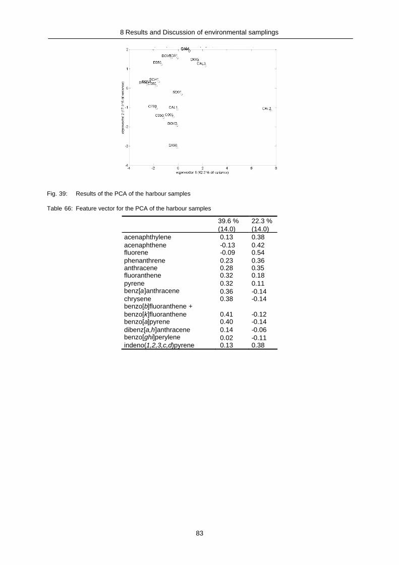
8 Results and Discussion of environmental samplings
83
Fig. 39: Results of the PCA of the harbour samples
Table 66: Feature vector for the PCA of the harbour samples
39.6 %(14.0)
22.3 %(14.0)
acenaphthylene 0.13 0.38acenaphthene -0.13 0.42fluorene -0.09 0.54phenanthrene 0.23 0.36anthracene 0.28 0.35fluoranthene 0.32 0.18pyrene 0.32 0.11benz[a]anthracene 0.36 -0.14chrysene 0.38 -0.14benzo[b]fluoranthene +benzo[k]fluoranthene 0.41 -0.12benzo[a]pyrene 0.40 -0.14dibenz[a,h]anthracene 0.14 -0.06benzo[ghi]perylene 0.02 -0.11indeno(1,2,3,c,d)pyrene 0.13 0.38
This document, and more, is available for download at Martin's Marine Engineering Page - www.dieselduck.net

9 Results and discussion of the toxicity and accumulation tests
84
8.6 Annual circle
8.6.1 pH, salinity and temperature
In this chapter the temperature, salinity and pH values determined during all samplings are shown.
Inside the “Pride of Kent“ not at all points samples were taken during every sampling. In February the
seawater scrubber was not active and therefore only samples from the inlet and outlet were taken.
During the sampling in July sampling points 4, 7 and 8 were closed and in September and November
the settling tank was not full enough to take a sample from point 7. For samples taken inside the
harbour of Calais (Fig. 40, ,Fig. 41) values for all samplings are available. It can be seen that the
highest temperatures were measured in late summer during the sampling in September. Here the
water temperature was about 22 °C and thus about 15 °C higher than during the sampling in February.
The salinity at point Cal 4 was relative stable and higher than at point Cal 1 to Cal 3. This point is
situated close to the harbour entrance and is therefore influenced by the North Sea where the salinity
is relatively stable. The farer inside the sampling point was located in the harbour the higher the
variability was. At point Cal 2 at the eastern end of a long sidearm the salinity varied within a wide
range (18.3 to 34.0). As the pH in brackish and fresh water is lower than in salt water, the pH was also
very variable at this point (7.76 - 8.50).
Cal 1: Quai en eau profonde
7,97 7,957,958,427,69
32,5
7,4 8,5
17,0
11,6
27,0
34,129,0
31,2
22,1
0
2
4
6
8
10
11.02
.04
24.03
.04
14.07
.04
08.09
.04
16.11
.04
sampling date
pH
0510152025303540
salin
ity[p
SU
]te
mpe
ratu
re[°
C]
pHSalTemp
Cal 2: Quai de service
7,81 8,07 7,768,5 7,97
23,5
7,3 8,5
17,1
11,4
31,7 31,034,0
18,322,1
0
2
4
6
8
10
11.02
.04
24.03
.04
14.07
.04
08.09
.04
16.11
.04
sampling date
pH
0510152025303540
sali
nity
[pS
U]
tem
pera
ture
[°C
]
pHSalTemp
Fig. 40: Salinity, temperature, and pH measured at points Cal 1 and Cal 2
Cal 3: Quai de la Loire
8,289,35 7,89
8,04 7,92
7,3 7,7
16,5
11,1
27,5 29,0 31,929,6 30,7
21,5
0
2
4
6
8
10
11.02
.04
24.03
.04
14.07
.04
08.09
.04
16.11
.04
sampling date
pH
05101520253035
sali
nity
[pSU
]te
mpe
ratu
re[°
C]
pHSalTemp
Cal 4: Jetee ouest
8,22 8,188,02 8,048,63
32,9
7,4 8,5
16,9
11,5
31,033,732,031,5
21,9
0
2
4
6
8
10
11.02
.04
24.03
.04
14.07
.04
08.09
.04
16.11
.04
sampling date
pH
0510152025303540
sali
nity
[pSU
]te
mpe
ratu
re[°
C]
pHSalTemp
Fig. 41: Salinity, temperature, and pH measured at points Cal 3 and Cal 4
Samples from the transect points in Calais were only taken in July, September and November. The
annual course is shown in Fig. 43 and Fig. 44. As these points were situated inside the harbour the
This document, and more, is available for download at Martin's Marine Engineering Page - www.dieselduck.net
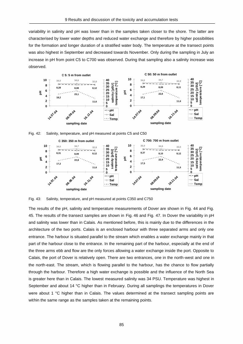
9 Results and discussion of the toxicity and accumulation tests
85
variability in salinity and pH was lower than in the samples taken closer to the shore. The latter are
characterised by lower water depths and reduced water exchange and therefore by higher possibilities
for the formation and longer duration of a stratified water body. The temperature at the transect points
was also highest in September and decreased towards November. Only during the sampling in July an
increase in pH from point C5 to C700 was observed. During that sampling also a salinity increase was
observed.
C 5: 5 m from outlet
8,28 8,128,08
18,223,1
11,6
34,0 32,834,6
0
2
4
6
8
10
14.07.0
4
08.09.0
4
16.11.0
4
sampling date
pH
0510152025303540
salin
ity
[pS
U]
tem
per
atu
re[°
C]
pHSalTemp
C 50: 50 m from outlet
8,29 8,118,09
17,1
22,8
11,6
34,0 32,834,7
0
2
4
6
8
10
14.07.0
4
08.09.0
4
16.11.0
4
sampling datep
H
0510152025303540
sali
nity
[pS
U]
tem
pera
ture
[°C
]
pHSalTemp
Fig. 42: Salinity, temperature, and pH measured at points C5 and C50
C 350: 350 m from outlet
8,31 8,128,09
17,2
22,8
11,6
34,0 32,834,7
0
2
4
6
8
10
14.07
.04
08.09
.04
16.11
.04
sampling date
pH
0510152025303540
sal
inity
[pS
U]
tem
per
atur
e[°
C]
pHSalTemp
C 700: 700 m from outlet
8,37 8,128,10
17,5
22,9
11,5
35,0 33,034,6
0
2
4
6
8
10
14.07
.04
08.09
.04
16.11
.04
sampling date
pH
0510152025303540
sali
nity
[pS
U]
tem
per
atu
re[°
C]
pHSalTemp
Fig. 43: Salinity, temperature, and pH measured at points C350 and C750
The results of the pH, salinity and temperature measurements of Dover are shown in Fig. 44 and Fig.
45. The results of the transect samples are shown in Fig. 46 and Fig. 47. In Dover the variability in pH
and salinity was lower than in Calais. As mentioned before, this is mainly due to the differences in the
architecture of the two ports. Calais is an enclosed harbour with three separated arms and only one
entrance. The harbour is situated parallel to the stream which enables a water exchange mainly in that
part of the harbour close to the entrance. In the remaining part of the harbour, especially at the end of
the three arms ebb and flow are the only forces allowing a water exchange inside the port. Opposite to
Calais, the port of Dover is relatively open. There are two entrances, one in the north-west and one in
the north-east. The stream, which is flowing parallel to the harbour, has the chance to flow partially
through the harbour. Therefore a high water exchange is possible and the influence of the North Sea
is greater here than in Calais. The lowest measured salinity was 34 PSU. Temperature was highest in
September and about 14 °C higher than in February. During all samplings the temperatures in Dover
were about 1 °C higher than in Calais. The values determined at the transect sampling points are
within the same range as the samples taken at the remaining points.
This document, and more, is available for download at Martin's Marine Engineering Page - www.dieselduck.net

9 Results and discussion of the toxicity and accumulation tests
86
Dov 1: eastern entrance
8,10 8,07 8,218,35
8,4
15,9
22,2
11,6
34,0 34,435,034,0
0
2
4
6
8
10
11.02
.04
14.07
.04
08.09
.04
16.11
.04
sampling date
pH
0510152025303540
salin
ity
[pS
U]
tem
per
atu
re[°
C]
pHSalTemp
Dov 2: east entrance
8,35 8,188,08
15,9
22,2
11,6
34,0 34,435,1
0
2
4
6
8
10
14.07
.04
08.09
.04
16.11
.04
sampling date
pH
0510152025303540
salin
ity
[pS
U]
tem
pera
ture
[°C
]
pHSalTemp
Fig. 44: Salinity, temperature, and pH measured at points Dov 1 and Dov 2
Dov 3: middle port
8,35 8,158,08
15,9
21,9
11,5
34,0 34,335,1
0
2
4
6
8
10
14.0
7.04
08.09.0
4
16.1
1.04
sampling date
pH
0510152025303540
salin
ity
[pS
U]
tem
per
atu
re[°
C]
pHSalTemp
Dov 4: western port
8,37 8,198,08
15,9
22,2
11,5
34,0 34,335,2
0
2
4
6
8
10
14.07
.04
08.09
.04
16.11
.04
sampling date
pH
0510152025303540
sal
inity
[pS
U]
tem
per
atur
e[°
C]
pHSalTemp
Fig. 45: Salinity, temperature, and pH measured at points Dov 3 and Dov 4
D 5: 5 m from outlet
7,95 8,07 8,248,35
8,8
15,9
22,8
11,6
34,4 34,235,134,0
0
2
4
6
8
10
24.03
.04
14.07
.04
08.09
.04
16.11
.04
sampling date
pH
0510152025303540
sal
inity
[pS
U]
tem
per
atur
e[°
C]
pHSalTemp
D 50: 50 m from outlet
8,00 8,04 8,268,35
8,8
15,9
22,3
11,6
34,4 34,335,234,0
0
2
4
6
8
10
24.03
.04
14.07
.04
08.09
.04
16.11
.04
sampling date
pH
0510152025303540
sal
inity
[pS
U]
tem
per
atur
e[°
C]
pHSalTemp
Fig. 46: Salinity, temperature, and pH measured at points D5 and D50
D 350: 350 m from outlet
8,35 8,258,05
15,9
22,1
11,7
34,0 34,335,0
0
2
4
6
8
10
14.07
.04
08.09
.04
16.11
.04
sampling date
pH
0510152025303540
sali
nity
[pSU
]te
mpe
ratu
re[°
C]
pHSalTemp
D 700: west entrance
8,10 8,04 8,178,38
8,5
15,9
22,1
11,6
34,1 34,335,034,0
0
2
4
6
8
10
11.02
.04
14.07
.04
08.09
.04
16.11
.04
sampling date
pH
0510152025303540
sal
inity
[pS
U]
tem
per
atur
e[°
C]
pHSalTemp
Fig. 47: Salinity, temperature, and pH measured at points D350 and D700
This document, and more, is available for download at Martin's Marine Engineering Page - www.dieselduck.net

9 Results and discussion of the toxicity and accumulation tests
87
Table 67: Differences between the inlet and outlet samples taken from the seawater scrubber system in Calais,Dover and the Channel. Left: pH difference. Right: temperature difference
pH March July Sept. Nov. Temp [°C] March July Sept. Nov.Dover 0.43 1.51 1.79 1.85 Dover 4.1 2.9 13.6 14.2Channel 1.16 1.45 1.68 1.62 Channel 1.9 2.8 14.1 12.2Calais 0.66 1.34 1.73 1.48 Calais 3.3 2.7 16.9 11.9
The annual course of the salinity, pH and temperature of the inlet and outlet samples is shown in Fig.
48 (Dover), Fig. 49 (Calais) and Fig. 50 (Channel). The pH, the temperature and the salinity of the inlet
samples taken in Dover and Calais are within the same range as the samples taken in the ports. Only
the sample taken in Calais in September shows a relatively low pH, but this is comparable to the
sample taken at point Cal 2 (Table 49). As the samples from point SC1 were not taken at the same
time and not directly at the pier but during entering the harbour, small variations are possible.
Therefore it can be said, that the values are comparable and an influence of the outlet water onto the
inlet water can be mainly excluded. Looking at the outlet samples, also an annual influence onto the
temperature is obvious. The temperature of the outlet is strongly dependent of the inlet temperature.
but as the difference between the inlet and outlet temperatures was greater in September and
November than during the samplings in February, March and July (Table 67) the main influence is by
the seawater scrubber.
The lowest pH in the outlet was measured in September as well. The reason therefore might also be
differences in the efficiency of the Ecosilencer. Another reason could be the relatively high
temperature of the effluent, because the pH is also temperature dependent. To determine this
dependency a small test was performed. 500 mL seawater (Jade Bay, Table 1) were heated and
cooled down again and the pH was measured continuously. It can be seen that the higher the
temperature was, the lower the pH was. The different ascent between heating and cooling is a
physical effect called hysteresis. If calcium carbonate is dissolved in water the following reaction
occurs:
CaCO3 + H2O + CO2 Ca(HCO3)2
An increase in the temperature shifts the equilibrium towards the left side. Therefore more CO2 is
introduced and carbonic acid is built according to:
CO2 + H2O H2CO3 H+ + HCO3- 2 H+ + CO3
2-
This reduces the pH. When the water is cooled down again the CO2 solubility increases and carbonic
acid concentration is reduced, resulting in a pH increase. As during the heating process the CO2 has
to leave the water this step takes more time in comparison to the increase in solubility.
This document, and more, is available for download at Martin's Marine Engineering Page - www.dieselduck.net
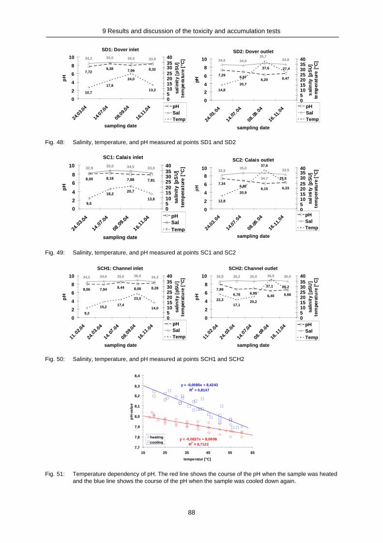
9 Results and discussion of the toxicity and accumulation tests
88
SD1: Dover inlet
7,72 7,99 8,328,38
10,7
17,8
24,0
13,2
34,2 33,934,435,0
0
2
4
6
8
10
24.03.0
4
14.0
7.04
08.09.0
4
16.11.0
4
sampling date
pH
0510152025303540
sali
nity
[pS
U]
tem
pera
ture
[°C
]
pHSalTemp
SD2: Dover outlet
7,296,20
6,87 6,47
14,8
20,7
34,035,7
34,834,6
37,6 27,4
0
2
4
6
8
10
24.03
.04
14.07
.04
08.09
.04
16.11
.04
sampling date
pH
0510152025303540
sal
inity
[pS
U]
tem
per
atur
e[°
C]
pHSalTemp
Fig. 48: Salinity, temperature, and pH measured at points SD1 and SD2
SC1: Calais inlet
8,00 7,888,16 7,81
18,213,6
35,0 34,5 33,032,9
9,5
20,7
0
2
4
6
8
10
24.0
3.04
14.07.0
4
08.09.0
4
1 6.11
.04
sampling date
pH
0510152025303540
salin
ity
[pS
U]
tem
per
atu
re[°
C]
pHSalTemp
SC2: Calais outlet
7,346,15 6,336,82
20,9
32,9 33,5
34,7
35,037,6
12,8
25,5
0
2
4
6
8
10
24.03
.04
14.07
.04
08.09
.04
16.11
.04
sampling date
pH
0510152025303540
sali
nity
[pS
U]
tem
per
atu
re[°
C]
pHSalTemp
Fig. 49: Salinity, temperature, and pH measured at points SC1 and SC2
SCH1: Channel inlet
8,06 8,44 8,287,94 8,08
34,3
9,2
15,2
23,0
14,0
34,9 35,0 36,034,3
17,4
0
2
4
6
8
10
11.0
2.04
24.03.0
4
14.07.0
4
08.09.0
4
16.11.0
4
sampling date
pH
0510152025303540
salin
ity
[pS
U]
tem
pera
ture
[°C
]
pHSalTemp
SCH2: Channel outlet
7,996,99 6,666,406,78
35,0
22,317,1
34,9 36,035,035,2
26,237,1
20,2
0
2
4
6
8
10
11.02.0
4
24.03.0
4
14.07.0
4
08.09.0
4
16.1
1.04
sampling date
pH
0510152025303540
salin
ity
[pS
U]
tem
pera
ture
[°C
]
pHSalTemp
Fig. 50: Salinity, temperature, and pH measured at points SCH1 and SCH2
y = -0,0037x + 8,0609R2 = 0,7122
y = -0,0085x + 8,4243R2 = 0,8147
7,7
7,8
7,9
8,0
8,1
8,2
8,3
8,4
15 25 35 45 55 65
temperatur [°C]
pH
-va
lue
heatingcooling
Fig. 51: Temperature dependency of pH. The red line shows the course of the pH when the sample was heatedand the blue line shows the course of the pH when the sample was cooled down again.
This document, and more, is available for download at Martin's Marine Engineering Page - www.dieselduck.net

9 Results and discussion of the toxicity and accumulation tests
89
The comparison of all samples taken at the points SCH3, SCH5 and SCH6 are shown in Fig. 52 and
Fig. 53. The salinity in these samples was always relatively high in comparison to the samples taken
inside the harbours and was highest in September. In September also the highest temperature was
measured. The lowest pH was determined in the samples taken during the second sampling. As the
system was not working completely in March the reason could be a slower flow speed of the water
through the Ecosilencer and therefore a higher saturation with sulphuric and nitric acid.
SCH3: Channel outlet US-filter
2,73 3,143,14 3,35
36,7 35,5
34,5 36,8 35,7
35,5
45,3
27,6
0
2
4
6
8
10
24.03
.04
14.07
.04
08.09
.04
16.11
.04
sampling date
pH
0
10
20
30
40
50
sal
init
y[p
SU
]te
mp
erat
ure
[°C
]
pHSalTemp
SCH5: Channel inlet US-filter
2,82 3,053,13 3,34
36,0 35,4
35,0 36,8 35,6
35,2
27,9
46,2
0
2
4
6
8
10
24.03
.04
14.07
.04
08.09
.04
16.11
.04
sampling date
pH
0
10
20
30
40
50
sali
nity
[pS
U]
tem
pera
ture
[°C
]
pHSalTemp
Fig. 52: Salinity, temperature, and pH measured at points SCH3 and SCH5
SCH6: Channel outlet Ecosilencer
2,78 3,13 3,303,09
37,0 36,935,2
35,836,435,0
45,1
28,0
0
2
4
6
8
10
24.03.0
4
14.07.0
4
08.09.0
4
16.11.0
4
sampling date
pH
0
10
20
30
40
50sa
linit
y[p
SU
]te
mp
erat
ure
[°C
]
pHSalTemp
Fig. 53: Salinity, temperature, and pH measured at point SCH6
A plot of all pH values observed during all sampling is shown in Fig. 54 and Fig. 55. The error bars
show the maximum allowed pH change caused by effluents outside the initial mixing zone (US-EPA
1986). In both graphs it can be seen that the natural pH range is greater than the pH change within the
sample suite taken at the transect points. The same can be seen in Fig. 56. During no sampling a pH
decrease from the first transect point towards the harbour entrance was observed.
From Fig. 58 where all the measured temperatures of all sampling points (without seawater scrubber
system) are shown, it can be seen that the highest temperature differences were observed inside the
ports in March. The temperatures measured at the transect points in July were partially higher than
those measured at the remaining points inside the harbour. In detail this is shown in Fig. 57. It can be
seen that during the sampling in July and September the temperatures were higher at the first transect
point in comparison to the remaining points. During the sampling in September the difference between
the inlet and the outlet temperature was also very high (Table 67). In July the difference was over
This document, and more, is available for download at Martin's Marine Engineering Page - www.dieselduck.net
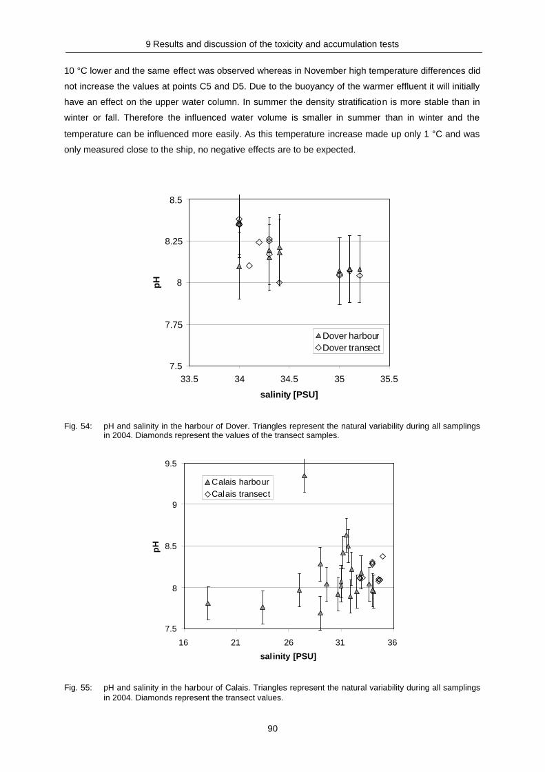
9 Results and discussion of the toxicity and accumulation tests
90
10 °C lower and the same effect was observed whereas in November high temperature differences did
not increase the values at points C5 and D5. Due to the buoyancy of the warmer effluent it will initially
have an effect on the upper water column. In summer the density stratification is more stable than in
winter or fall. Therefore the influenced water volume is smaller in summer than in winter and the
temperature can be influenced more easily. As this temperature increase made up only 1 °C and was
only measured close to the ship, no negative effects are to be expected.
7.5
7.75
8
8.25
8.5
33.5 34 34.5 35 35.5
salinity [PSU]
pH
Dover harbourDover transect
Fig. 54: pH and salinity in the harbour of Dover. Triangles represent the natural variability during all samplingsin 2004. Diamonds represent the values of the transect samples.
7.5
8
8.5
9
9.5
16 21 26 31 36
salinity [PSU]
pH
Calais harbourCalais transect
Fig. 55: pH and salinity in the harbour of Calais. Triangles represent the natural variability during all samplingsin 2004. Diamonds represent the transect values.
This document, and more, is available for download at Martin's Marine Engineering Page - www.dieselduck.net

9 Results and discussion of the toxicity and accumulation tests
91
6,8
7
7,2
7,4
7,6
7,8
8
8,2
8,4
8,6
8,8
0 200 400 600
distance from oulet [m]
pH
Calais 14.07.2004Calais 08.09.2004Calais 16.11.2004Dover 14.07.2004
Dover 08.09.2004Dover 16.11.2004
Fig. 56: pH impact of SWS effluents on the receiving harbour water in Dover and Calais at three sampling (July,Sept. and Nov.)
0
5
10
15
20
25
0 200 400 600
distance from outlet [m]
tem
pe
ratu
re[°
C]
Calais 14.07.2004Calais 08.09.2004Calais 16.11.2004Dover 14.07.2004Dover 08.09.2004Dover 16.11.2004
Fig. 57: Temperature [°C] impact of SWS effluents on the receiving harbour water in Dover and Calais at threesampling (July, Sept. and Nov.)
0
5
10
15
20
25
Jan. 0
4
Mrz . 0
4
Apr.04
Jun.04
Aug. 04
Sep. 04
Nov. 04
Dez. 04
sampling date
tem
per
atu
re[°
C]
harbourtransect
Fig. 58: Temperatures [°C] of harbour and transect samples.
This document, and more, is available for download at Martin's Marine Engineering Page - www.dieselduck.net

9 Results and discussion of the toxicity and accumulation tests
92
8.6.2 Nitrate and sulphate
Nitrate
In Fig. 59 the nitrate concentrations determined in the ports and for the inlet and outlet samples are
shown. It can be seen that in summer the concentrations were lower than in winter and fall. Because
nitrogen is an essential compound for marine primary production it is depleted in summer when the
phytoplankton production is high and nitrogen availability is a limiting factor. In winter when the
plankton production is generally close to zero the nitrogen is remineralised and its concentration
increases. Additionally in Fig. 59 the nitrate concentrations of the inlet and the outlet water are shown.
It can be seen that in Calais the outlet concentration was within the natural range whereas in Dover it
was slightly higher. The transect points did not show a nitrate concentration increase during any
sampling and were all within the natural range.
0
10
20
30
40
50
60
70
80
Feb. Mar. Jul. Sep. Nov.
sampling date
NO
3-c
on
ce
ntr
atio
n[µ
mo
ll-
1]
Cal1Cal2Cal3Cal4C5C50C350C700SC1SC2
0
10
20
30
40
50
60
70
80
Feb. Mar. Jul. Sep. Nov.
sampling date
NO
3-
co
nce
ntr
ati
on
[µm
oll
-1]
Dov2Dov4D5D50D350D700SD1SD2
Fig. 59: Nitrate concentrations [µmol l-1] observed during all samplings. Left: Port of Calais. Right: Port of Dover
The sulphate concentrations determined in the inlet and outlet of the seawater scrubber samples are
shown in Table 68. Calculating the sulphate increase between the inlet and the outlet it can be seen
that the greatest difference was observed during the sampling in November in Dover. This increase of
165 pm corresponds to a concentration change of 6.1 %. This value lies within the accuracy of the
measurement and within the natural variability.
Table 68: Comparison of sulphate inlet and outlet concentrations [ppm]
Feb. Mar. Sep. Nov.SD1 n.d. 2949 n.d. 2699SD2 n.d. 2962 2710 2864SCH1 2842 2990 2590 2685SCH2 2874 3052 2600 2805SC1 n.d. 2920 n.d. 2587SC2 n.d. 2938 2870 2644
This document, and more, is available for download at Martin's Marine Engineering Page - www.dieselduck.net
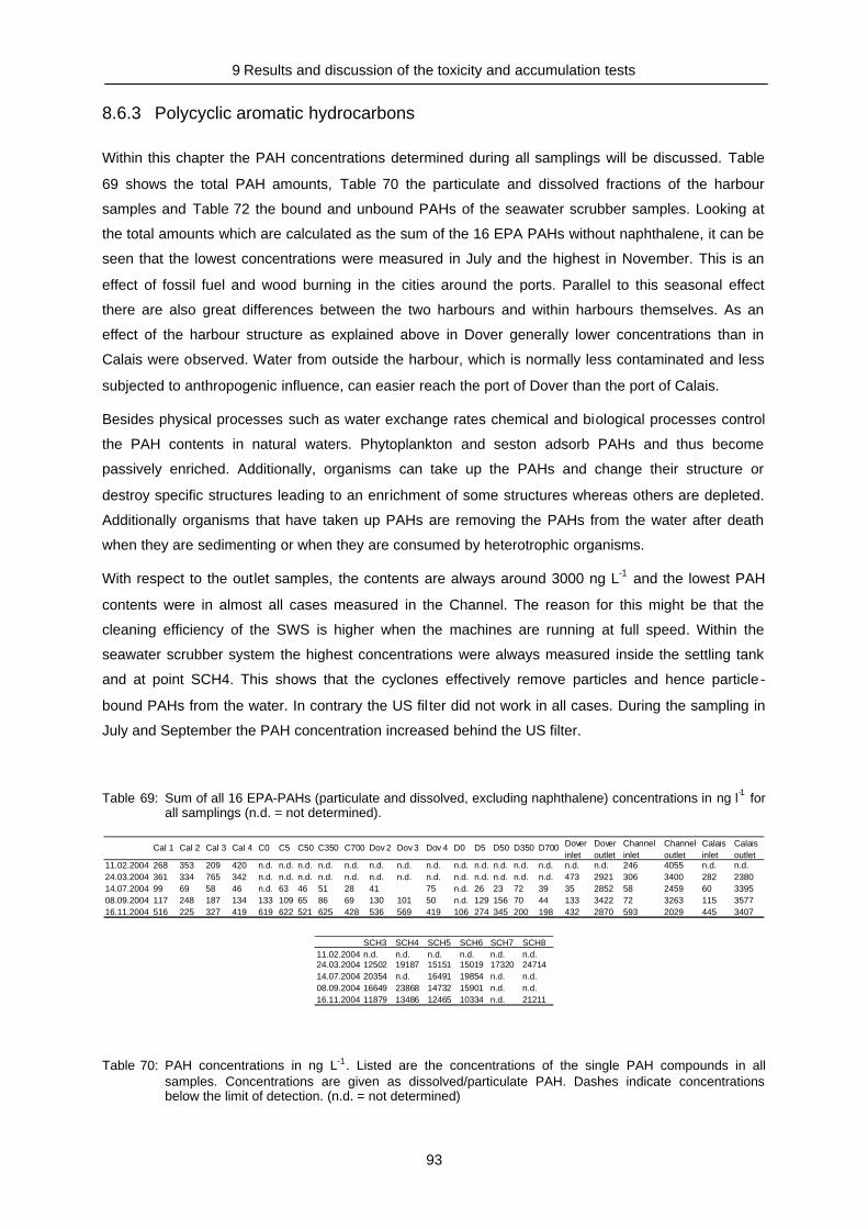
9 Results and discussion of the toxicity and accumulation tests
93
8.6.3 Polycyclic aromatic hydrocarbons
Within this chapter the PAH concentrations determined during all samplings will be discussed. Table
69 shows the total PAH amounts, Table 70 the particulate and dissolved fractions of the harbour
samples and Table 72 the bound and unbound PAHs of the seawater scrubber samples. Looking at
the total amounts which are calculated as the sum of the 16 EPA PAHs without naphthalene, it can be
seen that the lowest concentrations were measured in July and the highest in November. This is an
effect of fossil fuel and wood burning in the cities around the ports. Parallel to this seasonal effect
there are also great differences between the two harbours and within harbours themselves. As an
effect of the harbour structure as explained above in Dover generally lower concentrations than in
Calais were observed. Water from outside the harbour, which is normally less contaminated and less
subjected to anthropogenic influence, can easier reach the port of Dover than the port of Calais.
Besides physical processes such as water exchange rates chemical and biological processes control
the PAH contents in natural waters. Phytoplankton and seston adsorb PAHs and thus become
passively enriched. Additionally, organisms can take up the PAHs and change their structure or
destroy specific structures leading to an enrichment of some structures whereas others are depleted.
Additionally organisms that have taken up PAHs are removing the PAHs from the water after death
when they are sedimenting or when they are consumed by heterotrophic organisms.
With respect to the outlet samples, the contents are always around 3000 ng L-1 and the lowest PAH
contents were in almost all cases measured in the Channel. The reason for this might be that the
cleaning efficiency of the SWS is higher when the machines are running at full speed. Within the
seawater scrubber system the highest concentrations were always measured inside the settling tank
and at point SCH4. This shows that the cyclones effectively remove particles and hence particle-
bound PAHs from the water. In contrary the US fil ter did not work in all cases. During the sampling in
July and September the PAH concentration increased behind the US filter.
Table 69: Sum of all 16 EPA-PAHs (particulate and dissolved, excluding naphthalene) concentrations in ng l-1 forall samplings (n.d. = not determined).
Cal 1 Cal 2 Cal 3 Cal 4 C0 C5 C50 C350 C700 Dov 2 Dov 3 Dov 4 D0 D5 D50 D350 D700 Doverinlet
Doveroutlet
Channelinlet
Channeloutlet
Calaisinlet
Calaisoutlet
11.02.2004 268 353 209 420 n.d. n.d. n.d. n.d. n.d. n.d. n.d. n.d. n.d. n.d. n.d. n.d. n.d. n.d. n.d. 246 4055 n.d. n.d.24.03.2004 361 334 765 342 n.d. n.d. n.d. n.d. n.d. n.d. n.d. n.d. n.d. n.d. n.d. n.d. n.d. 473 2921 306 3400 282 238014.07.2004 99 69 58 46 n.d. 63 46 51 28 41 75 n.d. 26 23 72 39 35 2852 58 2459 60 339508.09.2004 117 248 187 134 133 109 65 86 69 130 101 50 n.d. 129 156 70 44 133 3422 72 3263 115 357716.11.2004 516 225 327 419 619 622 521 625 428 536 569 419 106 274 345 200 198 432 2870 593 2029 445 3407
SCH3 SCH4 SCH5 SCH6 SCH7 SCH811.02.2004 n.d. n.d. n.d. n.d. n.d. n.d.24.03.2004 12502 19187 15151 15019 17320 2471414.07.2004 20354 n.d. 16491 19854 n.d. n.d.08.09.2004 16649 23868 14732 15901 n.d. n.d.16.11.2004 11879 13486 12465 10334 n.d. 21211
Table 70: PAH concentrations in ng L-1. Listed are the concentrations of the single PAH compounds in allsamples. Concentrations are given as dissolved/particulate PAH. Dashes indicate concentrationsbelow the limit of detection. (n.d. = not determined)
This document, and more, is available for download at Martin's Marine Engineering Page - www.dieselduck.net

9 Results and discussion of the toxicity and accumulation tests
94
compound Date Cal 1 Cal 2 Cal 3 Cal 4 Dov 2 Dov 3 Dov 4 C0 C5 C50 C350 C700 D0 D5 D50 D350 D700 SD1 SD2 SCH1 SCH2 SC1 SC2ATHY 11.02.04 1/- 4/- 2/- 1/- n.d. n.d. n.d. n.d. n.d. n.d. n.d. n.d. n.d. n.d. n.d. n.d. n.d. n.d. n.d. 1/- -/25 n.d. n.d.
24.03.04 2/- 4/- 23/2 8/- n.d. n.d. n.d. n.d. n.d. n.d. n.d. n.d. n.d. n.d. n.d. n.d. n.d. 1/- 7/- 1/- 9/1 2/- 10/-14.07.04 8/- 3/- 9/- 8/- 4/- n.d. 2/- -/- -/- 1/- -/- -/- -/- -/- 2/- -/- 6/- 6/- -/- -/- 4/-08.09.04 1/- 1/- -/- 1/- -/- -/- -/- 4/- -/- -/- -/- -/- -/- -/- -/- -/- -/- 2/- -/- 7/- -/- 3/-16.11.04 9/- 8/- 11/- 12/- 28/- 12/- 9/- 9/- 14/- 14/- 12/- 13/- 7/- 8/- 8/- 11/- 10/- 13/- 14/- 8/- 13/- 13/- 23/1
ATHE 11.02.04 7/- 16/- 5/- 6/- n.d. n.d. n.d. n.d. n.d. n.d. n.d. n.d. n.d. n.d. n.d. n.d. n.d. n.d. n.d. 5/- -/120 n.d. n.d.24.03.04 7/- 8/- 15/1 7/- n.d. n.d. n.d. n.d. n.d. n.d. n.d. n.d. n.d. n.d. n.d. n.d. n.d. 6/- 30/1 5/- 43/3 8/- 32/114.07.04 -/- 8/- 4/- 4/- 2/- n.d. 5/- n.d. 3/- 2/- 4/- 3/- 3/- 1/- 2/- 2/- 1/- 28/- 1/- 1/- 2/- 2/-08.09.04 5/- 6/- 7/- 3/- 3/- 3/- 3/- 4/- 3/- 2/- 3/- 3/- 3/- 1/- 4/- 2/- 4/- 23/1 3/- 34/1 5/- 45/216.11.04 17/- 72/1 14/- 16/- 45/- 20/- 18/- 19/- 20/- 19/- 21/- 20/- 12/- 18/- 13/- 16/- 19/- 16/- 37/1 12/- 27/1 19/- 60/2
FLRE 11.02.04 25/- 35/- 21/- 25/- n.d. n.d. n.d. n.d. n.d. n.d. n.d. n.d. n.d. n.d. n.d. n.d. n.d. n.d. n.d. 25/- -/518 n.d. n.d.24.03.04 26/- 30/- 74/6 22/- n.d. n.d. n.d. n.d. n.d. n.d. n.d. n.d. n.d. n.d. n.d. n.d. n.d. 28/- 132/2 30/- 193/12 23/- 126/414.07.04 5/- 2/- 4/- 1/- 3/- n.d. 2/- n.d. 1/- 6/- 5/- 3/- n.d. 2/- 2/- 3/- 5/- 5/- 113/2 7/- 135/2 6/- 128/308.09.04 5/- 5/- 27/1 6/- 6/- 5/- 6/1 9/- 5/- 8/- 3/- 4/- n.d. 7/- 7/- 6/- 4/- 9/- 144/5 5/- 147/4 7/- 163/616.11.04 19/- 38/1 14/- 15/- 46/- 31/1 15/- 17/- 20/- 18/- 20/- 18/- 14/- 21/- 13/- 19/- 28/1 17/- 126/4 13/- 108/3 19/- 153/6
PHEN 11.02.04 143/5 184/6 105/6 150/4 n.d. n.d. n.d. n.d. n.d. n.d. n.d. n.d. n.d. n.d. n.d. n.d. n.d. n.d. n.d. 139/3 415/2185 n.d. n.d.24.03.04 152/5 147/5 207/62 134/5 n.d. n.d. n.d. n.d. n.d. n.d. n.d. n.d. n.d. n.d. n.d. n.d. n.d. 173/8 964/77 159/6 1039/404 133/4 845/9814.07.04 27/1 22/1 3/- 16/- 16/- n.d. 32/1 n.d. 18/1 18/1 18/- 12/- n.d. 16/- 14/- 22/1 17/- 13/- 1135/71 23/- 967/68 24/- 1105/12108.09.04 36/- 59/3 59/19 43/2 43/1 37/2 15/7 41/2 34/2 23/1 26/1 23/6 n.d. 42/3 73/3 30/1 24/1 45/1 1197/217 33/2 1249/151 47/2 1201/22216.11.04 36/2 31/1 43/2 42/3 98/6 127/8 29/2 106/7 59/8 46/4 84/10 41/2 23/2 68/5 29/2 43/3 48/4 63/3 954/140 51/3 760/99 57/5 1087/220
ANTH 11.02.04 12/- 17/1 9/- 11/- n.d. n.d. n.d. n.d. n.d. n.d. n.d. n.d. n.d. n.d. n.d. n.d. n.d. n.d. n.d. 11/- 29/152 n.d. n.d.24.03.04 10/- 10/- 21/6 9/- n.d. n.d. n.d. n.d. n.d. n.d. n.d. n.d. n.d. n.d. n.d. n.d. n.d. 11/1 28/2 11/- 35/13 9/- 22/314.07.04 3/- 3/- 4/- 2/- 1/- n.d. 1/- n.d. 2/- -/- 4/- 1/- n.d. -/- 1/- -/- 1/- -/- 26/2 3/- 30/2 2/- 41/408.09.04 9/- 9/1 -/- -/- 16/- -/- -/- -/- -/- 1/- 1/- -/- n.d. -/- 4/- 1/0 -/- 15/- 30/6 -/- 29/4 -/- 38/716.11.04 16/1 19/1 13/1 17/1 21/1 25/2 14/1 25/2 21/3 20/2 22/3 17/1 12/1 15/1 12/1 17/1 15/1 15/1 24/4 20/1 29/4 20/2 56/11
FLUA 11.02.04 28/1 39/1 20/1 35/1 n.d. n.d. n.d. n.d. n.d. n.d. n.d. n.d. n.d. n.d. n.d. n.d. n.d. n.d. n.d. 25/1 72,378 n.d. n.d.24.03.04 29/1 31/1 84/25 41/1 n.d. n.d. n.d. n.d. n.d. n.d. n.d. n.d. n.d. n.d. n.d. n.d. n.d. 45/2 163/13 30/1 173/67 29/1 142/1714.07.04 18/1 11/- 11/- 6/- 6/- n.d. 13/- n.d. 10/- 7/- 7/- 3/- n.d. -/- 1/- 9/- 4/- 4/- 121/8 3/- 105/7 5/- 130/1408.09.04 27/1 50/3 20/7 16/1 28/1 11/1 -/4 22/1 28/2 9/- 25/1 14/6 n.d. 11/- 35/1 3/0 3/- 19/- 238/43 5/- 188/23 12/- 227/4216.11.04 41/2 14/1 46/2 45/3 43/3 97/6 56/3 55/4 67/9 53/5 102/12 41/2 9/3 19/1 36/2 20/1 14/1 20/1 165/24 32/2 119/16 28/2 203/41
PYR 11.02.04 15/10 15/13 6/7 52/17 n.d. n.d. n.d. n.d. n.d. n.d. n.d. n.d. n.d. n.d. n.d. n.d. n.d. n.d. n.d. 17/6 94,25 n.d. n.d.24.03.04 35/22 28/14 29/46 36/20 n.d. n.d. n.d. n.d. n.d. n.d. n.d. n.d. n.d. n.d. n.d. n.d. n.d. 37/46 232/279 26/16 122/372 22/11 146/26214.07.04 12/14 9/7 13/10 5/4 4/2 n.d. 13/5 n.d. 8/7 6/6 6/4 3/2 n.d. 3/2 3/1 9/7 6/2 5/3 213/186 7/2 149/105 10/4 248/23608.09.04 20/1 46/3 18/6 23/1 20/1 14/1 -/3 21/1 21/1 9/- 20/1 9/- n.d. 18/2 29/1 5/0 -/- 12/6 103/383 10/- 348/42 14/- 389/7216.11.04 70/4 10/- 44/2 38/2 68/4 103/6 113/7 62/3 103/14 79/8 88/10 38/2 5/7 22/2 73/5 27/2 15/1 18/18 121/246 48/3 225/29 50/4 477/97
BaA 11.02.04 2/1 2/1 6/7 10/3 n.d. n.d. n.d. n.d. n.d. n.d. n.d. n.d. n.d. n.d. n.d. n.d. n.d. n.d. n.d. 3/1 5/1 n.d. n.d.24.03.04 7/4 6/3 11/18 7/4 n.d. n.d. n.d. n.d. n.d. n.d. n.d. n.d. n.d. n.d. n.d. n.d. n.d. 7/9 59/70 3/2 29/88 4/2 40/7214.07.04 -/2 -/- -/- -/- -/2 n.d. -/- n.d. -/2 -/- -/- -/- n.d. -/- -/- -/2 -/- -/- 234/210 -/- 242/170 -/- 355/33808.09.04 1/1 7/6 2/7 7/6 3/2 6/6 5/- 5/6 -/- 5/2 1/1 2/- n.d. 5/7 -/- 4/4 2/1 5/3 57/205 3/2 96/146 5/4 64/21616.11.04 49/56 7/5 20/21 29/49 24/36 20/26 21/28 53/56 26/70 27/52 21/48 34/49 4/28 10/13 20/26 7/11 6/11 39/40 95/194 68/97 46/102 28/49 69/201
CHRY 11.02.04 4/3 3/3 3/4 31/10 n.d. n.d. n.d. n.d. n.d. n.d. n.d. n.d. n.d. n.d. n.d. n.d. n.d. n.d. n.d. 4/1 23/6 n.d. n.d.24.03.04 22/13 17/9 13/21 18/10 n.d. n.d. n.d. n.d. n.d. n.d. n.d. n.d. n.d. n.d. n.d. n.d. n.d. 25/31 242/290 7/4 118/361 8/4 109/19614.07.04 -/2 2/2 -/- -/- -/- n.d. -/- n.d. -/2 -/- -/- -/- n.d. -/- -/- 3/7 -/- 2/2 124/111 4/2 165/116 4/3 191/18208.09.04 5/4 8/7 3/8 12/9 4/3 8/8 5/- 8/10 3/5 4/2 1/1 2/- n.d. 8/11 -/- 5/6 5/3 9/5 101/369 5/4 187/283 10/8 118/40316.11.04 54/61 9/6 28/29 30/51 29/44 24/31 26/34 60/64 28/44 32/63 26/59 39/56 5/34 13/17 27/35 7/13 7/13 47/- 153/- 72/101 87/194 34/59 108/315
BbkF 11.02.04 1/1 1/2 1/2 4/7 n.d. n.d. n.d. n.d. n.d. n.d. n.d. n.d. n.d. n.d. n.d. n.d. n.d. n.d. n.d. -/1 1/- n.d. n.d.24.03.04 1/3 1/2 6/17 2/3 n.d. n.d. n.d. n.d. n.d. n.d. n.d. n.d. n.d. n.d. n.d. n.d. n.d. -/6 4/37 -/- 3/32 2/3 3/2614.07.04 -/3 -/- -/- -/- -/- n.d. -/- n.d. -/4 -/- -/- -/- n.d. -/- -/- -/- -/- -/- -/47 -/- 7/39 -/- -/5608.09.04 -/- 2/11 1/2 1/3 -/- -/- -/- -/- -/- -/- -/- -/- n.d. 1/3 -/- -/- -/- -/- 4/95 -/- 17/81 -/- 15/10316.11.04 8/32 -/- 4/17 9/29 3/21 4/16 5/18 8/36 3/38 5/37 4/36 4/29 -/18 2/8 3/20 -/3 -/2 6/29 10/72 5/31 7/41 4/27 7/74
BaP 11.02.04 1/3 1/4 1/3 15/25 n.d. n.d. n.d. n.d. n.d. n.d. n.d. n.d. n.d. n.d. n.d. n.d. n.d. n.d. n.d. 1/2 5/- n.d. n.d.24.03.04 3/8 4/8 7/21 3/6 n.d. n.d. n.d. n.d. n.d. n.d. n.d. n.d. n.d. n.d. n.d. n.d. n.d. 1/27 18/153 1/2 19/183 3/4 16/13114.07.04 -/4 -/- -/- -/- -/- n.d. -/- n.d. -/- -/- -/- -/- n.d. -/- -/- -/3 -/- -/- -/115 -/- 10/63 -/- 13/9908.09.04 -/- 2/12 -/- -/- -/- -/- -/- -/- -/4 -/- -/- -/- n.d. 1/4 -/- -/- -/- -/- 6/143 -/- 27/132 -/- 23/15216.11.04 6/23 -/- 3/13 7/22 2/12 2/9 4/15 6/27 3/32 4/30 3/30 3/17 -/15 2/9 2/16 -/- -/- 5/24 14/100 3/20 11/64 3/20 11/125
DahA 11.02.04 -/- -/1 -/- -/- n.d. n.d. n.d. n.d. n.d. n.d. n.d. n.d. n.d. n.d. n.d. n.d. n.d. n.d. n.d. -/- -/- n.d. n.d.24.03.04 1/2 -/- 4/11 -/1 n.d. n.d. n.d. n.d. n.d. n.d. n.d. n.d. n.d. n.d. n.d. n.d. n.d. -/3 4/37 -/- 2/23 1/1 3/2514.07.04 -/- -/- -/- -/- -/- n.d. -/- n.d. -/- -/- -/- -/- n.d. n.d. -/- -/- -/- -/- -/34 -/- -/23 -/- -/4208.09.04 -/- -/- -/- -/- -/- -/- -/- -/- -/- -/- -/- -/- n.d. n.d. -/- -/- -/- -/- -/3 -/- 2/7 -/- -/-16.11.04 -/- -/- -/- -/- -/- -/- -/- -/- -/- -/- -/- -/- -/- -/- -/- -/- -/- -/- 1/7 -/- -/- -/- -/3
BghiP 11.02.04 -/1 1/2 -/- 3/5 n.d. n.d. n.d. n.d. n.d. n.d. n.d. n.d. n.d. n.d. n.d. n.d. n.d. n.d. n.d. -/- -/- n.d. n.d.24.03.04 1/4 1/2 5/14 1/2 n.d. n.d. n.d. n.d. n.d. n.d. n.d. n.d. n.d. n.d. n.d. n.d. n.d. -/6 5/46 -/1 4/34 1/1 4/3114.07.04 -/- -/- -/- -/- -/- n.d. -/- n.d. -/4 -/- -/- -/- n.d. -/- -/- -/3 -/- -/- -/49 -/- -/40 -/- -/6208.09.04 -/- 1/4 -/- -/- -/- -/- -/- -/- -/- -/- -/- -/- n.d. -/3 -/- -/- -/- -/- 1/27 -/- 6/29 -/- 9/4316.11.04 1/3 -/- -/- -/- -/- -/- -/- -/- 1/6 -/3 1/8 -/- -/- 2/8 -/- -/- -/- 1/3 5/33 -/- 5/27 -/- 3/35
INDE 11.02.04 -/1 -/1 -/- 2/3 n.d. n.d. n.d. n.d. n.d. n.d. n.d. n.d. n.d. n.d. n.d. n.d. n.d. n.d. n.d. -/- -/- n.d. n.d.24.03.04 1/2 -/1 4/13 1/1 n.d. n.d. n.d. n.d. n.d. n.d. n.d. n.d. n.d. n.d. n.d. n.d. n.d. -/2 3/23 -/- 2/16 1/1 2/1314.07.04 -/- -/- -/- -/- -/- n.d. -/- n.d. -/- -/- -/- -/- n.d. -/- -/- -/- -/- -/- -/16 -/- -/13 -/- -/2208.09.04 -/- 1/3 -/- -/- -/- -/- -/- -/- -/- -/- -/- -/- n.d. -/- -/- -/- -/- -/- 1/17 -/- 4/20 -/- -/1216.11.04 1/3 -/- -/- -/- -/- -/- -/- -/- -/- -/- -/4 -/- -/- 2/7 -/- -/- -/- 1/3 2/14 -/- 2/11 -/- 1/17
The PAH composition is dominated in all samples by fluorene, phenanthrene and pyrene. Only in a
few samples acenaphthene, fluoranthene, chrysene and benz[a]anthracene could not be detected.
High molecular weight PAHs such as indeno(1,2,3,c,d)pyrene, benzo[ghi]perylene and
dibenz[a,h]anthracene were below the detection level. Benzo[a]pyrene and the sum of
benzo[b]fluoranthene and benzo[k]fluoranthene were mainly found in low contents.
As the high molecular weight PAHs are generally more harmful than the low molecular weight PAHs
and as the former are more easily degraded by microorganisms it can be stated that the ports of
Dover and Calais are not seriously polluted. According to the World Health Organisation the maximum
permissible concentration of PAHs in drinking water is 200 ng L-1 calculated as the sum of BbF, BghiP,
This document, and more, is available for download at Martin's Marine Engineering Page - www.dieselduck.net

9 Results and discussion of the toxicity and accumulation tests
95
BkF, BaP, Flua, Ind in carbon weight. The sums of these compounds are shown in Table 71. It can be
seen that in no harbour sample the concentration was higher than the maximum permissible content.
Only the PAH concentrations determined directly in the outlet show higher values, but already directly
in front of the outlet no increase was observed and values were still below the threshold of 200 ng L-1.
Table 71: Sum of BbF, BghiP, BkF, BaP, Flua, and Inde calculated as carbon weight (n.d. - not determined)
[ng l-1] Feb. Mar. Jul. Sep. Nov.Cal 1 35 50 25 27 114Cal 2 49 49 10 85 14Cal 3 27 187 10 29 81Cal 4 95 58 6 20 109Dov 2 n.d. n.d. 6 28 80Dov 3 n.d. n.d. n.d. 11 127Dov 4 n.d. n.d. 12 4 96C0 n.d. n.d. n.d. 22 129C5 n.d. n.d. 17 32 151C50 n.d. n.d. 7 9 130C350 n.d. n.d. 7 25 190C700 n.d. n.d. 3 19 91D0 n.d. n.d. n.d. n.d. 43D5 n.d. n.d. 0 22 57D50 n.d. n.d. 1 34 75D350 n.d. n.d. 14 3 23D700 n.d. n.d. 4 3 16SD1 n.d. 85 4 18 89SD2 n.d. 443 339 547 418SCH1 29 33 3 5 89SCH2 433 507 270 502 289SC1 0 44 5 11 80SC2 0 367 377 596 492
The PAH composition established in the outlet samples was also found in the seawater scrubber
samples. Phenanthrene, fluoranthene and pyrene had the highest contents in all samples. Chrysene
and benz[a]anthracene were found with contents >2000 ng L-1. The high molecular weight PAHs
benzo[ghi]perylene, indeno(1,2,3,c,d)pyrene and dibenz[a,h]anthracene were almost completely
bound to particles and therefore found in highest contents in the settling tank. The low molecular
weight PAHs were found almost with equal contents inside the seawater scrubber during all
samplings. The variance of the high molecular weight PAH concentrations was however higher. The
reason for this might be the particle load of the water entering the seawater scrubber. This was
highest in July when also the PAH concentrations were highest.
Table 72: PAH concentrations in ng L-1 determined for the seawater scrubber samples. Listed are theconcentrations of the single PAH compounds in all samples. Contents are given asdissolved/particulate PAH. Dashes indicate concentrations below the limit of detection. (n.d. = notdetermined)
This document, and more, is available for download at Martin's Marine Engineering Page - www.dieselduck.net

9 Results and discussion of the toxicity and accumulation tests
96
compound Date SCH3 SCH4 SCH5 SCH6 SCH7 SCH8ATHY 11.02.04 n.d. n.d. n.d. n.d. n.d. n.d.
24.03.04 33/3 39/3 35/4 38/4 34/6 44/914.07.04 41/5 n.d. 32/4 33/4 n.d. n.d.08.09.04 11/1 18/8 8/1 5/1 n.d. n.d.16.11.04 35/3 27/4 38/3 30/3 n.d. 37/9
ATHE 11.02.04 n.d. n.d. n.d. n.d. n.d. n.d.24.03.04 166/17 208/17 153/16 170/20 191/33 208/4414.07.04 171/22 n.d. 143/17 143/17 n.d. n.d.08.09.04 166/23 143/54 136/20 156/34 n.d. n.d.16.11.04 157/13 107/17 172/13 140/12 n.d. 182/45
FLRE 11.02.04 n.d. n.d. n.d. n.d. n.d. n.d.24.03.04 712/75 774/65 809/84 763/88 764/132 815/17114.07.04 718/92 n.d. 663/80 648/79 n.d. n.d.08.09.04 650/89 665/250 570/85 553/249 n.d. n.d.16.11.04 596/50 544/86 601/44 493/42 n.d. 880/219
PHEN 11.02.04 n.d. n.d. n.d. n.d. n.d. n.d.24.03.04 3972/1445 5052/1423 4644/1594 4382/1757 4469/2229 5308/327614.07.04 7034/1182 n.d. 4766/1907 7122/901 n.d. n.d.08.09.04 4075/2665 3768/4914 3732/2099 3116/3570 n.d. n.d.16.11.04 3666/1599 3334/2374 3798/1503 3139/1341 n.d. 3997/4584
ANTH 11.02.04 n.d. n.d. n.d. n.d. n.d. n.d.24.03.04 69/25 118/33 110/38 86/34 82/41 127/7914.07.04 138/22 n.d. 98/39 134/17 n.d. n.d.08.09.04 58/38 44/54 85/48 66/89 n.d. n.d.16.11.04 76/33 38/28 115/5 72/31 n.d. 113/129
FLUA 11.02.04 n.d. n.d. n.d. n.d. n.d. n.d.24.03.04 619/225 853/240 777/267 691/277 852/425 1269/78314.07.04 781/132 n.d. 532/213 769/95 n.d. n.d.08.09.04 743/486 757/991 683/383 200/1005 n.d. n.d.16.11.04 606/264 626/446 647/255 492/210 n.d. 957/1098
PYR 11.02.04 n.d. n.d. n.d. n.d. n.d. n.d.24.03.04 491/1358 1176/2553 452/1618 424/1885 700/2119 1179/349014.07.04 861/1592 n.d. 467/1669 1076/1681 n.d. n.d.08.09.04 1313/859 1304/1700 1201/674 263/1816 n.d. n.d.16.11.04 1088/474 960/684 1343/530 1021/436 n.d. 1489/1707
BaA 11.02.04 n.d. n.d. n.d. n.d. n.d. n.d.24.03.04 132/364 364/790 138/492 120/534 212/643 312/92514.07.04 1298/2397 n.d. 626/2182 1402/2191 n.d. n.d.08.09.04 149/967 155/1480 212/1067 23/1140 n.d. n.d.16.11.04 189/618 168/865 228/618 161/604 n.d. 184/1095
CHRY 11.02.04 n.d. n.d. n.d. n.d. n.d. n.d.24.03.04 370/1024 951/2064 448/1603 374/1661 566/1714 835/247214.07.04 492/912 n.d. 249/892 622/970 n.d. n.d.08.09.04 325/2110 335/3271 385/1933 46/2172 n.d. n.d.16.11.04 346/1134 331/1699 423/1162 281/1054 n.d. 385/2294
BbkF 11.02.04 n.d. n.d. n.d. n.d. n.d. n.d.24.03.04 21/131 20/243 18/185 9/178 31/201 55/43014.07.04 118/354 n.d. 53/284 94/282 n.d. n.d.08.09.04 -/1052 -/2421 39/464 -/456 n.d. n.d.16.11.04 29/223 23/304 34/208 25/187 n.d. 24/441
BaP 11.02.04 n.d. n.d. n.d. n.d. n.d. n.d.24.03.04 111/697 102/1221 94/980 48/930 159/1029 155/120714.07.04 255/764 n.d. 211/634 214/643 n.d. n.d.08.09.04 -/442 -/730 58/685 -/690 n.d. n.d.16.11.04 48/372 31/409 59/363 39/291 n.d. 32/575
DahA 11.02.04 n.d. n.d. n.d. n.d. n.d. n.d.24.03.04 23/146 29/342 20/212 10/201 35/225 56/43614.07.04 47/245 n.d. 31/172 27/176 n.d. n.d.08.09.04 -/62 -/98 2/21 -/38 n.d. n.d.16.11.04 3/26 4/49 4/27 4/28 n.d. 4/67
BghiP 11.02.04 n.d. n.d. n.d. n.d. n.d. n.d.24.03.04 27/169 28/330 22/229 12/225 41/264 80/61814.07.04 129/386 n.d. 59/320 98/295 n.d. n.d.08.09.04 -/215 -/465 7/80 -/129 n.d. n.d.16.11.04 19/145 16/209 22/134 16/123 n.d. 22/400
INDE 11.02.04 n.d. n.d. n.d. n.d. n.d. n.d.24.03.04 11/67 11/136 9/98 5/94 17/107 38/29214.07.04 27/139 n.d. 23/125 18/105 n.d. n.d.08.09.04 -/152 -/243 4/49 -/84 n.d. n.d.16.11.04 8/59 7/93 10/64 7/54 n.d. 13/230
In Table 73 the mean PAH content differences between the inlet and the outlet, their standard
deviations, their minima and their maxima are shown. The greatest differences were observed for
phenanthrene, pyrene, chrysene and benz[a]anthracene. Almost no changes were observed for
acenaphthylene and the six ring compounds
Table 73: Differences [ng L-1] between inlet and outlet samples taken in March, July, September and Novemberin Dover, Calais and the Channel. Shown are the mean, the standard deviation and the minimum andmaximum values.
[ng l-1] mean std min maxATHY 5 4 -6 9
This document, and more, is available for download at Martin's Marine Engineering Page - www.dieselduck.net

9 Results and discussion of the toxicity and accumulation tests
97
ATHE 24 14 0 41FLRE 129 24 97 175PHEN 1128 218 805 1278ANTH 28 13 11 37FLUA 170 57 101 210PYR 392 94 203 452BaA 253 190 -17 113CHRY 361 120 108 476BbkF 55 33 12 36BaP 126 43 52 199DahA 18 15 0 38BghiP 41 10 28 46INDE 17 5 12 24
Origin of PAHS
To determine the origin of the PAHs and to compare all samples again a plot of the isomeric ratios of
phenanthrene/anthracene and fluoranthene/pyrene is used. It can be seen that all outlet samples
clearly showa petrogenic character, whereas the remaining samples cannot clearly be assigned to one
specific source. Only the samples taken in November are all characterized by low
phenanthrene/anthracene ratios and only two samples show comparable ratios to the outlet samples:
Dov 4 (July) and D 350 (September). As the samples taken from points C5 and D5 directly in front of
the seawater scrubber outlet do not show such a pattern it is most probable that Dov 4 and D350
were not influenced by the seawater scrubber and that these ratios, even though they are similar, do
not relate to a PAH input from the “Pride of Kent”.
0
10
20
30
40
50
60
0,0 0,5 1,0 1,5 2,0 2,5
fluoranthene / pyrene
ph
en
anth
ren
e/a
nth
rac
ene
11.02.04
24.03.04
14.07.04
08.09.04
16.11.04
Petrogenic
Pyrolytic
outlet samples
Dov 4D350
Fig. 60: Isomeric ratios of Phe/Anth vs. Flu/Pyr for all sampling dates.
For a further classification of the harbour samples a principal component analysis was performed
including all samples taken inside the ports of Dover and Calais and from the inlet of the seawater
scrubber. The results are shown in Table 74 and Fig. 61. Both eigenvectors together make up 72.4 %
of the total variance within the samples. For eigenvector 1 the values are all within the same order of
magnitude and therefore the samples are separated according to their distribution along the x-axis.
The November and the March samples all have positive x-value while the September and July
This document, and more, is available for download at Martin's Marine Engineering Page - www.dieselduck.net

9 Results and discussion of the toxicity and accumulation tests
98
samples are all located on the left part of the diagram. These samples also show only a low variability
in eigenvector 2. They are all situated in a range of ± 1, whereas the March samples show negative
and the November samples positive y-values. From Table 74 it can be seen that eigenvector 2 is
positive especially for chrysene, benz[a]anthracene and benzo[b]fluoranthene plus
benzo[k]fluoranthene while it is negative for fluorene, phenanthrene, dibenz[a,h]anthracene,
benzo[ghi]perylene and indeno(1,2,3,c,d)pyrene. The lower the y-value for the specific sample is the
more the samples contains of the latter compounds and the higher the y-value the more the more they
contain of the first group of compounds. Therefore the samples taken in November contained more
chrysene and benz[a]anthracene whereas the samples taken in March contained more phenanthrene
and more high molecular weight compounds. As in March the heating period was still going on the
water was enriched in high molecular weight PAHs whereas in November the heating period just
started and therefore the pyrolytic influence was not as strong.
Fig. 61: Results of the PCA of all harbour samples taken in February (F), March (M), July (J), November (N)and September (S)
Table 74: Feature vector for the PCA of all harbour samples taken in February, March, July, November andSeptember
52.4 %(14.0)
20.0 %(14.0)
acenaphthylene 0.28 0.14acenaphthene 0.20 0.18
This document, and more, is available for download at Martin's Marine Engineering Page - www.dieselduck.net

9 Results and discussion of the toxicity and accumulation tests
99
fluorene 0.27 -0.26phenanthrene 0.21 -0.38anthracene 0.30 0.03fluoranthene 0.32 -0.05pyrene 0.31 0.02benz[a]anthracene 0.27 0.36chrysene 0.29 0.32benzo[b]fluoranthene +benzo[k]fluoranthene 0.31 0.28benzo[a]pyrene 0.33 0.06dibenz[a,h]anthracene 0.15 -0.38benzo[ghi]perylene 0.23 -0.36indeno(1,2,3,c,d)pyrene 0.21 -0.38
This document, and more, is available for download at Martin's Marine Engineering Page - www.dieselduck.net

9 Results and discussion of the toxicity and accumulation tests
100
8.6.4 Plankton samples
In March all samples with the exception of point Cal 3 (Calais: Quai de la Loire) were dominated by
diatoms. Most of them were single cells, but colonies were also observed. The sample from point
Cal 3 was dominated centric diatoms (Coscinodiscus sp.). During these sampling the samples were
only analysed qualitatively. During the sampling in July, September and November plankton cells were
counted quantitatively and concentrations were calculated as cells per mL. The results are shown in
Table 75.
Table 75: Results of plankton cell counting. Concentrations are given in cells per mL.
July July July July Sept. Sept. Sept. Sept. Nov. Nov. Nov. Nov.C 5 C700 D 5 D700 C 5 C700 D 5 D700 C 5 C700 D 5 D700
water volume[mL] 2900 2880 2595 2950 3390 3440 3290 3390 5000 4950 4370 4550
concentratedvolume [mL]
71 58 63 53 51 59 55 56 50 50 50 47
examinedvolume [mL] 5 5 5 5 5 1 5 5 1,0 1 1 1
examinedfields 30 30 30 30 25 30 30 30 50 40 50 50
Amphora 8Anomoneoneis 0 1 4Biddulphia 3 5 1 8 8 1 3 1 1Chaetocerus 3 7 10Coscinodiscus 0 1 1 3 6 30 1 13 22 5 5Ditylum 1 1 1 2 2Eucampia 3 63 10 18Gymnodiunium 1 4Gyrodinium 2Lauderia 16 62Melosira 5 6 38 58 79 20 31Metromonas 1Navicula 1 3 1 2 2 1Nitzschia 12 10 8 6 53 165 3 7 13 19Olotrychales 50Peridium 1Pleurosigma 1 2 1 1 3 2 1Porosira 1Rhaphoneis 2 12 16 1 1 2 2Rhizosolenia 2 4 3 1 6 3 1 25 69 1 1Schroederella 5Scenedesmus 8Skeletonema 5Stauroneis 1 1Tetraedron 19 3Tetraselmis 1Thallasionema 13 5 14 2 15Thallasiosira 6 1 4 5 1Triceratium 1 5 1Ulothrix 32 25 9 50Calanoid 1 1 1PolychaetenLarve 1
Sum 34 25 14 27 136 398 20 13 247 316 30 59
This document, and more, is available for download at Martin's Marine Engineering Page - www.dieselduck.net

9 Results and discussion of the toxicity and accumulation tests
101
The highest cell contents were determined for sample C 700 taken in September, but also for the
samples taken at points C 5 and C 700 in November. The samples taken in Calais contained more
cells than those taken in Dover. This may be the result of the higher nutrient concentrations measured
inside the port of Calais. Because of its enclosed architecture, this harbour becomes more easily
eutrophicated and therefore more plankton can potentially grow. In all samples diatoms were
dominating. The species observed the most often was Nitzschia spec. Zooplanktan like copepods
were only detected rarely.
As no plankton data from the past are available for the ports it cannot be said whether the observed
plankton contents were higher or lower than in the past. Even when the concentrations were different
from those in the years before a direct influence of the seawater scrubber cannot be assumed a priori
as the variability can also be due to natural reasons like weather, nutrient availability and predation.
The potential effect of the SWS can, however, be theoretically estimated. The samples taken in July,
September and November contained more dissolved inorganic nitrogen (DIN) in the outlet water than
the inlet water (Table 76). The greatest difference was observed for the sample taken in Dover in
November. Marine organic material of phytoplankton origin has a specific ratio of different elements.
This is termed the Redfield ratio and describes the (C, N, P, O, H)-composition as C106H263O110N16P1.
It can be assumed that C, H, O and P are not production limiting as C, N, O and H are ubiquitous and
P was found in all samples in sufficiently high concentrations. Thus, the phytoplankton growth only
depends on the concentrations of inorganic N-compounds.
Nevertheles, the calculations presented in the following must remain highly speculative as e.g. no data
on overall water exchange rates are available. In addition, the volume of the water body into which the
cooling water disperses during one stay in the port is not known. Similarly the short-term variability of
nutrients over the investigation period is unknown as is the variability in light.
One mole of a Redfield molecule weighs 3550 g and contains 224 g N. One mole N weighs 14 g.
Taking the highest DIN difference from Table 76 and assuming that all DIN added from the SWS is
converted to biomass, than 9.59 µmol L-1 would produce 2.13 mg biomass L-1. Due to the large in-port
and seasonal variations it is difficult to relate this value to actual ambient DIN values. Taking 10 µmol
L-1 as low and 60 µmol L-1 as high ambient concentrations then from these 2.2 and 13.3
mg biomass L-1, respectively, could be produced.
This calculation does, however, not take into account duration of input or mixing processes. During
one hour the seawater scrubber/cooling system produces 70 t of outlet water. Normally the „Pride of
Kent“ stays 45 minutes inside the harbour and therefore approximately 52.5 m³ or 525,000 L effluent
pass the cooling system. The additional DIN from the SWS/cooling system would thus produce 1.12
kg planktonic biomass during each visit. With five vists of the “Pride of Kent” per day this would a total
of 5.59 kg additional biomass/d.
Assuming that the volume affected by the discharge of 52.5 m³ SWS/cooling water is 6,000 m³ (area
20 * 50 m area to a depth of 6 m), then this relates to a volume dilution of 114. At the same time, in the
6000 m³ 5.04 kg biomass could be produced from ambient 10 µmol DIN L-1. A dilution of the 1.12 kg
This document, and more, is available for download at Martin's Marine Engineering Page - www.dieselduck.net

9 Results and discussion of the toxicity and accumulation tests
102
biomass produced from the excess DIN added (see above) by a factor 114 gives 9.77 * 10-3 kg. Thus
even at the lowest ambient DIN concentrations an effect of the SWS nitrogen input is negligible.
The port of Dover has a total water volume of 2.538 km³.
Table 76: DIN differences between inlet and outlet samples taken in Dover, Calais and the Channel.
[µmol L-1] Jul. Sep. Nov.Dover 5,82 5,40 9,59Channel 1,50 -0,36 3,45Calais 3,79 0,91 5,48
8.7 Results of mussel analysis
During the last sampling (November) mussels were taken from the quay wall at point C0. These
mussels were analysed for to their PAH contamination to have the possibility to compare the results of
the accumulation test. Also there is more literature available that deals with PAH in mussels than with
seawater contents. The results of the analyses are presented in Table 77 and are arranged according
to mussel size. It can be seen that the highest total concentration (all 16 EPA PAHs without
naphthalene) was determined in the largest size class (40-50 mm). In this class the dominating
compounds were phenanthrene, acenaphthylene, fluoranthene and pyrene. Within the medium size
class (30-40 mm) the major compounds were fluoranthene, chrysene and benz[a]anthracene. In the
smallest size class (20-30 mm) the same order was observed. Dibenz[a,h]anthracene and
indeno(1,2,3,c,d)pyrene were not detected. The differences in the PAH concentrations might have two
reasons. The larger the mussels are, the older they are. These mussels have lived for a longer time in
contaminated water and therefore had a longer time to accumulate contaminants. Another reason
might be the metabolic rates of the mussels. As these organisms were taken from the littoral (zone
influenced from tides) they are not as large as mussels taken from the sublittoral. The mussels in the
size class 40-50 mm are therefore relatively old and the older and the bigger they are, the more
energy is needed for metabolic processes and the less energy can be used for gamete production. As
this production is the major indirect process for the mussel to reduce lipid-soluble pollutants the
pollutants become enriched in the older mussels.
Table 77: PAH concentrations [ng g- 1] measured in mussels taken from the quay walls at sampling point C0 andBio Concentration Factors (BCF).
size class [mm] 20-30 30-40 40-50 20-30 30-40 40-50mean size [mm] 25.7 34.8 43.1 BCF BCF BCFATHY - 10 231 - 1.4 31.4ATHE 5 8 43 0.4 0.6 3.4FLRE 11 28 154 0.8 2.0 10.9PHEN 50 58 343 2.0 2.4 14.0ANTH 4 8 65 0.3 0.6 5.0FLUA 83 89 178 8.4 9.0 17.9PYR 58 65 173 11.7 13.1 34.8BaA 60 70 110 6.9 8.1 12.7CHRY 75 84 121 7.1 8.0 11.5BbkF 23 25 33 - - -
This document, and more, is available for download at Martin's Marine Engineering Page - www.dieselduck.net

9 Results and discussion of the toxicity and accumulation tests
103
BaP 14 15 36 - - -DahA - - - - - -BghiP 4 3 14 - - -INDE - - 3 - - -sum 389 462 1505 3.7 4.4 14.3
This increase can also be seen in the Bio Concentration Factors (BCFs, Table 77). BCFs are
calculated as the quotient of the concentration observed in the mussel and the concentration
measured in the water. If the BCF is 1 there is no bioaccumulation of the observed pollutant. If the
BCF is smaller than one, the organism uses regulatory processes to reduce its pollutant concentration.
Higher concentrations reflect that no such processes are available or that these processes work
inefficiently only. Mussels are organisms that have very few possibilities to reduce their pollutant
contents. That is why they are often used in monitoring studies. In Table 77 it can be seen that the
mussels of the size classes 20-30 mm and 30-40 mm show similar BCFs whereas the BCFs in the
bigger mussels are higher. This supports the explanations given before.
In the literature several biomonitoring studies employing mussels are available. In South Shetland
mussels Webster et al (1997) determined phenanthrene concentrations comparable to those
measured in Calais but Flua, Pyr, BaA and Chry concentrations one order of magnitude lower. In the
southern Baltic mussels contained total PAH amounts (ΣEPA) between 8.6 and 29.2 ng g-1 (Potrykus
et al 2003). As these samples were taken at sites away from anthropogenic influence the mussels
have lower contamination levels whereas Stella et al. (2002) determined PAH concentrations in Italian
mussels comparable to those observed in the size classes 20-30 mm and 30- 40 mm.
This document, and more, is available for download at Martin's Marine Engineering Page - www.dieselduck.net

9 Results and discussion of the toxicity and accumulation tests
104
8.8 Results of sediment analysis
Sediment samples were taken during the samplings in July, September and November. During all
samplings attempts were made to obtain samples from points C5, D5, C700 and D700. Due to
currents and due to the state of the bottom surface this was not always possible with the van Veen
grab. Therefore samples were obtained at the points shown in Table 78. The sediment samples were
taken to clarify whether the composition of the PAHs measured in the water samples at point C5 or D5
is identical with the PAH composition of the sediment. If so an increase in the PAH water
concentration might be the result of resuspended sediment, because sediments are generally higher
polluted than water samples. Another reason for taking the sediment samples was to check whether
the composition of the sediment taken at points C5 and D5 is the same as observed at point C700 and
D700. This could give information about the influence of the shipping activities on the sediment, i.e. is
the impact is higher at the positions where the ships are berthing or is the contaminated water
spreading over the whole harbour before the polluted particles settle down. In the latter case the
content and the composition should be similar at both points. If this is the case it can be expected that
the effluent water of the seawater scrubber gets highly diluted and the influence onto the harbour
would be smaller.
Table 78: PAH concentrations determined for sediment samples taken in July, September and November
date Jul. Jul. Nov. Jul. Sep. Nov. Jul. Sep. Nov. Sep.point Cal 1 C 5 C 5 C 700 C 700 C 700 D 5 D 5 D 5 D 700ATHY - - - - - - - - - -ATHE 15 3 993 2 - 11 15 3 10 2FLRE 21 7 790 3 7 11 18 6 11 6PHEN 173 81 8805 20 20 60 102 34 61 38ANTH 45 18 1177 6 2 15 36 8 20 7FLUA 564 248 9763 46 16 104 182 114 209 186PYR 378 170 6948 30 12 70 135 88 166 146BaA 171 80 5487 25 8 56 107 54 104 73CHRY 79 26 2562 11 4 22 36 23 40 30BbkF 138 28 2676 26 6 52 92 28 63 37BaP 180 42 4520 34 8 72 147 33 94 52DahA 41 6 702 5 2 10 17 7 15 10BghiP 123 20 2044 22 8 50 89 27 62 36INDE 169 24 2272 29 4 55 96 29 69 35Sum 2098 754 48737 259 97 588 1071 453 925 657
From Table 78 it can be seen that the sediment PAH contents measured at point C5 in November
were significantly higher than those measured at the remaining points. A reason for this cannot be
given. Perhaps the sample was contaminated with tar or oil. Taking a look at the remaining stations it
can be seen that at point Cal 1 higher concentrations were found than at the remaining points. This
sample was taken from the harbour wall at a point where there is no berthing activity and where the
currents are very slow. This allows fine particles to settle down. As fine particles have a greater
This document, and more, is available for download at Martin's Marine Engineering Page - www.dieselduck.net

9 Results and discussion of the toxicity and accumulation tests
105
surface than coarse ones, more PAHs can adsorb to them. At point C 700 the total PAH load was
different during the three samplings, with highest contents measured in November and lowest
measured in September. This partially corresponds to the water contents which were also highest in
November. In Dover at point D5 the lowest overall concentration was also measured in September
and the highest in November. The September sample taken form the harbour entrance was higher
contaminated than the one taken at the berth. So far no clear trend is visible but it seems that in Dover
there is no difference between samples taken at the berth or at the port entrance, whereas in Calais
the berth samples seem to be higher contaminated. This would also underline the observations made
before. Dover with its relatively open structure and the faster water exchange allows pollutants to be
transported over a longer distance, whereas in Calais with its enclosed structure the PAHs mainly
remain close to the point where they were released.
From Table 79 it can be seen that the relative PAH compositions are comparable. Only the sample
taken in July at point C5 shows in relation to the other samples a higher pyrene and
benz[a]anthracene value.
Table 79: PAH composition of the sediment samples taken in Calais and Dover in July, September and Novemberin percent.
date Jul. Jul. Nov. Jul. Sep. Nov. Jul. Sep. Nov. Sep.point Cal 1 C 5 C 5 C 700 C 700 C 700 D 5 D 5 D 5 D 700ATHE 0 0 0 0 0 0 0 0 0 0FLRE 1 0 2 1 0 2 1 1 1 0PHEN 1 1 2 1 7 2 2 1 1 1ANTH 8 11 18 8 21 10 10 8 7 6FLUA 2 2 2 2 2 3 3 2 2 1PYR 27 33 20 18 16 18 17 25 23 28BaA 18 23 14 12 13 12 13 19 18 22CHRY 8 11 11 10 9 10 10 12 11 11BbkF 4 4 5 4 4 4 3 5 4 5BaP 7 4 5 10 6 9 9 6 7 6DahA 9 6 9 13 8 12 14 7 10 8BghiP 2 1 1 2 2 2 2 2 2 1INDE 6 3 4 8 8 9 8 6 7 5
Plotting the isomeric ratios of PHEN/ANTH against FLUA/PYR it can be seen that in all sediments with
exception of C700 the PAH composition indicates a pyrolytic origin. In contrary to the sediment, the
composition of the PAHs in the water samples often did not clearly indicate the source. This difference
might be the result of the faster degradation of PAHs originating from petrogenic sources (see
Introduction). Therefore mainly PAHs from pyrolytic processes enter the sediment.
This document, and more, is available for download at Martin's Marine Engineering Page - www.dieselduck.net

9 Results and discussion of the toxicity and accumulation tests
106
0
2
4
6
8
10
12
0,0 0,5 1,0 1,5 2,0
fluoranthene/pyrene
phe
nan
thre
ne/a
nth
race
ne
petrogenic
pyrolytic
C700 (Nov.)
Fig. 62: Plot of isomeric phenanthrene/anthracene and fluoranthene/pyrene ratios of all sediment samples takenin Dover and Calais in July, September and November.
To compare the sediment samples, the water samples and the mussel samples taken in Dover and
Calais a principal component analysis was performed. The results are shown in Table 80 and Fig. 63.
Eigenvector 1 was responsible for 47.6 % and eigenvector 2 for 18.2 % of the total variance.
Eigenvector 1 was mainly positive for the high molecular weight and negative for the low molecular
weight PAHs. Eigenvector 2 refers mainly to chrysene, benz[a]anthracene and the sum of
benz[b]fluoranthene and benz[b]fluoranthene. These compounds are partially soluble in water. The
PCA plot shows that all sediment samples had high values for eigenvector 1 and therefore they show
a higher content of high molecular weight PAHs. As this indicates a pyrolytic origin as observed in the
plot of the isomeric ratios it can be assumed that the sediment samples were mainly influenced from
atmospheric input. The samples of the small and medium sized mussels were taken close to stations
C5 and C0. The water samples taken in July are situated at the bottom of the graph whereas the
samples taken in November are situated at the top of the graph. This shows that the four and five ring
compounds make up a lower percentage of the total concentration in the July samples than in
November. In Fig. 63 it can also be seen that the water samples even those taken close to the “Pride
of Kent” do not show a PAH pattern similar to the sediment samples. This shows that the sediment
which was resuspended by the ship screws does not influence the water samples.
This document, and more, is available for download at Martin's Marine Engineering Page - www.dieselduck.net

9 Results and discussion of the toxicity and accumulation tests
107
Fig. 63: Principal component analysis of the relative PAH concentrations (percentages) of the water, sedimentand mussel samples taken in Dover and Calais in July, September and November. First letter:W=water sample, S=sediment sample, M=mussel sample (SMAL=small 20-30mm, MEDI=medium 30-40mm, LARG=large 40-50 mm). Second letter: J=July, S=September, N=November. Last four letters:sampling point.
Table 80: Feature vector for the PCA of the water, sediment and mussel samples taken in Dover and Calais inJuly, September and November
compound EV1 EV2ATHY -0.16 0.16ATHE -0.30 -0.08FLRE -0.34 -0.00PHEN -0.30 -0.30ANTH -0.11 0.25FLUA 0.25 -0.13PYR 0.12 -0.31BaA 0.15 0.54CHRY -0.10 0.55BbkF 0.33 0.24BaP 0.35 0.07DahA 0.34 -0.13BghiP 0.33 -0.13INDE 0.33 -0.10
Soclo et al (2000) examined sediments in a French harbour (Cotonou). Here the total PAH content,
with a comparable PAH composition to that one analysed in this project, had a maximum value of
1411 ng g-1. Inside the harbours of Rotterdam and Amsterdam (The ) sediments were analysed by de
Boer et al. (2001). In this case the total contents of about 4000 ng g-1 were higher than in Calais.
This document, and more, is available for download at Martin's Marine Engineering Page - www.dieselduck.net

9 Results and discussion of the toxicity and accumulation tests
108
This document, and more, is available for download at Martin's Marine Engineering Page - www.dieselduck.net

9 Results and discussion of the toxicity and accumulation tests
109
9 Results and discussion of the toxicity and accumulation tests
9.1 Lumistox test
The results of the Lumistox test are shown in Fig. 64. For this experiment three independent inlet and
outlet samples were taken at points SCH1 and SCH2. All three samples were tested twice for their
overall toxicity. The pH values of the outlet and inlet samples are shown in Fig. 64. The inlet samples
all had a pH of 8.07. The basic luminescence measured at the beginning of the first test (pH 6.86) was
3478 that one of the second test (pH 7.02 and pH 6.84) was 4206. The figure shows the differences in
inhibition between inlet and outlet water. These determined against a 3 % NaCl solution control. Due
to the nutrients in the natural seawater which are missing in the NaCl solution also negative values for
the luminescence inhibition were determined. It can be seen that all results and also the results plus
the determined variance were below 20 % inhibition. As these values were obtained with undiluted
samples these results represent the highest values which can be expected. Therefore there is no
possibility to calculate the EC20 (effective concentration where 20 % luminescence inhibition is
observed) and the samples can be regarded as non-toxic. As the Lumistox test corresponds to
microbial toxicity it can be said that the effluent of the seawater scrubber has no determinable
negative effect on the microbial system of the harbours.
0
5
10
15
20
25
30
pH 6.86 pH 7.02 pH 6.84
inh
ibit
ion
ofl
um
ines
cen
ce[%
]
Fig. 64: Results of Lumistox test. Shown are the differences between seawater scrubber inlet and outlet watertaken during the sampling in September. The pH shown was the pH of the outlet sample
This document, and more, is available for download at Martin's Marine Engineering Page - www.dieselduck.net
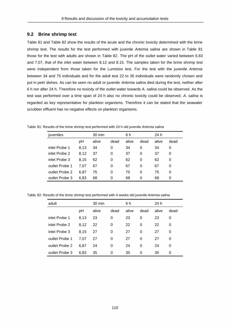
9 Results and discussion of the toxicity and accumulation tests
110
9.2 Brine shrimp test
Table 81 and Table 82 show the results of the acute and the chronic toxicity determined with the brine
shrimp test. The results for the test performed with juvenile Artemia salina are shown in Table 81
those for the test with adults are shown in Table 82. The pH of the outlet water varied between 6.83
and 7.07, that of the inlet water between 8.12 and 8.15. The samples taken for the brine shrimp test
were independent from those taken for the Lumistox test. For the test with the juvenile Artemia
between 34 and 75 individuals and for the adult test 22 to 35 individuals were randomly chosen and
put in petri dishes. As can be seen no adult or juvenile Artemia salina died during the test, neither after
6 h nor after 24 h. Therefore no toxicity of the outlet water towards A. salina could be observed. As the
test was performed over a time span of 24 h also no chronic toxicity could be observed. A. salina is
regarded as key representative for plankton organisms. Therefore it can be stated that the seawater
scrubber effluent has no negative effects on plankton organisms.
Table 81: Results of the brine shrimp test performed with 24 h old juvenile Artemia salina
juveniles 30 min 6 h 24 h
pH alive dead alive dead alive dead
inlet Probe 1 8,13 34 0 34 0 34 0inlet Probe 2 8,12 37 0 37 0 37 0
inlet Probe 3 8,15 62 0 62 0 62 0
outlet Probe 1 7,07 67 0 67 0 67 0
outlet Probe 2 6,87 75 0 75 0 75 0outlet Probe 3 6,83 68 0 68 0 68 0
Table 82: Results of the brine shrimp test performed with 4 weeks old juvenile Artemia salina
adult 30 min 6 h 24 h
pH alive dead alive dead alive dead
inlet Probe 1 8,13 23 0 23 0 23 0
inlet Probe 2 8,12 22 0 22 0 22 0
inlet Probe 3 8,15 27 0 27 0 27 0
outlet Probe 1 7,07 27 0 27 0 27 0
outlet Probe 2 6,87 24 0 24 0 24 0
outlet Probe 3 6,83 35 0 35 0 35 0
This document, and more, is available for download at Martin's Marine Engineering Page - www.dieselduck.net

9 Results and discussion of the toxicity and accumulation tests
111
9.3 Accumulation test
9.3.1 Mussel analyses: size, weight, condition index, fat content
In this chapter the results of the combined accumulation and toxicity test, performed with the mussel
Mytilus edulis, are presented. In Fig. 65 the proportions of the dry tissue, the shell weight and the
water content are shown. The sizes of the single mussels are shown in Table 83. “Control 2”
contained in comparison to “control 5” and “control 8” more individuals greater than 60 mm whereas in
“control 5” and “control 8” there were more individuals smaller than 50 mm. The water content and the
dry tissue weight of the latter two are with 26.9 %, 27.2 % and 4.5 %, 5.1%, respectively, higher than
in “control 2” with 23.7 % water content and 3.2 % dry tissue weight. A similar behaviour can be
observed for the tests “part 01”, “part 04” and “part 07”. In test “part 01” 11 mussels were greater than
or equal 60 mm, in “part 04” only 4 and in “part 07” none of the mussels was greater than 60 mm. For
the tests “diss 03”, “diss 06” and “diss 09” the size distributions were similar to those of the particulate
trial and the controls, with relatively more long mussels in trial “diss 03” and fewer in trial “diss 06” and
“diss 09”. In this case the observed relations of water, shell and dry tissue weight are only reflected in
the water content. On the right side of Fig. 65 the mean percentages of the water content, the dry
tissue and the shell weight of all size classes, are given. It can be seen that increasing mussel size is
paralleled by an increase in shell weight and a decrease in relative water content.
This document, and more, is available for download at Martin's Marine Engineering Page - www.dieselduck.net

9 Results and discussion of the toxicity and accumulation tests
112
Table 83: length [mm] of all mussels employed for the accumulation test. The colours separate the table in themain classes used for the PAH determination. The first class smaller than 50 mm and the second classbetween 50 mm and 60 mm
control externalbasin
part 01 cont 02 diss 03 part 04 cont 05 diss 06 part 07 cont 08 diss 09
15.2 36.2 36.1 31.1 40.2 41.8 35.6 40.1 38.8 43.415.8 38.4 36.1 36.8 41.7 44.8 42.5 42.9 41.4 43.722.4 39.4 36.7 38.9 42.2 45 43.3 44 41.8 46.724.7 40.1 38.2 40.8 43.2 45.4 43.4 44 42.7 49.128.2 41 39.3 43.8 43.8 46 43.9 44.1 43.7 49.233 44.8 47.8 46.9 43.9 46.4 44.1 45.6 45.5 49.933.3 45.8 47.8 49.2 44.7 46.7 44.5 45.6 46.1 50.339.1 51.5 49.5 50.4 45.7 47.2 46.1 46.1 46.4 50.945.3 52 53.2 52.9 46.1 47.4 46.5 46.3 47.2 52.145.3 53.5 53.4 53.3 46.3 47.8 47.3 47.4 47.6 52.846.4 54.1 54.9 53.9 47.2 47.9 47.4 47.8 47.8 5347.1 54.5 55.1 54.1 48.8 48.3 48.2 49.5 48.7 53.247.6 55.8 56 55.9 50.1 48.4 48.2 49.6 48.8 53.348.2 56.5 56.5 57.1 50.3 48.6 48.6 49.6 49 54.248.4 57.5 56.7 58 50.8 49.2 49 50.2 49.7 54.449.8 57.6 57.2 58.5 51.4 49.2 49.2 51.2 49.7 5550 59.8 58.2 59.2 51.6 49.2 49.2 51.3 49.8 55.350.2 59.9 58.5 61.1 52.4 50 49.9 51.7 50.4 56.350.3 60 59 61.3 52.7 50.7 50.7 52.1 50.7 56.750.8 60.1 59.1 61.3 55.2 51.5 51 52.3 51.8 56.851.6 61.2 59.2 61.5 55.2 52.1 51.5 52.5 52.3 5752.6 61.2 59.9 61.7 55.7 52.6 51.6 52.8 52.8 57.752.6 62 60.1 62.1 55.8 53.7 51.7 53.4 53.3 58.752.6 63.5 61.5 62.8 59.7 54.5 52.5 53.4 53.8 59.153.2 66 62 63 59.8 55.8 52.7 53.5 55.1 59.453.6 66.5 65.8 63.8 59.9 55.9 53.3 50 55.8 59.953.8 67.5 66.8 63.9 60.5 56.1 53.8 54.9 56.6 60.654.7 69.7 67.7 64.3 62.5 56.2 54.8 57.1 56.9 6156.3 70.2 69.6 63 59.4 56.3 59 60.8 62.256.5 68.9 70 56.7 62.856.656.857.758.462.86470.7
0%
10%
20%
30%
40%
50%
60%
70%
80%
90%
100%
17,0 25,6 35,7 45,8 54,5 63,3
mean length [mm]
per
cent
age
waterdry tissueshell
Fig. 65: Mean percentages of shell, dry and wet tissue weight for all mussels used in the accumulation test. Left:percentages for each test, right: mean for all tests.
This document, and more, is available for download at Martin's Marine Engineering Page - www.dieselduck.net

9 Results and discussion of the toxicity and accumulation tests
113
0
10
20
30
40
50
60
70
0 50 100
length [mm]
wh
ole
wet
wei
gh
t[g
]
0
10
20
30
40
50
60
70
0 50 100
length [mm]
shel
lw
eig
ht
[g]
Fig. 66: Correlation plots. Left: whole wet weight against length. Right: shell weight against length. In both casesthe red line shows the nonlinear model and the black lines the 95 % confidence interval
0
2
4
6
8
10
12
0 50 100
length [mm]
tis
sue
we
twe
ight
[g]
0
0,5
1
1,5
2
2,5
3
3,5
0 50 100
length [mm]
dry
tis
sue
[g]
00,2
0,40,6
0,81
1,21,4
1,6
1,8
0 5 10 15
wet tissue [mm]
dry
tiss
ue
[g]
Fig. 67: Correlation plots: Left: wet tissue weight against length. Middle: dry tissue weight against length. Right:dry tissue weight against wet tissue weight. In both cases the red line shows the nonlinear model andthe black lines the 95 % confidence interval
In Fig. 66 and Fig. 67 the correlation plots of total wet weight, shell weight, dry tissue weight, and wet
tissue weight against shell length and dry tissue against wet tissue weight are shown. The used model
functions, their parameters, the 95 % confidence intervals of the parameters and the correlation
coefficient R² are shown in Table 84. It can be seen that the dependencies between length and shell
weight, wet weight and total weight show good correlations, whereas the scatter of the dry tissue
weight is much higher.
Table 84: Results of linear and nonlinear regression
dependent variable weighttotal [g]
weightshell [g]
weightwet tissue [g]
weightdry tissue [g]
weightdry tissue [g]
independent variable length [mm] length [mm] length [mm] length [mm] weightdry tissue [g]
function bxay bxay bxay bxay xay Parameter a 6.732E-05 1.206E-05 2.332E-04 2.564E-04 0.1488min 95 % 4.700E-05 7.115E-07 1.200E-04 1.490E-05 0.1450max 95 % 8.800E-05 2.341E-05 3.465E-04 4.980E-04 0.1530Parameter b 3.062 3.363 2.412 1.910min 95 % 2.886 3.131 2.291 1.675max 95 % 3.238 3.595 2.533 2.145R² 0.826 0.767 0.874 0.551 0.753
This document, and more, is available for download at Martin's Marine Engineering Page - www.dieselduck.net

9 Results and discussion of the toxicity and accumulation tests
114
9.3.2 Mussel analyses: PAH content, accumulation, mortality
In Fig. 68 the results of the standardized mussel tissue extraction and the R² values for the calibration
lines are shown. The error bars for the mussel tissue are the errors given by the manufacturer. The
error bars of the determined values are calculated by aid of the GC-MS accuracy according to the
values given in Table 17 (25 µg l-1). It can be seen that all values were determined within the given
error range and accuracy with the exception of fluorene. In this case the determined concentration
was 11.3 ± 0.2 ng g-1 whereas the given value was 10.2 ± 0.4 ng g-1. It has to be considered, that only
the accuracy of the GC-MS measurement was stated and not the accuracy of the whole method,
which would be somewhat higher. For the mussel extraction the accuracy of the method was not
determined like for the extraction of the water samples, because a standardised reference material as
control was available.
All determined PAH concentrations are shown in Table 85. The compounds added permanently during
the test are indicated in italics. The contents of these compounds are also visualised in Fig. 69. The
“background” concentrations of those compounds that were not added during the test are shown in
Fig. 70. These contents can be regarded as negative control. In the latter graph it can be seen that
acenaphthylene, acenaphthene and dibenz[a,h]anthracene are equally concentrated in all mussels,
benzo[a]pyrene, benzo[ghi]perylene and indeno(1,2,3,c,d)pyrene are slightly increased and fluorene,
benz[a]anthracene and benzo[b]fluoranthene plus benzo[k]fluoranthene are nearly doubled in the
controls from the external basin. It can also be seen that within the external controls the PAH contents
are slightly increased in those mussels greater than 50 mm. For the mussels used in the test an
inverse distribution was observed. In most cases the concentration is lower in the mussels smaller
than 50 mm. Fig. 69 also shows a quite similar distribution of PAHs in the controls from the external
basin and from the controls in the test. The PAH concentrations of those compounds added
permanently are increased clearly in the mussels from the particulate and the dissolved test in
comparison to the controls and those mussels from the external basin. Comparing the results from the
dissolved and the particulate test there is no difference recognizable. To check this observation
statistically, a t-test was performed. The test was performed in two different ways: I) to check whether
there is a significant difference between the two size classes and II) to check whether there is a
significant difference between the dissolved and the particulate tests. The used test was the t-test for
testing the equality of the variances of two dependent random samples and was calculated according
to
222
21
22
21 14
2Rss
nsst
where s1 and s2 are the standard deviations of two samples, n is the number of compared rows and R²
is the correlation coefficient. The reference value can be taken from a significance chart (degrees of
freedom = 8, α= 5 %; t (8/0.05) = 2.31). In both cases the calculated t-value was below 2.31, therefore it
can be said that the observed differences in variability are coincidental. A measure for the correlation
can be given by the R² which is 0.9763 for the comparison of the PAH concentrations in the mussels
This document, and more, is available for download at Martin's Marine Engineering Page - www.dieselduck.net
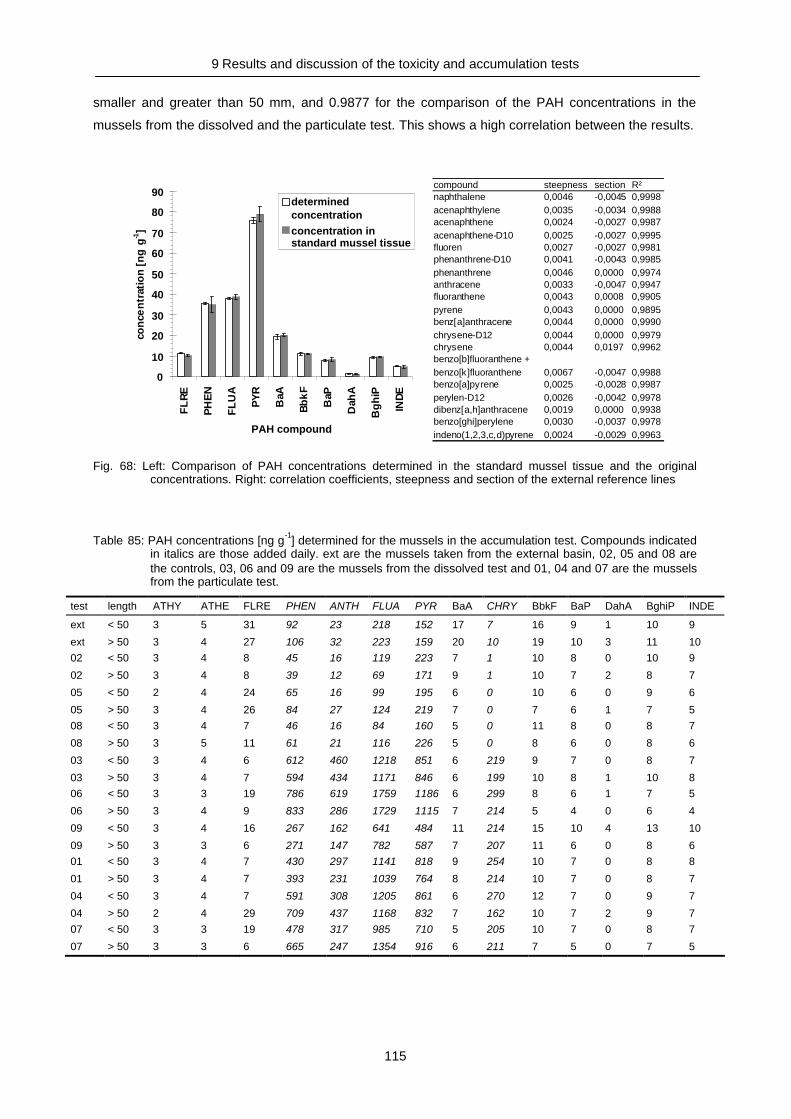
9 Results and discussion of the toxicity and accumulation tests
115
smaller and greater than 50 mm, and 0.9877 for the comparison of the PAH concentrations in the
mussels from the dissolved and the particulate test. This shows a high correlation between the results.
0
10
20
30
40
50
60
70
80
90F
LR
E
PH
EN
FL
UA
PY
R
BaA
Bb
kF
BaP
Dah
A
Bg
hiP
IND
E
PAH compound
con
cen
trat
ion
[ng
g-1]
determinedconcentrationconcentration instandard mussel tissue
compound steepness section R²naphthalene 0,0046 -0,0045 0,9998acenaphthylene 0,0035 -0,0034 0,9988acenaphthene 0,0024 -0,0027 0,9987acenaphthene-D10 0,0025 -0,0027 0,9995fluoren 0,0027 -0,0027 0,9981phenanthrene-D10 0,0041 -0,0043 0,9985phenanthrene 0,0046 0,0000 0,9974anthracene 0,0033 -0,0047 0,9947fluoranthene 0,0043 0,0008 0,9905pyrene 0,0043 0,0000 0,9895benz[a]anthracene 0,0044 0,0000 0,9990chrysene-D12 0,0044 0,0000 0,9979chrysene 0,0044 0,0197 0,9962benzo[b]fluoranthene +benzo[k]fluoranthene 0,0067 -0,0047 0,9988benzo[a]pyrene 0,0025 -0,0028 0,9987perylen-D12 0,0026 -0,0042 0,9978dibenz[a,h]anthracene 0,0019 0,0000 0,9938benzo[ghi]perylene 0,0030 -0,0037 0,9978indeno(1,2,3,c,d)pyrene 0,0024 -0,0029 0,9963
Fig. 68: Left: Comparison of PAH concentrations determined in the standard mussel tissue and the originalconcentrations. Right: correlation coefficients, steepness and section of the external reference lines
Table 85: PAH concentrations [ng g-1] determined for the mussels in the accumulation test. Compounds indicatedin italics are those added daily. ext are the mussels taken from the external basin, 02, 05 and 08 arethe controls, 03, 06 and 09 are the mussels from the dissolved test and 01, 04 and 07 are the musselsfrom the particulate test.
test length ATHY ATHE FLRE PHEN ANTH FLUA PYR BaA CHRY BbkF BaP DahA BghiP INDE
ext < 50 3 5 31 92 23 218 152 17 7 16 9 1 10 9
ext > 50 3 4 27 106 32 223 159 20 10 19 10 3 11 1002 < 50 3 4 8 45 16 119 223 7 1 10 8 0 10 9
02 > 50 3 4 8 39 12 69 171 9 1 10 7 2 8 7
05 < 50 2 4 24 65 16 99 195 6 0 10 6 0 9 6
05 > 50 3 4 26 84 27 124 219 7 0 7 6 1 7 508 < 50 3 4 7 46 16 84 160 5 0 11 8 0 8 7
08 > 50 3 5 11 61 21 116 226 5 0 8 6 0 8 6
03 < 50 3 4 6 612 460 1218 851 6 219 9 7 0 8 7
03 > 50 3 4 7 594 434 1171 846 6 199 10 8 1 10 806 < 50 3 3 19 786 619 1759 1186 6 299 8 6 1 7 5
06 > 50 3 4 9 833 286 1729 1115 7 214 5 4 0 6 4
09 < 50 3 4 16 267 162 641 484 11 214 15 10 4 13 10
09 > 50 3 3 6 271 147 782 587 7 207 11 6 0 8 601 < 50 3 4 7 430 297 1141 818 9 254 10 7 0 8 8
01 > 50 3 4 7 393 231 1039 764 8 214 10 7 0 8 7
04 < 50 3 4 7 591 308 1205 861 6 270 12 7 0 9 7
04 > 50 2 4 29 709 437 1168 832 7 162 10 7 2 9 707 < 50 3 3 19 478 317 985 710 5 205 10 7 0 8 7
07 > 50 3 3 6 665 247 1354 916 6 211 7 5 0 7 5
This document, and more, is available for download at Martin's Marine Engineering Page - www.dieselduck.net
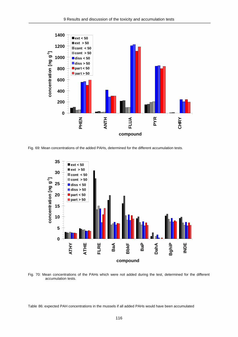
9 Results and discussion of the toxicity and accumulation tests
116
0
200
400
600
800
1000
1200
1400
PH
EN
AN
TH
FLU
A
PY
R
CH
RY
compound
con
cen
trat
ion
[ng
g-1]
ext < 50ext > 50cont < 50cont > 50diss < 50diss > 50part < 50part > 50
Fig. 69: Mean concentrations of the added PAHs, determined for the different accumulation tests.
0
5
10
15
20
25
30
35
AT
HY
AT
HE
FL
RE
BaA
Bb
kF
BaP
Dah
A
Bg
hiP
IND
E
compound
con
cen
trat
ion
[ng
g-1]
ext < 50ext > 50cont < 50cont > 50diss < 50diss > 50part < 50part > 50
Fig. 70: Mean concentrations of the PAHs which were not added during the test, determined for the differentaccumulation tests.
Table 86: expected PAH concentrations in the mussels if all added PAHs would have been accumulated
This document, and more, is available for download at Martin's Marine Engineering Page - www.dieselduck.net

9 Results and discussion of the toxicity and accumulation tests
117
PHEN ANTH FLUA PYR CHRYparticulate 01 <50 47926 20036 18668 8141 1399
>50 47926 20036 18668 8141 1399particulate 04 <50 47652 19921 18561 8095 1391
>50 47652 19921 18561 8095 1391particulate 07 <50 47199 19731 18385 8018 1378
>50 47199 19731 18385 8018 1378diss 03 <50 35501 14841 13828 6031 1037
>50 35501 14841 13828 6031 1037diss 06 <50 43475 18175 16934 7385 1269
>50 43475 18175 16934 7385 1269diss 09 <50 53405 22326 20802 9072 1559
>50 53405 22326 20802 9072 1559
Table 87: Percentage of accumulated PAHs, calculated as quotient of expected and observed PAH contents inthe mussels.
PHEN ANTH FLUA PYR CHRYparticulate 01 <50 0.9 1.5 6.1 10.0 18.2
>50 0.8 1.2 5.6 9.4 15.3particulate 04 <50 1.2 1.5 6.5 10.6 19.4
>50 1.5 2.2 6.3 10.3 11.6particulate 07 <50 1.0 1.6 5.4 8.9 14.9
>50 1.4 1.3 7.4 11.4 15.3diss 03 <50 1.7 3.1 8.8 14.1 21.1
>50 1.7 2.9 8.5 14.0 19.2diss 06 <50 1.9 1.6 10.2 15.1 16.8
>50 1.9 1.6 10.2 15.1 16.8diss 09 <50 0.5 0.7 3.8 6.5 13.2
>50 0.5 0.7 3.8 6.5 13.2
During the whole test (30 days) the mussels in the dissolved and particulate trials were fed with the
following absolute PAH amounts:
phenanthrene = 640475 ng anthracene = 267750 ng fluoranthene = 249475 ng pyrene = 108800 ng chrysene = 18700 ng
Y
If the mussels would have accumulated the total amount of the added PAHs the concentration shown in Table 86would have to be expected. The values were calculated as the quotients of the total amount of the PAHcompounds and the sum of the dry tissue weight of all mussels used in the concerning test. Comparingthese values with the actually determined compound concentrations, the accumulation rate can becalculated, as quotient of the observed concentration and the expected concentration in percent. Theresults are shown in
Table 87. It can be seen that from the added phenanthrene 0.5 % to 1.9 %, the anthracene 0.7 % to
3.1 %, fluoranthene 3.8 % to 10.2 %, the pyrene 6.5 % to 10.6 % and the chrysene 11.6 % to 21.1 %
were accumulated.
This document, and more, is available for download at Martin's Marine Engineering Page - www.dieselduck.net

9 Results and discussion of the toxicity and accumulation tests
118
control - phenanthrene
0
50
100
150
200
250
300
begin end
conc
entr
atio
n[n
gl-1
]dissolved - phenanthrene
0
50
100
150
200
250
300
begin end
conc
entr
atio
n[n
gl-1
]
particulate - phenanthrene
0
50
100
150
200
250
300
begin end
conc
entr
atio
n[n
gl-1
]
control - anthracene
050
100150200250300350400450
begin end
conc
entr
atio
n[n
gl-1
]
2.7 2.2
dissolved - anthracene
050
100150200250300350400450
begin end
conc
entr
atio
n[n
gl-1
]
11.4 22.5
particulate - anthracene
050
100150200250300350400450
begin end
conc
entr
atio
n[n
gl-1
]
9.6
control - fluoranthene
0
200
400
600
800
1000
begin end
conc
entr
atio
n[n
gl-1
]
dissolved - fluoranthene
0
200
400
600
800
1000
begin end
conc
entr
atio
n[n
gl-1
]
particulatel - fluoranthene
0
200
400
600
800
1000
begin end
conc
entr
atio
n[n
gl-1
]
control - pyrene
0
200
400
600
800
1000
1200
begin end
conc
entr
atio
n[n
gl-1
]
dissolved - pyrene
0
200
400
600
800
1000
1200
begin end
conc
entr
atio
n[n
gl-1
]
particulate - pyrene
0
200
400
600
800
1000
1200
begin end
conc
entr
atio
n[n
gl-1
]
control - chrysene
0
100
200
300
400
500
600
begin end
conc
entr
atio
n[n
gl-1
]
dissolved - chrysene
0
100
200
300
400
500
600
begin end
conc
entr
atio
n[n
gl-1
]
particulate - chrysene
0
100
200
300
400
500
600
begin end
conc
entr
atio
n[n
gl-1
]
particulatedissol
Fig. 71: Concentrations of phenanthrene, anthracene, fluoranthene, pyrene and chrysene [ng l-1] measured in theaquaria of the controls, the particulate and the dissolved test one hour after a water exchange and rightbefore the following water exchange (3 days). Contents are separated into dissolved and particulatefractions.
This document, and more, is available for download at Martin's Marine Engineering Page - www.dieselduck.net

9 Results and discussion of the toxicity and accumulation tests
119
During the accumulation test the contents of the added PAH compounds phenanthrene, anthracene,
fluoranthene, pyrene and chrysene in the water of the aquarium were determined half an hour after a
water exchange and directly before the following water exchange after three days. The results are
shown in Fig. 71. The pH, salinity and the water temperature are shown in Table 88. Within the water
samples of the controls the phenanthrene and anthracene contents were equally low in the beginning
and at the end of the three day period whereas the pyrene, chrysene and fluoranthene increased
during that time. The same was observed in the samples from the aquaria of the dissolved test. Also
the contents were quite similar. In contrary to the increase of dissolved pyrene, chrysene, and
fluoranthene, the contents observed in the particulate test showed another distribution: the
phenanthrene content in the beginning was 259 ng l-1 and in the end 15 ng l-1, the anthracene contents
were 427 ng l-1 and 10 ng l-1 the fluoranthene contents 727 ng l-1 and 174 ng l-1, the pyrene contetnts
609 ng l -1 and 203 ng l-1 and the chrysene contents 448 ng l-1 and 400 ng l-1, respectively. The
observed differences between the PAH contents of the particulate and the dissolved tests and the
increase of fluoranthene cannot be explained. One reason might be that the water of the aquarium
was not mixed thoroughly enough before taking the samples. This was difficult as stirring was not
possible because of the mussels in the aquarium. This would also explain why mainly dissolved PAHs
were determined whereas the particulate PAH fraction was low. The reason for the latter aspect could
also be that the samples were not taken directly after the PAH addition, but about half an hour later.
As blue mussels are able to filter about 1 l seawater per hour and 30 mussels were inside the
aquarium half an hour would be sufficient to filter the whole water volume of 17 l.
Table 88: pH, salinity and temperature determined in the aquariums during the test
pH Sal Temp [°C]1 7.91 31.5 18.52 8.06 31.5 18.53 7.83 31.5 18.54 7.92 31.5 18.35 8.01 31.5 18.56 7.94 31.5 18.47 7.94 31.5 18.58 8.02 31.5 18.59 7.93 31.5 18.5
From Table 77 where the PAH concentrations determined for the mussels taken in Calais are shown.
It can be seen that the total amount of the mussels smaller than 40 mm in Calais is about the same as
those concentrations observed in the external basin and the controls, but the composition is different.
The mussels taken in Calais contain higher concentrations of phenanthrene and fluoranthene whereas
the mussel taken from the Jade Bay show higher concentrations of high molecular weight PAHs. Due
to their life history the mussels are not directly comparable concerning to their PAH concentrations.
The mussels in Calais were growing inside an enclosed harbour with high shipping activities. The PAH
composition of this harbour has been discussed before. The mussels taken from the Jade Bay were
mainly influenced from PAHs reaching them through the atmosphere. Therefore they contain mainly
high molecular weight PAHs.
This document, and more, is available for download at Martin's Marine Engineering Page - www.dieselduck.net

9 Results and discussion of the toxicity and accumulation tests
120
Although the PAH compositions of the mussels cannot be compared directly, the accumulation rates will besimilar. The „Pride of Kent“ discharges about 52.5 m³ of mixed colling water/seawater scrubbereffluents during each visit (see 8.6.4 on page 100) in the ports of Dover and Calais, 5 times a day.During one day 252.5 m³ of outlet water would be introduced into each port. Taking the mean PAHdifferences of Table 73 this would sum up to a total PAH introduction and to a concentration increaseof the values shown in Table 89. As only the water volume of the port of Dover was available thiscalculation was exemplary carroied out with this volume (2.538 km²). In this calculation losses due tobiological or chemical degradation (UV, micro organisms, translocation processes) and physicalprocesses (currents, adsorption and settling) are not included. Assuming that one mussel filters about1 l seawater per hour and using the dry weight calculated according to Table 84 and a meanaccumulation rate from
Table 87 then the contents given in Table 90 would be the result after one year of accumulation for
one mussel. As inside a harbour there is not only one mussel and as the accumulated PAHs would
have to be subtracted from the available PAHs in the water body the real value makes up only a very
small fraction of the values in shown in Table 90.
Table 89: Total PAH amounts [mg] that will be theoretically introduced during one day into the ports of Dover andCalais and theoretical concentration increase [pg l-1]
total amount [mg]released in 1 day
concentration increase[pg l-1] per day
ATHY 1 1ATHE 6 3FLRE 34 13PHEN 296 117ANTH 7 3FLUA 45 18PYR 103 41BaA 66 26CHRY 95 37BbkF 15 6BaP 33 13DahA 5 2BghiP 11 4INDE 4 2
Table 90: Mean accumulation rate, total accumulation per day and year and resulting contamination after oneyear for a 20 mm mussel.
mean accrate [%]
accumulationper day [pg]
accumulationper year [ng]
concentration in a 20 mmmussel after 1 year [ng g-1]
1.3 35 12.8 1631.7 1 0.4 56.9 29 10.6 13611.0 107 39.1 49916.3 102 37.2 475
Mortality
This test was also performed as a toxicity test. Therefore the mortality of the mussels was also
observed. During the whole test 4 of the 270 employed mussels died. Two mussels of the aquarium
“diss 3” after three and after 21 days, one of test “part 7” after seven days and one in aquarium “part
1” after 10 days. As the mussels of the particulate and the dissolved test were equally contaminated
with PAHs this mortality can be assumed for all mussels in the tests. Four mussels of the 180 mussels
This document, and more, is available for download at Martin's Marine Engineering Page - www.dieselduck.net
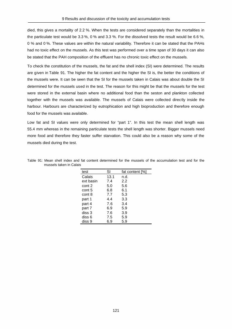
9 Results and discussion of the toxicity and accumulation tests
121
died, this gives a mortality of 2.2 %. When the tests are considered separately than the mortalities in
the particulate test would be 3.3 %, 0 % and 3.3 %. For the dissolved tests the result would be 6.6 %,
0 % and 0 %. These values are within the natural variability. Therefore it can be stated that the PAHs
had no toxic effect on the mussels. As this test was performed over a time span of 30 days it can also
be stated that the PAH composition of the effluent has no chronic toxic effect on the mussels.
To check the constitution of the mussels, the fat and the shell index (SI) were determined. The results
are given in Table 91. The higher the fat content and the higher the SI is, the better the conditions of
the mussels were. It can be seen that the SI for the mussels taken in Calais was about double the SI
determined for the mussels used in the test. The reason for this might be that the mussels for the test
were stored in the external basin where no additional food than the seston and plankton collected
together with the mussels was available. The mussels of Calais were collected directly inside the
harbour. Harbours are characterized by eutrophication and high bioproduction and therefore enough
food for the mussels was available.
Low fat and SI values were only determined for “part 1”. In this test the mean shell length was
55.4 mm whereas in the remaining particulate tests the shell length was shorter. Bigger mussels need
more food and therefore they faster suffer starvation. This could also be a reason why some of the
mussels died during the test.
Table 91: Mean shell index and fat content determined for the mussels of the accumulation test and for themussels taken in Calais
test SI fat content [%]Calais 13.1 n.d.ext basin 7.4 2.2cont 2 5.0 5.6cont 5 6.8 6.1cont 8 7.7 5.3part 1 4.4 3.3part 4 7.6 3.4part 7 6.9 5.9diss 3 7.6 3.9diss 6 7.5 5.9diss 9 6.9 5.9
This document, and more, is available for download at Martin's Marine Engineering Page - www.dieselduck.net

10 Conclusions
122
10 Conclusions
During this project the environmental impact of a seawater scrubber has been analysed for the
harbours of Calais and Dover. Five sampling campaigns were organised during which samples were
taken inside the ports, from the seawater scrubber system and within a transect leading 700 m away
from the seawater scrubber outlet. The seawater scrubber, the so-called “Ecosilencer”, was installed
in the funnel of the channel ferry “Pride of Kent” to reduce her SOx emissions. As seawater scrubbing
is a wet fluegas desulphurisation process not only SOx is dissolved but also NOx, volatile organic
compounds, and hydrochloric acid. The dissolved SOx and NOx form sulphuric and nitric acids and
reduce together with the HCl the pH of the scrubbing effluent significantly. The samples taken from the
seawater scrubber system partially showed pH values lower than pH 3. Because of the buffering
capacity of seawater due to the bicarbonate system the pH increases again after an initial acidification.
This could be shown in several experiments. From these it could also be shown that a mixture
containing 40 % of seawater acidified to a pH of 4, i.e. comparable to that what happens in a seawater
scrubber, only changes its pH about 0.2 units. To reach this equilibrium several hours were needed
but the largest changes were observable already a short time after mixing. On board of the „Pride of
Kent“ the seawater scrubber effluent was mixed with seawater from the cooling cycle of the vessel.
Thus a significant pH increase could be obtained but the pH was still lower in comparison to the inlet
and the surrounding waters. The lowest pH measured in the overboard discharge was 6.2. As many
organisms are only able to survive when environmental conditions are stable adecrease in pH might
be a risk for those organisms. That is why the United States Environmental Protection Agency has
passed a guideline concerning the introduction of acids which states that within the initial mixing zone
the pH change is not allowed to be higher than 0.2 units. In the case of the Ecosilencer the initial
mixing zone is directly in front of the overboard discharge of the „Pride of Kent“. To check whether
there is an observable pH change, samples were taken directly in front of the outlet (1 to 5 m distance)
and 50 m, 350 and 700 m away from the outlet. In no sample taken at the first point of this transect a
pH decrease was observed. In Calais the natural pH variability was much higher than the variability
measured in the transect. This shows that the bicarbonate system in the seawater effectively buffers
the acids added by the operation of the Ecosilencer.
Additionally to the acidification the dissolved SOx increases the sulphate concentration in the effluent.
The samples taken behind the Ecosilencer showed a sulphate increase between 14.0 and 18.7 %. In
fresh water lakes sulphate might be a limiting factor but in sea water sulphate is a common and
conservative component. The inlet samples taken in the Channel can be considered as blank sample,
because the inlet water was not influenced by the outlet water and in the Channel the water current is
high enough so that an influence of the previous passing of the „Pride of Kent“ can be neglected. In
these samples sulphate concentrations between 2590 and 2990 ppm were observed. In the outlet
samples values between 2600 and 3052 ppm were determined which accounts for an increase of 0.4
to 4.5 %. As the method to determine this concentration already had an error of 6 % a sulphate
increase in the outlet samples cannot be stated for sure. Even if there would be a slight increase the
This document, and more, is available for download at Martin's Marine Engineering Page - www.dieselduck.net

10 Conclusions
123
influence of the seawater scrubber on the sulphate concentrations in the harbours and therefore on
the marine environment would be very low. Additionally it has to be mentioned that in Calais a wide
range of sulphate concentrations, between 1479 and 2628 ppm, was observed.
Another nutrient that might be influenced by the seawater scrubber is nitrate. It is formed in the
scrubbing process when NOx is dissolved in water. It is an important nutrient in the sea. In the samples
taken after the Ecosilencer in the Channel, the nitrate concentrations were about two to thirteen times
higher than in the seawater inlet samples. The cleanup processes on board (cyclones and US filter)
did not reduce these concentrations. The only reduction was observed after dilution of the effluent
water with the cooling water. In the effluent samples the nitrate was only twice the inlet concentration.
To determine the influence of this additionally added nitrogen a calculation was made to determine the
amount of additional biomass production. This showed that an increase in primary production in a
given year would be less than the actual primary production during one sunny day per square metre.
Another indirect influence of the seawater scrubber that has to be considered is that the reduced pH in
the effluent influences the solubility of metal ions. To check this, samples were taken from the
seawater scrubber system and analysed for their metal contents. The highest values for all samplings
were determined for the samples taken from the settling tank and the pipe leading to the settling tank.
This water contains the particles filtered from the water by the cyclones. The high concentrations
showed that the cyclones effectively remove contaminated particles. The highest metal contents were
determined for iron. As iron is the major compound of ship steel this result is not surprising. In the
outlet samples beside iron also copper, nickel and lead were found. These were only detected during
two samplings and here also in the inlet samples. The copper might originate from ship coatings that
contain copper as antifouling biocide while nickel is like iron a compound of ship steel. With respect to
the metals it can be said that the seawater scrubbing process itself has no influence on their contents,
but that due to the reduced pH metals are leached from the steel, the tubing and the funnel. If the
metals are present in particulate form they are filtered out of the water and retained in the settling tank.
The sludge is removed separately and therefore no harm on the marine environment is expected.
Another group of compounds that is enriched in the seawater scrubber effluent are polycyclic aromatic
hydrocarbons. These are either dissolved or bound to soot particles which are formed during
incomplete combustion processes. The low molecular weight PAHs such as the two and three ring
compounds are soluble in water whereas the higher molecular weight PAHs with four rings and more
are mainly bound to particles. Therefore not all PAHs can be removed from the water with the US filter
and the cyclones which remove only particulates. This is the reason why there were still relatively high
amounts of PAHs in the outlet samples. However, in front of the seawater scrubber outlet no
increased PAH contents could be determined. In Dover high PAH concentrations were most often
found close to the middle or in the western part of the port where the water is shallower. At this point
the current speeds are lower and therefore pollutants might be enriched. Close to the berth and at the
eastern entrance of the harbour low PAH contents were measured most probably originating from
North Sea water, which is lower contaminated with PAHs, and is flowing into the port at this point.
This document, and more, is available for download at Martin's Marine Engineering Page - www.dieselduck.net

10 Conclusions
124
In Calais the PAH contents were mostly equal at all points. Only during the sampling in March very
high contents were observed at point Cal 3. Here a total PAH content of 765 ng l-1 was measured
which was the highest value determined in all harbour samples. This high concentration was the result
of an algal bloom occurring at that point. The plankton cells might have enriched the PAHs by different
pathways: the PAHs might have adsorbed to the surface of the cells or the organism itself produced
the PAHs or took them up and accumulated them that way. This shows that there are also very high
natural variations. Seasonal variations were also observed. In summer the concentrations were close
to the detection limit and high molecular weight PAHs were not found at any point. In contrary in late
fall and early spring the PAH contents were higher. This variability is the result of fossil fuel burning
which is increased during the heating period. This is also the reason why in fall higher amounts of high
molecular weight PAHs were measured.
To determine the origin of the PAHs and to exclude the seawater scrubber as probable source
regression and principle component analyses were performed and different indices based on isomeric
ratios were applied. The latter indicated that the PAHs determined in the seawater scrubber samples
originated from a petrogenic source. This was surprising because it can be expected that in a funnel
only PAHs of pyrolytic origin should occur. The reason could be that the fuel is not completely
combusted. The indices calculated for the harbour samples did not clearly differentiate between a
pyrolytic or a petrogenic origin possibly due to the different PAH sources that influence the harbour.
On one hand there are big cities close to the ports introducing a high amount of PAHs originating from
a pyrolytic origin (shipping, car traffic, heating) and on the other hand there are the shipping activities
inside the port that introduce PAHs originating from petrogenic sources. With the linear regression and
the principle component analyses it could be shown that the composition of the seawater scrubber
samples was different from those observed in the harbours. A change of the signal due to the dilution
with the cooling water could be rejected because the PAHs in the outlet samples showed the same
distribution as those in the system itself. As data on seawater samples are rarely available in the
literature sediment and mussel samples were also taken inside the ports of Dover and Calais. The
PAH load of the sediments was comparable to concentrations measured in another French harbour
and were lower than in the ports with high shipping activities like Rotterdam and Amsterdam. The
mussels were higher contaminated than mussels collected at the Shetlands or in the Baltic.
With respect to temperature, nutrients and PAHs, the two ports showed differences. One reason might
be the different architecture. In Calais the harbour is enclosed by walls and is made up of three arms.
One arm is separated by a flood gate which is only opened during high tide. The city of Calais and
local industry are located next to the harbour and therefore the anthropogenic influence is relatively
high. A water exchange is only possible through a relatively small entrance in the north-west of the
harbour. In contrary the harbour of Dover possesses two entrances, one in the south and one in the
west. This enables a higher water exchange and therefore the water remains inside the harbour for a
shorter time. This port has no side arms where water can be retained, as the harbour walls are built
around a large basin. Due to this architecture the city of Dover touches the port only at the north side.
Because of these differences the environmental parameters determined in the ports were also
different. In Dover the salinity was higher and the water temperature was lower in the most cases than
This document, and more, is available for download at Martin's Marine Engineering Page - www.dieselduck.net
10 Conclusions
125
in Calais. Also the phosphate and nitrogen concentrationsn and in most cases also concentrations of
polycyclic aromatic hydrocarbons were lower. The nitrate concentrations determined for the two ports
showed a distinct seasonal behaviour. In summer low concentrations were measured, whereas in
February and November relatively high concentrations were observed. Nitrate is a limiting nutrient for
marine organisms and therefore it is depleted in summer when plankton bioproduction is high. In fall
and winter organic nitrogen compounds are remineralised and hence the nitrate concentrations
increase.
Additionally to the observations inside the ports and board of the „Pride of Kent“, toxicity tests were
performed to determine the overall toxicity of the outlet water. The tests covered inhibition of bacterial
luminescence, mortality of brine shrimps and accumulation of PAH by blue mussels (Mytilus edulis).
None of all this tests did reveal an increased toxicity of the effluent, neither acute nor chronic.
Summarizing the results it can be said that in the effluent the pH was decreased by a maximum of two
pH units, the sulphate content was slightly increased and the nitrate concentration was doubled. Close
to the seawater outlet in the ambient warters no decrease in pH, no higher nitrate or sulphate values,
and no increased PAH or metal contents were determined. Also no toxicity towards bacteria,
zooplankton or mussels was determined for the outlet samples. Although the PAHs are increased in
the outlet water these would have reached the North Sea anyway by atmospheric deposition after
release by combustion. In this case the PAH amounts would have been higher as in the seawater
scrubber system a part was collected by the cyclones. Improvement of the cylone efficiency would
help to minimise the problem of particulate PAH introduction to the marine environment
Additionally it has to be stated that when the seawater scrubber is to be be used in areas with brackish
or fresh waters, the effects might be different. Fresh waters have for example less pH buffering
capacitiy – unless the water drains a carbonaceous area - and therefore the critical load for acidity
might be reached very fast.
This document, and more, is available for download at Martin's Marine Engineering Page - www.dieselduck.net

References
126
References
Adami P, Barbieri P., Piselli S., Predonzani S., Reisenhofer E., 2000, Detecting and characterisingsources of persistent organic pollutants (PAHs and PCBs) in surface sediments of anindustrialized area (harbour of Trieste, northern Adriatic Sea)
Agency for toxic substances and disease registry (ATSDR), U.S. Department of health and humanservices, 1995, Toxicological profile for polycyclic aromatic hydrocarbons,http://www.atsdr.cdc.gov/toxprofiles/tp69.pdf
Agilent Technologies: Prest H., Solid-phase Extraction and Retention-Time Locked GC/MS Analysis ofSelected Polycyclic Aromatic Hydrocarbons (PAHs), Agilent Technologies, Inc, 1601 CaliforniaAve, Palo Alto, CA 94304, USA
Ahrens M. J., Depree C. V., 2004, Inhomogeneous distribution of polycyclic aromatic hydrocarbons indifferent size and density fractions of contaminated sediment from Auckland Harbour, NewZealand: an opportunity for mitigration, Marine Pollution Bulletin, Vol. 48 (2004) 341-350
Ankley G.T., Collyard S.A., Monson P.D., Kosian P.A. 1994. Influence of ultraviolet light on the toxicityof sediments contaminated with polycyclic aromatic hydrocarbons. Environmental toxicologyand chemistry, Vol. 13, pp.1791-1796.
Behrends B., Liebezeit G., 2003, Reducing SOX and NOX Emissions from Ships by a SeawaterScrubber, BP Marine Report, pp. 34.
Bispo A., Jourdain M.J., Jauzein M., 1999, Toxicity and genotoxicity of industrial soils polluted bypolycyclic aromatic hydrocarbons (PAHs), Organic Geochemistry, Vol. 30 (1999) 947-952
Capaldo K., Corbett J.J. ,Kasibhatla P., Fischbeck P., Pandis S.N., (1999), Effects of ship emissionson sulphur cycling and radiative climate forcing over the ocean, Nature, Vol. 400, 19 August1999
Corbett J.J., Koehler H.W., 2003, Update emissions from ocean shipping, Journal of GeophysicalResearch, Vol. 108, No D20, 4650
Council Directive 1999/30/EC of 22 April 1999 relating to limit values for sulphur dioxide, nitrogendioxide and oxides of nitrogen, particulate matter and lead in ambient air; OJ L 31313/12/2000 p.12
Council Directive 1999/32 relating to a reduction in the sulphur content of certain liquid fuels andamending Directive 93/12/EEC; OJ L 121, 11.5.99 p.13
Crozier, P. W., PlomLey J. B., Matchuk L., 2001, Trace level analysis of polycyclic aromatichydrocarbonsin surface waters by solid phase extraction (SPE) and gas chromatography-iontrap mass spectrometry (GC-ITMS), The Analyst, 126, 1974-1979
de Boer J., van der Zande T.E., Pieters H., Ariese F., Shipper C.A., van Brummelen T., Vethaak A.D.,Organic contaminants and trace metals in flounder liver and sediment from the Amsterdamand Rotterdam habours and off the Dutch coast, 2001, Journal of Environmental Monitoring, 3pp.386-393
Directive 2001/81/EC of the European Parliament and of the Council of 23 October 2001 on nationalemissions ceilings for certain pollutants OJ L 309 27/11/2001 p.1
Doong R.A., Lin Y.T., 2004, Characterisation and distribution of polycyclic aromatic hydrocarboncontamination in surface sediment and water from Gao-ping River, Taiwan. Water Research,Vol. 38(7), pp 1733-44
This document, and more, is available for download at Martin's Marine Engineering Page - www.dieselduck.net