EFFECTS OF NATIONAL NEWSPAPER ADVERTISING …

EFFECTS OF NATIONAL NEWSPAPER ADVERTISING EXPENDITURES ON

AGGREGATE CONSUMPTION

by

J. WESLEY BURNETT

(Under the Direction of Hugh J. Martin)

ABSTRACT

This study extends the academic community’s understanding of the macroeconomic

effects of advertising by examining the relationship between aggregate consumption and

newspaper advertising expenditures. The study found three things: (1) aggregate consumption

Granger-causes newspaper advertising expenditures; (2) changes to newspaper advertising

expenditures and aggregate consumption are disproportionate; and (3) changes to newspaper

advertising expenditures do not lag behind changes to aggregate consumption but rather occurs

concurrently.

INDEX WORDS: Economics of Advertising, Macroeconomic Effects of Advertising,

Advertising Expenditures, Aggregate Consumption



by

J. WESLEY BURNETT

BA, College of Charleston, 1999

A Thesis Submitted to the Graduate Faculty of The University of Georgia in Partial Fulfillment

of the Requirements for the Degree

MASTER OF ARTS

ATHENS, GEORGIA

2007

© 2007

J. Wesley Burnett

All Rights Reserved



by

J. WESLEY BURNETT

Major Professor: Hugh J. Martin

Committee: Dean Krugman

Ann Hollifield

Christopher Cornwell

Electronic Version Approved:

Maureen Grasso

Dean of the Graduate School

The University of Georgia

August 2007

iv

DEDICATION

I would like to dedicate this work to my endearing wife who has been so supportive

throughout this entire process.

v

ACKNOWLEDGEMENTS

I would like to acknowledge the assistance of my thesis committee—Dr. Hugh J. Martin,

Dr. Ann Hollifield, Dr. Dean Krugman, and Dr. Christopher Cornwell. Each of these persons

contributed their expertise, without which this work would be nowhere near complete. I would

like to especially acknowledge my major professor Dr. Hugh J. Martin whose mentorship and

insightfulness made this process truly fulfilling.

vi

TABLE OF CONTENTS

Page

ACKNOWLEDGEMENTS.............................................................................................................v

LIST OF TABLES........................................................................................................................ vii

LIST OF FIGURES ....................................................................................................................... ix

CHAPTER

1 INTRODUCTION .........................................................................................................1

2 LITERATURE REVIEW ..............................................................................................3

Development of Microeconomic Models of Advertising..........................................3

Empirical Evidence of Advertising Effects on the Economy at the Macro-level ...12

Advertising Issues in Marketing Research..............................................................16

3 HYPOTHESIS AND METHODOLOGY ...................................................................22

Hypotheses ..............................................................................................................22

Methodology ...........................................................................................................23

Data .........................................................................................................................25

4 RESULTS ....................................................................................................................31

5 CONCLUSION............................................................................................................55

REFERENCES ..............................................................................................................................59

FOOTNOTES ................................................................................................................................63

vii

LIST OF TABLES

Page

Table 1.1: Annual Newspaper Advertising Expenditures as a Percentage of National Advertising

Expenditures ...................................................................................................................28

Table 1.2: Annual Newspaper Advertising Expenditures as a Percentage of National Advertising

Expenditures ...................................................................................................................29

Table 2.1: Descriptive Statistics of Percentage Changes in Newspaper Ad Expenditures and

Aggregate Consumption .................................................................................................32







Table 3: Augmented Dickey-Fuller Test for Unit Root in Aggregate Consumption ....................39

Table 4: Augmented Dickey-Fuller Test for Unit Root in News Advertising Expenditures.........39

Table 5: Augmented Dickey-Fuller Test for Unit Root in the First Difference of Aggregate

Consumption...................................................................................................................40

Table 6: Augmented Dickey-Fuller Test for Unit Root in the First Difference of News

Advertising Expenditures................................................................................................40

Table 7: Granger Causality Testing Results ..................................................................................46

viii

Table 8.1: Proportionality of Change Between National Ad Expenditures and Aggregate

Consumption...................................................................................................................47

Table 8.2: Proportionality of Change Between National Ad Expenditures and Aggregate

Consumption...................................................................................................................48

Table 9.1: The First Differences in Aggregate Consumption and Advertising Expenditures .......49




ix

LIST OF FIGURES

Page

Figure 1: Log of Aggregate Consumption Plotted Against Time..................................................37

Figure 2: Log of Newspaper Advertising Expenditures Plotted Against Time .............................38

Figure 3.1: Overlaid Graph of the Difference of the Log of Aggregate Consumption and the

Difference of the Log of News Ad Expenditures Plotted Against Time; Observations

1 - 35..............................................................................................................................41



36 - 71............................................................................................................................42



72 - 107..........................................................................................................................43



108 - 140........................................................................................................................44



70-80..............................................................................................................................45

1

CHAPTER 1

INTRODUCTION

This study will address one of the less understood questions in the field of advertising—

does advertising affect the general economy? Many studies (Marshall, 1920; Chamberlin, 1933;

Robinson, 1936; Kaldor, 1950; Galbraith, 1958; Comanor & Wilson, 1967) about the economic

consequences of advertising exist at the microeconomic level, including advertising’s effects on

industry profits and concentration, the impact of advertising on manufacturing and retail prices,

and advertising’s effects on the height of barriers to entry (Farris & Albion, 1980). However, the

impact of advertising at the macroeconomic level has been less explored. In fact, to the best of

the author’s knowledge, there are no macroeconomic models that explain advertising’s effects on

the national economy.

Despite the lack of theoretical attention to the macroeconomic effects of advertising,

empirical evidence does exist. Modern mass communication scholars found advertising has a

positive correlation with gross domestic product (Picard, 2001; Chang & Chan-Olmstead, 2005).

However, it is difficult to interpret the meaning of the positive correlation because numerous

economists have engaged in a still unresolved debate about advertising’s micro-level effects. For

instance, economists argued that advertising creates monopoly powers for the advertiser

(Marshall, 1919; Chamberlin, 1953; Robinson, 1936; Kaldor, 1950; Galbraith, 1958; Comanor &

Wilson, 1967). Arguments that advertising does not increase economic or social welfare trace

back to neoclassical economics (Ekelund & Saurman, 1988). But modern or new neoclassical

economists argue for positive effects of advertising on the economy (Ekelund & Saurman, 1988).

Despite more than 50 years of research, the debate is unresolved. This lack of understanding

lends to the need for continued research.

2

This thesis seeks to add to the sparse literature in one area of the debate by examining the

macroeconomic effects of advertising on the national economy. At the national level,

advertising arguably only has an effect on aggregate consumption (Ekelund & Gramm, 1969).

Therefore, this study will utilize quarterly, aggregate consumption data. The thesis will examine

the relationship between consumption and quarterly spending on advertising. Specifically, this

thesis will revisit an earlier project by Ashley, Granger, and Schmalensee (1980) in which the

authors tested whether national advertising expenditures Granger-cause national aggregate

consumption. Since the (Ashley et al., 1980) study, only one additional research endeavor was

found in the economics literature that concerned the aggregate consumption—national

advertising question. However, the most recent study (Jung & Seldon, 1995) dedicated to this

question utilized annual data which does not appropriately capture the dynamic effects of

quarterly changes to advertising expenditures. Therefore, this thesis extends the research

regarding aggregate consumption and national advertising by utilizing quarterly advertising data.

The results of this thesis will help the academic community better understand the

macroeconomic effects of advertising. The author hopes this study will prompt the academic

community to develop a macroeconomic model explaining how advertising affects the national

economy, but such an endeavor is beyond the scope of the current project.

3

CHAPTER 2

LITERATURE REVIEW

Development of Microeconomic Models of Advertising

One of the first economists to discuss advertising was the neoclassicist Alfred Marshall.

Marshall refers briefly to advertising in several sections of his seminal work Principle of

Economics (1920). He writes that a sufficiently large producer can take advantage of economies

of scale by advertising to increase market share: “[the producer] can spend large sums on

advertising by commercial traveler and in other ways; its agents give it trustworthy information

on trade and personal matters in distant places…” (Marshall, 1920, p. 282). Marshall discusses

how advertising can also increase the life of a business beyond the stage of natural decay within

its lifecycle (1920, p. 286). Marshall also recognizes how advertising and marketing expenses

are often necessary costs in the operation of business, especially businesses that do not operate in

perfectly competitive markets (1920, p. 396). Marshall posits that advertising and marketing can

help a producer cover some variable costs by selling surplus output in other markets (1920, pp.

457-458). Therefore, it seems at first that Marshall considered advertising a necessary part of the

economic process. However, Marshall elucidates his view of the effectiveness of advertising in

“Industry and Trade” (1927). Marshall claims wealthy producers have the ability to oust

competition through advertising, which he calls “social waste” (p. 306-307). Another element of

social waste is when advertising by wealthier producers throws into obscurity the advertisements

from less wealthy producers (Marshall, 1919, p. 307). It seems that Marshall is willing to accept

advertising as a necessary part of the economic process so long as the advertisements are not

social waste. Marshall does not clearly define the limitations of advertising and what constitutes

social waste, but he does concede that academics and advertising professionals have, “united in

4

applying modern methods of systematic and progressive analysis, observation, experiment,

record, and provisional conclusion, in successive cycles to ascertaining the most effective forms

of appeal” (1919, p. 307).

Neoclassical economists including Chamberlin (1933) and Robinson (1936) continued

the investigation into microeconomic theory and advertising. Chamberlin established that firms

do not operate in just two specific market structures (monopoly or perfect competition) as

discussed by Marshall. Instead, Chamberlin states that some markets may operate as

“monopolistic [competitions],” where producers manufacture products that are similar in nature

but have differing elements so that there is “competition of more or less imperfect substitutes”

(1933, p. 9). When a producer offers a product in a monopolistically competitive market,

Chamberlin recognizes that advertising serves to alleviate, “imperfect knowledge on the part of

buyers as to the means whereby wants may be most effectively satisfied, and… the possibility of

altering wants by advertising or selling appeal” (1933, p. 72). However, Chamberlin ultimately

defers his discussion of advertising in the market process because it is too problematic for the

model he was trying to develop, and therefore he chose to assume both the buyer and seller have

given wants and perfect information (1933, p. 73). A short passage in the appendix of The

Theory of Monopolistic Competition refers back to his brief analysis of advertising as part of the

marketing process:

…the neglect by theoretical economics of a force of such overwhelming importance in the real world had long seemed to me an anomaly; and, as I remember it, the conviction that advertising was a necessary part of the hybrid theory I was trying to write… (Chamberlin, 1933, p. 305).

Unfortunately, Chamberlin admits that because of the deadline for his book he was not able to

further explore advertising (1933, p. 306). Hence, it seems that Chamberlin left the academic

5

community with a sense that advertising was a “necessary” part of the market process for

monopolistic competition, but he did not build advertising into his model.

Like Chamberlin, Robinson (1936) establishes that not all producers operate within either

perfect competition or monopoly, but may instead fall somewhere in the middle, which she terms

“imperfect competition”(p. 6). Robinson never defines the intermediate markets between

monopoly and perfect competition. Instead, she focuses on the forces such as supply and

demand that drive markets between monopoly and perfect competition, hence the term imperfect

competition (1936, pp. 6-8). Robinson does not see the market operating according to perfect

forces, such as the buyer purchasing a product according to the lowest price. She sees

competition creating an imperfect market where buyers are attracted to products by quality,

varying attributes, advertisements, and by price (1936, p. 90). The intensity of competition

within markets forces producers to attract customers in any possible way so that consumers

become loyal to the producer’s product, and will not immediately drop it over a simple lower

price (Robinson, 1936, p. 90). Robinson states that in the real world firms faced with intensive

competition can utilize advertising to decrease demand elasticity (1936, p. 101). Thus, Robinson

tries to the analyze how firms use advertising to attract new buyers and retain current buyers by

making the individual buyer’s demand curves less elastic.

Although advertising is discussed by Marshall (1920), Chamberlin (1933), and Robinson

(1936), none seemed prepared to incorporate advertising into their formal models that explain

how competitive markets operate. Advertising is discussed as a mere anecdote that explains real

world phenomena in the operation of markets. The introduction of advertising complicates the

models, making it difficult to explain static changes in the market (Chamberlin, 1933). All three

neoclassic economists recognized the importance of advertising, but their stylized models

6

consisted of static changes in supply and demand, most of which were assumed to be cost-

driven. The question of how advertising affects the market process remained unanswered.

Contemporary economists responded by starting to analyze the economic aspects of advertising

itself.

Nicholas Kaldor (1950) broke the functions of advertisements into informational and

persuasional categories (p. 4). Kaldor discussed the peculiar nature of advertising, because its

production is not a response to consumer demands or preferences, “as registered through the

price-mechanism” (1950, p. 4). Advertisements are produced in response to extraneous

considerations (1950, p. 4). As a consequence, Kaldor states:

[this] does not necessarily mean that the expenditure, from a social point of view, is wasted (in the sense that it brings no utility—or a utility considerably less than the costs); it means however, that it needs to be justified by considerations other than profitability (1950, p. 5).

As with public goods, Kaldor states that advertising’s value should be judged by the “social

utility of the service which the expenditure provides” (1950, p. 5). Kaldor argues that

advertising serves an important social function by providing information about the price and

quality of products that consumers may not have otherwise known about (1950, p. 5). However,

Kaldor would like to ensure that advertising is conducted in a satisfactory manner and does not

constitute “an unnecessary waste of resources which might have been devoted to other uses”

(1950, p. 5). Kaldor criticizes advertising as a “highly inadequate and defective information-

service” because of the exorbitant costs associated with the practice (1950, p. 6). He comes to

the conclusion that advertising should not be justified by its direct benefit, which is hard to

measure, but by its indirect consequences such as “demonstrating… improvements in productive

and distributive efficiency” (1950, p. 6). Therefore, Kaldor is concerned with advertising’s

indirect effects on the economy, not its direct effects.

7

In order to tell if advertising has indirect effects on the economy, Kaldor (1950) argues

that advertising must be judged by the demand it creates for a particular product from a particular

firm. Would demand for the product be different in the absence of the advertising? (p. 8).

Kaldor concludes that advertising does increase the quantity demanded, otherwise businesses

would not invest large sums in ads (1950, p. 12). He also argues, citing Marshall, that

advertising could reduce competition to only a few firms that have the finances to advertise

intensively (Kaldor, 1950, p. 13). This is the basis for the criticism that advertising creates

monopoly power. The challenge to this criticism is that a certain degree of concentration allows

for technical organization within an industry that requires large financial outlays (Kaldor, 1950,

p. 15). Advertising, Kaldor argues, is why a large number of industries have become oligopolies

(1950, p. 19).

In line with Kaldor’s arguments about the effects of advertising, Comanor and Wilson

(1967) conducted an empirical study of industries producing differentiable products. The

authors found that companies with high average advertising outlays earned higher profits than

their competitors (Comanor & Wilson, 1967, p. 437). They concluded that advertising by

companies with the larger outlays led to increased profit concentration within the industry and

created barriers to entry (Comanor & Wilson, 1967, p. 437).

Normative arguments about the effects of advertising were offered in addition to the

positive economic arguments. Galbraith (1958) criticized advertising for creating desires in

consumers that previously did not exist (p. 155). According to Galbraith, “[outlays] for the

manufacturing of a product are not more important in the strategy of modern business enterprise

than outlays for manufacturing of demand for the product” (1958, p. 156).

8

The works of Marshall (1919), Chamberlin (1933), and Robinson (1936), coupled with

the analysis of Kaldor (1950) and the empirical findings by Comanor and Wilson (1967) fit into

what Farris and Albion (1980) define as the Advertising = Market Power model (p. 18).

According to the market power model, advertising affects consumer behavior by creating brand

loyalties and reducing demand elasticities (Farris & Albion, 1980, pg. 18). In this model a firm

can create market concentration by advertising and thereby increasing profits, creating higher

barriers to entry that allow it to charge higher prices, which reduces innovation (Farris & Albion,

1980, pg. 18). In other words, advertising is used to create monopoly power for a firm within an

industry.

Counter to the market power model is what Farris and Albion (1980) define as the

Advertising = Information model (p. 19). According to the information model, advertising

informs consumers about product attributes—it does not change the behavior of consumers

(Farris & Albion, 1980, pg. 18). In the information model consumers become more price

sensitive and make purchases based upon value judgments (Farris & Albion, 1980, pg. 18). The

authors define value as the relationship between price and quality—value is the only thing that

affects elasticity for a product (Farris & Albion, 1980, pg. 18). Counter to the market power

model, the information model argues that advertising lowers barriers to entry because advertising

helps entrants explain the attributes of new products to potential consumers (Farris & Albion,

1980, pg. 18). Potential consumers can then compare competitive offers, and the industry

becomes more competitive (Farris & Albion, 1980, pg. 18). As consumers become better

informed they can put pressure on firms to lower prices and improve quality, stimulating

innovation (Farris & Albion, 1980, pg. 18). Thus, according to the information model,

advertising reduces monopoly power, lowers prices, and compels firms to make innovations.

9

Ekelund and Saurman (1988) classify proponents of the information model as new

neoclassical economists (p. 37). One major criticism of the market power model is that buyers

and sellers are assumed to have perfect information within the market (Ekelund & Saurman,

1988, p. 20). Ekelund and Saurman agree that such an assumption may be necessary for

constructing Marshall’s (1919) model, but the assumption is unrealistic (1988, p. 20). According

to this traditional assumption consumers are passive beings whose quantity demands are

increased by advertising (Ekelund & Saurman, 1988, p. 37). As passive beings, consumers are

willing to pay higher prices for an advertised product just because they observed the

advertisements (Ekelund & Saurman, 1988, p. 38). Ekelund and Saurman construct a new

definition of the consumer: “[a] rational consumer is an individual making self-interested

choices or who makes choices that are expected to improve, or avoid the deterioration of his or

her own economic welfare” (1988, p. 38). The authors contend their definition is a better

representation of the true consumer who doesn’t respond zombie-like to an advertisement’s

appeal (Ekelund & Saurman, 1988, p. 38).

Another assumption, closely related to the passive consumer assumption, is that

advertising decreases demand elasticity (Ekelund & Saurman, 1988, p. 39). New neoclassicals

return to basic principles of economics and posit that consumer price sensitivity (demand

elasticity) is influenced by the number of close substitutes available for a given product or

service, not by advertising (Ekelund & Saurman, 1988, p. 39). Advertising plays the critical role

of informing consumers about available substitutes for a product (Ekelund & Saurman, 1988, p.

40). The consumer is more price sensitive because he or she is more aware of potential

substitutes (Ekelund & Saurman, 1988, p. 40). Since advertising makes consumers more price

10

sensitive, it plays an essential role facilitating competition between firms and within industries

(Ekelund & Saurman, 1988, p. 40).

The notion that consumers develop brand loyalties through advertising dates to Robinson

(1936). She asserted that a firm “can resort to advertising and other devices which attach

customers more firmly to itself” (Robinson, 1936, p. 101). Robinson argued that advertisements

create inertia in consumers (1936, p. 101). This inertia makes consumers less willing to respond

to the advertisements of other firms, which creates higher barriers to entry into an industry

(Robinson, 1936, p. 101). Thus, the incumbent firms in the industry gain monopoly power by

advertising and creating consumer inertia. New neoclassical economists disagree with this

argument (Schmalensee, 1982; Leffler, 1981; Kessides, 1986).

Schmalensee (1982) finds that a pioneering brand, particularly if it is an experience

good, has a first-mover advantage (p. 360). He contends that if “the first brand within any

product class performs satisfactorily, that brand becomes the standard against which subsequent

entrants are rationally judged” (Schmalensee, 1982, p. 360). This first-mover advantage makes

it increasing difficult for potential entrants to persuade consumers to invest in learning about the

new entrant’s product (Schmalensee, 1982, p. 360). He concludes the “product differentiation

advantage of early entry…has nothing to do with advertising or consumer irrationality”

(Schmalensee, 1982, p. 360). Schmalensee suggests that research should not look at

advertising’s effect, but should instead examine consumers’ purchase behavior and use of

information (1982, p. 360).

Leffler (1981) examines the effects of advertising within the prescription drug industry

because it has high promotional expenditures (p. 46). This empirical study found advertising

informs physicians about the existence and character of new products, and also produces “brand-

11

name recall” (Leffler, 1981, p. 46). He concludes that, “[pharmaceutical] advertising thus serves

to speed the entry of superior new products while likely retarding the entry of later, low-priced

close substitutes” (Leffler, 1981, p. 47-48).

Kessides (1986) tested whether advertising creates barriers to entry (p. 84). He found

that the entrant’s need to advertise to penetrate an industry results in sunk costs, which are a

barrier to entry. However, he also found that entrants had a greater likelihood of success in

markets where advertising plays an important role (p. 93).

Ekelund and Saurman (1988) point out that Kessides (1986) makes an important

distinction in the term “entry barrier” (p. 42). They argue that Kessides’ research illustrates that

entry into an industry requires a certain amount of “advertising capital,” which raises the

expected or perceived costs of entry (Ekelund & Saurman, 1988, p. 42). Thus, advertising itself

is not a barrier; the barrier is the perceived or expected costs of advertising required to enter the

market (Ekelund & Saurman, 1988, p. 42). The authors define the necessary advertising capital

as a “socially unavoidable cost of doing business” (Ekelund & Saurman, 1988, p. 42).

Another issue with entry barriers is an incumbent firm’s ability to produce a large volume

of advertising with relatively low average costs (economies of scale), while potential entrants

face higher advertising costs per unit of sales (Ekelund & Saurman, 1988, p. 44). Stigler (1960)

contends that if there is free entry into an industry a new firm’s long run costs will equal those of

the incumbent (p. 27). Like Kessides, Stigler’s view is that certain capital outlays for new firms

are a necessary part of entry into an industry. Although the entrant may suffer short-run losses,

the losses cannot be construed as preventing entry over the long run (Stigler, 1960, p. 27). In

other words, the advertising capital required for new entrants is a necessary part of the process,

but advertising capital expenditures do not bar entry (Ekelund & Saurman, 1988, p. 45).

12

New neoclassical economists dismiss the neoclassical assumption that buyers and sellers

have perfect knowledge and information. Instead, new neoclassicists assume that consumers are

rational and behave in more realistic ways where knowledge and information are imperfect

(Ekelund & Saurman, 1988, p. 48). For example, Stigler (1968) points out that price dispersion

in a particular geographic area exists largely because of consumer ignorance (p. 172). This

observation led Stigler to conclude that the acquisition of information and knowledge about price

is costly; he defined this as search costs (1968, pp. 171-173). Stigler points out that advertising

is an immensely powerful tool for providing information to potential buyers so that sellers can

identify themselves (1968, p. 182).

The economic effects of advertising have been extensively studied and debated for longer

than a half-century (Leffler, 1981, p. 45). However, this review of the literature shows there has

been little attention to the macroeconomic effects of advertising. Perhaps that is because the

debate over micro-economic models of advertising has not been satisfactorily resolved, as

demonstrated by the debate between the neoclassicals and new neoclassicals. To gain a better

understanding of advertising’s macroeconomic effects it is important to first observe the

empirical work conducted to date.

Empirical Evidence of Advertising Effects on the Economy at the Macro-level

Mass Communication Research. Examination of the relationship between Gross

Domestic Product (GDP) and national advertising expenditures is a relatively recent research

endeavor for mass communication scholars. Picard (2001) conducted a comparative analysis of

recessions and national advertising expenditures in nine developed countries from 1989 to 1998.

Picard used correlations to examine the relationship between recessions and advertising

expenditures. He found that a 1 percent decline in GDP was accompanied by a 5 percent decline

13

in advertising expenditures; a 3 percent decline in GDP was accompanied by a 10 percent

decline; and a 6 percent decline in GDP was accompanied by a 15 percent decline (Picard, 2001,

p. 10). Picard conceded this did not reveal the cause of the correlations, but he contended that

his research, “[showed] a relation in which a higher decline in advertising spending accompanies

a decline in GDP” (Picard, 2001, p. 10).

Chang and Chan-Olmstead (2005) explored the relationship between GDP and

advertising spending across 70 nations by conducting static and dynamic analyses. Chang and

Chang-Olmstead also examined the effects on national advertising expenditures of changes in

population, foreign domestic investment, economic freedom and press freedom. The study is an

empirical examination of the principle of relative constancy, which proposes that mass media

expenditures will grow or decline in proportion with the pace of the general economy (Chang &

Chan-Olmstead, 2005, pp. 3-4). The researchers broke advertising expenditures into specific

industry categories such as television, radio, newspaper, magazine, cinema, and outdoor. Chang

and Chan-Olmstead (2005) found a significant relationship between GDP and all the measures of

advertising expenditures using correlation analysis and simple regression analysis (2005, p. 354).

The researchers established that GDP was the only significant independent variable determining

advertising expenditures. Despite their findings, the researchers assert “the relationship is not

proportionate and there is the potential that other variables also affect a country’s advertising

expenditures” (Chang & Chan-Olmstead, 2005, p. 355).

Both Picard (2001) and Chang & Chan-Olmstead’s (2005) findings provide evidence

that GDP and national advertising expenditures are highly correlated. These results seem

straightforward, however, economists are skeptical about the relationship between national

14

advertising expenditures and GDP. In other words, economists question the existence of positive

effects from advertising expenditures on the economy.

Economic Research. After World War II politicians and policy-makers started to

recognize the growing financial outlays of the advertising industry. By 1964, total advertising

volume in the US had reached $14 billion, or 2.2 percent of gross national product (Verdon,

McConnell, & Roesler, 1968). Policy-makers were interested in both the growth of the industry

and its relation to business cycles. Critics (Yang, 1964; Blank, 1962; Hansen, 1960; Verdon,

McConnell & Roesler, 1968; Ekelund & Gramm, 1969; Borden, 1942) claimed that advertising

outlays were procyclical with the growth or decline of the national economy, and suggested

regulating advertising outlays as a means of economic stabilization. The idea was that if the

economy appeared to be entering a recession, the government could stimulate the economy by

offering advertisers an incentive to increase advertising outlays, and increased advertising would

lead to an increase in personal consumption expenditures (Verdon, McConnell, & Roesler,

1968). This increase in personal consumption expenditures would stimulate the economy and

perhaps stave off a recession. Conversely, if the economy appeared to be entering a phase of

high inflation, the government would regulate the amount of advertising outlays to potentially

decrease personal consumption (this is known as countercyclical regulation). A decrease in

advertising would lead to a decrease in personal consumption expenditures, keeping prices in

check and preventing the economy from entering an inflationary environment.

This interest in countercyclical regulation sparked the academic community to examine

the relationship between advertising expenditures and GDP. In 1964 an economist who formerly

worked with the Columbia Broadcasting Co. found advertising outlays were closely related to

sales levels, with sales levels driving advertising outlays (Yang, 1964). Another study by Blank

15

(1962) found close conformity between general business cycles and national advertising

expenditures. Blank (1962) concluded that that advertising expenditures lagged behind business

cycles by about one quarter. Blank’s (1962) analysis revealed that print media responded

quickly to changes in business cycles while the broadcast media and outdoor advertising

responded more slowly (p. 26). Blank’s (1962) analysis was descriptive, but it seems to imply

that business cycles drive advertising expenditures.

Verdon, McConnell, and Roesler (1968) found that advertising was procyclical with

Gross National Product (GNP), however the authors acknowledged that their study was not

“entirely conducive to sweeping generalization” (p. 17) . Ekelund and Gramm (1969) criticized

Verdon et al.’s (1968) model for not relating advertising expenditures to aggregate consumption.

Ekelund and Gramm (1969) argued that advertising can only affect business cycles through

aggregate consumption. Berndt (1996) states that “the reason for excluding the investment and

government spending GNP components,” in Ekelund et al.’s study, “is that they are not likely to

be greatly affected by advertising” (p. 393). Despite Ekelund et al.’s (1969) argument they were

unable to find a significant relationship between consumption and advertising expenditures.

Taylor and Weiserbs (1972) also argued that advertising had a significant effect on

consumption. However the authors could not prove that the relationship was uni-directional;

instead the study found a simultaneous effect showing that consumption causes advertising and

vice versa. Ashley et al. (1980) attempted to identify the direction of causality between

consumption and advertising. Ashley et al. (1980) found that aggregate consumption influences

aggregate advertising, not vice-versa, utilizing a statistical test known as Granger causality.

Since Ashley et al.’s (1980) findings only one study could be found in the economics

literature concerning the aggregate consumption—national advertising question. Jung and

16

Seldon (1995) found that aggregate consumption affects national advertising, but they also found

that national advertising affects aggregate consumption (p. 585).

However, Jung and Seldon (1995) used annual data, which fails to appropriately capture

the dynamic effects of quarterly changes in aggregate consumption and national advertising.

Therefore, the current study seeks to further understanding of the aggregate consumption—

national advertising question by utilizing quarterly advertising data. The current study will also

improve upon Ashley et al.’s (1980) findings by using data that is seasonally unadjusted. Ashley

et al.’s (1980) data was adjusted seasonally, which the authors admitted may have biased their

results (p. 1164). Ashley et al. (1980) also failed to correct for a unit root process within the data

which could have led to spurious results—the current study corrects for the unit root process.

Advertising Issues in Marketing Research

Financial Implications of Advertising Expenditures? Before proceeding to the

development of hypotheses it is important to explore how organizations treat advertising. How

do organizations plan and manage budgets for advertising expenditures? Can micro-level

advertising budget decisions influence the macroeconomic effects of advertising?

According to Aaker & Myers (1987) the theoretical underpinning of an advertising

budgeting decision is based upon marginal analysis (p. 61). A firm will continue to spend money

on advertising as long as the incremental expenditures do not exceed the marginal revenue

generated by the advertising (Aaker & Myers 1987, pp. 61-62). A potential problem with

marginal analysis is that it can assume that sales are a function of advertising expenditures with

advertising as the only input and immediate sales as the output (Aaker & Myers 1987, p. 62).

This assumption is false because other extraneous variables may influence an organization’s

sales, such as market conditions and the competitive environment (Aaker & Myers 1987, p. 62).

17

Given the problematic nature of the advertising-sales assumption, an organization can adopt an

extended marginal analysis that more completely describes inputs and outputs (Aaker & Myers

1987, p. 63). For example, the inputs can include, “a complete description of the advertising

program, the target audience, the creative approach, and the media used, plus any salient

environmental conditions” (Aaker & Myers 1987, p. 63). Outputs might include determining

what the audience has learned, the impact on its attitudes, and the direct or indirect impact on

buying decisions (Aaker & Myers 1987, p. 63). This theoretical marginal analysis provides a

basis for how an organization decides to allocate its advertising budget.

There are four basic advertising budget decision rules— (1) percentage of sales, (2) all

that can be afforded, (3) competitive parity, and (4) object and task (Aaker & Myers 1987, pp.

64-66). The different rules are justified by arguing that each one approximates the optimal

budget decisions that would be made if an extended marginal analysis could be performed

(Aaker & Myers, 1987, p. 64).

The percentage-of-sales rule was the most common in one study. A 1981 survey of 54 of

the 100 leading consumer advertisers found that more than 70 percent reported using some

version of the percentage-of-sales method (Patti & Blasko, 1981, p.25). This rule sets the

advertising budget as a percentage of past sales or a percentage of the forecast for future sales

(Aaker & Myers, 1987, p. 64). The all-that-can-be-afforded method allocates spending to

advertising after budgeting for all other unavoidable expenditures (Aaker & Myers, 1987, p. 65).

The competitive parity method sets advertising budgets according to comparable budgets

established by competitors (Aaker & Myers, 1987, p. 66). The objective and task method

allocates money for advertising according to specific marketing objectives; for example a firm

18

may seek to increase to 50 percent brand awareness in a certain population segment (Aaker &

Myers, 1987, p. 66).

White and Miles (1996) argue that advertising expenditures should be treated as an

investment with multi-period effects. This would make ad spending a capital budgeting decision

instead of an expense, allowing ad expenditures to be rationalized as a component of a single

year’s working capital expenditure (p. 43). The authors state that, “the prevailing viewpoint

among business decision makers is derived from the US tax code, which treats advertising

expenditures as single period business expenses, with the cost of the current year’s advertising

campaign being deducted from the year’s gross income” (White & Miles, 1996, pp. 43-44).

They contend that advertising can have a significant intertemporal, or multi-period, effect upon

sales (White & Miles 1996, p. 44). Therefore, the authors argue that advertising should be

treated as an investment because it creates a “future income stream” (White & Miles 1996, p.

45). Thus, they argue that advertising budgets should be allocated utilizing a capital budgeting

framework (White & Miles 1996, p. 45).

Low and Mohr (1999) conducted in-depth interviews with 21 managers from eight

consumer product firms that each had more than $1 billion in sales per year and more than 5,000

employees (p. 68). The objective was to see how these organizations made budget allocations

for advertising and promotion (Low & Mohr 1999, p. 68). The managers indicated that

increasingly sophisticated data and computer systems are helping them improve the allocation of

marketing budgets (Low & Mohr 1999, p. 71). Despite these improvements, the 21 managers

interviewed still faced uncontrollable realities in budgeting, such as risk-averse corporate

executives, a short-term focus on return-on-investment, and organizational inertia (Low & Mohr

1999, pp. 70-76).

19

Thus, there is a persistent disparity between academia and the corporate world in theories

of advertising budgeting. Almost 30 years ago Dhalla (1978) argued that:

although a strong case can be made on theoretical grounds [for treating advertising as an investment], the fact still remains that in many corporations the advertising budget is governed by immediate considerations, such as the impact on the current profit and loss statement. The media costs are treated for the most part as discretionary expenses—a spot where the ax may fall when the pressures mount for improving the cash flow (p.88).

If a majority of organizations allocate advertising budgets as a percentage-of-sales, this

will influence how much is spent on advertising. If sales fail to reach forecast amounts, then

money for advertising will not be reallocated into other budget areas. Decreases in sales

probably results in simply cutting advertising expenditures. Conversely, if sales exceed the

forecast amounts, then advertising spending increases. Therefore, intuitively it seems that

advertising can contribute to the macro-economy if a majority of firms in the microeconomy are

basing expenditures on a percentage-of-sales. This intuition of budgets based on percentage-of-

sales seems to suggest that advertising has a positive relationship with overall spending in the

economy, however there is no indication what the direction of the relationship is.

Advertising—Information or Persuasion? Arguably advertising’s effect on consumers

influences GDP if advertising entices consumers to spend money by buying the advertiser’s

product. However, if advertising only persuades consumers to change brands, then perhaps in

the aggregate advertising does not have the positive effect on the economy proposed under the

Market Power model discussed earlier. The advertising as persuasion model suggests consumers

are constantly switching brands in response to advertisements, so there are no steady or

consistent gains for the advertiser at the micro-level and therefore no effects on the overall

economy.

20

Mitra (1995) conducted a longitudinal experiment to test if advertising affects individual

consumer’s consideration sets (pp. 81-82). A consideration set the subset of brands that the

consumer considers in a purchase decision (Mitra 1995, p. 81). Mitra (1995) found there was

less instability in the composition of consideration sets for subjects exposed to informational

advertising than for subjects in a control group who were not exposed to advertisements (pp. 88-

93).

In addition to Mitra’s (1995) findings, Ackerberg (2003) examined consumer-level panel

data tracking advertising exposure and grocery purchases over a 15-month period (pp. 1008-

1009). In the market he found “a large, significant, and robust informative effect of advertising

and an insignificant prestige [persuasional] effect” (Ackerberg 2003, p. 1037).

Ackerberg’s (2003) and Mitra’s (1995) findings are limited. However, Mitra’s study

does suggest that advertising would have a positive effect on the economy by stabilizing

individual consideration sets. Admitting that there are inevitably instances where advertising has

a purely persuasional effect on individual purchase decisions, which would destabilize the

consideration set, the author assumes a large portion of advertising has a stabilizing effect on

consideration sets and therefore has a positive effect on the aggregate economy. Of course, it is

possible that even if advertising influences which products consumers buy, it might not influence

their overall level of spending. If this is the case, advertising’s macroeconomic effects might be

limited. However, the current study assumes that advertising does affect the macroeconomy and

therefore seeks to advance our knowledge of how national advertising affects aggregate

consumption and, ceteris paribus, the economy as a whole. The question of how advertising

affects the economy dates to the time of Chamberlin (1933), but an acceptable explanation still

21

does not exist. The results of this study may bring the academic community closer to developing

a macroeconomic model explaining the effects of advertising on the national economy.

22

CHAPTER 3

HYPOTHESIS AND METHODOLOGY

Hypotheses

Past research provides strong evidence that aggregate consumption (and ceteris paribus,

GDP) and advertising expenditures are highly correlated. However, the correlation between the

two variables does not necessarily mean that one causes the other. Ashley et al. (1980) found

aggregate consumption Granger-causes national advertising expenditures; however, the results

of this statistical test do not prove a causal relation between the two variables. Instead, the

Granger causality test indicates that changes to aggregate consumption are good predictors of

changes in advertising expenditures. Despite this limitation, Granger causality still serves as a

powerful tool to suggest that a causal relationship exists between aggregate consumption and

advertising expenditures. The evidence of a causal relationship will be strengthened if results of

the current study are similar to the findings of Ashley et al. (1980) who used different data over a

different time period.

Therefore, the current study reexamines the findings of Ashley et al. (1980) and Jung and

Seldon (1995) to determine whether national advertising expenditures Granger-cause aggregate

consumption. Through this analysis the current study seeks to test the following hypotheses:

H1: Aggregate consumption Granger-causes national advertising expenditures.

Hypothesis H1 assumes that if a majority of organizations allocate advertising budgets

using the percentage-of-sales method (Patti & Blasko, 1981), then it follows intuitively that sales

will decrease with decreases in the business cycle (and conversely will increase with increases in

the business cycle), and therefore advertising expenditures will decrease or increase with the

business cycle. It can be argued that advertising has intertemporal effects on consumer spending

23

(White & Miles, 1996) that may offset changes in the business cycle, however it seems intuitive

that these effects would only delay the changes in advertising expenditures that follow changes

in the business cycle. Delayed effects might explain Blank’s (1962) findings that changes in

advertising expenditures lag behind changes to the business cycle by approximately one fiscal

quarter.

H2: Changes in aggregate consumption are not proportional to changes in advertising

expenditures.

Hypothesis H2 follows from the findings of Picard (2001) and Chang and Chan-Olmstead

(2005); both across nation studies found that changes in the business cycle are not proportionate

to changes in advertising expenditures.

H3: Advertising expenditures lag behind aggregate consumption.

Hypothesis H3 follows from the argument that intertemporal effects will cause changes in

advertising expenditures to lag behind changes to business cycles. H3 will test the argument that

even if advertising has intertemporal effects on spending, such effects only delay turns in

advertising expenditures under the percentage-of-sales method of advertising budgeting.

Methodology

This study conducted a statistical test to determine if aggregate consumption Granger-

causes national advertising expenditures in a uni-directional and statistically significant manner.

Berndt (1996) defines Granger causality as follows:

Granger causality testing involves using F-tests to determine whether lagged information on a variable, say X, has any statistically significant role in explaining Yt in the presence of lagged Y. If, in the presence of lagged Y’s, lagged X’s make no statistically significant contribution to explaining Yt, then it is said that “X does not Granger-cause Y (p. 381).

24

The null hypothesis of the test is that X does not Granger-cause Y, or conversely that Y does not

Granger-cause X.

The concept that a variable X causes Y is a deep philosophical question that transcends

the discussion in this study. However, Berndt (1996) argues that despite the lack of a universally

accepted definition of causality, the Granger causality test is useful for dealing with causality

issues in data analysis (p. 381). He contends that best interpretation of Granger causality is “as

assessing whether a variable’s lags either do or do not make a significant incremental

contribution to the movement of a dependent variable” (Berndt, 1996, p. 381). Like Berndt,

Sørenson (2005) posits that that Granger causality is not causality in a deep sense of the word (p.

2). Sørenson (2005) states:

It [is] just talk about linear prediction… In economics you may often have that all variables in the economy react to some unmodeled factor (the Gulf war) and if the response of X and Y is staggered in time you will see Granger causality even though the real causality is different. There is nothing we can do about that (unless you can experiment with the economy) - Granger causality measures whether one thing happens before another thing and helps predict it - and nothing else. Of course we all secretly hope that it partly catches some “real” causality in the process (pp. 2-3).

Therefore, the interpretation for the Granger causality test is that one variable predicts the other.

In conducting the Granger causality test several different lag lengths are chosen for both

variables to see if the Granger causality is persistent over a reasonably long time. For example,

if the Granger causality is only statistically significant for one prior lag then it is difficult to say

that the independent variable is a good predictor of the dependent variable. However, if Granger

causality is persistent over several lags then it is reasonable to say that the independent variable

is Granger-caused by the dependent variable.

To define Granger causality more formally, let Γt represent a set of information up to and

including period t on A1-t and C1-t, t = 0, 1, …, T. Where At represents national advertising

25

expenditures and Ct represents aggregate consumption. The regression equation takes the

following form

∑ ∑= =

−− +++=I

i

J

j

tjtitit CAA1 1

εγβα

where εt is a “white noise” error term with a mean of zero and variance σ2, and I and J are chosen

by the researcher “to be sufficiently large to permit a variety of autocorrelation patterns” (Berndt,

1996, p. 381). The test can also be conducted in the reverse direction with aggregate

consumption as the dependent variable and national advertising expenditures as the independent

variable. The regression equation is run with and without Ct-j variables included, and then a F-

test is performed to test the null hypothesis that γj = 0, j = 1, …, J (Berndt, 1996, p. 381). If the

calculated F-statistic is greater than the associated critical value, then it is said that aggregate

consumption (Ct-j) Granger-causes national advertising expenditures (Berndt, 1996, p. 381).

Data

Time series data is a sequence of random variables indexed by time; the sequence is

referred to as a stochastic (or random) process (Wooldridge, 2006, p. 343). The stochastic

process follows the linear model:

,110 ... ttkktt uxxy ++++= βββ

where {ut: t = 1, 2,…, n} is a sequence of errors or disturbances and n is the number of

observations (time periods) (Wooldridge, 2006, pp. 347-348). An important concept in time

series analysis is the notion of weak dependence. Wooldridge (2006) defines weak dependence

as:

[a process that] puts restrictions on how strongly related the random variable xt and xt+h can be as the time distance between them, h, gets large… a stationary time series process is said to be weakly dependent if xt and xt+h are ‘almost independent’ as h increases without bound (p. 382).

26

Weak dependence with time series data allows the researcher to appeal to the Law of Large

Numbers and the Central Limit Theorem so that generalizations can be made about the

researcher’s regression model (Wooldridge, 2006, p. 382). Time series processes that do not

satisfy weak dependence are called highly persistent or strongly dependent (Wooldridge, 2006,

p. 392). A particularly egregious form of a highly persistent series is a unit root process.

Woodridge (2006) defines the unit root process as, “a highly persistent time series process where

the current value equals last period’s value, plus a weakly dependent disturbance” (p. 871). In

other words, past values within a time series affect today’s values. For example, GDP data

contains a unit root process when business cycles in the past affect today’s cycles. One tests for

a unit root process by utilizing an augmented Dickey-Fuller test which includes the lagged

changes of a variable as regressor (Wooldridge, 2006, p. 859).

Fortunately correcting for a unit root process is quite simple— the researcher takes the

first difference of the values to use in the analysis. Woodridge (2006) defines the first difference

as, “a transformation on a time series constructed by taking the difference of adjacent time

periods, where the earlier time period is subtracted from the later time period” (p. 863).

Another important issue in time series analysis is the intervals within the data; i.e.,

annual, quarterly, monthly or weekly. The general rule of thumb is that shorter intervals better

ensure that one’s model is properly capturing dynamics within the data that might be aggregated

with longer intervals. Clarke (1976) conducted an econometric measurement of the duration of

advertising’s effect on sales utilizing both his own analysis and a meta-analysis of the existing

literature (pp. 351-353). He found that interval bias was prevalent among studies using annual

data (Clarke, 1976, p.353). However, in eight studies utilizing quarterly data only one had

27

interval bias (Clarke, 1976, p. 353). Therefore, it seems safe to assume that the quarterly data is

a better choice than annual data.

Newspaper Advertising Expenditures. The current study used national newspaper

advertising expenditures for four reasons. One, newspaper advertising is the only national data

that the researcher could access that estimates quarterly advertising expenditures and this data is

seasonally unadjusted. Two, separate annual data shows newspaper advertising expenditures are

highly correlated with national advertising expenditures. A Pearson product-moment correlation

between newspaper expenditures and national expenditures was conducted utilizing Coen’s

(2006) national advertising expenditure forecasts from the years 1940-1996, yielding 76

observations. The correlation yielded a result (r = .98) showing that newspaper and national

advertising expenditures were very highly correlated using a standard proposed by Ott and

Longnecker (2001, pp. 590-5916). Three, newspaper expenditures have been shown to be

sensitive to national business cycles (Blank 1962, p. 26). Four, newspaper advertising

expenditures as a percentage of total national advertising expenditures remained fairly stable

throughout the observation years 1940-1996.

28

Table 1.1. Annual Newspaper Advertising Expenditures as a Percentage of National Advertising Expenditures

Year Total Newspaper Total Advertising

News Percentage of

Total

Percentage Change in

Annual News

1940 8,341.01 21,594.51 0.39 0

1941 8,111.48 21,624.22 0.38 -0.03

1942 7,081.30 19,191.47 0.37 -0.13

1943 7,564.16 20,950.78 0.36 0.07

1944 7,283.19 22,194.82 0.33 -0.04

1945 7,364.96 22,760.06 0.32 0.01

1946 8,289.08 23,970.14 0.35 0.13

1947 9,497.68 27,505.17 0.35 0.15

1948 10,658.44 29,745.91 0.36 0.12

1949 11,678.07 31,838.18 0.37 0.10

1950 12,550.78 34,560.12 0.36 0.07

1951 12,770.91 36,423.47 0.35 0.02

1952 13,682.05 39,646.84 0.35 0.07

1953 14,429.82 42,434.21 0.34 0.05

1954 14,565.48 44,211.78 0.33 0.01

1955 16,446.63 48,906.94 0.34 0.13

1956 16,647.73 51,188.02 0.33 0.01

1957 16,268.28 51,250.06 0.32 -0.02

1958 15,483.62 50,263.26 0.31 -0.05

1959 16,989.50 54,302.79 0.31 0.10

1960 17,491.92 56,833.30 0.31 0.03

1961 16,921.20 55,730.46 0.30 -0.03

1962 16,961.80 57,620.99 0.29 0.00

1963 17,338.65 60,088.99 0.29 0.02

1964 18,613.90 63,928.80 0.29 0.07

1965 19,637.94 67,663.50 0.29 0.06

1966 20,987.92 71,742.88 0.29 0.07

1967 20,546.51 70,594.64 0.29 -0.02

1968 20,998.56 72,603.95 0.29 0.02

1969 21,848.35 74,255.34 0.29 0.04

1970 20,713.20 70,992.81 0.29 -0.05

News Ad Percentage

Mean 0.28

Standard Deviation 0.05

All figures are listed in $ Millions

29

Table 1.2. Annual Newspaper Advertising Expenditures as a Percentage of National Advertising Expenditures

Year Total Newspaper Total Advertising

News Percentage of

Total

Percentage Change in

Annual News

1971 21,327.29 71,586.66 0.30 0.03

1972 22,995.59 76,928.18 0.30 0.08

1973 23,485.28 78,420.29 0.30 0.02

1974 22,585.76 76,668.30 0.29 -0.04

1975 21,664.43 73,407.53 0.30 -0.04

1976 23,924.18 82,831.70 0.29 0.10

1977 25,143.83 87,562.56 0.29 0.05

1978 26,690.27 94,685.55 0.28 0.06

1979 27,976.11 98,440.05 0.28 0.05

1980 27,364.88 99,089.93 0.28 -0.02

1981 27,952.92 102,252.74 0.27 0.02

1982 28,203.00 106,267.33 0.27 0.01

1983 31,560.71 116,539.39 0.27 0.12

1984 34,762.95 130,069.17 0.27 0.10

1985 36,099.48 136,108.08 0.27 0.04

1986 37,870.60 143,638.89 0.26 0.05

1987 40,178.13 150,633.85 0.27 0.06

1988 41,208.09 156,856.79 0.26 0.03

1989 41,196.91 158,803.09 0.26 0.00

1990 39,553.26 158,784.03 0.25 -0.04

1991 36,005.30 151,047.28 0.24 -0.09

1992 35,574.41 153,526.54 0.23 -0.01

1993 36,231.47 157,868.54 0.23 0.02

1994 38,061.26 168,038.55 0.23 0.05

1995 39,425.72 176,876.73 0.22 0.04

1996 40,914.56 186,694.94 0.22 0.04

1997 43,672.38 196,540.38 0.22 0.07

1998 45,910.34 208,959.83 0.22 0.05

1999 47,596.76 219,917.64 0.22 0.04

2000 49,050.00 247,472.00 0.20 0.03

2001 43,216.93 225,861.80 0.19 -0.12

2002 42,259.08 227,342.53 0.19 -0.02

2003 42,142.11 230,691.95 0.18 0.00

2004 42,597.48 241,038.48 0.18 0.01

2005 41,984.50 240,433.19 0.17 -0.01

2006 42,541.06 251,593.98 0.17 0.01

News Ad

Percentage

Mean 0.28

Standard Deviation 0.05

All figures are listed in $ Millions

30

As can be gleaned from Tables 1.1 and 1.2, during the period of 76 years only 20 observations

yielded annual changes in newspaper ad expenditures in excess of 0.05% despite the gradual

reduction in the percentage of national expenditures accounted for by newspaper advertising.

Therefore, the separate quarterly data should serve as a good proxy for national advertising

expenditures to in tests to determine whether there is a relationship between national advertising

expenditures and aggregate consumption.

The quarterly figures for national newspaper advertising expenditures are available from

the Newspaper Association of America (2007). The advertising expenditures are unadjusted

seasonally and cover the period 1971-2005, yielding 140 observations.

All newspaper advertising expenditures were deflated with the Bureau of Economic

Analysis’s (BEA) Gross Domestic Product seasonally unadjusted price indexes using the base

year 2000 (“Bureau of Economic Analysis,” 2007).2

Aggregate Consumption. The quarterly data on aggregate consumption, seasonally

unadjusted, was obtained from the BEA (“Bureau of Economic Analysis,” 2007).

All aggregate consumption figures were deflated using the BEA’s personal consumption

expenditure price indexes using the base year 2000 (“Bureau of Economic Analysis,” 2007).2

31

CHAPTER 4

RESULTS

Tables 2.1-2.4 show the descriptive statistics for national newspaper advertising

expenditures, aggregate consumption, and their percentage changes per quarter respectively.

Observation of the newspaper advertising expenditures and aggregate consumption data,

adjusted for inflation, does not yield anything provocative. There is clearly a seasonal trend with

first quarter newspaper advertising expenditures always decreasing from the previous quarter.

This observation is not surprising considering that the fourth quarter includes the Christmas

holiday which garners a lot of ad spending for the newspaper; ad spending in the first quarter

should decrease after the holiday season. Aggregate consumption showed steady growth with

similar seasonal trends toward a slow down in consumption in the first quarter of each year. It is

interesting to note that there seems to be healthy growth in newspaper advertising expenditures

throughout the 1970’s and 1980’s. Expenditures grew by approximately 72% (percentage

change from Q1, 1971 to Q4, 1979) in the 1970’s and approximately 81% (percentage change

from Q1, 1980 to Q4, 1989). However, growth in advertising expenditures starts to slow in the

1990’s and 2000’s. Growth was approximately 50% (percentage change from Q1, 1990 to Q4,

1999) in the 1990’s and approximately 11% (percentage change from Q1, 2000 and Q4, 2005) in

the first half of the 2000’s. This shows a clear trend toward slower growth in newspaper

advertising expenditures over the past two decades.

The changes in newspaper advertising expenditures were compared to changes in

business cycles defined by the National Bureau of Economic Research (NBER, n.d.) NBER

(n.d.) does not define a recession as a slow down in the economy for two consecutive quarters.

Instead, it defines a recession as “a significant decline in economic activity spread across the

32

Table 2.1. Descriptive Statistics of Percentage Changes in Newspaper Ad Expenditures and Aggregate Consumption

qtr Year National News

Ad Expend

% Change from Previous Period

Aggregate Consumption


I 1971 4.59 . 594.91 .

II 1971 5.42 0.18 633.01 0.06

III 1971 5.23 -0.04 635.12 0.00

IV 1971 6.06 0.16 681.35 0.07

I 1972 4.95 -0.18 628.41 -0.08

II 1972 5.81 0.17 669.39 0.07

III 1972 5.65 -0.03 676.40 0.01

IV 1972 6.57 0.16 725.86 0.07

I 1973 5.14 -0.22 675.33 -0.07

II 1973 6.09 0.18 708.84 0.05

III 1973 5.83 -0.04 705.08 -0.01

IV 1973 6.40 0.10 742.55 0.05

I 1974 5.07 -0.21 666.62 -0.10

II 1974 5.87 0.16 707.48 0.06

III 1974 5.51 -0.06 706.94 0.00

IV 1974 6.09 0.10 728.72 0.03

I 1975 4.73 -0.22 671.18 -0.08

II 1975 5.46 0.15 715.05 0.07

III 1975 5.21 -0.05 723.37 0.01

IV 1975 6.22 0.19 765.02 0.06

I 1976 5.10 -0.18 715.32 -0.06

II 1976 6.01 0.18 754.15 0.05

III 1976 5.87 -0.02 756.96 0.00

IV 1976 6.91 0.18 807.43 0.07

I 1977 5.28 -0.24 748.00 -0.07

II 1977 6.29 0.19 782.71 0.05

III 1977 6.19 -0.02 789.72 0.01

IV 1977 7.34 0.19 841.70 0.07

I 1978 5.67 -0.23 777.29 -0.08

II 1978 6.83 0.20 821.27 0.06

III 1978 6.49 -0.05 826.63 0.01

IV 1978 7.64 0.18 875.02 0.06

I 1979 5.98 -0.22 813.53 -0.07

II 1979 6.98 0.17 837.04 0.03 III 1979 7.06 0.01 839.45 0.00

IV 1979 7.89 0.12 890.50 0.06

Ad Expend Change in Ad

Expend Agg Con Change in Agg

Con

Mean 5.98 0.03 739.93.94 0.01

SD 0.80 0.16 183.38 0.06

All figure listed in $ Billions.

33



Ad Expend




I 1980 6.21 -0.21 824.15 -0.07

II 1980 6.75 0.09 826.52 0.00

III 1980 6.66 -0.01 833.59 0.01

IV 1980 7.69 0.15 887.41 0.06

I 1981 6.31 -0.18 820.43 -0.08

II 1981 7.29 0.16 850.26 0.04

III 1981 6.78 -0.07 853.02 0.00

IV 1981 7.54 0.11 896.54 0.05

I 1982 6.44 -0.15 829.72 -0.07

II 1982 7.26 0.13 856.06 0.03

III 1982 6.62 -0.09 860.12 0.00

IV 1982 7.86 0.19 922.72 0.07

I 1983 6.96 -0.12 858.40 -0.07

II 1983 7.94 0.14 906.50 0.06

III 1983 7.61 -0.04 916.98 0.01

IV 1983 9.03 0.19 984.79 0.07

I 1984 7.80 -0.14 921.25 -0.06

II 1984 8.99 0.15 959.61 0.04

III 1984 8.45 -0.06 957.33 0.00

IV 1984 9.50 0.12 1,024.03 0.07

I 1985 8.34 -0.12 960.25 -0.06

II 1985 9.13 0.09 1,006.54 0.05

III 1985 8.71 -0.05 1,018.11 0.01

IV 1985 9.91 0.14 1,077.99 0.06

I 1986 8.47 -0.15 1,002.22 -0.07

II 1986 9.70 0.15 1,046.04 0.04

III 1986 9.19 -0.05 1,060.35 0.01

IV 1986 10.49 0.14 1,119.32 0.06

I 1987 9.11 -0.13 1,028.66 -0.08

II 1987 10.39 0.14 1,087.61 0.06

III 1987 9.85 -0.05 1,095.84 0.01

IV 1987 10.81 0.10 1,156.01 0.05

I 1988 9.48 -0.12 1,081.15 -0.06

II 1988 10.60 0.12 1,124.94 0.04

III 1988 10.01 -0.06 1,133.36 0.01

IV 1988 11.10 0.11 1,205.53 0.06

I 1989 9.43 -0.15 1,112.80 -0.08

II 1989 10.56 0.12 1,157.46 0.04

III 1989 9.92 -0.06 1,169.02 0.01

IV 1989 11.27 0.14 1,234.11 0.06

Ad

Expend Change in Ad


Con

Mean 8.65 0.02 991.67 0.01

SD 1.48 0.13 121.97 0.05


34



Ad Expend




I 1990 9.06 -0.20 1,143.67 -0.07

II 1990 10.21 0.13 1,188.91 0.04

III 1990 9.66 -0.05 1,193.45 0.00

IV 1990 10.61 0.10 1,242.35 0.04

I 1991 8.03 -0.24 1,141.57 -0.08

II 1991 9.11 0.13 1,189.09 0.04

III 1991 8.73 -0.04 1,196.99 0.01

IV 1991 10.04 0.15 1,249.64 0.04

I 1992 7.75 -0.23 1,175.90 -0.06

II 1992 8.98 0.16 1,220.92 0.04

III 1992 8.62 -0.04 1,233.12 0.01

IV 1992 10.09 0.17 1,303.73 0.06

I 1993 7.94 -0.21 1,208.62 -0.07

II 1993 8.98 0.13 1,264.51 0.05

III 1993 8.73 -0.03 1,277.35 0.01

IV 1993 10.39 0.19 1,348.21 0.06

I 1994 8.24 -0.21 1,260.56 -0.07

II 1994 9.33 0.13 1,310.51 0.04

III 1994 9.24 -0.01 1,321.75 0.01

IV 1994 10.95 0.19 1,396.45 0.06

I 1995 8.65 -0.21 1,290.63 -0.08

II 1995 9.64 0.11 1,351.03 0.05

III 1995 9.38 -0.03 1,360.77 0.01

IV 1995 11.50 0.23 1,429.95 0.05

I 1996 8.90 -0.23 1,342.42 -0.06

II 1996 9.90 0.11 1,396.86 0.04

III 1996 9.93 0.00 1,403.89 0.01

IV 1996 11.82 0.19 1,475.11 0.05

I 1997 9.48 -0.20 1,391.21 -0.06

II 1997 10.60 0.12 1,439.75 0.03

III 1997 10.63 0.00 1,463.17 0.02

IV 1997 12.59 0.18 1,537.01 0.05

I 1998 10.11 -0.20 1,447.13 -0.06

II 1998 11.24 0.11 1,523.11 0.05

III 1998 11.11 -0.01 1,537.13 0.01

IV 1998 13.07 0.18 1,617.74 0.05

I 1999 10.52 -0.19 1,527.20 -0.06

II 1999 11.61 0.10 1,601.33 0.05

III 1999 11.55 -0.01 1,614.74 0.01

IV 1999 13.60 0.18 1,693.86 0.05

Ad

Expend Change in Ad


Con

Mean 10.01 0.02 1,357.78 0.01

SD 1.39 0.15 145.91 0.05


35



Ad Expend




I 2000 10.89 -0.20 1,620.81 -0.04

II 2000 12.14 0.11 1,675.94 0.03

III 2000 11.78 -0.03 1,682.18 0.00

IV 2000 13.84 0.17 1,759.51 0.05

I 2001 10.18 -0.26 1,665.09 -0.05

II 2001 10.84 0.06 1,718.62 0.03

III 2001 10.31 -0.05 1,717.75 0.00

IV 2001 11.90 0.15 1,808.23 0.05

I 2002 9.38 -0.21 1,713.79 -0.05

II 2002 10.47 0.12 1,766.21 0.03

III 2002 10.25 -0.02 1,775.02 0.00

IV 2002 12.21 0.19 1,843.23 0.04

I 2003 9.34 -0.23 1,750.06 -0.05

II 2003 10.43 0.12 1,814.42 0.04

III 2003 10.18 -0.02 1,829.27 0.01

IV 2003 12.26 0.20 1,900.75 0.04

I 2004 9.45 -0.23 1,829.91 -0.04

II 2004 10.54 0.12 1,883.59 0.03

III 2004 10.27 -0.03 1,892.18 0.00

IV 2004 12.39 0.21 1,970.02 0.04

I 2005 9.39 -0.24 1,882.99 -0.04

II 2005 10.45 0.11 1,948.98 0.04

III 2005 10.12 -0.03 1,968.55 0.01

IV 2005 12.06 0.19 2,038.57 0.04

Ad Expend Change in Ad


Con

Mean 10.88 0.01 1,810.65 0.01

SD 1.17 0.16 109.63 0.04


36

economy, lasting more than a few months, normally visible in real GDP, real income,

employment, industrial production, and wholesale-retail sales” (NBER, n.d.). According to

NBER (n.d.) there have been five periods of sustained decline in the economy in the past four

decades—(1) Q4, 1973 to Q1, 1975, (2) Q1, 1980 to Q3, 1980, (3) Q2, 1981 to Q4, 1982, (4) Q3,

1990 to Q1, 1991, and (5) Q1, 2001 to Q4, 2001. Ironically, aside from the normal seasonal

trends, newspaper ad expenditures do not seem to be affected by these downward cycles.

Natural logs of each of variable were taken in this study. Many modern econometricians

use the loglinear model because it allows analysts to model second-order effects (Greene, 2003,

p. 12). Second-order effects were not modeled in the current study, however natural logs were

still taken to honor the convention.

A better way to see the data is through linear graphs of each variable plotted against time.

Figure 1 and Figure 2 show the log of Aggregate Consumption and the log of Newspaper

Advertising Expenditures, respectively, plotted against time. Both line graphs show a strong

linear trend indicating that both are likely to follow a unit root process.

Wooldridge (2006) argues that using time series with strong persistence, such as those containing

a unit root process, can produce misleading results if there are violations of the assumptions of

Classic Linear Model (p. 397). Therefore, an augmented Dickey-Fuller test was conducted to

test whether both variables contain a unit root process. A quarterly trend term was included in

the test to account for the linear trending process of both series. A lag length of 12 was chosen

for each test to ensure that the dynamics of the series was completely modeled. In other words,

this test analyzes the change in the past 12 lags as regressors. Then, the cumulative changes of

the lags are tested against the change in the current value of the variable to see if the series is

highly persistent (Wooldridge, 2006, p. 242). According to Wooldridge (2006), if an augmented

37

Figure 1. Log of Aggregate Consumption Plotted Against Time

6.5

7

7.5

1970q1 1975q1 1980q1 1985q1 1990q1 1995q1 2000q1 2005q1

Lo

g A

gg

reg

ate

Co

nsu

mp

tio

n

Quarter

38

Figure 2. Log of Newspaper Advertising Expenditures Plotted Against Time

1.6

1.8

2

2.2

2.4

2.6

Lo

g o

f A

d E

xp

end

itu

res

1970q1 1975q1 1980q1 1985q1 1990q1 1995q1 2000q1 2005q1

Quarter

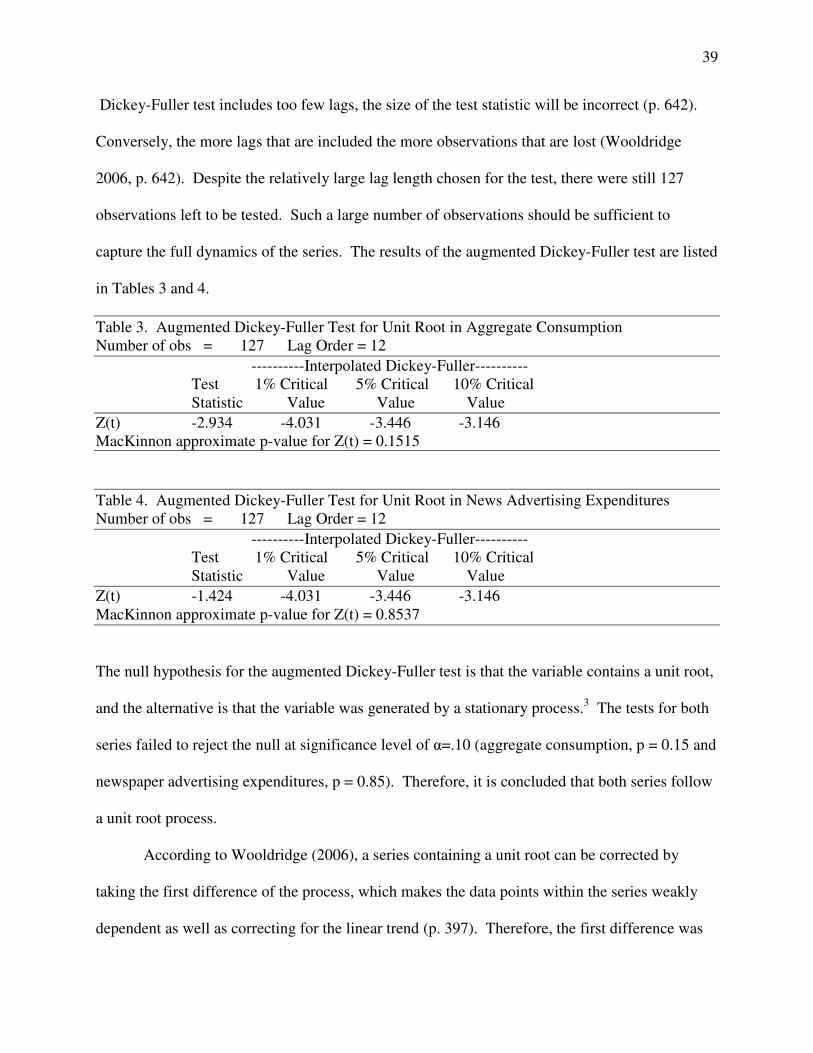
39

Dickey-Fuller test includes too few lags, the size of the test statistic will be incorrect (p. 642).

Conversely, the more lags that are included the more observations that are lost (Wooldridge

2006, p. 642). Despite the relatively large lag length chosen for the test, there were still 127

observations left to be tested. Such a large number of observations should be sufficient to

capture the full dynamics of the series. The results of the augmented Dickey-Fuller test are listed

in Tables 3 and 4.

Table 3. Augmented Dickey-Fuller Test for Unit Root in Aggregate Consumption Number of obs = 127 Lag Order = 12

----------Interpolated Dickey-Fuller---------- Test 1% Critical 5% Critical 10% Critical Statistic Value Value Value

Z(t) -2.934 -4.031 -3.446 -3.146 MacKinnon approximate p-value for Z(t) = 0.1515

Table 4. Augmented Dickey-Fuller Test for Unit Root in News Advertising Expenditures Number of obs = 127 Lag Order = 12



The null hypothesis for the augmented Dickey-Fuller test is that the variable contains a unit root,

and the alternative is that the variable was generated by a stationary process.3 The tests for both

series failed to reject the null at significance level of α=.10 (aggregate consumption, p = 0.15 and

newspaper advertising expenditures, p = 0.85). Therefore, it is concluded that both series follow

a unit root process.

According to Wooldridge (2006), a series containing a unit root can be corrected by

taking the first difference of the process, which makes the data points within the series weakly

dependent as well as correcting for the linear trend (p. 397). Therefore, the first difference was

40

taken for each time series to correct for the unit root process as well as the linear time trend. The

results for the augmented Dickey-Fuller test with the first difference of each series are listed in

Tables 5 and 6.

Table 5. Augmented Dickey-Fuller Test for Unit Root in the First Difference of Aggregate Consumption Number of obs = 127 Lag Order = 12



Table 6. Augmented Dickey-Fuller Test for Unit Root in the First Difference of News Advertising Expenditures Number of obs = 127 Lag Order = 12



Both tables show that taking the first difference allows the null to be rejected. Hence, the unit

root process within each series is corrected and inferences based upon the Classic Linear Model

should no longer be problematic.

Before the Granger causality test is conducted it is important to view the first difference

of aggregate consumption plotted against time, and then overlay the first difference of newspaper

advertising expenditures on the same graph. There is a lot of variation in the quarterly data over

the entire 140 observations, so the graphs were broken into roughly 35 observations each to

better capture the changes in aggregate consumption and newspaper advertising expenditures.

The results for the graphs are listed below:

41

Figure 3.1. Overlaid Graph of the Difference of the Log of Aggregate Consumption and the Difference of the Log of News Ad Expenditures Plotted Against Time; Observations 1 - 35

-.3

-.2

-.1

1971q3 1973q3 1975q3 1977q3 1979q3 Year

Aggregate

Consumption

News Ad

Expenditures

.1

.2

0

42


0

.1

.2

1979q3 1982q3 1985q3 1988q3

-.1

-.2

43


-.3

-.2

-.1

0

.1

.2

1989q1 1991q1 1993q1 1995q1 1997q1 Year

Aggregate

Consumption

News Ad

Expenditures

44


-.3

-.2

-.1

1997q3 1999q3 2001q3 2003q3 2005q3 Year

Aggregate

Consumption

News Ad

Expenditures

.2

.1

0

45

The dynamics of aggregate consumption and newspaper advertising expenditures become pretty

clear given the graphs. Quarterly changes in newspaper advertising expenditures are almost

identical to quarterly changes in aggregate consumption, but the variation in newspaper

advertising expenditures is much larger than the variation in aggregate consumption.

Changes in newspaper advertising expenditures appear to follow changes in aggregate

consumption, but it is difficult to determine by observation how long the lag may be. This

pattern appears to be consistent with Blank’s (1962) findings. To elucidate this point Figure 3.5

was constructed containing observations 70 – 80 (chosen as a convenience sample), to provide a

close up of the two overlaid series.

Figure 3.5. Overlaid Graph of the Difference of the Log of Aggregate Consumption and the Difference of the Log of News Ad Expenditures Plotted Against Time; Observations 70-80

-.2

-.1

0

.1

.2

1988q3 1989q1 1989q3 1990q1 1990q3 Year

Aggregate

Consumption

News Ad

Expenditures

46

The graphs appear to show that aggregate consumption is driving newspaper advertising

expenditures. It seems then that the graphs indicated support for the first hypothesis that

aggregate consumption Granger-causes national advertising expenditures. However, this is just

conjecture. The Granger causality test must be conducted to determine if aggregate consumption

is the driving force.

Results for the test of Granger causality are in Table 7. The first hypothesis predicted

that aggregate consumption Granger-caused national newspaper advertising expenditures.

Table 7. Granger Causality Testing Results

Number of Lags F-Statistic p-Value

H0: Ad Exp does 9 1.27 0.26 not cause 10 1.21 0.29 Agg Con 11 1.28 0.25 12 1.24 0.27 13 1.19 0.30 14 1.14 0.34 15 0.89 0.58 H0: Agg Con does 9 1.57 0.13 not cause 10 1.82 0.06* Ad Exp 11 1.71 0.08* 12 1.85 0.05** 13 1.90 0.04** 14 1.81 0.05** 15 1.73 0.06*

* p < .10, ** p < .05

The results from the Table 7 show that indeed aggregate consumption Granger-causes national

newspaper advertising expenditures, and not vice versa. Therefore, H1 is accepted—this finding

is also consistent in with the overlaid graphs.

The second hypothesis predicted that changes in aggregate consumption are not

proportional to changes in advertising expenditures. Tables 8.1 and 8.2 display the quarterly

percentage changes in national advertising expenditures and aggregate consumption.

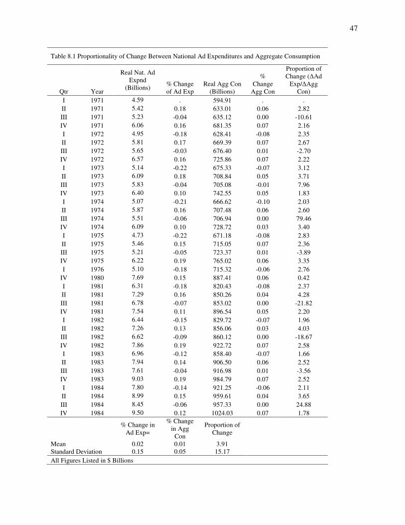
47

Table 8.1 Proportionality of Change Between National Ad Expenditures and Aggregate Consumption

Qtr Year

Real Nat. Ad Expnd

(Billions) % Change of Ad Exp

Real Agg Con (Billions)

% Change

Agg Con

Proportion of Change (∆Ad

Exp/∆Agg Con)

I 1971 4.59 . 594.91 . .

II 1971 5.42 0.18 633.01 0.06 2.82

III 1971 5.23 -0.04 635.12 0.00 -10.61

IV 1971 6.06 0.16 681.35 0.07 2.16

I 1972 4.95 -0.18 628.41 -0.08 2.35

II 1972 5.81 0.17 669.39 0.07 2.67

III 1972 5.65 -0.03 676.40 0.01 -2.70

IV 1972 6.57 0.16 725.86 0.07 2.22

I 1973 5.14 -0.22 675.33 -0.07 3.12

II 1973 6.09 0.18 708.84 0.05 3.71

III 1973 5.83 -0.04 705.08 -0.01 7.96

IV 1973 6.40 0.10 742.55 0.05 1.83

I 1974 5.07 -0.21 666.62 -0.10 2.03

II 1974 5.87 0.16 707.48 0.06 2.60

III 1974 5.51 -0.06 706.94 0.00 79.46

IV 1974 6.09 0.10 728.72 0.03 3.40

I 1975 4.73 -0.22 671.18 -0.08 2.83

II 1975 5.46 0.15 715.05 0.07 2.36

III 1975 5.21 -0.05 723.37 0.01 -3.89

IV 1975 6.22 0.19 765.02 0.06 3.35

I 1976 5.10 -0.18 715.32 -0.06 2.76

IV 1980 7.69 0.15 887.41 0.06 0.42

I 1981 6.31 -0.18 820.43 -0.08 2.37

II 1981 7.29 0.16 850.26 0.04 4.28

III 1981 6.78 -0.07 853.02 0.00 -21.82

IV 1981 7.54 0.11 896.54 0.05 2.20

I 1982 6.44 -0.15 829.72 -0.07 1.96

II 1982 7.26 0.13 856.06 0.03 4.03

III 1982 6.62 -0.09 860.12 0.00 -18.67

IV 1982 7.86 0.19 922.72 0.07 2.58

I 1983 6.96 -0.12 858.40 -0.07 1.66

II 1983 7.94 0.14 906.50 0.06 2.52

III 1983 7.61 -0.04 916.98 0.01 -3.56

IV 1983 9.03 0.19 984.79 0.07 2.52

I 1984 7.80 -0.14 921.25 -0.06 2.11

II 1984 8.99 0.15 959.61 0.04 3.65

III 1984 8.45 -0.06 957.33 0.00 24.88

IV 1984 9.50 0.12 1024.03 0.07 1.78

% Change in

Ad Exp=

% Change in Agg

Con

Proportion of Change

Mean 0.02 0.01 3.91 Standard Deviation 0.15 0.05 15.17

All Figures Listed in $ Billions

48

Table 8.2 Proportionality of Change Between National Ad Expenditures and Aggregate Consumption

Qtr Year

Real Nat. Ad

Expnd (Billion)

% Change of Ad Exp

Real Agg Con (Billions)

% Change

Agg Con

Proportion of Change (∆Ad

Exp/∆Agg Con)

IV 1990 10.61 . 1242.35 . .

I 1991 8.03 -0.24 1141.57 -0.08 2.99

II 1991 9.11 0.13 1189.09 0.04 3.23

III 1991 8.73 -0.04 1196.99 0.01 -6.31

IV 1991 10.04 0.15 1249.64 0.04 3.41

I 1992 7.75 -0.23 1175.90 -0.06 3.87

II 1992 8.98 0.16 1220.92 0.04 4.17

III 1992 8.62 -0.04 1233.12 0.01 -4.04

IV 1992 10.09 0.17 1303.73 0.06 2.98

I 1993 7.94 -0.21 1208.62 -0.07 2.93

II 1993 8.98 0.13 1264.51 0.05 2.84

III 1993 8.73 -0.03 1277.35 0.01 -2.79

IV 1993 10.39 0.19 1348.21 0.06 3.44

I 1994 8.24 -0.21 1260.56 -0.07 3.18

II 1994 9.33 0.13 1310.51 0.04 3.32

III 1994 9.24 -0.01 1321.75 0.01 -1.05

IV 1994 10.95 0.19 1396.45 0.06 3.28

I 1995 8.65 -0.21 1290.63 -0.08 2.77

II 1995 9.64 0.11 1351.03 0.05 2.44

III 1995 9.38 -0.03 1360.77 0.01 -3.76

IV 1995 11.50 0.23 1429.95 0.05 4.45

IV 2000 13.84 -0.20 1759.51 -0.04 0.22

I 2001 10.18 -0.26 1665.09 -0.05 4.92

II 2001 10.84 0.06 1718.62 0.03 2.01

III 2001 10.31 -0.05 1717.75 0.00 96.03

IV 2001 11.90 0.15 1808.23 0.05 2.92

I 2002 9.38 -0.21 1713.79 -0.05 4.06

II 2002 10.47 0.12 1766.21 0.03 3.82

III 2002 10.25 -0.02 1775.02 0.00 -4.29

IV 2002 12.21 0.19 1843.23 0.04 4.99

I 2003 9.34 -0.23 1750.06 -0.05 4.65

II 2003 10.43 0.12 1814.42 0.04 3.15

III 2003 10.18 -0.02 1829.27 0.01 -2.85

IV 2003 12.26 0.20 1900.75 0.04 5.22

I 2004 9.45 -0.23 1829.91 -0.04 6.15

II 2004 10.54 0.12 1883.59 0.03 3.94

III 2004 10.27 -0.03 1892.18 0.00 -5.63

IV 2004 12.39 0.21 1970.02 0.04 5.01

% Change in

Ad Exp=

% Change in Agg

Con

Proportion of Change

Mean 0.02 0.01 3.91 Standard Deviation 0.15 0.05 15.17

All figures listed in $ Billions

49

The furthest column to the right labeled “Proportion of Change” is the quotient of the quarterly

percentage change in advertising expenditures and the quarterly percentage change in aggregate

consumption. The table clearly shows that no stable proportional changes occurred during the

140 observation period, nor are there any trends in the proportionality. Therefore, H2 is

supported; a change in one of the variables is not accompanied by a proportional change in the

other variable.

The third hypothesis predicts that advertising expenditures lag behind aggregate

consumption. This hypothesis can be tested by observing the overlaid graphs in Figures 3.1-3.5.

One may argue that Tables 2.1 and 2.2, which list quarterly statistics for these variables and their

respective changes, could be used to test H3. However, both national advertising expenditures

and aggregate consumption contain a linear trend and strong persistence (unit root process) as

established by the Augmented Dickey-Fuller tests (Tables 3-4). Therefore, the first differences

were taken for both variables to eliminate the strong persistence. As demonstrated in Tables 5

and 6, the persistence was removed from both variables once the first differences were taken.

The overlaid graphs with first differences seem to clearly show that changes in

advertising consumption lag behind changes in aggregate consumption. However, to clarify the

relationship Tables 9.1 through 9.4 were constructed to demonstrate the first differences of the

series in $ billion increments.

Comparing these tables to the periods of contraction in the economy listed by NBER

(n.d.)— (1) Q4, 1973 to Q1, 1975, (2) Q1, 1980 to Q3, 1980, (3) Q2, 1981 to Q4, 1982, (4) Q3,

1990 to Q1, 1991, and (5) Q1, 2001 to Q4, 2001—we see markedly different results from the

descriptive statistics within Tables 2.1-2.4. For example, in the first contraction outlined by the

NBER the newspaper industry experienced approximately a $76 billion (Q1, 1974) and $58

50

Table 9.1. The First Differences in Aggregate Consumption and Advertising Expenditures

qtr Year Difference in Agg Con Difference in Ad Exp

I 1971 . .

II 1971 0.83 38.10

III 1971 -0.19 2.11

IV 1971 0.83 46.23

I 1972 -1.11 -52.94

II 1972 0.86 40.98

III 1972 -0.16 7.01

IV 1972 0.92 49.46

I 1973 -1.43 -50.53

II 1973 0.95 33.51

III 1973 -0.26 -3.76

IV 1973 0.57 37.47

I 1974 -1.33 -75.93

II 1974 0.80 40.86

III 1974 -0.36 -0.54

IV 1974 0.58 21.78

I 1975 -1.36 -57.54

II 1975 0.73 43.87

III 1975 -0.25 8.32

IV 1975 1.01 41.65

I 1976 -1.12 -49.70

II 1976 0.91 38.83

III 1976 -0.14 2.81

IV 1976 1.04 50.47

I 1977 -1.63 -59.43

II 1977 1.01 34.71

III 1977 -0.10 7.01

IV 1977 1.15 51.98

I 1978 -1.67 -64.41

II 1978 1.16 43.98

III 1978 -0.34 5.36

IV 1978 1.15 48.39

I 1979 -1.66 -61.49

II 1979 1.00 23.51

III 1979 0.08 2.41

IV 1979 0.83 51.05

Agg Con Ad Expend

Mean 0.09 8.45

Standard Deviation 0.97 41.14

All figures based upon $ Billions

51



I 1980 -1.68 -66.35

II 1980 0.54 2.37

III 1980 -0.09 7.07

IV 1980 1.03 53.82

I 1981 -1.38 -66.98

II 1981 0.98 29.83

III 1981 -0.51 2.76

IV 1981 0.76 43.52

I 1982 -1.10 -66.82

II 1982 0.82 26.34

III 1982 -0.64 4.06

IV 1982 1.24 62.60

I 1983 -0.90 -64.32

II 1983 0.98 48.10

III 1983 -0.33 10.48

IV 1983 1.42 67.81

I 1984 -1.23 -63.54

II 1984 1.19 38.36

III 1984 -0.54 -2.28

IV 1984 1.05 66.70

I 1985 -1.16 -63.78

II 1985 0.79 46.29

III 1985 -0.42 11.57

IV 1985 1.20 59.88

I 1986 -1.44 -75.77

II 1986 1.23 43.82

III 1986 -0.51 14.31

IV 1986 1.30 58.97

I 1987 -1.38 -90.66

II 1987 1.28 58.95

III 1987 -0.54 8.23

IV 1987 0.96 60.17

I 1988 -1.33 -74.86

II 1988 1.12 43.79

III 1988 -0.59 8.42

IV 1988 1.09 72.17

I 1989 -1.67 -92.73

II 1989 1.13 44.66

III 1989 -0.64 11.56

IV 1989 1.35 65.09

Agg Con Ad Expend

Mean 0.08 8.59



52



I 1990 -2.21 -90.44

II 1990 1.15 45.24

III 1990 -0.55 4.54

IV 1990 0.95 48.90

I 1991 -2.58 -100.78

II 1991 1.08 47.52

III 1991 -0.38 7.90

IV 1991 1.31 52.65

I 1992 -2.29 -73.74

II 1992 1.23 45.02

III 1992 -0.36 12.20

IV 1992 1.47 70.61

I 1993 -2.15 -95.11

II 1993 1.04 55.89

III 1993 -0.25 12.84

IV 1993 1.66 70.86

I 1994 -2.15 -87.65

II 1994 1.09 49.95

III 1994 -0.09 11.24

IV 1994 1.71 74.70

I 1995 -2.30 -105.82

II 1995 0.99 60.40

III 1995 -0.26 9.74

IV 1995 2.12 69.18

I 1996 -2.60 -87.53

II 1996 1.00 54.44

III 1996 0.03 7.03

IV 1996 1.89 71.22

I 1997 -2.34 -83.90

II 1997 1.12 48.54

III 1997 0.03 23.42

IV 1997 1.96 73.84

I 1998 -2.48 -89.88

II 1998 1.13 75.98

III 1998 -0.13 14.02

IV 1998 1.96 80.61

I 1999 -2.55 -90.54

II 1999 1.09 74.13

III 1999 -0.06 13.41

IV 1999 2.05 79.12

Agg Con Ad Expend

Mean 0.06 11.49



53



I 2000 -2.71 -73.05

II 2000 1.25 55.13

III 2000 -0.36 6.24

IV 2000 2.06 77.33

I 2001 -3.66 -94.42

II 2001 0.66 53.53

III 2001 -0.53 -0.87

IV 2001 1.59 90.48

I 2002 -2.52 -94.44

II 2002 1.09 52.42

III 2002 -0.22 8.81

IV 2002 1.96 68.21

I 2003 -2.87 -93.17

II 2003 1.09 64.36

III 2003 -0.25 14.85

IV 2003 2.08 71.48

I 2004 -2.81 -70.84

II 2004 1.09 53.68

III 2004 -0.27 8.59

IV 2004 2.12 77.84

I 2005 -3.00 -87.03

II 2005 1.06 65.99

III 2005 -0.33 19.57

IV 2005 1.94 70.02

Agg Con Ad Expend

Mean -0.06 14.36



54

billion (Q1, 1975) slowdown in advertising expenditures. Newspaper advertising expenditures

also experienced large slowdowns (each in excess of $66 billion) during the third contraction

listed by the NBER. One of the largest slowdowns in newspaper ad expenditures correspond

with the fourth contraction period in Q1, 1991 with a downturn in advertising expenditures in

excess of $100 billion.

Beyond the descriptive statistics within Tables 9.1-9.4 there is one very important

observation. Newspaper advertising expenditures do not lag behind aggregate consumption as

predicted by H3. Instead the contractions occurred almost without fail within the same quarter.

However, most downturns within newspaper ad expenditures followed the seasonal trend

observed earlier, with contractions in the first quarter of each year when newspaper advertising

slows in the winter months after a busy holiday shopping season. In fact, during the observation

period only three downturns in ad spending did not occur in Q1—(1) Q3, 1974, (2) Q3, 1984, (3)

Q3, 2001. None of those observations lagged behind a contraction in aggregate consumption,

instead each occurred in the same quarter that aggregate consumption contracted. Therefore, H3

is rejected.

55

CHAPTER 5

CONCLUSION

The first hypothesis predicted that aggregate consumption Granger- causes national newspaper

advertising expenditures. National newspaper advertising expenditures represent a sizeable

percentage of total advertising spending. The Granger causality test supported the hypothesis

between ten and fifteen lag lengths. These results are consistent with the findings of Ashley et

al. (1980) that aggregate consumption Granger-causes advertising expenditures but not the other

way around. However, these results are not consistent with Jung and Seldon (1995) who found

bi-directional Granger causality between aggregate consumption and newspaper advertising

expenditures. The disagreement with Jung and Seldon (1995) perhaps stems from their use of

annual advertising data. Clarke (1970) found a strong tendency toward bias in annual data

intervals. The results of the current study’s Granger causality also seem consistent with a large

majority of organizations allocating money to their advertising budget by utilizing the

percentage-of-sales method (Patti & Blasko, 1981, p.25). The results are also consistent with the

findings of White and Miles (1996) that a majority of organizations follow the US tax code,

which treats advertising expenditures as single period business expenses, with the cost of the

current year’s advertising campaign being deducted from the year’s gross income (pp. 43-44). If

this is the case, it would seem intuitive that aggregate consumption is driving advertising

spending as organization’s budgets react to changes in sales levels. If sales levels are affected by

business cycles then it would make sense that advertising spending would follow those cycles

when a percentage-of-sales budget method is used. In other words, it seems that aggregate

consumption is driving sales, and sales are driving advertising budgets. Therefore, changes in

aggregate consumption lead to changes in advertising expenditures.

56

The second hypothesis predicted changes in aggregate consumption would not be

proportionate to changes in newspaper advertising expenditures. This hypothesis followed from

the findings of Picard (2001) and Chang and Chan-Olmstead (2005), who each identified that

disproportionate changes in cross nation studies. In conjunction, this study revealed that the

changes were very disproportionate from 1971-2005 using 140 observations. Such findings cast

a slight shadow on the belief that there is a causal connection between aggregate consumption

and newspaper ad expenditures. A strong causal connection could be expected to produce a

more stable, proportionate, change throughout the series. This disproportionality leads to the

belief that there may be other intervening variables affecting changes to aggregate consumption

and newspaper ad expenditures. Newspaper advertising is highly dependent on local market

conditions because significant proportions of advertising revenue come from the sale of

classified and local display advertising. There could also be environmental factors, such as the

decay of advertising growth within the newspaper industry over the past couple of decades.

The third hypothesis predicted that newspaper advertising expenditures would lag behind

business cycles. This prediction was based on the belief that aggregate consumption will drive

ad spending if a large majority of organizations use the percentage-of-sales budget allocation

method. Blank (1962) had found that expenditures lagged behind business cycles by about one

quarter.

Figures 3.1 through 3.5 seemed to show that ad spending lagged aggregate consumption.

However, the analysis within Tables 9.1 through 9.4 revealed that changes in business cycles and

changes in advertising spending almost always occurred concurrently. There is a possibility that

ad spending is lagging behind aggregate consumption, but that the data intervals need to be

shorter to observe the lags. For example, perhaps monthly observations would indicate a lag.

57

However, if a majority of businesses use the percentage-of-sales method and sales respond to

changes in business cycles, one month is probably not sufficient time for the advertising budget

to feel any effects from a turn in a business cycle. Thus, the rejection of the third hypothesis

casts a larger shadow on a causal relation between aggregate consumption and national

advertising expenditures.

Despite strong evidence in the Granger causality test that aggregate consumption predicts

newspaper ad spending, the combination of the last two hypothesises raise significant doubt that

a true causal relationship exists. Perhaps the best interpretation of the relationship is to use

Sørenson’s (2005) definition, that Granger causality simply means aggregate consumption is a

good linear predictor for newspaper advertising expenditures. These findings support the need

for the academic community to continue building models to explain how advertising affects the

economy. There is a particular need for a macro-economic model of the economics of

advertising. There is a strong possibility that several intervening variables affect the

relationship, such as environmental factors, and controlling for these variables could better the

capture dynamics between ad spending and aggregate consumption. For example, a vector

autoregression model controlling for the observed seasonal trends and various other

environmental factors may reveal more about the relationship than was observed here. Such a

model was unfortunately beyond the scope of this study.

Several limitations were encountered in this study. First, the quarterly data were limited

to newspaper advertising expenditures. Second, this data was supplied by the Newspaper

Association of America and comes from a private research firm which does not disclose its

methods. Therefore, the expenditure estimates could contain potential flaws. Third, the

interpretation of the Granger causality test was limited to linear prediction and does not denote a

58

deeper philosophical meaning of causality. Fourth, it should be duly noted that a significant

percentage of newspaper advertising expenditures are composed of retail sales, and a significant

portion of the retail advertising sales is local in orientation. Finally, it is generally accepted that

the principle of relative constancy, referred to in Chang and Chan-Olmstead (2005), has been

dismissed; it was mentioned in this study to explain the motivation for Chang and Chan-

Olmstead’s (2005) research.

Further research should investigate a fully-specified macroeconomic model of the

dynamics between aggregate consumption and newspaper advertising expenditures. However,

there needs first to be more understanding of the macroeconomic effects of advertising to

develop a fully-specified model. As discovered in the literature review, there is an ample

discussion of the microeconomic effects with little to no discussion of macroeconomic effects.

Organizations can benefit from the findings of this study since aggregate consumption

serves as a good predictor for advertising expenditures. Perhaps current aggregate consumption

data can be used in budget forecasts. In other words, aggregate consumption figures can be used

in an organization’s marginal analysis to predict when incremental revenues may change and

improve forecasting of advertising expenditures.

According Coen (2005), total national advertising revenues have remained stable at more

than 2 percent of total GDP since 1990 (p. 6). Thus, it is hard to believe that advertising has no

effect in the economy. Such observations raise substantial heuristic questions about the nature of

the relationship between GDP and advertising. This study has brought the academic community

even closer to elucidating this very complicated relationship.

59

REFERENCES

Aaker, D.A., & Myers, J.G. (1987). Advertising Management (3rd ed.). Englewood Cliffs, New

Jersey: Prentice-Hall, Inc.

Ackerberg, D.A. (2003). Advertising, learning, and consumer choice in experience good

markets: An empirical examination. International Economic Review, 44(3), 1007-1040

Ashley, R., Granger, C.W.J., & Schmalensee, R. (1980). Advertising and aggregate

consumption: An Analysis of Causality. Econometrica, 48(5), 1149-1168.

Berndt, E.R. (1996). The Practice of Econometrics: Classic and Contemporary. Reading:

Addison-Wesley Pub., Co.

Blank, D. M. (1962). Cyclical behavior of national advertising. The Journal of Business, 35(1),

14-27.

Borden, N. H. (1942). The Economic Effects of Advertising. Chicago: Irwin, In.

Bureau of Economic Analysis’ National Economics Accounts. (n.d.) (2007). Retrieved January

23, 2007 from

http://www.bea.gov/national/nipaweb/TableView.asp?SelectedTable=65&FirstYear=200

4&LastYear=2006&Freq=Qtr

Chamberlin, E. H. (1933). The Theory of Monopolistic Competition: A Re-orientation of the

Theory of Value. Cambridge: Harvard University Press.

Chan-Olmstead, S.M., & Chang, B.-H. (2005). Relative constancy of advertising spending: A

cross-national examination of advertising expenditures and their determinants. The

International Journal for Communication Studies, 67(4), 339-357.

Clarke, D.G. (1976). Econometric measurement of the duration of advertising effect on sales.

Journal of Marketing Research 8, 345-357.

60

Coen, R. (2005). Insider’s Report. Retrieved March 21, 2007, from

http://www.universalmccann.com/pdf/Insiders1205.pdf

Coen, R. (2006). [Estimates of national advertising expenditures]. Unpublished raw data.

Comanor, W.S., & Wilson, T.A. (1967). Advertising market structure and performance. The

Review of Economics and Statistics, 49(4), 423-440.

Dhala, N. K. (1978). Assessing the long-term value of advertising. Harvard Business Review, 56

(1), 87-95.

Ekelund, R. B., & Gramm, W.P. (1969). A reconsideration of advertising expenditures,

aggregate demand, and economic stabilization. Quarterly Review of Economics and

Business, 9, 71-77.

Ekelund, R. B., & Saurman, D. S. (1998). Advertising and the Market Process. San Francisco:

Pacific Research Institute for Public Policy

Farris, P.W., & Albion, M.S. (1980). The impact of advertising on the price of consumer

products. Journal of Marketing, 44, 17-35.

Galbraith, J.K. (1958). The Affluent Society. Boston: Houghton Mifflin Co.

Greene, W.H. (2003). Econometric Analysis (5th

ed.). New York: Pearson Education

International.

Hansen, A. H. (1960). Economic Issues of the 1960’s. New York: McGraw-Hill.

Jung, C. & Seldon, B. (1995). The macroeconomic relationship between advertising and

consumption. Southern Economic Journal, 61(3), 577-587.

61

Low, G.S., & Mohr, J.J. (1999). Setting advertising and promotion budgets in multi-brand

companies. Journal of Advertising Research, 39 (1), 67-78.

Kaldor, N. The economic aspects of advertising. The Review of Economic Studies, 18(1), 1-27.

Kessides, I. N. (1986). Advertising, sunk costs, and barriers to entry. Review of Economics and

Statistics, 68, 84-95.

Leffler, K. B. (1981). Persuasion or information? The economics of prescription drug

advertising. Journal of Law and Economics, 24(1), 45-74.

Marshall, A. (1920). Principles of Economics. London: Macmillan and Co.

Marshall, A. (1919). Industry and Trade. London: Macmillan and Co.

Mitra, A. (1995). Advertising and the stability of consideration sets over multiple purchase

occasions. International Journal in Marketing, 12, 81-94.

Newspaper Association of America. (2006). Quarterly Newspaper Advertising Expenditures.

Retrieved January 23, 2007, from http://www.naa.org/trends-and-numbers/market-

databank/quarterly-newspaper-advertising-expenditures.aspx

National Bureau of Economic Research (n.d.). US Business Cycle Expansions and Contractions.

Retrieved March 12, 2007, from http://www.nber.org/cycles.html.

Ott, R.L. & Longnecker, M. (2001). An Introduction to Statistical Methods and Data Analysis

(5th ed.). New York: Thomson Learning, Inc.

Patti, C.H., & Blasko, V. (1981). Budgeting practices of big advertisers. Journal of Advertising

Research, 21(6), 23-29

62

Picard, R. (2001). Effects of recessions on advertising expenditures: An exploratory study of

economic downturns in nine developed nations. The Journal of Media Economics, 14(1),

1-14.

Robinson, J. (1936). The Economics of Imperfect Competition. London: Macmillan and Co.

Schmalensee, R. (1982). Product differentiation advantages of pioneering brands. American

Economic Review, 72, 349-365.

Sørenson, B.E. (2005). Granger causality. Unpublished manuscript, University of Houston,

Texas. Available at http://www.uh.edu/~bsorense/gra_caus.pdf.

Stigler, G. (1960). Monopoly and oligopoly by merger. American Economic Review, 50, 27.

Stigler, G (1968). The Organization of Industry. Homewood, Illinois: Richard D. Irwin, Inc.

Verdon, W.A., McConnell, C.R., & Roesler, T.W. (1968). Advertising expenditures as an

economic stabilizer. Quarterly Review of Economics and Business, 8, 7-18.

White, J.B., & Miles, P.M. (1996). The financial implications of advertising as an investment.

Journal of Advertising Research, 36, 43-52.

Wynne, M. A. (2000). Measuring and detecting inflation. Dallas, TX: Federal Reserve Bank of

Dallas. Retrieved on March 12, 2007, from

http://www.dallasfed.org/research/indepth/2000/id0004.pdf

Yang, C. Y. (1964). Variations in the cyclical behavior of advertising. Journal of Marketing,

28, 25-30.

63

FOOTNOTES

1. Schmalensee (1982) defines an experience good as existing when “the only way a

consumer can resolve uncertainty about quality is purchase a brand and try it. One trial is both

necessary and sufficient to determine whether or not any single brand works” (p. 350).

2. It is arguable whether the consumer price index (CPI) price deflator supplied by the

Bureau of Labor Statistics or the personal consumption expenditure (PCE) price deflator

supplied by the Bureau of Economics Analysis represents a better deflator for empirical analysis.

The indices are chosen based upon which offers the best measure of inflation. Ultimately the

PCE index was chosen based upon a presentation by Wynne (2000) in which he stated that, “the

PCE is probably the most accurate of the government’s inflation measures… [and it] is the

preferred inflation measure of [former] Chairman Greenspan” (p. 3). The two measures differ

because the CPI only represents prices paid by urban consumers, and the PCE represents prices

paid by all consumers, urban and rural (Wynne, 2000, p. 5). Wynne (2000) argues that the main

difference, however, is that the PCE deflator accounts for shifting spending patterns whereas the

CPI deflator relies on spending patterns from several years ago (p. 5). He argues that goods

which actually become cheaper over time will tend to be underrepresented in the aggregate CPI

numbers, causing inflation to be overstated (Wynne, 2000, p. 5). Therefore, this researcher

decided to utilize the PCE deflator to offer a truer estimation of inflation in the United States.

3. Wooldridge (2006) defines a stationary process as, “a time series process where the

marginal and all joint distributions are invariant across time” (p. 870).

Documents

EFFECTS OF NATIONAL NEWSPAPER ADVERTISING …