University of Wisconsin MilwaukeeUWM Digital Commons

Theses and Dissertations

August 2013

Effects of Internal Resistance on Performance ofBatteries for Electric VehiclesRohit Anil UgleUniversity of Wisconsin-Milwaukee

Follow this and additional works at: https://dc.uwm.edu/etdPart of the Mechanical Engineering Commons

This Thesis is brought to you for free and open access by UWM Digital Commons. It has been accepted for inclusion in Theses and Dissertations by anauthorized administrator of UWM Digital Commons. For more information, please contact open-access@uwm.edu.

Recommended CitationUgle, Rohit Anil, "Effects of Internal Resistance on Performance of Batteries for Electric Vehicles" (2013). Theses and Dissertations. 241.https://dc.uwm.edu/etd/241

EFFECTS OF INTERNAL RESISTANCE ON

PERFORMANCE OF BATTERIES FOR ELECTRIC

VEHICLES

by

Rohit A Ugle

A Thesis Submitted in

Partial Fulfillment of the

Requirements for the Degree of

Master of Science

in Engineering

at

The University of Wisconsin-Milwaukee

August 2013

ii

ABSTRACT

EFFECTS OF INTERNAL RESISTANCE ON PERFORMANCE OF BATTERIES FOR ELECTRIC

VEHICLES

by

Rohit A Ugle

The University of Wisconsin-Milwaukee, 2013 Under the Supervision of Professor Anoop K. Dhingra

An ever increasing acceptance of electric vehicles as passenger cars relies on better

operation and control of large battery packs. The individual cells in large battery packs do

not have identical characteristics and may degrade differently due to their manufacturing

variability and other factors. It is beneficial to evaluate the performance gain by replacing

certain battery modules/cells during actual driving.

The following are the objectives of our research. We will develop an on-line battery

module degradation diagnostic scheme using the intrinsic signals of a battery pack

equalization circuit. Therefore, a battery “health map” can be constructed and updated in

real time. Next based on the derived battery health map, the performance of the battery

pack will be evaluated a user specified trip so as to evaluate the “worthiness of replacing”

certain modules/cells.

Different electric vehicles have different performance for the same driving cycle. These

variations are due to variation in driving patterns, traffic, different light patterns, random

iii

behavior of the drivers etc. To account for this random behavior of the electric vehicle

performance we generate 100 random trip cycles. We aim to model the behavior of the

driving cycle and battery behavior.

Finally, the thesis also explores the possibility of energy exchange between the battery

packs and the smart grid. In the smart grid scenario where we have the knowledge of the

electricity price and the load patterns on the grid, it is beneficial for the user to schedule

charging and discharging patterns for electric vehicles. Our research will define charging

and discharging patterns throughout the life of the battery. We will optimize the charging

and discharging times and define the opportunity cost for each day during summer and

winter months. The objective is to maximize the profit earned by selling excess energy in

the battery to the grid and minimize the charging cost for the electric vehicle.

iv

Dedicated to my wife Mithila and my Parents who always motivated and supported me to

continue my education

v

TABLE OF CONTENTS

1. Introduction ...................................................................................................................1

1.1 Hybrid and Plug-in Hybrid Electric Vehicles .........................................................4

1.1.1 Parallel Hybrid Vehicle ...................................................................................5

1.1.2 Series Hybrid Vehicle .....................................................................................5

1.1.3 Power-Split Hybrid Vehicle ............................................................................6

2. Literature Review ..........................................................................................................9

2.1 Electric Vehicle Model ...........................................................................................9

2.1.1 Aerodynamic Force .........................................................................................9

2.1.2 Rolling Resistance...........................................................................................10

2.1.3 Acceleration Force ..........................................................................................10

2.1.4 Wheel Torque ..................................................................................................10

2.1.5 Motor Torque ..................................................................................................11

2.2 Electric Motor Model ..............................................................................................11

2.3 Electric Vehicle Battery ..........................................................................................13

2.3.1 Lithium ion Batteries .......................................................................................16

2.3.2 Battery Modeling Technique ..........................................................................17

2.3.3 Battery Equivalent Circuit Representation .....................................................18

2.3.4 Battery Equalization ........................................................................................22

2.4 Smart Grid ...............................................................................................................24

3. Simulation Results for Equalization ............................................................................26

3.1 Electric Vehicle and Motor .....................................................................................26

3.2 Battery Equivalent Circuit ......................................................................................27

vi

3.3 Battery State of Charge Calibration ........................................................................28

3.4 Battery Equalization Scheme ..................................................................................31

3.5 Worthiness of Replacement ....................................................................................36

3.6 Driving Cycle ..........................................................................................................37

3.7 Two Module Battery Pack ......................................................................................39

3.8 Three Module Battery Pack ....................................................................................43

4. Simulation Results for Group Performance ................................................................49

4.1 Driving Cycle ..........................................................................................................49

4.2 Electricity Cost........................................................................................................51

4.3 Battery Charging Configuration .............................................................................59

4.4 Battery Discharging Configuration .........................................................................62

4.5 Optimizing Trip Cost ..............................................................................................66

4.6 Opportunity Cost .....................................................................................................67

4.7 Optimized Battery Cycles .......................................................................................68

5. Conclusion and Recommendations ..............................................................................83

6. References .......................................................................................................................85

vii

LIST OF FIGURES

Fig. 1.1. Energy Information............................................................................................... 2

Fig. 1.2. Smart Grid Architecture ....................................................................................... 3

Fig. 1.3. Parallel Hybrid Architecture ................................................................................. 5

Fig. 1.4. Architecture of a series hybrid vehicle ................................................................. 5

Fig. 1.5. Architecture of power-split hybrid ....................................................................... 6

Fig. 2.1. Typical initial Lithium ion battery pack ............................................................. 17

Fig. 2.2. (a) Thevenin electrical model (b) Impedance based electrical model ................ 19

Fig. 2.3. Runtime Based Electrical Battery Models.......................................................... 20

Fig. 2.4. Non-Linear RC battery proposed for estimation of SOC ................................... 21

Fig. 2.5. Remapped battery model .................................................................................... 22

Fig. 2.6.Multi-winding transformer (a) Conventional Approach (b) Modularized

Approach .............................................................................................................23

Fig. 3.1. Battery equivalent circuit model......................................................................... 28

Fig. 3.2. Battery Equalization Circuit ............................................................................... 32

Fig. 3.3. Typical switching waveform of the battery equalizer when VB1 >VB2. .............. 33

Fig. 3.4. Route map of the sample trip .............................................................................. 37

Fig. 3.5. (a) Motor speed during driving, (b) Motor torque profile during driving .......... 38

Fig. 3.6. Battery module SOC trajectories for with Case #1with the example driving

cycle ....................................................................................................................40

Fig. 3.7. Two Module Battery SOC for example driving cycle for Case-2 ...................... 41

Fig. 3.8. SOC trajectory for case1 of three-module battery pack ..................................... 44

Fig. 3.9. Battery SOC trajectories for three modules for Case 2 of Table 6 ..................... 45

viii

Fig. 3.10. Battery SOC trajectories for three modules for Case 2 for intermediate

equalization ................................................................................................... 47

Fig. 4.1. Inputs for driving cycle, (a) Acceleration for 100 vehicles for total distance

(b) Velocity for 100 vehicles for total distance ..................................................50

Fig. 4.2. Average energy requirement and cost for a week in summer, (a) Average

energy cost for a week in summer, (b) Average energy requirement for a

week in summer ..................................................................................................52

Fig. 4.3. Daily energy requirement and cost on daily basis for a week in summer, (a)

Energy price per hour on daily basis for a week in summer, (b) Energy

requirement for a week on daily basis in summer ..............................................54

Fig. 4.4. Average energy requirement and cost for a week in winter, (a) Average

energy cost for a week in winter, (b) Average energy requirement for a

week in winter .....................................................................................................56

Fig. 4.5. (a) Energy price per hour on daily basis for a week in summer, (b)

Energy requirement for a week on daily basis in winter ....................................57

Fig. 4.6. Charging time for batteries in all the groups ...................................................... 60

Fig. 4.7. Battery performances, (a) Battery performance of group 1 batteries, (b)

Battery performance of group 2 batteries, (c) Battery performance of

group 3 batteries, (d) Battery performance of group 4 batteries .........................64

Fig. 4.8. Batteries performance connected to grid ............................................................ 69

Fig. 4.9. Number of batteries connected to grid ............................................................... 70

ix

Fig. 4.10. Performance of batteries during a week in summer, (a) Monday cycle,

(b) Tuesday cycle, (c) Wednesday cycle, (d) Thursday cycle, (e) Friday

cycle ...................................................................................................................73

Fig. 4.11. The average performance of batteries in summer ............................................ 75

Fig. 4.12. Performance of batteries during a week in winter, (a) Monday cycle, (b)

Tuesday cycle, (c) Wednesday cycle, (d) Thursday cycle, (e) Friday

Cycle ...................................................................................................................80

Fig. 4.13. Costs incurred and gained during charging and exchanging energy with

grid in winter .......................................................................................................82

x

LIST OF TABLES

Table 2.1.Typical permanent magnet electric motor configurations ................................ 13

Table 2.2. Commercially available batteries..................................................................... 15

Table 2.3. Comparison for Lithium Ion and lead acid batteries ....................................... 16

Table 3.1. Configuration of Electric vehicle. .................................................................... 27

Table 3.2. Initial Conditions of Two Module Simulation Study ...................................... 39

Table 3.3. Initial conditions of individual battery modules for simulation study ............. 43

Table 4.1. Battery internal resistance as per the age of battery during discharging ......... 59

Table 4.2. Battery energy capacity available for exchange .............................................. 68

Table 4.3. Cost of battery cycle per day in summer ......................................................... 74

Table 4.4. Opportunity cost for Week in summer ............................................................ 76

Table 4.5. Cost of battery cycle per day in winter ............................................................ 81

Table 4.6. Opportunity Cost for a week in winter ............................................................ 83

xi

ACKNOWLEDGMENTS

I would take this opportunity to thank my advisor, Professor Anoop Dhingra for

his continuous support, guidance, patience and advice throughout my thesis work. I

appreciate my thesis committee members: Dr Ron Perez and Dr Wilkistar Otieno for their

support and suggestions. Also, I would like to thank Professor Yaoyu Li for his help in

my research.

I would like to thank all my friends in the Design Optimization group. I thank my

parents for all their effort to develop me as a person.

Last, but not the least, special thanks to my dear wife, Mithila. Without her

support and patience, this work would not have been possible.

1

1. Introduction

An ever increasing need for better and efficient transportation has motivated the

automobile industry to look for alternative sources of energy in lieu of conventional

energy sources. The electric vehicles are clean i.e. they have lower CO2, CO and

hydrocarbon emissions than the conventional energy resources. The vehicles which use

non-conventional energy sources are multi sourced vehicles which use petroleum-battery,

diesel-battery or fuel cell-battery etc. The battery forms a critical element for driving non-

conventional vehicles. Electric vehicles (EV) require large battery packs with high energy

and power densities to become a competitive choice of transport. These batteries have

many cells/modules in series and parallel. Acceptance of these vehicles results from

better operation and control of large battery packs.

Recently, addressing the problems of green house effect, clean energy requirements and

the need for renewable energy resources, electric vehicles have gained ground [1].

Today’s research in electric vehicle design and battery technology is a major challenge.

The automobile industry is due for a major overhaul to achieve minimum pollution,

overcome the problem of limited availability of conventional energy resources, and

minimize the cost of travelling [2].

There is a continuous increase in the need of energy around the globe. The sources of

energy have been changing drastically in the last decades. We all know that the

conventional energy sources such as gasoline, coal etc are finite and there is a need to

find alternative energy sources to cater to our energy requirements. Renewable energy

2

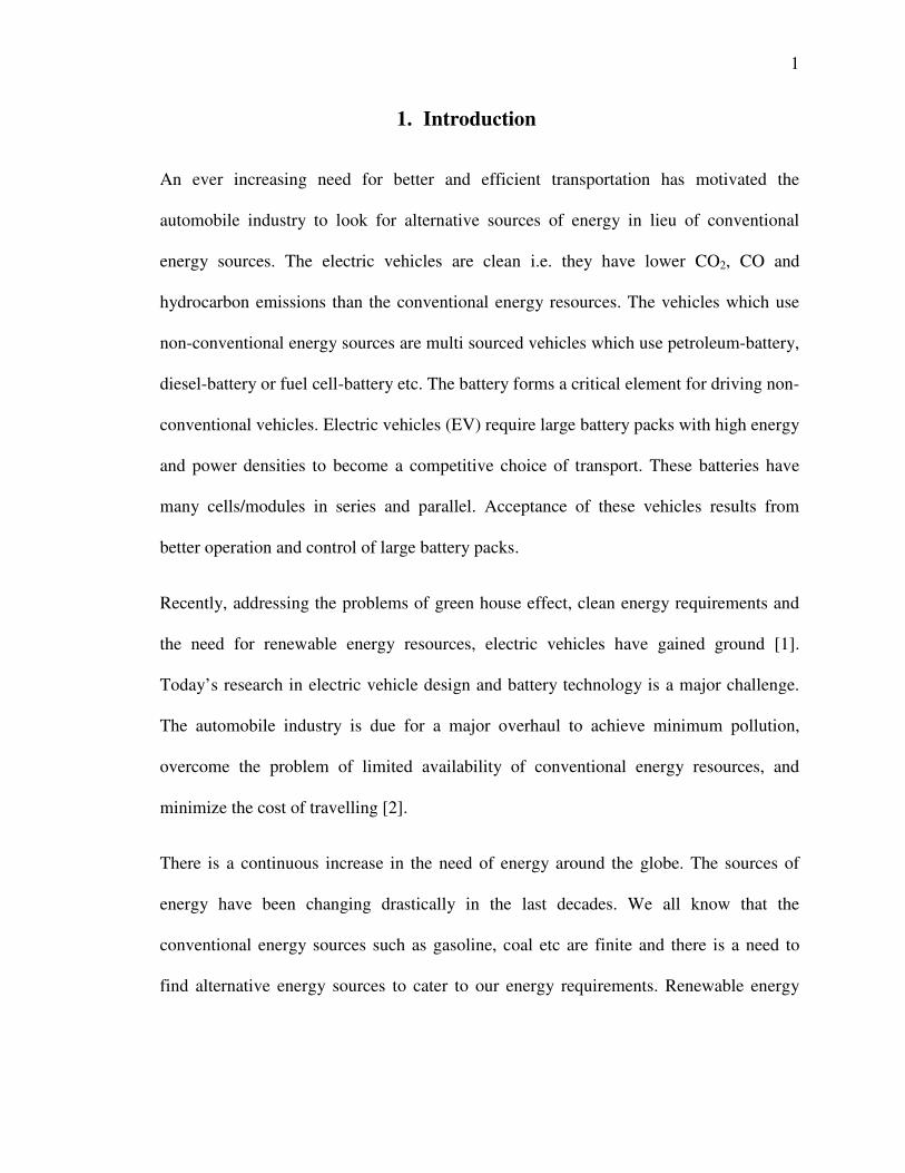
resources have been contributing to the energy requirement. An effort to reduce the cost

of renewable energy sources like wind energy and solar energy is the need of the hour.

Fig. 1.1. Energy Information

USA Energy Information Administration Annual Energy Review 2009 (Aug 2010)

In Fig. 1.1, it can observed that the major source of energy for transportation is petroleum

i.e. 94% and only 3% comes of the energy from renewable energy sources [3]. The major

reason for this is the availability of renewable energy sources to drive the vehicles on

their own is not practical a option; whatever comes in the 3% is the energy from the grid

which is stored in the electric vehicle battery or electric locomotives which are connected

to the grid. Hence, to satisfy our energy need we have to depend on the energy from the

3

grid and limit the use of internal combustion engine. But, the current electricity has many

limitations and there are limitations on the infrastructure support.

It is our primary requirement if we have to move from non-renewable energy resources to

renewable energy resources we should have a very robust grid which can support the

energy needs. The grid should be able to support the additional loads from the electric

vehicles. Also, it should be able to meet the variable energy load which varies depending

on the time and the season. The cost of energy should not increase with the increase an

energy requirement and the grid should also not fail under additional loads.

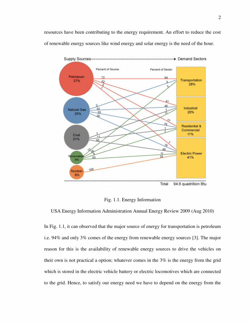
Fig. 1.2. Smart Grid Architecture

The modern grid, which incorporates the provision for advanced loads and providing

energy efficient solution is depicted in Fig. 1.2. The modern grid is also known as “smart

grid” as it can keep a track on the energy price per hour, source of energy during an hour

and it would be a self healing grid which solves problems like voltage fluctuations, black

4

outs etc. It can fix its own operating fixed voltage and can correctly monitor the high

voltage on the grid. The best feature in the grid is that a user can be the customer for

energy or can sell the excess energy, i.e. which means that there would be a two way

interaction between the user and grid. This will help in monitoring energy levels at peak

hours. We will limit our application of the smart grid to electric vehicles and their

operation.

1.1 Hybrid and Plug-in Hybrid Electric Vehicles

Vehicles, which consist of two sources of energy in combination for propulsion are

termed as the hybrid or plug-in hybrid electric vehicles. The source of energy used for

driving the vehicles can be a combination for any of the following: diesel, gasoline,

battery, bio-fuels, fuel cells etc. Hybrid-vehicles are recognized in today’s market and are

being appreciated for their low operation cost and low exhaust emissions. Hybrid-

vehicles with a combination of diesel and battery are less efficient than gasoline and

battery combination. Hybrid-vehicles with fuel cell and battery are more efficient than

gasoline and battery hybrid-vehicle, but they are commercially less successful because of

the flammable properties of hydrogen. Also, hydrogen has storage limitations. Hence,

more work is required on this front so as to make hydrogen and battery combination

successful. Hybrid and Plug-in hybrid electric vehicles are classified based on their

power train configuration

• Parallel hybrid

• Series hybrid

• Power split hybrid

5

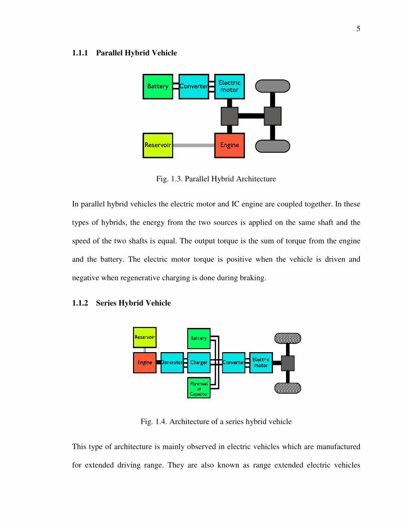
1.1.1 Parallel Hybrid Vehicle

Fig. 1.3. Parallel Hybrid Architecture

In parallel hybrid vehicles the electric motor and IC engine are coupled together. In these

types of hybrids, the energy from the two sources is applied on the same shaft and the

speed of the two shafts is equal. The output torque is the sum of torque from the engine

and the battery. The electric motor torque is positive when the vehicle is driven and

negative when regenerative charging is done during braking.

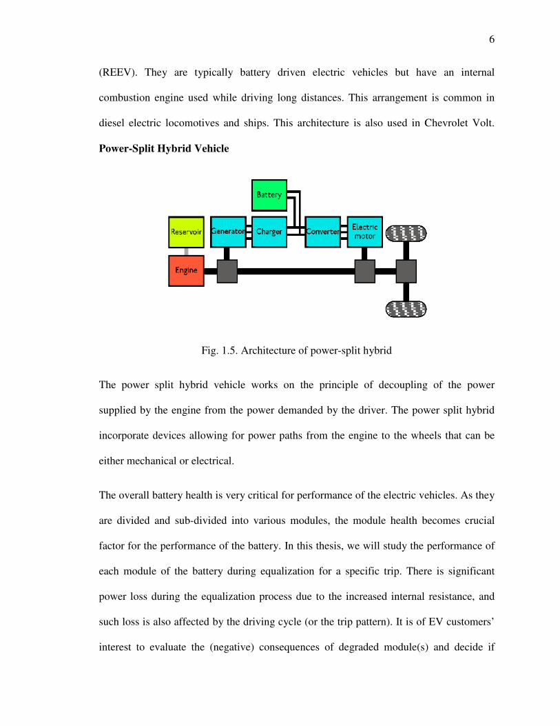
1.1.2 Series Hybrid Vehicle

Fig. 1.4. Architecture of a series hybrid vehicle

This type of architecture is mainly observed in electric vehicles which are manufactured

for extended driving range. They are also known as range extended electric vehicles

6

(REEV). They are typically battery driven electric vehicles but have an internal

combustion engine used while driving long distances. This arrangement is common in

diesel electric locomotives and ships. This architecture is also used in Chevrolet Volt.

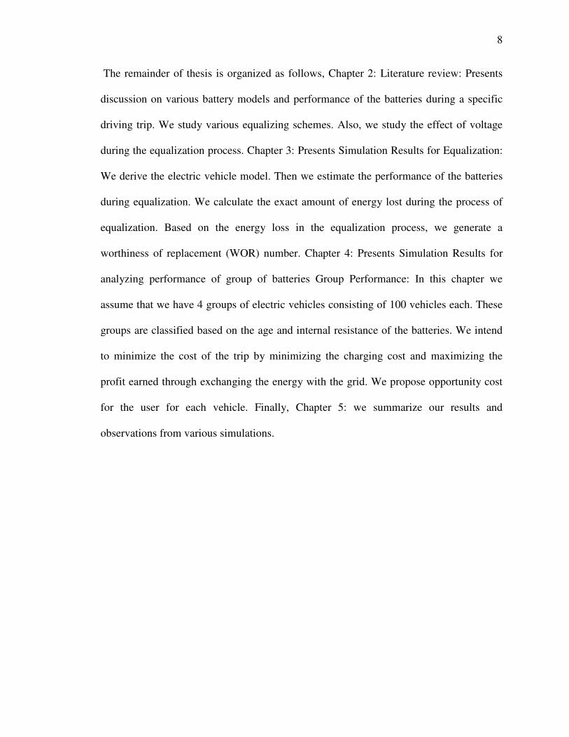
Power-Split Hybrid Vehicle

Fig. 1.5. Architecture of power-split hybrid

The power split hybrid vehicle works on the principle of decoupling of the power

supplied by the engine from the power demanded by the driver. The power split hybrid

incorporate devices allowing for power paths from the engine to the wheels that can be

either mechanical or electrical.

The overall battery health is very critical for performance of the electric vehicles. As they

are divided and sub-divided into various modules, the module health becomes crucial

factor for the performance of the battery. In this thesis, we will study the performance of

each module of the battery during equalization for a specific trip. There is significant

power loss during the equalization process due to the increased internal resistance, and

such loss is also affected by the driving cycle (or the trip pattern). It is of EV customers’

interest to evaluate the (negative) consequences of degraded module(s) and decide if

7

replacement is necessary. The decision of replacement thus relies on a combination of

both diagnosis of physical conditions and economical payback.

Any electric vehicle user desires to know: 1) how much energy loss would be induced for

a specific driving trip based on the knowledge of module characteristics within the

battery pack, and 2) for the given battery pack, what energy efficiency will the user

achieve by replacing certain degraded module or cell with a healthy one. We can

investigate the battery health from the internal resistance of the battery pack.

We also know that with the rise in internal resistance, the battery performance deviates

and degrades. This results in a rise in the charging time and degraded performance of the

battery pack during the driving cycle. Also, with the charging scenario in the smart grid

we have the opportunity to decide the charging times, and supply energy to the grid to

decrease the cost of the trip. A prior knowledge of the trip/driving cycle, cost of energy

on the grid, the battery internal resistance and the energy requirement of the trip enables

us to decide the charging and discharging times.

In this thesis, we propose to quantitatively measure the evaluation of module based

replacement, named as the “Worthiness of Replacement” (WOR). For a given driving

cycle, the WOR of a specific battery pack is defined as the ratio of the state of charge

(SOC) change of the current battery pack to that after replacing certain module with a

healthy module of nominal specifications. We will measure the Opportunity Cost (OC)

for a given vehicle classified as per their age. The opportunity cost for the vehicles is the

ratio of the average cost of charging to the average cost of exchange of energy to the grid.

8

The remainder of thesis is organized as follows, Chapter 2: Literature review: Presents

discussion on various battery models and performance of the batteries during a specific

driving trip. We study various equalizing schemes. Also, we study the effect of voltage

during the equalization process. Chapter 3: Presents Simulation Results for Equalization:

We derive the electric vehicle model. Then we estimate the performance of the batteries

during equalization. We calculate the exact amount of energy lost during the process of

equalization. Based on the energy loss in the equalization process, we generate a

worthiness of replacement (WOR) number. Chapter 4: Presents Simulation Results for

analyzing performance of group of batteries Group Performance: In this chapter we

assume that we have 4 groups of electric vehicles consisting of 100 vehicles each. These

groups are classified based on the age and internal resistance of the batteries. We intend

to minimize the cost of the trip by minimizing the charging cost and maximizing the

profit earned through exchanging the energy with the grid. We propose opportunity cost

for the user for each vehicle. Finally, Chapter 5: we summarize our results and

observations from various simulations.

9

2. Literature Review

In this chapter the electric vehicle model is reviewed. We formulate all the equations

which are useful to model an electric vehicle under driving conditions. Also, various

types of batteries and battery models are studied with their application. Large battery

packs have varied properties and performance under same or different operating

conditions. They are subjected to equalization to optimize and improve their

performance. We review current controlled as well as voltage controlled equalization

schemes.

2.1 Electric Vehicle Model

In order to derive expressions for motor driving torque and motor driving current, we

need propulsion dynamics first. Vehicle propulsion dynamics is dependent on

aerodynamic force, acceleration force on the vehicle, and rolling resistance force.

2.1.1 Aerodynamic Force

The aerodynamic force is the force due to friction on the moving body from the air. This

force takes into consideration the protruding shapes and surfaces, ducts passages,

spoilers, frontal area of the vehicle.

21

2ad dF AC vρ=

(2.1)

where, ρ is the air density, A is frontal area, Cd is the coefficient of drag and v is the

velocity of the vehicle.

10

A good design can effectively reduce the force due to drag by reducing the frontal area

from the shape and also reduce coefficient of drag.

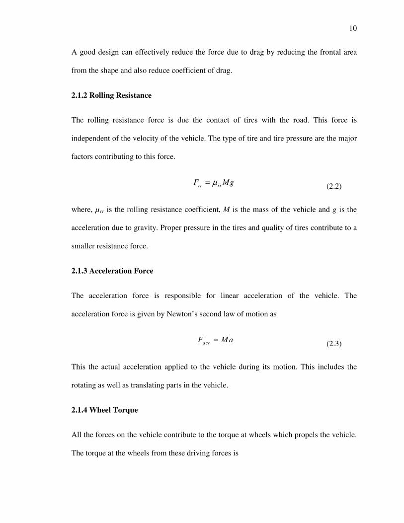
2.1.2 Rolling Resistance

The rolling resistance force is due the contact of tires with the road. This force is

independent of the velocity of the vehicle. The type of tire and tire pressure are the major

factors contributing to this force.

where, µ rr is the rolling resistance coefficient, M is the mass of the vehicle and g is the

acceleration due to gravity. Proper pressure in the tires and quality of tires contribute to a

smaller resistance force.

2.1.3 Acceleration Force

The acceleration force is responsible for linear acceleration of the vehicle. The

acceleration force is given by Newton’s second law of motion as

This the actual acceleration applied to the vehicle during its motion. This includes the

rotating as well as translating parts in the vehicle.

2.1.4 Wheel Torque

All the forces on the vehicle contribute to the torque at wheels which propels the vehicle.

The torque at the wheels from these driving forces is

µ=rr rrF Mg (2.2)

=accF Ma (2.3)

11

( )= + +wh ad rr accT F F F r (2.4)

where, Fad is the aerodynamic force, Frr is the rolling resistance force, Facc is the

accelerating force, and r is the radius wheel.

2.1.5 Motor Torque

In case of electric vehicles the output torque requirement is satisfied by the electric

motor. To complete specified motion of the wheel electric motor produces torque at the

motor shaft. The torque at the motor shaft is

η

=⋅

whm

g

TT

G

(2.5)

where, Twh is the torque at the wheels, Tm is the torque at the motor, G is the gear ratio

and ηg is the gear efficiency.

2.2 Electric Motor Model

Modeling electric motor to satisfy the required motion of the vehicle is the primary

requirement of the electric vehicle. The propulsion of the electric vehicle is completely

dependent on the electric motor. The factors which are considered for electric vehicles

are acceleration requirement, speed requirements, life of the motor and regeneration

requirements. Also, there are limiting factors for modeling the performance of the motors

which are motor torque requirement, angular speed and acceleration. The performance of

the motor helps to increase the tire life. It also keeps a check on the maximum speed the

vehicle can be driven. If these design requirements are not considered, the performance

of the electric vehicle is adversely affected.

12

We have the design requirements and the expected performance from the electric motor.

The parameters to design the electric motor are resistance (Ω), motor inductance (L),

back emf constant (volt-sec/rad), torque constant (N-m/a), rotor inertia (kg*m2) and

mechanical damping. The automotive parameters considered are vehicle damping

(friction), transmission dynamics, gear ratio and tire friction on the pavement. The

electric motor is scaled based on motor speed and torque range. We have limit on the

torque and speed of the motor. Also, to safeguard motor from burning out, we set a limit

for maximum current and voltage. Efficiency of the motor varies with motor torque,

power and motor size. Thus interpolating efficiency with the motor torque and speed is

used calculate input and output power of the motor at wheels.

The input power required by the motor from the battery is

where, Pi is the input power and η0 is the motor efficiency

where, P0 is the output power, PW is the power required at wheels and η is the gear

efficiency

The type of electric motor selected for electric vehicle is dependent on the type of motor

used. AC motors have robust performance, but they fail to react to sudden changes in

speed; DC motors perform ideally under sudden acceleration and deceleration. Therefore

0

0

i

PP

η=

(2.6)

0W

PP

η=

(2.7)

13

the choice of motor is a tradeoff between performance during acceleration and running

under high speeds. Following are some of the typical configurations of permanent magnet

synchronous motors used for electric racing cars

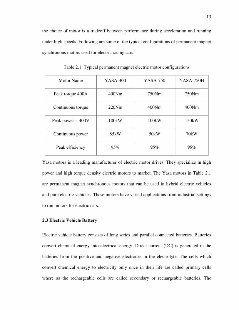
Table 2.1. Typical permanent magnet electric motor configurations

Motor Name YASA-400 YASA-750 YASA-750H

Peak torque 400A 400Nm 750Nm 750Nm

Continuous torque 220Nm 400Nm 400Nm

Peak power ~ 400V 100kW 100kW 150kW

Continuous power 85kW 50kW 70kW

Peak efficiency 95% 95% 95%

Yasa motors is a leading manufacturer of electric motor drives. They specialize in high

power and high torque density electric motors to market. The Yasa motors in Table 2.1

are permanent magnet synchronous motors that can be used in hybrid electric vehicles

and pure electric vehicles. These motors have varied applications from industrial settings

to run motors for electric cars.

2.3 Electric Vehicle Battery

Electric vehicle battery consists of long series and parallel connected batteries. Batteries

convert chemical energy into electrical energy. Direct current (DC) is generated in the

batteries from the positive and negative electrodes in the electrolyte. The cells which

convert chemical energy to electricity only once in their life are called primary cells

where as the rechargeable cells are called secondary or rechargeable batteries. The

14

rechargeable batteries can be charged by reversing the chemical reactions in the battery.

There by bringing the batteries to their original state of charge. The batteries used for

electric vehicles are rechargeable batteries which propel the electric motor. Electric

vehicle batteries undergo deep discharge so as to satisfy the need of power. Hence the

electric vehicle batteries should have high ampere-hour (Ah) capacity. The following are

the characteristics the electric vehicle must have:

• High energy density

• High calendar life

• Low cost batteries

• Low replacement cost

• High reliability

• Robustness

• Low weight and smaller sizes

• Higher power to weight ratio

The major drawback for electric and plug-in hybrid electric vehicles is their range of

travel. Vehicle with internal combustion engine (ICE) have no limiting range for travel

whereas electric vehicles have maximum of 30-350 miles all electric range. Electric

vehicles have lower specific energy which results in poor performance during initial

acceleration compared to internal combustion engines. This means that the electric

vehicles have lower initial acceleration as the batteries are restricted from performing

15

sudden deep discharging cycles which degrade the battery life, and also the motor

responds slowly to changes in acceleration. On the other hand, the internal combustion

engines can provide power efficiently starting the vehicle from rest without degrading the

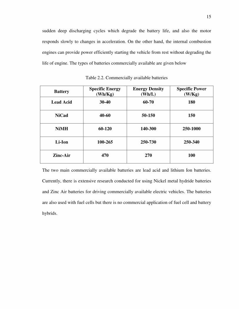
life of engine. The types of batteries commercially available are given below

Table 2.2. Commercially available batteries

The two main commercially available batteries are lead acid and lithium Ion batteries.

Currently, there is extensive research conducted for using Nickel metal hydride batteries

and Zinc Air batteries for driving commercially available electric vehicles. The batteries

are also used with fuel cells but there is no commercial application of fuel cell and battery

hybrids.

Battery Specific Energy

(Wh/Kg) Energy Density

(Wh/L) Specific Power

(W/Kg)

Lead Acid 30-40 60-70 180

NiCad 40-60 50-150 150

NiMH 60-120 140-300 250-1000

Li-Ion 100-265 250-730 250-340

Zinc-Air 470 270 100

16

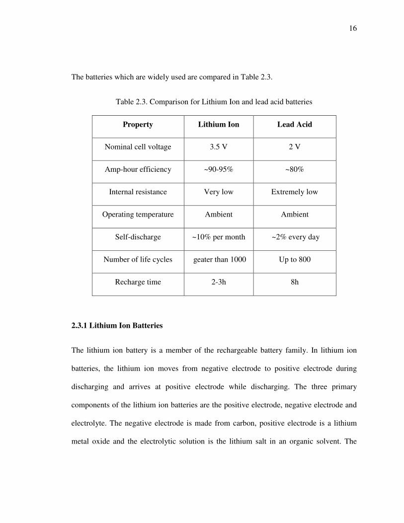
The batteries which are widely used are compared in Table 2.3.

Table 2.3. Comparison for Lithium Ion and lead acid batteries

Property Lithium Ion Lead Acid

Nominal cell voltage 3.5 V 2 V

Amp-hour efficiency ~90-95% ~80%

Internal resistance Very low Extremely low

Operating temperature Ambient Ambient

Self-discharge ~10% per month ~2% every day

Number of life cycles geater than 1000 Up to 800

Recharge time 2-3h 8h

2.3.1 Lithium Ion Batteries

The lithium ion battery is a member of the rechargeable battery family. In lithium ion

batteries, the lithium ion moves from negative electrode to positive electrode during

discharging and arrives at positive electrode while discharging. The three primary

components of the lithium ion batteries are the positive electrode, negative electrode and

electrolyte. The negative electrode is made from carbon, positive electrode is a lithium

metal oxide and the electrolytic solution is the lithium salt in an organic solvent. The

17

direction of the lithium ions change between anode and cathode based on the direction of

the current flow.

Fig. 2.1. Typical initial Lithium ion battery pack

A typical lithium ion battery pack during its early formations is as shown in Fig. 2.1.

Lithium batteries first came into existence in 1970 by M.S. Whittingham, while he

worked for Exxon [4]. The major drawback with the lithium ion batteries is that lithium is

highly explosive and there are safety issues working with lithium ion batteries. The

present form of lithium ion batteries came into existence in 1985, by Akira Yoshino [5].

He assembled lithium ion electrodes, lithium cobalt oxide and carbonaceous electrolyte.

The performance of lithium ion batteries are best suited for applications like electric

vehicle as the batteries are light weight and have high energy density.

2.3.2 Battery Modeling Technique

18

So as to model a particular type and application of the battery with R-C circuits, we must

know the behavior of the battery. The performance of the battery is dependent on 30-40

variables. The model of battery generated is strictly for that specific battery. The models

of batteries are used to understand the performance of the battery and its behavior which

requires the knowledge of fundamental physics and chemistry. Parameters like

temperature, voltage, resistance and current can be measured with greater accuracy.

Based on these parameters we can model the performance of electric vehicle batteries

using lesser complicated R-C circuits. The battery models generate accurate state of

charge (SOC) and open circuit voltage (VOC) of the battery. If the battery SOC or VOC

fall below a certain limit, their characteristics change permanently, this degrades their

performance. The charging and discharging resistance of the batteries is of critical

importance as it the performance determining factor. It can be calculated based on the

type of the battery [6]. Electric vehicle battery model must account for self discharging

resistance and the operating temperature of the vehicle.

The model we consider for our research does not include self discharge resistance as we

do not simulate over long term behavior of the model, in which case this resistance would

be meaningful. Also, we do not account for the effect of temperature on the battery

performance as we assume that the operating range of the temperature is very small i.e.

the operating range of the electric vehicle battery is small.

2.3.3 Battery Equivalent Circuit Representation

The crucial parts for electric vehicles are low power dissipation and maximum battery

run time. An accurate circuit model can solve the problem of predicting and optimizing

battery run time and circuit performance. The dynamic model must account for all

19

dynamic characteristics of the non-linear open circuit voltage, current, temperature, cycle

number and storage time dependent capacity to transient response.

Fig. 2.2. Battery model examples (a) Thevenin electrical model

(b) Impedance based electrical model

We can observe in Fig. 2.2(a) the most basic form of battery equivalent R-C model

connections is shown. The battery consists of a series resistance and a parallel R-C

connection to predict the open circuit voltage and SOC of the battery [7,8]. The major

(a)

(b)

20

drawback of the battery is that it assumes open circuit voltage as constant and this

assumption makes it impossible to predict steady state battery variation [9]. The

electrochemical impedance spectroscopy in Fig. 2.2(b) obtain an AC equivalent

impedance model in the frequency domain and then use a complicated equivalent

network (Zac) to fit the impedance spectra. The drawback for this method is that it’s

difficult, complex and non-intuitive. Also, they only work for fixed SOC and temperature

setting [10].

Fig. 2.3. Runtime Based Electrical Battery Models

The Runtime based battery model is as shown in Fig. 2.3 use a complex circuit network

and a DC voltage [11]. They cannot predict voltage response with varying loads and

runtime voltage [12].

In 2007, Vasebi et al developed an extended kalman filter for estimating the SOC which

was a nonlinear estimating technique for accurate prediction performance of the SOC.

21

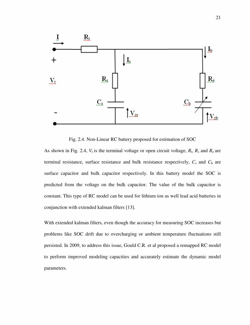
Fig. 2.4. Non-Linear RC battery proposed for estimation of SOC

As shown in Fig. 2.4, Vt is the terminal voltage or open circuit voltage, Rt, Rs and Re are

terminal resistance, surface resistance and bulk resistance respectively, Cs and Cb are

surface capacitor and bulk capacitor respectively. In this battery model the SOC is

predicted from the voltage on the bulk capacitor. The value of the bulk capacitor is

constant. This type of RC model can be used for lithium ion as well lead acid batteries in

conjunction with extended kalman filters [13].

With extended kalman filters, even though the accuracy for measuring SOC increases but

problems like SOC drift due to overcharging or ambient temperature fluctuations still

persisted. In 2009, to address this issue, Gould C.R. et al proposed a remapped RC model

to perform improved modeling capacities and accurately estimate the dynamic model

parameters.

22

Fig. 2.5. Remapped battery model

In Fig. 2.5, Rp is the self discharge resistance which is very large compared to the overall

resistance of the battery. Cn and Rn are capacitor and resistor in series in the model. The

change in Cp over a considerable period of time will be the representation of the state of

health (SoH) for the battery. Ri is the resistance of the battery terminals and inter-cell

connections. Cp and Rp are capacitor and resistors in parallel.

2.3.4 Battery Equalization

A serious problem which affects battery performance is the voltage across each battery.

Electric vehicle consists of more than 80-100 cells in each battery. The cells have varying

internal properties which results in variation in the open circuit voltage. Since SOC is

based on the open circuit voltage, if there are errors present in the open circuit voltage

measurement, there will be errors in SOC measurements. Also, the battery performance is

degraded if wrong measurements for SOC are considered for the battery. To avoid

23

uneven performance of large group of batteries, they are forced to exhaust energy in the

heat sink. This results in loss of energy and increases the cost of travelling and utilizing

batteries.

To address the problem of variation of voltage in series connected cells for electric

vehicles, many techniques have been developed [14]. To make the equalization process

implementable, cost effective and to keep the voltage and current stresses low, modular

charge equalization process was developed by H. Park et al. In this technique, the battery

pack is divided in many small modules and then intra-module equalizer and outer module

equalizer are designed [15].

Fig. 2.6. Multi-winding transformer (a) Conventional Approach (b) Modularized Approach

A battery pack with series connected cells is shown in Fig. 2.6(a). The same battery pack

with modularized design pattern is shown in Fig. 2.6(b). The battery pack is divided into

(a) (b)

24

maximum number of 8-10 cells per module, many modules in series form a battery pack.

With the formation of modules we overcome problem of mismatched inductance leakage

and implementation of the modules becomes easier.

2.4 Smart Grid

The success of implementing hybrids into the market largely depends on the

infrastructure of charging the vehicles from the grid [16]. To build a strong grid network,

renewable energy sources like wind energy, solar energy, batteries etc are used along

with the conventional sources of energy. Continuous effort is made to lower the cost of

energy generation to support the grid [17]. This has led to novel concepts of smart grid

where there could be energy exchange from the grid to the end user and from the end user

to the grid [18,19]. Not only we can predict the load and price of the energy for the next

day, but we can identify the source of power during a specific time of the day. This

concept could be very beneficial for setting up the charging algorithms for electric

vehicles [20,21]. The concept of smart grid has motivated researchers to optimize the cost

of operation of the grid and its maintenance. The cost of producing and supplying

electricity from various sources is minimized using the available renewable and non-

renewable sources of energy and the nature of load which is applied on the grid. The load

on the grid is time dependent, so does the cost of energy which varies with time, season

and many other factors [22]. It is widely known that the load on the grid is lowest during

nights which bring the prices of the electricity to its lowest, whereas the load during the

day time is the highest, which forces the prices to its maximum values [23].

25

Increasing the number of electric vehicles in the market will compel the grid to support

the additional load. The charging time for electric vehicles is mostly during the nights.

The grids have lower loads during nights as compared during the day. Also, the price of

electricity during the night is lowest which helps to minimize the charging cost [24].

Hence, the grid load and electricity price could be regulated.

Electric and plug-in hybrid vehicles use large battery packs, containing batteries in series

and parallel arrangement to obtain required battery configuration. Electric vehicles can

now-a-days travel more than 100 miles with one complete charging cycle which is

significantly more than daily commuting distance from home to office and back home.

This allows us to look at the electric vehicles as the potential supplier of energy to the

grid. These batteries have independent cell/module properties because of their

manufacturing process and variability in the processes they undergo [25]. Also, they

degrade and respond independently to different conditions to which they are exposed.

Batteries deteriorate with age and their performance drops down significantly [26]. The

knowledge of the trip to be travelled, the age of the battery and the time required for

charging will he help us identify the amount of energy available with any vehicle selected

at random. This helps to determine the amount of energy that is available from the

batteries that can be exchanged with the grid.

26

3. Simulation Results for Equalization

In this chapter we discuss electric vehicle under various driving conditions. We model the

battery which is exposed to equalization process during the driving cycle. We calculate

the loss for battery for two module equalization process and then with three module

battery. We calculate the “Worthiness of Replacement” (WOR) for two module and three

module case. We also estimate the loss in the batteries with higher internal resistance. We

can quantify the loss in the process of equalization.

3.1 Electric Vehicle and Motor

D.C. motors have limitations on life and they are not robust as to A.C. motors. The A.C.

motors have a sluggish response, whereas D.C. motors have faster response. These

drawbacks are overcome by permanent magnet synchronous motor (PMSM). The PMSM

motors are robust and their performance for initial acceleration is better than the A.C.

motors. The motor we use for our research is permanent magnet synchronous motor with

a gear box transmission. The motor is a 4-pole 560V synchronous motor with rated speed

of ~5000rpm. The torque limits were ~140N-m and ~160N-m during driving and braking

respectively. The following are the electric vehicle parameters used by us in our

simulation study:

27

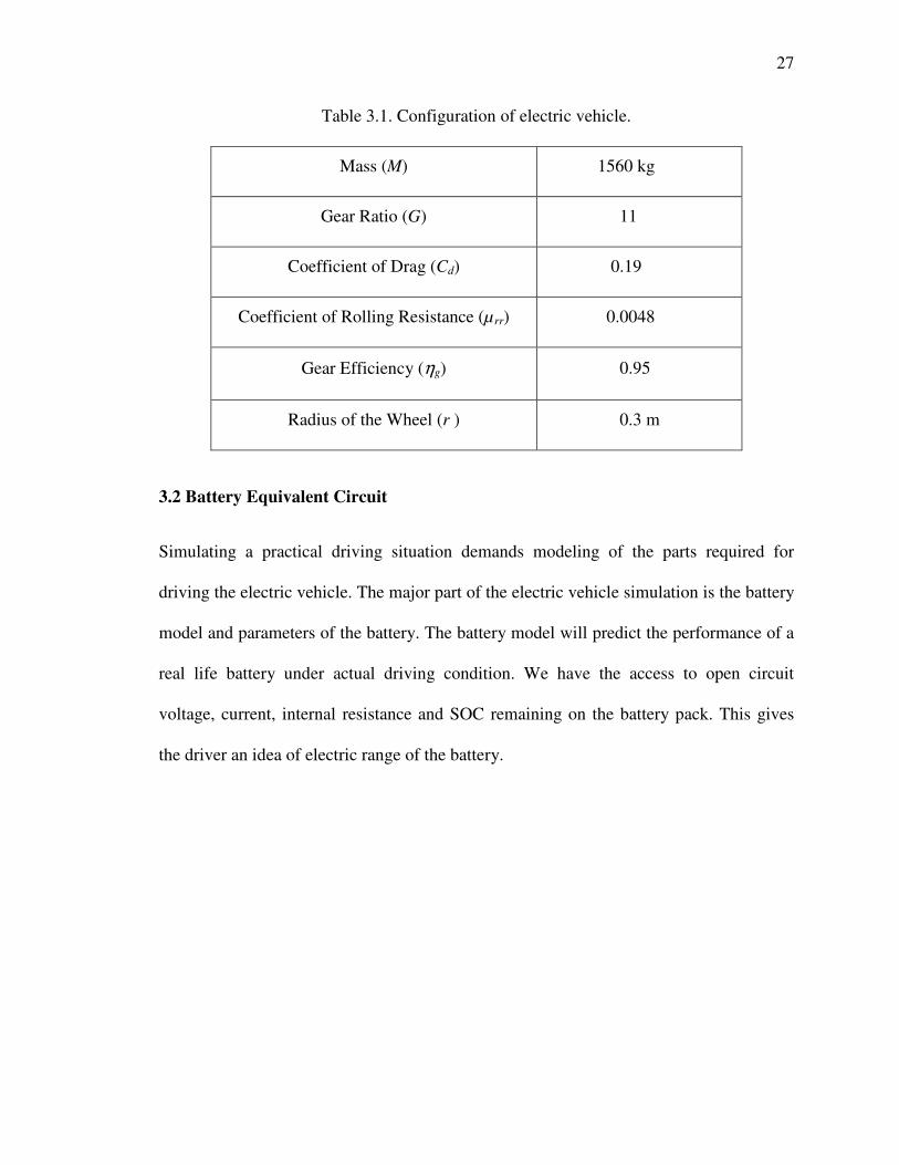
Table 3.1. Configuration of electric vehicle.

Mass (M) 1560 kg

Gear Ratio (G) 11

Coefficient of Drag (Cd) 0.19

Coefficient of Rolling Resistance (µ rr) 0.0048

Gear Efficiency (ηg) 0.95

Radius of the Wheel (r ) 0.3 m

3.2 Battery Equivalent Circuit

Simulating a practical driving situation demands modeling of the parts required for

driving the electric vehicle. The major part of the electric vehicle simulation is the battery

model and parameters of the battery. The battery model will predict the performance of a

real life battery under actual driving condition. We have the access to open circuit

voltage, current, internal resistance and SOC remaining on the battery pack. This gives

the driver an idea of electric range of the battery.

28

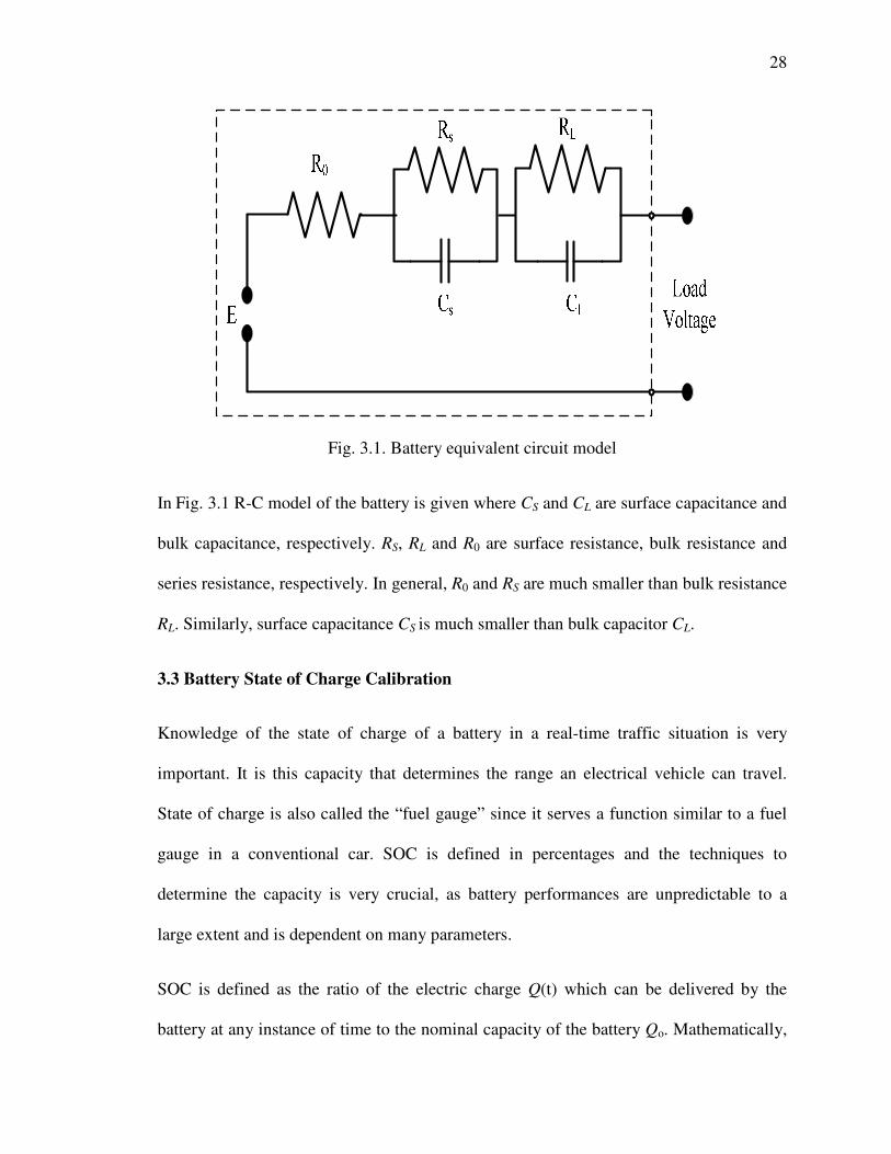
Fig. 3.1. Battery equivalent circuit model

In Fig. 3.1 R-C model of the battery is given where CS and CL are surface capacitance and

bulk capacitance, respectively. RS, RL and R0 are surface resistance, bulk resistance and

series resistance, respectively. In general, R0 and RS are much smaller than bulk resistance

RL. Similarly, surface capacitance CS is much smaller than bulk capacitor CL.

3.3 Battery State of Charge Calibration

Knowledge of the state of charge of a battery in a real-time traffic situation is very

important. It is this capacity that determines the range an electrical vehicle can travel.

State of charge is also called the “fuel gauge” since it serves a function similar to a fuel

gauge in a conventional car. SOC is defined in percentages and the techniques to

determine the capacity is very crucial, as battery performances are unpredictable to a

large extent and is dependent on many parameters.

SOC is defined as the ratio of the electric charge Q(t) which can be delivered by the

battery at any instance of time to the nominal capacity of the battery Qo. Mathematically,

29

the state of charge is given as below

( )

( )o

Q tSOC t

Q= (3.1)

The charge remaining on the battery varies with time and various environmental factors.

Also, the ageing of the battery should be taken into consideration. The following are

different SOC measurement techniques :

1. Direct Measurement technique

2. SOC from the specific gravity measurements

3. Internal Impedance of the battery

4. Coulomb counting (Current measurement)

5. SOC based on the open circuit voltage

The deterministic techniques mentioned above can estimate the SOC accurately based on

the application. The most efficient and accurate techniques for estimating SOC for

electric vehicles are based on open circuit voltage and coulomb counting. Coulomb

counting can be used for estimating SOC for a short period of time like during a day or

over a span of few months [27]. Open circuit voltage of the battery is an accurate

measure for the health of the battery, so the variation of the SOC with the age of the

battery is accounted in the open circuit voltage. Thus, we use SOC measurement based on

open circuit voltage throughout the life of the battery.

We drive our electric vehicle for a specific driving trip. We do not consider the change in

battery of the electric vehicle throughout its life. We can efficiently consider coulomb

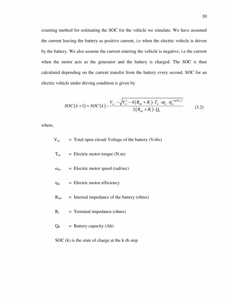
30

counting method for estimating the SOC for the vehicle we simulate. We have assumed

the current leaving the battery as positive current, i.e when the electric vehicle is driven

by the battery. We also assume the current entering the vehicle is negative, i.e the current

when the motor acts as the generator and the battery is charged. The SOC is then

calculated depending on the current transfer from the battery every second. SOC for an

electric vehicle under driving condition is given by

( ) ( )( ) ( )

( )

sgn2

int

int

41

2

mT

oc oc t m m m

t b

V V R R TSOC k SOC k

R R Q

ω η−

− − + ⋅ ⋅ ⋅+ = −

+ ⋅ (3.2)

where,

Voc = Total open circuit Voltage of the battery (Volts)

Tm = Electric motor torque (N.m)

ωm = Electric motor speed (rad/sec)

ηm = Electric motor efficiency

Rint = Internal impedance of the battery (ohms)

Rt = Terminal impedance (ohms)

Qb = Battery capacity (Ah)

SOC (k) is the state of charge at the k-th step

31

3.4 Battery Equalization Scheme

As the voltage in a single cell is quite low, for high voltage applications like EV, battery

modules and packs are made via serial and parallel combinations of the cells [28].

Variations are inevitable in the internal resistances of the battery cells and modules. The

variation in the internal resistance is caused by extrinsic or intrinsic cell properties,

contact resistance among cells, or temperature gradient because of improper thermal

management accounts for battery imbalance. The variation in the internal resistance

causes variations in the SOC and degrades the cell [29]. The battery life can be

significantly affected by the imbalance among modules or cells due to the associated

over-charging or over-discharging. Hence, equalizing the modules or cells is important

for acquiring the maximum achievable power and extending the battery life [30,31].

32

Fig. 3.2. Battery Equalization Circuit

In this study, the voltage equalization scheme by Lee and Cheng is adopted [32] with a

two-module situation shown in Fig. 3.2. The voltage of each module determines the

direction of energy transfer between the two modules with proper operation of the

MOSFET switches Q1 and Q2. L1 and L2 are two uncoupled inductors, while C0 is an

energy transferring capacitor.VB1 and VB2 are battery voltages for modules (or cells) 1 and

2, respectively. For normal condition, VC1=VB1+VB2. The ideal condition is VB1 =VB2,

although this can seldom be the case in realistic operation. The operational scenario for a

PWM is shown below.

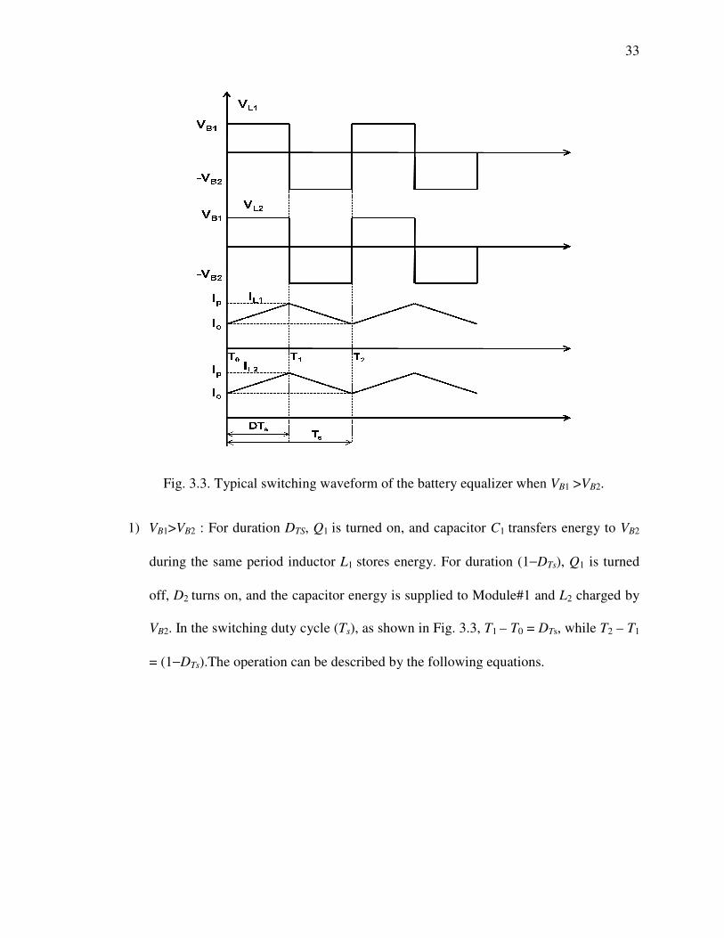
Fig. 3.3. Typical switching waveform of the battery equalizer when

1) VB1>VB2 : For duration

during the same period inductor

off, D2 turns on, and the

VB2. In the switching duty cycle (

= (1−DTs).The operation can be described by the following equations.

Typical switching waveform of the battery equalizer when

ation DTS, Q1 is turned on, and capacitor C1 transfers energy to

during the same period inductor L1 stores energy. For duration (1−D

and the capacitor energy is supplied to Module#1 and

. In the switching duty cycle (Ts), as shown in Fig. 3.3, T1 – T0 = D

).The operation can be described by the following equations.

33

Typical switching waveform of the battery equalizer when VB1 >VB2.

transfers energy to VB2

DTs), Q1 is turned

and L2 charged by

DTs, while T2 – T1

).The operation can be described by the following equations.

34

a) For t∈[T0, T1], Q1 is turned on, which implies

0

22 2 2

0

1( ) ( )

tL

B LT

diV t L i d

dt Cτ τ= − + ∫

2 0 0 ( )Li T I=

(3.4)

b) For t∈[T1, T2], Q1 is turned off and Q2 is turned on, which implies

22 2

( )( ) = − L

B

di tV t

dtL

2 2( )L Pi T I=

(3.6)

Equations (9) through (13) describe the voltages VB1 and VB2 dynamics during one duty

cycle of PWM operation. Ip is the peak current during the operation cycle DTs. The

currents in the inductor IL1 and IL2 are given by

By varying the switching frequency, the equalization scheme can be implemented in

continuous current or discontinuous inductor current mode. During the equalization

11 1

( )( ) = L

B

di tV t

dtL

1 0 0( )Li T I= (3.3)

2

1

21 1 1

0

( ) 1( ) ( )

TL

B LT

di tV t L i d

dt Cτ τ= + ∫

1 1( ) =L P

i T I

(3.5)

2 21 11

1

1 1

1(1 )

2

−= + −

c BBL s

V VVI D D T

L L (3.7)

2 21 2 2

22 2

1(1 ) (1 )

2

−= − + −

c B BL s

V V VI D D T

L L (3.8)

35

process, the weak cell is charged by a strong cell to balance the energy level of both the

cells. In our study battery 1 is at higher energy level than battery 2.

2) VB1<VB2: The operation is controlled by the switching Q2 and D1 in similar fashion as

case 1, and similar equations would apply.

36

3.5 Worthiness of Replacement

The concept of worthiness of replacement (WOR) is applied to the battery pack after the

battery is equalized and the trip is complete. As mentioned earlier, though equalization is

unavoidable, but WOR projects the exact loss of energy in the trip. This analysis would

be the decision making factor for projection of completion of the trip as the onboard

energy is calculated. The WOR is defined as

( )

SOC Change of Current Battery PackWOR

Battery Pack SOC Change with Certain Module s Replaced

=

(3.9)

Equation 3.7 and 3.8 can be enhanced by some averaging operation, for example for

actual or predicted trips of certain number of days. The traffic is stochastic in nature as

driving behavior such averaging will be helpful to obtain more reliable result for

evaluation purpose.

37

3.6 Driving Cycle

We require motor speed and motor torque to study the simulation behavior of the battery.

We start the trip at 124 West Freistadt Road in Thiensville, while the destination is 3200

North Cramer Street in Milwaukee. This is a representative of an ideal driving cycle

which consists of highways, street roads, stop and signs and traffic lights, so we have

decided to use this driving cycle for our simulations.

Fig. 3.4. Route map of the sample trip

The time for driving trip was ~1614sec. The maximum torque during driving is ~140Nm

while the maximum torque during braking or negative torque is ~160N.m. The trip

includes constant driving speed cycles, constant acceleration cycles and constant

deceleration cycles. This trip includes driving in the city roads, on the freeways. It also

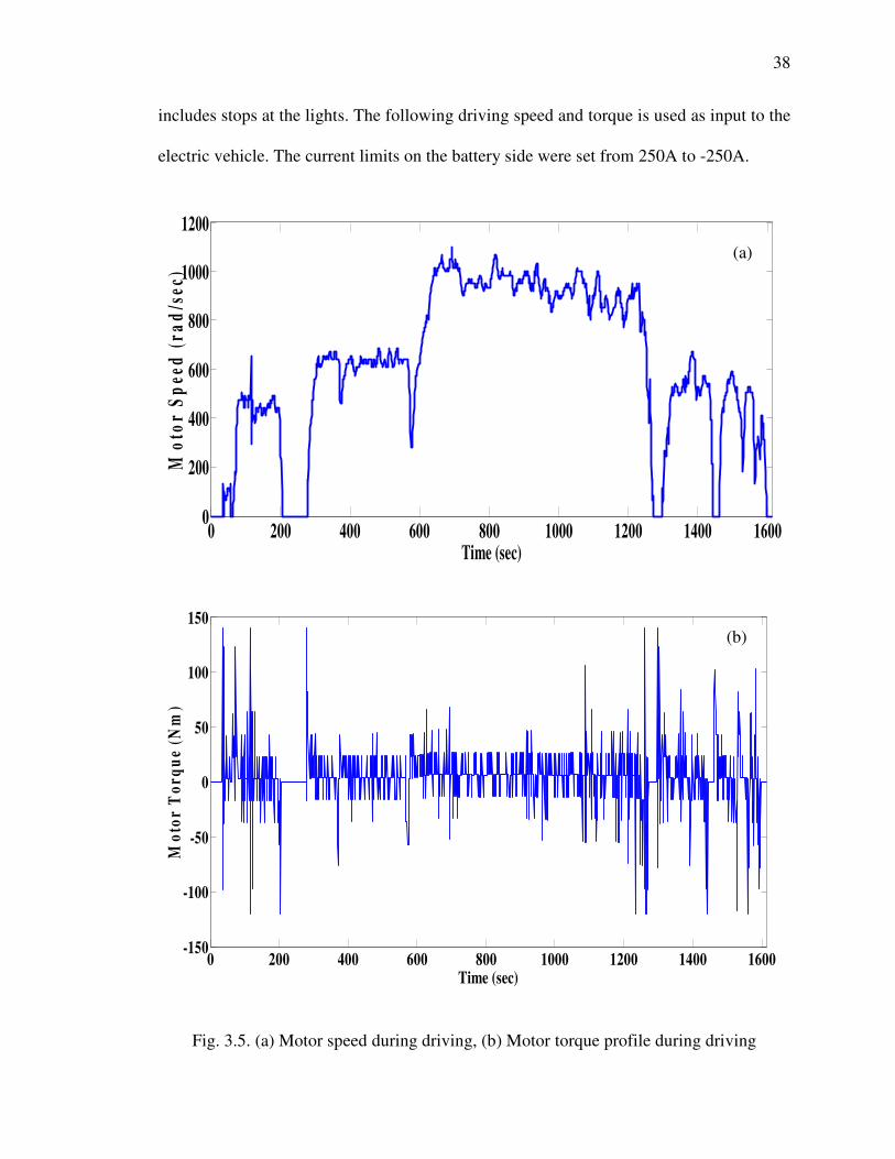
38

includes stops at the lights. The following driving speed and torque is used as input to the

electric vehicle. The current limits on the battery side were set from 250A to -250A.

Fig. 3.5. (a) Motor speed during driving, (b) Motor torque profile during driving

0 200 400 600 800 1000 1200 1400 16000

200

400

600

800

1000

1200

Time (sec)

Mo

tor

Sp

eed

(ra

d/s

ec)

0 200 400 600 800 1000 1200 1400 1600-150

-100

-50

0

50

100

150

Time (sec)

Mo

tor

To

rqu

e (N

m)

(a)

(b)

39

3.7 Two Module Battery Pack

Two battery modules are assumed serially connected. For each module, the capacity

rating is 20Ah, respectively. The upper and lower limits of battery SOC are set to be 80%

and 30%, respectively. Each module consists of 4 sub-modules which have 7 cells in

series, i.e. 28 cells in total, with nominal voltage 3.6V [33]. The voltage across the

battery pack is 201.6V [34], i.e. 100.8 V for each module. The internal resistance values

used in this research are approximately equivalent to the internal resistance values of the

lithium ion batteries from Toyota Prius model. Two cases are simulated with the settings

described below (also summarized in Table 3.2, with B-1 and B-2 representing battery

modules 1 and 2, respectively):

Table 3.2. Initial Conditions of Two Module Simulation Study

Case No.

Battery No.

Voltage(V) Capacity

(Ah) SOC(%)

Internal Resistance

(Ω)

1

B-1 100.8 20 80 0.075

B-2 100.8 20 80 0.075

2

B-1 100.8 20 80 0.075

B-2 100.8 20 65 0.30

40

Case-1: Both modules are in the nominal condition, i.e. having internal resistance of

0.075Ω. Starting from 80% SOC, both modules follow the same discharging trajectory as

shown in Fig. 3.6. The final SOC is 53.52%.

Fig. 3.6. Battery module SOC trajectories for with Case #1with the example driving cycle

Both batteries have the same internal resistance which is 0.075Ω. The batteries are

connected in series which resemble 2 modules. The batteries start discharging at 80%

SOC at the beginning of the trip and end at 53.52% SOC at the end of the trip .The

electric vehicles travels ~27.5 kilometers in 1614 sec. The battery of the vehicle

consumes 26.48% SOC to complete the trip.

0 200 400 600 800 1000 1200 1400 160050

55

60

65

70

75

80

85

Time (sec)

SO

C (

%)

B1

B2

41

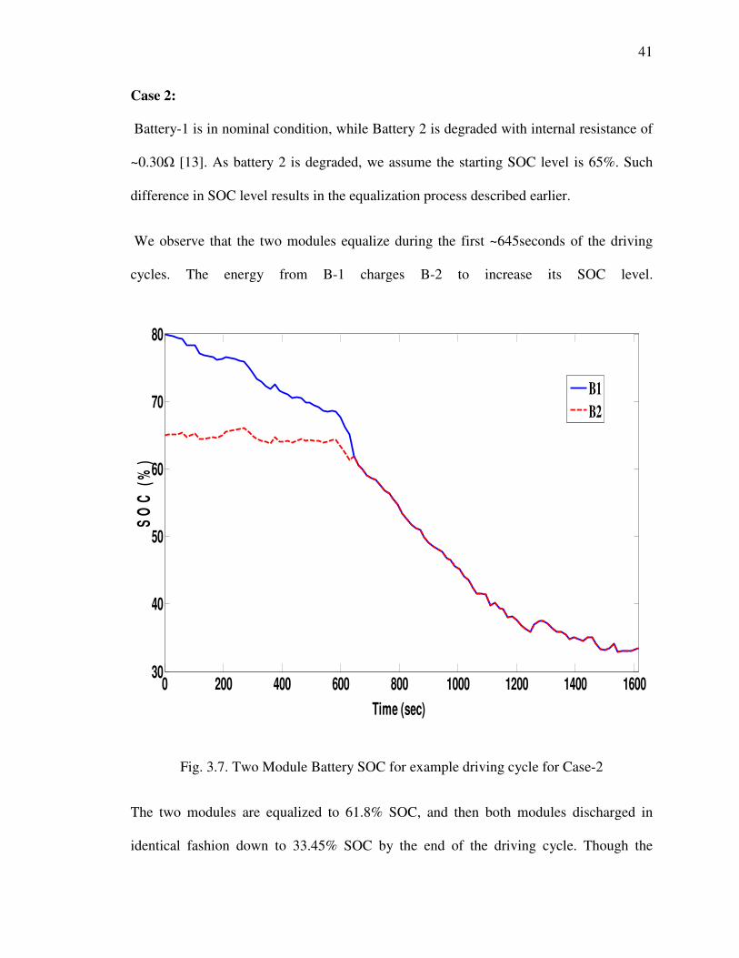
Case 2:

Battery-1 is in nominal condition, while Battery 2 is degraded with internal resistance of

~0.30Ω [13]. As battery 2 is degraded, we assume the starting SOC level is 65%. Such

difference in SOC level results in the equalization process described earlier.

We observe that the two modules equalize during the first ~645seconds of the driving

cycles. The energy from B-1 charges B-2 to increase its SOC level.

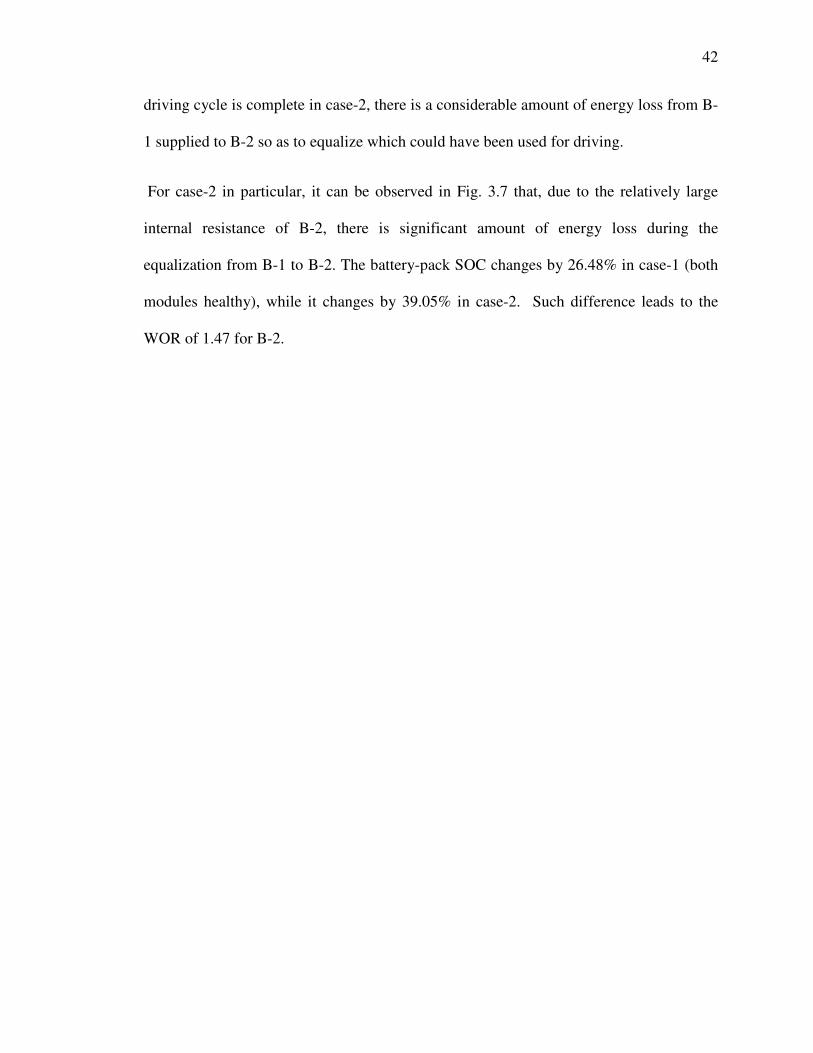
Fig. 3.7. Two Module Battery SOC for example driving cycle for Case-2

The two modules are equalized to 61.8% SOC, and then both modules discharged in

identical fashion down to 33.45% SOC by the end of the driving cycle. Though the

0 200 400 600 800 1000 1200 1400 160030

40

50

60

70

80

Time (sec)

SO

C (

%)

B1

B2

42

driving cycle is complete in case-2, there is a considerable amount of energy loss from B-

1 supplied to B-2 so as to equalize which could have been used for driving.

For case-2 in particular, it can be observed in Fig. 3.7 that, due to the relatively large

internal resistance of B-2, there is significant amount of energy loss during the

equalization from B-1 to B-2. The battery-pack SOC changes by 26.48% in case-1 (both

modules healthy), while it changes by 39.05% in case-2. Such difference leads to the

WOR of 1.47 for B-2.

43

3.8 Three-Module Battery Pack

Simulation is then performed for a battery pack with three modules in series. The

capacity for each module is ~20Ah. The battery pack is composed of three modules. Each

module consists of two serially connected sub-modules of nine cells each, i.e. 18 cells in

series. This configuration results is 64.8V across each module. The overall voltage across

the battery pack is 194.4V. The internal resistance for ideal module is assumed to be

0.054Ω.

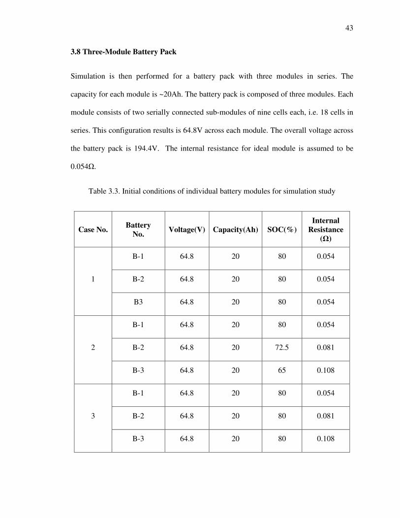
Table 3.3. Initial conditions of individual battery modules for simulation study

Case No. Battery

No. Voltage(V) Capacity(Ah) SOC(%)

Internal Resistance

(Ω)

1

B-1 64.8 20 80 0.054

B-2 64.8 20 80 0.054

B3 64.8 20 80 0.054

2

B-1 64.8 20 80 0.054

B-2 64.8 20 72.5 0.081

B-3 64.8 20 65 0.108

3

B-1 64.8 20 80 0.054

B-2 64.8 20 80 0.081

B-3 64.8 20 80 0.108

44

Three cases are simulated with settings listed in Table 3.3, with B-1, B-2 and B-3

denoting battery modules 1, 2 and 3, respectively.

Case 1:

The batteries have state of charge (SOC) mentioned in Table 3.3.

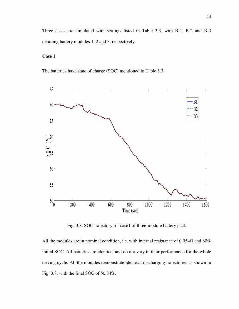
Fig. 3.8. SOC trajectory for case1 of three-module battery pack

All the modules are in nominal condition, i.e. with internal resistance of 0.054Ω and 80%

initial SOC. All batteries are identical and do not vary in their performance for the whole

driving cycle. All the modules demonstrate identical discharging trajectories as shown in

Fig. 3.8, with the final SOC of 50.84%.

0 200 400 600 800 1000 1200 1400 160050

55

60

65

70

75

80

85

Time (sec)

SO

C (

%)

B1

B2

B3

45

Case 2:

B-1 is in nominal condition, B-2 has internal resistance of 0.081Ω with 72.5% initial

SOC, and B-3 has internal resistance of 0.108Ω with 65% initial SOC. This case is

intended to simulate B-2 and B-3 as more degraded modules.

Fig. 3.9. Battery SOC trajectories for three modules for Case 2 of Table 3.3

The driving cycle can be completed with the onboard battery power, there is a

considerable amount of SOC from B-1 supplied to B-2, and that from B-2 supplied to B-

3. Furthermore, due to the relatively higher internal resistances of B-2 and B-3, there is

significant amount of energy loss during the aforementioned equalization processes. This

0 200 400 600 800 1000 1200 1400 160030

40

50

60

70

80

90

Time (s)

SO

C (

%)

B-1

B-2

B-3

46

process results in equalization among the three modules from the start till 1005 seconds,

as shown in Fig. 3.9. In particular, B-1 has higher SOC than B-2 and B-2 has higher SOC

than B-3. The equalization of these three battery modules follow the same logic as

described earlier, i.e. the equalization decision is made for every pair of neighboring

modules based on the comparison of the relevant voltages, which is done by triggering

the associated switches. In the scenario assumed for Case 2, current is discharged from B-

1 to B-2, and current is discharged from B-2 into B-3. All the modules equalize their

SOC to 45.57%. Afterwards, the three modules jointly discharge to 35.34% SOC by the

end of the driving cycle. To complete the same trip, the average SOC drops by 29.16% in

Case-1, while in Case-2, by 37.16%. The corresponding WOR is 1.27.

Case 3:

Case-3 involves an analysis to case 2 except that the starting SOC for all the modules is

identically at 80%. Simulation has also been performed to the situation when battery

module equalization occurs not from the start of the trip, but rather in the middle of the

trip as the SOC difference increases. For this purpose, we consider the same battery

configuration as in Table 3.3 while all the modules have equal starting SOC, i.e. 80%.

The SOC deviates for each module during the first 645 seconds, and then after the

equalization process starts. At that point, the SOC difference between Battery-1 and

Battery-2 was 2.05% and that between Battery-2 and Battery 3 was 1.53%, respectively.

With the equalization process, the modules are equalized to 50.45% by 1050 seconds.

Then the whole battery pack completes the driving cycle at SOC 41.95%.

47

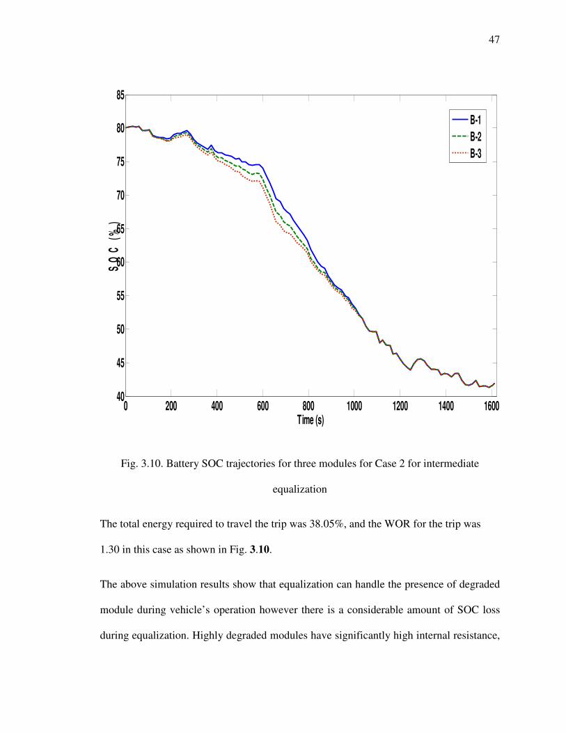
Fig. 3.10. Battery SOC trajectories for three modules for Case 2 for intermediate

equalization

The total energy required to travel the trip was 38.05%, and the WOR for the trip was

1.30 in this case as shown in Fig. 3.10.

The above simulation results show that equalization can handle the presence of degraded

module during vehicle’s operation however there is a considerable amount of SOC loss

during equalization. Highly degraded modules have significantly high internal resistance,

0 200 400 600 800 1000 1200 1400 160040

45

50

55

60

65

70

75

80

85

Time (s)

SO

C (

%)

B-1

B-2

B-3

48

which would waste the battery energy and in turn lead to uneconomical operation. If the

module-specific internal resistance can be identified online, the vehicle owners can

perform the economical analysis based on their preferred trips, and make reasonable

decision on module replacement.

49

4. Simulation Results for Group Performance

In this chapter, we discuss simulation results for cost of charging batteries for a week in

summer and winter months. Also, with the smart grid implemented, we can calculate the

cost discharging energy from the electric vehicles to the grid. We optimize the simulation

scenarios with various battery conditions implemented on the group of electric vehicles

classified based upon their age.

4.1 Driving Cycle

It is well known, that the performance of electric vehicle is stochastic and depends on

many random variables. We have to take into account this random behavior.

0 200 400 600 800 1000 1200 1400 1600-6

-4

-2

0

2

4

6

Time (s)

Acc

eler

ati

on

(m

/sec

2)

(a)

50

Fig. 4.1. Inputs for driving cycle, (a) Acceleration for 100 vehicles for total distance (b)

Velocity for 100 vehicles for total distance

The inputs to the vehicle model are acceleration and velocity for the same trip travelled

from 124 West Freistadt Road in Thiensville to 3200 North Cramer Street in Milwaukee

in Fig. 3.4 with the random behavior for the driving conditions. As the trips are random,

the whole trip is completed with different time segments, but the distance covered by

each trip is the same.

The complete driving cycle includes constant velocity, constant acceleration and constant

deceleration cycles. There are 16 segments which form a complete driving cycle.

0 200 400 600 800 1000 1200 1400 1600 18000

5

10

15

20

25

30

35

40

Time (s)

Vel

oci

ty (

m/s

ec)

(b)

51

We have used same configuration of the electric vehicle as mentioned in Table 3.1.

4.2 Electricity Cost

In the smart grid systems, the cost of electricity varies during the 24 hour period of the

day, and 365 days of the year. We also have the advantage to sell the energy and use the

energy as per our convenience.

0

10

20

30

40

50

60

70

1 2 3 4 5 6 7 8 9 10 11 12 13 14 15 16 17 18 19 20 21 22 23 24

Pri

ce (

$/M

w)

Hours during day

Avg Price

(a)

52

Fig. 4.2. Average energy requirement and cost for a week in summer, (a) Average energy

cost for a week in summer, (b) Average energy requirement for a week in summer.

(www.midwestiso.org)

The average cost of energy and amount of energy on the grid is represented as shown in

Fig. 4.2. We observe the cost of energy during the nights is quite low compared to the

cost of energy during the day time. The cost of energy from 12:00-7:00 AM is very less

compared to the peak hours i.e. from 7:00AM to 7:00PM. There is deviation in the prices

of energy and energy requirements on a daily basis.

0

10000

20000

30000

40000

50000

60000

70000

80000

90000

100000

1 2 3 4 5 6 7 8 9 10 11 12 13 14 15 16 17 18 19 20 21 22 23 24

Act

ual

Lo

ad

(M

W)

Hours during day

Avg Load

(b)

53

0

20

40

60

80

100

120

1 2 3 4 5 6 7 8 9 10 11 12 13 14 15 16 17 18 19 20 21 22 23 24

Pri

ce (

$/M

w)

Hours during day

30-Jul

31-Jul

1-Aug

2-Aug

3-Aug

(a)

54

Fig. 4.3. Daily energy requirement and cost on daily basis for a week in summer, (a)

Energy price per hour on daily basis for a week in summer, (b) Energy requirement for a

week on daily basis in summer

We can clearly observe that there is deviation in the prices of energy on daily basis. The

price of electricity on Monday 30th July 2012 was $95.78 and at the same time on

Tuesday 31st 2012 was $35.09. Thus there is almost $60 difference in 2 consecutive days

for the same hours of energy requirement. This makes it essential to know the correct

times of charging and discharging of electric vehicles so that the operation is cost

0

10000

20000

30000

40000

50000

60000

70000

80000

90000

100000

1 2 3 4 5 6 7 8 9 10 11 12 13 14 15 16 17 18 19 20 21 22 23 24

En

ergy o

n G

rid

(M

Wh

)

Hours during day

30-Jul

31-Jul

1-Aug

2-Aug

3-Aug

(b)

55

efficient. Similarly, data about winter would help us to know the behavior of the energy

on the grid.

0

5

10

15

20

25

30

35

40

45

50

1 2 3 4 5 6 7 8 9 10 11 12 13 14 15 16 17 18 19 20 21 22 23 24

Pri

ce (

$/M

w)

Hours during day

Avg Price

(a)

56

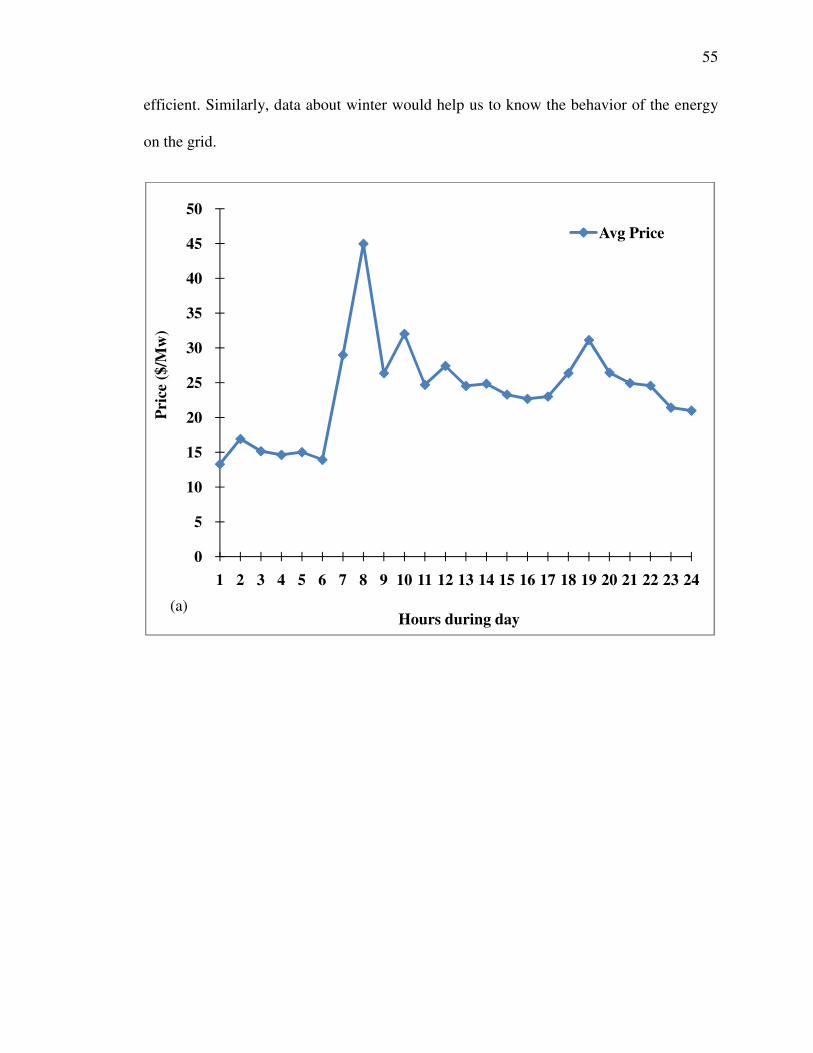
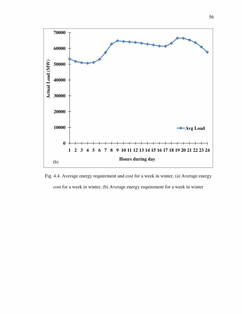
Fig. 4.4. Average energy requirement and cost for a week in winter, (a) Average energy

cost for a week in winter, (b) Average energy requirement for a week in winter

0

10000

20000

30000

40000

50000

60000

70000

1 2 3 4 5 6 7 8 9 10 11 12 13 14 15 16 17 18 19 20 21 22 23 24

Act

ual

Load

(M

W)

Hours during day

Avg Load

(b)

57

Fig. 4.5. (a) Energy price per hour on daily basis for a week in winter, (b) Energy

requirement for a week on daily basis in winter

-20

0

20

40

60

80

100

120

1 2 3 4 5 6 7 8 9 10 11 12 13 14 15 16 17 18 19 20 21 22 23 24

Pri

ce $

/Mw

Hours during day

9-Jan

10-Jan

11-Jan

12-Jan

13-Jan

0

10000

20000

30000

40000

50000

60000

70000

80000

1 2 3 4 5 6 7 8 9 10 11 12 13 14 15 16 17 18 19 20 21 22 23 24

Load

(M

Wh

)

Hours during day

9-Jan

10-Jan

11-Jan

12-Jan

13-Jan

(b)

(a)

58

We can observe in Fig. 4.4 (a) that the average cost for the whole week is in the range

~$10-15. But when we see the cost difference on a daily basis, we see that there are two

hours on Monday 9th Jan 2012 during which the cost is below zero which indicates that

the user earns money for using energy from the grid. The negative cost is due to the cost

associated with the minimum energy on the grid and the variable energy required on the

grid.

The striking difference when we compare Fig. 4.4 and Fig. 4.5 is that the peak hours

when the energy cost is at highest varies with the specific time of the day. During

summers, the highest energy cost is at the end of the day from 3:00-7:00 PM where as the

highest price of energy during winter months at the beginning of the day from 7:00 AM-

12:00 PM.

59

4.3 Battery Charging Configuration

The battery internal resistance rises with its age and the pattern of usage. It does not

increase overnight, but increases gradually on regular usage. There are many factors

which contribute to the rise in the internal resistance like usage over a period of time,

deep discharge cycles, various uncertainties, variable current input and output

requirements etc. The internal resistance values used in this research are approximately

equivalent to the lithium ion batteries of Chevrolet Volt. We assume that the increase in

internal resistance is over the life of the battery.

Table 4.1. Battery internal resistance as per the age of battery during discharging

We assume that the battery life for 6 years in this study that does not imply that the

battery is not usable after 6 years. We just intend to study its performance through its

working life. We assume that batteries are charged from 30% to 80% SOC on a daily

basis. We assume that batteries are at 80% SOC at the beginning of the day i.e. at

7:00AM and it returns to 30% at the end of the day i.e. at 7:00 PM. The battery starts

charging from 7:00 PM and is completely charged by 7:00 AM the next morning.

Name Battery Age (years) Internal Resistance (Ω)

Group 1 0-1.5 0.104

Group 2 1.5-3.0 0.156

Group 3 3.0-4.5 0.313

Group 4 4.5-6.0 0.521

60

The charging times for electric vehicle change with their age. The charging times for

vehicles depends on battery models. We use the battery model mentioned in Fig. 3.1, and

Eq. 3.2 gives the SOC of the battery during charging.

Fig. 4.6. Charging time for batteries in all the groups

We consider that at the beginning of the charging cycle, the battery is at 30% SOC which

is lowest for the operational range and when the battery is fully charged, we have 80%

SOC on the battery for full charged battery.

The charge process from grid for all batteries in the group is shown as in Fig. 4.6. The

charging time increases as the internal resistance of the battery increase. The batteries are

charged with 240V and 30A current for till 60% SOC and then at 120V and 15A. The

0 2 4 6 8 10 1230

35

40

45

50

55

60

65

70

75

80

Time (Hrs)

SO

C (

%)

Group 1

Group 2

Group 3

Group 4

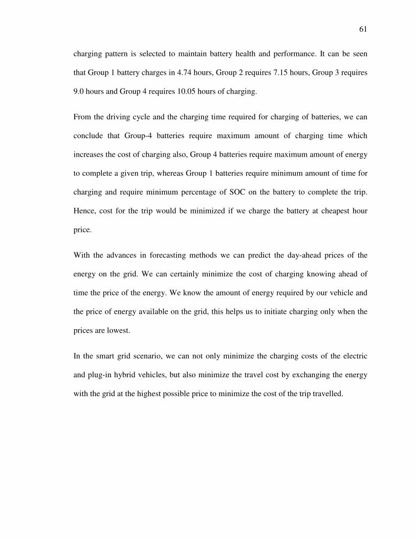
61

charging pattern is selected to maintain battery health and performance. It can be seen

that Group 1 battery charges in 4.74 hours, Group 2 requires 7.15 hours, Group 3 requires

9.0 hours and Group 4 requires 10.05 hours of charging.

From the driving cycle and the charging time required for charging of batteries, we can

conclude that Group-4 batteries require maximum amount of charging time which

increases the cost of charging also, Group 4 batteries require maximum amount of energy

to complete a given trip, whereas Group 1 batteries require minimum amount of time for

charging and require minimum percentage of SOC on the battery to complete the trip.

Hence, cost for the trip would be minimized if we charge the battery at cheapest hour

price.

With the advances in forecasting methods we can predict the day-ahead prices of the

energy on the grid. We can certainly minimize the cost of charging knowing ahead of

time the price of the energy. We know the amount of energy required by our vehicle and

the price of energy available on the grid, this helps us to initiate charging only when the

prices are lowest.

In the smart grid scenario, we can not only minimize the charging costs of the electric

and plug-in hybrid vehicles, but also minimize the travel cost by exchanging the energy

with the grid at the highest possible price to minimize the cost of the trip travelled.

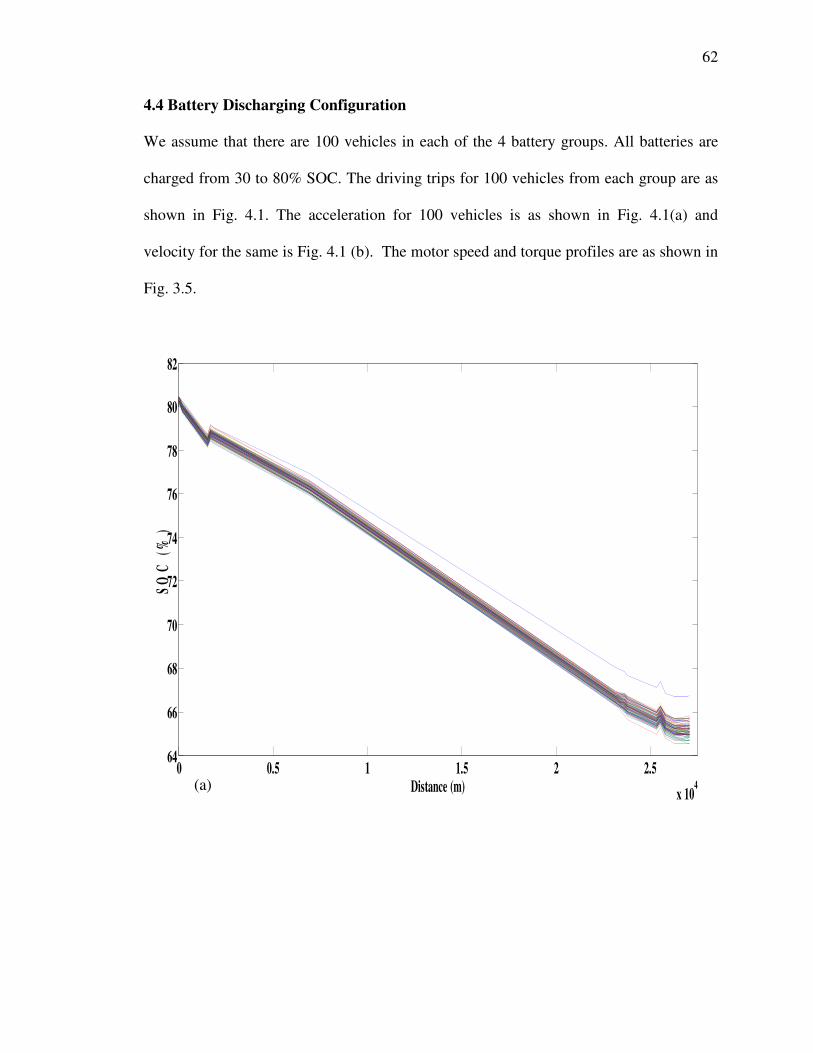
62

4.4 Battery Discharging Configuration

We assume that there are 100 vehicles in each of the 4 battery groups. All batteries are

charged from 30 to 80% SOC. The driving trips for 100 vehicles from each group are as

shown in Fig. 4.1. The acceleration for 100 vehicles is as shown in Fig. 4.1(a) and

velocity for the same is Fig. 4.1 (b). The motor speed and torque profiles are as shown in

Fig. 3.5.

0 0.5 1 1.5 2 2.5

x 104

64

66

68

70

72

74

76

78

80

82

Distance (m)

SO

C (

%)

(a)

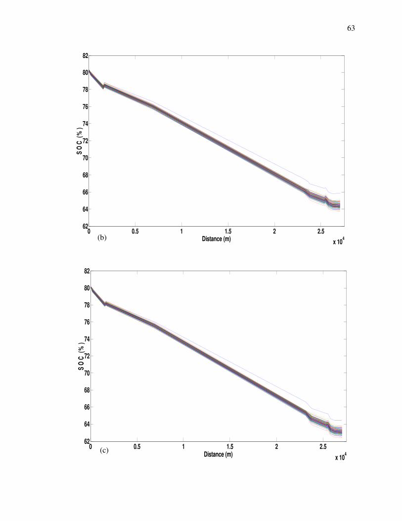
63

0 0.5 1 1.5 2 2.5

x 104

62

64

66

68

70

72

74

76

78

80

82

Distance (m)

SO

C (

%)

0 0.5 1 1.5 2 2.5

x 104

62

64

66

68

70

72

74

76

78

80

82

Distance (m)

SO

C (

%)

(b)

(c)

64

Fig. 4.7. Battery performance: (a) Group 1 batteries, (b) Group 2 batteries, (c) Group 3

batteries, (d) Group 4 batteries

The whole driving cycle is converted into spatial mode as different segments take

different amount of time but the distance remains constant. We drive 100 driving cycles

with 4 battery configurations as mentioned in Table 4.1.

The driving distance for all the batteries is same but the energy required is different as the

battery performance changes with the driving pattern and energy consumed by aged

battery is more. We see that Group-1 batteries require average of 14.79% SOC with a

standard deviation 0.325, Group-2 batteries require average of 15.55% SOC with a

standard deviation of 0.31, Group-3 batteries require average of 16.8% SOC with a

0 0.5 1 1.5 2 2.5

x 104

60

65

70

75

80

85

Distance (m)

SO

C (

%)

(d)

65

standard deviation of 0.31, Group-4 batteries require average of 18.28% SOC with a

standard deviation of 0.34 to complete the trip.

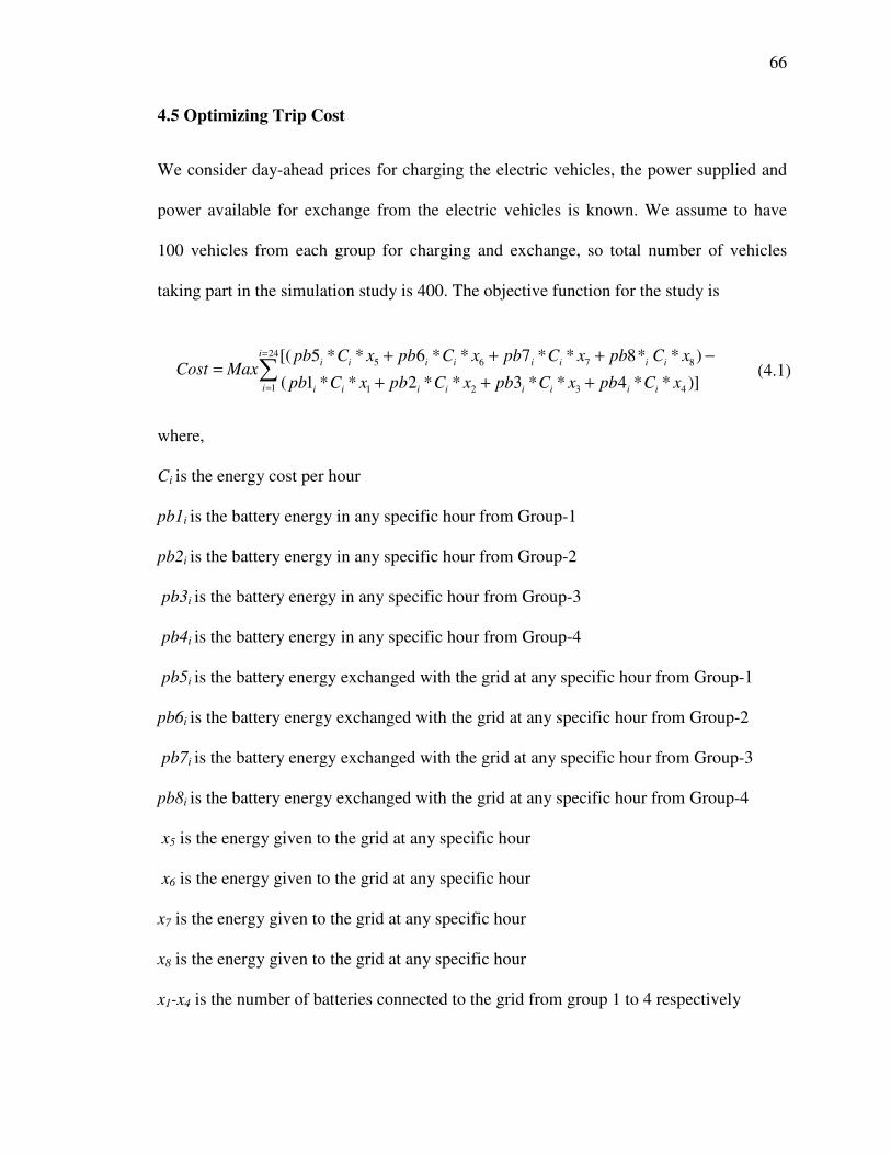
66

4.5 Optimizing Trip Cost

We consider day-ahead prices for charging the electric vehicles, the power supplied and

power available for exchange from the electric vehicles is known. We assume to have

100 vehicles from each group for charging and exchange, so total number of vehicles

taking part in the simulation study is 400. The objective function for the study is

24

5 6 7 8

1 1 2 3 4

[( 5 * * 6 * * 7 * * 8* * )

( 1 * * 2 * * 3 * * 4 * * )]

ii i i i i i i i

i i i i i i i i i

pb C x pb C x pb C x pb C xCost Max

pb C x pb C x pb C x pb C x

=

=

+ + + −=

+ + +∑ (4.1)

where,

Ci is the energy cost per hour

pb1i is the battery energy in any specific hour from Group-1

pb2i is the battery energy in any specific hour from Group-2

pb3i is the battery energy in any specific hour from Group-3

pb4i is the battery energy in any specific hour from Group-4

pb5i is the battery energy exchanged with the grid at any specific hour from Group-1

pb6i is the battery energy exchanged with the grid at any specific hour from Group-2

pb7i is the battery energy exchanged with the grid at any specific hour from Group-3

pb8i is the battery energy exchanged with the grid at any specific hour from Group-4

x5 is the energy given to the grid at any specific hour

x6 is the energy given to the grid at any specific hour

x7 is the energy given to the grid at any specific hour

x8 is the energy given to the grid at any specific hour

x1-x4 is the number of batteries connected to the grid from group 1 to 4 respectively

67

4.6 Opportunity Cost

We assume that we have the knowledge of the cost of charging and cost of discharging

on a specific day of the week. This knowledge provides us the cost of energy on the

specific day for which we estimate the charging discharging pattern. We define

opportunity cost as

($ / )

($ / )

Cost Spent on Charging KWhOpportunity Cost

Cost Earned with Exchanging KWh= (4.2)

To derive the opportunity cost, we require the average cost for charging of batteries from

group 1 to group 4 and money earned with exchanging energy to the grid from group 5 to

group 8 batteries. Batteries from group 1 to group 4 are assumed to have 16.5KWh of on-

board energy when they are completely charged. Batteries from group 5 to group 8 have

varied energy for exchange. Opportunity Cost would be a measure to evaluate the

performance of a particular group of batteries on a specific day for which we forecast the

price of charging and have knowledge of the trip we are planning to travel.

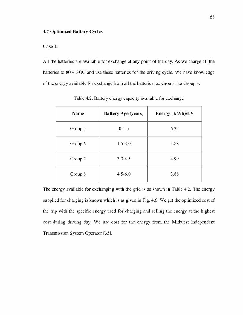
68

4.7 Optimized Battery Cycles

Case 1:

All the batteries are available for exchange at any point of the day. As we charge all the

batteries to 80% SOC and use these batteries for the driving cycle. We have knowledge

of the energy available for exchange from all the batteries i.e. Group 1 to Group 4.

Table 4.2. Battery energy capacity available for exchange

Name Battery Age (years) Energy (KWh)/EV

Group 5 0-1.5 6.25

Group 6 1.5-3.0 5.88

Group 7 3.0-4.5 4.99

Group 8 4.5-6.0 3.88

The energy available for exchanging with the grid is as shown in Table 4.2. The energy

supplied for charging is known which is as given in Fig. 4.6. We get the optimized cost of

the trip with the specific energy used for charging and selling the energy at the highest

cost during driving day. We use cost for the energy from the Midwest Independent

Transmission System Operator [35].

69

Fig. 4.8. Batteries performance connected to grid

We have access to all the batteries for all the hours after charging which results in the trip

cost for 400 vehicles as $195.822.

0

10

20

30

40

50

60

70

80

90

100

1 2 3 4 5 6 7 8 9 10 11 12 13 14 15 16 17 18 19 20 21 22 23 24

No. of

Batt

erie

s fr

om

ever

y g

rou

p

Hours for complete Battery Cycle

Group-1 Group-2 Group-3 Group-4

Group-5 Group-6 Group-7 Group-8

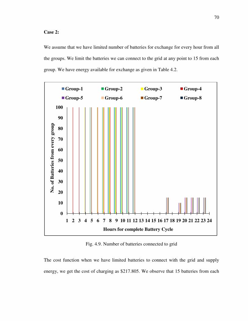
70

Case 2:

We assume that we have limited number of batteries for exchange for every hour from all

the groups. We limit the batteries we can connect to the grid at any point to 15 from each

group. We have energy available for exchange as given in Table 4.2.

Fig. 4.9. Number of batteries connected to grid

The cost function when we have limited batteries to connect with the grid and supply

energy, we get the cost of charging as $217.805. We observe that 15 batteries from each

0

10

20

30

40

50

60

70

80

90

100

1 2 3 4 5 6 7 8 9 10 11 12 13 14 15 16 17 18 19 20 21 22 23 24

No. of

Batt

erie

s fr

om

ever

y g

rou

p

Hours for complete Battery Cycle

Group-1 Group-2 Group-3 Group-4

Group-5 Group-6 Group-7 Group-8

71

group are connected at first 6 highest cost hours and the remaining 10 batteries from each

group are connected at the next highest cost.

Case 3:

In this case we limit the maximum energy, the user can trades with the grid. We assume

that the energy requirement of the grid is maximum 450KWh at any hour of the day. The

data we simulate is for a week in summer i.e. from 7/30/2012 (Monday) to 8/3/2012

(Friday).

0

20

40

60

80

100

120

140

0

10

20

30

40

50

60

70

80

90

100

0 1 2 3 4 5 6 7 8 9 10 11 12 13 14 15 16 17 18 19 20 21 22 23

En

ergy e

xch

an

ged

wit

h g

rid

(K

wh

)

No. of

Ele

ctri

c V

ehic

les

du

rin

g c

harg

ing

Battery Cycle for Electric Vehicle

Group-1 Group-2 Group-3 Group-4

Group-5 Group-6 Group-7 Group-8

(a)

72

0

20

40

60

80

100

120

140

0

10

20

30

40

50

60

70

80

90

100

0 1 2 3 4 5 6 7 8 9 10 11 12 13 14 15 16 17 18 19 20 21 22 23

En

ergy e

xch

an

ged

wit

h g

rid

(K

wh

)

No. of

Ele

ctri

c V

ehic

les

du

rin

g c

harg

ing

Battery Cycle for Electric Vehicle

Group-1 Group-2 Group-3 Group-4

Group-5 Group-6 Group-7 Group-8

(b)

0

20

40

60

80

100

120

140

0

10

20

30

40

50

60

70

80

90

100

0 1 2 3 4 5 6 7 8 9 10 11 12 13 14 15 16 17 18 19 20 21 22 23

En

ergy e

xch

an

ged

wit

h g

rid

(K

wh

)

No. of

Ele

ctri

c V

ehic

les

du

rin

g c

harg

ing

Battery Cycle for Electric Vehicle

Group-1 Group-2 Group-3 Group-4

Group-5 Group-6 Group-7 Group-8

(c)

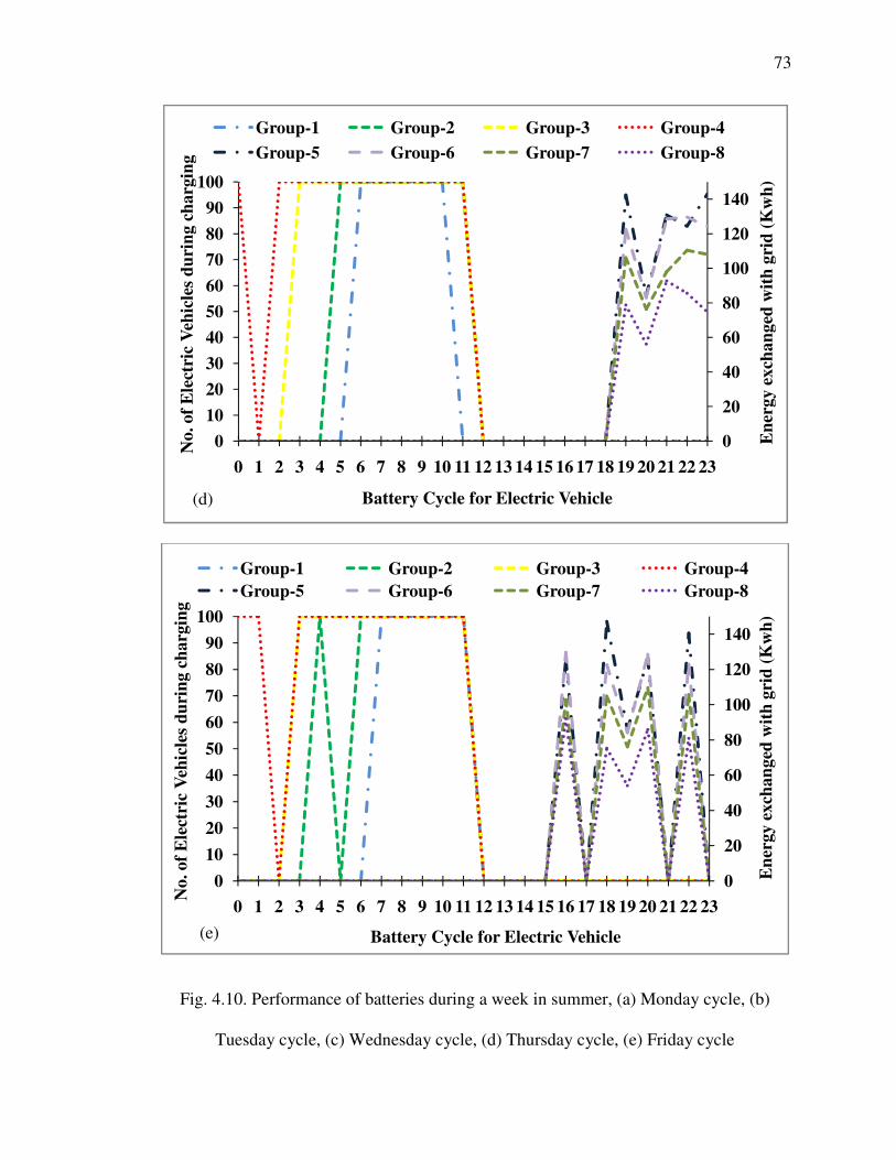
73

Fig. 4.10. Performance of batteries during a week in summer, (a) Monday cycle, (b)

Tuesday cycle, (c) Wednesday cycle, (d) Thursday cycle, (e) Friday cycle

0

20

40

60

80

100

120

140

0

10

20

30

40

50

60

70

80

90

100

0 1 2 3 4 5 6 7 8 9 10 11 12 13 14 15 16 17 18 19 20 21 22 23

En

ergy e

xch

an

ged

wit

h g

rid

(K

wh

)

No. of

Ele

ctri

c V

ehic

les

du

rin

g c

harg

ing

Battery Cycle for Electric Vehicle

Group-1 Group-2 Group-3 Group-4

Group-5 Group-6 Group-7 Group-8

(d)

0

20

40

60

80

100

120

140

0

10

20

30

40

50

60

70

80

90

100

0 1 2 3 4 5 6 7 8 9 10 11 12 13 14 15 16 17 18 19 20 21 22 23

En

ergy e

xch

an

ged

wit

h g

rid

(K

wh

)

No. of

Ele

ctri

c V

ehic

les

du

rin

g c

harg

ing

Battery Cycle for Electric Vehicle

Group-1 Group-2 Group-3 Group-4

Group-5 Group-6 Group-7 Group-8

(e)

74

We use Matlab Linprog function to simulate our data and find the optimized cost of

charging of the batteries of all groups. We study the charging of batteries and discharging

of batteries for a week in summer 2012. We assume that our battery cycle begins 7:00pm

and is completed at 7:00pm the next day. We assume batteries charge from 7:00pm to

7:00am. The batteries are assumed to be at 30% SOC with the beginning of the charging

cycle. Total numbers of batteries which are connected for charging from 7:00pm to

7:00am are represented by group-1 to group-4 in Fig. 4.10. The amount of energy the

batteries exchange with the grid at any hour from 7:00am to 7:00pm is given by group-5

to group-8 in Fig. 4.10.

Table 4.3. Cost of battery cycle per day in summer

Monday Tuesday Wednesday Thursday Friday

Cost Function 149.0338 229.5838 158.1974 246.4039 231.92

The total cost of battery cycle to the user for a weekday is shown as in Table 4.3. We

also know the cost of charging and exchanging energy to the grid.

75

Fig. 4.11. The average performance of batteries in summer

We calculate the total cost of charging batteries from each group-1 to group-4. Then we

also calculate the money earned by exchanging available energy in the batteries with the

grid. Thus we have the estimated costs of energy per kilowatt in charging and discharging

to the grid. The cost for group-1 to group-8 is as shown in Fig. 4.11.

In Fig. 4.11 we can see that group-1 to group-4 is the average performance of batteries

during charging whereas group-5 to group-8 is the average performance to the batteries

0

1

2

3

4

5

6

7

8

9

1 2 3 4 5 6 7 8

Am

ou

nt

in $

/KW

h

No. of Group

Monday Tuesday Wednesday Thursday Friday

76

during exchange. Group-5 consists to batteries from group-1 during exchange, group-6

consist batteries from group-2 during exchange, group-7 consists batteries from group-3

during exchange and group-8 consists batteries from group-8 during exchange.

Table 4.4. Opportunity cost for Week in summer

Monday Tuesday Wednesday Thursday Friday

OCB-1 0.266788 0.657697 0.330647 0.703908 0.544808

OCB-2 0.464569 1.033423 0.512832 1.062479 0.901849

OCB-3 0.699473 1.349427 0.697043 1.364664 1.217155

OCB-4 1.032016 1.710461 0.946929 1.759759 1.607286

We calculate the opportunity cost from equation 18. The opportunity cost indicates the

amount of profit. It is clear from the opportunity cost function that smaller the

opportunity cost, greater is the profit. Opportunity cost greater than 1 indicates that we

spent more on charging the batteries than we earn in exchanging energy to the grid. We

can observe in Table 4.4 that on Monday the opportunity cost for battery-4 is greater than

1 which indicates that the cost or charging the batteries is higher than the cost of energy

exchanged from the batteries to the grid. On Tuesday the opportunity cost for Battery-2,

Battery-3 and Battery-4 is greater than 1, similarly, on Thursday the opportunity cost for

Battery-2 Battery-3 and Battery-4 is greater than 1 and on Friday the opportunity cost for

Battery-3 and Battery-4 are greater than 1. These all cases indicate that the opportunity

cost is greater than 1 and the cost of charging is greater than the money earned from

selling energy from the electric vehicles to the grid. Whereas on Wednesday the

77

opportunity cost of Battery-1, Battery-2, Battery-3 and Battery-4 are less than 1 which

indicates profit from selling the energy to the grid.

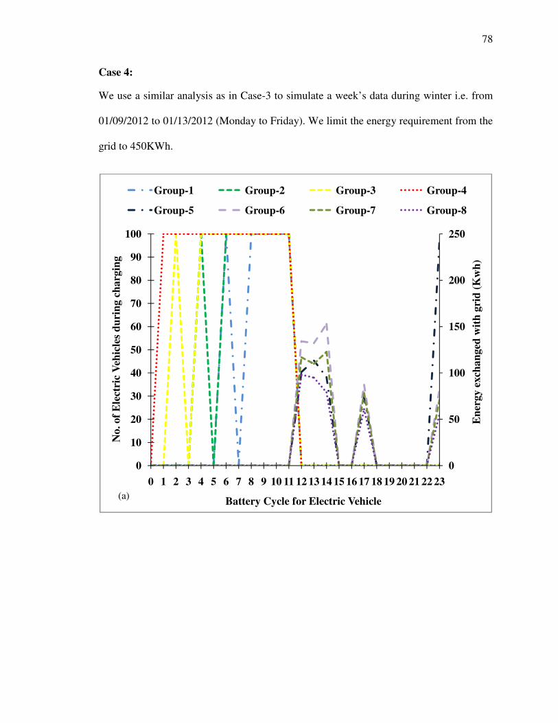
78

Case 4:

We use a similar analysis as in Case-3 to simulate a week’s data during winter i.e. from

01/09/2012 to 01/13/2012 (Monday to Friday). We limit the energy requirement from the

grid to 450KWh.

0

50

100

150

200

250

0

10

20

30

40

50

60

70

80

90

100

0 1 2 3 4 5 6 7 8 9 10 11 12 13 14 15 16 17 18 19 20 21 22 23E

ner

gy e

xch

an

ged

wit

h g

rid

(K

wh

)

No. of

Ele

ctri

c V

ehic

les

du

rin

g c

harg

ing

Battery Cycle for Electric Vehicle

Group-1 Group-2 Group-3 Group-4

Group-5 Group-6 Group-7 Group-8

(a)

79

0

20

40

60

80

100

120

140

160

0

10

20

30

40

50

60

70

80

90

100

0 1 2 3 4 5 6 7 8 9 10 11 12 13 14 15 16 17 18 19 20 21 22 23

En

ergy e

xch

an

ged

wit

h g

rid

(K

wh

)

No. of

Ele

ctri

c V

ehic

les

du

rin

g c

harg

ing

Battery Cycle for Electric Vehicle

Group-1 Group-2 Group-3 Group-4

Group-5 Group-6 Group-7 Group-8

(b)

0

20

40

60

80

100

120

140

160

0

10

20

30

40

50

60

70

80

90

100

0 1 2 3 4 5 6 7 8 9 10 11 12 13 14 15 16 17 18 19 20 21 22 23

En

ergy e

xch

an

ged

wit

h g

rid

(K

wh

)

No. of

Ele

ctri

c V

ehic

les

du

rin

g c

harg

ing

Battery Cycle for Electric Vehicle

Group-1 Group-2 Group-3 Group-4

Group-5 Group-6 Group-7 Group-8

(c)

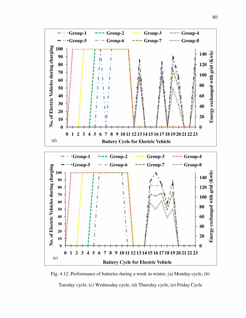
80

Fig. 4.12. Performance of batteries during a week in winter, (a) Monday cycle, (b)

Tuesday cycle, (c) Wednesday cycle, (d) Thursday cycle, (e) Friday Cycle

0

20

40

60

80

100

120

140

0

10

20

30

40

50

60

70

80

90

100

0 1 2 3 4 5 6 7 8 9 10 11 12 13 14 15 16 17 18 19 20 21 22 23

En

ergy e

xch

an

ged

wit

h g

rid

(K

wh

)

No. of

Ele

ctri

c V

ehic

les

du

rin

g c

harg

ing

Battery Cycle for Electric Vehicle

Group-1 Group-2 Group-3 Group-4

Group-5 Group-6 Group-7 Group-8

(d)

0

20

40

60

80

100

120

140

0

10

20

30

40

50

60

70

80

90

100

0 1 2 3 4 5 6 7 8 9 10 11 12 13 14 15 16 17 18 19 20 21 22 23

En

ergy e

xch

an

ged

wit

h g

rid

(K

wh

)

No. of

Ele

ctri

c V

ehic

les

du

rin

g c

harg

ing

Battery Cycle for Electric Vehicle

Group-1 Group-2 Group-3 Group-4

Group-5 Group-6 Group-7 Group-8

(e)

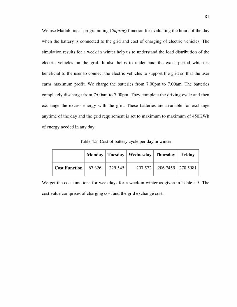
81

We use Matlab linear programming (linprog) function for evaluating the hours of the day

when the battery is connected to the grid and cost of charging of electric vehicles. The

simulation results for a week in winter help us to understand the load distribution of the

electric vehicles on the grid. It also helps to understand the exact period which is

beneficial to the user to connect the electric vehicles to support the grid so that the user

earns maximum profit. We charge the batteries from 7.00pm to 7.00am. The batteries

completely discharge from 7:00am to 7:00pm. They complete the driving cycle and then

exchange the excess energy with the grid. These batteries are available for exchange

anytime of the day and the grid requirement is set to maximum to maximum of 450KWh

of energy needed in any day.

Table 4.5. Cost of battery cycle per day in winter

Monday Tuesday Wednesday Thursday Friday

Cost Function 67.326 229.545 207.572 206.7455 278.5981

We get the cost functions for weekdays for a week in winter as given in Table 4.5. The

cost value comprises of charging cost and the grid exchange cost.

82

Fig. 4.13. Costs incurred and gained during charging and exchanging energy with grid in

winter

From Fig. 4.13, we can estimate the cost of charging from the cost values of group 1 to

group 4 during a week. We know the cost of exchanging energy with the grid from the

cost values of group 5 to group 8. We calculate the opportunity cost as given in equation

6. Group-1 to group-4 is the average performance of batteries during charging per hour

whereas group-5 to group-8 is the average performance to the batteries during exchange

to the grid per hour. Group-5 consists to batteries from group-1 during exchange, group-6

0

1

2

3

4

5

6

7

8

9

1 2 3 4 5 6 7 8

Am

ou

nt

in $

/KW

h

No. of Groups

Monday Tuesday Wednesday Thursday Friday

83

consist batteries from group-2 during exchange, group-7 consists batteries from group-3

during exchange and group-8 consists batteries from group-4 during exchange.

Table 4.6. Opportunity Cost for a week in winter

Monday Tuesday Wednesday Thursday Friday

OCB-1 0.030171 0.690971 0.902569 0.773916 0.763186

OCB-2 0.328167 1.030022 1.407692 1.302486 1.158731

OCB-3 0.79132 1.256656 1.715464 1.822246 1.478382

OCB-4 1.26712 1.506383 2.140395 2.430348 1.802676

Thus from Table 4.4 and Table 4.6, we can clearly observe that there are cases for battery

group’s where we are at a loss charging the batteries to 80% of SOC. We intend to reduce

the cost of charging by charging the batteries only to cater the trip in the cases where loss

is registered. We observe from Table 4.6 that opportunity costs for Battery-1, Battery-2

Battery-3 and Battery-4 is greater than 1 from Tuesday to Friday of the week, whereas

the opportunity cost for Battery-4 is greater than 1. The opportunity costs for batteries

less than 1 indicate profit by exchanging energy from the user to the grid. Our intention is

to reduce the battery cycle cost by reducing the energy level on the battery which

facilitates charging batteries to lower energy level.

84

5. Conclusions and Recommendations

In this study, we proposed a metric to determine the worthiness of replacement (WOR)

for the battery. This idea was successfully demonstrated with two module and three

module systems. We can conclude from the simulation that with drop in SOC and

increase in internal resistance, battery performance decreases during a driving cycle. As

the WOR number increases, the battery tends to be more prone to replacement. Though

we work in acceptable limits of the battery in our simulation study, there is a considerable

loss of energy due to the internal resistance of low energy cell. If a worse battery is

considered for that matter, the battery would run out of energy during a driving cycle and

the trip will be incomplete. Thus with the knowledge of the health map, we could exactly

specify whether the onboard energy can complete the trip successfully. It is completely a

user’s choice to opt for replacement of the poor cell, as the user only has the knowledge

of his trip and the performance of the batteries. We introduce an index so that the user

makes his decision for replacement based the cost of battery, labor and overall utility

requirements.

As the battery performance degrades over its life time, it takes more time for charging.

As the time for charging increases, the charging cost also will increase. The batteries also

use more energy compared to the performance of the batteries when they are new. This

adds on to the cost of driving the trip. With the optimization of the charging and

discharging cycles based on the battery health, we can minimize the cost of trip traveled.

We exploit the smart grid system to balance the energy requirement and provide

advantage to the user of the opportunity for exchange of energy with the grid. The

85

knowledge of the price of energy and the quantity of energy required by the trip enables

us to establish for our pattern of charging and discharging cycles.

Our future research is to consider cases with degraded cells and consider the battery

behavior more rigorously. Also we tend to model the behavior of the internal resistance

with various cases during the driving cycle. We intend to know the state of charge of

batteries based on the internal resistance map. Also, we will aim to judge the charging

patterns for each battery and to limit the state of charge (SOC) of the batteries so as to

minimize the cost of trip and maximize our profit when energy is exchanged with grid.

86

References

1. "Electric car boom - Fiji Times Online". Fijitimes.com. 03-04-2010.

2. Liuchen Chang, “Recent Developments of Electric Vehicles and their Propulsion

Systems”,Aerospace and Electronic Systems Magazine, IEEE, Dec 1993 ,Volume: 8

Issue: 12.

3. Energy Information Administration “Annual Energy” 2009.

4. Whittingham M.S., “Electrical Energy Storage and Intercalation Chemistry”, Science

192 (4244), 1976, pp. 1126-1127.

5. Yoshino Akira, “Secondary Battery”, issued May 1985 assigned to Asahi Kasei.

6. Nazri, Gholamabbas and Pistoia, Gianfranco, “Lithium batteries: science and

Technology”, 2004, Springer ISBN 1402076282.

7. Salameh Z.M., Casacca.M.A. and Lynch W.A.,”Mathematical Model for Lead Acid

Batteries”, IEEE Transactions on Energy Consversion,Vol. 7, No.1, Mar. 1992 pp.

93-98.

8. Valvo M. Wicks F.E., Robertson D. and Rudin S.,”Development and Application of an

Improved equivalent Circuit Model of a Lead Acid Battery ”, Proc. Energy

Conversion Engineering Conference, Vol. 2 Aug 1996, pp. 1159-1163.

9. Ceraolo M., “New Dynamical Models of Lead-Acid Batteries,” IEEE Transactions on

Power Systems, Vol.15 No.4, Nov. 2000, pp. 1184-1190.

10. Buller. S, Thele M., Doncker R.W.D and Karden E.,”Impact Based Simulation

Models of Supercapacitors and Lithium-ion Batteries for Power Electronic

Applications,” Conf. Rec. 2003, Ind. Appl. Conf. Vol.3 pp. 159601600.

87

11. Hageman S.C.,”Simple Spice Models Let You Simulate Common Battery Type,”

EDN,Oct 1993, pp. 17-132

12. Gold S., “A P-Spice Macro-Model for Lithium-ion Batteries, ”Proc.12th Annual

Battery Conference Applications and Advances, 1997, pp.215-222.

13. Vasebi A, Bathaee S.M.T and Partovibakhsh,”Predicting State of Charge of Lead

Acid Batteries for Hybrid Electric Vehicles by Extended Kalman Filter,” Energy

Conversion and Management Vol. 49, 2008, pp.75-82.

14. Cassani P and Williamson S.,”Design,Ttesting and Validation of a Simplified Control

Scheme for a Novel Plug-in Hybrid Electric Vehicle Battery Cell Equalizer, ” IEEE

Transactions on Industrial Electronics Vol. 57. No 12. Dec. 2010.

15. Park H.S., Kim C., Park K, Moon G and Lee J.,”Design of Charge Equalizer Based

on Battery Modularization,” IEEE Transactions on Vehicular Technology, Vol. 58.

No. 7 Sept. 2009.

16. J.G.Lozano, M.I.M Montero,M.A.G. Martinez and E.R. Cadaval,”Electric Vehicle

Battery Charger for Smart Grids,” Electric Power Systems Research, Vol.90, 2012,

pp.18-29.

17. A.Y. Saber and G.K. Venayagamoorthy,”Resource Scheduling Under Uncertainty in

a Smart Grid with Renewables and Plug-in Vehicles,”IEEE Systems Journal, Vol.6,

No.1 2012, pp. 103-109.

18. P.Finn, C.Fitzpatrick and D. Connolly, ”Demand Side Management of Electric Car

Charging: Benefits for Consumer and Grid,” Energy, Vol.42, 2012, pp. 358-363.

88

19. A.S. Masoum, A.A. Siada and S. Islam, “Impact of Uncoordinated and Coordinated

Charging of Plug-in Electric Vehicleson Substation Transformer in Smart Grid with

Charging Stations,” IEEE 978-1-4577-0875-6, 2011.

20. C. Guille and G.Gross, ”A Conceptual Framework for the Vehicle-to-Grid

Implementation,” Energy Policy, Vol.37, 2009, pp.4379-4390.

21 . N. Rotering and M.Ilic,”Optimal Charge Control of Plug-in Hybrid Electric Vehicles

in Deregulated Electricity Markets” IEEE Transactions on Power Systems, Vol.26,

No.3 2011, pp. 1021-1029

22. J. Kiviluoma and P. Meibom, “Methodology for Modelling Plug-in Electric Vehicles

in the Power System and Cost estimates for a System with either Smart or Dumb

Electric Vehicles,” Energy, Vol.36, 2011, pp. 1758-1767.

23. K.C.Nyns, E. Haesen and J. Driesen,”The Impact of Charging Plug-in Hybrid Electric

Vehicles on a Residential Distribution Grid,” IEEE Transactions on Power Systems,

Vol. 25. No. 1, 2010, pp. 371-380.

24. H. Khayyam, H. Ranjbarzadeh and V Marano, ”Intelligent Control of Vehicle to

Grid Power,” Journal of Power Sources, Vol. 201, 2012, pp.1-9.

25. M. Ecker, J. Gerschler, J. Vogel, S. Kabitz, F. Hust, P. Dechent and D. Sauer,

“Development of Lifetime Prediction of Model for Lithium-ion Batteries Based on

Extended Accelerated Aging Test Data, ” Journal of Power Sources, Vol. 215, 2012,

pp. 248-257.

89

26. B. Lunz, Z. Yan, J. Gerscheler and D. Sauer, “Influence of Plug-in Hybrid Electric

Vehicle Charging Strategies on Charging and Battery Degradation Cost,” Energy

Policy, Vol. 46, 2012, pp.511-519.

27. V Pop, Bergveld H J, P H L Notten and P P L Regtien, “State-of-the-art of battery

state-of-charge determination”, Measurement Science and Technology, Volume 16,

No. 12.

28. X. Hu, F. Sun and Y. Zou, “Estimation of State of Charge of a Lithium-Ion Battery

Pack for Electric Vehicles Using an Adaptive Luenberger Observer,” Energies, Vol.

3, pp. 1586-1603, 2010.

29. S. Lee, J.-H. Kim, J.-M. Lee and B.-H. Cho, “State-of-Charge and Capacity

Estimation of Lithium-ion Battery Using a New Open-Circuit Voltage versus State-

of-Charge,” Journal of Power Sources, Vol. 185, pp. 1367-1373, 2008.

30. Y.-S. Lee and G.-T. Cheng, “Quasi-Resonant Zero-Current-Switching Bidirectional

Converter for Battery Equalization Applications,” IEEE Transactions on Power

Electronics, Vol. 21, No. 5, pp. 1213-1223, 2006.

31. T.A. Stuart and W. Zhu, “A Targeted Equalizer for Lithium-ion Battery Packs,” Proc.

5th IEEE Vehicle Power and Propulsion Conference, pp. 207-212, 2009.

32. Y.-S. Lee and M.-W. Cheng, “Intelligent Control Battery Equalization for Series

Connected Lithium-Ion Battery Strings,” IEEE Transactions on Industrial Electronics,

Vol. 21, No. 5, pp. 1213-1223, 2005.

33. M. Dubarry, N. Vuillaume and B.-Y. Liaw, “Origins and Accommodation of Cell

Variations in Lion Battery Pack Modelling,” International Journal of Energy

Research, Vol. 34, No. 2, pp. 216-231, 2009.

90

34. C. Sen and N. C. Kar, “Battery Pack Modeling for the Analysis of Battery

Management System of a Hybrid Electric Vehicle,”Proc. 5th

IEEE Vehicle Power

and Propulsion Conference, pp. 207-212, 2009.

35. www.midwestiso.org

[https://www.midwestiso.org/Library/MarketReports/Pages/MarketReports.aspx]