Embed Size (px)
Citation preview
Effects of Interlaminar Stress Gradients on Free Edge Delamination
in Composite Laminates
A Thesis
Submitted to the Faculty
of
Drexel University
by
Simon Chung
in partial fulfillment of the
requirements for the degree
of
Doctor of Philosophy
July 2003

ii
Dedications
To My Mother and Father

iii
Acknowledgments
There are many to whom I owe the deepest of gratitude for the completion of
this dissertation. First and foremost, I would like to thank my advisor, Dr. Albert
Wang, for his patience and guidance throughout this study. His coaching has allowed
me to view my research beyond academics and applicable to all areas in life. I would
also like to thank my advisory committee members: Dr. F. Ko, Dr. A. Lau, Dr. H. Sosa,
Dr. T. Tan, and Dr. D.Wootton for their participation, time, and helpful suggestions.
I am grateful to my parents for their continued emotional support during my
graduate studies. Thanks to the officers of the Air Force Grant and Dr. Koerner
Fellowship that supported this study.
I would also like to make special acknowledgments to fellow colleagues. To
my lab partner, Chang Yan, who has offered her assistance in various portions of my
research. And, to my dear friend, Mabel Mark, whose support and genuine interest in
my graduate studies has helped me in countless intangible ways.
To all of you, I will always remember.

iv
Table Of Contents
List of Tables ....................................................................................................................viii
List of Figures..................................................................................................................... ix
Abstract..............................................................................................................................xii
CHAPTER 1. INTRODUCTION..................................................................................1
1.1. LAMINATE STRESS ANALYSIS....................................................................5
1.1.1. Interlaminar Free Edge Stress Field .........................................................6
1.1.2. Free Edge Singular Stress Fields ..............................................................9
1.2. DELAMINATION FAILURE MODELS ........................................................11
1.2.1. The Ply Strength Concept.......................................................................11
1.2.2. Interlaminar Ply Strength Concept .........................................................13
1.2.3. The Effective Flaw Concept...................................................................14
1.3. OBJECTIVES AND SCOPE OF RESEARCH................................................15
1.3.1. Objectives ...............................................................................................15
1.3.2. Scope of Presentation.............................................................................16
CHAPTER 2. FULL FIELD STRESS SOLUTION ...................................................22
2.1 THREE-DIMENSIONAL LAMINATE FORMULATION.........................22
2.1.1 The Ply Constitutive Law.......................................................................22
2.1.2 Governing Field Equations .....................................................................24
2.1.3 Boundary Conditions ..............................................................................26
2.2 LOCAL-GLOBAL STRESS MATCHING TECHNIQUE ..............................28

v
2.2.1 Local Analysis ........................................................................................28
2.2.2 Global Analysis and Local-Global Stress Matching ..............................34
2.3 NUMERICAL EXAMPLES.............................................................................37
2.3.1 Singular Stress Solution .........................................................................38
2.3.2 Finite Element Stress Solution ...............................................................39
2.3.3 Matching.................................................................................................40
2.4 DISCUSSION...................................................................................................42
CHAPTER 3. FREE EDGE STRESS GRADIENT ZONES .......................................52
3.1. FREE EDGE STRESS GRADIENT ZONES IN [+θo/90on]s LAMINATES ...53
3.1.1 Singular Points and their Strengths ........................................................53
3.1.2 Stress Concentration Zones and Zone of Dominance Analysis .............55
3.1.3 Poisson’s Ratio Mismatch Effect ..........................................................59
3.1.4 90o Ply Thickness Effect ........................................................................60
3.2. POSSIBLE DELAMINATION LOCATIONS AND FAILURE CONDITIONS.................................................................................................61
3.2.1. Delamination Location and Mode of Failure .........................................62
3.2.2. Delamination Onset Strain .....................................................................64
3.2.3. Transverse Cracking vs. Delamination...................................................65
3.3. DISCUSSION...................................................................................................66
CHAPTER 4. FREE EDGE DELAMINATION ANALYSIS.....................................78
4.1. THE EFFECTIVE FLAW CONCEPT.............................................................79
4.1.1 Effective Interlaminar Flaws ..................................................................79
4.1.2 Fracture Criterion ...................................................................................80
4.1.3 The Range of the Effective Flaw Size ....................................................83

vi
4.2. DELAMINATION INITIATION.....................................................................84
4.2.1 Thermal Effects ......................................................................................86
4.2.2 Poisson’s Ratio Mismatch Effects ..........................................................88
4.2.3 Ply Thickness Effects .............................................................................89
4.3. DELAMINATION GROWTH .........................................................................91
4.4. DISCUSSION...................................................................................................93
CHAPTER 5. MICRO-STRESS FIELD ANALYSIS ...............................................104
5.1 MACRO TO MICRO MODELING ...............................................................105
5.1.1. Fiber/Matrix Microstructure .................................................................105
5.1.2. Representative Volume Element Concept ............................................106
5.1.3. Effective Ply Properties Prediction ......................................................107
5.2 THE MODIFED MULTI-FIBER RVE SCHEME.........................................108
5.3 MICRO-STRESS ANALYSIS .......................................................................110
5.2.1 Finite Element Model...........................................................................112
5.2.2 Micro- Stress Field ...............................................................................113
5.2.3 Fiber/Matrix Interfacial Stresses .........................................................116
5.4 DISCUSSION.................................................................................................118
CHAPTER 6. SUMMARY AND CONCLUSIONS.................................................128
6.1. SUMMARY/CONCLUSIONS.......................................................................128
6.2 DIRECTIONS FOR FUTURE WORK ..........................................................133
List of References ............................................................................................................136
APPENDIX A: NOMENCLATURE...........................................................................142
APPENDIX B: PLY STIFFNESS ROTATION ..........................................................144

vii
APPENDIX C: SINGULAR STRESS SOLUTION ...................................................148
APPENDIX D: CRACK CLOSURE SCHEME.........................................................158
VITA…............................................................................................................................163

viii
List Of Tables
1.1. Tensile strength of T300/934 [0o,45o,90o]s laminates as a function of ply
stacking sequence.................................................................................................18 1.2. Critical tensile stress at onset of delamination for T300/934
[+ 45on / -45o
n/ 0on/ 90o
n]s as a function of ply thickness......................................18 2.1. Material properties for graphite-epoxy composite systems, Case A,
B and C for stress matching method ...................................................................44 2.2. Singularity strength and matching parameters for Case A, B, and C ..................44 3.1. Numerical results of the Poisson's ratio mismatch effect for the
[+θo?/ -θo?/90o]s laminate series under tension .......................................................67 3.2. Numerical and experimental results for ply thickness effects for the
[ +25o/-25o/90on]s laminate series under tension..................................................67
3.3. Observed onset strain for delamination and associated critical conditions
of the [+25o/-25o/90on]s laminate series under axial tension................................68
4.1. Computed values of Cemax and am for the [+θo / -θo /90o]s laminate series,
assuming mid-plane delamination .......................................................................95 4.2. Computed values of Cemax and am for the [+25o?/ -25o?/ 90o
n]s laminate series, assuming mid-plane delamination. ......................................................................95
5.1. Macro and micro-mechanical material properties for a uni-directional ply ......119

ix
List Of Figures 1.1 Cross-sectional micro-photograph of [+25/-25/90½]s T300/934 laminate
under tension. Shown is delamination at the mid-plane ......................................19 1.2. Cross-sectional micro-photograph of [+25/-25/902]s T300/934 laminate
under tension. Shown is transverse cracking in the 90o plies .............................19 1.3. Onset strain for transverse cracking, delamination, and ultimate failure as a
function of 90o ply thickness for T300/934 [+25/-25/90n]s laminate series under tension........................................................................................................20
1.4. Scales of laminate analysis. At left, fiber/matrix recognized at microscopic
level. At right, ply microstructure smeared at macroscopic level........................21 2.1. Schematic of the laminate subjected to uniform axial tension ............................45 2.2. Local geometry and boundary conditions in the local-global method.................45 2.3. Details of the “ring-scheme” in the finite element mesh for local-global
matching...............................................................................................................46 2.4. Interlaminar stress distribution along the 0o/90o interface ( z=2t) for Case C
[0o/90o]s laminate under tension...........................................................................47 2.5. Angular variation match between local and global stress solutions at various
rings (r) for Case A [Matrix/F iber], λ=-0.308 ....................................................48 2.6. Angular variation match between local and global stress solutions at various
rings (r) for Case B [0o/90o]s, λ= -0.0766 ............................................................49 2.7. Angular variation match between local and global stress solutions at
various rings (r) for Case C [0o/90o]s, λ= -0.0344 ...............................................50 2.8. Log of the interlaminar normal stress (σz) plotted against the log of the radial distance (r). Slope of the plot is used to estimate the singularity strength
(λ).........................................................................................................................51 3.1. Strength of edge singularity(s) at θo/-θo and the-θo/90o
n interface in the [+θo/-θo/90o
n]s laminate series ......................................................................................69
x
3.2. Poisson ratio of the grouped [+θo/-θo] plies and the 90on plies in the [+θo/-
θo/90on]s laminates series......................................................................................69
3.3. Interlaminar normal stress plots for [+25o/ -25 o/90o]s laminate under tension...70 3.4. Interlaminar shear stress plots for [+25o/ -25 o/90o]s laminate under tension....71 3.5. Interlaminar normal stress contours for [+θo /-θ o/ 90 o]s laminate series
under tension........................................................................................................72 3.6. Interlaminar normal stress contours for [+25 o/-25 o /90 o
n]s laminate series under tension........................................................................................................75
3.7. Maximum interlaminar normal and axial stress at the mid-plane as a
function of the 90o ply thickness for [+25o/ -25o/ 90on]s laminate under
tension..................................................................................................................77 3.8. Maximum interlaminar normal and axial stress plot at the mid-plane as a
function of θ for [+θo / -θ o / 90 o]s laminate under tension..................................77 4.1. Effective flaw concept .........................................................................................96 4.2. Schematic of the energy release rate as a function of the crack size for free
edge delamination. ...............................................................................................97 4.3. Schematic of the range of the effective flaw size and the corresponding
range of the onset strain for free edge delamination............................................97 4.4. Energy release rate shape functions for mid-plane delamination of the
[+25o/ -25o /90o]s laminate under tension.............................................................98 4.5. Predicted onset strain (with G = Gcr) as a function of crack size for
mid-plane delamination of the [+25o/ -25o /90o]s laminate under tension............98 4.6. Mechanical (Ge), thermal (GT), and mixed (GeT) components of the energy
release rate as a function of temperature for mid-plane delamination in the [+25o/ -25o /90o]s laminate under tension.............................................................99
4.7. Minimum critical strain as a function of. temperature for mid-plane
delamination in the [+25o/ -25o /90o]s laminate under tension............................99 4.8. Mechancial energy release rate shape functions for mid-plane delamination of [+θo/ -θ o/90o]s laminate series under tension ................................................100 4.9. Mechancial energy release rate shape functions for mid-plane delamination of [+25o/-25o/ 90n
o]s laminate series under tension............................................100

xi
4.10. Zone of Dominance (σz> 1psi/µε) stress contour of crack size ‘a’ for
mid-plane delamination of the [+25o/ -25o/90o]s laminate under tension ..........101 4.11. Zone of Dominance (ZOD) and average interlaminar normal stress (σz avg)
as a function of crack length for mid-plane delamination of [+25o/ -25o/90o]s laminate under tension. σz avg. is the average over a 15 fiber diameter area around the crack-tip ...........................................................................................103
5.1. RVE for the [+25o/ -25o/90o]s at the mid-plane..................................................120 5.2. Axial (σx) and interlaminar normal (σz) stress distributions of the macro and
micro- mechanical models along the mid-plane for [+25o/-25o/90o]s under tension................................................................................................................121
5.3. Macro and macro-mechanical FEA models used for the micro-stress
recovery scheme.................................................................................................121 5.4. Interlaminar normal stress profile at the mid-plane for [+25o/-25o/90o]s
laminate under tension.......................................................................................122 5.5. Axial stress profile at the mid-plane for [+25o/-25o/90o]s laminate under
tension................................................................................................................124 5.6. Scaling factor K for the axial and interlaminar normal stresses plotted
along the mid-plane for the [+25o/-25o/90o]s laminate .......................................125 5.7. Transverse displacement profile at the mid-plane across the free edge for
[+25o/-25o/90o]sunder tension ............................................................................125 5.8. Interlaminar shear stress profile at the mid-plane for [+25o/-25o/90o]s
laminate under tension.......................................................................................126 5.9. Schematic of the stress distribution around a fiber in the 90o ply for
the [+25o/-25o/90o]s laminate under tension.......................................................127 6.1. General methodology to study the effects of interlaminar stress gradient
zones on the free edge delamination problem in composite laminates..............135

xii
Abstract
Effects of Interlaminar Stress Gradients on Free Edge Delamination in Composite Laminates
Simon Chung Albert S.D. Wang, Ph.D.
Edge delamination in fiber-reinforced composite laminates has been a
significant structural reliability concern. This particular laminate failure mode is caused
by the high interlaminar stresses concentrated near the free edges. Due to the complex
fiber/matrix microstructure of laminates, an accurate evaluation of these stresses and
determining their exact role in laminate failure has been difficult. Traditional
approaches to this problem have been based on the “effective-ply” theory in which the
plies in the laminate are represented by an elastic homogenized medium. One result of
this theory is the presence of stress singularities at bi-material interfaces near the free
edge. These stress singularities are thought to be possible causes for edge delamination.
In this research, two key issues in the free edge delamination problem are
addressed: 1) to identify the physical sources for delamination, and 2) to establish a
physical criterion for the onset and growth of delamination. For the first issue, a
rigorous numerical stress ana lysis method is devised to accurately determine the full
field stress solution, including the stress singularity. Key lamination parameters known
to influence the delamination are included in the analysis. The analytical results show
that delamination occurs at the largest sized interlaminar stress concentration zone, or
zone of dominance (ZOD). The ZOD is shown to be more sensitive to the lamination
parameters than the edge singularity is.

xiii
For the second issue, the “effective flaw concept” is used to model
delamination within the confines of linear elastic fracture mechanics. In this concept,
an edge flaw is introduced as a starter crack inside the ZOD, and the growth of the flaw
is simulated using finite element methods. Good agreement between the simulated
results and experiments is achieved provided that the effective flaw is sufficiently
large. However, because the crack growth simulation is performed on the “effective-
ply”, justification of the effective flaw at this point is heuristic. An effort is then made
to recover the stress field at the fiber/matrix level near the free edges. Comparisons are
made between the macro and micro-stress fields, in hope to provide a rational
connection to the effective flaw of the macro-analysis.

xiv

1
CHAPTER 1: INTRODUCTION
Fiber-reinforced laminates are one of the basic forms of composite materials.
Laminates are typically manufactured using a number of pre-peg unidirectional plies
bonded together into a layered structure. They are most effective in the form of thin
plates or shells and are used in a wide variety of high-performance applications, such
as military and aerospace structures. The appeal of laminates, in addition to their
superior strength-to-weight and stiffness-to-weight ratios, is in their ability to be
custom-tailored to meet specific performance needs. The ply fiber orientation and ply
stacking sequence in lamination allow the stiffness and strength properties to be
designed directionally dependent in response to the applied load. This gives laminates a
unique advantage over conventional materials.
However, these same design and material parameters can cause laminates to fail
in unusual modes. One major mode of failure is inter-ply debonding, or delamination.
While laminates are primarily designed to withstand in-plane loads, high interlaminar
stresses can develop in regions with abrupt changes in material and/or geometry, such
as at free-edges, holes, cut-outs, etc. The interlaminar stresses in these regions are
highly localized with steep gradients. As a result, delamination may form and
propagate into a large crack. It is well known that a localized delamination can lead to
severe structural weakening as well as reduce structure durability [1-3]. For this reason,
there have been many theoretical and experimental studies on the mechanics of
delamination in composite laminates. However, due to the complex nature of the
delamination mechanisms, the problem continues to attract research interest.

2
The uni-axially loaded laminate coupon is used for both experiment and
analysis in most delamination studies. In the experiment, delamination initiation and
growth can be observed near the laminate free edges, and the conditions for failure are
seen to vary with a number of lamination parameters and loading conditions. Bjeletich,
Crossman, and Warren [4] conducted experiments on symmetrically stacked “quasi-
isotropic” laminates by altering the stacking sequence of 0o, +45o, and 90o plies. They
observed that laminates with certain stacking sequences had a higher tendency to
delaminate. Table 1.1 lists their experimental results for six different stacking
sequences. It is seen that the ultimate tensile strengths vary widely with the stacking
sequence. For instance, the [+45o/0o/90o]s laminate exhibited the lowest ultimate
strength at 63 ksi, and the [90o/+45o/0o]s laminate has the highest at 88 ksi. It was
observed that the former laminate had delaminated in the mid-plane prior to ultimate
failure. The latter did not delaminate at all. In this case, the propagation of the free
edge delamination was believed to be the cause of the lowered tensile strength. Similar
results were noted in several other experiments, e.g., Reifsnider, Henneke, and
Stinchcomb [5], Rodini and Eisenmann [6], and Crossman and Wang [7], just to
mention a few.
Another lamination parameter known to influence edge delamination is the
thickness of the plies. Rodini and Eisenmann [6] demonstrated this effect using a series
of [+45on/0o
n/90on]s graphite-epoxy laminates, with n=1, 2, 3. In this series, the ply
stacking sequence is the same in all the laminates such that delamination is induced
under axial loading; however, the thickness of the plies with the same fiber orientation
is varied with the value of n. Table 1.2 lists the experimentally determined onset stress

3
for delamination for the three laminate cases. Results show the onset stress increased
from 29.7 ksi to 45.4 ksi as n decreases from 3 to 1. Therefore, it was reasoned that
delamination initiation can be accelerated when the thickness of the plies is large;
conversely, initiation can be delayed if the thickness of the plies is small.
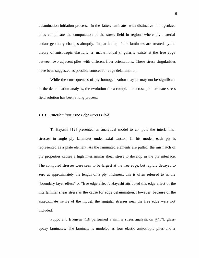
In a later study, Wang and Crossman [7] used a series of [+25o/90on]s graphite
epoxy laminates to investigate the thickness effect of one ply on edge delamination. In
this series, the number of 90o plies is varied from n = ½ to 8, while all other laminate
parameters remained the same. They noted that other cracking modes may occur in the
laminate before, during, and after delamination. Specifically, edge delamination and
90o ply transverse cracking could be induced sequentially or simultaneously depending
on the value of n. For laminates with n = 1/2 or 1, edge delamination was observed as
the first mode of failure. Figure 1.1 shows the cross-sectional view of a delaminated
[+25o/90o1/2]s laminate specimen. Here, delamination formed at the free edge near the
mid-plane and propagated through the 90o ply into the laminate interior. Several
secondary cracks had also formed near the delamination crack tip. However, no
transverse cracking is observed prior to delamination. On the other hand, for laminates
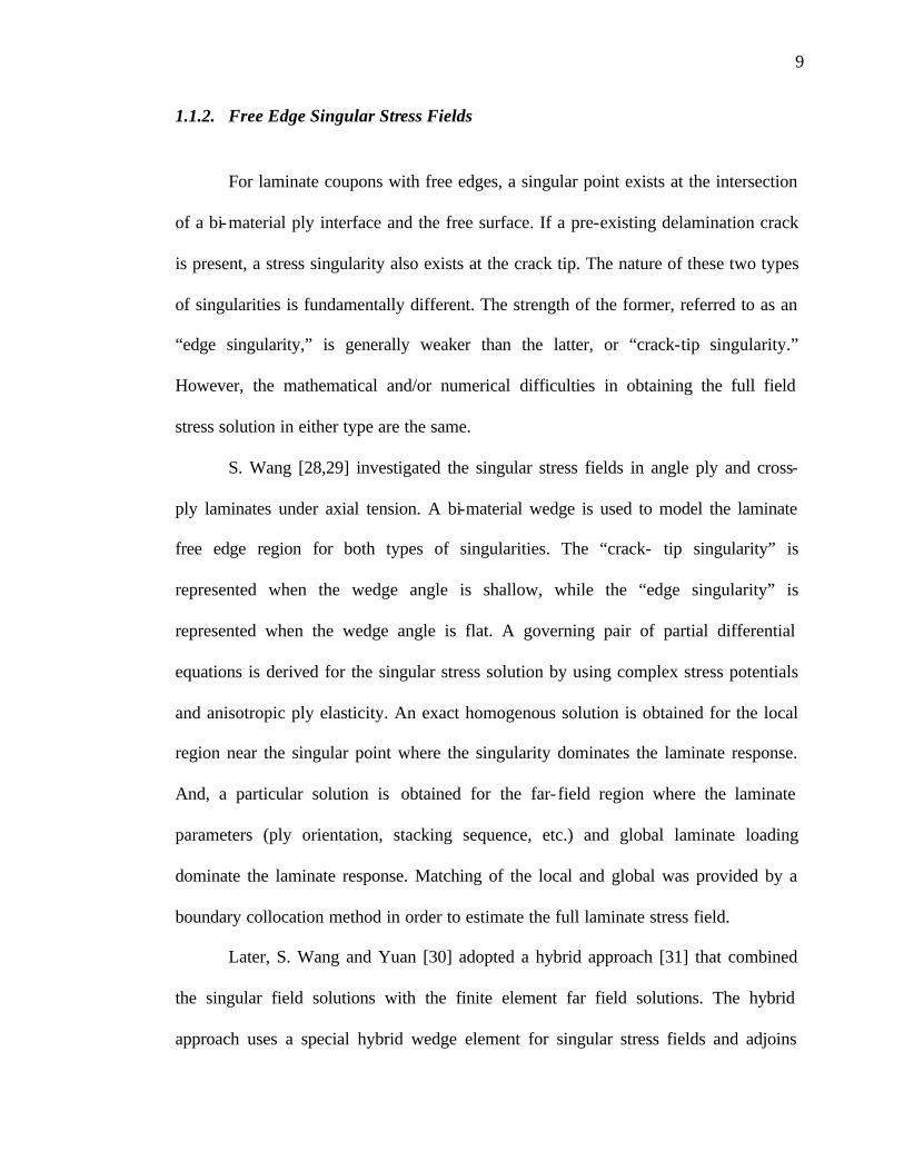
with n> 2, transverse cracking in the 90o ply was observed as the first mode of failure.
Figure 1.2 shows a photomicrograph of the laminate free edge of a [+25o/90o2]s
laminate specimen. Here, transverse cracks formed in the grouped 90o plies prior to
delamination. They are seen to run across the total thickness of the 90o plies, and end at
the -25o/90o interface. Upon further loading, edge delamination was observed to occur
at the tip of the transverse crack at the -25o/90o interface. This suggests an interaction
effect may be present between the two cracking modes.

4
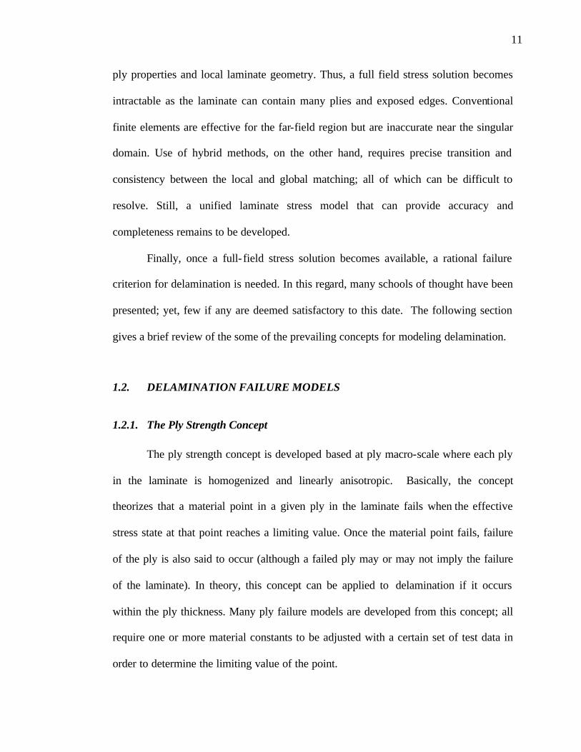
The cracking sequence for the entire [+25o/90on]s laminate series is displayed in
Figure 1.3. The figure shows the onset strains for transverse cracking, delamination,
and ultimate failure plotted against the value of n. It is seen that for n < 2, delamination
is the first mode of failure occurring at the strain of 0.6%; ultimate failure soon follows
after delamination, at 0.65% strain. For n = 2, transverse cracking in the 90o plies
occurs prior to delamination at an applied strain of 0.4%; delamination and ultimate
failure follow upon further loading. However, for n > 2, the onset strains for all three
events reduce rapidly where the onset values for transverse cracking delamination, and
ultimate failure converge.
Clearly, the free edge delamination process can be complicated by the presence
of other failure modes, such as transverse cracking. Even if other damage modes are
not present, the mechanisms of delamination are still influenced by the ply fiber
orientation, ply stacking sequence, ply thickness, and loading conditions. The key to a
proper delamination analysis is to understand the nature of the interlaminar stresses
associated with the various lamination parameters. However, an accurate evaluation of
these stresses so far has proven to be challenging, and a rigorous solution to the
problem is still unavailable. Furthermore, the question remains as how to use the
computed stress field to determine the conditions for when and how delamination
might occur.
In the following sections, some of the prevailing models for computing the
laminate stress field are discussed. In addition, a brief review follows on some of the
failure theories used to predict the onset and growth of delamination. The discussion is

5
focused mainly on the assumptions used and limitations inherent in the analytical
models.
1.1. LAMINATE STRESS ANALYSIS
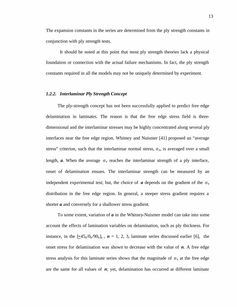
Due to their heterogeneous nature, laminates are generally modeled at two
length scales: microscopic and macroscopic. At the micro-scale, the fibers, matrix,
fiber/matrix interfaces and other quantities of similar sizes in the composite ply are
recognized, as shown in Figure 1.4. However, to compute the full field stresses at this
scale is not only tedious but also impractical due to the numerous material and
geometrical quantities considered.
At the macro-scale, each ply in the laminate is recognized, including the ply- to-
ply interfaces; but, within each ply, the fibers, matrix, and any other microscopic
quantities are smeared to model the ply as a homogenous material. In this way, the ply
becomes the basic building material for the laminate structure. The smearing process is
commonly referred to as the homogenization theory or effective ply theory [8]. It is a
means to compute the effective stress fields for each ply under load. Ply
homogenization has been the basis of most mechanics models for laminates at the
macro-scale, including the widely used classical laminated plate theory [9-11].
However, ply homogenization creates two problems: one is related to the loss
material details at the micro-scale, and the other is related to the macroscopic field
solutions involving mathematical singularities. In the former, loss of the micro-field
details makes it difficult to describe the physical mechanisms that occur inside a ply or
in a ply interface. These mechanisms may be important factor when describing the
6
delamination initiation process. In the latter, laminates with distinctive homogenized
plies complicate the computation of the stress field in regions where ply material
and/or geometry changes abruptly. In particular, if the laminates are treated by the
theory of anisotropic elasticity, a mathematical singularity exists at the free edge
between two adjacent plies with different fiber orientations. These stress singularities
have been suggested as possible sources for edge delamination.
While the consequences of ply homogenization may or may not be significant
in the delamination analysis, the evolution for a complete macroscopic laminate stress
field solution has been a long process.
1.1.1. Interlaminar Free Edge Stress Field
T. Hayashi [12] presented an analytical model to compute the interlaminar
stresses in angle ply laminates under axial tension. In his model, each ply is
represented as a plate element. As the laminated elements are pulled, the mismatch of
ply properties causes a high interlaminar shear stress to develop in the ply interface.
The computed stresses were seen to be largest at the free edge, but rapidly decayed to
zero at approximately the length of a ply thickness; this is often referred to as the
“boundary layer effect” or “free edge effect”. Hayashi attributed this edge effect of the
interlaminar shear stress as the cause for edge delamination. However, because of the
approximate nature of the model, the singular stresses near the free edge were not
included.
Puppo and Evensen [13] performed a similar stress analysis on [+45o]s glass-
epoxy laminates. The laminate is modeled as four elastic anisotropic plies and a

7
separate thin isotropic “shearing” layer is introduced between adjacent plies in order to
account for the shearing action between the +45o plies. The shearing layer, however,
could not take in-plane or interlaminar normal stresses in the laminate.
Pipes and Pagano [14,15] developed a three-dimensional analysis for the free
edge stress field in symmetric laminates under axial tension. Field equations for each
ply are derived based on three-dimensional anisotropic elasticity theory where exact
stress and displacement boundary conditions are imposed on the ply interfaces and the
laminate free edges. The resulting field equations were solved by a finite difference
technique. Their results showed that by altering the laminate stacking sequence and the
fiber orientation of the plies, both interlaminar shear and normal stresses could be
induced near the free edges [16]. The presence of the interlaminar normal stresses was
argued to be as important as the interlaminar shear stresses in causing delamination.
Several other analytical methods subsequently have been developed to
approximate the three dimensional laminate field solutions. For example, Hsu, etc al.
[17], utilized the principle of perturbation for bi-directional laminates. Whitney and
Sun [18] extended a higher order plate theory to account for the interlaminar stresses,
while Tang and Levy [19] employed a boundary layer theory. Pagano [20] latter used a
modified Whitney-Sun theory in which variational principles were incorporated in the
solution.
On the basis of the Pipes-Pagano anisotropic elasticity formulation, Wang and
Crossman [21] developed a quasi three-dimensional finite element method to treat the
free edge problem. Detailed stress solutions of the edge stress field were computed for
laminates of more practical stacking sequences. An accurate three dimensional

8
laminate stress field is provided by using a refined mesh, biased towards the laminate
free edge. In this manner, the finite element solutions successfully accounted for the
highly concentrated interlaminar stresses, particularly the interlaminar normal stress
(σz) near the free edge. In a similar analysis of [+25o/90o]s graphite-epoxy laminates,
Law [22] correlated the presence of high σz at the laminate mid-plane with edge
delamination observed experimentally at the same location [7].
Recently, more advanced finite element schemes have been developed with the
increase in computational power, and have become the preferred method for laminate
stress analysis [23-27]. Murthy and Chamis [26], for example, included super-elements
in their 3-D finite element routine to study laminate free edge effects. Meshing near the
free edge contains a separate element substructure for flexibility and accuracy. Yang
and He [27] employed hexahedronal finite elements in their free edge evaluation of
cross-ply and angle-ply laminates; a conjugate gradient storage scheme is utilized to
overcome problems in storage and computational time.
As seen, accuracy of all the finite element solutions depends on the level of
mesh refinement. Stretched or needled elements could be created in cases where the
mesh refinement are carried to the extreme. Computational time can also be
tremendous in very large finite element schemes. Furthermore, it should be noted that
for laminates containing stress singularities, the conventional finite element methods
may not be capable of providing the true characteristics of the singular region.
Therefore, special treatment may be required to compute the exact stress field at the
singular points; this is discussed in the next section.
9
1.1.2. Free Edge Singular Stress Fields
For laminate coupons with free edges, a singular point exists at the intersection
of a bi-material ply interface and the free surface. If a pre-existing delamination crack
is present, a stress singularity also exists at the crack tip. The nature of these two types
of singularities is fundamentally different. The strength of the former, referred to as an
“edge singularity,” is generally weaker than the latter, or “crack-tip singularity.”
However, the mathematical and/or numerical difficulties in obtaining the full field
stress solution in either type are the same.
S. Wang [28,29] investigated the singular stress fields in angle ply and cross-
ply laminates under axial tension. A bi-material wedge is used to model the laminate
free edge region for both types of singularities. The “crack- tip singularity” is
represented when the wedge angle is shallow, while the “edge singularity” is
represented when the wedge angle is flat. A governing pair of partial differential
equations is derived for the singular stress solution by using complex stress potentials
and anisotropic ply elasticity. An exact homogenous solution is obtained for the local
region near the singular point where the singularity dominates the laminate response.
And, a particular solution is obtained for the far- field region where the laminate
parameters (ply orientation, stacking sequence, etc.) and global laminate loading
dominate the laminate response. Matching of the local and global was provided by a
boundary collocation method in order to estimate the full laminate stress field.
Later, S. Wang and Yuan [30] adopted a hybrid approach [31] that combined
the singular field solutions with the finite element far field solutions. The hybrid
approach uses a special hybrid wedge element for singular stress fields and adjoins

10
with conventional elements for the far field region. Size of the hybrid element depends
on the strength of the singularity, so that smaller hybrid elements are required when
singularity is weak. In such case, matching between the hybrid element and the
conventional elements is difficult to achieve Hence, this approach is shown to be more
effective for the crack tip singularity case than for the edge singularity case.
Bar-Yoseph and Ben-David [32] introduced a transition element in conjunction
with the hybrid finite element approach. The transition element is essentially an
adaptive mesh refinement scheme so that interface conditions between the hybrid
elements near the singular region are compatible with the adjoining conventional
elements. Size of the transition element is estimated based on the average stresses in
the singularity region.
Pagano and Soni [33] proposed a “local-global” variational model where the
laminate thickness is divided into two regions: local region containing the singularity
and the global region for the far field stresses. Variational principles are used to derive
the governing equations for each section; a Reissner variational functional is used in
the local region and a potential energy minimization is used in the global region.
Connection between the local and global solutions is achieved by maintaining
displacement continuity at the local-global interface. If the stress distribution in the
local region is very sharp, the global region needs to be subdivided into two or more
regions in order avoid abrupt transitions between the two regions.
Thus, the pursuit of a complete laminate stress field solution, including stress
singularities, is a continuing research topic [34-37]. The problem is that laminates can
contain multiple singularities where each has its own characteristic, depending on the
11
ply properties and local laminate geometry. Thus, a full field stress solution becomes
intractable as the laminate can contain many plies and exposed edges. Conventional
finite elements are effective for the far-field region but are inaccurate near the singular
domain. Use of hybrid methods, on the other hand, requires precise transition and
consistency between the local and global matching; all of which can be difficult to
resolve. Still, a unified laminate stress model that can provide accuracy and
completeness remains to be developed.
Finally, once a full- field stress solution becomes available, a rational failure
criterion for delamination is needed. In this regard, many schools of thought have been
presented; yet, few if any are deemed satisfactory to this date. The following section
gives a brief review of the some of the prevailing concepts for modeling delamination.
1.2. DELAMINATION FAILURE MODELS
1.2.1. The Ply Strength Concept
The ply strength concept is developed based at ply macro-scale where each ply
in the laminate is homogenized and linearly anisotropic. Basically, the concept
theorizes that a material point in a given ply in the laminate fails when the effective
stress state at that point reaches a limiting value. Once the material point fails, failure
of the ply is also said to occur (although a failed ply may or may not imply the failure
of the laminate). In theory, this concept can be applied to delamination if it occurs
within the ply thickness. Many ply failure models are developed from this concept; all
require one or more material constants to be adjusted with a certain set of test data in
order to determine the limiting value of the point.

12
The maximum stress criterion is one such failure model based on the ply
strength concept. In this model, if one or more of the six stress components at a point in
the ply reaches their respective limiting values, it would imply failure at the point, and
thus also the ply. The limiting stress values are considered the ply strength constants
intrinsic to the ply, which can be determined only by experiment. The maximum stress
concept is applicable mainly when there is only one dominant stress component in the
stress field. The maximum stress criterion remains one of the most widely practiced in
research because of its ease of use.
The maximum strain criterion is another model based on the ply strength
concept. Here, the strain state is considered instead. Failure occurs when any one of
strain components at a point reaches its maximum limiting strain value.
In reality, however, failure in the ply often occurs when none of the stress
components at a point reaches its limiting values. In this case, it is theorized that
interactions among the stresses cause failure. Azzi and Tsai [38] and Hill [39]
presented failure models that include the interaction between the normal and the
shearing stresses in a 2-D ply field; consequently, one disposable constant is added to
the models and the extra constant must be determined by experiment as well. Ply
failure at a point is assumed to occur when a certain combination of these stress
components reaches a limiting value.
Tsai and Wu presented a similar failure model [40] applied to plies with three-
dimensional stress states. In this model, each ply of the laminate is assumed to have a
strength potential; failure at a point is assumed to occur when the potential reaches a
limiting value. The potential is expressed as a power serie s of the stress tensors, σij.
13
The expansion constants in the series are determined from the ply strength constants in
conjunction with ply strength tests.
It should be noted at this point that most ply strength theories lack a physical
foundation or connection with the actual failure mechanisms. In fact, the ply strength
constants required in all the models may not be uniquely determined by experiment.
1.2.2. Interlaminar Ply Strength Concept
The ply-strength concept has not been successfully applied to predict free edge
delamination in laminates. The reason is that the free edge stress field is three-
dimensional and the interlaminar stresses may be highly concentrated along several ply
interfaces near the free edge region. Whitney and Nuismer [41] proposed an “average
stress” criterion, such that the interlaminar normal stress, σz, is averaged over a small
length, a. When the average σz reaches the interlaminar strength of a ply interface,
onset of delamination ensues. The interlaminar strength can be measured by an
independent experimental test; but, the choice of a depends on the gradient of the σz
distribution in the free edge region. In general, a steeper stress gradient requires a
shorter a and conversely for a shallower stress gradient.
To some extent, variation of a in the Whitney-Nuismer model can take into some
account the effects of lamination variables on delamination, such as ply thickness. For
instance, in the [+45n/0n/90n]s , n = 1, 2, 3, laminate series discussed earlier [6], the
onset stress for delamination was shown to decrease with the value of n. A free edge
stress analysis for this laminate series shows that the magnitude of σz at the free edge
are the same for all values of n; yet, delamination has occurred at different laminate

14
stresses. However, the stress gradient of σz near the free edge is shallower if n is large.
In theory, a large a for these laminates can then chosen such that the average of σz is
higher than if n is small. In other words, the size of a can vary with n in order to
consider the ply thickness effects.
Because laminate stress field changes with different laminate configurations,
there is no standard for choosing the size of a. Choice of length is purely empirical,
without physical association to a particular failure mode.
In a recent article, Hinton, etc al. [42] presented a comprehensive review of the
leading strength models, including those for delamination. Over a dozen or more of
such models were investigated along with comparisons between the theoretical
predictions and the experimental observations. Without exception, large gaps existed
between the models and experiments; confidence level is especially poor in the
delamination models. Consequently, to this date, design of laminates against
delamination still relies on experimental data rather than a ply-strength model.
1.2.3. The Effective Flaw Concept
Wang and Crossman [43-44] proposed the “effective-flaw” concept to model
free edge delamination as a crack growth problem. The basis of this concept is that
failure in the laminate, such as localized delamination, originates from the randomly
distributed micro-flaws in the laminate. These flaws are either inherent in the system or
introduced during the manufacturing process. Upon loading, one or more of the micro-
flaws on a certain ply interface may be driven to become a delamination crack
observable at the macro-scale. This defines delamination onset.

15
Since the exact distribution of the micro-flaws is unknown at the macro-scale,
an “effective-flaw” is introduced to represent the collective effects of the micro-flaws
at the macro-scale. The effective flaw is treated as a physical crack so that the fracture
mechanics method can be applied to determine the critical conditions for its growth.
This approach has been shown to capture the effects of most of the lamination variables
effects, including the lamination stacking sequence, ply thickness, fiber orientation, etc.
The outstanding issue in using this concept remains in the details of effective
flaw. The exact size and location of the effective flaw must be known prior to the crack
growth predictions. This issue is yet to be resolved.
1.3. OBJECTIVES AND SCOPE OF RESEARCH
1.3.1. Objectives
The objective of this thesis is to present a series of investigations in response to
two outstanding issues in the free edge delamination problem. This first issue concerns
the role of the interlaminar stresses near the laminate free edges. In this connection, a
method to compute an accurate, full laminate stress field, including stress singularities,
is established. The full- field solution is needed to address correctly the effects of the
lamination parameters and the free edge singularity on the delamination process. Such
assessment is essential in the formation of a proper delamination failure model.
The second issue concerns the critical material conditions governing free edge
delamination onset and growth. For the delamination analysis, models based on the
effective flaw concept are evaluated with the aid of the full- field laminate solution.
Physical associations are sought between the effective flaw and the free edge

16
interlaminar stress field. To determine the actual size of the effective flaw, however, it
is believed that a microscopic analysis of the laminate is needed to account for the roles
of the fibers, matrix, micro-flaws and interactions among them. Here, the macroscopic
full laminate stress field is used in conjunction with a “de-homogenization” process at
the suspected site of delamination. A connection is sought between the macroscopic
laminate stress field and the microscopic field.
1.3.2. Scope of Presentation
With the stated objectives, the [+θo/90o
n]s graphite-epoxy laminate series, with
n = ½ to 3 and θ =0o to 55o under axial tension is used in the free edge delamination
investigation. This laminate series allows control of two key lamination parameters: the
ply fiber orientation (θ) and the 90o ply thickness (n). By varying these two
parameters, changes in the laminate stress field are observed and possible sources that
may influence free edge delamination are identified. This understanding will guide the
development and formulation of a proper delamination criterion.
Chapter 2 presents a local-global stress matching method to compute the full
laminate stress field. The local region is identified as the immediate area near a
singular point located at the laminate free edge. The singular stress solution is then
rendered through ply formulation using complex variable stress potentials and
anisotropic elasticity. The global region is identified as the remainder of the laminate
away from the singularity. Its solution is then rendered by a finite element analysis.
The local and global stress solutions are combined by a stress matching process
between the two solutions; thus, providing a full field solution for the entire laminate.

17
Chapter 3 investigates the effects of the stress singularity and the lamination
parameters, θ and n, that influence the interlaminar stress gradient zones in the
[+θo/90on]s laminate series. In particular, their respective effects are measured in terms
of the magnitudes as well as the size of the stress gradient zone, or zone of dominance
(ZOD), near the free edge. The latter is deemed as a key factor in determining the most
likely location for delamination to occur. It is shown that any criterion for free edge
delamination must take the ZOD into account.
Chapter 4 is focused on evaluating the “effective-flaw” concept in simulating
delamination growth. The basic approach and assumptions of the concept are
discussed. A finite element procedure is used to simulate the delamination process.
Based on an energy criterion, predictions are then made to determine the critical loads
for the onset and growth of delamination. The effects of the lamination variables, such
as the ply orientation, ply-stacking sequence, ply thickness, etc. are investigated on the
energy release rate of the propagating crack.
Chapter 5 presents a multi-scale approach to recover the three-dimensional
micro-stress field at the laminate fiber-matrix scale. A local de-homogenization is near
the laminate free edge where the ZOD is the largest. Force and displacement solutions
from the macro-scale analysis are used as the boundary conditions for the micro-scale
model. The effects of the fiber- fiber interaction in the local stress field are analyzed.
Results show that the local microscopic stresses are complex in the ZOD region. Some
micro-mechanisms are identified as possible sources for delamination onset.
Chapter 6 is a summary of results rendered in this research. Concluding
remarks are made along with suggestions for future work.

18
Table 1.1. Tensile strength of T300/934 [0o,45o,90o]s laminates as a function of ply stackingsequence. [4]
78 ksi[0o/90o/+45o/-45o]s
88 ksi[90o/+45o/-45o/0o]s
77 ksi[90o/0o/+45o/-45o]s
75 ksi[ +45o/-45o/90o/0o]s
72 ksi[0o/+45o/-45o/90o]s
63 ksi[ +45o/-45o/0o/90o]s
Ultimate Tensile StrengthLaminate Stacking Sequence
78 ksi[0o/90o/+45o/-45o]s
88 ksi[90o/+45o/-45o/0o]s
77 ksi[90o/0o/+45o/-45o]s
75 ksi[ +45o/-45o/90o/0o]s
72 ksi[0o/+45o/-45o/90o]s
63 ksi[ +45o/-45o/0o/90o]s
Ultimate Tensile StrengthLaminate Stacking Sequence
29.7 ksin=3
38.1 ksin=2
45.4 ksin=1
Axial Stress at DelaminationOnset
Laminate Series :[+ 45n/0n/90n]s
29.7 ksin=3
38.1 ksin=2
45.4 ksin=1
Axial Stress at DelaminationOnset
Laminate Series :[+ 45n/0n/90n]s
Table 1.2. Critical tensile stress at onset of delamination for T300/934 [+ 45on/-45o
n/0on/90o
n]sas a function of ply thickness. [6]

19
Figure 1.2. Cross-sectional micro-photograph of [+25/-25/902]s T300/934 laminate under tension. Shown is transverse cracking in the 90o plies. [7]
Figure 1.1. Cross-sectional micro-photograph of [+25/-25/90½]s T300/934 laminate under tension. Shown is delamination at the mid-plane. [7]
+25o -25o 90o 90o 90o 90o -25o +25o
mid-planetransverse crack
+25o -25o 90o 90o 90o 90o -25o +25o
mid-planetransverse crack
+25o
- 25o
90o
- 25o
+25o
mid -plane
delamination
+25o
- 25o
90o
- 25o
+25o
mid -plane
delamination

20
Figure 1.3. Onset strain for transverse cracking, delamination, and ultimate failure asa function of 90o ply thickness for T300/934 [+25/-25/90n]s laminate series under tension. [7]

21
Figure 1.4. Scales of laminate analysis. At left, fiber/matrix recognized at microscopic level.At right, ply microstructure smeared at macroscopic level.
..................... . . . .. . . . ...................... . . . .. . . . ........
..... Ply 1
Ply 2
Ply 1
Ply 2
Interlaminar stress
edgesingularity
Microscopic scalePly Homogenization
Macroscopic scale
..................... . . . .. . . . ...................... . . . .. . . . ........
..... Ply 1
Ply 2
Ply 1
Ply 2
Interlaminar stress
edgesingularity
Microscopic scalePly Homogenization
Macroscopic scale

22
CHAPTER 2: FULL FIELD STRESS SOLUTION
The purpose of this chapter is to outline a rigorous, analytical method for
obtaining the complete three-dimensional stress field in composite laminates. Emphasis
is placed near the laminate free-edges, where stress singularities are present.
The laminate analysis is formulated based on the theory of anisotropic elasticity
[45]. For specific results but without the loss of generality, the following
specializations are imposed in the laminate analysis. First, material properties of each
ply are homogenous and linearly elastic using the ply homogenization theory. Second,
the ply stacking sequence is symmetric with respect to the laminate mid-plane. Third,
the laminate has a finite width, and its length is long. Finally, some general
assumptions are made about the laminate, such as no material failure occurs during
loading, no voids or cracks exists in the laminate, and ply-to-ply interfaces are
perfectly bonded and are straight. Figure 2.1 shows a schematic of the laminate model
with the conditions specified above.
2.1 THREE-DIMENSIONAL LAMINATE FORMULATION
2.1.1 The Ply Constitutive Law
The stress-strain relations for the homogenized uni-directional ply in the
principal material directions (L ,t, z) are given by Eq. (2.1) [46]. In this case, the
principal material directions in a ply are defined as L in the longitudinal fiber direction,
t transverse to the fiber direction, and z normal to the ply plane.

23
(2.1)
In Eq. (2.1), the superscript p denotes the principle coordinate system and the
subscripts (1,2,3) corresponds to (L, t, z) system respectively. The material constants,
CijP, are related to the more familiar engineering constants, as given by:
C11p = (1 - v23v32) ∆ E11 C23
p = (v32 – v12v31) ∆ E22
C22p = (1 - v13v31) ∆ E22 C44
p = G23
C33p = (1 – v12v21) ∆ E33 C55
p = G31 (2.2) C12
p = (v21 - v23v31) ∆ E11 C66p = G12
C13p = (v31 - v21v32) ∆ E11
where
∆ = (1 – v12v21 - v23v32 – v13v31 - 2 v12v23v31)-1
Let the global coordinate system (x,y,z) be used for the laminate (see Figure
2.1). For any ply whose fibers are not aligned with the laminate’s x-direction, the
stress-strain relations can be obtained for a special rotation about the z-axis:
τ12p
τ13p
τ23p
σ3p
σ2p
σ1p
C66p 0 0 0 0 0
0 C55p 0 0 0 0
0 0 C44p 0 0 0
0 0 0 C33p C23
p C13p
0 0 0 C23p C22
p C12p
0 0 0 C13p C12
p C11p
=
γ12p
γ13p
γ23p
ε3p
ε2p
ε1p

24
τxy
τxz
τyz
σz
σy
σx
C66 0 0 C36
C26 C16
0 C55 C45
0 0 0
0 C45 C44
0 0 0
C36 0 0 C33
C23 C13
C26 0 0 C23
C22 C12
C16 0 0 C13
C12 C11
=
γxy
γxz
γyz
εz
εy
εx
(2.3)
In Eq. (2.3), the material constants Cij are related to Cij
p in Eq. (2.1) from the ply
transformation law. Details of this transformation are provided in Appendix B.
2.1.2 Governing Field Equations
For a long, finite-width, symmetrically stacked laminate subjected to axial
tension, the laminate cross-section is under generalized plane strain conditions. The
displacement field for this laminate can then be written as [14]:
u = εo x + U(y,z) v = V(y,z) w = W(y,z) (2.4)
where ε o is the applied laminate strain and u, v, and w are the displacements in the x, y,
z directions, respectively. Note that the loading of the laminate, ε o, is specified only in
u, and the displacement functions U, V, and W are independent of x. The strain field is
then derived from the displacement field in Eq. (2.4):
εx = εo εy= V,y εz = W,z
γyz = V,z + W,y γxz = U,z γxy = U,y (2.5)

25
∂ 2 εy ∂ 2 z + ,
∂2 εz
∂2 y ∂2 γyz ∂ y ∂z =
∂γxy ∂z
∂ γxz ∂ y =
Owing to the generalized plain strain condition, the stress-equilibrium equations take
on the reduced form:
τxy,y + τxz,z = 0 σy,y + τyz,z = 0 τyz,y + σz,z = 0 (2.6)
And, the corresponding compatibility equations are:
(2.7)
Substituting the strain-displacement relations, Eq. (2.5), into the stress-strain relation,
Eq. (2.3), and then subsequently into the stress-equilibrium differential equations, Eq.
(2.6), the displacement-equilibrium equations may be written as:
C66U,yy + C55U,zz + C26V,yy + C45V,zz + (C36 + C45)W,yz =0
C26U,yy + C45U,zz + C22W,yy + C44V,zz + (C23 + C44)W,yz =0 (2.8)
(C45 + C36)U,yz + (C44 + C23)V,yz + C44W,yy + C33W,zz =0
Above are the governing field equations for a generic point in the laminate. In theory,
the exact stress field for each ply in the laminate can be found by integrating Eq. (2.8)
over the entire domain of the ply and satisfying the appropriate boundary conditions.
26
2.1.3 Boundary Conditions
For the laminate considered, the top and bottom surfaces of the laminate, as
well as the free edges, are stress free. Also, since the ply-to-ply interfaces are assumed
perfectly bonded, the interlaminar stresses and displacements are continuous across the
ply interfaces:
Traction free surfaces along the upper and lower surfaces of the laminate:
τyz = 0 τxz = 0 σz = 0 (2.9)
Traction free surfaces along the stress free edges:
τxy = 0 τyz= 0 σy = 0 (2.10)
Interface continuity conditions:
ui+1 – ui = 0 σy i+1 – σyi = 0
vi+1 – vi = 0 τxz i+1 – τxzi = 0 (2.11)
wi+1 – wi = 0 τyz i+1 – τyzi = 0
where the superscripts i denote the ith ply in the laminate sequence.
It is noted that the field equations, Eq. (2.8), and the boundary conditions, Eq.
(2.9) to Eq. (2.11), are exact within the premise of linear 3-D elasticity. They are
appropriate for the laminate considered, except at the point of a singularity. Edge
singularities exist at the location where the ply interface of dissimilar materials
intersects the laminate free edge. At any of the singular points, the field solution must
simultaneously satisfy two mutually exclusive conditions: (1) on the free-edge, the
shear stress τyz must be zero, and (2) on the interface, τyz must a finite value. Thus, this
contradiction in the specified boundary conditions causes the localized stress
singularity at the free edge.
27
In an effort to obtain an accurate and complete laminate stress field with edge
singularities, a local-global stress-matching technique is adopted. This technique has
been successful in solving elasticity problems involving singular stress fields, such as
the crack-tip problem along a bi-material interface and the fiber pull-out problem in
composites [47]. There are three major steps in this method: local analysis, global
analysis, and stress matching. The local analysis is formulated for the localized domain
where the singular stresses govern the laminate stress field. The exact singular stress
solution is obtained using Lekhnitskii’s complex variable stress potential theory
followed by an eigenvalue expansion procedure. By defining the local boundary
conditions at the laminate free edge and ply interface matching conditions, this step can
determine the power of the singularity as well as the special (or angular variation) that
is valid to all types of applied loadings and remote constraints. The solution to singular
stress field is computed to within a scaling factor that is determined by the global
response of the laminate. In the global analysis, a 3D finite element scheme is
employed to obtain the overall stress field of the laminate. Near the free edge
singularity point, the finite element mesh is refined and arranged specifically to capture
the angular variation of the stresses. A small but finite region exists in which the stress
solutions of the local and global analysis meet. A perfect match is meet when angular
variations between the two solutions are ident ical. Once matched, a scaling factor can
be computed for the local stresses to maintain consistency with the specified applied
loading and boundary constraints. The final step in this method then combines both
local and global analyses to provide a full- field stress solution.

28
In the next section, detailed formulation for each of the three steps in the stress-
matching method is presented. Several numerical examples are given to illustrate the
methodology. The complete laminate stress field, including the singular stresses at the
laminated edges, is obtained and evaluated.
2.2 LOCAL-GLOBAL STRESS MATCHING TECHNIQUE
2.2.1 Local Analysis
In the local analysis of the laminate, only the immediate region near the free
edge singularity is considered. Figure 2.2 shows the local geometry and local
coordinate system [r, θ, z] of the laminate free edge region as a bi-material half-space.
The upper quarter space, α, and lower quarter space, β , represents two adjacent plies in
the laminate. Note that the region contains only one singular point at the intersection of
the bi-material interface and the free edge.
This configuration is similar to the classical elastic wedge problem, originally
investigated by Bogy [48], and Hein and Erdogan [49]. If the wedge angle is shallow,
then the configuration represents a crack problem; if flat, then it represents a free edge
problem, such as the case considered here. For the wedge problem, the local stress field
is a product of a radial power function and an angular variation:
σij ∼ rλ σ?ij(θ) (for i,j= 1,2,3) (2.12)
where λ is the strength of the singularity, and σ ij(θ) is the spatial or angular variation.

29
b7 ∂6
∂x6 + b6 ∂6
∂x ∂y5
+
A solution technique to the anisotropic elastic bi-material wedge problem had
been presented by Lekhnitskii [45], and later applied to the composite laminate by
S.Wang [28,29]. The technique uses Airy stress functions in terms of two complex
stress potentials U and F to satisfy the governing field equations in Eq. (2.8). Let
U(y,z) and F(y,z) be defined such that the equilibrium equations Eq. (2.6) are
automatically satisfied for each ply, α and β:
σy = ∂ 2U/ ∂z2 τxy = ∂ F/ ∂z
σz = ∂ 2U/ ∂y2 τxz = - ∂ F/ ∂y (2.13)
τyz = - ∂ 2U/ ∂y ∂z
The axial stress component, σx, also exists but is a function of all the stress components
in Eq. (2.13) due to the generalized plain strain conditions.
Substituting the Eq. (2.13) into the stress-strain relations Eq. (2.3) and then the
compatibility equations Eq. (2.7) yield a set of the differential equations in terms of the
functions U and F:
L(U) = 0 and L (F) = 0 (2.14)
Here, L is a six order differential operator:
(2.15)
where
b1 = a33a44 – a34
b2 = 2a34(a36 + a45) – 2a13a66 – 2a45a33
b1 ∂6
∂x6 + b2 ∂6
∂x5 ∂y + b3 ∂6
∂x4 ∂y2 b4 ∂6
∂x3 ∂y3 + b5 ∂6
∂x2 ∂y4 L = +

30
∂
∂y µk Dk = − ∂
∂x
b3 = a33a66 + 4a46a35 – a44(2a23 + a55) – (a36 + a45)2 – 2a34(a24 + a56)
b4 = 2a26a34 + 2(a36 + a45) (a24 + a56) – 2a35 a66 – 2a25 a44 – 2a46(2a23 + a55)
b5 = a22a44 + 4a25a46 + a66(2a23 + a55) – (a24 + a56)2 + 2a26(a36 + a56)
b6 = 2a26(a24 + a56) – 2a46a22 – 2a25a66
b7 = a22a66 – a262
aij =Sij – Si1Sj1/S11 (for i,j = 2...6)
and Sij are the compliance of the ply material equal to [Cij]-1.
The sixth order operator L can be decomposed into six linear operators of the
first order. Eq. (2.14) can then be written as:
D6D5D4D3D2D1(U) = 0 and D6D5D4D3D2D1(F) = 0 (2.16)
where
And the quantities µk are the roots of the characteristic equation:
l11(µ) l 22(µ) −{l12(µ)}2 = 0 (2.17)
where
l11 = a22µ4 − 2 a24µ3 +(2 a23+a44) µ2 − 2a34µ + a33
l22 = a66µ2 − 2 a56µ + a55
l12 = a26µ3 − (a25+a46) µ2 + (a36+a45) µ − a35
To separate the stress field into the radial and angular components, the complex
variable, z= x + µ y, is introduced in Eq. (2.16). A general solution for Eq. (2.16) is
proposed by Lekhnitskii [45]. The solution has the form:
(for k = 1..6)
31
U = Φk (zk) and F = ηΦk’(zk) S
6
S k=1
6
S k=1
6
S 6
k=1
S k=1
6
S k=1
6
S k=1
6
k=1
S k=1
6
(2.18)
where
η = − l11 / l12 = − l12 / l22
and the superscript (’) denotes differentiation of the function Φk with respect to z.
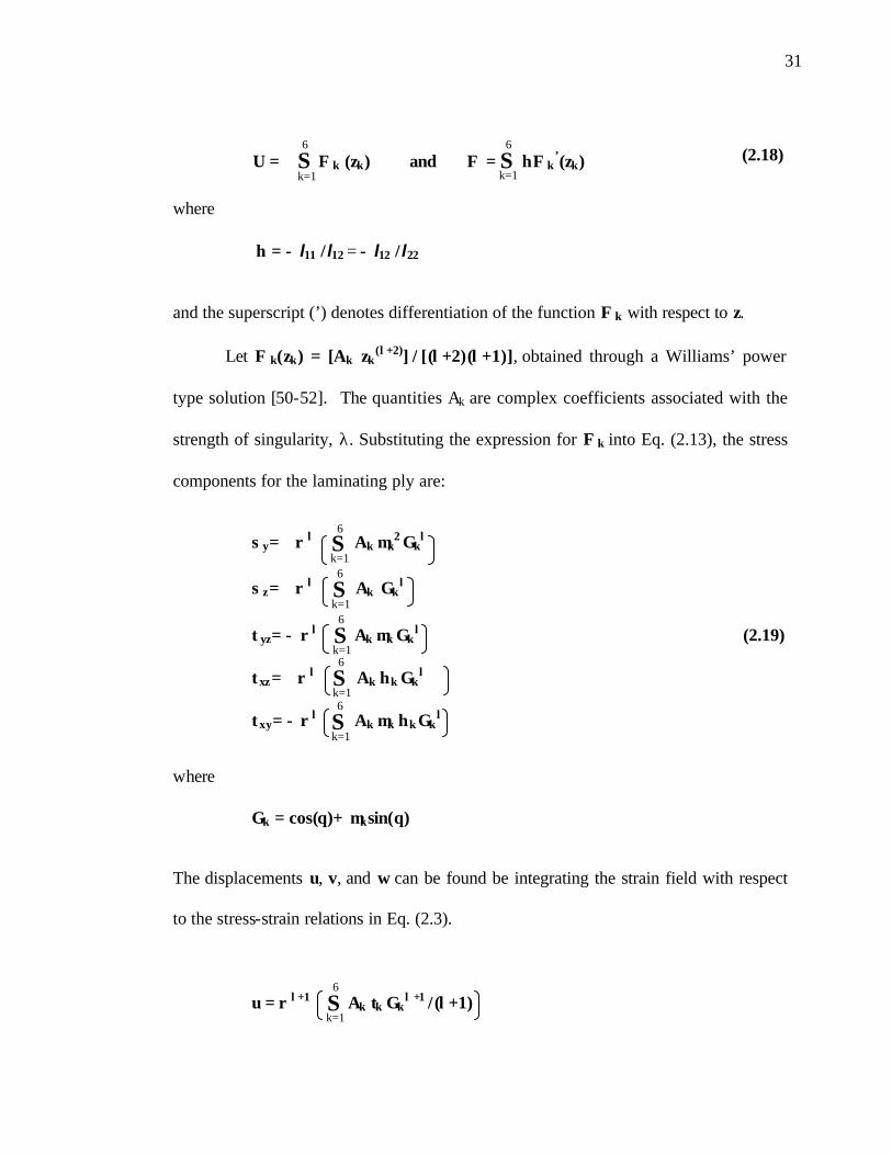
Let Φ k(zk) = [Ak zk(λ+2)] / [(λ+2)(λ+1)], obtained through a Williams’ power
type solution [50-52]. The quantities Ak are complex coefficients associated with the
strength of singularity, λ. Substituting the expression for Φk into Eq. (2.13), the stress
components for the laminating ply are:
σy= r λ Ak µk
2 Γkλ
σz= r λ Ak Γkλ
τyz= - r λ Ak µk Γk
λ (2.19)
τxz= r λ Ak ηk Γkλ
τxy= - r λ Ak µk ηk Γk
λ
where
Γk = cos(θ)+ µksin(θ)
The displacements u, v, and w can be found be integrating the strain field with respect
to the stress-strain relations in Eq. (2.3).
u = r λ+1 Ak tk Γkλ +1 /(λ+1)

32
S k=1
6
S k=1
6
v = r λ+1 Ak pk Γk λ +1 /(λ+1) (2.20)
w = r λ+1 Ak qk Γkλ +1
/(λ+1)
where pk = a22µk
2 + a23 + a25 ηkµk + a24µk
qk = a23µk + a33 /µk + a35 ηk/µk + a36 ηk – a34
tk = a25µk + a35 /µk + a55 ηk//µk + a56 ηk – a45
Note that the stresses Eq. (2.19) are expressed in a separable [r,θ] form; namely, it has
a power type component of the singularity (rλ) multiplied by the angular variation
component (σ?i j(θ)). To compute the stress and displacement fields in Eq. (2.19) and
(2.20), the local boundary conditions have to be specified. The boundary conditions
near the free edge are:
Traction free boundary conditions at the free edge of the half-space:
at θ = +π/2, σy α = τxy
α = τyz α =0
at θ = −π/2 , σy β = τxy
β = τyz β =0 (2.21a)
and,
Interface continuity conditions:
at θ =0 , [σz α, τxz
α, τyz α] = [σz
β, τxzβ, τyz
β]
[u α, v α, w α] = [uβ v β, wβ] (2.21b)

33
Substitution of the boundary conditions in Eq. (2.21) into the stress and displacement
relations in Eq. (2.19) and (2.20) yields a set of twelve algebraic equations. These
equations can be expressed in the matrix form:
[D(λ)] X = 0 (2.22)
The above equation is a standard eigenvalue problem in which λ is the eigenvalue and
X is the eigenvector. X is composed of the complex coefficients [A1α, A2
α, A3α, A4
α ,
A5α, A6
α, A1β, A2
β A3β, A4
β, A5β, A6
β] T.
For a nontrivial solution of X, determinant [D] must vanish and λ can be
obtained:
det [D(λ)] = 0 (2.23)
Eq. (2.23) is a highly transcendental equation. Many values of λ exist and some
are complex. These values can be determined numerically using a standard mathematic
software package (see details in numerical example, Sect. 2.4.1 and Appendix C). The
range of λ is restricted to -0.5 <Re(λ) <0 due to the constraint of finite strain energy.
Re(λ) = -0.5 is the case when a crack exists between the α and β interface, and the
Re(λ) = 0 is the case when α and β are the same material and no singularity is present.
If multiple values of λ exist within this range, then the smallest λ value (most negative)
gives rise to the most dominate singular stresses in the local stress field.
Once the eigenvalue (s) of λ satisfying Eq. (2.23) are found, the coefficients Ak
in X can be computed for each λ. However, the matrix [D] in Eq. (2.22) is rank

34
deficient, where not all the coefficients Ak in X can be determined uniquely. Here, [D]
has a rank of 11 for the 12x12 matrix and one of the coefficients needs to be set
arbitrarily. This arbitrary constant is considered as an amplitude or scaling factor of the
local stress field, whose value that depends upon the global loading conditions. For the
problem considered here, the first coefficient in the eigenvector X, A1α , is set to unity
and the remaining eleven coefficients are then computed. Details of the matrix [D] and
the procedure to solve Eq. (2.22) are given in Appendix C.
After λ and the coefficients Ak in X are determined within a scaling factor, the
angular variations, σ?i j(θ), in the local stress field in Eq. (2.12) can be computed using
Eq. (2.19). σ?i j(θ) is dependent only on the material properties and local boundary
conditions, but is independent of the global applied loading. Hence, the general form of
the local stress field can be represented as:
σij = K r λ σ?i j(θ) (2.24)
where K is the local scaling factor. K can be determined by matching the local stress
field with the global stress field via a local-global stress matching.
2.2.2 Global Analysis and Local-Global Stress Matching While the strength of the singularity, λ, and the angular variation, σ?i j(θ), can be
determined in the local stress analysis, the magnitude of the local stress field depends
on the global applied loading and remote boundary constraints. The global stress field
affects the local stress field through the amplitude factor, K. In this problem, the global
stress solution, is provided by a finite element method to obtain the laminate solutions

35
outside the immediate singular region. The local and global fields can be combined by
matching the angular variations of both solutions where K can then be determined [53].
To observe the angular variation of the finite element solution, a “ring- type”
mesh zone can be employed near the singular region. The ring-type meshing scheme
consists of elements arranged in concentric rings encircling the singular point (see
schematic in Figure 2.3). By plotting the stresses along the arc at a certain radii, r, the θ
variation component can be seen. In general, the first and last few rings should not be
used in the matching process due to accuracy issues in the finite element solution.
When the angular variations of the singular stress solution and the finite
element solution match, say at radii r*, then the finite element field is said to have
captured the power of λ of the local stress field. Hence, along the arc r*:
σij FE
= K (r*) λ σ?ij(θ) (2.25)
where σij FE is the computed FE stress components.
The scaling factor K can be then be computed from Eq. (2.25) by matching one
stress component at one particular θ :
K = σi jFE
(r ∗ ,θ ) (for all θ, and i,j = 1,2,3) (2.26)
(r ∗) λ σ?i j(θ)
If the proper K is determined from the one stress component, then all stress
components at any arbitrary angle θ should match automatically match as well.
The matching domain, r*, can be physically interpreted as the region in which
the singular solution dominates the laminate stress field. Beyond r*, the laminate

36
regions are then influenced mainly by the laminate parameters and global boundary
conditions. As such, the value of r* depends more strongly on the strength of the
singularity, λ. In general, higher values of λ would result in matching region further
away from the singularity, and visa versa.
In the case where the λ is very small, it may not be practical to devise a finite
element ring capture the local stress solution because the matching zone is also small.
This may lead to stretched or needled elements in the finite element scheme if one was
to attempt to match these stresses in this zone, hence, causing inaccurate finite element
solutions. However, one can estimate the matching domain r* by taking the
logarithmic of Eq. (2.24) [53]:
log(σi j) = λ log(r) + Const (2.27)
Here, log(σ ij ) is a linear function of r, where λ represents the slope of the log- log plot.
In the finite element solution, a log- log- plot can be constructed towards the singular
point. The slope of the log- log plot of the finite element stresses would then vary with
log(r). Since the value of λ is known from Eq. (2.22), r* can then be estimated when
the slope of the log- log plot at a certain r value is equal to that of the computed value
of λ. Subsequently, with r* the estimated value of K can also be computed. This
estimation procedure can probably best be illustrated by a numerical example, as
shown in the next section.

37
2.3 NUMERICAL EXAMPLES The local-global matching method discussed above is followed to obtain the
full field solutions for three laminate cases. Each laminate consists of four
unidirectional plies symmetrically stacked about the mid-plane and an axial strain of εo
= 10-6 is applied. Case A is a simplified laminate case with each ply represented as
isotropic materials. The two outer plies are an epoxy-matrix material and the two inner
plies are graphite- fiber material. Case B and C are [0o/90o]s cross-ply laminates made
of two slightly different graphite-epoxy material systems. The ply material properties
for the three cases are listed in Table 2.1.
Owing to the symmetry, only one quarter of the laminate needs to be analyzed.
In this laminate model, each ply is of thickness 2t = 0.0052 in, width of 16t and length
of 64t, as shown in Figure 2.3. An edge singularity exists at the intersection point
between the ply interface of dissimilar plies and the free edge, specifically at y = 16t
and z= 2t.
For illustration purposes, Figure 2.4 shows the stress distribution for Case C of
the interlaminar normal, σz, and interlaminar shear stress, τyz along the 0o/90o interface,
as rendered by the finite element analysis. These two stress components are the
dominant stresses in the laminate field. All other stress components are orders of
magnitude smaller and are considered negligible. Actually, the axial stress, σx, is also
important, but is excluded here because it is not an independent component in the local
stress field; it is a sum of the normal and shear stresses.
It is seen from the figure that σz has a sharp rise toward the free edge and is
unbounded at the singular point. The tensile region of σz extends to about one and half

38
ply thickness into the laminate interior. σz converges to zero towards the center of the
laminate. τyz, on the other hand, is entirely negative. τyz rises toward the free edge, but
then suddenly decreases to zero due the stress- free condition of the free surface; hence,
τyz is also singular at this interface.
2.3.1 Singular Stress Solution
The local stress solution in the region near the singularity is computed
following the technique outlined in Section 2.2.1. The material properties in Table 2.1
are used to compute the six roots µk in Eq. (2.17) for each ply. The µk values for these
laminates are purely imaginary and appear as complex conjugates.
From the computed µk as well as pk, qk, and tk in Eq. (2.19), the eigenvalues for
the homogenous solution in Eq. (2.22) are determined. These eigenvalues represent the
strength of the singularity, λ, where only the most dominant λ value is taken for the
one term singular solution in the local stress field. The λ values are solved by plotting
the real component of the transcendental equation in Eq. (2.23) and the zeroes of the
equation are searched. Here, the Maple software package was used to render the
calculations (a sample program to obtain λ is provided in Appendix C).
It appears that only one value of λ is within -0.5 <Re(λ)< 0 for each laminate
case; these values are purely real and are listed in Table 2.2. The table shows the
λ values decreasing significantly from Case A to C. Case A has the highest value of
λ at about –0.3 because it has the highest mismatch in material properties between
plies. The λ values for Cases B and C are -0.0766 and -0.0344, respectively. Note that
Cases B and C are an order of magnitude smaller than the simplified case A. This

39
shows that the strength of edge singularity in the graphite-epoxy systems is generally
very weak.
For the λ values, the coefficients Ak in the associated eigenvectors X for each
ply are obtained. These then provide the angular variations σ?ij(θ) in Eq. (2.19). Figures
2.5 to 2.7 plots the σz and τyz angular variations for cases A, B, and C, respectively.
The modal shapes of the σz and τyz are similar in all three laminate cases. For σz, the
minimum and maximum values lies at the free edges, θ = -90o and 90o, respectively.
τyz, on the other hand, vanishes at these points due to the imposed stress free edge
condition. Its largest value lies about θ = -0o. Note that the magnitudes of both the σz
and τyz angular variations are much larger in Case A than Cases B and C, which reflect
the influence of respective values of λ.
2.3.2 Finite Element Stress Solution
A three-dimensional finite element scheme is employed to compute the global
laminate stress field for the laminate cases. The following symmetry constraints are
imposed on the model boundaries:
Displacement and Symmetry conditions:
u,z (y,0) = 0 u (0,z) = 0
v,z (y,0) = 0 w,y (0,z) = 0 (2.24)
w (y,0) = 0
The ANSYS software package is used to render the finite element stress
solutions. The laminate model consists of 4-noded brick elements; a total of 31095

40
nodes and 29040 elements are employed. Two mesh refinements are made to account
for the singular stresses near the free edge. First, meshing is biased towards the
direction of the laminate free edges, as well as towards the laminate mid-section in
order to provide an accurate representation of the generalized plane strain condition.
Second, in the immediate vicinity of edge singularities, the “ring- type” finite
element mesh scheme is employed in order to capture the angular variation of the
global stress field. The first ring encircling the singular point consists of quadratic
brick elements collapsed at its vertices to form a wedge element; the θ-size of the
concentric elements is 6.125o. The subsequent rings are arced brick elements to
compose the rest of this mesh zone.
It is in this mesh zone that a sub-region is searched along various arcs at radii,
r, that have identical angular variations with the singular stress solution. A perfect
match occurs at the r* when the both solutions have identical θ dependence, and the
local amplitude factor K can be computed. Under such condition, the finite element
stresses has fully captured the eigenvector X and its associated eigenvalue λ of the
singular stress field.
2.3.3 Matching
Figure 2.5 (a) and (b) shows the angular variation matching process in Case A
for σz and τyz, respectively. Here, the angular variation of the singular stress solution is
plotted and compared to the angular variation of the finite element solution at two radii,
r/2t = 2.0 x 10⁻³ and 2.0 x 10⁻⁴. The local scaling factor, K, is computed at each radii
from Eq. (2.26) using the σz component at θ=0o.

41
At r/2t = 2.0 x 10⁻³, σz of the singular and finite element solutions appear to
have a satisfactory match in the θ range of 0o to 90o (within the matrix ply), but
appears to deviate in the θ = 0o to -90o range (within the fiber ply). The τyz component
does not match well at any θ. Hence, at this radius, a satisfactory match has not been
achieved. On the other hand, at r/2t = 2.0 x 10⁻⁴, both σz and τyz appear to match well
for all θ. The fact that both stress components match indicates that finite element
solution has indeed captured the singular solution, and the correct matching domain, r*
, has been chosen. When r > r*, angular matching worsens as the one-term singular
solution begins to deviate from the full field stress solution. Similar occurrence is noted
for r << r*. Using r*/2t = 2.0 x 10⁻⁴, the associated scaling factor, K, is computed to be
0.594.
Figures 2.6 and 2.7 displays the angular matching for Cases B and C for r/2t
ranging from 4.0 x 10⁻² to 4.0 x 10⁻⁵. As shown, a satisfactory match could not be
achieved for any of the radii here due to the weak values of λ. The modal shape of the
angular variations of the FE solution is similar to the singular solution, but scaling
between the two is unmatched. This is particularly visible for τyz stress component in
both cases. Matching does improve significantly as r becomes smaller, suggesting that
the correct matching domain r* is much closer to the free edge than the r range
examined here. Matching for Case B is shown to be slightly better than Case C due to
the relatively stronger λ. However, due computational limitations, the FE model used
could not penetrate farther than five orders of magnitude of the ply thickness.
In light of the above results, r* and the associated K value for Cases B and C is
estimated using a log- log technique discussed in Section 2.3. Figure 2.8 (a) and (b)

42
plots the log of the σz of the finite element solution at θ= 0 against log (r) for both
laminate cases. A curve fit is then used on the log- log plot to project σz at a radius
beyond the r/2t = 4.0 x 10⁻⁵ range. Here, the curve seems to follow a logarithmic trend
line; the equation of the trend line for each case is listed in the respective figures.
The logarithmic trend line is decomposed into a set of linear segments for
increments of log(r); thus, from Eq. (2.27) the slope of the log- log of each linear
segment represents the estimated λ value at the corresponding log(r). Included in
Figure 2.8 (a) and (b) is the slope of log- log plot. The slope is seen to decrease in a
very slow rate as r approaches the free edge. The estimated r* for Case B is about
10-8.2t and 10-17.2t for Case C; note that the r* for the latter case is much smaller than
the former due to the respective λ value. Overall, however, the matching zone in both
these cases is essentially zero, and the local and FE solutions zone meet almost at free
edge singularity point itself.
Accordingly, the corresponding value of K is estimated with the projected r*
value. Table 2.2 lists the computed K for each laminate case. The table reveals that the
scaling factor increases according to the decrease in λ as well as r*. This suggests that
as r approaches toward the singularity point, a larger scaling of the local solution is
required.
2.4 DISCUSSION
The stress matching method is shown to depend strongly on the strength of the
singularity, λ. A successful match can be achieved for λ values that are in the order of
elastic crack tip singularity (λ∼−0.5). However, for the graphite-epoxy laminates

43
systems, the edge singularities were shown to be weak, up to an order of magnitude
smaller than the crack tip singularity. The stress matching region in these systems is
essentially zero, where the singular stress field is highly confined to the singular point.
In such case, singular stress solution holds no physical meaning because it is beyond
the macroscopic scale of laminate analysis. Thus, for all practical purposes, the finite
element provides the complete and accurate laminate stress field.
With the full field solution available, the laminate stress field possible sources
can now be investigated for the possible sources that may influence the delamination
process. In the next chapter, the effects of the edge singularities on the laminate stress
field are weighed against other possible sources that may equally contribute to high
interlaminar stresses.

44
El = 20.0 msi, Et=Ez= 2.1 msi Glt=Glz= Gtz = 0.85 msi vlt=vlz=vtz = 0.21
Graphite-epoxy [0o/90o]s
C
El = 26.2 msi, Et=Ez= 1.49 msi Glt=Glz= 1.04 msi, Gtz = 0.583 msi vlt=vlz=vtz = 0.28
Graphite-epoxy [0o/90o]s
B
Em=0.5 msi, vm=0.35 Ef =30 msi, vf =0.27 [Matrix/Fiber]s A Properties Lay-up CASE
* m - matrix, f – fiber
Table 2.1. Material properties for graphite-epoxy composite systems, Case A, B, and C for stress matching method
5208.72 ** 1.3 x 10⁻¹⁷ ** -0.0344 C 140.04 ** 1.0 x 10⁻⁸ ** -0.0766 B 0.594 2.0 x 10⁻⁴ -0.3084 A Scaling factor
K (psi/(in)) r*/2t Singularity (? ) CASE
** - estimated values
Table 2.2. Singularity strength and matching parameters for Case A, B, C
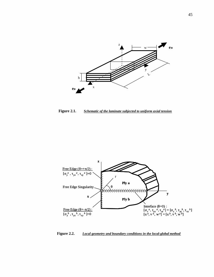
45
z
y
x
Lh
w
εo
εo
Figure 2.1. Schematic of the laminate subjected to uniform axial tension
Figure 2.2. Local geometry and boundary conditions in the local-global method
Ply α
Ply β
θ
r
y
z
Interface (θ=0) :[σz
α, τyzα, τxz
α] = [σzβ, τyz
β, τxzβ]
[u α, v α, w α] = [u β, v β, w β]Free Edge (θ=-π/2) :
Free Edge (θ=+π/2) :[σy
α , τyzα, τxy
α ]=0
[σyβ , τyz
β, τxyβ ]=0
Free Edge Singularity
x
Ply α
Ply β
θ
r
y
z
Interface (θ=0) :[σz
α, τyzα, τxz
α] = [σzβ, τyz
β, τxzβ]
[u α, v α, w α] = [u β, v β, w β]Free Edge (θ=-π/2) :
Free Edge (θ=+π/2) :[σy
α , τyzα, τxy
α ]=0
[σyβ , τyz
β, τxyβ ]=0
Free Edge Singularity
x
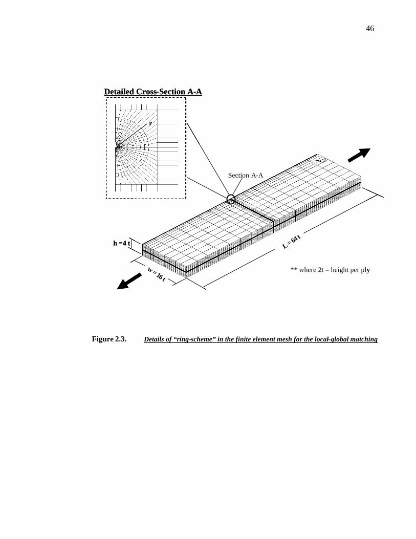
46
L = 64 t
w = 16 t
h =4 t
Section A-A
Detailed Cross-Section A-A
** where 2t = height per ply
r
L = 64 t
w = 16 t
h =4 t
Section A-A
Detailed Cross-Section A-A
** where 2t = height per ply
r
Figure 2.3. Details of “ring-scheme” in the finite element mesh for the local-global matching
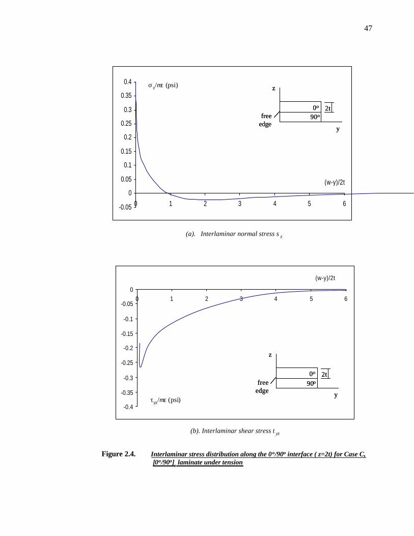
47
-0.4
-0.35
-0.3
-0.25
-0.2
-0.15
-0.1
-0.05
00 1 2 3 4 5 6
(w-y)/2t
Figure 2.4. Interlaminar stress distribution along the 0o/90o interface ( z=2t) for Case C,[0o/90o]s laminate under tension
(a). Interlaminar normal stress σz
(b). Interlaminar shear stress τyz
-0.05
0
0.05
0.1
0.15
0.2
0.25
0.3
0.35
0.4
0 1 2 3 4 5 6
(w-y)/2t
z
y
0o
90o2t
freeedge
z
y
0o
90o2t
freeedge
z
y
0o
90o2t
freeedge
z
y
0o
90o2t
freeedge
σz/µε (psi)
τyz/µε (psi)

48
Figure 2.5. Angular variation match between local and global stress solutions at various rings (r)for Case A [Matrix/Fiber], λ=-0.308.
(a). angular match for σzz
(b). angular match for τyz
Case A
-0.4
-0.35
-0.3
-0.25
-0.2
-0.15
-0.1
-0.05
0-100 -50 0 50 100
Singular
r=0.0002
r=0.002
theta
Case A
-0.07
-0.06
-0.05
-0.04
-0.03
-0.02
-0.01
0
0.01
0.02
-100 -50 0 50 100
Singular
r=0.0002
r=0.002
theta
σz

49
Figure 2.6. Angular variation match between local and global stress solutions at various rings (r)for Case B [0o/90o]s, λ=-0.0766.
(a). angular match for σz
(b). angular match for τyz
Case B
-0.01
-0.008
-0.006
-0.004
-0.002
0-100 -50 0 50 100
Singular
r=0.00004
r=0.0004
r=0.004
theta
Case B
-0.03
-0.028
-0.026
-0.024
-0.022
-0.02
-0.018
-0.016
-0.014
-0.012
-0.01-100 -50 0 50 100
theta
Singular
r=0.00004
r=0.0004
r=0.004σz

50
Figure 2.7. Angular variation match between local and global stress solutions at various rings (r)for Case C [0/90]s, λ=- 0.0344.
(a). angular match for σz
(b). angular match for τyz
Case C
-0.028
-0.023
-0.018
-0.013
-0.008
-0.003
0.002
-100 -50 0 50 100
Singular
r=0.00004
r=0.0004
r=0.004
r=0.04
theta
Case C
-0.009
-0.008
-0.007
-0.006
-0.005
-0.004
-0.003
-0.002
-0.001
0-100 -50 0 50 100
Singular
r=0.00004
r=0.0004
r=0.004
r=0.04
theta
σz

51
Figure 2.8. Log of the interlaminar normal stress (σz) plotted against the log of the radial distance (r). Slope of the plot is used to estimate the singularity strength (λ).
(a). Case B [0/90] s, λ=-0.0766
(b). Case C [0/90] s, λ=-0.0344
-0.8
-0.6
-0.4
-0.2
0
0.2
0.4
0.6
0.8
1
0 2 4 6 8 10 12 14 16 18
-log(r/2t)
FEA
Trend Line
Slope
y = -0.55151Ln(x) + 0.89132
(λ)
x
x
λ = -0.0344
r* = 1.3 x 10⁻¹⁷
-2
-1.5
-1
-0.5
0
0.5
1
1.5
2
2.5
0 2 4 6 8
-log(r/2t)
FEA
Trend Line
Slope
y = -0.61281Ln(x) + 1.74583
(λ)
x
x
λ = -0.0766
r* =1.0 x 10⁻⁸
log(σz/µε) psi
log(σz/µε) psi

52
CHAPTER 3: FREE EDGE STRESS GRADIENT ZONES
In the previous chapter, it is seen that singular points exist in the laminate
where distinct ply interfaces intersect the free edge. At each singularity, the stress state
becomes unbounded within a small vicinity of the singular point, and the strength of
the singularity is governed by the degree of mismatch in effective properties between
adjacent plies. At the same time, the laminate free edge stress field is also influenced
by a number of lamination parameters, such as ply fiber orientation, ply stacking
sequence, ply thickness, etc. Depending on how the lamination parameters are varied,
the structural interactions among the laminating plies can cause local stress
concentrations near the free edge that exist independently of the edge singularities. The
interlaminar stresses in the concentration zones can be comparable in magnitude to the
principle (in-plane) stresses.
In this chapter, the full field stress solutions are computed for a number of
select laminates. The effects of both the singular component and the lamination
parameter(s) component are included in the stress solutions. Emphasis is placed on the
magnitude and the size of the stress gradient zone (or “zone of dominance”) as
regulated by the computed components, individually and/or collectively. Analysis of
the stress gradient zones then provides a physical reasoning to the possible locations(s)
and the critical conditions for free edge delamination.

53
3.1. FREE EDGE STRESS GRADIENT ZONES IN [+θo/90on]s LAMINATES
Consider the [+θo/90on]s laminate series, where θ varies from from 0o, 15o, 25o,
35o, 45o, to 55o and n varies from 1/2, 1, 2, to 3. This particular stacking sequence is
chosen because not only singular points exist at particular ply interfaces, but also a
large tensile interlaminar normal stress, σz, concentration is produced in the stress field
when the laminate is loaded in axial tension. This σz concentration has been deemed as
a cause for delamination. Changes of each stress gradient zone are observed as the θ
and n parameters are varied, where the variation of θ controls the ply fiber orientation
of the outer two plies in the laminate, and the variation of n controls the thickness of
the middle 90o plies.
For specificity, assume the laminates have a finite width and its length is long.
The ply material properties for this laminates series are taken for a graphite-epoxy
system. The effective moduli are listed in Table 2.1, Case C. Each ply is of thickness,
2t.
3.1.1 Singular Points and their Strengths
There are two distinct edge singularities in each laminate in this series: one
located at the θo/-θo interface and the other at the -θo/90o interface. The singularity at
each interface is characterized by its strength, λ.
λ at the θo/-θo and the -θo/90o interface is calculated using the technique
described in Section 2.2.1. Figure 3.1 plots the λ values of both ply interfaces as
θ varies from 0o to 55o. At the θo/-θo interface, λ is seen to increase with the value of

54
θ; λ has a maximum of – 0.0275 when θ ∼ 50o. At this angle, the mismatch between
the θo/-θo ply properties is the largest. Beyond 50o, λ decreases to zero as θ approaches
90o; here, the both plies have the same ply properties and no singularity exists.
On the other hand, at the -θo/90o interface, λ is seen to decrease with the value
of θ; λ has the highest value of –0.035 when θ =0o; this is also the highest value of
λ for any θ in either interface. Again, λ converges to zero as θ approaches 90o.
A full field stress solution to include these singular stress fields is obtained
using the local-global stress matching method outlined in Section 2.2.2. With the value
of λ, the coefficients Ak in eigenvector X is determined within a scaling factor using
Eq. (2.22). In turn, X is used to compute the angular variations, σ?i j(θ), of the local
stress field using Eq. (2.19). σ?i j(θ) is then used to match the angular variations of the
global stress solution, rendered by the finite element solution.
Overall, λ at any θ angle is seen to relatively weak; the singularity strengths are
an order of magnitude smaller than crack-tip singularity (λ = −0.5). The stress
matching zone, consequently, is also small. Even for the highest value of λ= –0.035 at
the 0o/90o interface, the matching zone is estimated in the range of 10-15. 2t, which is
less than one fiber diameter from the free edge. This implies tha t the region in which
the singular solution dominates the laminate stress field is essentially zero, and the
laminate response is controlled mainly by the laminate parameters (ply orientation,
stacking sequence, etc.) and laminate loading. Here, the finite element solution seems
sufficient to provide the full field stress solution, including the singularity.

55
3.1.2 Stress Concentration Zones and Zone of Dominance Analysis
In this laminate series, the +θo plies are used to carry most of the in-plane
loading (particularly when θ is closer aligned with the 0o), while the 90o plies are
subjected to secondary stresses. Consider the +θo plies as one sub-unit in the laminate
and the 90no plies as another sub-unit. A mismatch in compliance can exist between
these two sub-units depending on the value of θ. Figure 3.2 plots the vxy of the +θ
grouped plies and the 90no plies, where vxy is the poison’s ratio of the respective sub-
units. While vxy of the 90no is constant at about 0.02, the vxy of the +θ plies can range
from 0.25 to 0.7. Note that vxy of the +θ plies is an order of magnitude higher than the
90o plies for any θ. The mismatch in vxy between the two sub-units is largest when θ is
in the 25o to 35o range.
Under tensile loading, the poisson mismatch produces a strong coupling
between the axial extension and bending when the plies are bonded together. Since the
+θ sub-unit is more compliant in the transverse direction, these plies tend to contract
more relative to the 90no plies. The result is a pulling effect normal to the 90n
o plies, and
is reflected by a large interlaminar normal stress concentration, σz, near the laminate
mid-plane.
To illustrate, Figure 3.3 (a) plots the interlaminar normal stress distribution, σz,
for the θ = +25o case, rendered by the ANSYS finite element software package. Here,
the σz distribution is shown along the 25o/-25o, -25o/90o, and 90o/90o interfaces. σz is
scaled by the applied axial strain, εo= 1 µε, and is plotted against the normalized
distance (y/2t) from the free edge.

56
As shown, σz is singular along the 25o/-25o and the -25o/90o interfaces. At the
former interface, σz is compressive near the laminate free edge, and has the sharpest
stress gradient among the interfaces due to its weak singularity, λ = -0.00638. At the
latter interface, σz is tensile near the free edge but is also unbounded; the tensile zone
extends to about one and half ply thickness into the laminate interior. λ at this interface
is -0.0305.
The 90o/90o interface (mid-plane), on the other hand, is also shown to have a
large tensile σz. σz does not rise as quickly compared to the singular interfaces and has
a finite value at the free edge. The maximum value for σz is about 2.7 psi/µε. When
compared to the axial stress (σx~ 2 psi/µε), the σz stress concentration at this interface
can be as significant as the singular interfaces.
Based the σz magnitudes alone, it is difficult to evaluate which effect, whether
the singular component or the stress concentration from the poisson mismatch
component, is more dominate in the σz stress field. It is therefore propose that, in
addition to magnitude, size of the gradient stress zone is also an important feature in
the laminate stress field.
Figure 3.3 (b) shows the σz/µε stress contour for a cross section of the
[+25o/90o]s laminate. Only one quarter of the laminate cross section is shown due to
symmetry. The y-axis represents the distance from the free edge, and the z-axis
represents the distance from the laminate mid-plane; both are normalized by the ply
thickness, 2t. For comparative purposes, the size of stress gradient zones is measured
by the number of fiber diameters existing within threshold level of the stress field.
Here, the threshold level of 1 psi/µε is chosen, which is approximately half of the

57
transverse strength of the 90o ply (normal to fiber direction). A fiber volume fraction of
60% is assumed, and there are approximately 15 fibers per ply thickness. The size of
stress zone within the threshold stress will be referred to as the “zone of dominance,”
or ZOD.
In the figure, the regions in the blue color denote tensile σz within the 1
psi/µε threshold level, while regions in black denote compressive σz. All other regions
are approximately zero and are not of significance. At the +25o/-25o interface, the
singular stress zone is in compression but is highly confined to the immediate region
near the free edge. Size of the singular stress zone is reduced to almost a single point in
the stress contour; and the ZOD is computed to be less than 1 fiber diameter. The small
size of the singular zone reflects the weak singularity strength at this interface.
For the mid-plane interface, however, the tensile σz stress concentration zone
appears to be much larger than the +25o/-25o interface. It is shown to be distributed in a
quarter circle pattern around the laminate mid-plane near the free edge (actually, the
full stress concentration zone is a half circle pattern since only a laminate quarter is
analyzed here). The stress zone extends to about half ply thickness into laminate width,
and covers the entire 90o ply thickness, ending slightly above at the -25o/90o interface.
The ZOD is computed to be approximately 160 fiber diameters in the laminate quarter
space. It is clearly the most dominate stress gradient zone in the σz field.
The size of the singular stress zone at the +25o/-90o interface is also small, and
appears to confined to the immediate region near the free edge. But, the ZOD could be
determined exactly because the stress concentration at the mid-plane extends into this
interface.

58
Actually, σz is not the only stress component that is singular or concentrated in
the [+25o/90o]s laminate. The interlaminar shearing stress, τyz, intensifies near the free
edge as well. Figure 3.4 (a) shows the τyz distribution along the three ply interfaces.
Although τyz is essentially zero at the mid-plane interface, τyz appears to be unbounded
approaching the free edge at the 25o/-25o and the -25o/90o interfaces. The stress
gradients at these interfaces are due to a combination of an edge singularity and edge
stress concentration. The edge singularity exists for reasons already discussed. The
stress concentration, on the other hand, is caused by extensional shear coupling
between the plies of different fiber orientations.
Figure 3.4 (b) plots the τyz/µε stress contour for a laminate cross section, with
the 1 psi/µε threshold stress imposed. Unlike σz, the most dominant stress zone is no
longer at the mid-plane, but lies at the +25o/-25o interface; the ZOD at this interface is
441 fibers. This is the largest stress gradient zone in either the τyz or σz fields. It is
unclear whether the effects of the edge singularity added to the stress concentration
size in this case.
The -25o/90o interface also exhibits a region of concentrated shear stresses near
the free edge, but of considerably smaller in size; this region covers approximately 6
fibers. All other regions in the τyz stress field are approximately zero.
In regards to delamination failure, the importance of the ZOD in the σz and τyz
stress fields will be discussed later in this chapter. But, for now, it is noted that the
computed ZOD are specific to [+25o/90o]s laminate case. These values will change if
the laminate configuration varies.

59
3.1.3 Poisson’s Ratio Mismatch Effect
As mentioned above, the tensile σz stress concentration zone at the [+25o/90on]s
mid-plane is the result of the mismatch in poisson ratio, vxy, between the +25o sub-unit
and the 90o sub-unit. Consider now the [+θο/90o]s laminate series, where the +θ
grouped plies is varied from 0o, 15 o, 25 o, 35 o, 45 o and 55 o. Here, θ varies the vxy of
the +θ grouped plies.
Figure 3.5 (a) – (f) plots the interlaminar normal stress, σz/µε, contour for each
laminate in this series subjected to axial strain, εo= 1 µε. Colors in red are tensile σz,
while colors in blue are in compression. Darker shades of each color denote higher
stress intensity. All other colors are approximately zero stress and are not of
significance.
For θ = 0o stress contour, σz stress concentration zone at the mid-plane is zero
(ZOD = 0); the maximum value of σz along this interface is also relatively small, σz =
0.44 psi/µε. The ZOD at all the other ply interfaces, including the singular stress zone
at the 0o/90o, is also zero. The σz stress concentration zones are non-existent in this
laminate because the mismatch of poisson ratio between the grouped +0o plies and the
90o ply is minimized; vxy of the +0o plies is 0.21.
However, as the θ value increases, the mismatch of poisson ratio between
grouped +θ plies and 90o ply increases; in turn, the σz concentration zone becomes
larger. The largest sized stress concentration zone occurs when θ = 35o, where the vxy
of the +35o plies is maximum at 0.677. The ZOD at the mid-plane is 194 fiber
diameters The overall stress intensity within the stress concentration zone is also
highest at this angle, as indicated by the dark shades of red in the stress contour ; the

60
maximum value of σz along the mid-plane is 3.1 psi/µε. Note that ZOD of the singular
stress zones at the θo/-θo and the -θo/90o interfaces does not change; they remains at
zero for all θ values.
For θ greater than 35o, the poisson mismatch effect is reduced, where the size
and overall stress intensity of σz concentration zone decreases in the mid-plane. Table
3.1 is a summary of these results; it correlates the poisson ratio of the +θ grouped plies
with the ZOD of the stress concentration zone and maximum σz value at the mid-plane.
It should be pointed out that the correlation among these parameters is not exact. For
example, the ZOD and max σz of the θ = 45o case are approximately the same as
θ = 25o, despite the latter angle having a smaller vxy. This suggests that there are other
factors, besides the poisson mismatch effect, that can contribute to the σz stress
concentration.
3.1.4 90o Ply Thickness Effect
Consider the [+25o/90on]s laminate series, with n= ½, 1, 2, 3, subjected to axial
strain, εo= 1 µε.. Here, the ply fiber orientation of the outer plies is constant at 25o such
that the poisson mismatch between these plies and 90o is near maximum, while n varies
in the 90o plies thickness. Thickness of the +25o plies are constant.
Figures 3.6 (a) – (c) plots the interlaminar normal stress, σz/µε, contour for
each laminate in this series (n =1 is shown in Figure 3.5 (c)). The figure shows the
overall σz profile is the same for all n with the largest stress gradient zone located at
the laminate mid-plane. The size of the stress concentration zone, however, is clearly
larger with higher values of n. Specifically, the ZOD increases from 86 fiber diameters

61
for n= ½ to 444 fiber diameters for n = 3. Here, the σz stress concentration remains
distributed fully through the entire 90no plies even as the value of n increases. Thus, the
90o ply thickness effect appears to augment size of the stress concentration zone from
the poisson mismatch effect.
However, unlike the [+θο/90o]s laminate series, the overall intensity of the stress
concentration zone decreases when the ZOD is larger. The n=1/2 case, for example, is
the most intense tensile σz stress concentration zone near the free edge zone, as
indicated by the darker shades of red. The maximum σz value is computed to be 3.3
psi/µε along the mid-plane. The n=3 case, conversely, has the lowest overall stress
intensity, where the stress concentration is more evenly distributed through the 903o
plies. The maximum σz here is computed to be 1.5 psi/µε. As n increases, the
constraining effects from the outer +25o plies are reduced and the interlaminar stress
concentration zone is more evenly distributed through the 90no plies; hence, the overall
magnitude of the stress concentration zone is lower. Table 3.2 gives a summary of
these results.
3.2. POSSIBLE DELAMINATION LOCATIONS AND FAILURE CONDITIONS
To determine the possible delamination locations and failure conditions, the
laminate stress fields, specifically the effects of the ZOD, are analyzed for the
[+25o/90on]s laminate series. Associated experiments have been performed by
Crossman and Wang [7] on this series. In the experiments, T300/934 [+25o/90on]s
laminate coupons, n= ½ to 8, were tested under tension, and the delamination process
for each laminate was observed. Their observations included the location of

62
delamination for each laminate, the associated onset strain, and other cracking modes
that may occur during loading. For this analysis, however, only the n= ½, 1, 2, and 3
laminate cases are followed where the full laminate stress fields have been computed in
the previous section, and the results are compared to the experiments.
The results of the experimental study are discussed in detail in Chapter 1.
Briefly, the observations show that the location for free edge delamination initiates at
the laminate mid-plane in the n= ½ and 1 laminates. For the n= 2 and 3 cases,
delamination was observed to occur either at the mid-plane or the –25o/90o interface.
Failure of the later interface was precipitated by the formation of transverse cracks.
Observations show that edge delamination is the first mode of failure when n < 2;
when n > 2, however, transverse cracking is observed to occur prior to any other failure
mode.
3.2.1. Delamination Location and Mode of Failure
For those laminates that delaminated without transverse cracks, the computed
σz stress field in the previous section shows that the -25o/90o and mid-plane interfaces
are possible delamination locations. Both have a large tensile σz near the free edge (σz
in the +25o/-25o interface is compressive, and therefore, unlikely to delaminate).
However, even though σz at the -25o/90o interface is singular at the free edge, the ZOD
at the mid-plane is orders of magnitude larger. The larger ZOD contains a greater
amount of strain energy due to its size and stress intensity within the zone. This strain
energy is believed to be the driving force for delamination to occur. Based on this

63
assumption, the mid-plane appears to be the more likely than the -25o/90o interface to
delaminate; this coincides with the experiment.
It should be noted that delamination in the above cases is essentially in an
opening mode (mode I) caused by the σz concentration. However, it is also possible
that delamination may be caused by failure modes other than σz. The stress analysis
shows that τyz is also concentrated near the free edge that can cause an out-of-plane
mode (or mode III) of failure. The other interlaminar shear, τxz, responsible for in-plane
mode (or mode II) is relatively small, and is negligible here.
Although laminates are generally stronger against the shearing stress than
normal stress, τyz may play a more significant role in delamination failure under
compression or fatigue loading. For instance, if the laminates are under compression,
the σz contour plot reverses sign such that the tensile stress zones become compressive,
and compressive stress zones become tensile. In such case, mid-plane delamination is
not expected because the σz is negative at this location.
The τyz stress concentration, on the other hand, remains the same despite the
sign change, where +25o/-25o interface is still the most dominant interface. Hence, in
compression loading (or possibly in fatigue loading), delamination is more likely at
occur at the +25o/-25o interface. Experimental data for this laminate under compressive
loading are not readily available, but a similar observation was noted in the T300-
S2/1034C [+30o/90o]s hybrid laminate under axial compression [54]. Here,
delamination at the +30o/-30o interface is observed as the first mode of failure.

64
3.2.2. Delamination Onset Strain
The onset of delamination in the [+25o/90on]s laminate series is caused mainly
by the tensile σz stress in the 90o ply near the free edge. In this sense, (σz)90 represents
the in-situ strength of the laminate for delamination. Table 3.3 compares the observed
onset load for delamination for this laminate series with the critical (σz)90 in the 90o
ply. The onset load is measured in terms of the tensile laminate strain, ε. The critical
(σz)90 is defined as the maximum σz/µε value along the mid-plane (listed on Table 3.2)
multiplied by the onset strain.
The table shows that the onset strain for delamination is approximately at 0.6%
for all the laminates in this series; i.e., the laminates fail at the same strain. The critical
(σz)90, however, varies with the value of n. Specifically, critical (σz)90 is seen to
decrease with the increase in the 90o ply thickness; the critical (σz)90 is at 20.2 ksi for
n=½ but drops to 8.6 ksi for n= 3.
The reason for the critical (σz)90 dependence on the 90o thickness may be found
by observing the ZOD with n (also listed in Table 3.3). The ZOD is computed to
approximately double with the increments of n; hence, the total amount of energy
available for delamination is increased. With this increase in energy, a lower critical
(σz)90 is needed for delamination to occur, even for the same applied strain.

65
3.2.3. Transverse Cracking vs. Delamination Transverse cracks are generally attributed to the in-plane tensile stress, σx,
which is also concentrated throughout the 90o plies. There can be an interaction effect
between the transverse cracks and delamination, where one may instigate the other.
Figure 3.7 plots the σz and σx values in the [+25ο/90no]s laminate series against
the value of n. Values of both stress components are taken at their maximums along
the mid-plane interface. Here, it is seen that σz is highest at 3.5 psi/µε when n =1/2 and
decreases with n. σz is about 1.3 psi/µε when n =3. σx, on the other hand, remains
relatively unchanged with n, about 2.5 psi/µε. The transition when σx becomes greater
than σz occurs between n = 1 to 2; this transition might explain why transverse
cracking is seen prior to delamination for the n > 2 laminates, while visa versa for the n
< 2 laminates.
While transverse cracks themselves are not generally catastrophic to the
laminate, they produce localized stress concentrations at their crack tips. When coupled
with the large σz concentration zone at the free edge, an interaction between transverse
cracking and edge delamination can occur. In such case, the onset of delamination can
be expedited, as indicated by the lower onset strain for delamination when the n > 2
laminates.
For completeness, Figure 3.8 plots the σz and σx values in the [+θο/90o]s
laminate series against the value of θ. Here, σz varies widely with θ, ranging from 0.5
to 3 psi/µε. Note that σz distribution follows the vxy distribution (see Figure 3.2),
reflecting the effects of the poisson mismatch. On the other hand, σx remains roughly

66
the same at 2 psi/µε. σz is the dominant stress component when θ is between 25-45o.
Hence, free edge delamination is likely the first mode of failure in this θ range.
Otherwise, σx governs the stress field? and transverse cracking may possible occur.
3.3. DISCUSSION
Edge delamination in laminates is shown to occur when interlaminar stress
gradient zones are present and are fully developed near the free surface. The zone of
dominance (ZOD) appears to play a more significant role than the stress magnitudes in
the delamination process. In this regard, free edge singularities, at least by themselves,
have been shown to have minimal influence on the overall stress field. Although the
stresses are infinite at the singular point, the strength of the singularity is relatively
weak and the associated size of the singular stress zone is small. Stress concentration
zones, on the other hand, can occupy regions in the laminate stress field orders of
magnitude larger than singular stress zones. Here, the ZOD from the stress
concentration zone is shown to be strongly influenced by the lamination parameters.
At this point, it should be noted that the ZOD can only identify the most likely
location for delamination failure, but cannot determine whether or not that particular
location(s) will delaminate under a given load. To predict the failure occurrence
requires a specific criterion. In the next chapter, the effective flaw concept, in
conjunction with a fracture mechanics approach, is described to predict the onset and
growth of delamination.

67
Table 3.2. Numerical results of the 90o ply thickness effect for the [+25o/-25o/90on]s laminate
series under axial tension
Table 3.1. Numerical results of the poisson's mismatch effect for the [+θo / -θo /90o]s laminate series under axial tension
~ 82 fibers1.77 psi/µε.370θ = 55o
~ 158 fibers2.71 psi/µε.550θ = 45o
~ 194 fibers3.09 psi/µε.677θ = 35o
~ 158 fibers2.73 psi/µε.662θ = 25o
~ 77 fibers1.58 psi/µε.496θ = 15o
~ 0 fibers0.44 psi/µε.210θ = 0o
Zone of Dominance(σz > 1 psi/µε)
Maximum σz along the mid-plane
vxy
[+θ]Laminate Series
~ 82 fibers1.77 psi/µε.370θ = 55o
~ 158 fibers2.71 psi/µε.550θ = 45o
~ 194 fibers3.09 psi/µε.677θ = 35o
~ 158 fibers2.73 psi/µε.662θ = 25o
~ 77 fibers1.58 psi/µε.496θ = 15o
~ 0 fibers0.44 psi/µε.210θ = 0o
Zone of Dominance(σz > 1 psi/µε)
Maximum σz along the mid-plane
vxy
[+θ]Laminate Series
~ 444 fibers1.45 psi/µεn = 3
~ 320 fibers1.89 psi/µεn = 2
~ 158 fibers2.73 psi/µεn = 1
~ 86 fibers3.31 psi/µεn = 1/2
Zone of Dominance(σz > 1 psi/µε)
Maximum σz along the mid-plane
Laminateseries
~ 444 fibers1.45 psi/µεn = 3
~ 320 fibers1.89 psi/µεn = 2
~ 158 fibers2.73 psi/µεn = 1
~ 86 fibers3.31 psi/µεn = 1/2
Zone of Dominance(σz > 1 psi/µε)
Maximum σz along the mid-plane
Laminateseries
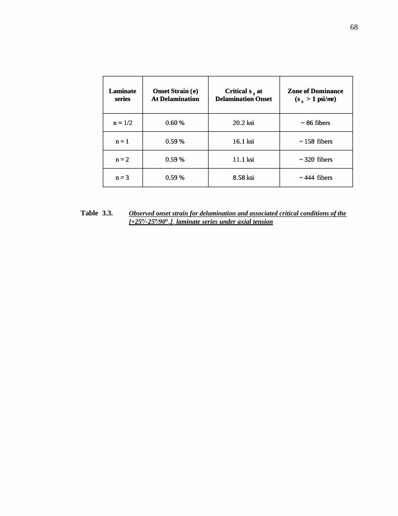
68
Table 3.3. Observed onset strain for delamination and associated critical conditions of the [+25o/-25o/90o
n]s laminate series under axial tension
8.58 ksi
11.1 ksi
16.1 ksi
20.2 ksi
Critical σz at Delamination Onset
0.59 %
0.59 %
0.59 %
0.60 %
Onset Strain (ε)At Delamination
~ 444 fibersn = 3
~ 320 fibersn = 2
~ 158 fibersn = 1
~ 86 fibersn = 1/2
Zone of Dominance(σz > 1 psi/µε)
Laminateseries
8.58 ksi
11.1 ksi
16.1 ksi
20.2 ksi
Critical σz at Delamination Onset
0.59 %
0.59 %
0.59 %
0.60 %
Onset Strain (ε)At Delamination
~ 444 fibersn = 3
~ 320 fibersn = 2
~ 158 fibersn = 1
~ 86 fibersn = 1/2
Zone of Dominance(σz > 1 psi/µε)
Laminateseries

69
Figure 3.2 Poisson ratio of the grouped [+θo/-θo] plies and the 90on plies in the [+θo/-θo/90o
n] slaminates series
Figure 3.1 Strength of edge singularity(s) at θo/-θo and the-θo/90on interface in the
[+θo/-θo/90on]s laminate series
0
0.1
0.2
0.3
0.4
0.5
0.6
0.7
0.8
0 10 20 30 40 50 600
0.1
0.2
0.3
0.4
0.5
0.6
0.7
0.8
0 10 20 30 40 50 60
θο
vxy
+ θo plies
90no plies
0
0.005
0.01
0.015
0.02
0.025
0.03
0.035
0.04
10 20 30 40 50 60
- λ
θο
θo /−θo interface
−θo /90o interface
0
0.005
0.01
0.015
0.02
0.025
0.03
0.035
0.04
10 20 30 40 50 60
- λ
θο
θo /−θo interface
−θo /90o interface

70
(b). σz/ µε stress contour plot with threshold stress, 1 psi/ µε, imposed
(a). σz/ µε stress distribution along the various interfaces
Figure 3.3 Interlaminar normal stress plots for [+25ο/ -25 o/90o]s laminate under tension
+25o
-25o
90o
y/2t distance from free edge
z /2
t di
stan
ce fr
om m
id-p
lane
σz/ µε
+25o
-25o
90o
y/2t distance from free edgey/2t distance from free edge
z /2
t di
stan
ce fr
om m
id-p
lane
z /2
t di
stan
ce fr
om m
id-p
lane
σz/ µε
-2
-1.5
-1
-0.5
0
0.5
1
1.5
2
2.5
3
0 1 2 3 4 5 6 7 8
(w-y)/2t (distance from free edge)
σz/ µε (psi)
+25/-25 interface
-25/90 interface
90/90 (mid-plane)
+25/-25 interface
-25/90 interface
90/90 (mid-plane)
(psi)
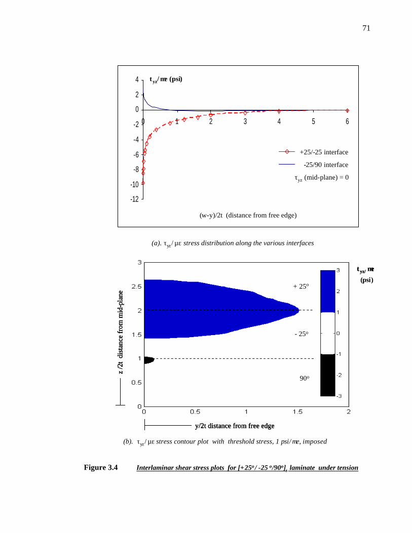
71
(b). τyz/ µε stress contour plot with threshold stress, 1 psi/ µε, imposed
(a). τyz/ µε stress distribution along the various interfaces
Figure 3.4 Interlaminar shear stress plots for [+25ο/ -25 o/90o]s laminate under tension
-12
-10
-8
-6
-4
-2
0
2
4
0 1 2 3 4 5 6
+ 25o
- 25o
90o
y/2t distance from free edge
z /2
t di
stan
ce fr
om m
id-p
lane
τyz/ µε
+ 25o
- 25o
90o
y/2t distance from free edgey/2t distance from free edge
z /2
t di
stan
ce fr
om m
id-p
lane
z /2
t di
stan
ce fr
om m
id-p
lane
τyz/ µε
(w-y)/2t (distance from free edge)
τyz/ µε (psi)
+25/-25 interface
-25/90 interface
τyz (mid-plane) = 0
(psi)

72
(b). θ =15o, σz/ µε stress contour plot near the laminate free edge
(a). θ =0o, σz/ µε stress contour plot near the laminate free edge
Figure 3.5 Interlaminar normal stress contours for [+θ/-θ/ 90]s laminate series under tension
σz/ µε
0o
0o
90o
z /2
t di
stan
ce fr
om m
id-p
lane
σz/ µε
0o
0o
90o
z /2
t di
stan
ce fr
om m
id-p
lane
z /2
t di
stan
ce fr
om m
id-p
lane
+15o
-15o
90o
y/2t distance from free edgey/2t distance from free edge
z /2
t di
stan
ce fr
om m
id-p
lane
z /2
t di
stan
ce fr
om m
id-p
lane
σz/ µε
y/2t distance from free edgey/2t distance from free edge
(psi)
(psi)
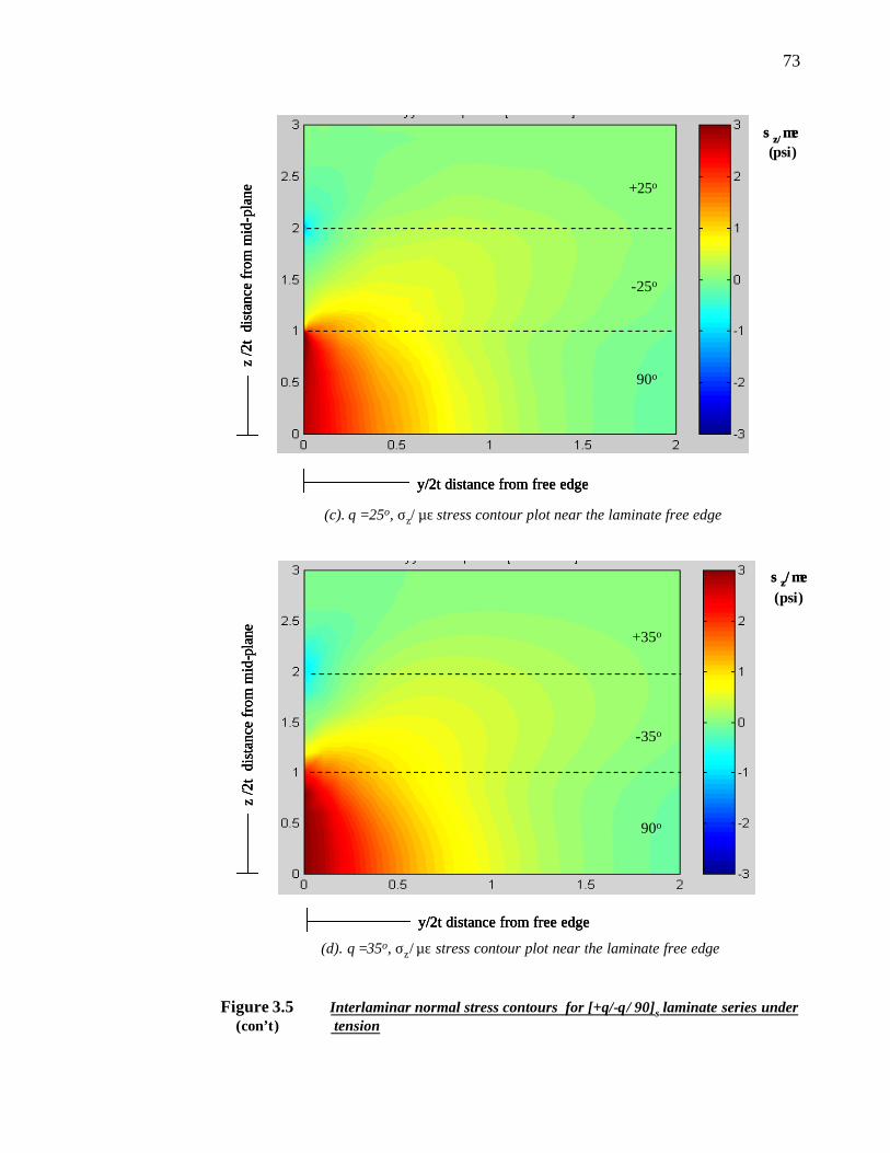
73
(d). θ =35o, σz/ µε stress contour plot near the laminate free edge
(c). θ =25o, σz/ µε stress contour plot near the laminate free edge
Figure 3.5 Interlaminar normal stress contours for [+θ/-θ/ 90]s laminate series under (con’t) tension
+35o
-35o
90o
y/2t distance from free edge
z /2
t di
stan
ce fr
om m
id-p
lane
σz/ µε
+35o
-35o
90o
y/2t distance from free edgey/2t distance from free edge
z /2
t di
stan
ce fr
om m
id-p
lane
z /2
t di
stan
ce fr
om m
id-p
lane
σz/ µε
+25o
-25o
90o
y/2t distance from free edge
z /2
t di
stan
ce fr
om m
id-p
lane
σz/ µε
+25o
-25o
90o
y/2t distance from free edgey/2t distance from free edge
z /2
t di
stan
ce fr
om m
id-p
lane
z /2
t di
stan
ce fr
om m
id-p
lane
σz/ µε
(psi)
(psi)

74
(d). θ =55o, σz/ µε stress contour plot near the laminate free edge
(c). θ =45o, σz/ µε stress contour plot near the laminate free edge
Figure 3.5. Interlaminar normal stress contours for [+θ/-θ/ 90]s laminate series under (con’t) tension
+45o
-45o
90o
y/2t distance from free edge
z /2
t di
stan
ce fr
om m
id-p
lane
σz/ µε
+45o
-45o
90o
y/2t distance from free edgey/2t distance from free edge
z /2
t di
stan
ce fr
om m
id-p
lane
z /2
t di
stan
ce fr
om m
id-p
lane
σz/ µε
+55o
-55o
90o
y/2t distance from free edge
z /2
t di
stan
ce fr
om m
id-p
lane
σz/ µε
+55o
-55o
90o
y/2t distance from free edgey/2t distance from free edge
z /2
t di
stan
ce fr
om m
id-p
lane
z /2
t di
stan
ce fr
om m
id-p
lane
σz/ µε
(psi)
(psi)

75
(b). n=2, σz/ µε stress contour plot near the laminate free edge
(a). n= 1/2, σz/ µε stress contour plot near the laminate free edge
Figure 3.6 Interlaminar normal stress contours for [+25/-25/ 90n]s laminate series under tension
+25o
-25o
90o
90o
y/2t distance from free edge
z /2
t di
stan
ce fr
om m
id-p
lane
σz/ µε
+25o
-25o
90o
90o
y/2t distance from free edgey/2t distance from free edge
z /2
t di
stan
ce fr
om m
id-p
lane
z /2
t di
stan
ce fr
om m
id-p
lane
σz/ µε
90o
- 25o
+25o
y/2t distance from free edge
z /2
t di
stan
ce fr
om m
id-p
lane
σz/ µε
90o
- 25o
+25o
y/2t distance from free edgey/2t distance from free edge
z /2
t di
stan
ce fr
om m
id-p
lane
z /2
t di
stan
ce fr
om m
id-p
lane
σz/ µε
(psi)
(psi)
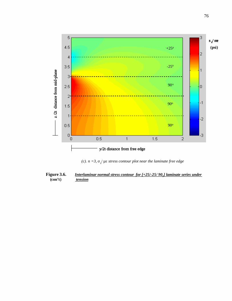
76
(c). n =3, σz/ µε stress contour plot near the laminate free edge
y/2t distance from free edge
+25o
-25o
90o
90o
z /2
t di
stan
ce fr
om m
id-p
lane
σz/ µε
90o
y/2t distance from free edgey/2t distance from free edge
+25o
-25o
90o
90o
z /2
t di
stan
ce fr
om m
id-p
lane
z /2
t di
stan
ce fr
om m
id-p
lane
σz/ µε
90o
Figure 3.6. Interlaminar normal stress contour for [+25/-25/ 90n] laminate series under (con’t) tension
(psi)

77
Figure 3.7. Maximum interlaminar normal and axial stress at the mid-plane as a function of the 90o ply thickness for [+25o/ -25o/ 90o
n]s laminate under tension
0
0.5
1
1.5
2
2.5
3
3.5
4
0 1 2 3 4
n
σ/µε (psi)
σx (axial)
σz (Int. norm)
σ/ue (psi)
0
0.5
1
1.5
2
2.5
3
3.5
-5 5 15 25 35 45 55
σ/µε (psi)
θ
σx (axial)
σz (Int. norm)
0
0.5
1
1.5
2
2.5
3
3.5
-5 5 15 25 35 45 55
σ/µε (psi)
θ
σx (axial)
σz (Int. norm)
Figure 3.8. Maximum interlaminar normal and axial stress plot at the mid-plane as a function of θ for [+θ/ -θ/ 90]s laminate under tension

78
CHAPTER 4: FREE EDGE DELAMINATION ANALYSIS
The purpose of this chapter is to outline the so-called “effective flaw” concept
for the free edge delamination initiation and growth analysis. The concept postulates
that random material flaws of microscopic size exist at the ply interfaces in laminates.
When the interlaminar stress field near the laminate free edge reaches a certain critical
level, one or more of the interlaminar micro-flaws may propagate into the a
delamination crack of macroscopic size. To render a predictive model, the integrated
effects of these micro-flaws are represented by an effective flaw located at the ply
interface most likely to delaminate. The effective flaw is treated as a physical edge
crack in the laminate, where fracture mechanics theory is then applied to predict the
critical load at the onset of delamination.
To illustrate this method of delamination analysis, the [+θο/90on]s laminate
series, with θ = 15o,25o,35o,45o and n =1/2, 1, 2, is used as examples. This series is
chosen because the full stress fields for these laminates have been computed in the
previous chapter, where the analysis of the “zone of dominance” serves to guide in the
placement of the effective flaw. Some experimental results are also available for this
laminate series.

79
4.1. THE EFFECTIVE FLAW CONCEPT
4.1.1 Effective Interlaminar Flaws
In the effective flaw concept, it is postulated that micro-flaws are present
throughout the laminate body. The flaws are either inherent to the laminate or
introduced during fabrication [43]. For delamination, consider only those micro-flaws
that exist along the ply interfaces near the laminate free edge; these flaws are called
interlaminar flaws since they are parallel to the ply interface and normal to the laminate
thickness direction. Figure 4.1 (a) shows a schematic of one ply interface of the
laminate, viewed at the micro-scale. The micro-flaws are shown to be randomly
distributed in the ply interface, where the sizes and shapes of each micro-flaw vary.
While the exact distribution of the micro-flaws is unknown, an effective flaw is
introduced to represent the collective effects of the micro-flaws. Figure 4.1 (b) shows a
schematic of the same ply interface as Figure 4.1 (a), viewed at the macro-scale. Here,
the interlaminar micro-flaws are replaced by one single interlaminar effective flaw
running uniformly along the free edge. The effective flaw size is denoted as ao, where
ao is a random quantity that has to be correlated by experiments. Under a critical
applied laminate loading, the effective flaw is assumed to grow and turn into the
physical delamination crack; this defines the onset of delamination. Upon onset,
delamination is treated as a uniform plane crack that propagates self-similarly into the
laminate interior (see Figure 4.1 (c)).
It is noted that interlaminar flaws can be present at each ply interface of the
laminate; however, depending on the type of laminate loading and the laminate

80
configuration, only a certain interface will delaminate (as discussed in Chapter 3). The
driving force for the flaw growth comes from the total amount of strain energy
available surrounding the flaw. For delamination, this energy is provided by the
interlaminar stress gradient zones that are present near the laminate edges. Hence, the
interface with a large or dominant interlaminar stress gradients zone is likely to
delaminate.
For a given laminate, then, the interlaminar stress field can be computed to
determine which interface will most likely delaminate; only effective flaws at these
locations need to be considered in the laminate model. To determine the critical load at
which the effective flaw becomes a delamination crack, a specific criterion is needed.
4.1.2 Fracture Criterion
The effective flaw is a hypothetical quantity; but it is treated as physical crack
in the analysis model. In such case, the linear elastic fracture mechanic theory can then
be applied. The theory proposes a force, G, that drives the crack comes from the elastic
strain energy stored in the crack-tip concentration zone. This force is resisted by the
material’s fracture toughness, Gc. The former is commonly known as the energy
release rate, and in general is a function of the applied load, e, and the crack size a. The
latter is commonly known as the critical energy release rate, and also is a function of a.
Then, for a crack size ao, the crack is said to propagate when the crack driving force is
equal to or greater than the material fracture toughness [55]:
G (a, e) = Gc at a=ao (4.1)

81
Crack growth may be stable or unstable depending how the rate of G varies
with the crack size a. If dG/da > dGc/da, then crack propagation is said to be unstable
because the rate of change in the crack driving force exceeds the rate of change of the
material’s resistance to crack growth. On the other hand, propagation is considered
stable when dG/da = dGc/da (if dG/da < dGc/da , then there is no crack growth).
In applying the above criterion to delamination, the location of the effective
flaw is first determined; namely, at the ply interface suspected to delaminate. Growth
of the flaw is then evaluated using Eq. (4.1), given the values of Gc and ao at this
interface. ao, as mentioned earlier, is a random variable that requires some statistical
measures in its determination; this is discussed in the next section. Gc, on the other
hand, is a material property that can be measured by experiment [56]. For the problem
considered, the Gc is measured mainly for an opening mode (mode I) failure, GIc. It has
been shown GIc is a constant value (i.e., independent of a) if a is significantly large.
In addition to Gc and ao, G of the propagating effective flaw also needs to be
calculated. A numerical technique for the computation of G has been described by
Wang [3]. It is an finite element approach based on so-called “crack-closure” scheme
[57], such that G is expressed explicitly in terms of the applied loading, e, and the
crack size a. Details of this approach are given in Appendix D. Let ex denote an applied
laminate strain in the axial direction. If thermal effects from laminate curing are
significant, then thermal residual effects also need to be included in G. Let ∆T = T –
To, where T is the temperature at laminate loading, and To is the temperature at the
laminate stress-free state (some regard this as curing temperature). From Wang [3], G
is then given as:

82
G (ex, ∆T, a) = [ Ce ex - CT ∆T ]2 2t*
(4.2)
or, in expanded form
G (ex, ∆T, a) = [ Ce ex
2 + CeT ex ∆T + CT ∆T2 ] 2t* (4.3)
where 2t* is a dimensionless scaling factor between the laminate model and the
physical laminate, and the coefficients Ce, CT, and CeT are the material “shape
functions,” associated the mechanical, thermal, and mixed loadings, respectively. They
are dependent on the crack size a and the ply elastic constants, but not on the applied
loading. Therefore, the general behavior of Ce, CT, and CeT is the same as the energy
release rate, G.
With the values of Ce, CT, and CeT for a given crack size a and an applied
laminate loading (ex and ∆T), G can be then computed by Eq (4.2) or (4.3). Figure 4.1
shows a schematic of the typical behavior of the energy release rate function G as a
function of a for delamination. It is seen that G rises sharply from a=0 and reaches a
maximum value Cmax at the knee of the curve, a=am; G remains relatively flat
afterwards, where crack growth appears to be stable. The asymptotic behavior of G
suggests that delamination growth is essentially a neutral, or at least, stable process. If
no other failure modes appear during the loading, the delamination crack then should
then grow uniformly towards the center of the laminate.
The exact meaning of am is not clearly understood but it seems to represent the
minimum size for which delamination is fully developed. In general, am is generally in

83
the range of two ply thicknesses, but its exact value depends on the local stress field
near the crack; hence, am varies with the laminate parameters.
4.1.3 The Range of the Effective Flaw Size
The last variable needed in the fracture criterion is determining the effective
flaw size, ao. From Eq. (4.3), it is seen that the applied load, ex, has a one to one
relationship with the crack size, a. Figure 4.3 shows a schematic of this relationship for
the condition G = GC. It is seen that ex decreases sharply from a=0 and reaches a
minimum value at a= am; ex remains relatively the same afterwards. Note that am is the
same crack size when G reaches its steady value.
Now, let the effective flaw size, ao, be a random variable; its distribution is
represented by some probability function f(ao) [3]. If all possible values of ao are
included in the f(ao), then there is a corresponding range of ex for which Eq. (4.3) is
satisfied. While exact f(ao) is not known, it is seen from the figure that ex has reached
its minimum value for a flaw size equal to am or greater; here, the minimum value of ex
represents the lower-bound onset strain.
While am is in the order of a ply thickness, the observable delamination crack is
order of a laminate thickness. It is probable that a flaw of size am or larger can be found
at some location along the laminate free edge, assuming the laminate is long in length.
Therefore, delamination onset can be predicted by the lower-bound value of ex
associated with ao > a. The predicted minimum critical strain for delamination onset is
then calculated from Eq. (4.2) with the condition in Eq. (4.1). This is given by:

84
at a > am (4.4)
where Ce and CT are its maximum value. In this context, determining the exact value of
ao or f(ao) becomes unnecessary.
4.2. DELAMINATION INITIATION
The delamination analysis described above is used to determine the onset of
free edge delamination for the [+θο/90on]s series. Consider first the [+25o/90o]s laminate
(i.e., θ=25o and n= 1). The material properties are taken for a graphite-epoxy laminate
system, and the ply material properties are given in Table 2.1, Case C; thickness of an
individual ply (2t) is 0.0052 inches. Thermal loading from the curing process is also
included, where temperature difference between the laminate stress free temperature
(To = 350oF) and temperature at loading (T= 75oF) is ∆T=-275oF. Thermal expansion
coefficients for the laminate are: αL = 2 x 10⁻⁷/oF, αT = αz = 1.6 x 10⁻⁵/oF.
The full interlaminar laminate stress field for this laminate has been computed
in the previous chapter. It was shown that 90o/90o (mid-plane) interface possesses a
dominant tensile σz stress concentration near the free edge. The zone of dominance
(ZOD) at this interface is computed to be 158 fiber diameters. This stress zone has
been thus blamed the mid-plane delamination found in the experiment.
Figure 4.4 shows the mechanical energy release coefficient Ce curve along the
mid-plane associated with the applied strain, ex. In this figure, Ce is plotted as a
function of the effective flaw size, a, propagating into the laminate interior. It is seen
ecr (Gc /2t*) + CT ∆T
Ce
=

85
that Ce sharply rises from a=0 (when no crack is present), and reaches a maximum
value Cemax = 4.0 x10⁶ lb/in2 when am= 2.2t. Ce remains constant afterwards.
For significantly large a, Ce is observed to decrease and eventually drop to zero
when a= 10.2t (not shown on the figure). This is due to the flaw growth approaching
the center of the laminate coupon, and the 90o/90o plies are nearly separated. In this
regard, stability of the crack growth depends on the width of the laminate, such that
wider coupons generally allow for a longer stable crack growth.
Figure 4.4 also shows the thermal energy release coefficient CT curve along the
mid-plane associated with the thermal load ∆T. The CT curve shares a similar shape as
Ce. CTmax is computed to be approximately 2.0 x10⁻⁴ lb/in2/F2 also at am= 2.2t. Note,
however, that CTmax is several orders of magnitude smaller than Cemax.
With the computed values of Ce and CT, the critical load for which the effective
flaw will grow into a delamination is determined by Eq. (4.4). For this laminate, the
critical energy release rate, Gc is measured at 1.3 lb/in [22]. Figure 4.5 shows the
relationship between the applied laminate strain, ex, and the crack size, a, satisfying the
condition in Eq (4.1). ex is shown to reach a minimum value at ecr = 0.59% when a >
2.2t; this is the lower-bound value used to predict the minimum delamination onset
strain. The corresponding σcr is 58.5 ksi (by using Hooke’s Law σcr = Ex ecr. with Ex =
9.6 Msi).
For comparison, tensile tests have been performed on T300/934 graphite epoxy
[+25o/90o]s laminate coupons [7]. It was observed that the first detection of
delamination growth is within the range of 0.58 to 0.61% strain. The predicted lower

86
bound strain falls within the range of the experimental values, and the size of the
effective flaw in this case is in the order of two ply thicknesses.
Similar comparisons for the other laminates in the [+θο/90on]s series are
reported in [7,22,44,57,58] using this delamination analysis. There, a good agreement
has been demonstrated between predicted onset values of delamination and the
experiments. Generally, the predicted lower-bound onset strain falls in the range of the
observed onset strain
.
4.2.1 Thermal Effects
The importance of the thermal loading effect is emphasized in the delamination
onset prediction of the [+25o/90o]s laminate. While the thermal shape function, CT, is
orders of magnitude smaller than the mechanical shape function, Ce, there is also the
mixed- loading component, CeT, that contributes to the energy release rate. CeT is a
represents the thermal-mechanical coup ling in the energy release rate. This component
was not directly calculated in the above example, but is included in the energy release
rate and the critical load prediction (see Eq.(4.2) vs. Eq (4.3)).
To see the individual contributions of Ce, CT, and CeT in the energy release
rate, consider the [+25o/90o]s laminate again, except that the thermal loading ∆T is
varied. Assume that the curing temperature remains the same (To = 350oF) but the
loading temperature ranges from a warm environment condition (T = 120oF) to a cold
environment condition (T =-20oF); i.e., ∆T varies from –230oF to – 370oF. The applied
laminate strain is ex =0.6%, which is about the observed onset strain for delamination
for this laminate.
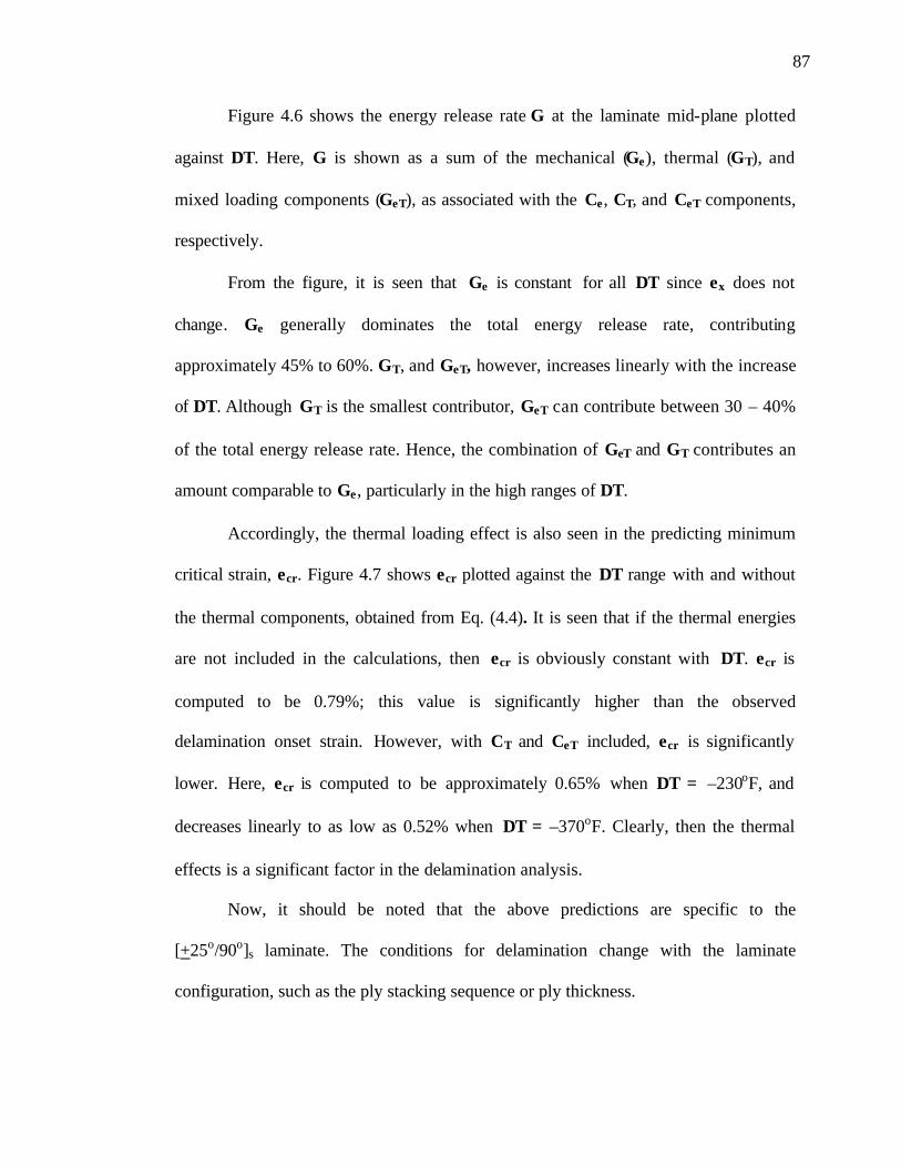
87
Figure 4.6 shows the energy release rate G at the laminate mid-plane plotted
against ∆T. Here, G is shown as a sum of the mechanical (Ge), thermal (GT), and
mixed loading components (GeT), as associated with the Ce, CT, and CeT components,
respectively.
From the figure, it is seen that Ge is constant for all ∆T since ex does not
change. Ge generally dominates the total energy release rate, contributing
approximately 45% to 60%. GT, and GeT, however, increases linearly with the increase
of ∆T. Although GT is the smallest contributor, GeT can contribute between 30 – 40%
of the total energy release rate. Hence, the combination of GeT and GT contributes an
amount comparable to Ge, particularly in the high ranges of ∆T.
Accordingly, the thermal loading effect is also seen in the predicting minimum
critical strain, ecr. Figure 4.7 shows ecr plotted against the ∆T range with and without
the thermal components, obtained from Eq. (4.4). It is seen that if the thermal energies
are not included in the calculations, then ecr is obviously constant with ∆T. ecr is
computed to be 0.79%; this value is significantly higher than the observed
delamination onset strain. However, with CT and CeT included, ecr is significantly
lower. Here, ecr is computed to be approximately 0.65% when ∆T = –230oF, and
decreases linearly to as low as 0.52% when ∆T = –370oF. Clearly, then the thermal
effects is a significant factor in the delamination analysis.
Now, it should be noted that the above predictions are specific to the
[+25o/90o]s laminate. The conditions for delamination change with the laminate
configuration, such as the ply stacking sequence or ply thickness.

88
4.2.2 Poisson’s Ratio Mismatch Effects
In the [+25o/90o]s laminate example, the driving force for delamination is
provided by the σz stress concentration zone at the laminate mid-plane. The σz stress
concentration at this laminate is mainly due to the mismatch in poisson ratio, vxy,
between the grouped +25o plies and the 90o plies. Consider now [+θο/90o]s laminate
series, with θ = 15o, 25o, 35o, and 45o, under axial tension. While the vxy of the 90o ply
remains constant at 0.02, the vxy of the grouped +θ plies varies from 0.25 to 0.7 It has
been shown that a larger mismatch of vxy between these ply groups produces a larger σz
zone of dominance (ZOD) at the laminate mid-plane. A comparison of the vxy of the
grouped +θ plies and the ZOD at the mid-plane is given in Table 3.1.
To observe how G varies with the poisson mismatch effects, Figure 4.8 shows
the Ce curves for mid-plane delamination in this laminate series. For simplicity, the
thermal loading is assumed zero. It is seen that Ce curves for all the laminates have
similar shapes, however Cemax is clearly larger for those laminates that have a higher
vxy of the +θ group plies. The θ=35o laminate has the highest Cemax computed to be 4.7
x 106 lb/in2 with the associated ZOD = 194 fiber diameters. This laminate therefore is
the most energetically favorable to delaminate among this series. Cemax value decreases
when θ changes in either direction, with θ=15o the least energetically favorable to
delaminate.
Correspondingly, the Ce curve takes longer to develop for the laminates with
the higher Cemax values. am for the θ=35o laminate is approximately 2.5.2t compared to
1.5.2t for the θ=15o laminate. Both the θ=25o and the θ=45o laminate appear fully
develop at about the crack size, am = 2.2t, since the ZOD are the same.

89
For comparative purposes, the delamination onset strain for this laminate series
is predicted, based solely on the mechanical energy component. In this series, the
θ=35o laminate has the lowest minimum critical strain at 0.73% and the θ=15o having
the highest minimum critical strain at 1.25%. This trend seems to show that the
predicted values are influenced strongly by the poisson mismatch effect, where
laminates that have a more prominent poisson effect tend to delaminate at a lower
applied load. However, experimental data could not be found for this particular
laminate series. For accurate predictions of the delamination onset, the thermal load has
to be included.
4.2.3 Ply Thickness Effects
Consider now the [+25ο/90no]s laminate series, with n=1/2, 1, and 2 , under axial
tension. Here, θ of outer plies is constant at 25o so that the poisson mismatch effect is
near maximum. n, on the other hand, varies the thickness of the 90o plies. It has been
shown that σz concentration zone remains fully distributed through the entire 90no plies
when the laminate is loaded; thus, the thicker 90o ply laminates in this series (i.e.,
higher values of n) have a larger sized σz concentration zone. A comparison between n
and the σz ZOD at the mid-plane is given in Table 3.2.
Figure 4.9 shows the Ce curves for this laminate series assuming mid-plane
delamination. The Ce curves for all the laminates have similar shapes, except that am
and Cemax seem to vary with n. For n=1/2, am is shown to be less than 1.2t; this is
because the ZOD for this laminate is the smallest among this series but has the highest

90
overall intensity with the stress concentration zone. Cemax for this laminate is computed
at 4.1 x 10⁶ lb/in2.
For n= 1 and 2, Ce are fully developed at about the crack size am = 2.2t and
2.5.2t, respectively. However, unlike the poisson mismatch effect, it appears that Cemax
becomes smaller with the increase of the ZOD; specifically, Cemax for n=1 is equal to
4.1 x 10⁶ lb/in2 compared to 3.5 x 10⁶ lb/in2 for n=2. Consequently, if the onset of
delamination is predicted based solely on the mechanical energy component for these
two laminates, the former is more energetically favorable for delamination with a
predicted onset strain of 0.79%; the predicted onset strain of the latter is 0.85%. A
summary of these results are given in Table 4.2.
The above statement is true if assuming that edge delamination is the only
failure event during the entire course of loading. In fact, experiments on this laminate
series have shown that, for the n = ½ and 1, edge delamination is the first damage
mode [7]. Predictions for the delamination onset strain appear to match well with the
observed onset strain when the thermal load is included. However, for the n=2
laminate, it has been observed that transverse cracking occurs prior to free edge
delamination. The presence of transverse cracks causes a locally complex state of stress
at the crack-tip that can interact with the delamination process; hence, the delamination
onset can be much lower than the predicted value based on this Ce curve.
Thus, the Ce curve computed here determines which laminates are likely to fail
by delamination; but, it does not necessarily predict whether delamination is the first
mode of failure. The effects of the transverse crack can lower the onset strain
prediction. A separate analysis can be performed to predict the onset of transverse
91
cracking using the same failure method used in this analysis. The effects transverse
cracking versus free edge delamination for this laminate series is documented in [22].
4.3. DELAMINATION GROWTH
The transition from free edge delamination initiation to delamination growth
occurs when the interlaminar effective flaw, ao, grows and becomes the delamination
crack. The transition in this delamination analysis is evaluated at the effective flaw
size, ao, which generally is an unknown variable. However, it appears that the initial
driving force for ao to grow comes from the local stress field near the free edge;
namely, the free edge interlaminar stress gradient zone. Once delamination occurs, ao is
no longer a hypothetical quantity flaw and the delamination crack itself causes local
stress concentration at the crack tip. This local stress concentration then drives the
crack to grow further into the laminate.
To further understand the mechanisms that drive the delamination initiation-
growth transition, consider the [+25o/90o]s example examined earlier in this chapter.
The effective flaw for this laminate is located at the mid-plane where delamination is
mostly to occur. Figure 3.3 (b) shows the σz contour plot for a laminate cross section
(computed in the previous chapter) when no crack is present. The σz concentration
zone, in this case, is caused by the mismatch in poisson ratio between the grouped +25o
plies and the 90o ply. This large tensile σz stress concentration zone is believed to be
the initial driving force for flaw to propagate.
As the flaw grows in the laminate, the σz field changes near the flaw, and a
transition is seen in the crack driving force from the free edge stress concentration to

92
local stress concentration at the crack-tip. Figure 4.10 (a-d) shows the σz stress contour
plots for an incremental flaw size, a/2t = 0.2, 0.4, 0.6, 0.8, along the mid-plane. A
threshold stress of σz> 1psi/ue is prescribed on the stress contour so that the ZOD can
be measured. The regions in the blue color in the contour represent the tensile σz above
the threshold stress.
At a/2t= 0.2, the size and shape of the σz stress concentration zone are
approximately same compared to when no crack is present. The stress zone is shown to
extend to about 0.7.2t into the laminate interior, and covers the entire 90o ply thickness
near the free edge. The ZOD is computed about 145 fiber diameters. Here, the effective
flaw is small, and its influence on the interlaminar stress field is minimal; the σz stress
field remains to be dominated by the poisson effects.
At a/2t= 0.4, the σz stress concentration zone is shown to shift away from the
laminate free edge and center around the crack tip itself. The stress zone extends from
the free edge to about 0.8.2t into the laminate interior. The ZOD decreases to about 135
fiber diameters. In this case, the flaw is sufficient in length to release some of
constraints of +25o plies on the 90o ply; hence, the decrease of the ZOD.
At a/2t= 0.6, the σz stress concentration separates into two zones: one centered
around the crack tip and the other near the free edge at the -25o/90o interface. Now, it
appears that the driving force for flaw growth is driven solely by the σz stresses around
the crack-tip. The ZOD of this stress zone is about 85 fibers diameters. The free edge
effect, however, remains at the -25o/90o interface as indicated by the small stress
concentration zone. This stress zone is considerably smaller (ZOD = 25 fibers
diameters) than the crack tip stress zone. At a/2t= 0.8, the shape and size of crack tip

93
stress concentration zone near the crack tip appear approximately the same as the
previous crack size.
While the ZOD becomes stable at 1 ply thickness, the intensity within the stress
σz magnitude continues to develop. Figure 4.11 compares the ZOD and the σz
magnitude at the crack tip as a function a flaw size a. Because σz is singular at the
crack tip, the σz value is averaged over a small region around from the singular point.
In this analysis, σz is averaged over a 15 fiber diameter region. It is seen that the ZOD
decreases quickly with a, and reaches a minimum value of 85 fibers diameters at about
one ply thickness. However, σzavg increases with a; it reaches a limiting value when the
crack size is about two ply thickness; σzavg maximum is computed at 2.8 psi/uε. This
shows that while the ZOD becomes smaller with a, the stress concentration zone is
more localized around the flaw.
Hence, ZOD and σzavg are both constant values when the flaw size is 2 ply
thicknesses. This is the same flaw size for which the energy release rate curve reaches a
constant value (i.e. a = am). It is here where delamination is said to be fully developed.
This seems plausible since the stress concentration zone reflects the amount of energy
available for the flaw to grow. As the stress concentration zone becomes stable, so does
the energy release rate.
4.4. DISCUSSION
The effective flaw is a necessary parameter in formulating the delamination
prediction model in this analysis. The flaw appears to retain the effects of the micro-
flaws leading up to delamination initiation that otherwise cannot be modeled at the

94
macro-scale. This idealization allows the delamination behavior to be described by a
fracture mechanics approach when used in conjunction with a three dimensional stress
analysis.
It is seen that growth of the flaw depends strongly on the local stress field near
the flaw tip. A flaw that exists within large or dominant interlaminar stress gradient
zone tends to release more strain energy during crack growth; hence, this type of flaw
is energetically favorable to grow and propagate. In this sense, the effective flaw
concept is able to include the zone of dominance of the free edge stress field, discussed
previously as an important feature in the delamination process.
While the effective flaw is an essential feature in the delamination model, the
exact size of the flaw could not be determined. The model can only predict the
minimum critical load for onset, based when the energy release rate of the flaw is
stable and delamination is already fully developed; the flaw size is generally on the
order of one to two ply thicknesses for the graphite-epoxy laminate examined.
However, in order to correlate a size of the effective flaw with this delamination model,
it is believed that the role of the micro-flaws needs to be understood. In such case, a
microscopic analysis of the laminate stress field may be necessary.

95
Table 4.1. Computed values of Cemax and am for the [+θo / -θo /90o]s laminate series, assuming mid-plane delamination.
Table 4.2. Computed values of Cemax and am for the [+25o?/ -25o?/ 90on]s laminate series,
assuming mid-plane delamination.
~ 2
~ 2.5
~ 2
~ 1.5
am
(per 2t)
3.3 x 10⁶~ 158 fibers.550θ = 45o
4.7 x 10⁶~ 194 fibers.677θ = 35o
4.0 x 10⁶~ 158 fibers.662θ = 25o
1.6 x 10⁶~ 77 fibers.496θ = 15o
Ce max
(lb/in2)Zone of Dominance
(σz>1 psi/µε)vxy
[+θ]Laminate
series
~ 2
~ 2.5
~ 2
~ 1.5
am
(per 2t)
3.3 x 10⁶~ 158 fibers.550θ = 45o
4.7 x 10⁶~ 194 fibers.677θ = 35o
4.0 x 10⁶~ 158 fibers.662θ = 25o
1.6 x 10⁶~ 77 fibers.496θ = 15o
Ce max
(lb/in2)Zone of Dominance
(σz>1 psi/µε)vxy
[+θ]Laminate
series
~ 2.5
~ 2
~ 1
am
(per 2t)
3.5 x 10⁶~ 320 fibersn = 2
4.0 x 10⁶~ 158 fibersn = 1
3.5 x 10⁶~ 86 fibersn = 1/2
Ce max
(lb/in2)Zone of Dominance
(σz>1 psi/µε)Laminate
series
~ 2.5
~ 2
~ 1
am
(per 2t)
3.5 x 10⁶~ 320 fibersn = 2
4.0 x 10⁶~ 158 fibersn = 1
3.5 x 10⁶~ 86 fibersn = 1/2
Ce max
(lb/in2)Zone of Dominance
(σz>1 psi/µε)Laminate
series

96
Figu
re 4
.1.
Eff
ectiv
e F
law
Con
cept
(a)
Mic
rosc
opic
vie
w
of a
ply
inte
rfac
e in
the
lam
inat
e:
Ran
dom
ly d
istri
bute
d m
icro
-fla
ws
(b)
Mac
rosc
opic
vie
w
of a
ply
inte
rfac
e in
the
lam
inat
e:E
ffec
tive
inte
rlam
inar
fla
w
of s
ize
“ a o
“on
the
free
edg
e
a oa o
(c)
Lam
inat
e un
der
axia
l loa
d:E
dge
dela
min
atio
n of
siz
e “ a
o“
on th
e fr
ee e
dge
x
yz
e x
e x
edge
de
lam
inat
ion
a o
x
yz
e x
e x
edge
de
lam
inat
ion
a o

97
Figure 4.2. Schematic of the energy release rate as a function of the crack size for free edge delamination.
Figure 4.3. Schematic of the range of the effective flaw size and the corresponding rangeof the onset strain for free edge delamination.
a
ex
G(a,ex)=Gc
am
Effective flaw size distribution f(ao)
OnsetLoadrange
a
G (a, ex)
am
Gmax
a
G (a, ex)
am
Gmax

98
Figure 4.4. Energy release rate shape functions for mid-plane delamination in the [+25o/ -25o
/90o]s laminate under tension.
Figure 4.5. Predicted onset strain (with G = Gcr) as a function of crack size for mid-plane delamination in the [+25o/ -25o /90o]s laminate under tension
0
0.5
1
1.5
2
2.5
3
3.5
4
4.5
0 0.5 1 1.5 2 2.5 3
a/2t
CT x 104 (F2/in2/lb)
Ce x 10-6 (in2/lb)
0.2
0.3
0.4
0.5
0.6
0.7
0.8
0.9
1
1.1
1.2
0 0.5 1 1.5 2 2.5 3
ex (%)
G(a,ex)=Gc
a/2t

99
Figure 4.7. Minimum critical strain as a function of. temperature for mid-plane delaminationin the [+25o/ -25o /90o]s laminate under tension.
0
0.2
0.4
0.6
0.8
1
1.2
1.4
1.6
1.8
200 250 300 350 400
G (lb/in^2)
Ge =Ce ex2
GT = CT ∆T2
GeT = CeT ex ∆T
Gtotal
Figure 4.6. Mechanical (Ge), thermal (GT), and mixed (GeT) components of the energy release rate as a function of temperature for mid-plane delamination inthe [+25o/ -25o /90o]s laminate under tension
0.2
0.3
0.4
0.5
0.6
0.7
0.8
0.9
1
200 250 300 350 400
−∆T (oF)
ecr (%)
without CT, CeT
with CT, CeT
−∆T (oF)

100
0.0E+00
1.0E+06
2.0E+06
3.0E+06
4.0E+06
5.0E+06
0 0.5 1 1.5 2 2.5 3
a/2t
Ce (lb/in^2)
theta=15
theta=25
theta=35
theta=45
0.0E+00
1.0E+06
2.0E+06
3.0E+06
4.0E+06
5.0E+06
0 0.5 1 1.5 2 2.5 3
a/2t
Ce (lb/in^2)
n=1/2
n=1
n=2
Figure 4.8. Mechanical energy release rate shape functions for mid-plane delamination inthe [+θo/ -θo/ 90o]s laminate series under tension
Figure 4.9. Mechanical energy release rate shape functions for mid-plane delamination inthe [+25o/ -25o/90n
o]s laminate series under tension

101
Figure 4.10. Zone of Dominance (σz> 1psi/µε) stress contour of crack size ‘a’ for mid-plane delamination of the [+25o/ -25o/90o]s laminate under tension
(a) a/2t = 0.2
+25o
-25o
90o
z /2
t di
stan
ce fr
om m
id-p
lane
z /2
t di
stan
ce fr
om m
id-p
lane
σz/ µε
y/2t distance from free edgey/2t distance from free edge
(b) a/2t = 0.4
y/2t distance from free edge
+25o
-25o
90o
z /2
t di
stan
ce fr
om m
id-p
lane
σz/µε
y/2t distance from free edgey/2t distance from free edge
+25o
-25o
90o
z /2
t di
stan
ce fr
om m
id-p
lane
z /2
t di
stan
ce fr
om m
id-p
lane
σz/µε
(psi)
(psi)
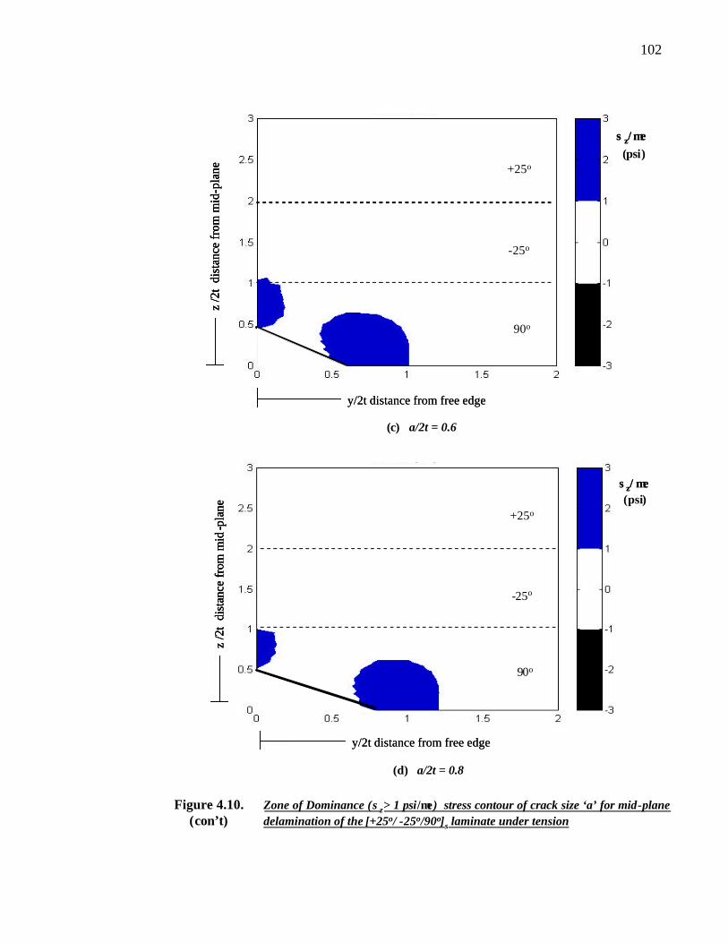
102
Figure 4.10. Zone of Dominance (σz> 1 psi/µε) stress contour of crack size ‘a’ for mid-plane (con’t) delamination of the [+25o/ -25o/90o]s laminate under tension
(c) a/2t = 0.6
y/2t distance from free edgey/2t distance from free edge
+25o
-25o
90o
z /2
t di
stan
ce fr
om m
id-p
lane
σz/ µε
+25o
-25o
90o
z /2
t di
stan
ce fr
om m
id-p
lane
z /2
t di
stan
ce fr
om m
id-p
lane
σz/ µε
y/2t distance from free edgey/2t distance from free edge
+25o
-25o
90o
z /2
t di
stan
ce fr
om m
id-p
lane
σz/ µε
+25o
-25o
90o
z /2
t di
stan
ce fr
om m
id-p
lane
z /2
t di
stan
ce fr
om m
id-p
lane
σz/ µε
(d) a/2t = 0.8
(psi)
(psi)

103
Figure 4.11. Zone of Dominance (ZOD) and average interlaminar normal stress (σz avg) as afunction of crack length for mid-plane delamination of [+25o/ -25o/90o]s laminateunder tension. σz avg. is the average over an 15 fiber diameter area around the crack-tip
0 0.5 1 1.5 2 2.5 3 3.52
2.5
3
3.5
0 0.5 1 1.5 2 2.5 3 3.550
100
150
200
ZODσz avg(psi/uε)
a/2t
σz avg
ZOD
0 0.5 1 1.5 2 2.5 3 3.52
2.5
3
3.5
0 0.5 1 1.5 2 2.5 3 3.550
100
150
200
ZODσz avg(psi/uε)
a/2t
σz avg
ZOD

104
CHAPTER 5: MICRO-STRESS FIELD ANALYSIS
The delamination model in the previous chapter is used to predict the onset and
growth of delamination provided that the effective flaw is sufficient size. While the
exact size of the flaw at delamination onset cannot be determined, it is believed that a
correlation may be found at the micro-scale where delamination is thought to originate.
At the micro-scale, the initial damage modes in the laminates are mostly in the form of
micro-cracks that develop throughout fiber, matrix material, and/or the matrix-fiber
interfaces. The micro-mechanical analysis has the advantage of providing detailed
information about these local constituents as well as the interactions among them. This
information has been previously lost in the homogenization process used at the macro-
scale of laminate analysis.
In this chapter, an attempt is made to recover the laminate micro-stresses by a
ply dehomogenization process. Emphasis is placed at the regions with high
interlaminar stress gradient zones, where delamination is most likely to occur. Analysis
of the micro-stresses within these zones then helps identify the possible micro-
mechanisms that initiate failure. A laminate case study is presented with numerical
results.

105
5.1 MACRO TO MICRO MODELING
5.1.1. Fiber/Matrix Microstructure
Ply dehomogenization is the process in which the ply microstructure is restored
from the effective ply medium. For the unidirectional ply, the microstructure consists
of the fiber and matrix materials, but may also include fiber-matrix disbands, voids and
micro-cracks in the matrix, etc. In addition, the fiber themselves can vary in size and
shape, or possibly broken or uneven in distribution. This random nature in the ply
microstructure makes modeling its true representation impractical, if not impossible.
In practice, then, the ply microstructure is often simplified using certain key
assumptions. One key assumption is that the microstructure possesses a degree of
statistical homogeneity [60]. This infers that the fiber-volume fraction, Vf, is uniform
through out the entire ply; likewise, all other effective properties like Vf are also
uniform in the ply. In reality, Vf varies from location to location if the ply is viewed
under high magnification. The local Vf depends on the size and location of the volume
in which Vf is computed [61]. Hence, Vf is shown to be uniform only when the ply is
viewed over a large region, where Vf is computed over a sufficiently large volume.
Another key assumption is that ply microstructure possesses a degree of
material symmetry. Material symmetry is generally controlled by the fabrication of the
ply such that the fiber arrangement can be made intentionally with a periodic
distribution or random distribution. The periodic fiber distribution is commonly
represented by a rectangular array or a square array, and the hexagonal array is
sometimes used to represent a random fiber distribution. Again, material symmetry
hold true only when the ply is viewed over a sufficiently large volume.

106
With the statistical homogeneity and material symmetry assumptions, the fiber
distribution has a continuous set pattern through out the ply microstructure. This not
only eases some of the difficulties in modeling the ply microstructure, but also it may
also allow a unit cell or representative volume element (RVE) to be identified within
the ply.
5.1.2. Representative Volume Element Concept
The concept of the RVE assumes that a small volume can be isolated from the
ply such that the average properties over the RVE represents the effective properties
homogenized ply. In theory, then, if the characteristics of the RVE (material properties,
Vf, material symmetry, etc.) are assumed the same as the ply, then only one RVE needs
to be analyzed in obtaining the material response of the ply.
In general, there are two types of RVEs: single fiber and multiple- fiber. In the
single fiber RVE, the ply microstructure is represented using one fiber embedded in the
matrix material. The composite-cylinder model is one such model. It uses two
cylinders or rings to represent the ply microstructure: the inner ring denotes the fiber
and the outer ring denotes the matrix material [62]. An assumed boundary condition is
prescribed on the outer surface of the matrix cylinder, and the response of RVE is
analyzed. While several variations of this model exist, a significant limitation in these
models is that the fiber-fiber interaction effects are not adequately taken into account
because only one fiber is used in the representation.
In the multiple- fiber RVE, the ply microstructure is modeled using any number
of fibers surrounded by a matrix material. The advantage of this type of RVE is that the
fiber packing, whether a periodic or random array, is explicitly defined in the RVE.

107
The periodic array model, for example, is used for a rectangular or square fiber-
packing array [63]. Under uniform loading, the stress/strain field in the ply is periodic
in nature due to the regularly packed fiber distribution in the microstructure. The RVE,
then, is modeled using one unit-cell, consisting of a fiber embedded in a rectangular or
square matrix base. Periodic boundary constraints are imposed on the RVE that is
consistent with the traction and displacement field of the neighboring unit cells. This
takes into the account the fiber-fiber interaction between unit cells. However, the
periodic array model is not intended for random fiber distributions.
Whether the single fiber or multi fiber RVE is defined, the premise for using
the RVE is the same; that is, to predict the average response of the ply (i.e. the
homogenization process). Or, in the reverse situation, the average response of the ply is
used to predict the micro- level responses of the ply; this point is crucial in this analysis.
5.1.3. Effective Ply Properties Prediction
The effective ply properties can be determined by solving the boundary value
problem of the selected RVE. Briefly, a specified boundary condition is first prescribed
on the RVE and the corresponding fiber/matrix stress and strain field is computed.
These stresses are then averaged to obtain the effective stress and strain fields of the
homogenized RVE, which in turn, yield the effective ply properties. This is a forward
approach to predict the global response of the ply. Ideally, the backward approach
should also hold true where effective stress/strains can be used to recover the micro-
stress field once the RVE is dehomogenized.
The problem in solving the boundary value problem, however, is that the
boundary conditions of the RVE are generally unknown. The boundary cond itions are,
108
in fact, the traction or displacement fields of the homogenized ply, which is part of the
RVE solution. Arbitrary or improper boundary conditions can lead to inaccurate
predictions of the effective ply properties.
One method to estimate the effective ply properties is using the bounding
method, presented by Hashin and Rosen [62]. In this method, either surface traction or
displacements are specified on the RVE boundaries. If surface tractions are specified, it
is shown that the material response of the RVE is more rigid than expected. This then
yields a lower bound estimate of the effective ply properties. On the other hand, if
displacement are specified the material response of the RVE is more flexible than
expected. This then yields an upper bound estimate of the effective ply properties.
While the bounding method is a practical means to estimate the effective ply
properties range, the dilemma remains in the micro-stress recovery. A different
effective property is obtained when either traction or displacement boundary conditions
are used. In such case, recovering the micro-stress field is not a unique process. A
model is needed that assures the response of the RVE is consistent at both the micro
and macro- level.
5.2 THE MODIFED MULTI-FIBER RVE SCHEME
Recently, a modified multi- fiber RVE model has been presented by Wang and
Yan [64]. This model appears to alleviate some of the difficulties of the RVE models
mentioned above. Unlike the previous RVE models, this model is defined with
multiple fiber elements embedded in a matrix base. Either periodic or random arrays
are possible depending on how the fibers are arranged in the RVE.
109
To illustrate, Figure 5.1 shows a schematic of modified RVE model using 12
fibers in a square fiber-packing array. In this schematic, there are four rows of fibers,
with three fibers in each row. Of the 12 fibers, only the middle two are completely
surrounded by fibers on all of its sides; they are center elements of the RVE. As the
loading is prescribed on the outer surface of the parent RVE, the response of the center
elements RVE is influenced by the surrounding fibers. Thus, the fiber- fiber interaction
effects are explicitly included in this model, without any approximations.
The center elements in the modified RVE model can be taken as an in-situ
RVE; its response is representative of the parent RVE. The distinct characteristic of the
in-situ RVE is that it is located inside the parent RVE; therefore, by Saint Venant’s
principle, any localized effects caused by the loading on the parent RVE are not
directly experienced in or near the in-situ RVE.
The advantage of the in-situ RVE is seen in the prediction of the effective ply
properties. In bounding the parent RVE, it has been shown that the effective
stress/strain state inside the in-situ RVE is the same whether a traction or displacement
boundary condition is applied, as long as they are statically equivalent. As a result, the
upper and lower bounds collapse, and only one set of effective ply properties is
yielded. The collapse bounds suggest that the computed effective ply properties are
exact or near exact. Consequently, the micro-stresses can be uniquely recovered from
the effective stress/strains field once the RVE is dehomogenized.
Another advantage of the in-situ RVE is when the RVE is situated in a singular
or stress concentration zones. In these zones, the prescribed boundary conditions are
non-uniform, where the traction and displacement distribution is nonlinear and may

110
possess sharp gradients. Regions near the surface of the parent RVE may suffer from
the loading effects, but solutions in-situ RVE should remain insensitive to the boundary
conditions.
The interaction between the stress gradient zones and the micro-stress field may
play an important role in the delamination initiation process. So far, only few have
attempted to make this connection [65-67].
5.3 MICRO-STRESS ANALYSIS
A case study is now presented to recover the laminate micro-stress field near a
high macro-stress gradient zone. In this study, the [+25o/90o]s laminate is investigated
under axial tension, ε =10-6. This laminate has been shown to delaminate at the mid-
plane due to a dominant tensile interlaminar normal stress, σz, concentration zone in
the 90o ply (see Chapter 3). For specific results, ma terial properties are taken as T300
(graphite) fibers with fiber diameter d = 0.00034 in. and an epoxy matrix material. Ply
thickness is 2t= 0.0052 in.
The effective ply properties for this laminate are computed using a modified
multi- fiber RVE homogenization scheme. The scheme assures a one to one
correspondence between the micro and macro- material responses. The particular
homogenization scheme utilized in this analysis is a 9-fiber square array RVE, where
the middle fiber is the in-situ RVE. Traction and/or displacement boundary conditions
are prescribed on the RVE, and the effective properties are predicted using only the in-
situ-RVE. This work has been performed by Yan, and details of the homogenization
process are documented in [63]. For a fiber volume fraction, Vf =56.25%, the

111
fiber/matrix material properties as well as the effective ply properties for this
composite system are given in Table 5.1.
In analyzing the micro-stress field, the first step is to compute the macro-
stresses of this laminate under the applied load. This macro-stress field provides the
boundary conditions of a selected RVE. The corresponding boundary value problem is
then solved to recover the micro-stresses.
The macro-stress field for this laminate is computed using the 3D lamination
model presented in Chapter 2. Figure 5.2 is the σz distribution along the mid-plane,
where delamination is believed to occur. It is seen that σz is tensile and has a sharp
gradient towards the free edge; maximum σz is computed to be 2.1 psi/µε. Ηere, σz is
shown with a linear increase because the plot length is relatively small in this figure,
about 5 fibers diameters into the width direction (this is the length of the micro-model,
discussed in the next section). The full stress distribution is similar to the example
shown in Figure 3.3 (a).
Figure 5.2 also shows σx distribution along the mid-plane. This stress
component is also concentrated near the free edge. σx increases rapidly towards the free
edge, with its maximum equal to 1.9 psi/µε.? However, the gradient of σx is
considerably shallower than σz. σx, in this case, remains tensile and concentrated
through out the entire 90o ply. The σx component is mainly responsible for a transverse
cracking failure mode, but is not seen in this particular laminate.

112
5.2.1 Finite Element Model
A 3D finite element analys is is used to compute the micro-stress field from the
effective stress state. To avoid modeling the entire laminate, a small section is cut away
from the macro-model, and the ply microstructure is restored at the suspected
delamination location; namely, in the laminate mid-plane region near the free edge
surface.
A 12-fiber square array RVE is used to represent the ply microstructure at the
mid-plane (see Figure 5.1). The middle two fibers are the center elements, and are the
in-situ RVE. All fibers shown here are perpendicular to free surface. Depth of the
model (into the laminate width) extends to about 5 fiber diameters, or y=0.4/2t. The
model is meshed with a finer density towards the free edge, where the edge effects are
the most dramatic. For modeling convenience, fibers are decagonal in shape. The
model is auto-meshed using 3D, 4-node tetrahedral solid elements. Solutions in this
work are rendered using the ANSYS finite element software package.
For the boundary conditions on the RVE, nodal tractions are taken from the
macro-model at the cut-out region, and in turn, are imposed on the outer surfaces of the
RVE (except for the free edge surface, which is traction free). However, the transfer of
the macro to micro boundary conditions is not a one to one correspondence since the
mesh of the micro-model is a finer mesh than the macro-model. Nodes generally do not
coincide between models, as displayed in Figure 5.3. For these nodes, the nodal
tractions are interpolated using a bi- linear interpolation function.
The corresponding boundary value problem is then solved for the RVE.
Computations are mainly limited in or near the center elements in order to avoid

113
boundary layer effects from the applied loading. To assure that the boundary conditions
have been properly transferred, Figure 5.2 also shows the σz and σx distribution of the
micro-model with the imposed nodal tractions on the RVE. Here, the stresses are
computed along the mid-plane using the effective ply properties (where the RVE is
homogenized), and are compared to the σz and σx distribution of the macro-model. The
results between the macro and the micro models are in good agreement. σz is noted to
be slightly higher at the micro-scale. This? can probably be attributed to the
approximations made from the boundary condition interpolation used at the non-
coinciding nodal points. However, this difference is small, and there is reasonable
confidence that the solutions between macro and micro models are consistent with each
other. Hence, the micro-stress field can be recovered once the RVE is dehomogenized,
where the fiber/matrix micro-structure is restored.
5.2.2 Micro- Stress Field
Figure 5.4 (a-c) and Figure 5.5 (a-b) shows the interlaminar normal stress, σz,
and axial stress, σx, distributions, respectively, of the dehomogenized RVE model
under load. These are the two dominant stress components in the macro-stress field.
Figure 5.4 (a) shows the σz stress contour across the free edge surface near the
mid-plane region. Unlike the macro-stress field, the distribution is clearly non-uniform.
While σz is constant in the fiber material (σz = 2.7 psi/µε) the ?stress varies in the matrix
material. The computed σz? in the matrix ranges from ?0.5 psi/µε to 2.7 psi/µε. σz is
largest between the vertical gaps between adjacent fibers, where local stress
concentrations exist; this are depicted in the figure as the hourglass pattern between

114
fibers (colored in yellow). In these local stress concentration zones, the magnitude of
σz is approximately the same as the fiber.
The local σz concentrations in the matrix are attributed to the fiber- fiber
interaction effect. To further illustrate this effect, Figure 5.4 (b) shows the σz
distribution along the mid-plane line, z=0 and y=0. As observed, σz oscillates; its
maximum is located exactly at the center between the adjacent fibers, σz = 2.7 psi/µε,
and its minimum at the center of non-fiber intervals, σz = 1.5 psi/µε. The average of
along this line is σz = 2.1 psi/µε, which is the about the same as the computed macro-
σz. Hence, at the extreme points, the micro-σz is considerably higher than the macro-
σz.
The stress oscillations continue to exist through the interior of the ply. Figure
5.4 (c) shows the σz distribution in the matrix along the mid-plane line, z=0, slightly
away from the free surface, y=3/2t. The stress distribution along this line is similar to
the free edge, but the average of σz and its range is lower. Here, σz varies from 1.1
psi/µε to 1.7 psi/µε and its average equal 1.4 psi/µε.? The smaller oscillations of σz
along this line suggests that the fiber interaction effect are reduced as the free edge
effects decreases.
The fiber interaction effect is also noted on the axial stress, σx, distribution.
Figure 5.5 (a) shows the σx stress contour across the free edge surface near the mid-
plane region. The distribution shown is similar to σz such local σx stress concentrations
are present in the matrix, except they are present in the horizontal gaps between
adjacent fibers (shown in yellow in the contour).σx is constant in the fiber material,
115
equal to about 2.3 psi/µε. Note that the magnitude in the stress concentration zones is
comparable to σz, where σx appears to dominant stress component in the micro-stress
field.
The fiber interaction effect on σx is illustrated Figure 5.5 (b). In this figure, the
σx distribution is plotted along ply thickness direction between adjacent fibers. σx
along this line oscillates between 1.1 to about 2.2 psi/µε, where the maximum is
located exactly at the center between the adjacent fibers, and its minimum at the center
of non-fiber intervals. The average about this line is computed at 1.6 psi/µε. This value
is slightly lower than the computed macro-σx = 1.8 psi/µε. The difference between the
values is probably attributed to the approximations made in the prescribed boundary
conditions. Still, the micro-σx is clearly higher than the macro-σz in the local stress
concentration zones in the matrix.
The fiber interaction effects can be quantified by a scaling factor, K. Here. K is
defined as the highest value, σmax, occurring in the matrix between adjacent fibers,
divided by the macro-stress, given by σave. If the fiber is stiffer than the matrix, K
should be greater than or equal to one.
Figure 5.6 shows K for the σz and σx at the mid-plane plotted against the
normalized distance from the free edge, y/2t. K is largest at the free edge, with K= 1.28
for both stress components. As y increases, K for σz is seen to decrease rapidly. It drops
to 1.2 at about 5 fiber diameters into the laminate width. It is expected that K will reach
a steady value once the edge effects has dissipated further into the laminate, and the
macro-stress state is uniform.
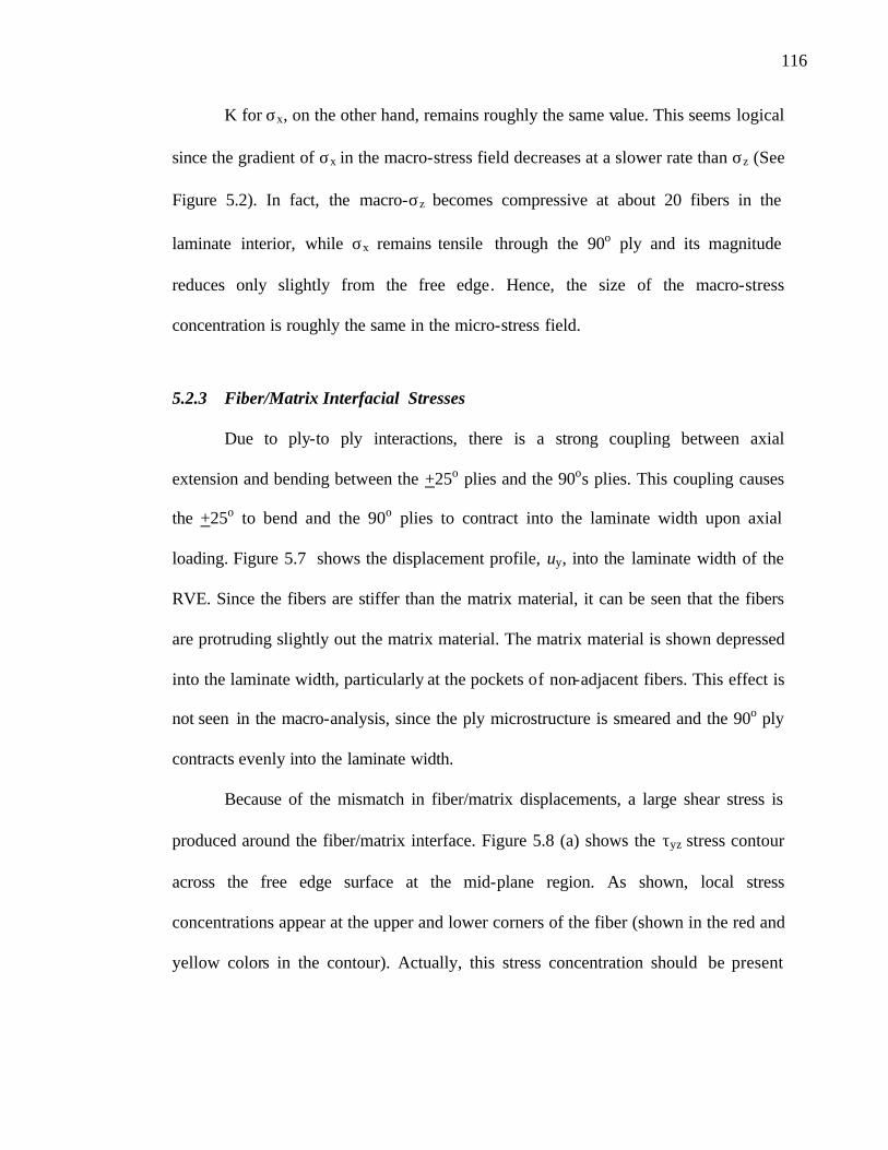
116
K for σx, on the other hand, remains roughly the same value. This seems logical
since the gradient of σx in the macro-stress field decreases at a slower rate than σz (See
Figure 5.2). In fact, the macro-σz becomes compressive at about 20 fibers in the
laminate interior, while σx remains tensile through the 90o ply and its magnitude
reduces only slightly from the free edge. Hence, the size of the macro-stress
concentration is roughly the same in the micro-stress field.
5.2.3 Fiber/Matrix Interfacial Stresses
Due to ply-to ply interactions, there is a strong coupling between axial
extension and bending between the +25o plies and the 90os plies. This coupling causes
the +25o to bend and the 90o plies to contract into the laminate width upon axial
loading. Figure 5.7 shows the displacement profile, uy, into the laminate width of the
RVE. Since the fibers are stiffer than the matrix material, it can be seen that the fibers
are protruding slightly out the matrix material. The matrix material is shown depressed
into the laminate width, particularly at the pockets of non-adjacent fibers. This effect is
not seen in the macro-analysis, since the ply microstructure is smeared and the 90o ply
contracts evenly into the laminate width.
Because of the mismatch in fiber/matrix displacements, a large shear stress is
produced around the fiber/matrix interface. Figure 5.8 (a) shows the τyz stress contour
across the free edge surface at the mid-plane region. As shown, local stress
concentrations appear at the upper and lower corners of the fiber (shown in the red and
yellow colors in the contour). Actually, this stress concentration should be present

117
around the entire fiber circumference. The stress concentrations are only seen in the
corners in this plot because of the decagonal fibers used in this model.
Figure 5.8 (b) shows τyz/µε at the fiber matrix interface plotted against the
normalized distance from the free edge, y/2t. As shown, τyz is singular at the free edge.
The strength of the singularity is computed to λ=–0.257 using the method presented in
Chapter 2. It is a relatively strong singularity compared crack tip singularity λ=–0.5. τyz
rapidly decreases to zero at about 1 fiber diameter into the laminate width. Note that
the area under the curve for +τyz appears equal to the -τyz area. This self-equilibrium
might explain why this shear stress component does not appear in the macro-analysis.
In an overall depiction, the stress field around the fiber is complex. Figure 5.9
shows a schematic of all the stresses acting at the fiber/matrix interface. It is seen that
in addition to the τyz, there is also σx and σz that pull the matrix in the axial and
transverse directions, respectively, away from the fiber. The combination of these three
stress components may contribute to local fiber/matrix disbands; or if the fiber is
already broken, fiber pull-out may also be possible. If this type of failure does occur, it
would most likely occur at the corners adjacent to neighboring fibers where σx and σz
are maximum stress due to the fiber interaction effect.
From this point of view, it is difficult to see which stress(es) will govern the
failure initiation process. The stress state in the micro-stress field is multi-dimensional.
To determine what type of failure will occur under what critical conditions would
require a specific failure criterion.

118
5.4 DISCUSSION
While the macroscopic analysis is invaluable in describing the overall response
to laminate, it is limited in describing the failure modes that may initiate delamination.
At the macro-scale, delamination is attributed mainly to presence of interlaminar stress
gradient zones, where failure is predicted using the most dominant stress component,
such as the interlaminar normal stress. However, at the micro-scale, initial cracking in
the ply may occur either in the matrix or at the fiber/matrix interface. If failure occurs
in the matrix, it would probably occur within the pockets between adjacent fibers. The
stresses in these pockets are amplified due to the fiber-fiber interaction effects. Failure
at the fiber/matrix interface, on the other hand, may be caused by several dominant
stress components. In addition to the shear stress around the fiber, a bi-axial stress at
the corners can also exist due to the fiber interaction effects. Thus, failure at this
interface can be caused by one, or a combination of these stresses.
No general working failure criterion exists for composites in the micro-scale at
this point. However, Wang and Yan [64] has recently presented a model that has
shown some success in predicting the transverse cracking behavior in composites under
compact tension. The model is essentially based on Weibull’s weakest link theory.
Briefly, the laminate is assumed composed of a number of elements arranged in a
series. Each element consists of a pair of fibers within the matrix material. The entire
laminate then is made of a chain or series of these unit-pairs. If one assumes a certain
failure probability for a given unit pair, such as a Weibull distribution as suggested the
authors, then the failure distribution can be obtained for the whole chain. Under a given

119
loading condition, one can predict whether the system will fail or not within a certain
probability.
In order to apply this model to this particular problem would require data from
specific experiments, which is beyond scope of this research. This may be a possible
direction for future research.
UD Ply : EL = 17.04 msi, Et=Ez= 0.9809 msi Glt=Glz= 0.566 msi, Gtz = 0.33 msi vlt=vlz= 0.3, vtz = 0.485
Macro-Level (Vf = 56.25%)
Graphite : EL = 29.75 msi, Et=Ez= 2.09 msi Fiber Glt=Glz= 3.4 msi, Gtz = 0.711 msi vlt=vlz= 0.27, vtz = 0.4698 Epoxy : E = 0.5 msi, G = 0.185 msi, v=0.35
Micro-Level (Fiber/Matrix)
Material Properties Scale
Table 5.1: Macro and micro-mechanical material properties of a unidirectional ply.
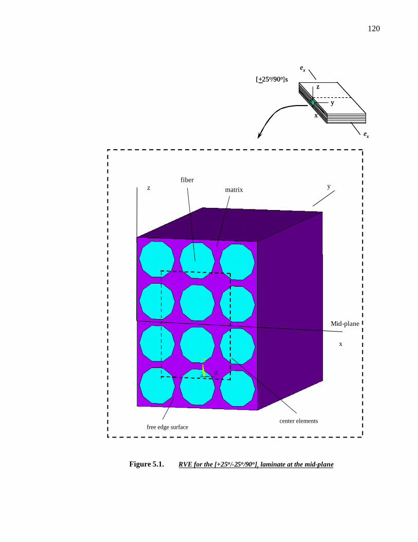
120
x
z y
z
y
x
ex
ex
[+25o/90o]sz
y
x
ex
ex
[+25o/90o]s
free edge surface
Mid-plane
fibermatrix
center elements
Figure 5.1. RVE for the [+25o/-25o/90o]s laminate at the mid-plane

121
Figure 5.2. Axial (σx) and Interlaminar normal (σz) stress distributions of the macro and micro-mechanical models along the mid-plane for [+25o/-25o/90o]s under tension
90o
90o
zy
x
z
y
x
(a) macro-mechanical FEA model (cut-out) (b) micro-mechanical FEA model
Figure 5.3. Macro and macro-mechanical FEA models used for the micro-stress recovery scheme
mid-plane 90o
90o
zy
x
z
y
x
z
y
x
(a) macro-mechanical FEA model (cut-out) (b) micro-mechanical FEA model
Figure 5.3. Macro and macro-mechanical FEA models used for the micro-stress recovery scheme
mid-plane
σzz/ue (psi)
1
1.1
1.2
1.3
1.4
1.5
1.6
1.7
1.8
1.9
2
2.1
2.2
2.3
0 0.05 0.1 0.15 0.2 0.25 0.3 0.35 0.4 0.45
Szz - Micro (homo)
Szz - Macro
Sxx - Micro (homo)
Sxx - Macro
σ /µε (psi)
y/2t
σzz/ue (psi)
1
1.1
1.2
1.3
1.4
1.5
1.6
1.7
1.8
1.9
2
2.1
2.2
2.3
0 0.05 0.1 0.15 0.2 0.25 0.3 0.35 0.4 0.45
Szz - Micro (homo)
Szz - Macro
Sxx - Micro (homo)
Sxx - Macro
σ /µε (psi)
y/2t

122
(a). σz/µε stress contour at the free surface
Figure 5.4. Interlaminar normal stress profile at the mid-plane for [+25o/-25o/90o]s laminate under tension
(b). σz stress distribution between fibers at y/2t =0
0.47530.76421.05311.34191.63081.91982.20862.49752.78643.0753
psi(mid-plane)
1
1.2
1.4
1.6
1.8
2
2.2
2.4
2.6
2.8
3
3.2
micro
macro
x/2t
σz / µε (psi)
1
1.2
1.4
1.6
1.8
2
2.2
2.4
2.6
2.8
3
3.2
micro
macro
x/2t
σz / µε (psi)

123
Figure 5.4. Interlaminar normal stress profile at the mid-plane for [+25o/-25o/90o]s(con’t) laminate under tension
(c). σz stress distribution between fibers at y/2t =0.3
0.8
0.9
1
1.1
1.2
1.3
1.4
1.5
1.6
1.7
1.8
1.9
2
micro
macro
x/2t
σz / µε (psi)
0.8
0.9
1
1.1
1.2
1.3
1.4
1.5
1.6
1.7
1.8
1.9
2
micro
macro
x/2t
σz / µε (psi)
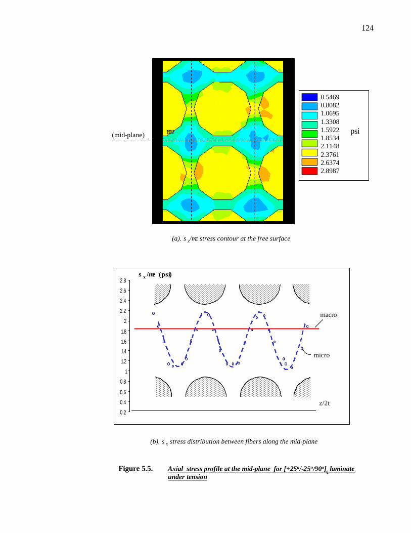
124
(a). σx/µε stress contour at the free surface
Figure 5.5. Axial stress profile at the mid-plane for [+25o/-25o/90o]s laminate under tension
(b). σx stress distribution between fibers along the mid-plane
0.54690.80821.06951.33081.59221.85342.11482.37612.63742.8987
psi(mid-plane)
0.2
0.4
0.6
0.8
1
1.2
1.4
1.6
1.8
2
2.2
2.4
2.6
2.8
z/2t
micro
macro
σx /µε (psi)
0.2
0.4
0.6
0.8
1
1.2
1.4
1.6
1.8
2
2.2
2.4
2.6
2.8
z/2t
micro
macro
σx /µε (psi)

125
1.15
1.17
1.19
1.21
1.23
1.25
1.27
1.29
0 0.05 0.1 0.15 0.2 0.25 0.3 0.35 0.4 0.45
y/2t
K
σz (Int. normal)
σx (axial)
1.15
1.17
1.19
1.21
1.23
1.25
1.27
1.29
0 0.05 0.1 0.15 0.2 0.25 0.3 0.35 0.4 0.45
y/2t
K
σz (Int. normal)
σx (axial)
Figure 5.6. Scaling factor K for the axial and interlaminar normal stresses plotted alongthe mid-plane for the [+25o/-25o/90o]s laminate
Figure 5.7. Transverse displacement profile at the mid-plane across the free edge for [+25o/-25o/90o]sunder tension
uy
0.0000000.0002380.0005310.0007150.0009530.0011720.0014300.0016690.001907
in(mid-plane)

126
(a). τyzµε stress contour at the free surface
Figure 5.8. Interlaminar shear stress profile at the mid-plane for [+25o/-25o/90o]s laminate under tension
(b). τyz stress distribution along the fiber/matrix interface
-0.5809-0.4101-0.2394-0.06870.10450.27280.44350.61420.7850
psi(mid-plane)
-0.05
0
0.05
0.1
0.15
0.2
0.25
0.3
0 0.1 0.2 0.3 0.4
y/2t
τyz/µε (psi) z
y
fiber
fiber
free edge
-0.05
0
0.05
0.1
0.15
0.2
0.25
0.3
0 0.1 0.2 0.3 0.4
y/2t
τyz/µε (psi) z
y
fiber
fiber
free edge
z
y
fiber
fiber
free edge

127
σz
σx
τyz σy
σz
σx
τyz σy
Figure 5.9. Schematic of the stress distribution around a fiber in the 90o ply for the[+25o/-25o/90o]s laminate under tension

128
CHAPTER 6: SUMMARY AND CONCLUSIONS
6.1. SUMMARY/CONCLUSIONS
The effects of interlaminar stress gradient zones have been investigated on the
free edge delamination process in the [+θο/90on]s laminate series. In this thesis, two key
issues are addressed: 1) identifying the physical sources for delamination, and 2)
establishing a physical criterion for the onset and growth of delamination. Figure 6.1
outlines the general methodology used in this thesis to compute and evaluate the edge
stress field in this series. The method is separated into three major steps: modeling,
computation, and analysis.
In the modeling step, the traditional approach is followed where the laminate is
modeled at the macroscopic scale. At this scale, the fiber/matrix microstructure in each
ply is replaced with an equivalent homogenized medium. The effective ply properties
are then used to compute the global response of the laminate under load. One result of
the smearing, or homogenization, process is the creation of artificial interfaces between
adjacent plies. A stress singularity appears at the interfaces of dissimilar materials near
the free edges. Stresses become unbounded at these locations, and therefore require
rigorous treatment in the stress computation.
In the computation step, a numerical technique is presented to obtain an
accurate, complete laminate stress field within the premise of three-dimensional
elasticity. Accuracy issues concerning the edge singularity are resolved by employing a
local-global stress matching method. A local stress solution is obtained near the
singular region by using complex variable stress potential theory in conjunction with

129
an eigenvalue expansion procedure. The local stress field is computed within a scaling
factor K that depends on the applied loading and remote boundary conditions. A global
stress solution is obtained by a finite element analysis of the entire laminate. K is then
computed by matching the angular variation of both the local and global solutions
within a small zone near the free edge. With the computed K, the two solutions are
combined to provide the full laminate stress field.
The stress matching zone is shown to depend highly on the strength of the
singularity, λ. For the graphite-epoxy laminates studied here, λ is shown to be weak
(generally an order of magnitude smaller than λ in elastic crack tip problems). A larger
scaling factor K is needed for smaller values of λ. The matching zone is estimated to
occur within one fiber diameter from the free edge in these laminates. In such case, a
successful matching is not realistic since the matching zone is essential zero. This
suggests that the singular stress solution is confined to the immediate region near the
free edge. The finite element analysis, therefore, appears sufficient in characterizing the
complete laminate stress field, including the singular region, for all practical purposes.
With the obtained full field laminate stress field, the effects of the singularity
are then weighed against other sources that contribute to high interlaminar stresses.
Two key lamination parameters in the [+θο/90on]s laminate series, specifically the ply
fiber orientation (θ) and 90o ply thickness (n), are varied and changes in the laminate
stress field are observed. While edge singularities exist at the +θο and the -θο/90o
interface, a large interlaminar normal stress, σz, concentration also exists in the 90o ply
when a tensile load is applied. The stress concentration is caused by the mismatch in
poisson ratio between the grouped +θο plies and the 90no ply.
130
It is observed that stress distribution in the singular zones remain unchanged
with the variations in the θ and n parameters; however, size of the stress concentration
zone, or zone of dominance (ZOD), becomes considerably large when either the
poisson mismatch between the grouped +θο plies or the 90no ply is increased or the
thickness of the 90no plies are increased . The ZOD of the edge singularities is small
due to weak singularity strengths. Hence, ZOD of the stress concentration zone can be
significantly larger than the singular stress zones.
Edge delamination is shown to coincide at location with the largest zone of
dominance rather than at the point of highest stress magnitude. In this regard, the ZOD
seems to have a larger influence on the delamination process than the actual magnitude
of the stress at the free edge. In situations where the singularity can coincide with stress
concentrations, it is unknown if the former enhances the effects of the latter.
In third step, analysis, an attempt is made to incorporate the computed edge
stresses into a failure model to predict the onset and growth of delamination. In this
thesis, a failure model based on the effective flaw concept is employed. The effective
flaw concept is an inexact, but necessary, means to represent the effects of the
randomly distributed micro-cracks in the laminate. The assumed effective flaw is
treated as a physical crack that propagates uniformly towards the center of the
laminate, assuming delamination is the only failure event during the course of loading
(i.e. no transverse cracking, fiber breakage, etc).
The criterion for crack growth is then provided by the theory of fracture
mechanics. The energy release rate of the propagating crack is measured against the
material fracture toughness. The driving force for crack growth is provided by the

131
energy stored in the crack-tip concentration zone. In investigating the poison mismatch
effect, results showed that laminates with a higher poisson mismatch between the
+θο and the 90no plies produced a larger ZOD at the laminate mid-plane. These
laminates tend to release more energy during crack growth, and therefore appeared to
be more energetically favorable for delamination. The predicted delamination onset
strain was shown to match well with the observed onset strain when thermal residual
stresses are included in the computations.
On the other hand, the thickness effect investigation showed that thicker 90no
ply laminates produced a larger ZOD at the laminate mid-plane, but generally released
less energy during crack growth. This suggests that the thicker 90no ply laminates are
less likely to delaminate, at least as its first mode of failure. This coincides with the
observance of transverse cracking prior to delamination in these laminates. The
presence of transverse cracks can lower the delamination onset strain prediction. To
predict failure in these laminates, a separate analysis for transverse cracking has to be
performed.
While the effective flaw is an essential feature in the above model, the exact
size of the flaw could not be determined. The model can only predict the minimum
critical load for onset, based when the energy release rate of the flaw is stable and
delamination is already fully developed. The minimum flaw size is generally on the
order of one to two ply thicknesses for the graphite-epoxy laminate examined. To
determine the size of the effective flaw, it is believed that a correlation may be found at
the fiber/matrix scale where delamination is thought to originate.
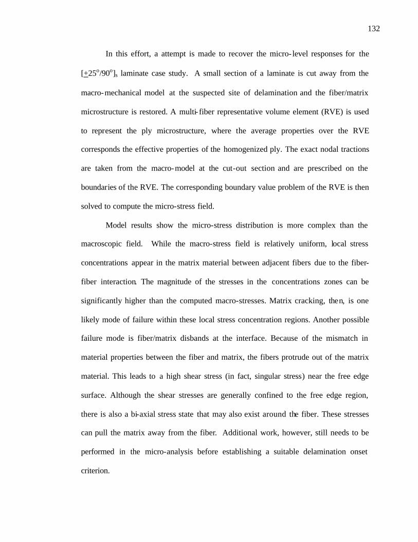
132
In this effort, a attempt is made to recover the micro- level responses for the
[+25ο/90o]s laminate case study. A small section of a laminate is cut away from the
macro-mechanical model at the suspected site of delamination and the fiber/matrix
microstructure is restored. A multi- fiber representative volume element (RVE) is used
to represent the ply microstructure, where the average properties over the RVE
corresponds the effective properties of the homogenized ply. The exact nodal tractions
are taken from the macro-model at the cut-out section and are prescribed on the
boundaries of the RVE. The corresponding boundary value problem of the RVE is then
solved to compute the micro-stress field.
Model results show the micro-stress distribution is more complex than the
macroscopic field. While the macro-stress field is relatively uniform, local stress
concentrations appear in the matrix material between adjacent fibers due to the fiber-
fiber interaction. The magnitude of the stresses in the concentrations zones can be
significantly higher than the computed macro-stresses. Matrix cracking, then, is one
likely mode of failure within these local stress concentration regions. Another possible
failure mode is fiber/matrix disbands at the interface. Because of the mismatch in
material properties between the fiber and matrix, the fibers protrude out of the matrix
material. This leads to a high shear stress (in fact, singular stress) near the free edge
surface. Although the shear stresses are generally confined to the free edge region,
there is also a bi-axial stress state that may also exist around the fiber. These stresses
can pull the matrix away from the fiber. Additional work, however, still needs to be
performed in the micro-analysis before establishing a suitable delamination onset
criterion.

133
6.2 DIRECTIONS FOR FUTURE WORK Although the macro- level response of composite laminates is reasonable well
understood, the micro-mechanical laminate stress analysis is a relatively new research
field. The micro-mechanical laminate model presented in this thesis is a simple tool
that bridges the gap between the macro and micro-scales. One consideration not
examined in this study is the effects of laminate residual thermal stresses on the micro-
stress field. These stresses have been shown to significantly influence the delamination
failure process such that fa ilure is computed at a lower predicted strain when these
stresses were included in macro-failure models. Another consideration that not
included in this micro-stress analysis is different bonding conditions of the fiber and
matrix. Bonding is assumed perfect in this thesis, but a more realistic simulation might
include cracked interfaces. Addition of micro-flaws into the matrix material is also a
possibility.
Also, although this thesis is concentrated on free edge delamination, it is
observed the close competing effects from other damage modes, particularly as
transverse cracking for the laminates studied. The study of interacting effects among
transverse cracking, delamination, and other final failure mechanisms may be an
essential feature in the laminate failure analysis.
And finally, a complete simulation of the micro-failure mechanisms has not
been performed largely due to the lack of a general failure criterion. To do so requires
specific experimental results to ascertain the critical stress values for the particular
laminate investigated. A recent failure model presented by Wang and Yan [64] has
shown some promise in this field. The method considers the fiber effects on the micro-

134
laminate stress field and is able to incorporate them into a statistical failure model.
Future research might include how to integrate the analysis in this research with Wang
and Yan failure model.

135
a
1. L
amin
ate
Mod
elin
g :
Lam
inat
e un
der
uni-
axia
l lo
adin
g
2.
Fre
e E
dge
Stre
ss A
naly
sis:
Stre
ss-m
atch
ing
tech
niqu
e fo
rhi
gh s
tress
gra
dien
t zon
es(s
ingu
lar o
r stre
ss
conc
entr
atio
n)
3. D
elam
inat
ion
Pre
dict
ion
:
Frac
ture
Mec
hani
cs A
ppro
ach
(Ene
rgy
rele
ase
rate
cri
teri
a)
3.
Del
amin
atio
n In
itia
tion
:
Mic
ro-m
echa
nica
l A
ppro
ach
(Fib
er/M
atri
x re
stor
ed)
Figu
re 6
.1:
Gen
eral
met
hodo
logy
to s
tudy
the
effe
cts
of in
terl
amin
ar s
tres
s gr
adie
nt z
ones
on
the
free
edg
e de
lam
inat
ion
prob
lem
in
com
posi
te la
min
ates
.
a
1. L
amin
ate
Mod
elin
g :
Lam
inat
e un
der
uni-
axia
l lo
adin
g
2.
Fre
e E
dge
Stre
ss A
naly
sis:
Stre
ss-m
atch
ing
tech
niqu
e fo
rhi
gh s
tress
gra
dien
t zon
es(s
ingu
lar o
r stre
ss
conc
entr
atio
n)
3. D
elam
inat
ion
Pre
dict
ion
:
Frac
ture
Mec
hani
cs A
ppro
ach
(Ene
rgy
rele
ase
rate
cri
teri
a)
3.
Del
amin
atio
n In
itia
tion
:
Mic
ro-m
echa
nica
l A
ppro
ach
(Fib
er/M
atri
x re
stor
ed)
aa
1. L
amin
ate
Mod
elin
g :
Lam
inat
e un
der
uni-
axia
l lo
adin
g
2.
Fre
e E
dge
Stre
ss A
naly
sis:
Stre
ss-m
atch
ing
tech
niqu
e fo
rhi
gh s
tress
gra
dien
t zon
es(s
ingu
lar o
r stre
ss
conc
entr
atio
n)
3. D
elam
inat
ion
Pre
dict
ion
:
Frac
ture
Mec
hani
cs A
ppro
ach
(Ene
rgy
rele
ase
rate
cri
teri
a)
3.
Del
amin
atio
n In
itia
tion
:
Mic
ro-m
echa
nica
l A
ppro
ach
(Fib
er/M
atri
x re
stor
ed)
Figu
re 6
.1:
Gen
eral
met
hodo
logy
to s
tudy
the
effe
cts
of in
terl
amin
ar s
tres
s gr
adie
nt z
ones
on
the
free
edg
e de
lam
inat
ion
prob
lem
in
com
posi
te la
min
ates
.
136
List Of References 1. Wilkins, D.J., et al., “Characterizing Delamination Growth in graphite-Epoxy,”
Damage in Composite Materials, STP 775, K. Reifnider, Ed., American Society for Testing and Materials, 1982.
2. Foye, R.L. and Baker, D.J., “Design of Orthotropic Laminates,” presented at the 11th Annual AIAA Structures, Structural Dynamics, and Materials Conference, Denver, Colorado, April 1970. 3. Wang, A.S.D., “Fracture Analysis of Interlaminar Cracking,” Interlaminar Responses of Composite Materials : Composite Materials Series: Vol 5, N.J. Pagano (editor), Elsevier, Amsterdam, Netherlands, 1989, pg. 69. 4. Bjeletich, J.G., Crossman, F.W. and Warren, W.J., “The Influence of Stacking
Sequence on Failure Modes in Quasi-Isotropic Graphite-Epoxy Laminates,” Failure Modes in Composites –IV, J.R. Cornie and F.W.Crossman (editors), American Institute of Mining, Metallurgical and Petroleum Engineers, New York, NY, 1979, pg. 118.
5. Reifsnider, K.L., Henneke, E.G. and Stinchcomb, “Delamination in Quasi-
Isotropic Graphite-Epoxy Laminates,” Composite Materials: Testing and Design, ASTM STP 617, 1977, pg. 93.
6. Rodini, B.T. and Eisenmann, “An Analytical and Experimental Investigation of
Edge Delamination in Composite Laminates,” Fibrous Composites in Structural Design, E.M. Lenoe, D.W. Oplinger and J.J.Burke (editors), Plenum Press, NY, 1978, pg. 441.
7. Crossman, F.W. and Wang, A.S.D ., “The Dependence of Transverse Cracking
and Delamination on Ply Thickness in Graphite-Epoxy Laminates,” Damage in Composite Materials, ASTM-STP-775, K.L.Reifsnider (editor), 1982, pg. 118.
8. Hashin, A. “Analysis of Properties of Fiber Composites with Anistropic
Constituents,” Journal of Applied Mechanics, Vol 46, 1979, pg. 543. 9. Stavsky, Y., Proc Amer. Soc. Civil. Eng. J. Eng. Mech. Div., Vol 87, 1900, pg. 31. 10. Dong, S.B., Pister, K.S., and Taylor, R.L., Journal of Aerospace Science, Vol 29, 1962, pg. 969. 11. Aston, J.E. and Whitney, J.M., Theory of Laminated Plates, Technomic, Westport, CT.
137
12. Hayashi, T., “Analytical Study of Interlaminar Shear Stresses in a Laminate Composite Plate,” Trans. Jpn. Aeron & Space Sci., Vol 10, 1967, pg.43 13. Puppo, A.H. and Evensen, H.A., “Interlaminar Shear in Laminated Composites
under Generalized Plane Stress,” Journal of Composite Materials, Vol 4, 1970, pg. 204.
14. Pagano, N.J. and Pipes, R.B., “Interlaminar Stresses in Composite Laminates Under Uniform Axial Extension,” Journal of Composite Materials, Vol 4, 1970, pg. 538.
15. Pagano, N.J. and Pipes, R.B., “Some Observations on the Interlaminar Strength
of Composite Laminates,” International Journal of Mechanic Science, Vol 15, 1973, pg. 679.
16. Pagano, N.J. and Pipes, R.B., “The Influence of Stacking Sequence on Laminate Strength,” Journal of Composite Material, Vol 5, 1971, pg.50. 17. Hsu, P.W., “Interlaminar Stresses in Composite Laminates – A Perturbation Analysis,” Ph.D. Thesis, VPI and SU, 1976. 18. Whitney, J.M. and Sun, C.T., “A Higher Order Theory for Extensional Motion of Laminated Composites,” Journal of Sound and Vibration, Vol 30, 1973, pg. 85. 19. Tang, S. and Levy, A., “A Boundary Layer Theory- Part II: Extension of
Laminated Finite Strip,” Journal of Composite Materials, Vol 9, 1975, pg. 668.
20. Pagano, N.J., “Stress Fields in Composite Laminates,” International Journal of
Solid Structures, Vol 14, 1978, pg.385. 21. Wang, A.S.D and Crossman, F.W., “Some New Results on Edge Effects in
Symmetric Composite Laminates,” Journal of Composite Materials, Vol 11, 1977, pg. 92.
22. Law, G.E. Fracture Analysis of (+25/90n)s Graphite-Epoxy Composite
Laminates, PhD Thesis, Drexel University, 1981. 23. Rybicki, E.F., “Approximate Three-Dimensional Solutions for Symmetric Laminates Under In-plane Loading,” Journal of Composite Materials, Vol 5, 1971, pg. 354. 24. Stanton, E.L., Crain, L.M.and Neu, T.F., “A Parametric Cubic Modeling for General Solids of Composite Materials,” Int. Journal. Num. Meth. Eng, Vol 11, 1977, pg. 653.
138
25. Hwang, W.C. and Sun, C.T., “Analysis of Interlaminar Stresses Near Curved Free Edges of Laminated Composites using Iterative Finite Element Method,” Computers and Structures, Vol 28, 1988, pg. 461.
26. Murphy, P.L.N. and Chamis, C.C., “Free Edge Delamination:Laminate width
and loading conditions effects,” Journal of Composites Tech & Research, Vol 11, 1989, pg. 15.
27. Yang, H. and He, C.C., “Three Dimensional Finite Element Analysis of the
Free Edge Stresses of Composite Laminates,” Journal of Composite Materials, Vol 28, 1994, pg. 1394.
28. Wang, S. S. and Choi, I., “Boundary-Layer Effects in Composite Laminates – 1. Free Edge Singularities,” Journal of Applied Mechanics, Vol 49, 1982, pg. 549. 29. Wang, S. S. and Choi, I., “Boundary-Layer Effects in Composite Laminates – 2. Free Edge Stress Solutions and Basic Characteristics,” Journal of Applied Mechanics, Vol 49, 1982, pg. 541. 30. Wang, S.S. and Yuan, F.G., “A Hybrid Finite Element Approach to Composite Laminate Elasticity Problems with Singularities,” Journal of Applied Mechanics, Vol 50, 1983, pg. 835. 31. Tong, P. and Pian, T.H.H., “On the Convergence of Finite Element Method for
Problems with Singularity,” International Journal of Solids and Structures, Vol 9, 1973, pg.313.
32. Bar-Yoseph, P. and Ben-David, D., “On Mesh Refinement Methods of Mixed-
Hybrid Elements for Revealing the Nature of Singularity in the Free Edge of a Composite Laminated Plate,” Communications in Applied Numerical Methods, Vol 7, 1991, pg. 315.
33. Pagano, N.J. and Soni, S.R., “Models for Studying Free-edge Effects,”
Interlaminar Responses of Composite Materials : Composite Materials Series: Vol 5, N.J. Pagano (editor), Elsevier, Amsterdam, Netherlands, 1989, pg. 1.
34. Yin, W.L., “A General Analysis Method for Singularities in Composite
Structures,” Proceedings of 1997 38th AIAA/ASME/AHS/ASC Structures, Structural Dynamics & Materials Conference. Part 3 (of 4), April 7-10,1997, Kissimmee, FL,USA, pg.2238-2246.
35. Feng, W. and Hoa, S., “3-D global/local model using partial hybrid elements
and its software COMSA for Composite Analysis,” Proceedings of the International Conference on Computer Methods in Composite Materials, CADCOMP, 1998, Montreal, Canada.

139
36. Becker, W., “Closed Form Solution for the Free Edge Effect in Cross Ply Laminates,” Composite Structures, Vol 26, 1993, pg. 39.
37. Han, Y. and Kumosa, M., “Adhesively Bonded Composite Iosipescu
Specimens without Singular Stress Fields,” Mechanics of Composite Materials and Structures: An International Journal, J.N. Reddy (Editor), Vol 5, No.2, 1998, pg.127-151.
38. Azzi, V.O. and Tsai, S.W., “Anisotropic Strength of Composites,” Experimenta lMechanics, Vol 5, 1965, pg. 283. 39. Hill, R., “A Theory of the Yielding and Plastic Flow of Anisotropic Metals,” A Proceedings of the Royal Society, Vol 193, 1948, pg 281 40. Tsai, S.W. and Wu, E.M., “A General Theory of Strength for Orthotropic Materials,” Journal of Composite Materials, Vol 5, 1971, pg. 58. 41. Whitney, J.M. and Nuismer, R.J., “Stress Fracture Criteria for Laminated
Composites Containing Stress Concentrations,” Journal of Composite Materials, Vol 8, 1974, pg. 253.
42. Hinton, M.J. and Soden, P.D., “Predicting failure in Composite Laminates,”
Composite Science and Technologies, Vol 58, 1998, pg.1001. 43. Wang, A.S.D. and Crossman, F.W., “Initiation and Growth of Transverse Cracks and Edge Delamination in Composite Materials : Part 1. An Energy Method,” Journal of Composite Materials, Vol 14, 1980, pg. 71 44. Crossman, F.W., Warren, W.J., Wang, A.S.D. and Law, G.E. "Initiation and
Growth of Transverse Cracks and Edge Delamination in Composite Laminates, Part 2: Experimental Correlation," Jour. Composite materials, Vol. 14, 1980, pg. 88-108.
45. Lekhnitskii, S. G., Theory of Elasticity of an Anisotropic Body, Holden-Day, San Francisco, CA, 1963. 46. Jones, R.M., Mechanics of Composite Materials, Taylor and Francis, Inc, Edward Brothers, Ann Arbor, MI, 1998. 47. Pochiraju, K., Mechanics of the Single Fiber Pullout Problem With Several Interface Conditions, Ph.D. Thesis, Drexel University, 1993. 48. Bogy, D.B., “Two Edge Bonded Elastic Wedges of Different Materials and Wedge Angles under Surface Tractions,” Journal of Applied Mechanics, Vol 93, 1971, pg. 377.

140
49. Hein, V.L. and Erdogan, F. Stress singularities in a Two Material Wedge, International Journal of Fracture Mechanics, Vol 7 (3), 1971, pg. 317. 50. Williams, M.L., “Stress Singularities resulting from Various Boundary Conditions at Angular Corners of Plates in Extension”, Journal of Applied Mechanics, Vol 74, 1952, pg. 526. 51. Williams, M.L., “The Stresses around a Fault or Crack in Dissimilar Media,” Bulletin of Seismological Society of America, Vol 49 (2), 1959, p. 199 52. Zak, A.R. and Williams, M.L., “Crack Point Singularities at Bi-Material Interface,” Journal of Applied Mechanics, Vol 30, 1960, pg 142. 53. Pochiraju, K., Lau, A.C.W. and Wang, A.S.D., “Analysis of Fiber Pullout or
Push- in with Frictional Sliding at the Fiber-Matrix,” Journal of Applied Mechanics, Vol 30, 1960, pg 142.
54. Kim, R.Y., “Experimental Observations of Free-Edge Delamination,” Interlaminar Responses of Composite Materials : Composite Materials Series: Vol 5, edt. N.J. Pagano, Elsevier, Amsterdam, Netherlands, 1989, pg. 111. 55. Griffith,A.A., “The Phenomenon of Rupture and Flow in Solids,” Philosophical Transactions, Series A. 221, 1920, pg.163. 56. Wang, A.S.D., “Fracture Mechanics of Sublaminate Cracks in Composite Materials,” Composite Technology Review, ASTM, 1984, Philadelphia, PA, pg. 45-61. 57. Irwin, G.R., “Fracture,” Handbuch der Physik, , Springerverlag, Vol. 5, 1958, pg. 551. 58. Crossman, F.W., Warren, W.J., Wang, A.S.D., and Law, G.E., “Initiation and Growth of Transverse Cracks and Edge Delamination In Composite Laminates,” Journal of Composite Materials, Vol 18, 1984, pg.239. 59. Wang, A.S.D., Kishore, N.N. and Li, C.A., “Crack Development in Graphite- Epoxy Cross-ply Laminates under Uni-Axial Tension,” Composite Science and Technology, Vol 24, 1985, pg.1 -31. 60. Hill, R., “Theory of Mechanical Properties of Fiber-Strengthened Materials:I. Elastic Behavior,” Journal of Mech. Phys. Solids, Vol 12, 1964, pg. 199-212. 61. Wang, A.S.D. and Yan, C., “On Composite Homogenization Theory,” Proc. of ICCM 13, Beijing, 2001.
141
62. Hashin, Z. and Rosen, B.W., “The Elastic Moduli of Fiber-Reinforced Materials,” Journal of Applied Mechanics,” 1964, pg. 223-232. 63. Pagano, N.J. and Yuan, F.G., “ Elastic Moduli of Brittle Matrix Composites with Interfacial Debonding,” International Journal of Solids and Structures, Vol 34, 1997, pg. 177-201.
64. Yan, C., Homogenization and the De-homogenization in Composite Materials, Ph.D. Thesis, Drexel University, 2003 65. Pagano, N.J. and Yuan, F.G., “ The Significance of Effective Modulus Theory (homogenization) in Composite Laminate Mechanics,” Composite Science and Technologies, Vol 60, 2000, pg. 2471-2488. 66. Hutapea, P., Yuan, F.G. and Pagano, N.J, “ Micro-stress Prediction in Composite Laminates with High Stress Gradients,” International Journal of Solids and Structures, Vol 40, 2003, pg. 2215-2248. 67. Ellyin, F., Xia, Z., and Chen, Y., “Viscoelastic Micromechanical Modeling of
Free Edge and Time Effects in Glass Fiber/Epoxy Cross-Ply Laminates,” Composites: Part A, Vol 33, 2002, pg. 399-409.
68. Rybicki, E.F. and Kanninen, M.F., “ A Finite Element Calculation of Stress Intensity Factors by a Modified Crack Closure Integral,” Engineering Fracture Mechanics, Vol. 9, 1977, pg.931.
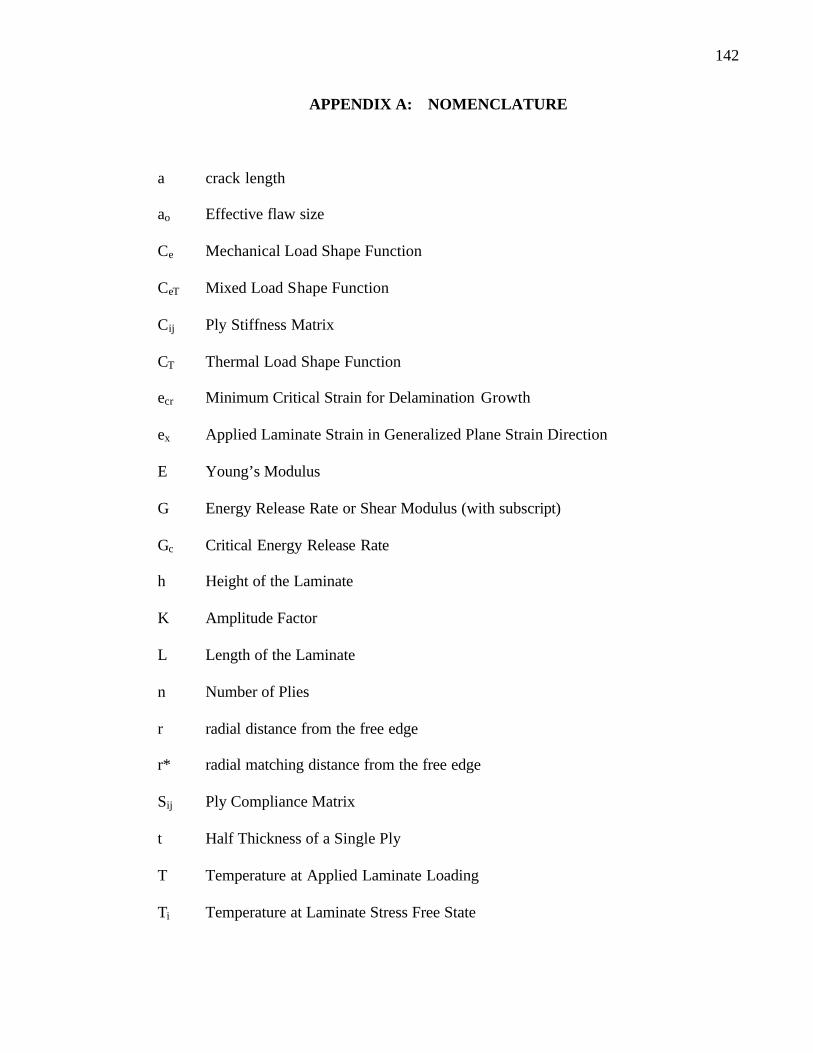
142
APPENDIX A: NOMENCLATURE
a crack length
ao Effective flaw size
Ce Mechanical Load Shape Function
CeT Mixed Load Shape Function
Cij Ply Stiffness Matrix
CT Thermal Load Shape Function
ecr Minimum Critical Strain for Delamination Growth
ex Applied Laminate Strain in Generalized Plane Strain Direction
E Young’s Modulus
G Energy Release Rate or Shear Modulus (with subscript)
Gc Critical Energy Release Rate
h Height of the Laminate
K Amplitude Factor
L Length of the Laminate
n Number of Plies
r radial distance from the free edge
r* radial matching distance from the free edge
Sij Ply Compliance Matrix
t Half Thickness of a Single Ply
T Temperature at Applied Laminate Loading
Ti Temperature at Laminate Stress Free State

143
u Displacement in the x-direction
v Displacement in the y-direction
w Displacement in the z-direction
W Width of the Laminate
ZOD Zone of Dominance
∆a Incremental Crack Extension
∆T Thermal Load
α Thermal Expansion Coefficient
ε Normal Strain
γ Shear Strain
λ Singularity Strength
ν poisson ratio
σ Normal Stress
σ?ij Angular Stress Variation
τ Shear Stress
θ Angle
I (subscript) Mode I Crack Growth
II (subscrip t) Mode II Crack Growth
III (subscript) Mode III Crack Growth
L (subscript) Longitudinal Direction
T (subscript) Transverse Direction
z (subscript) Thickness Direction

144
APPENDIX B: PLY STIFFNESS ROTATION This appendix outlines the stiffness transformation for a unidirectional laminate
ply. The principle coordinate system for a given ply is defined as Y = [L T z] where the
fibers are aligned with the longitudinal direction (L), (T) transverse to the fibers, and
(z) through the thickness of the ply. The transformed coordinate system is designated
as Y’ = [1 2 3] directions, as shown in the figure below. Here, a special rotation is
considered in the 1-2 plane about the common z (3)-axis. The amount of rotation is
denoted by the angle θ, where θ is measured positive counterclockwise from the L-axis
to the 1-axis.
Figure A.1. Axis rotation for a uni-directional fiber-reinforced ply
For the special rotation, (L,T,z) coordinate system can be expressed in the (1,2,3)
coordinate system by introducing directional cosines, aij, between the two sets of axes:
z,3
1
2
T
L
θ

145
m2–n2 0 0 0 mn -mn
0 m n 0 0 0
0 -n m 0 0 0
0 0 0 1 0 0
-2mn 0 0 0 m2 n2
2mn 0 0 0 n2 m2
= T1
σijp T1 σij =
a =
a11 a12
a13
a21
a22
a23
a31
a32
a33
cos(θ)
=
sin(θ) 0
-sin(θ) cos(θ) 0
0 0 1
σ ijp a σij = a -1
[Y] = [a] [Y’] (A.1) where
(A.2)
Note that the transformation matrix a is asymmetric, and the direction of rotation is
important.
The stress components, {σij}, (i =1,2,3), are second order tensors. Therefore,
{σijp} in the principle coordinate system can be rotated to {σij} in the 1,2, 3 coordinate
system by using the tensor transformation law:
(A.3) or,
(A.4) where [T1] is
(A.5)

146
ε ijp T2 ε ij =
σijp Cij
p ε ijp
=
σij Cij p ε ij = T1 T2
σij Cij p ε ij = T2 T1
-1
σij Ci j ε ij =
m2–n2 0 0 0 2mn -2mn
0 m n 0 0 0
0 -n m 0 0 0
0 0 0 1 0 0
-mn 0 0 0 m2 n2
mn 0 0 0 n2 m2
= T2
and m = cos(θ) and n = sin(θ). The superscript p denotes the principle coordinate
system (L,t,z), and the standard notation (no superscript) represents the transformed
coordinate system.
The strain components, {ε ij}, can be transformed in a similar fashion.
(A.6)
where [T2] is
(A.7)
Note that transformation [T] for strain is the not the same for stress because of the
engineering shearing strains are used. The transformation of the stiffness matrix, [C ij]
can be performed by substituting the above relations into the ply constitutive equation
Eq. (2.1):
(A.8)
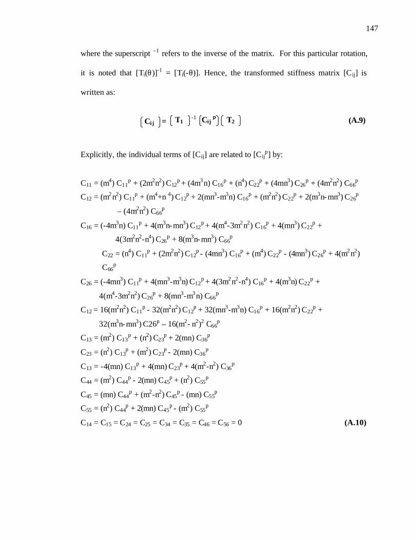
147
Cij p
= T2 T1 -1 Ci j
where the superscript –1 refers to the inverse of the matrix. For this particular rotation,
it is noted that [Ti(θ)]-1 = [Ti(-θ)]. Hence, the transformed stiffness matrix [C ij] is
written as:
(A.9)
Explicitly, the individual terms of [Cij] are related to [Cijp] by:
C11 = (m4) C11
p + (2m2n2) C12p + (4m3n) C16
p + (n4) C22p + (4mn3) C26
p + (4m2n2) C66p
C12 = (m2n2) C11p + (m4+n 4) C12
p + 2(mn3-m3n) C16p + (m2n2) C22
p + 2(m3n-mn3) C26p
– (4m2n2) C66p
C16 = (-4m3n) C11p + 4(m3n-mn3) C12
p + 4(m4-3m2n2) C16p + 4(mn3) C22
p +
4(3m2n2-n4) C26p + 8(m3n-mn3) C66
p
C22 = (n4) C11p + (2m2n2) C12
p - (4mn3) C16p + (m4) C22
p - (4mn3) C26p + 4(m2n2)
C66p
C26 = (-4mn3) C11p + 4(mn3-m3n) C12
p + 4(3m2n2-n4) C16p + 4(m3n) C22
p +
4(m4-3m2n2) C26p + 8(mn3-m3n) C66
p
C12 = 16(m2n2) C11p - 32(m2n2) C12
p + 32(mn3-m3n) C16p + 16(m2n2) C22
p +
32(m3n-mn3) C26p – 16(m2- n2)2 C66p
C13 = (m2) C13p + (n2) C23
p + 2(mn) C36p
C23 = (n2) C13p + (m2) C23
p - 2(mn) C36p
C13 = -4(mn) C13p + 4(mn) C23
p + 4(m2-n2) C36p
C44 = (m2) C44p - 2(mn) C45
p + (n2) C55p
C45 = (mn) C44p + (m2-n2) C45
p - (mn) C55p
C55 = (n2) C44p + 2(mn) C45
p - (m2) C55p
C14 = C15 = C24 = C25 = C34 = C35 = C46 = C56 = 0 (A.10)

148
APPENDIX C: SINGULAR STRESS SOLUTION
This appendix provides details in solving the singular stress solution in the local
analysis of the free edge stress field. This includes determining the strength of the edge
singularity, λ and the angular variations, σ?ij(θ) of the local stress field. The formulation
begins assuming that an edge singularity exists at the interface between two adjacent
plies. The upper ply is denoted as α and the lower ply as β . The stress and
displacement equations for each ply are given in Eq. (2.19) and (2.20), respectively.
Assuming the plies are perfectly bonded, the displacement components (u, v and w)
and the interlaminar stress components (σz , τxz and τyz ) are continuous across the
interface. All other surfaces of the plies are traction free. From Eq. (2.19) and (2.20),
the local boundary conditions yield a system of twelve homogenous equations is
obtained. These are given as:
For the stress- free boundary conditions of the upper α ply:
1. σy α= 0 : Σ Ak
α µk2 Γk(θ=π /2) = 0
2. τxyα= 0 : Σ Ak
α µk ηkΓk(θ=π /2) = 0 (B.1)
3. τyzα= 0 : Σ Ak
α µk Γk(θ=π /2) = 0
For the stress- free boundary conditions of the β ply:
4. σy β= 0 : Σ Ak
β µk2 Γk(θ=−π /2) = 0
5. τxyβ= 0 : Σ Ak
βµk ηkΓk(θ=−π /2) = 0 (B.2)
6. τyzβ= 0 : Σ Ak
β µk Γk(θ=−π /2) = 0
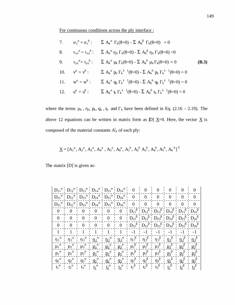
149
For continuous conditions across the ply interface :
7. σzα = σz
β : Σ Akα Γk(θ=0) - Σ Ak
β Γk(θ=0) = 0
8. τxzα = τxz
β : Σ Akα ηk Γk(θ=0) - Σ Ak
β ηk Γk(θ=0) =0
9. τyzα= τyz
β : Σ Akα µk
Γk(θ=0) - Σ Akβ µk
Γk(θ=0) = 0 (B.3)
10. vα = vβ : Σ Akα pk Γk
λ +1(θ=0) - Σ Akβ pk Γk
λ +1(θ=0) = 0
11. wα = wβ : Σ Akα qk Γk
λ +1(θ=0) - Σ Akβ qk Γk
λ +1(θ=0) = 0
12. uα = uβ : Σ Akα tk Γk
λ +1(θ=0) - Σ Akβ tk Γk
λ +1(θ=0) = 0
where the terms µk , ηk, pk, qk , tk and Γk have been defined in Eq. (2.16 - 2.19). The
above 12 equations can be written in matrix form as [D] X=0. Here, the vector X is
composed of the material constants Aik of each ply:
X = [A1α, A2
α, A3α, A4
α , A5α, A6
α, A1β, A2
β A3β, A4
β, A5β, A6
β] T
The matrix [D] is given as:
D11
α D12α D13
α D14α D15
α D16α 0 0 0 0 0 0
D21α D22
α D23α D24
α D25α D26
α 0 0 0 0 0 0
D31α D32
α D33α D34
α D35α D36
α 0 0 0 0 0 0 0 0 0 0 0 0 D11
β D12β D13
β D14β D15
β D16β
0 0 0 0 0 0 D21β D22
β D23β D24
β D25β D26
β
0 0 0 0 0 0 D31β D32
β D33β D34
β D35β D36
β 1 1 1 1 1 1 -1 -1 -1 -1 -1 -1
η1α η2
α η3α η1
α η2α η3
α η1β η2
β η3β η1
β η2β η3
β µ1
α µ2α µ3
α µ1α µ2
α µ3α µ1
β µ2β µ3
β µ1β µ2
β µ3β
p1α p2
α p3α p1
α p2α p3
α p1β p2
β p3β p1
β p2β p3
β
q1α q2
α q3α q1
α q2α q3
α q1β q2
β q3β q1
β q2β q3
β t1α t2α t3α t1α t2α t3α t1β t2β t3β t1β t2β t3β

150
where
D11α = (µ1
α)2 (µ1α)λ
D12α = (µ2
α)2 (µ2α)λ
D13α = (µ3
α)2 (µ3α)λ
D14α = (µ1
α)2 (µ1α)λ
D15α = (µ2
α)2 (µ2α)λ
D16α = (µ3
α)2 (µ3α)λ
D21α = η1
α(µ1α) (µ1
α)λ
D22α = η2
α(µ2α) (µ2
α)λ
D23α = η3
α(µ3α) (µ3
α)λ
D24α = η1
α(µ1α) (µ1
α)λ
D25α = η2
α(µ2α) (µ2
α)λ D26
α = η3α(µ3
α) (µ3α)λ
D31α = (µ1
α) (µ1α)λ
D32α = (µ2
α) (µ2α)λ
D33α = (µ3
α) (µ3α)λ
D34α = (µ1
α) (µ1α)λ
D35α = (µ2
α) (µ2α)λ
D36α = (µ3
α) (µ3α)λ
D11
β = (µ1α)2 (µ1
α)λ
D12β = (µ2
α)2 (µ2α)λ
D13β = (µ3
β)2 (µ3β)λ
D14β = (µ1
β)2 (µ1β)λ
D15β = (µ2
β)2 (µ2β)λ
D16β = (µ3
β)2 (µ3β)λ
D21β = η1
β(µ1β) (µ1
β)λ
D22β = η2
β(µ2β) (µ2
β)λ
D23β = η3
β(µ3β) (µ3
β)λ
D24β = η1
β(µ1β) (µ1
β)λ
D25β = η2
β(µ2β) (µ2
β)λ D26
β = η3β(µ3
β) (µ3β)λ
D31β = (µ1
β) (µ1β)λ
D32β = (µ2
β) (µ2β)λ
D33β = (µ3
β) (µ3β)λ
D34β = (µ1
β) (µ1β)λ
D35β = (µ2
β) (µ2β)λ
D36β = (µ3
β) (µ3β)λ

151
This is an eigenvalue problem in which the strength of the singularity, λ is the
eigenvalue and the X is the eigenvector. λ can be computed when the determinant of
[D] vanishes. This process has been executed by the MAPLE (version 7) software
package to handle the trigonometric, algebraic calculations and the plotting features
needed. Below is a sample MAPLE command file to demonstrate the steps used in this
analysis. Comments are added to the command file to assist the user in understanding
and executing the program.
Command file:
** Denotes a comment and is not a maple command (remove when executing).
Commands ending with a colon (:) denote that the maple output is suppressed,
while a semicolon denote output is displayed on screen.
** Loads linear algebra package
with (linalg)
** Defines the compliance matrix [AJij] for the upper ply, α. Here, the actual values
are left blank. Note that we take advantage that certain quantities are zero and the
symmetry of the compliance matrix.
a11:= : (Type in compliance material constants for upper ply) a12:= : a13:= :
a15:= : a22:= : a23:= : a25:= : a33:= : a35:= : a44:= :

152
a55:= : a66:= : a14=a15=a24=a26=a34=a36=a36=a45=a46=a56=0:
a21:=a12:a31:=a13:a41:=a14:a51:=a15:a61:=a16:a32:=a23:a42:=a24:a52:=a25: a62:=a26:a43:=a34:a53:=a35:a63:=a36:a54:=a45:a64:=a46:a65:=a56: AJ:=matrix(6,6,[a11,a12,a13,a14,a15,a16,a21,a22,a23,a24,a25,a26,a31,a32,a33,a34,a35,a36,a41,a42,a43,a44,a45,a46,a51,a52,a53,a54,a55,a56,a61,a62,a63,a64,a65,a66]);
** [AJij] is reduced from a 6x 6 matrix to a 5x5 matrix [SJij] due the generalized plain
strain conditions. Using the relation given in Eq (2.16)
S11:=a11-a13*a13/a33:S12:=a12-a13*a23/a33:S16:=a16-a13*a63/a33: S22:=a22-a23*a23/a33:S24:=a24-a23*a43/a33:S26:=a26-a23*a63/a33: S44:=a44-a34*a34/a33:S45:=a45-a43*a53/a33:S55:=a55-a35*a35/a33: S66:=a66-a36*a36/a33: S14:=a14-a13*a43/a33: S15:=a15-a13*a53/a33: S25:=a25-a23*a53/a33: S46:=a46-a43*a63/a33:S56:=a56-a53*a63/a33: S21:=S12:S41:=S14:S51:=S15:S61:=S16:S42:=S24:S52:=S25: S62:=S26:S54:=S45:S64:=S46:S65:=S56: SJ:=matrix(5,5,[S11,S12,S14,S15,S16,S21,S22,S24,S25,S26,S41,S42,S44,S45,S46,S51,S52,S54,S55,S56,S61,S62,S64,S65,S66]);
** The six roots of the characteristic equation (u1i) in Eq (2.18) and Eq (2.19) are
solved
Biharm1:= ((S11*u1^4-2*S16*u1^3+(2*S12+S66)*u1^2-2*S26*u1 +S22))*((S55*u1^2-2*S45*u1+S44))-((S15*u1^3-(S14+S56)*u1^2 +(S25+S46)*u1-S24))^2=0;
solve(Biharm1,u1);
** The same procedure is used define the material properties [BJij] and solve its roots
(u2i) of the lower ply β .

153
b11:= : (Type in compliance material constants for lower ply) b12:= : b13:= :
b15:= : b22:= : b23:= : b25:= : b33:= : b35:= : b44:= : b55:= : b66:= : b14=b15=b24=b26=b34=b36=b36=b45=b46=b56=0: b21:=b12:b31:=b13:b41:=b14:b51:=b15:b61:=b16:b32:=b23:b42:=b24: b52:=b25:b62:=b26:b43:=b34:b53:=b35:b63:=b36:b54:=b45:b64:=b46:b65:=b56: BJ:=matrix(6,6,[b11,b12,b13,b14,b15,b16,b21,b22,b23,b24,b25,b26,b31,b32,b33,b34,b35,b36,b41,b42,b43,b44,b45,b46,b51,b52,b53,b54,b55,b56,b61,b62,b63,b64,b65,b66]);
K11:=b11-b13*b13/b33:K12:=b12-b13*b23/b33:K16:=b16-b36*b13/b33: K22:=b22-b23*b23/b33:K24:=b24-b23*b34/b33:K26:=b26-b23*b36/b33: K44:=b44-b34*b34/b33:K45:=b45-b34*b35/b33:K55:=b55-b35*b35/b33: K66:=b66-b36*b36/b33: K14:=b14-b34*b13/b33: K15:=b15-b35*b13/b33: K25:=b25-b23*b35/b33: K46:=b46-b34*b36/b33: K56:=b56-b35*b36/b33: K21:=K12:K41:=K14:K51:=K15:K61:=K16:K42:=K24:K52:=K25: K62:=K26:K54:=K45:K64:=K46:K65:=K56: SJ:=matrix(5,5,[K11,K12,K14,K15,K16,K21,K22,K24,K25,K26,K41,K42,K44,K45,K46,K51,K52,K54,K55,K56,K61,K62,K64,K65,K66]);
Biharm2:= (K11*u2^4-2*K16*u2^3+(2*K12+K66)*u2^2-2*K26*u2 +K22) *(K55*u2^2-2*K45*u2+K44)-(K15*u2^3-(K14+K56)*u2^2+(K25+K46)*u2-K24)^2=0; solve(Biharm2,u2);
** The material constants nk, pk, qk, and tk (k= 1..6)are calculated from Eq. (2.18),
(2.19), and (2.20). To define each constant, we use an alphabetic letter followed by two
numerical indices. The alphabetic letter refers to the material constant of the same
letter, while the first numerical index refers the ply considered (1 for the α ply, and 2
for the β ply) and the second numerical index refers to the kth solution of that variable.

154
This notation is used throughout the rest of the command file. Also, we note that
k=4,5,6 are the complex conjugates of the k=1,2,3 solutions for the corresponding
variable.
** For the α ply, u1i is first explicitly defined from the previous maple output, and then
corresponding constants nk, pk, qk, and tk are computed.
u11:= ; (Fill in uij for the upper ply, computed earlier) u12:= ; u13:= ; u14:=conjugate(u11);u15:=conjugate(u12);u16:=conjugate(u13);
n11:=-(S15*u11^3-(S14+S56)*u11^2+(S25+S46)*u11-S24)/(S55*u11^2-2*S45*u11+S44); n12:=-(S15*u12^3-(S14+S56)*u12^2+(S25+S46)*u12-S24)/(S55*u12^2-2*S45*u12+S44); n13:=-(S15*u13^3-(S14+S56)*u13^2+(S25+S46)*u13-S24)/(S55*u13^2-2*S45*u13+S44); n14:=conjugate(n11);n15:=conjugate(n12);n16:=conjugate(n13);
p11:=S11*u11^2 +S12-S14*n11+S15*n11*u11-S16*u11; p12:=S11*u12^2 +S12-S14*n12+S15*n12*u12-S16*u12; p13:=S11*u13^2 +S12-S14*n13+S15*n13*u13-S16*u13; p14:=conjugate(p11);p15:=conjugate(p12);p16:=conjugate(p13); q11:=S12*u11 +S22/u11 -S24*n11/u11 +S25*n11-S26; q12:=S12*u12 +S22/u12 -S24*n12/u12 +S25*n12-S26; q13:=S12*u13 +S22/u13 -S24*n13/u13 +S25*n13-S26; q14:=conjugate(q11);q15:=conjugate(q12);q16:=conjugate(q13);
t11:=S14*u11 +S24/u11 -S44*n11/u11 +S45*n11 -S46;
t12:=S14*u12 +S24/u12 -S44*n12/u12 +S45*n12 -S46;
t13:=S14*u13 +S24/u13 -S44*n13/u13 +S45*n13 -S46;
t14:=conjugate(t11);t15:=conjugate(t12);t16:=conjugate(t13);

155
** For the β ply, u2i is first explicitly defined from the previous maple output, and then
the corresponding constants nk, pk, qk, and tk are computed.
u21:= ; (Fill in uij for the lower ply, computed earlier) u22:= ; u23:= ; u24:=conjugate(u21);u25:=conjugate(u22);u26:=conjugate(u23);
n21:=-(K15*u21^3-(K14+K56)*u21^2+(K25+K46)*u21-K24)/(K55*u21^2-2*K45*u21+K44); n22:=-(K15*u22^3-(K14+K56)*u22^2+(K25+K46)*u22-K24)/(K55*u22^2-2*K45*u22+K44); n23:=-(K15*u23^3-(K14+K56)*u23^2+(K25+K46)*u23-K24)/(K55*u23^2-2*K45*u23+K44); n24:=conjugate(n21);n25:=conjugate(n22);n26:=conjugate(n23);
> p21:=K11*u21^2 +K12-K14*n21+K15*n21*u21-K16*u21; p22:=K11*u22^2 +K12-K14*n22+K15*n22*u22-K16*u22; p23:=K11*u23^2 +K12-K14*n23+K15*n23*u23-K16*u23; p24:=conjugate(p21);p25:=conjugate(p22);p26:=conjugate(p23); q21:=K12*u21 +K22/u21 -K24*n21/u21 +K25*n21-K26; q22:=K12*u22 +K22/u22 -K24*n22/u22 +K25*n22-K26; q23:=K12*u23 +K22/u23 -K24*n23/u23 +K25*n23-K26; q24:=conjugate(q21);q25:=conjugate(q22);q26:=conjugate(q23);
t21:=K14*u21 +K24/u21 -K44*n21/u21 +K45*n21 -K46; t22:=K14*u22 +K24/u22 -K44*n22/u22 +K45*n22 -K46; t23:=K14*u23 +K24/u23 -K44*n23/u23 +K45*n23 -K46; t24:=conjugate(t21);t25:=conjugate(t22);t26:=conjugate(t23);
** With the above constants and the appropriate boundary conditions, the 12x12 [D]
matrix in Eq. (2.23) is defined , where the variable ‘lambda’ represents the strength of
the singularity (λ).
D:=linalg[matrix](12,12,[ u11^2*(u11)^(lambda),u12^2*(u12)^(lambda),u13^2*(u13)^(lambda),u14^2*(u14)^(lambda),u15^2*(u15)^(lambda),u16^2*(u16)^(lambda),0,0,0,0,0,0, (u11)^(lambda)*n11*u11,(u12)^(lambda)*n12*u12,(u13)^(lambda)*u13*n13,n

156
14*u14*(u14)^(lambda),n15*u15*(u15)^(lambda),n16*u16*(u16)^(lambda),0,0,0,0,0,0, (u11)^(lambda)*u11,(u12)^(lambda)*u12,(u13)^(lambda)*u13,u14*(u14)^(lambda),u15*(u15)^(lambda),u16*(u16)^(lambda),0,0,0,0,0,0, 0,0,0,0,0,0,u21^2*(-u21)^(lambda),u22^2*(-u22)^(lambda),u23^2*(-u23)^(lambda),u24^2*(-u24)^(lambda),u25^2*(-u25)^(lambda),u26^2*(-u26)^(lambda), 0,0,0,0,0,0,n21*u21*(-u21)^(lambda),n22*u22*(-u22)^(lambda),n23*u23*(-u23)^(lambda),n24*u24*(-u24)^(lambda),n25*u25*(-u25)^(lambda),n26*u26*(-u26)^(lambda), 0,0,0,0,0,0,u21*(-u21)^(lambda),u22*(-u22)^(lambda),u23*(-u23)^(lambda),u24*(-u24)^(lambda),u25*(-u25)^(lambda),u26*(-u26)^(lambda), 1,1,1,1,1,1,-1,-1,-1,-1,-1,-1, n11,n12,n13,n14,n15,n16,-n21,-n22,-n23,-n24,-n25,-n26, u11,u12,u13,u14,u15,u16,-u21,-u22,-u23,-u24,-u25,-u26, p11,p12,p13,p14,p15,p16,-p21,-p22,-p23,-p24,-p25,-p26, q11,q12,q13,q14,q15,q16,-q21,-q22,-q23,-q24,-q25,-q26, t11,t12,t13,t14,t15,t16,-t21,-t22,-t23,-t24,-t25,-t26]); ** The characteristic equation of [D] is found by its determinant
chareq:=det(D): ** In order to solve for lambda, we need to find for the roots of the characteristic
equation of [D]. We do this by an iteration process. The characteristic equation is
plotted against a range of lambda values and the zeros are searched. The restrictions of
lambda are that it is real and must be between –1 and 0 due to energy constraints.
Char:=Re(chareq): plot(Char,lambda=-1..0); ** We note that one lambda value that satisfies the energy constraints. Lambda is
explicitly inputted from the above Maple output.
lambda:= ; ** Since [D] is rank deficient, the associated 1 x12 eigenvector X cannot be computed
unless one the constants of X is arbitrarily defined. In this case, we set X11 to unity.

157
Subsequently, the rest of the constants are found by solving the system of equations in
Eq. (2.23).
X11:=1; Sys:=({ (u11)^(lambda)*n11*u11*X11 + (u12)^(lambda)*n12*u12*X12 +(u13)^(lambda)*u13*n13*X13+ n14*u14*(u14)^(lambda)*X14 + n15*u15*(u15)^(lambda)*X15 + X16*n16*u16*(u16)^(lambda)=0, (u11)^(lambda)*u11*X11 + (u12)^(lambda)*u12*X12 + (u13)^(lambda)*u13*X13 + u14*(u14)^(lambda)*X14 + u15*(u15)^(lambda)*X15 + u16*(u16)^(lambda)*X16=0, u21^2*(-u21)^(lambda)*X21 + u22^2*(-u22)^(lambda)*X22 + u23^2*(-u23)^(lambda)*X23 + u24^2*(-u24)^(lambda)*X24 + u25^2*(-u25)^(lambda)*X25 + u26^2*(-u26)^(lambda)*X26=0, n21*u21*(-u21)^(lambda)*X21 + n22*u22*(-u22)^(lambda)*X22 + n23*u23*(-u23)^(lambda)*X23+ n24*u24*(-u24)^(lambda)*X24 + n25*u25*(-u25)^(lambda)*X25 + n26*u26*(-u26)^(lambda)*X26=0, u21*(-u21)^(lambda)*X21 + u22*(-u22)^(lambda)*X22 + u23*(-u23)^(lambda)*X23+ u24*(-u24)^(lambda)*X24 + u25*(-u25)^(lambda)*X25 + u26*(-u26)^(lambda)*X26=0, X11+X12+X13+X14+X15+X16-X21-X22-X23-X24-X25-X26=0, n11*X11+n12*X12+n13*X13+n14*X14+n15*X15+n16*X16-n21*X21-n22*X22-n23*X23-n24*X24-n25*X25-n26*X26=0, u11*X11+u12*X12+u13*X13+u14*X14+u15*X15+u16*X16-u21*X21-u22*X22-u23*X23-u24*X24-u25*X25-u26*X26=0, p11*X11+p12*X12+p13*X13+p14*X14+p15*X15+p16*X16-p21*X21-p22*X22-p23*X23-p24*X24-p25*X25-p26*X26=0, q11*X11+q12*X12+q13*X13+q14*X14+q15*X15+q16*X16-q21*X21-q22*X22-q23*X23-q24*X24-q25*X25-q26*X26=0, t11*X11+t12*X12+t13*X13+t14*X14+t15*X15+t16*X16-t21*X21-t22*X22-t23*X23-t24*X24-t25*X25-t26*X26=0}); fsolve(Sys,{X12,X13,X14,X15,X16,X21,X22,X23,X24,X25,X26}); ** End Program.

158
∆W = 1 2
σ ∆u da a+∆a
a
G = lim 1 2∆a
σij ∆ui da ∆a à 0
a+∆a
a
APPENDIX D: CRACK CLOSURE SCHEME
This appendix provides the details of the crack closure scheme for determining
the energy release rate. The scheme is designed for long, symmetrically stacked
laminates subjected under uni-axial strain, ex.. Assuming that edge delamination is the
only failure mode occurring during loading, the edge crack can be modeled as a line
crack propagating into the center of the laminate.
The crack closure scheme proposes that the elastic strain energy released during
a small incremental crack is equal to the work done in closing the crack to its original
length [57]. Let ao be the size of the delamination crack at a given interface. Under
critical loading, the crack will propagate an incremental amount, denoted as ∆a. Then,
the work needed (per unit thickness) to close the incremental crack is:
(C.1)
where σij (i,j = 1,2,3)is the stress distribution along ∆a of the closed surface, and ∆ui (I
= 1,2,3) is the relative displacements between the between the open surfaces along ∆a.
Substituting the individual stress components σij and the relative displacements
∆ui into above equation, the available energy release rate G can be written as:
(C.2)
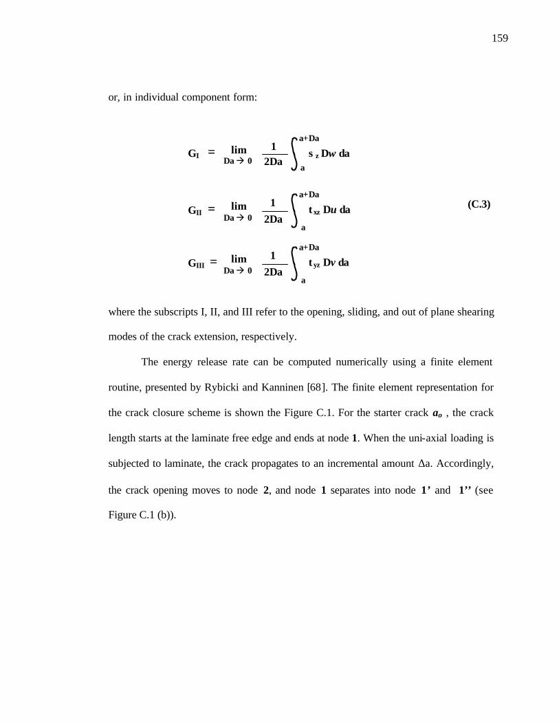
159
or, in individual component form:
(C.3)
where the subscripts I, II, and III refer to the opening, sliding, and out of plane shearing
modes of the crack extension, respectively.
The energy release rate can be computed numerically using a finite element
routine, presented by Rybicki and Kanninen [68]. The finite element representation for
the crack closure scheme is shown the Figure C.1. For the starter crack ao , the crack
length starts at the laminate free edge and ends at node 1. When the uni-axial loading is
subjected to laminate, the crack propagates to an incremental amount ∆a. Accordingly,
the crack opening moves to node 2, and node 1 separates into node 1’ and 1’’ (see
Figure C.1 (b)).
GII = lim 1 2∆a
τxz ∆u da ∆a à 0
a+∆a
a
GIII = lim 1 2∆a
τyz ∆v da ∆a à 0
a+∆a
a
GI = lim 1 2∆a
σz ∆w da ∆a à 0
a+∆a
a

160
Figure C.1. Finite element represent of the crack closure scheme
The stress and displacement fields in the laminate are approximated by nodal
forces and nodal displacements. Let ∆ei , i= 1,2, and 3 denote the displacement
components for the crack tip opening between nodes 1’ and 1’’ for the applied strain ex.
In addition, thermal loading is also applied to the laminate; this component becomes
important during the laminate curing process. Let ∆Ti be the displacement components
y
z
x
1
free edge
2
a + ∆a
∆ui
1’
1’’
node
y
z
x
1
free edge
2
a + ∆a
∆ui
1’
1’’
node
(b). Crack growth to size a + ∆a
y
z
x
1
a
free edge
2
∆a
node
(a). Starter crack of size a at the laminate free edge
y
z
x
1
a
free edge
2
∆a
node
y
z
x
1
a
free edge
2
∆a
node
(a). Starter crack of size a at the laminate free edge

161
G (ex, ∆T, a) = [ Ce ex + CT ∆T ]2 2t*
caused by this loading. Therefore, the total displacement, ∆ui, between these pair of
nodes can be expressed as:
∆ui = (∆ei) ex + (∆Ti) ∆T (for i = 1, 2 , 3) (C.4)
Let Fi represent the nodal forces needed to close the nodal gap from nodes1’ and 1’’
such that the associated displacements will recover their original position at node 1.
Fi = (Fe i) ex + (FTi) ∆T (for i = 1, 2 , 3) (C.5)
where Fe i and FTi are the coefficients for F due to a unit of ex and ∆T, respectively.
Accordingly, the work, ∆W, done during the incremental crack closure is given by:
∆W = ½ Fi ( ∆ui) (for i = 1, 2 , 3) (C.6)
Substituting Eq. (C.6) into Eq. (C.2), the energy release rate, G, for the given
crack size a can be approximated as:
G (ex, ∆T, a) = (∆W/∆a) = [(Fe i) ex + (FTi) ∆T] /2∆a (C.7)
Combining Eq. (C.4), Eq. (C.5), into Eq. Eq. (C.7), G may be written explicitly in
terms of ex and ∆T:
(C.8)
where the coefficients Ce and CT are

162
Ce = [ (Fe i) (∆ei)] / (2∆a)
CT = [ (Fe i) (∆Ti)] / (2∆a) (C.9)
and the parameter t* is a dimensionless scaling factor between the finite element model
and the physical laminate. Here, coefficients Ce and CT are associated the individual
loadings ex and ∆T, respectively; however, they are independent of the actual loading
values. The units for the Ce is energy per unit area, CT is energy per unit area per ∆T2,
and CeT is energy per unit area per ∆T.
In Eq. (C.8), the energy release rate G from includes all the crack extension
modes (I, II, III). However, G can also be separated into component form, given as:
GI = [F3 (∆u3)]/2∆a
GII = [F2 (∆u2)]/2∆a (C.10)
GIII = [F1 (∆u1)]/2∆a

163
VITA
Simon Chung was born on September 16,1974 in Philadelphia, Pennsylvania.
He received both his B.S. in Mechanical Engineering (1997) and M.S. in Mechanical
Engineering (1999) from Drexel University.
As an undergraduate student he had co-operative work experience at the City of
Philadelphia as a city surveyor, and at E.I. Dupont de Nemours as research assistant for
the Automotive Finishes group at the Experimental Station in Wilmington, Delaware.
As a graduate student, Simon’s primary research was the analytical and numerical
analyses of the fracture behavior of composite materials under the tutelage of Dr.
Albert Wang. He also worked as teaching assistant for Statics, Dynamics, Mechanics
of Materials, Experimental Mechanics Laboratory, Materials II and Advanced
Engineering Math under numerous professors. He received an award for Teaching
Assistant Excellence in April 2001.
Upon graduation, Simon hopes continue his research in the structural and
fracture mechanics field, while seeing the world. He also hopes to return as a teacher
and an educator.

164