Embed Size (px)
Citation preview

EFFECTS OF HOT STREAK AND
PHANTOM COOLING ON HEAT
TRANSFER IN A COOLED
TURBINE STAGE INCLUDING
PARTICULATE DEPOSITION
THE OHIO STATE UNIVERSITYBrian Casaday, Derek Lageman
Ali Ameri, Jeffrey Bons
2011 UTSR Workshop – 26 Oct. 2011
1

MOTIVATION
2
• Future gas turbines operating with HHC fuels will have higher turbine inlet
temperatures relative to natural gas operation.
• Increased temperatures require better materials and more efficient cooling
schemes. Increased cooling is unacceptable, so coolant must be used smarter
and more sparingly.
• Requires better prediction of combustor exit temperature distribution (pattern
factor) and migration of high temperature core (hot streak) through high
pressure turbine.
Prediction of hot streak migration in uncooled turbine stage using
inviscid, unsteady simulation. (Shang & Epstein, JTurbo 1997)
Time averaged surface temperature on rotor
suction (left) and pressure (right) surfaces.
Hot Streak enters center
of vane passage
Pile-up
on Rotor
PS
Migration to
rotor blade
root.

MOTIVATION
3
•HHC fuels may contain airborne ash particulate that then
deposits in the turbine – degrading performance. Hot streaks
will result in preferential deposition. Predictive tools for
modeling the combined effect of hot streaks and deposition are
necessary for risk assessment and mitigation.
First stage nozzle volcanic
ash deposition from RB211
following Mt Gallungung
eruption, 24 June 1982
(Chambers)
Elevated ash
deposition
aligned with fuel
nozzle locations -
evident every
other NGV

CRITICAL NEED
4
Additional research is NEEDED to…
• model hot streak migration in a modern, cooled first
stage turbine
• model effect of hot streak on coolant flow (phantom
cooling)
• model deposition in HHC, elevated temperature
environment
• validate models with steady (stator) and unsteady
(rotor) experimental data

OBJECTIVES
5
• The objective of this work is to develop a validated modeling capability
to characterize the effect of hot streaks on the heat load of a modern
gas turbine.
• As a secondary objective the model will also be able to predict
deposition locations and rates.
This will be accomplished for a cooled turbine stage (stator and rotor)
AND
will be validated with experimental data from facilities at OSU.
The effort includes both experimental and computational components,
with work divided into three phases of increasing complexity:
1) Uncooled Vane
2) Cooled Vane
3) Uncooled/Cooled Rotor

RESEARCH TEAM
6
Dr. Jeffrey BonsProfessorDepartment of Mechanical and Aerospace EngineeringOhio State UniversityColumbus, OH
Dr. Ali AmeriResearch ScientistDepartment of Mechanical and Aerospace EngineeringOhio State UniversityColumbus, OH
TEAM LEADFocus: Experimental Heat Transfer and Deposition Measurements in OSU Hot Cascade Facility
Co-PIFocus: Deposition Model Development and Heat Transfer CFD
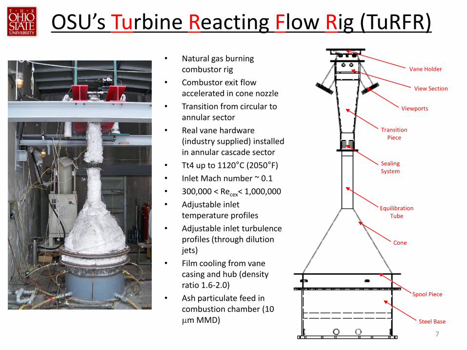
OSU’s Turbine Reacting Flow Rig (TuRFR)
• Natural gas burning combustor rig
• Combustor exit flow accelerated in cone nozzle
• Transition from circular to annular sector
• Real vane hardware (industry supplied) installed in annular cascade sector
• Tt4 up to 1120°C (2050°F)
• Inlet Mach number ~ 0.1
• 300,000 < Recex< 1,000,000
• Adjustable inlet temperature profiles
• Adjustable inlet turbulence profiles (through dilution jets)
• Film cooling from vane casing and hub (density ratio 1.6-2.0)
• Ash particulate feed in combustion chamber (10
m MMD)
7
Steel Base
Equilibration Tube
Cone
Spool Piece
View Section
Viewports
Transition Piece
Sealing System
Vane Holder

OSU’s Turbine Reacting Flow Facility (TuRFR)
8
Film Cooling Supply
Circular to Rectangular Transition
Top Section/
Vane container
Rectangular to Annular Transition
Vane Holder and Upstream Conditioning
Interchangeable Dilution Plates for Pattern Factors
Dilution Jet Supply

Typical TuRFR Test Sequence
9
t = 0 t = 2 min t = 8 min
t = 11 min Post testTime Lapse ImagesWyoming
Sub-Bituminous AshTest Conditions:
Tt4~1900FMin=0.90

Post Test Diagnostics - MetrologyPre Test Scan
Post Test Scan
Deposit height indicated in contour map
relative to Pre-Test Datum

11
PHASE 1: Uncooled Vane• Revisit OSU’s current deposition model
• Consult with industry to determine representative hot
streak for power turbine.
• Generate hot streak in TuRFR
• Measure hot streak migration and adiabatic wall
temperature (uncooled vane)
• Measure deposition patterns and rates with hot streaks
• Compare model predictions with TuRFR hot streak and
deposition measurements.
• Modify model as needed.

12
PHASE 2: Cooled Vane• Measure hot streak migration and wall
temperature for cooled vane
• Measure deposition patterns and rates with hot
streaks for cooled vane
• Compare model predictions with TuRFR hot
streak and deposition measurements.
• Modify model as needed.
• Propose and explore design modifications that
will mitigate particulate deposition on turbine
vanes.

13
PHASE 3: Rotor• Incorporate deposition model into unsteady rotor-stator
code
• Extract hot streak data from OSU GTL rotating uncooled
turbine test data
• Extract hot streak data from OSU GTL rotating cooled
turbine test data
• Geometry modeling and gridding
• Compare model predictions with rotating data.
• Modify model as needed.
• Propose and explore design modifications that will
mitigate particulate deposition on turbine rotors.

14
Accomplishments
• Fabricated dilution plates for hot streak generation
in TuRFR
• Preliminary CFD Study:
• model hot streak migration in E3 vane.
• model deposition with hot streak in E3 vane using
critical viscosity deposition model.
• Canvasing literature for improved deposition models
•Actively pursuing sources for unsteady hot streak
data

15
• Modeling Background
• Particle Trajectory
• Deposition Models
• Verification
• Hot Streak Modeling
• Model Specifications
• Modeling Results
• Further Work
• Data
Preliminary Hot Streak
CFD Study

16
BackgroundNumerical study of deposition growth on 3D
turbine vanes by:
• Accurate capturing of flow physics for 3D turbine
passage
• Utilizing models for predicting particle trajectories in
3D flow fields
• Utilizing existing deposition models while exploring
mechanisms for improved modeling
• Locating areas of high deposition and determining
causes of increased deposition
17
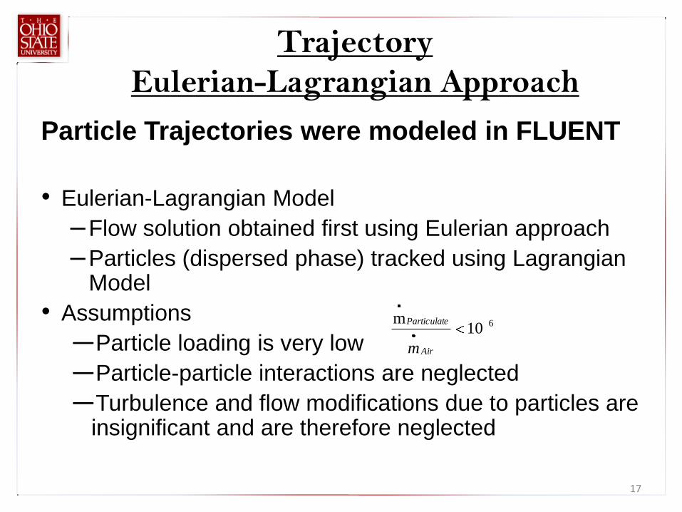
Particle Trajectories were modeled in FLUENT
• Eulerian-Lagrangian Model
–Flow solution obtained first using Eulerian approach
–Particles (dispersed phase) tracked using Lagrangian Model
• Assumptions
―Particle loading is very low
―Particle-particle interactions are neglected
―Turbulence and flow modifications due to particles are insignificant and are therefore neglected
Trajectory
Eulerian-Lagrangian Approach
610m
Air
eParticulat
m

18
Dispersed Phase
• Lagrangian approach solves the dispersed phase by
integrating the particle equation of motion.
• Forces considered: drag force modified with
Cunningham correction factor, Saffman Lift Force
• Forces not considered: Thermophoretic, Brownian,
Magnus, History effect, Gravitational, Buoyancy,
Intercollision

19
Trajectory
1 μm particles
(Stk = 0.01)
20 μm particles
(Stk = 4.0)
50 μm particles
(Stk = 25)

20
• We use two models for deposition
• Critical Velocity and Critical Viscosity
• The Crit. Vis. model, for many known compositions, may be used without the need for empirical fitting.
Deposition Models
1200 1250 1300 1350 1400 1450 1500 1550 16000
20
40
60
80
100
120
Temp (K)
Pro
ba
bili
ty o
f S
tickin
g u
po
n I
mp
act
(%)
• Viscosity-Temperature
relationship (Senior et al.) is
used.

21
Injection Properties
• Particles injected from
several locations
dispersed across inlet
• Assumes uniform
distribution of particulate
• Assumes particles are in
equilibrium with flow (i.e.
thermal and local
velocity)
Particle Injection
22
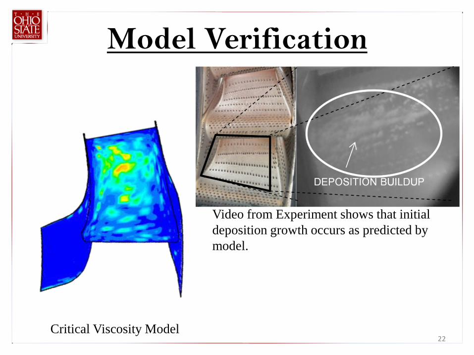
Model Verification
Critical Viscosity Model
Video from Experiment shows that initial
deposition growth occurs as predicted by
model.

23
Studying the effects hot streaks have on deposition
leads to better fidelity modeling
• Deposition has a strong dependence on temp.
thus H.S. in vane passages can lead to additional
deposition.
• They play an important role in the unsteady rotor
passage flow and heat transfer.
• HS can affect film cooling: both removing cooling
from where one hopes it would go AND
necessitating more cooling in regions where the
HS passes close to the surface
Why Hot Streaks?

24
Studied deposition growth on a 3D turbine vane with Hot
Streaks
• Hot streak profiles
• Axisymmetric profiles (w.r.t combustor axis)
• Gaussian temp. variation (peaking at center)
• Flat Turb. Profile of 5% (Gaussian future study )
• Hot streaks arranged (24 hr. Clock) with a two vane
pitch between the streaks.
• Use E3 Vane Model (Aero-Engine)
Hot Streak Model

25
Geometry and Grid
GE- E3 HP-Vane
Extended inlet
26
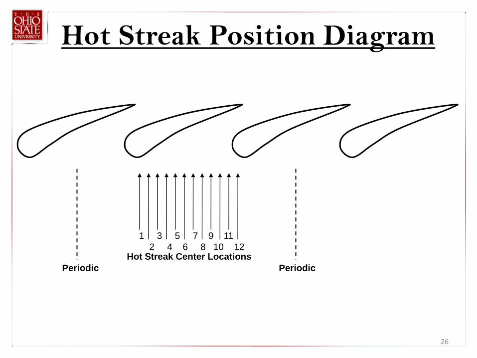
Hot Streak Position Diagram
Periodic
Hot Streak Center Locations
Periodic
1 3 5 7 9 11
2 4 6 8 10 12

27
Hot Streak Inlet Temperature Profiles
•One Streak per vane doublet.

28
Hot Streak Coherence
Contours of Total Temperature (K)
29
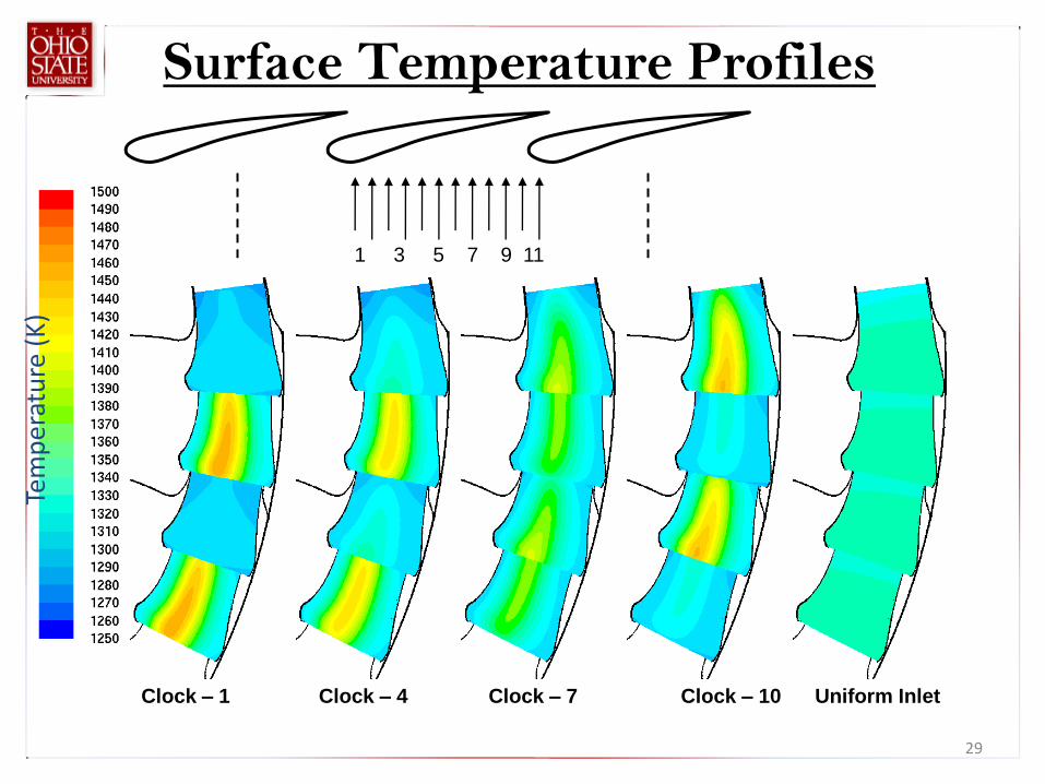
Surface Temperature Profiles
Clock – 1 Clock – 4 Clock – 7 Clock – 10 Uniform Inlet
Tem
per
atu
re (
K)
1 3 5 7 9 11

30
Deposition Modeling
• Used JBPS Ash composition.
Mass
Mean
Diamet
er
Bulk
Density
Element Weight %
Na Mg Al Si P S K Ca Ti V Fe Ni
13.4 µm
2.32
g/cc
6.9 3.6 18 47 1.6
1.
8
2.
6
8.7 1.6 0 6.4 0
CP (J/kg-
K)
K(W/m-
K)
984 0.5

31
Deposition Locations
Mass
Mean
Diamet
er
Bulk
Densit
y
Element Weight %
Na Mg Al Si P S K Ca Ti V Fe
N
i
13.4
µm
2.32
g/cc
6.9 3.6 18 47 1.6
1.
8
2.
6
8.
7
1.
6
0
6.
4
0
0.1
0
0.05
0.02
5
0.07
5
Clock – 1 Clock – 4 Clock – 7 Clock – 10 Uniform Inlet
1 3 5 7 9 11

32
-20 0 20 40 60 80 1000
200
400
600
800
1000
1200
1400
1600
1800
2000
Percent Chord
Hot Vane
Cold vane
Uniform Temp
0 10 20 30 40 50 60 70 80 90 1000
500
1000
1500
2000
2500
Percent Span
Hot Vane
Cold vane
Uniform Temp
Chord/Span Integrated Deposition
At 1 o’clock position
spanwise averaged
depositionchordwise averaged
deposition

33
1 2 3 4 5 6 7 8 9 10 11 12 13 14 15 16 17 18 19 20 21 22 23 240
5
10
15
20
25
30
35
40
45
Clocking Position
Captu
re E
ffic
iency (
%)
2 micron
4 micron
6 micron
8 micron
10 micron
Capture Efficiency Plot
Capture efficiency defined as total deposition on single vane divided by half of
particulate injected into vane doublet geometry
0.3 0.31 0.32 0.33 0.34 0.35 0.36 0.37 0.38 0.39-0.04
-0.03
-0.02
-0.01
0
0.01
0.02
0.03
0.04
34
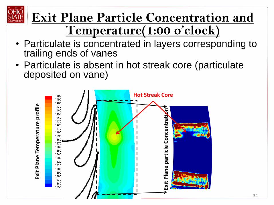
Exit Plane Particle Concentration and Temperature(1:00 o’clock)
• Particulate is concentrated in layers corresponding to trailing ends of vanes
• Particulate is absent in hot streak core (particulate deposited on vane)
Exit
Pla
ne
par
ticl
e C
on
cen
trat
ion
Exit
Pla
ne
Te
mp
era
ture
pro
file
Hot Streak Core

35
• For the turbulence level attempted, hot streaks
survive the vane passages.
• The relative position (and count ratio) of H.S. w.r.t. to
the vanes affect the deposition patterns.
• The relative position of H.S. w.r.t. to the vanes affect
particulate content of the flow downstream of the
vanes.
• The effect of H.S. on deposition is strongly related to
the Stokes number.
Conclusions of Preliminary
Study

36
It has been previously observed that:
• Hot gases from the streaks migrate to the pressure
side while cooler gases accumulate on the suction
side.
• Position of hot streaks with respect to the vane
impacts the migration path through the rotor passage
and heat transfer
• Buoyancy causes the hot gases to sink to the roots of
the blades
• Film cooling is made difficult by the action of H.S. not
following expected streamlines.
Effect of H.S. on Blades

37
• Hot Streaks modify wall heat transfer by both
modifying the flow field and imposing a higher thermal
potential on blades.
• Effect on heat transfer may not be described by the
adiabatic wall temperature distribution alone.
• Heat transfer coefficient, defined properly, can show
the effect of the hot streak on the blade heat transfer.
• We may be able to define h, heat transfer coefficient
that is flow dependent; h = qw / (Taw-Tw) for a given
form of hot streak.
Blade Heat Transfer
38
• Unsteady h may be computed by:
―Using an Isothermal Condition to get Qwall
―Using an adiabatic condition to get Taw
―using a phase locked condition
―h=Qwall/ (Taw-Tw) and then averaged.
• For uniform inlet, heat transfer can be computed in
the same manner.
• The effect of the hot streak can be discerned from the
difference.
Further Details

39
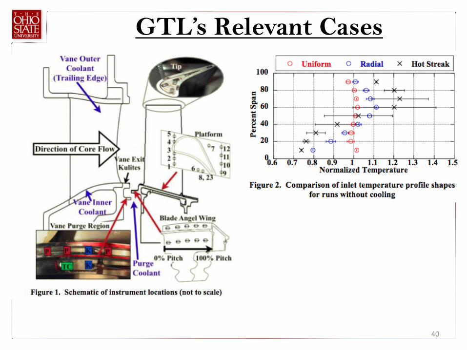
• Experiments on 1 ½ stage HP turbines were
conducted at OSU GTL
• Both uncooled vane and cooled vane.
• Hot Streak targeted at mid-pitch or vane leading
edge
• Hot Streak intensity varied
• Cooling rate varied
• Qwall measured
We will use the data sets pending access.
GTL’s Relevant Cases
40
GTL’s Relevant Cases

41
GTL’s Relevant Cases

42
Deposition Modeling
• Critical Viscosity Model
• probability of sticking exclusive function of
particle viscosity and thus f(Temp) ONLY.
• NO sensitivity to particle size, impact velocity or
angle of impingement
• Critical Velocity Model
• particle sticks IF normal velocity < critical
velocity
• critical velocity is f(size, Youngs Modulus,
Poissons ratio)
• Youngs Modulus is f(Temp)
• DOES NOT model plastic deformation!!!

43
Critical Viscosity Model
Motivated by the observed
trend that the Adhesion
Efficiency of small (53-74 m)
microspheres increases as
Temperature increases and
viscosity decreases!
Lower viscosity means that the particle is more likely
to “flow” (i.e. deform) upon impact with the surface.
This is PLASTIC deformation. As the particle
plastically deforms, the contact area with the surface
increases and thus the adhesion force (proportional to
contact area) increases.
SRINIVASACHAR, S. “An experimental study of the inertial deposition of ash under coal
combustion conditions.” Symposium (International) on Combustion, v. 23 issue 1, 1991, p.
1305-1312.

44
Critical Viscosity Model
Based on these
observations, Tafti and
Sreedharan (IGTI 2010)
concluded that once the
particle reaches some
critical viscosity, it will
ALWAYS stick to the
surface.
Below this critical viscosity (or Sticking
Temperature, Ts) the probability of
sticking (Ps) could be determined using
a ratio of the “critical” viscosity to the
particle viscosity at temperature.
Sreedharan, S.S., Tafti, D.K., 2010. Composition dependent model for the prediction of syngas ash deposition in
turbine gas hotpath. International Journal of Heat and Fluid Flow Volume 32, Issue 1, February 2011, Pages 201-211

45
Critical Viscosity Model
As such, the problem
reduces to finding Ts and (T)
For pure substances, (T) can be
found experimentally using a
viscometer and Ts can be found by
heating a cube of material until it
softens and deforms.
Ash particulate is composed of a variety of
inorganic compounds depending on the
type of ash that it being used. The strength
of the bonds that these compounds form
can be used to estimate viscosity, or how
easily it can PLASTICALLY deform.
(Empirically based on ratios of glass
formers to modifiers, Senior and
Srinivisachar [1995])

46
Critical Viscosity Model
Using the model of Senior
and Srinivasachar, Tafti and
Sreedharan estimated the Ts
and (T) distribution for their
ash and compared their
predicted capture efficiency
to the experiment of Wood
et al. (24 m PVC particles)
and found reasonable
agreement. Sreedharan, S.S., Tafti, D.K., 2010. COMPOSITION
DEPENDENT MODEL FOR THE PREDICTION OF
SYNGAS ASH DEPOSITION WITH APPLICATION TO A
LEADING EDGE TURBINE VANE. ASME Paper No.
GT2010-23655
Wood et al. (IGTI 2010) 24micron PVC particles
with Ts = 533K (Stokes=0.12)

47
Critique of the Critical Viscosity Model
•Viscosity influences the amount of plastic deformation
that occurs for a given impact condition – the greater the
plastic deformation, the higher the propensity for sticking!
•The energy required to plastically deform the particle
comes from the KINETIC ENERGY at impact.
•Kinetic energy is a function of velocity and size (mass) of
the particle.
Thus, the probability of sticking should also
depend on impact velocity and particle size.

48
Critique of the Critical Viscosity Model
Upon impact, the particle experiences BOTH elastic and
plastic deformation.
Amount of each deformation will no
doubt depend on structural
mechanics (E or ), which are both
functions of temperature.
Temperature
Elastic Deformation
Plastic
Deformation
But it will also depend on impact
kinetic energy (e.g. clay projectile)
Impact KE
Elastic Deformation
Plastic
Deformation

49
Critical VELOCITY Model
Motivated by the observed trend that the rebound of small
particles requires some minimum energy to overcome
adhesion force!
• Particle represented by mass, spring, and contact platform.
• Upon contact, spring compresses.
• Compressed spring releases energy propelling particle from wall
• Adhesion force on contact platform causes slight tension of spring
before RELEASE or CAPTURE.
• (Simplified model has constant contact area.)

50
Critical VELOCITY Model
Hertzian contact mechanics predict
increased contact surface area due to
ELASTIC deformation upon impact!
• Particle represented by elastic sphere
• Upon contact, sphere deforms.
• Energy stored in compression propels particle from wall
• Adhesion force on contact surface area causes slight tension of
particle before RELEASE or CAPTURE.
• Contact surface area varies with time.
51
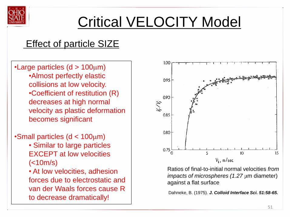
Critical VELOCITY Model
Effect of particle SIZE
•Large particles (d > 100 m)
•Almost perfectly elastic
collisions at low velocity.
•Coefficient of restitution (R)
decreases at high normal
velocity as plastic deformation
becomes significant
•Small particles (d < 100 m)
• Similar to large particles
EXCEPT at low velocities
(<10m/s)
• At low velocities, adhesion
forces due to electrostatic and
van der Waals forces cause R
to decrease dramatically!
Ratios of final-to-initial normal velocities from
impacts of microspheres (1.27 m diameter)
against a flat surface
Dahneke, B. (1975). J. Colloid Interface Sci. 51:58-65.

52
Critical VELOCITY ModelBrach and Dunn (ND, 1992)
developed a model to estimate
the work required to overcome
the adhesion force (WA). The
model is based on particle
kinematics and ONLY accounts
for elastic deformation.
WA is a function of:• particle properties (k1 is function of
Youngs Modulus and Poisson Ratio)
• surface properties (k2 is function of
Youngs Modulus and Poisson Ratio)
• size (r is sphere radius)
• surface energy adhesion parameter ( )
• normal impact velocity (vn)
• coefficient of Restitution (R)
• mass (m)
• normal release velocity (Vn)
2 equations, 3 unknowns
Requires empirical
estimate for R
- Fit coefficients k and p
- Example: for NH4Fl
spheres, k=45.3 and
p=0.718

53
Critical VELOCITY ModelBrach and Dunn (UND, 1992) compared kinematic impact model
with experimental data and developed empirical fits.
Primarily interested in determining coefficient of Restitution and effect of ELASTIC deformation.

54
Critical VELOCITY Model
• For the case of R=0 (i.e. deposition),
Brach and Dunn (UND, 1992) developed
an expression for the critical NORMAL
velocity below which particle capture
was certain.
• Critical velocity is a function of particle
and surface properties, particle size,
mass and R.
• El-Batsh and Haselbacher (2000,2002)
used this model to predict deposition in a
turbine vane. Compared to experimental
data of Parker and Lee (1972) – uranine
particles with double-stick tape on vane.

55
Critical VELOCITY Model• El-Batsh and Haselbacher accounted for the variation in particle
properties (E) with temperature using empirical fits to data.

56
Critical VELOCITY Model• Ai et al. (2008) used Brach and Dunn as well as El-Batsh and
Haselbacher models to compare experimental capture efficiency (ash
deposition) with predictions.
• 2D CFD model• The E obtained in this model by fitting
experimental data (T= 1293 K to 1453K) • Dependence of Young’s Modulus on temperature

57
Critique of Critical VELOCITY Model
• Model includes particle kinematics, KE of
impact, adhesion force, elastic deformation
• Model does NOT include PLASTIC
deformation!

58
Combination of the Models
• Critical Viscosity is dependent upon the
effect of plastic deformation occurring at
high temperatures
•Critical Velocity is dependent upon the
effect of the adhesion force occurring at
lower velocities
•An impact model that incorporates both
adhesion and plastic deformation would be
optimal

59
Combination of the Models
•The model needs to be dependent on all the outputs
of CFD and known properties of the particle and the
substrate
•CFD outputs• Particle temperature
• Particle size
• Particle mass
• Particle velocity
• Particle impingement angle
•Properties• Surface irregularities (roughness)
•Modulus of Elasticity
•Poisson’s Ratio
•Yield Stress

Current Elastic-Plastic Impact Models• Cold Spraying
– Metal on metal impact at supersonic speeds
• Molecular Bonding
– Attraction between the molecules of a particle
• FEM
– Meshing particles and surfaces to simulate the impact
• Energy Methods
– Using Energy Analysis to find final Kinetic energy
• Yield Stress determination
– Stress over the yield, plastically deforms the particle
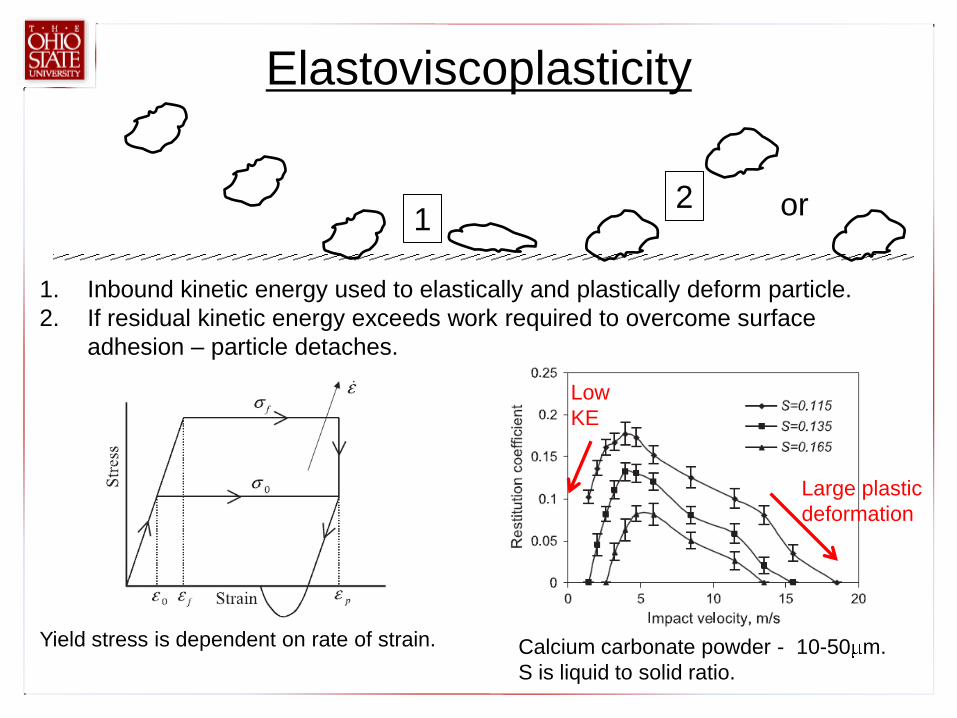
Elastoviscoplasticity
or
1. Inbound kinetic energy used to elastically and plastically deform particle.
2. If residual kinetic energy exceeds work required to overcome surface
adhesion – particle detaches.
12
Yield stress is dependent on rate of strain. Calcium carbonate powder - 10-50 m.
S is liquid to solid ratio.
Large plastic
deformation
Low
KE
Elastoviscoplasticity• Technique is sensitive to the parameters desired for the
deposition model
– Temperature
– Size
– Mass
– Velocity
– Properties of the particle and surface
• Some variations include adhesion
• Calculations can easily be made for each impacting particle
– Requires the data for yield stress
– This data can be acquired through experimentation or empirical modeling

Model Validation
• Optical test section mounted to
TuRFR exit.
• Canted flat plate target.
• Particle shadow velocimetry used to
measure: velocity, impact angle,
sticking probability, size, acceleration

64
Gantt Chart
Year 1 Year 2 Year 3
Phase 1
-Model Dvlpmnt
-Industry HS
input
-Uncooled vane
simulations
-TuRFR testing
Phase 2
-Cooled vane
simulations
-Experimental
validation
Phase 3
-Rotor
simulations
-Experimental
validation

QUESTIONS?

• Adjustment to rigid body model– Explicit parameter to represent the effect of adhesion– Kinetic instead of kinematic coefficient of rolling
resistance– Modification to parameters to account for oblique
impacts as well as normal impacts– Modification to the force term for the adhesion
energy– Motivated by different load application points and/or
distributions produce different deformations– Analogy to Linear Beam Theory for easier
comprehension
Critical VELOCITY Model
Updated

• Numerical simulation model– Numerical integration of the equations of motion of an
elastic sphere impacting on a flat plane accounting for both friction and adhesion
– Parameters solved more systematically
– Application to impact data showed that the weighted average approach can be used effectively and accurately to predict impact response
– Rotational velocity can cause a variation in impulse ratio
– Coefficient of Restitution modeled reasonably well
– Sliding contact duration and impulse ratio value are directly related
Critical VELOCITY Model
Updated

• Additions– Rotating Particles
• Investigated the significance of the rotational dissipation during impact• Material rolling deformation and peeling of the adhesion bond- proportional to the square of the
radius of the particulate, can be neglected• Using the numerical simulation model to calculate the angular velocity of the particulate during the
impact
– Non Spherical Particles• Procedure is developed for stepping through the numerical simulation with non-spherical bodies• The results are displayed for a rod with rounded edges and two spheres connected by a rod• The conclusions given are that the initial orientation and initial rotational velocity of the object both
have significant roles in determining the rebound characteristics of the object
– Roughness• Development of a model to treat the case of static contact between a micro-particle and a flat surface
in the presence of an adhesive force and surface roughness• Concludes that surface roughness greatly decreases the amount of force required to remove the
particleDiscusses the effects of asperities on elastic and adhesive contact between smooth sphere and rough surface
– Asperity-superposition method and direct-simulation method
• The model predicted that the loads are not uniform and the force to remove is reduced
Critical VELOCITY Model
Updated

Cold Spraying
• Model by Johnson and Cook
– Calculates the Yield stress of the particle from the material properties
– Accounts for strain, strain rate hardening and thermal softening
– Application to finite model analysis
• Impacting metal particles at supersonic speeds
• Causes shock waves to occur in both materials
• Plastic deformation in both objects
• Penetration into the body and destruction of the particles structure

• Technique is sensitive to the parameters desired for the deposition model
– Temperature
– Size
– Mass
– Velocity
– Impingement angle
– Properties of the particle and surface
• Technique does not include adhesion
• Technique must be solved for each individual case of particle impacting on surface
– Available data is for high velocities
– Many cases need to be calculated in order to form an empirical relation
Cold Spraying
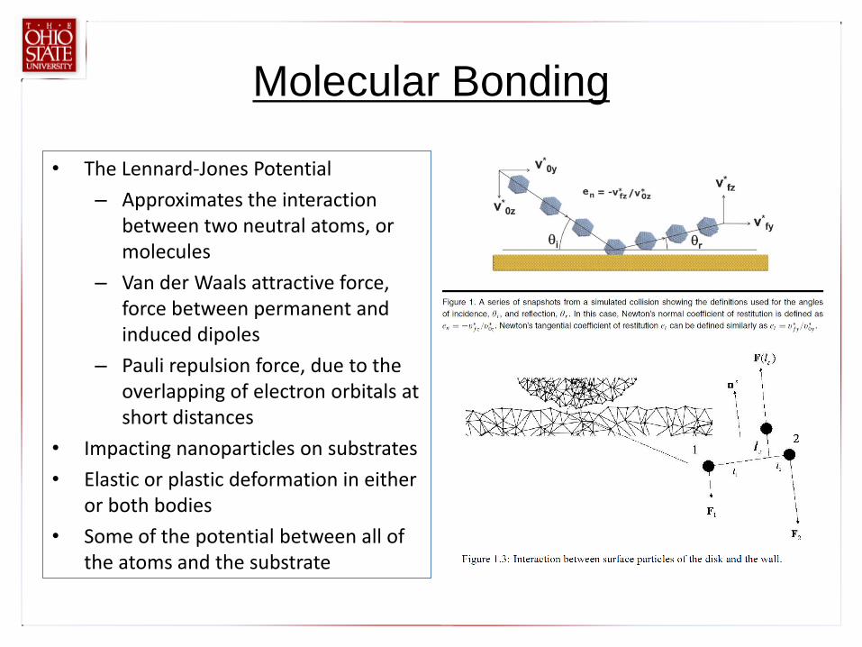
Molecular Bonding
• The Lennard-Jones Potential
– Approximates the interaction between two neutral atoms, or molecules
– Van der Waals attractive force, force between permanent and induced dipoles
– Pauli repulsion force, due to the overlapping of electron orbitals at short distances
• Impacting nanoparticles on substrates
• Elastic or plastic deformation in either or both bodies
• Some of the potential between all of the atoms and the substrate

Molecular Bonding
• Technique is sensitive to the parameters desired for the deposition model
– Temperature
– Size
– Mass
– Velocity
– Impingement Angle
– Properties of the particle and surface
• Technique includes adhesion
• Technique must be solved for each individual case of particle impacting on surface
– Requires detailed data on the composition and structure of both the particulate and the surface
– Many cases need to be calculated in order to form an empirical relation

FEM
• Model by Thornton Johnson and Gilabert
– Uses the mesh of the particle and the substrate
– Inputs require the material properties of the particle and the substrate
– Outputs the initial and final kinetic energy of the particle
• Elastoplastic deformation of both the particle and the substrate

FEM
• Technique is sensitive to the parameters desired for the deposition model
– Temperature
– Size
– Mass
– Velocity
– Impingement Angle
– Properties of the particle and surface
• Technique includes adhesion
• Technique must be solved for each individual case of particle impacting on surface
– Requires detailed data of the stress-strain relationship of the particulate and the substrate at varying temperature
– This data can only be acquired through experimental data and empirical relations
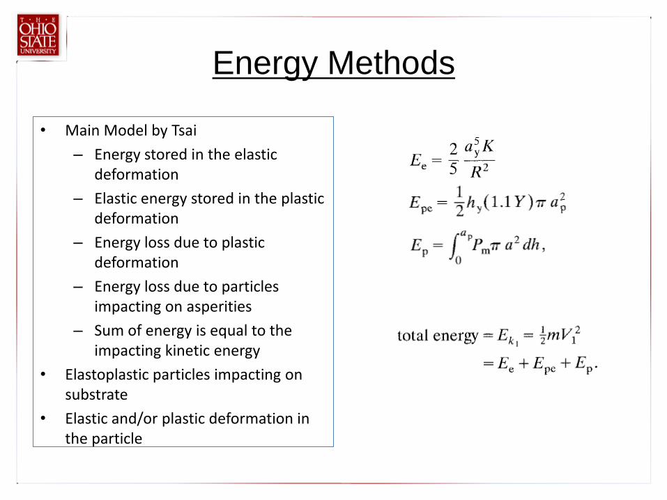
Energy Methods
• Main Model by Tsai
– Energy stored in the elastic deformation
– Elastic energy stored in the plastic deformation
– Energy loss due to plastic deformation
– Energy loss due to particles impacting on asperities
– Sum of energy is equal to the impacting kinetic energy
• Elastoplastic particles impacting on substrate
• Elastic and/or plastic deformation in the particle

Energy Methods
• Technique is sensitive to the parameters desired for the deposition model
– Temperature
– Size
– Mass
– Velocity
– Electrical charging
– Properties of the particle and surface
– Roughness
• Technique includes adhesion
• Calculations can easily be made for each impacting particle
– Requires detailed data of the stress-strain relationship of the particulate and the substrate at varying temperature
– This data can only be acquired through experimental data and empirical relations

Yield Stress Determination
• Models by Green and Thornton
– Calculates the energy stored elastically in the body
– Determines point of plastic deformation from the Von Misesimpact criteria
– Work done by plastic deformation is calculated
– Uses the residual interference and the Hertzian model to calculate restitution
– Adhesion is considered in some models
• Valid only for elastic perfectly plastic particles impacting on substrate
• Elastic and/or plastic deformation in the particle

Yield Stress Determination
• Technique is sensitive to the parameters desired for the deposition model
– Temperature
– Size
– Mass
– Velocity
– Oblique Impacts
– Properties of the particle and surface
• Some variations include adhesion
• Calculations can easily be made for each impacting particle
– Requires the data for yield stress
– This data can be acquired through experimentation or empirical modeling

Elastoviscoplasticity
• Model by Adams
– Dependent on the mean pressure which is obtained from the flow stress corresponding to the strain rate
– Uses the mean strain rate
– Plastic loading
– Herschel-Bulkley materials
– Small amount of elastic strain
– Does not include adhesion
• Model by Fu
– Yield stress of impacting particle is dependent on the strain rate of the particle
– Uses Herschel-Bulkley viscoplasticrelationship to determine the modified yield stress
– Linear elastic behavior

Desired Model
• Energy Methods– Temperature
– Size
– Mass
– Velocity
– Electrical charging
– Properties of the surface
– Roughness
• Yield Stress– Temperature
– Size
– Mass
– Velocity
– Oblique Impacts
– Properties of the surface
• Energy method appears to be optimal model
• Complexity of determining Stress vs. Strain as a f(T)
• Yield stress is elastic perfectly plastic
• Easier to implement
• Only requires yield stress
• Can be combined with the energy loss from roughness
• Elastoviscoplasticity model can account for stress flow and strain rates during plastic deformation
• Elastoviscoplasticity– Temperature
– Size
– Mass
– Velocity
– Properties of the surface

Desired Model- The Different Pieces
• Energy Methods
– Complicated Stress vs. Strain relationship
– Includes Adhesion
– Roughness
– Electrostatic forces
• Yield Stress
– Elastic perfectly plastic materials
– Thornton
• Adhesion
• Constant surface energy
– Green
• No Adhesion
• Application of Hertzianpressure distribution
• Elastoviscoplasticity models
• Effects of strain rates on the yield stress
• No Elastic Behavior
• Incorporation of the consistency and plastic flow index

82

Supplementary Slides
83

84
• Viscosity-Temperature relationship is necessary
• Model of Senior et. al.
–Uses coal ash chemical composition
– Ash is made up of a Silicate melt with a network
of SiO44+
• Three categories of cations that interact with
network
–Glass formers - Si4+, Ti4+, and P5+
– Modifiers - Ca2+, Mg2+, Fe2+, K+ and Na+
– Amphoterics - Al3+, Fe3+, and B3+
ViscosityTemp. Relation

Flow Physics
• Flow solution using FLUENT
– Commercially available
– Solves discretized flow equations to predict fluid dynamics
• Deposition Models
– developed in C language and incorporated as User-Defined Functions in Fluent
• Turbine grid made using GridPro
– VKI Turbine Vane
– GE-E3 Turbine Vane
85
VKI Turbine Vane (2D)
E3 Turbine Vane (3D)