Embed Size (px)
Citation preview

Effects of Free Stream Turbulence on
Compressor Cascade Performance
Justin W. Douglas
Thesis submitted to the Faculty of the Virginia Polytechnic Institute and
State University in partial fulfillment of the requirements for the degree of
Master of Science
In
Mechanical Engineering
Committee:
Dr. Wing Fai Ng, Chair
Dr. Clint Dancey
Dr. Thomas Diller
Dr. Shiming Li
March 1, 2001
Blacksburg, VA
Keywords: Turbulence Grid, Boundary Layer Transition, Aerodynamic Loss, Compressor Cascade, Hotwire, Anemometer
Copyright 2000, Justin W. Douglas
II
Effects of Free Stream Turbulence on Compressor Cascade Performance
Justin W. Douglas
(ABSTRACT)
The effects of grid generated free-stream turbulence on compressor cascade performance was
measured experimentally in the Virginia Tech blow-down wind tunnel. The parameter of key
interest was the behavior of the measured total pressure loss coefficient with and without
generated free-stream turbulence. A staggered cascade of nine airfoils was tested at a range of
Mach numbers between 0.59 and 0.88. The airfoils were tested at both the lowest loss level
cascade angle and extreme positive and negative cascade angles about this condition. The
cascade was tested in a Reynolds number range based on the chord length of approximately 1.2-
2x10⁶. A passive turbulent grid was used as the turbulence-generating device, it produced a
turbulent intensity of approximately 1.6%. The total pressure loss coefficient was reduced by
11-56% at both the �lowest loss level� and more positive cascade angles for both high and low
Mach numbers. Oil Visualization and blade static pressure measurements were performed in
order to gain a qualitative understanding of the loss reduction mechanism. The results indicate
that the effectiveness of an increasing turbulent free-stream on loss reduction, at transonic Mach
numbers, depends on whether the shock wave on the suction surface is strong enough to
completely separate the boundary layer. At negative cascade angles, increasing free-stream
turbulence proved to have a negligible influence on the pressure loss coefficient. At cascade
angles where transition exists within a laminar separation bubble, increasing free-stream
turbulence suppressed the extent of the laminar separation bubble and led to an earlier turbulent
reattachment.

III
ACKNOLEDGEMENTS
I would like to thank God for giving me the opportunity and the ability to obtain a Master�s
Degree. I would also like to thank Dr. Wing Ng for allowing me to conduct this research and for
his patience and advice during a very trying project. Dr. Clint Dancey, Dr. Karen Thole, Dr. Joe
Schetz, and Dr. Tom Diller, thank you for always allowing me to march into your offices with
various questions at all hours of the day and night for advice on the subject of turbulence.
A special thanks to Dr. Shiming Li for all of the long hours of experiments in both successful
and frustrating outcomes, you always showed great patience and encouragement. Your advice
and guidance both on this project and the art of fishing have proved to be tremendously helpful.
I would also like to thank Casey Carter, Bo Song, Todd Bailie, and Tom Vandeputte for their
willingness to assist me with my experiments in any way that I needed. I would also like to
thank Greg, Kurt, Bruce, Jamie, Bill, and Timmy, from both the AOE and ME machine shop for
all of their valuable advice on machining issues. A special thanks to Dr. Michael Sexton for
sparking the interests of a young cadet in the field of Turbomachinery, it inspired me to pursue
this masters degree.
Finally, I would like to thank my fiancée, Marcia James, for supporting me both through the
grueling years at the Virginia Military Institute and through Virginia Tech. For your love and
support I am forever grateful. Special thanks to my parents, James Douglas and Jacqueline
Crider for instilling in me that the only way to accomplish success is through hard work.
�...Times like these try men�s souls.� Thomas Paine

IV
TABLE OF CONTENTS
TABLE OF CONTENTS ........................................................................................................... IV
TABLE OF FIGURES................................................................................................................VI
INDEX OF TABLES ................................................................................................................ VII
NOMENCLATURE.................................................................................................................VIII
I Cascade Angle, Degrees................................................................................................VIII
CHAPTER 1 INTRODUCTION................................................................................................. 1
1.1 BACKGROUND AND PREVIOUS RESEARCH .......................................................................... 3
1.1.1 Effects of Free-Stream Turbulence on Boundary Layer Transition ........................... 3
1.1.2 Effects of Incidence on Boundary Layer Transition and Separation.......................... 6
1.1.3 The Effect of Free-Stream Turbulence on the Loss Coefficient .................................. 9
1.2 OBJECTIVE OF THE CURRENT WORK................................................................................. 11
CHAPTER 2 EXPERIMENTAL METHOD ........................................................................... 12
2.1 DESCRIPTION OF CASCADE ............................................................................................... 12
2.2 DESCRIPTION OF TURBULENCE GRID DESIGN................................................................... 15
2.2.1 Turbulence Decay Model.......................................................................................... 15
2.2.2 Sizing of Bars and Mesh ........................................................................................... 16
2.2.3 Position of Turbulence Grid ..................................................................................... 20
2.2.4 Prediction of Wake Width and Mixing Point ............................................................ 21
2.3 THE WIND TUNNEL FACILITY........................................................................................... 25
2.4 DESCRIPTION OF INSTRUMENTATION AND DATA ACQUISITION ........................................ 28
2.4.1 Upstream and Downstream Total and Static Pressure Measurements .................... 28
2.4.2 Hot Wire Setup and Measurements........................................................................... 34
2.4.3 Static Pressure Measurements on the Blade Surface ............................................... 37
2.5 OIL FLOW VISUALIZATION ............................................................................................... 38

V
2.6 DATA REDUCTION ............................................................................................................ 39
2.6.1 Pressure Loss Coefficient ......................................................................................... 39
2.6.2 One-Calibration and Turbulence Intensity ............................................................... 42
CHAPTER 3 EXPERIMENTAL RESULTS AND DISCUSSION........................................ 47
3.1 TURBULENCE LEVEL MEASUREMENTS ............................................................................. 47
3.2 AERODYNAMIC DATA REGARDING PERFORMANCE AND THE BOUNDARY LAYER ............ 50
3.2.1 Total Pressure Loss Coefficient ................................................................................ 50
3.2.1.1 Effects of Turbulence on the Loss Coefficient at Negative Cascade Angles ........ 52
3.2.1.1 Effects of Turbulence on the Loss Coefficient at Positive Cascade Angles ......... 55
3.2.2 Isentropic Mach-Number Distribution on the Blade Surface ................................... 63
CHAPTER 4 CONCLUSIONS AND RECOMMENDATIONS ........................................... 74
REFERENCES............................................................................................................................ 76
APPENDIX A UNCERTAINITY ANALYSIS ....................................................................... 78
APPENDIX B DOWNSTREAM LOSSES AND M2 VS PITCH.......................................... 80
APPENDIX C HOT WIRE CALIBRATION AND REDUCTION CODE.......................... 82
Hot-wire calibration theory ............................................................................................. 82
One point calibration methodology ................................................................................. 83
APPENDIX D REDUCTION CODE FOR TURBULENCE SCALE .................................. 88
VITA............................................................................................................................................. 90
VI
TABLE OF FIGURES
FIGURE 2. 1 SCHEMATIC OF STATOR GEOMETRY .........................................................................................................13
FIGURE 2. 2 ASSEMBLED COMPRESSOR CASCADE .......................................................................................................14
FIGURE 2. 3 PHOTOGRAPH OF TURBULENT GRID .........................................................................................................18
FIGURE 2. 4 SCHEMATIC OF TURBULENCE GRID .........................................................................................................19
FIGURE 2. 5 POSITION OF TURBULENCE GRID ..............................................................................................................20
FIGURE 2. 6 WAKE FROM SINGLE BAR (SCHETZ,1993) ................................................................................................21
FIGURE 2. 7 UPSTREAM TOTAL PRESSURE TRAVERSE .................................................................................................23
FIGURE 2. 8 UPSTREAM TRAVERSE ASSEMBLY............................................................................................................24
FIGURE 2. 9 VIRGINIA TECH TRANSONIC WIND TUNNEL .............................................................................................26
FIGURE 2. 10 SCHEMATIC OF LOW SPEED DATA ACQUISITION ....................................................................................33
FIGURE 2. 11 SCHEMATIC OF HIGH SPEED DATA ACQUISITION WITH HOT WIRE.........................................................36
FIGURE 2. 12 INSTRUMENTED STATIC PRESSURE STATORS..........................................................................................37
FIGURE 2. 13 OIL VISUALIZATION ENTIRE CASCADE...................................................................................................38
FIGURE 2. 14 MEASURED CENTER PASSAGES ..............................................................................................................39
FIGURE 3. 1 HW VOLTAGE PLOTS FOR RESPECTIVE TU INTENSITIES ..........................................................................48
FIGURE 3. 2 LOSS COEFFICIENT VS. INCIDENCE FOR INLET MACH NUMBERS 0.60, 0.65, 0.70, 0.75............................51
FIGURE 3. 3 LOSS COEFFICIENT VS. INCIDENCE FOR INLET MACH NUMBERS 0.80, 0.85..............................................52
FIGURE 3. 4 OIL VISUALIZATION, I=44.4O, M1~0.65 ...................................................................................................53
FIGURE 3. 5 LOSS VS M1; I=44.4O FIGURE 3. 6 LOSS VS M1; I=48.4O ...................................................................55
FIGURE 3. 7 LOSS LEVEL COMPARISON(CARTER,2001) ...............................................................................................58
FIGURE 3. 8 EFFECT OF TU ON LOSSES AND DEVIATION ANGLE(EVANS,1985)............................................................59
FIGURE 3. 9 LOSS VS. RE(CITAVY,1977) FIGURE 3. 10 LOSS VS. RE(CITAVY,1977)...............................................61
FIGURE 3. 11 ISENTROPIC MACH NUMBER DISTRIBUTION I=44.4O ..............................................................................63
FIGURE 3. 12 OIL VISUALIZATION CHOKED CONDITION ..............................................................................................64
FIGURE 3. 13 MOMENTUM AN DISPLACEMENT THICKNESS (EVANS,1985) ..................................................................65
FIGURE 3. 14 ISENTROPIC MACH NUMBER DISTRIBUTION I=48.4O ..............................................................................66
FIGURE 3. 15 OIL VISUALIZATION 48.4O NO TU FIGURE 3. 16 OIL VISUALIZATION 48.4O WITHT U ..............67
FIGURE 3. 17 TRANSITION VS B1 (STEINERT,1996) FIGURE 3. 18 TRANSITION VS M1 (STEINERT,1996) ............69
FIGURE 3. 19 MACH NUMBER DISTRIBUTION (STEINERT,1996)...................................................................................71
FIGURE 3. 20 MISES PREDICTION(SCHREIBER,2000)..................................................................................................72

VII
FIGURE B. 1: SAMPLE OF DOWNSTREAM LOSS AND M2 PROFILES .............................................................................80
FIGURE B. 2 LOSS VS INLET MACH NUMBER ...............................................................................................................81
INDEX OF TABLES
TABLE 2. 1 BLADE SPECIFICATIONS, MINIMUM LOSS CONDITION ...............................................................................13 TABLE 3. 1 COMPARISON BETWEEN PREDICTED AND MEASURED TU INTENSITY ........................................................49 TABLE 3. 2 SUMMARY OF LOSS REDUCTION ................................................................................................................56 TABLE A. 1: BIAS ERRORS DUE TO INSTRUMENTATION AND UNCERTAINTY. ..............................................................78 TABLE A. 2: MAXIMUM PROPAGATED UNCERTAINTY. ................................................................................................79

VIII
NOMENCLATURE
LE Leading Edge of Stator
TE Trailing Edge of Stator
SS Suction Side of Stator
I Cascade Angle, Degrees
Ms Isentropic Mach Number
x/c Percentage Chord
M1 Inlet Mach Number
M2 Exit Mach Number
Tt1 Total Temperature, Upstream
Ts1 Static Temperature, Upstream
Pt1 Total Pressure, Upstream of Grid
Pt1cas Total Pressure, Upstream of Cascade, Downstream of Grid
Ps1 Static Pressure, Upstream
Ps2 Static Pressure, Downstream
Pt2 Total Pressure, Downstream
dPt Differential Total Pressure
Re Reynolds Number Based on Chord
Tu Turbulence Intensity
r Density
g Gamma=1.4, Cold-Air Standard
w Pressure Loss Coefficient
m Viscosity
a Inlet Cascade Angle
b Exit Metal Angle
C Blade Chord, or Calibration Constant for HW Calibration
t Pitch
x Axial Distance

IX
d diameter of bars in Turbulence Grid
M Mesh Size of Grid
R Gas Constant
U1 Instantaneous Velocity, Upstream
UA2 Axial Velocity, Downstream
UA1 Axial Velocity, Upstream
AVDR-Axial Velocity Density Ratio
CDA Controlled Diffusion Airfoil
PVD Prescribed Velocity Distribution Airfoil

1
Chapter 1 INTRODUCTION
In today�s ever-competitive gas turbine market, industry constantly strives for lower
aerodynamic losses at both design and off design conditions. In the twenty-first century not only
does industry feel pressure to lower losses to make their engines financially attractive, but also to
meet the ever tightening emissions standards from the federal government. The efficiency of a
gas turbine is largely dependent on its turbomachinery components. If engine designers are able
to improve the flow efficiency through both the compressor and turbine side of the gas turbine,
then less fuel must be added to obtain the higher levels of power that were once considered
unsatisfactory due to emissions or industry standards for efficiency. Therefore, the design of
blade profiles and the manipulation of the flow over these blade profiles in order to improve
aerodynamic efficiency are of utmost importance. For example, when impingement cooling of
turbine blades was introduced to industry the efficiency of the gas turbine cycle increased due to
the capacity to run the turbine at higher inlet temperatures. The idea of fogging a compressor, or
spraying water droplets into the inlet of an engine, in order to use evaporative cooling to achieve
higher compression efficiency, is also being researched in this area.
The stators and rotors that make up the numerous stages of a compressor are designed to operate
at a certain optimal condition, usually referred to as the design point. However, during their
actual application they are operated at off design conditions as well. In these off design ranges
the flow enters the stator and rotor stages at varying incidence angles, and lower losses are even
more difficult to achieve due to certain flow phenomena such as flow separation and shock
waves. These phenomena act to drive the losses to higher levels and eventually cause compressor

2
stall. Unlike turbines, the efficiency of a compressor is very sensitive to inlet incidence angle
change due to the diffusing of the flow and the creation of an adverse pressure gradient. When
the flow separates due to an adverse pressure gradient, the blade profile loss is dependent on the
extent of the flow separation. The use of increased free-stream turbulence plays a role in
manipulating this flow separation, and ultimately the performance of the compressor stage.
For years, researchers around the world have used cascade tests to conduct research and to push
the envelope for running turbomachines at off design conditions. Although these cascade tests
are not a perfect model representation of an actual rotating turbomachine, cascade testing
provides the blade designer with a more economical and experimentally simpler method of
examining the aerodynamic performance under various operating conditions. Cascade testing is
also used for validation of computational fluid dynamic (CFD) flow solvers. These CFD
programs are generally pretty accurate in predicting aerodynamic losses for subsonic flow unless
flow phenomena such as shock waves or laminar separation are underestimated near transonic
Mach numbers. Since new flow solvers are frequently being programmed and tweaked by
industry, cascade testing is still a reliable method for determining the actual aerodynamic loss of
a blade profile.

3
1.1 Background and Previous Research
Since cascade testing has evolved into an effective model for the testing of compressor blades,
the parameters that control testing conditions have also changed over the years. It is common
practice to find that wind tunnels around the country are designed for very low inlet turbulence
levels. The advantage for designing a wind tunnel in this way is that it provides a good baseline
for cascade experiments and presents the possibility to raise the turbulence level to a desired
level in a controlled fashion. Now, common wind tunnel practice and actual gas turbine
operation have raised the question of whether cascade testing without a suitable free-stream
turbulence level is reliable, due to the turbulent rotor wakes internal to the engine. Gostelow
(1984) believes that cascade results obtained without a suitable turbulence generating device are
quite suspect.
1.1.1 Effects of Free-Stream Turbulence on Boundary Layer Transition
The generation of free-stream turbulence changes the characteristics of transition of the boundary
layer on the suction surface of turbomachinery blades. Quantitatively, this transition point
movement has been studied for years, but with the constant improvement of visualization
techniques it is possible for these effects to be seen qualitatively. Work by Mayle (1991), Evans
(1971), and Schreiber (2000) have extensively researched and eloquently documented the effects
of turbulence on boundary layer transition.
Mayle (1991) gives a detailed description of the importance of understanding the role of
boundary layer transition in a gas turbine. He defines four modes of transition characteristic to
flow through the various stages of a gas turbine engine. The first mode is one of natural

4
transition, which begins with the formation of weak instabilities, or TS (Tollmien and
Schlichting) waves, in the laminar boundary layer, followed by the development of larger
instabilities, which eventually lead to fully turbulent flow. The second mode is called �bypass�
transition and is characterized by the skipping of the TS instabilities with procession to fully
turbulent flow. He points out that bypass transition is caused by large disturbances in the
external flow, such as free stream turbulence. The turbulence spots that develop in the later
stages of natural transition, just before fully turbulent flow, are present within the boundary layer
without the TS wave procession and are caused by the large fluctuations impinged on the blade
surface due to free-stream turbulence (Mayle,2001). The third mode of transition is one of
locally separated laminar flow that is contained within a bubble, known as the laminar separation
bubble. Mayle describes this transition as one that may occur in the free shear layer, like flow
near the surface, and in this case the flow may reattach as a turbulent flow. He suggests that this
type of transition can occur in an adverse pressure gradient, and that a method of making this
bubble as short as possible is an effective control to improve performance. Lastly, he points out
that for transonic airfoils wake-induced transition is observed and is characterized as periodic-
unsteady transition. He summarizes this form of transition induced by wakes or trailing shocks
from upstream rotors to be so disruptive to the laminar boundary layer that the turbulent spots
form immediately and coalesce into a turbulent strip that grows as it propagates downstream.
The first three modes described above are easily understood in two dimensions, the fourth mode
is completely a three dimensional effect, where more than one of the modes of transition can
exist on the blade surface at one time, or multi-mode transition. Concerning strictly the notion of
turbulence, Mayle made several distinct conclusions. First is that transition is dominated mainly
5
by the free-stream turbulence, pressure gradient, and the periodic unsteady passing of wakes.
Second, onset of transition is significantly dependent upon free stream turbulence both intensity
and scale. Next, he concludes that the effects of surface roughness, surface curvature,
compressibility, and heat transfer on transition are secondary to those of free-stream turbulence.
Lastly, the length of transition depends only on the turbulence level and the pressure gradient
(Mayle,2000).
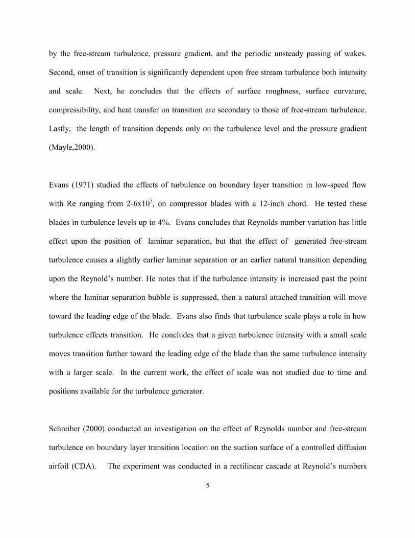
Evans (1971) studied the effects of turbulence on boundary layer transition in low-speed flow
with Re ranging from 2-6x10⁵, on compressor blades with a 12-inch chord. He tested these
blades in turbulence levels up to 4%. Evans concludes that Reynolds number variation has little
effect upon the position of laminar separation, but that the effect of generated free-stream
turbulence causes a slightly earlier laminar separation or an earlier natural transition depending
upon the Reynold�s number. He notes that if the turbulence intensity is increased past the point
where the laminar separation bubble is suppressed, then a natural attached transition will move
toward the leading edge of the blade. Evans also finds that turbulence scale plays a role in how
turbulence effects transition. He concludes that a given turbulence intensity with a small scale
moves transition farther toward the leading edge of the blade than the same turbulence intensity
with a larger scale. In the current work, the effect of scale was not studied due to time and
positions available for the turbulence generator.
Schreiber (2000) conducted an investigation on the effect of Reynolds number and free-stream
turbulence on boundary layer transition location on the suction surface of a controlled diffusion
airfoil (CDA). The experiment was conducted in a rectilinear cascade at Reynold�s numbers

6
ranging from 0.7-3.0x10⁶ and turbulence intensities from 0.7 to 4%. Two flow visualization
techniques were used in this experiment. For low speed tests oil visualization was used, but at
high speeds the oil visualization was found to be less sensitive to skin friction discontinuities. In
order to better visualize boundary layer phenomena at high Reynold�s numbers, Schreiber used a
liquid crystal technique that distinguishes differences in adiabatic wall temperatures. At small
turbulence intensities (Tu<3%) and all Reynolds numbers tested, Schreiber finds that the
accelerated front portion of the blade is laminar and that transition occurs within a laminar
separation bubble shortly after the maximum velocity, which was found near 35-40% chord.
Conversely, at turbulence higher than this range and high Reynold�s numbers, Schreiber
observes that transition propagates upstream into the accelerated front region of the blade. In
this case Schreiber describes this moved transition mode at high Reynold�s number and high
turbulence level as a bypass mode, or one where the laminar separation bubble is not visible.
Schreiber points out that testing between turbulence levels of 2-4%, transition onset location is
most dependent on the Reynolds number. Schreiber concludes that surface roughness may also
play a role in the movement of transition and should be examined in future research.
1.1.2 Effects of Incidence on Boundary Layer Transition and Separation
In order to examine the full background of the current research, it is important to look at all
aspects that contribute to the development of boundary layers. The above authors have carried
out very detailed investigations on the effects of turbulence on the characteristics of boundary
layers, but stator incidence also plays a role in determining transition and separation of boundary
layers. Work by Steinert (1994) has documented the effect of incidence on boundary layer
behavior, and in turn, how this behavior influences the pressure loss coefficient for the given
blade profile.

7
Steinert (1996) conducts a study using the liquid crystal visualization technique to examine
transition, local separation, and complete separation at design and off-design of a controlled
diffusion airfoil (CDA). The CDA�s were designed for an inlet Mach number of 0.62, and with a
total flow turning of 27.6o. A total of seven blades were tested, with a chord of 70mm, and two
blades instrumented with 10 static pressure taps on the suction and pressure sides of the blades,
respectively. The chord Reynolds number at design was 8x10⁵ and the free-stream turbulence
level was 2.5%. It should be noted, that all tests conducted were with a constant turbulence
level so the effects of varying turbulence level at different incidence angles is not represented in
his work. However, assuming the turbulence level in Schreiber�s work as a baseline, valuable
boundary layer behavior and loss coefficient trends can be observed from his experiments.
Steinert describes the importance of surveying the whole blade surface and not only point-by-
point measurements, because both transition and separation are three-dimensional even in a
linear cascade.
Steinert first examines the effect of incidence on boundary layer transition at constant inlet Mach
number. Steinert reported that a range of plus or minus 4o incidence of the design point that the
boundary layer behavior on the suction side of the airfoil was almost identical with a laminar
separation bubble at about 42-51% chord with turbulent reattachment. He notes at negative
incidences that the separation bubble moves slightly downstream. At the incident angle of about
plus 5o, the laminar separation bubble vanished and transition moved to about 22% chord with
complete separation at about 60% chord. An additional increase in incidence of one degree,
shows that transition moves to 10% chord and then separates at about 50-55% chord. He
describes this transition as somewhat unsteady, so the author assumes this is a bypass transition

8
mode. On the pressure side Steinert reports that transition occurred at around 20-23% chord,
except at extreme negative incidence a small separation bubble was observed around 3% chord
due to a shock wave caused by the expansion around the leading edge of the airfoil. Steinert�s
most interesting findings were when the inlet Mach number was varied and a loss profile was
given as a function of inlet Mach number for design, positive, and negative incidence. At design,
he describes the boundary layer transition to consist within a laminar separation bubble at around
40-50% chord with turbulent reattachment up to an inlet Mach number of 0.79. At transonic
Mach numbers above this point, he reports a slight movement forward of the transition point
followed by complete laminar separation. He concludes that this separation is probably caused
by a lambda shock system interacting with the boundary layer, that in turn, results in complete
separation. He supports this theory with the calculation of the respective supersonic isentropic
Mach numbers on the blade surface in the accelerated front portion of the airfoil. At transonic
Mach numbers he documents a steep increase in the loss coefficient. At negative incidence he
notices that this choking and separation of the boundary layer first appears at an inlet Mach
number of 0.626. At positive incidence of higher than plus 4o, he described the cascade as again
being in a choked state and with increasing inlet Mach number the losses increase very sharply
as the flow is completely separated. Steinert mentions in conclusion that the Axial Velocity
Density Ratio (AVDR), has a common inversely proportional effect on the loss coefficient. This
may be better explained as the tendency of losses to decrease with increasing AVDR and flow
turning. The AVDR may also be defined as a measure of the two-dimensionality of the flow.
The AVDR is varied between 0.98 and 1.15 in Steinert�s research.

9
1.1.3 The Effect of Free-Stream Turbulence on the Loss Coefficient
The final perspective in studying the background for the present work is to examine previous
literature for documentation of the direct effect of free-stream turbulence on the calculated
pressure-loss coefficient through a compressor cascade. Finding a substantial amount of relevant
work that documents the direct effect of turbulence on the loss coefficient is somewhat difficult,
work by Evans (1985) and Citavy (1977) provide some direct insight to this phenomena.
Evans (1985) performed boundary layer, pressure loss, skin friction, and deviation angle
measurements in the presence of varying free stream turbulence on a cascade of compressor
blades that had a 1 foot measured chord. The experiments were conducted in turbulent free
streams at intensities of 0.68%, 3.14%, and 5.2%, and a constant Reynolds number of 5x10⁵.
The angle of attack tested was at plus 4o of the design incidence. The blades were designed for
43.35o total turning, and a solidity ratio of 0.709. Agreeing with other researchers� results, Evans
found that at increased turbulence levels the laminar separation bubble will shorten, and
eventually collapse. Even higher turbulence levels caused the transition point to move towards
the leading edge of the blade (Evans,1985). Evans conducted boundary layer measurements at
30%, 50%, 70%, and 80% chord on the suction surface of the blade to observe the characteristics
of the boundary layer under varying degrees of turbulence. Evans found that with increasing
turbulence the momentum thickness decreased, which in turn, signifies an increasing velocity
profile thickness. At chord-wise locations close to the separation point momentum thickness
tends to increase with increasing turbulence below 3%. At turbulence levels above 3% the effect
of an increased velocity profile fullness again becomes dominant even near separation and
momentum thickness again tends to decrease. Evans reports that at all values of the adverse
10
pressure gradient, skin friction is seen to increase with increasing free-stream turbulence, which
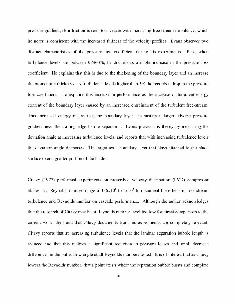
he notes is consistent with the increased fullness of the velocity profiles. Evans observes two
distinct characteristics of the pressure loss coefficient during his experiments. First, when
turbulence levels are between 0.68-3%, he documents a slight increase in the pressure loss
coefficient. He explains that this is due to the thickening of the boundary layer and an increase
the momentum thickness. At turbulence levels higher than 3%, he records a drop in the pressure
loss coefficient. He explains this increase in performance as the increase of turbulent energy
content of the boundary layer caused by an increased entrainment of the turbulent free-stream.
This increased energy means that the boundary layer can sustain a larger adverse pressure
gradient near the trailing edge before separation. Evans proves this theory by measuring the
deviation angle at increasing turbulence levels, and reports that with increasing turbulence levels
the deviation angle decreases. This signifies a boundary layer that stays attached to the blade
surface over a greater portion of the blade.
Citavy (1977) performed experiments on prescribed velocity distribution (PVD) compressor
blades in a Reynolds number range of 0.6x10⁵ to 2x10⁵ to document the effects of free stream
turbulence and Reynolds number on cascade performance. Although the author acknowledges
that the research of Citavy may be at Reynolds number level too low for direct comparison to the
current work, the trend that Citavy documents from his experiments are completely relevant.
Citavy reports that at increasing turbulence levels that the laminar separation bubble length is
reduced and that this realizes a significant reduction in pressure losses and small decrease
differences in the outlet flow angle at all Reynolds numbers tested. It is of interest that as Citavy
lowers the Reynolds number, that a point exists where the separation bubble bursts and complete

11
separation with reattachment is observed. The influence of free-stream turbulence lowers this
bursting Reynolds number significantly from his baseline testing. It is also apparent at these
Reynolds numbers close to the bursting state, that the outlet flow angle is most sensitive to free-
stream turbulence.
1.2 Objective of the Current Work
The current work hopes to attempt to bring most of the previous research together and examines
the effects of free-stream turbulence on the pressure loss coefficient at varying degrees of
incidence and varying inlet Mach numbers. Once this effect is determined quantitatively, in
terms of the calculated pressure loss coefficient, then the author would like to try and explain
these effects somewhat qualitatively by the use of oil visualization and static pressure data
obtained from the respective suction and pressure sides of the airfoil. The current work
compares data from a baseline case, with low levels of free-stream turbulence, to that of a
turbulence-generated free-stream. All inlet conditions were held constant between the two
phases of the experiment to provide a detailed effect, if any, of free stream turbulence on the
performance of the compressor cascade. In conclusion, the author will compare the experimental
results with that of previous literature to analyze, reinforce, and discuss the validity of these
results.

12
Chapter 2 EXPERIMENTAL METHOD
The following chapter is a description of the experimental setup in the laboratory. Section 2.1
describes the cascade design and capability. Section 2.2 gives a detailed description of the
design of the turbulence grids. Section 2.3 describes the wind tunnel facility. Section 2.4
describes the instrumentation and data acquisition techniques used in the current experiment.
Section 2.5 describes the flow visualization techniques used for baseline testing, while 2.6
describe the data reduction procedures and techniques.
2.1 Description of Cascade
The test section used for this research consisted of a nine-blade, 2-D, linear, compressor stator
cascade contained within two Plexiglas sidewalls. This set-up formed eight complete passages,
however, only the two middle passages were used for the recording and documentation of data.
The cascade can be tested at a 24 o inlet cascade angle range, a1. The stators are designed to be
used in a gas turbine engine. Table 2.1 summarizes the geometric properties of the compressor
cascade. Figure 2.1 and Figure 2.2, show a schematic of the turning on each blade, and a picture
of the assembled cascade, respectively.

ab = -6.8 o
1 = 44.4o
13
Figure 2. 1 Schematic of Stator Geometry
Table 2. 1 Blade Specifications, Minimum Loss Condition
Blade Chord, C 3.39 inches
Pitch, t 1.69 inches
Span 6 inches
Solidity 2.00
Inlet Cascade Angle, a1 44.4o
Exit Metal Angle, b -6.8 o
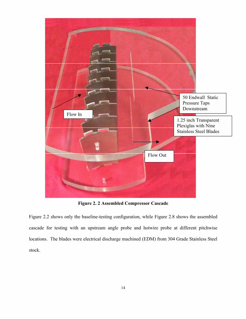
Figure 2.2 shows on
cascade for testing
locations. The blad
stock.
50 Endwall Static Pressure Taps Downstream
F
low In14
Figure 2. 2 Assembled Compressor Cascade
ly the baseline-testing configuration, while Figure 2.8 shows the assembled
with an upstream angle probe and hotwire probe at different pitchwise
es were electrical discharge machined (EDM) from 304 Grade Stainless Steel
1.25 inch Transparent Plexiglas with Nine Stainless Steel Blades
Flow Out

15
( )75
12.1−
= dxTu
2.2 Description of Turbulence Grid Design
This chapter describes all aspects of the design, position, and implementation of the turbulent
grid used in this experiment. It should be noted that two turbulent grids were designed and
tested, however due to a nonuniform upstream flow with the first iteration the results were
unreliable and the results discarded. The purpose of designing and implementing a turbulent grid
was to increase the free stream turbulence of the flow entering the cascade. Increasing this
turbulence level was hoped to lower the aerodynamic losses through the cascade by suppressing
or moving boundary layer transition closer to the leading edge of the stator. This movement or
suppression should force the flow to stay attached longer, thus increasing the aerodynamic
performance.
2.2.1 Turbulence Decay Model
According to normal grid theory for a round bar, square mesh grid (Roach, 1987), turbulence
intensity is given as
where d, is the bar diameter and x, is the axial dista
decay model for the design of the turbulence grid u
commonly known as the �5/7 Power Law. Roach
of Equation 2.1 such as:
( )75
80.0−
= dxTu
Equation 2. 1 (Roach,1987)n
s
gi
Equation 2. 2 (Baines,1951)
ce. Equation 2.2 was used as the primary
ed in this experiment. This relationship is
ves some important restrictions on the use

16
(1) The above equations are limited to the isotropic, or well developed region,
approximately 5 to 10 grid dimensions (mesh width) downstream of the grid
(Baines,1951)
(2) The inlet flow to the grid consist of a low turbulence level
(3) Grid must be normal to the flow
(4) The test section should be significantly large compare with the grid mesh width to
avoid sidewall boundary layer distortion
The notion of isotropic turbulence is that of developed turbulence that is unaffected by any
external force will only change according to its own decay. Turbulent flow fields that are
examined both near a wall and close to the turbulent source are not valid isotropic regions.
These flow fields are commonly referred to as anisotropic regions. Isotropic turbulence is
maintained by the energy cascade where larger eddies break up into smaller eddies and so on
until the smallest eddies are viscously dissipated (Holmberg,1996). The turbulence
measurements in this work were conducted 11.5 mesh widths, downstream of the turbulence grid
and at midspan of the test section. The baseline turbulence intensity to the entrance of the grid in
this experiment was measured to be approximately 0.1%. In this work the turbulence grid is
placed normal to the upstream flow and its position in the wind tunnel will be discussed in
further detail in Section 2.2.3. The size of the test section used for this work is 4.5 grid
dimensions, which is relatively small and therefore did not follow this theory as precisely as
expected.
2.2.2 Sizing of Bars and Mesh
Figure 2.3 shows a photograph of the turbulence grid used in this experiment, while Figure 2.4
shows a dimensioned schematic of the grid. The grid was designed in the form of a metal gasket

17
so that it could be easily swapped in and out of our tunnel without much disassembly or loss of
time. The plate and circular bars are both fabricated from common 1040 cold rolled steel stock.
The metal plate is 5/8 inch and the bars are 7/16 inch in diameter. In order to accommodate the
1/8 inch overhang of the bars on each side of the plate, they were milled down to 5/16 inch and
then welded into the plate. The bead formed by the weld was then grinded down flush with the
plate. Since the surface around the perimeter of the lattice of the grid is now smooth, a 1/16 inch
black rubber gasket was inserted on both sides of the grid to ensure a good seal. Figure 2.3
shows a photograph of the turbulence grid. It should be noted that on the reverse side of the
intersection of the bars the weld is not exposed to the flow in a way that would disrupt the wake
of the bar and the formation of turbulence. Figure 2.4 shows a schematic of the turbulence grid
so that the reader may get an idea of the general dimensions of the turbulence grid.

18
Figure 2. 3 Photograph of Turbulent Grid
The diameter of
leading edge of
the actual desig
intensity as a wo
this relationship,
use Baines� exp
Baines (1951) po
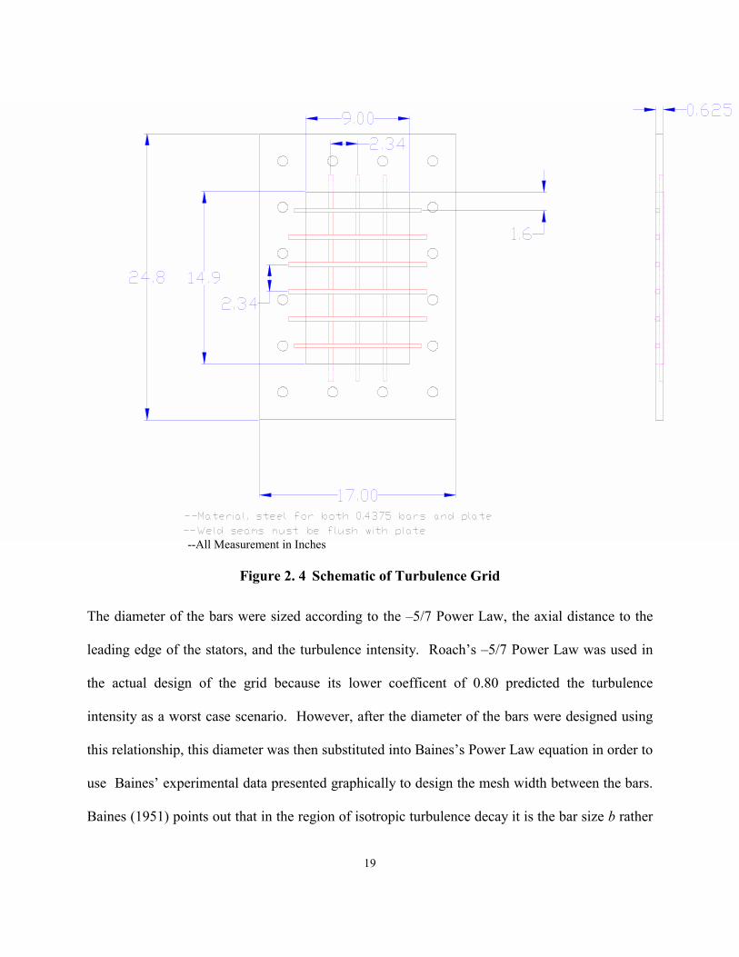
--All Measurement in Inches19
Figure 2. 4 Schematic of Turbulence Grid
the bars were sized according to the �5/7 Power Law, the axial distance to the
the stators, and the turbulence intensity. Roach�s �5/7 Power Law was used in
n of the grid because its lower coefficent of 0.80 predicted the turbulence
rst case scenario. However, after the diameter of the bars were designed using
this diameter was then substituted into Baines�s Power Law equation in order to
erimental data presented graphically to design the mesh width between the bars.
ints out that in the region of isotropic turbulence decay it is the bar size b rather

20
than the mesh size M that is the significant reference length. The mesh size used in the design of
the turbulence grid for this work was one that was chosen to be operable based on the the work
of Baines (1951), while the bar diameter was held as the design priority. The bars used in this
study were designed based on a turbulence intensity of 4.5% and due to Schreiber�s (2000)
discussion on boundary layer transition propagation. Schreiber explains that about 4-5%
turbulence intensity the boundary layer transition point propagates upstream to the front 10%
chord of the studied compressor blade. A detailed discussion and analysis of the measured
turbulence intensity and its effects on the flow will be included in Chapter 3 of this work.
2.2.3 Position of Turbulence Grid
Figure 2.5 shows the location of the turbulence grid within the test section and will allow the
reader to establish a reference to the compressor cascade.
Figure 2. 5 Position of Turbulence Grid

21
The centerline of the turbulence grid is 23 inches from the middle passage of the compressor
cascade. The reader may find it interesting that the grid is placed normal to a staggered cascade
due to previous studies with free stream turbulence generation the turbulence grid and cascade
are staggered at the same angle. However, due to the axial distance separating the grid and the
cascade, and the prediction of the turbulence decay used for this study, it was realistic to place
the grid normal to the staggered cascade. Since the grid was designed for an axial distance of 23
inches from the cascade, the turbulence decay is in its asymptotic decay region, so that an axial
distance within plus or minus four or five inches would be proportional to a negligible decay. In
other words, even though the cascade is staggered, each stator will see approximately the same
turbulence level.
2.2.4 Prediction of Wake Width and Mixing Point
Figure 2. 6 Wake from Single Bar (Schetz,1993)
Figure 2.6 (Schetz, 1993) shows a schematic of the variables examined in the prediction of a
wake from a single bar. The prediction of bar wake diffusion and the point where the wakes
begin to mix were very important in this work. It is important because if the wakes are detected
in the downstream pressure loss measurements the results could be confusing or misinterpreted.

22
In the first design iteration of the turbulence grid, the detection of the wakes of the bars just
upstream of the cascade, caused the downstream flow to be very aperiodic and thus the results
were unreliable. Wake flows from bars are made up of two regions, the near wake, right behind
the body, and the far wake. The near wake is complicated and often involves separated flows
and was not of interest for the design of the turbulent grid in this work (Schetz,1993). The point
of interest in this work was the momentum deficit, or far wake profile, at the axial distance
separating the turbulence grid with the leading edge of the stator passages to be examined. The
following equations were used to calculate the variables shown schematically in Figure 2.7
(Schetz,1993).
Where x is axial distance, CD, is the coefficient of d
velocity both at the centerline of the cylinder and
calculates what the width of the wake, b(x), at some a
from the centerline of the blunt body, in this case a c
was coupled with the other bars in the grid, separated
inches, the mixing point of the span-wise and pitch-w
for the reader to visualize the mixing from the horizo
will be located, however, the vertical bars are more c
that both the horizontal and vertical bars will have the
( ) ( )DCx Dxb ⋅⋅⋅= 21
57.0
⋅⋅=
∆
∞ xDC
UU DC
21
98.0
Equation 2. 3 (Schetz,1993)rag, D
free
xial d
ircula
by a
ise ba
ntal b
hallen
same
Equation 2. 4 (Schetz,1993)
, is the cylinder diameter, and U, is
-stream, respectively. Equation 2.3
istance x. This distance is measured
r bar. When this analysis of one bar
mesh dimension of approximately 2
rs could be predicted. It may be easy
ars and where the wake mixing point
ging to visualize. It should be noted
mixing point three dimensionally if

23
the mesh width is equal and symmetric throughout the grid. It was a priority to the design and
placement of the turbulent grid to know where this mixing point occurred and ensure that it was
a upstream of the cascade as soon as possible. Equation 2.4 predicts the momentum deficit in the
far wake profile. The closer the velocity ratio in Equation 2.4 is to unity, the more uniform the
upstream flow to the cascade becomes. The design of the turbulence grid ensured that the
mixing point was predicted to be as far upstream as possible to allow the bar wakes to have an
adequate mixing distance before entering the cascade. The author did not attempt to numerically
predict the momentum deficit in the mixing region upstream of the cascade. This momentum
deficit was determine experimentally by an upstream total pressure traverse performed at the
leading edge of the stators to be examined. The total pressure traverse proved to be uniform,
signifying that the wakes of the bars had sufficiently mixed. The total pressure traverse is shown
in Figure 2.7.
Upstream Total Pressure Distribution
0.8
0.9
1
1.1
0 1 2 3 4 5 6
Traverse Distance (inch)
Pt/P
t -ups
trea
m- o
f-Grid No Tu-Grid
New Tu-Grid
Figure 2. 7 Upstream Total Pressure Traverse

24
Figure 2.7 shows the total pressure measured at the leading edge of the middle cascade stator,
normalized by the total pressure upstream of the turbulence grid. The reader may expect a larger
pressure drop across the turbulence grid due to it size and blockage; however, since the grid is
located upstream of the convergent nozzle to the test section the velocity is relatively low.
Figure 2. 8 Upstream Traverse Asse
Hotwire/Total Pressure ProbeLocationsmbly

25
2.3 The Wind Tunnel Facility
The compressor cascade was tested in the transonic wind tunnel at Virginia Tech. The transonic
wind tunnel is a blow-down type of facility. The supply air is stored in two large storage located
on the outside of the laboratory and is pressurized by a four stage, reciprocating compressor. A
power control panel on the inside of the laboratory is used for control of the loading, unloading,
and activation of the blow-down sequence. Upon discharge from the storage tanks, the air is
cooled and passed through an activated-alumina dryer to dehumidify the air before entering the
wind tunnel. Although the dryer works to dehumidify the supply air, it is also necessary to drain
the condensation due to ambient air compression from each stage of the compressor every 10-12
consecutive tunnel runs. A pneumatically controlled butterfly-type control valve is fed by
pressurized reference air at 20psig and 80psig control air, and is used to maintain a constant inlet
total pressure to the test section. A personal computer is used to supply a voltage signal to an
electro-pneumatic converter that produces a proportionate output pressure based on the input
voltage from the computer. The voltage signal from the computer is described by seven
constants, among those constants is the inlet objective total pressure. The inlet objective total
pressure is varied to produce a range of different inlet Mach numbers to the test section.
Essentially, the tunnel computer uses feedback from the upstream total pressure probe to
maintain constant total pressure in the test section. After the air passes through the control valve,
it proceeds through a flow straightener and a meshed wire frame to provide uniform flow to the
test section. This meshed wire frame is located far enough upstream so that any turbulence
produced has decayed to an isotopic state and has an intensity of 0.1%. Typically, the valve
takes 5 seconds to attain steady inlet total pressure and then is able to sustain this pressure for up
to 15 seconds. Figure 2.9 shows a schematic of Virginia Tech�s blow-down wind tunnel facility.

26
Figure 2. 9 Virginia Tech Tran
Turbulence Grid
Upstream Total PressureProbe
Cascade/Test Section
sonic Wind Tunnel

27
The test section is fabricated with an aluminum frame with openings on each side for the
installation of the compressor cascade. The top and bottom aluminum blocks of the test section
form the top and bottom of the test section. The top and bottom blocks each have 0o entry and
51o, 60o exit angles, respectively. Plexiglas, 1.25 inches thick, encloses the compressor stator on
each side and make up the side wall of the flow region. The Plexiglas is held in place with 5
brass screw clamps on each side and a 12 inch C-clamp on top. The clamps support the test
section in a way that the compressor stators are visible from both sides of the assembled test
section. This visibility allows for optics-based flow visualization. The assembled Plexiglas
cascade is able to rotate freely inside of the aluminum test section so that a range of flow
incidence angles may be tested. The bottom block of the test section houses a smaller removable
block that allows the experimenter to insert a downstream probe for traversing the downstream
flow conditions. In this study, the removable block allowed for measurements at 50% chord
downstream of the trailing edge of the stators. The removable block was fabricated with 5
distinct probe holes that were machined at different angles so that when the cascade was tested at
off design angles the probe location would still maintain a traversing distance of 50% chord
downstream of the cascade. The unused probe locations were sealed with Allen screws when not
in use. The block allowed for an inlet incidence angle range of plus or minus 12o from design.

28
2.4 Description of Instrumentation and Data Acquisition
This section describes the instrumentation involved in examination of aerodynamic losses,
turbulence intensity, and location of suction and pressure side flow separation.
2.4.1 Upstream and Downstream Total and Static Pressure Measurements
Aerodynamic measurements were conducted to investigate the variation of losses at various
design and off design incidence angles. These investigations were made with and without grid
generated free-stream turbulence. Aerodynamic measurements used for calculating losses
included:
! Upstream total pressure
! Upstream static pressure
! Differential total pressure between upstream and downstream conditions
In the experiments conducted at baseline conditions, or no turbulence generation, the upstream
total pressure, Pt1, was measured with a stationary Pitot probe positioned approximately 3.5 feet
upstream of the test section. This Pitot probe was connected to a pressure transducer capable of
measuring from 0 to 15 psig. During testing with grid generated turbulence the upstream total
pressure, Pt1cas, was measured with a stationary Pitot Probe approximately 4 inches upstream of
the cascade and about 1 inch from the sidewall. The diameter of this pitot probe was 1/8 inch in
diameter to avoid any shock losses introduced into the cascade due to its blunt body. In previous
research in Virginia Tech�s transonic wind tunnel, the sidewall boundary layer was measured to
be no more than 0.25 inches so that 1 inch spanwise location of this probe is reliable. This Pitot

29
probe was connected to a pressure transducer capable of measuring pressure from 0 to 15 psig.
The pressure transducer�s used for all stagnation pressure measurements were located in a
pressure transducer box that had the capacity for 13 simultaneous pressure measurements and a
various range of pressure limits from 0 to 30 psig. The pressure transducers were calibrated
using a variety of calibrating devices such as: an AMETEK deadweight tester, Fluke pressure
calibrator, and a Venturi tube with an MKS pressure transducer. With each of the calibrating
devices a known pressure was input to obtain a voltage reading from the output of the transducer
being calibrated. In every case, each transducer was calibrated in 1-psig increments for the full
psig rating of the respective transducer. The calibration of these transducer�s proved to be very
critical in trying to measure aerodynamic losses because when a transducer was not calibrated
very meticulously error was introduced in the data reduction and made repeatability very
difficult to achieve.
Upstream and downstream static pressure, Ps1 and Ps2, were measured with static taps through
the Plexiglas sidewalls of the cascade. The sidewall static pressure taps are labeled in Figure 2.2.
All static pressure taps were 1/32 inch in diameter and measured pitchwise static pressure. There
were a total of 10 upstream static taps and 50 downstream static pressure taps. The upstream
static pressure taps surveyed the middle two passages of the cascade, while the downstream
static pressure taps measured the middle four passages of the cascade. The upstream static taps
were located at 43% chord in the streamwise direction before the leading edge of the stators and
were fabricated at the same stagger angle of the cascade. This was done so that all static
pressure measurements were taken equidistant from each stator and far enough upstream to avoid
any potential flow effects from the blades. The upstream static taps were spaced at a distance

30
25% pitch apart. The downstream static taps where located at 50% chord in the streamwise
direction away from the trailing edge of the stators and spaced 17% pitch apart.
The static pressures were recorded using an independent, self-calibrating Pressure Systems
Incorporated (PSI) Model 780C pressure scanning system. The PSI is controlled by a personal
computer and has the capacity to read 64 channels from the pressure scanner. The PSI math
processor processes the voltage signals returned by the pressure scanner, and pressure data is
written to the control computer directly in gage pressure. For this experiment, the PSI was set to
scan the static pressures for 15 seconds. During this time, the PSI records 14 static pressures,
each of which was an average of ten measurements from each sidewall static pressure tap. The
PSI system used a 0 psig vacuum pressure and a 100 psig positive pressure to automatically
calibrate its scanner before each run. The 100 psig pressure was supplied from a compressed air
tank, while the vacuum pressure was sustained using a small external vacuum pump. In the latter
part of this work the upstream and downstream static pressures were recorded with pressure
transducers at the top and bottom of the passages examined and then averaged due to technical
problems with the PSI system.
The differential total pressure, dPt, or Pt1-Pt2, of upstream and downstream conditions was
measured and recorded using a single differential pressure transducer. The upstream total
pressure mentioned above was connected to the positive side of a pressure transducer using a
piping tee, while the downstream total pressure was connected to the negative side of the
transducer, providing the recorded pressure difference. The differential pressure transducer used
to measure this pressure difference had limits of 0 to 15 psig. The downstream total pressure

31
was measured using a 3-hole total pressure traversing probe with static pressure measuring
capability. The probe tip was angled through the previously described holding block to exactly
match the exit angle of the blade. The probe traveled in the pitchwise direction parallel to the
exit plane of the compressor cascade. The tip of the probe was located in the same streamwise
location as the downstream static pressure taps, 50% chord. The static pressure measured by the
probe provided a convenient check of the free stream static pressure and the sidewall static,
which were found to be in very good agreement. The traversing probe�s movement was
controlled using a Rapidsyn stepper motor. The motor was in turn controlled by a personal
computer that was programmed to traverse a specified linear distance with a specified velocity.
In this study the probe traverse was programmed to traverse the middle two passages of the
cascade. The position of the probe was measured using an LVDT transducer that was attached to
the traversing assembly. The LVDT had a linear output from �3 to +3 V DC and a input from a
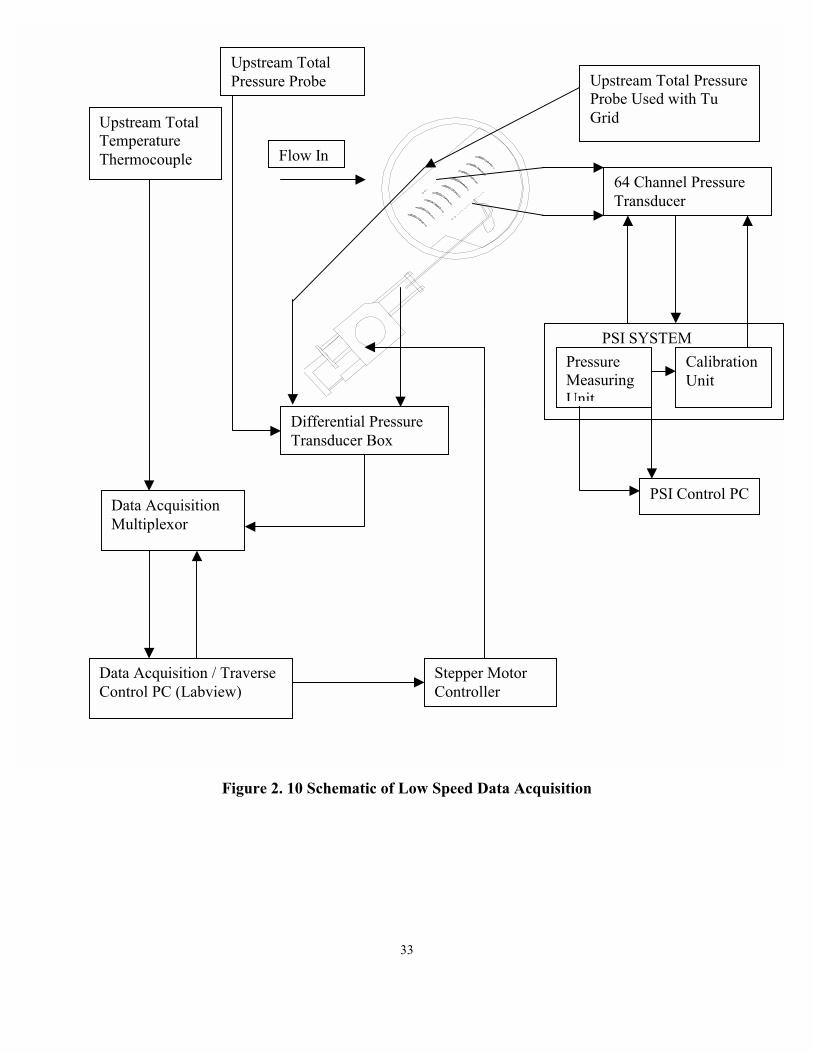
power supply of a constant +5 V DC. Figure 2.10 shows a schematic of the data acquisition
setup.
The voltage outputs from the pressure transducer box were recorded using Labview data
acquisition software. The Labview data acquisition system consisted of a personal computer and
multiplexor capable of recording 32 voltage signals and 32 thermocouple signals. The sampling
frequency and the number of samples to be recorded per channel were to be input by the
experimenter. For this experiment, data was sampled at 100 Hz and 1000 samples were recorded
per channel, which resulted in a 10 second sampling period. It should be noted that the Labview
Code is a low speed, steady-state measuring system and would not be suited for high-speed
measurements such as velocity fluctuations used in measurement of turbulence. The signals

32
acquired by Labview include: upstream total pressure, differential total pressure, traverse
position, and downstream static pressure from the traversing probe. After the PSI system
malfunction in the latter stages of this study upstream and downstream sidewall static pressure
was also recorded in Labview.
Two other signals were monitored during this testing but were not directly used in the
aerodynamic loss calculation. The relative humidity of the air entering the cascade was
monitored using a relative humidity sensor. In previous studies relative humidity higher than
10% have been found to increase the total loss level. In addition to humidity sensor, an
OMEGA type-K thermocouple was positioned approximately in the same location as the
upstream total pressure probe and monitored the total temperature entering the cascade. The
output from the thermocouple was recorded and converted to degrees Centigrade by the data
acquisition software. Although the total temperature measurement was not essential to the
aerodynamic loss calculation it was needed to reduce the turbulence intensity data generated by
the turbulence grid, and for the calculation of AVDR.
33
Figure 2. 10 Schematic of Low Speed Data Acquisi
PSI SYSTEM
Upstream Total Temperature Thermocouple
Data Acquisition Multiplexor
Data Acquisition / Traverse Control PC (Labview)
Upstream Total Pressure Probe
Differential Pressure Transducer Box
64 Channel Pressure Transducer
Calibration Unit
Stepper Motor Controller
Upstream Total Pressure Probe Used with Tu Grid
Pressure Measuring Unit
Flow In
tion
PSI Control PC
34
2.4.2 Hot Wire Setup and Measurements
The hot wire used for this work was a standard Dantec probe and was used for previous research
at Virginia Tech. The wire is positioned so that the two sets of two prongs are parallel at an
angle of 90o to its body (3.2mm stainless steel tubing). The dimension of the wire used was 5mm
(0.005 mm = 0.0002 inches), and were attached to the prongs using annealed Tungsten, either at
the manufacturer or at facilities at Virginia Tech. The hotwire was controlled using a Dantec
(55M01) anemometer equipped with a (55M10 CTA) standard bridge accessory. The standard
bridge was designed for use with a 5 meter BNC cable and was displayed in a window over the
cable compensation controls. A TSI Corp. IFA-100 anemometer was coupled with Dantec
anemometer for use of the IFA�s signal conditioner. IFA�s signal conditioner allowed the signal
to be filtered and offset as the flow condition dictates.
The frequency response of the hot wire was adjusted with two controls on the front panel of the
Dantec unit. The two controls are labeled �L� and �Q� which is more commonly known as cable
compensation. These controls are to be turned clockwise (CW) and counterclockwise (CCW)
until the proper test signal is seen on an oscilloscope, as documented in the manufacturer�s
literature. Over or under adjustment will cause the anemometer to become electronically
unstable. This tuning of the frequency response must be performed in a flow similar to the test
conditions such that the Reynold�s number (Re) of the wire is matched. In general, frequency
response increases with the adjustment of the cable compensation, but at an extreme tuning
position the system becomes instable. At no flow or low speed conditions a high frequency
response was very easily obtainable. However, since the frequency response is sensitive to
35
Reynold�s number, high Re flows cause greater instability and require a lower frequency
response, or in other words, a lower cable compensation. For this study the high Re flow
condition could not be obtained through bench testing. Therefore, the hotwire�s frequency
response was tuned inside of the test section of the wind tunnel. Since the run time of the tunnel
is approximately twenty seconds at steady-state conditions, this tuning required several
iterations.
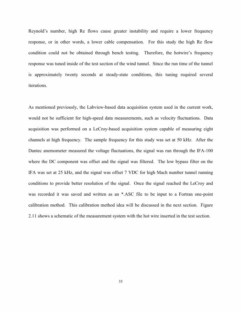
As mentioned previously, the Labview-based data acquisition system used in the current work,
would not be sufficient for high-speed data measurements, such as velocity fluctuations. Data
acquisition was performed on a LeCroy-based acquisition system capable of measuring eight
channels at high frequency. The sample frequency for this study was set at 50 kHz. After the
Dantec anemometer measured the voltage fluctuations, the signal was run through the IFA-100
where the DC component was offset and the signal was filtered. The low bypass filter on the
IFA was set at 25 kHz, and the signal was offset 7 VDC for high Mach number tunnel running
conditions to provide better resolution of the signal. Once the signal reached the LeCroy and
was recorded it was saved and written as an *.ASC file to be input to a Fortran one-point
calibration method. This calibration method idea will be discussed in the next section. Figure
2.11 shows a schematic of the measurement system with the hot wire inserted in the test section.
36
Figure 2. 11 Schematic of High Speed Data Acquisition with Hot Wire
Upstream Total Temperature Thermocouple
Upstream Total Pressure Probe
Data Acquisition Multiplexor
Data Acquisition / Traverse Control PC (Labview)
Differential Pressure Transducer Box
Hotwire
Dantec Anemometer
IFA-100 Filter and Offset
LeCroy High Speed Data Acquisition
LeCroy Data Acquisition Control PC
Upstream Total Pressure Probe Used with Tu Grid

37
2.4.3 Static Pressure Measurements on the Blade Surface
Static pressure taps were fabricated on both the pressure and suction surfaces of the compressor
stators. A photograph of the instrumented stators is shown in Figure 2.12. The static pressure
holes were positioned at approximately 4% chord apart, and measure from about 4% chord to
approximately 90% chord. Stainless steel tubing 1/16 inch in diameter, was placed into the
machined slots using aerospace structural epoxy and then sanded so that the geometry of the
stator was unchanged. After assembling the instrumented blades into the Plexiglas side walls,
they were checked for leaks using Snoop leak detector. Since each blade is instrumented with 18
static pressure holes, the leakages of one or two taps was not catastrophic to the experiment and
therefore, were abandoned. Each static pressure was measured with an individual differential
pressure transducer and recorded with the low speed data acquisition system. The range of these
measuring transducers was from +/-5psig to +/-15psig.
Figure 2. 12 Instrumented Static Pressure Stators
38
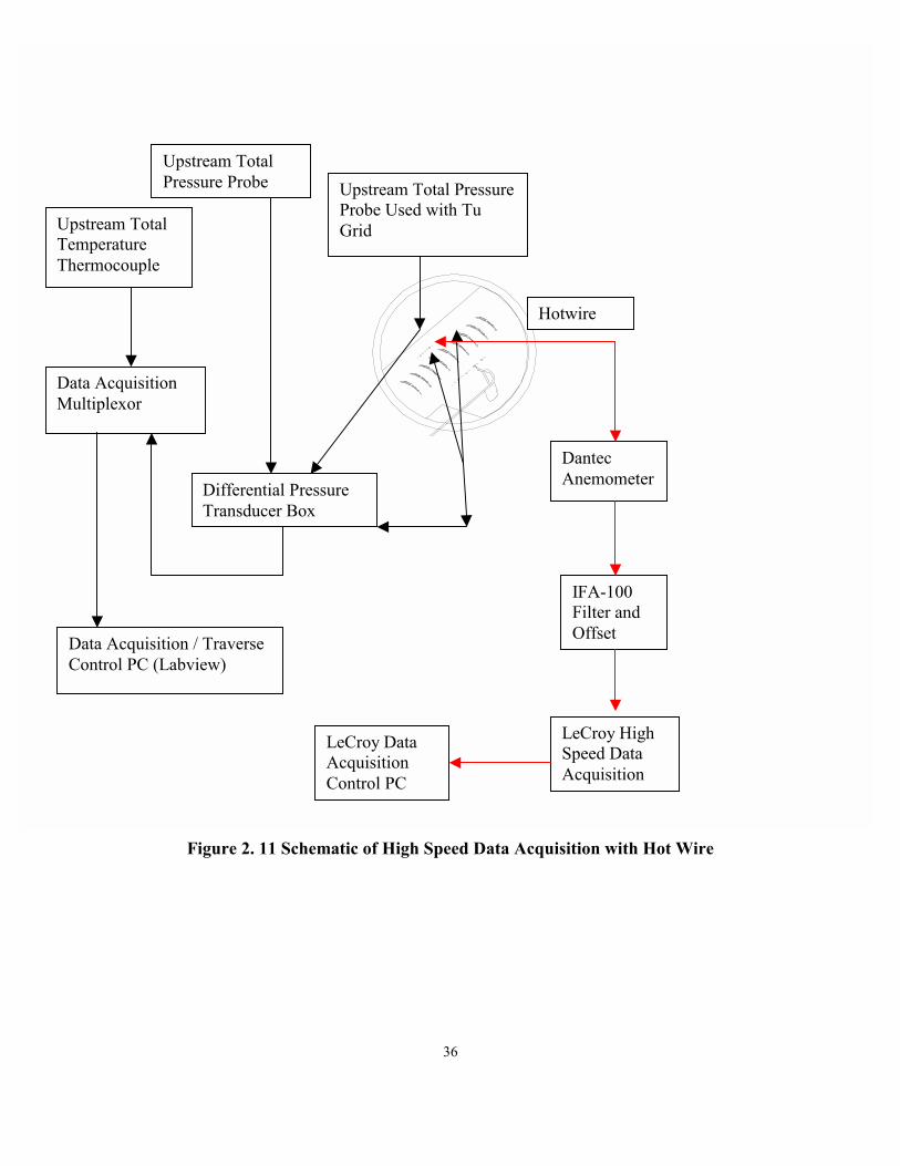
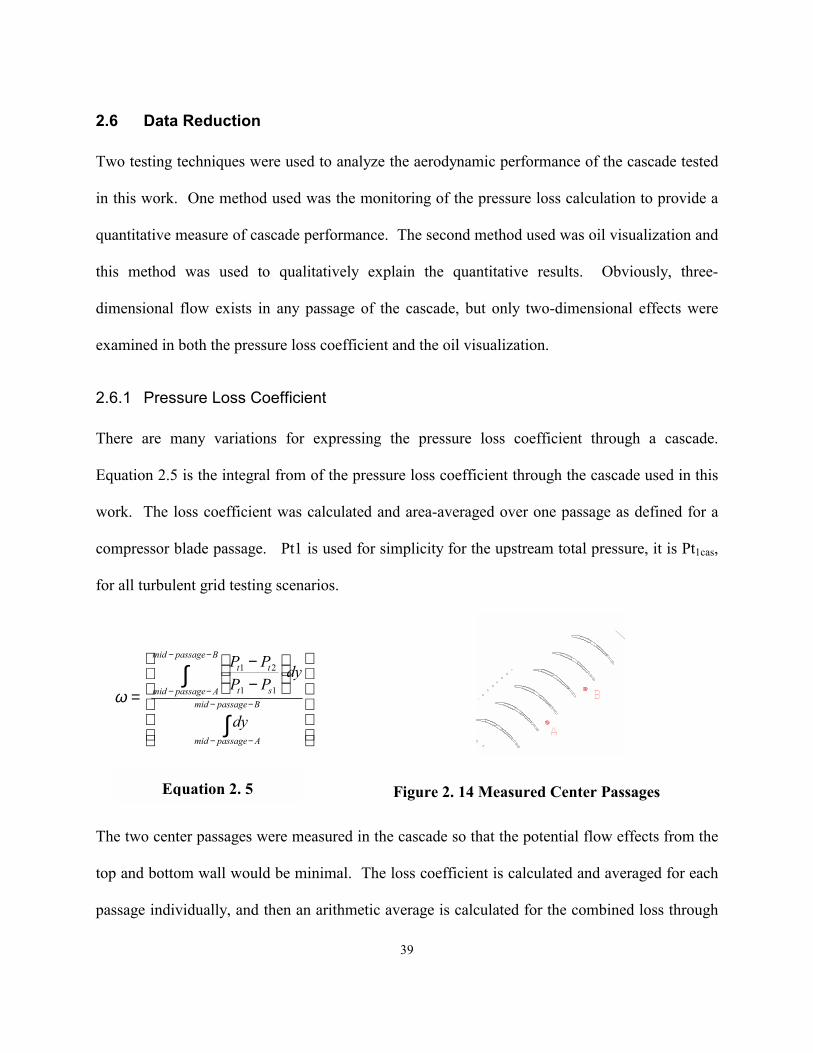
2.5 Oil Flow Visualization
An efficient technique for gaining a physical picture of the flow pattern for qualitative analysis is
the use of surface oil flow visualization. Surface oil visualization involves coating the blade
surfaces and Plexiglas sidewalls with contrasting fluorescent colored paint. The paint is made up
of a mixture of oil and dye, and is mixed at 3:1 oil to dye. After the painted cascade is
assembled it is inserted into the test section and the tunnel is run at a know pressure and Mach
number. The pattern of oil formed by the mass flow through the test section on the blade surface
and sidewall is used to qualitatively analyze the cascade flow field. Even though this pattern can
be easily seen under normal light, a fluorescent light is used when taking still photographs to
make the pattern even more distinguishable. The oil visualization is very helpful to examine the
effects of flow separation, probable shock location, and secondary flow. The qualitative
analysis of these flow phenomena makes the measured aerodynamic properties easier to explain
and understand. Figure 2.13, provides an example of this technique in a picture of the entire
cascade, however, more detailed pictures will be included in the next chapter of this work.
Figure 2. 13 Oil Visualization Entire Cascade
2.6 Data Reduction
Two testing techniques were used to analyze the aerodynamic performance of the cascade tested
in this work. One method used was the monitoring of the pressure loss calculation to provide a
quantitative measure of cascade performance. The second method used was oil visualization and
this method was used to qualitatively explain the quantitative results. Obviously, three-
dimensional flow exists in any passage of the cascade, but only two-dimensional effects were
examined in both the pressure loss coefficient and the oil visualization.
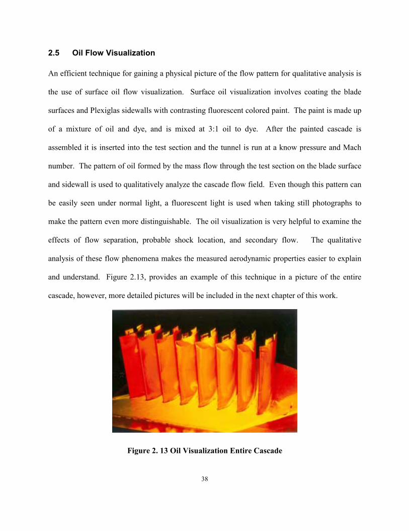
2.6.1 Pressure Loss Coefficient
There are many variations for expressing the pressure loss coefficient through a cascade.
Equation 2.5 is the integral from of the pressure loss coefficient through the cascade used in this
work. The loss coefficient was calculated and area-averaged over one passage as defined for a
compressor blade passage. Pt1 is used for simplicity for the upstream total pressure, it is Pt1cas,
for all turbulent grid testing scenarios.
Figure 2. 14 Measured Center Passages
The two ce
top and bo
passage ind
−−
=
∫
∫−−
−−
−−
−−Bpassagemid
Apassagemid
Bpassagemid
Apassagemid st
tt
dy
dyPPPP
11
21
ω
E
quation 2. 539
nter passages were measured in the cascade so that the potential flow effects from the
ttom wall would be minimal. The loss coefficient is calculated and averaged for each
ividually, and then an arithmetic average is calculated for the combined loss through

40
both passages. This is done because the flow in both passages is not exactly identical and this
slight difference is recorded and averaged. The static pressure measurements taken upstream of
the leading edge of the stators to be examined were time averaged over the ten second data
acquisition window and in the steady-state portion of the running of the wind tunnel. The static
pressure readings have an insignificant fluctuation over this time, therefore, making this average
acceptable. The downstream total pressure is measured over the two passages to be examined
and therefore is dependent upon pitch-wise location. The total pressure difference between state
1 (upstream) and state 2 (downstream) is calculated at the respective instantaneous time and
position of the downstream traverse. The upstream total pressure measurement was made at
single location because the upstream flow was found to be uniform during the upstream traverse
testing mentioned previously and is also time averaged.
Once the upstream static and total pressure measurements are time-averaged the inlet Mach
number is calculated using the following equation:
The local exit Mach number is calculated in the same manner using the following substitution of
states:
This exit Mach number is dependent on the pitch-wise location of the downstream traverse. This
measurement was very convenient due to the three-hole traversing probe that had the capability
to measure both total and static pressure at the same point. g=1.4 was used for all calculations.
121
1
1 )2
11( −⋅−+= γγ
γ MPP
s
t Equation 2.6
122
2
2 )2
11( −⋅−+= γγ
γ MPP
s
t Equation 2. 7

41
From the measured upstream total temperature and the calculated inlet Mach number the
upstream static temperature can now be calculated from the following equation:
Now with the upstream static temperature, the density can be calculate
as:
Hence, the inlet velocity can be determined using the speed of sound rela
This velocity is based on free-stream measurements and is no indication
the inlet of the cascade. The Axial Velocity Density Ratio (AVDR)
cascade using the following equation:
The AVDR is a measure of the two-dimensionality of the flow through
indication of the flow turning through the passage between two bla
coefficient is often found to be inversely proportional to the calculated A
)2
11( 21
1
1 MTT
s
t ⋅−+= γ
1
1
s
s
TRP⋅
=ρ
1
11
sTRMU⋅⋅
=γ
( )
( )
⋅
⋅=
∫
∫−−
−−
−−
−−Bpassagemid
ApassagemidA
Bpassagemid
ApassagemidMSA
dyU
dyUAVDR
11
22
ρ
ρ
Equation 2.8
d from the ideal gas law
t
o
th
d
V
Equation 2.9
ion in Equation 2.10.
Equation 2.10f the velocity profile to
was calculated for this
Equation 2.11
e cascade. It is also an
es. The pressure loss
DR for a cascade.

42
51.0
17.0
Re48.0 ⋅=
⋅
−
TsTmNu
msmmsw kTTV
kTTVNu
⋅−∝
⋅−∝
)()(
22
2.6.2 One-Calibration and Turbulence Intensity
The one-point calibration theory was taken and developed from Homberg (1996) and its details
will be included in the appendix of this work. The basis of this calibration is the following
equation:
where (Tm/Ts) is a temperature correction factor, and the R
than 44. The restriction on the Re number is because Re =
turbulent transition for flow over the wire occurs (Holmberg,
eloquent detail of the validity of the assumptions in using E
calibration. Putting each piece of Equation 2.12 into known m
that can be used for calibration yields the following equation:
where
where, V is the hot wire(HW) voltage and the tunnel st
variables. All manufacturer given wire properties should sta
of a constant temperature anemometer. So if constant wire te
constant resistances should also be maintained (Holmberg,19
equation reduces to: since (Tw - Ts) =
,m
kdhNu ⋅=
()(
)(
)()()( 2
1
2
www
w
w
TTLd
RRRV
Tareapowerh
−⋅⋅⋅
+⋅
=∆⋅
=π
Equation 2.12 (Holmberg, 1996)
eynolds number has to be greater
44 is the point where laminar to
1996). Holmberg (1996) goes into
quation 2.12 for one point hotwire
easured quantities, and into a form
atic tem
y const
mperat
96). Th
2(Tm
)s
Equation 2.13 (Holmberg,1996)
perature Ts, are the only
ant in theory, due to the use
ure (Tw), is maintained then
erefore the Nusselt number
� Ts)
Equation 2.14 (Holmberg,1996)

17.0251.0
)(
−
⋅
⋅−⋅=
⋅
TsTm
kTTVCU
msmm
m
µρ
4103724 103327.5102694.5108556.222371.08.1037 ssssair TxTxTxTCp ⋅−⋅+⋅+⋅−= −−−
Now, substituting Equation 2.14 into Equation 2.12, taking the constant wire diameter out of Re,
transposing left and right sides for convenience, and inserting a calibration constant yields:
Simplified to:
Equation 2.16 was used for the calibration of the HW for all turbulence grid measurements. The
general step-by-step procedure for applying these equations is as follows (Holmberg,1996).
Find the average Pt, Tt, and V (HW voltage) over the selected HW sample.
Solve for Ts, using the isentropic relationship with the known inlet Mach number and g = 1.4 as
the initial value.
Calculate what your new Cpair based on the following variable specific heat equation:
Proceed now to calculate a
constant C. These values a
Equation 2.15 (Holmberg,1996).
'Re' NuC ⋅= Equation 2.16 (Holmberg,1996).
E
⋅Ks
m2
2
quation 2.17 (Holmberg, 1996).
43
new g, Ps, Ts, U, Tm, rm, mm, km, Re�, Nu�, and finally the calibration
re found using basic compressible flow and heat transfer equations.

44
This calculated constant C is for the HW used, and will remain constant from run to run, with
some small drift over time. This constant can then be used for the conversion of all the HW
bridge voltage data acquired in that run to a velocity series. It should be noted that this
documented procedure is an abridged version and that a detailed procedure is documented in
Holmerg�s (1996) dissertation attached in the appendix of this work.
When using the above calibration to solve for the velocity, the values of Re� and Nu� must be
solved iteratively with the help of a small FORTRAN code (Holmberg,1996). The code used in
this work is Fortran Powerstation and will be included in the appendix. The progression is
similar to above calibration equations, but the result is U for each sampled data point instead of a
calibration constant (Holmberg, 1996). The following procedure leads to the instantaneous
velocities:
Solve for Cp, Ts, Tm, km, m, g, as above.
Solve for Mach number, M.
The Ps = f(Pt, g, M).
Solve for Nu� using the instantaneous HW voltage.
51.01
)'()( NuCU ⋅⋅=⋅ µρ , where Re� = C*Nu�
Mean density from the low speed data, Ps,m/R*Ts
Then instantaneous U= (r *U)/rm if density fluctuations are assumed negligible.
Iterate the above sequence until U converges to a solution.
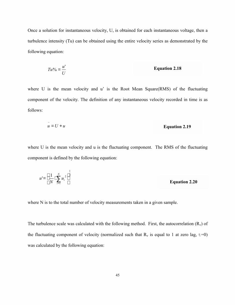
45
Once a solution for instantaneous velocity, U, is obtained for each instantaneous voltage, then a
turbulence intensity (Tu) can be obtained using the entire velocity series as demonstrated by the
following equation:
where U is the mean velocity and u� is the Root Mean Squa
component of the velocity. The definition of any instantaneous ve
follows:
where U is the mean velocity and u is the fluctuating component.
component is defined by the following equation:
where N is to the total number of velocity measurements taken in a
The turbulence scale was calculated with the following method. Fir
the fluctuating component of velocity (normalized such that Rv is
was calculated by the following equation:
UuTu '% =
uUu +=~
21
1
21'
⋅= ∑
=
N
iiu
Nu
Equation 2.18
re(RMS) of the fluctuating
locity recorded in time is as
The
given
st, th
equ
Equation 2.19
RMS of the fluctuating
sa
e a
al
Equation 2.20mple.
utocorrelation (Rv) of
to 1 at zero lag, t=0)
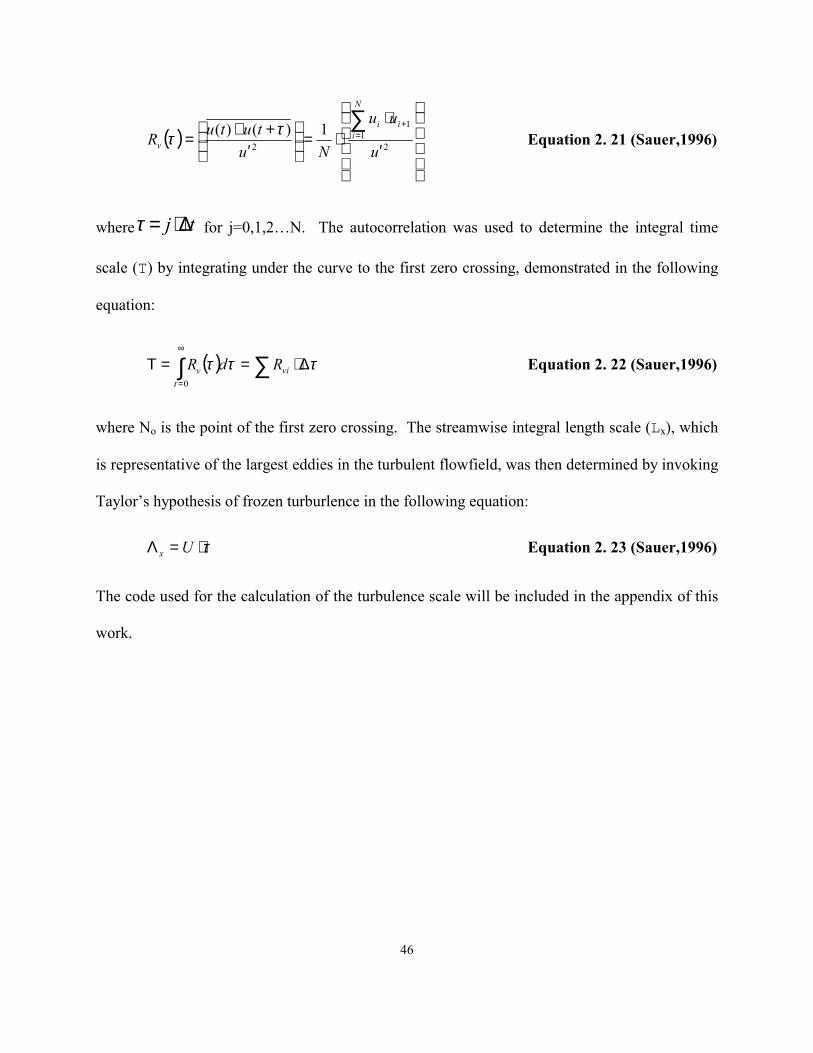
46
( )
′
⋅⋅=
′+∗=
∑=
+
21
1
2
1)()(u
uu
NututuR
N
iii
vττ Equation 2. 21 (Sauer,1996)
where tj ∆⋅=τ for j=0,1,2�N. The autocorrelation was used to determine the integral time
scale (T) by integrating under the curve to the first zero crossing, demonstrated in the following
equation:
( ) ∑∫ ∆⋅==Τ∞
=
τττ vit
v RdR0
Equation 2. 22 (Sauer,1996)
where No is the point of the first zero crossing. The streamwise integral length scale (Lx), which
is representative of the largest eddies in the turbulent flowfield, was then determined by invoking
Taylor�s hypothesis of frozen turburlence in the following equation:
τ⋅=Λ Ux Equation 2. 23 (Sauer,1996)
The code used for the calculation of the turbulence scale will be included in the appendix of this
work.

47
Chapter 3 EXPERIMENTAL RESULTS AND DISCUSSION
This chapter will review and discuss the results obtained from cascade experiments with and
without increased free-stream turbulence at varying cascade angles and inlet Mach numbers.
Section 3.1 discusses the turbulence level results obtained from the hotwire measurements, while
section 3.2 will display and discuss the aerodynamic performance data recorded for the varying
experimental scenarios. At the end of each of the respective sections, work from previous
researchers will be compared to the current work to try to explain and validate the recorded data
and observable trends found in the results from the current experiment. It should be noted for all
data presented in this chapter that incidence angle is denoted as �cascade angle�. The angle is
referenced to in this manner due to the uncertainty of actual inlet flow angle to the cascade. It is
believed from preliminary testing that the inlet flow may be inclined up to 1.5o. It should also be
mentioned that the AVDR displayed on the loss coefficient figures is given in a range due to the
lack of necessary means to control the AVDR to a constant value.
3.1 Turbulence Level Measurements
Only one passive turbulence grid was used in this experiment, so therefore, the turbulence level
generated from this grid was used for all turbulence testing and was compared to the baseline
case of no grid generated turbulence. The Reynolds number range of all testing conditions was
about 1-2x10⁶. The baseline turbulence level was measured to be approximately 0.1-0.2%, at all
Reynolds� numbers tested. The turbulence level was approximately 1.6% at the lower extreme
of the Reynolds� number range, and approximately 1.3% at the higher extreme. The fluctuating
velocity plots versus time, are displayed in Figure 3.1 for all of the respective experimental
cases.

48
Figure 3. 1 HW Voltage Plots for Respective Tu Intensities
Fluctuating Velocity vs TimeNo Grid;Re~1.2x10⁶ ;Tu~0.15%
-15
-10
-5
0
5
10
15
0 0.5 1 1.5 2 2.5 3
time (ms)
Velo
city
(m/s
)
Fluctuating Velocity vs TimeWith Tu;Re~2x10⁶ ;Tu~1.35%
-15
-10
-5
0
5
10
15
0 0.5 1 1.5 2 2.5 3
time (ms)
Vel
ocity
(m/s
)
Fluctuating Velocity vs TimeWith Tu;Re~1.2x10⁶ ;Tu~1.64%
-15
-10
-5
0
5
10
15
0 0.5 1 1.5 2 2.5 3
time (ms)
Vel
ocity
(m/s
)
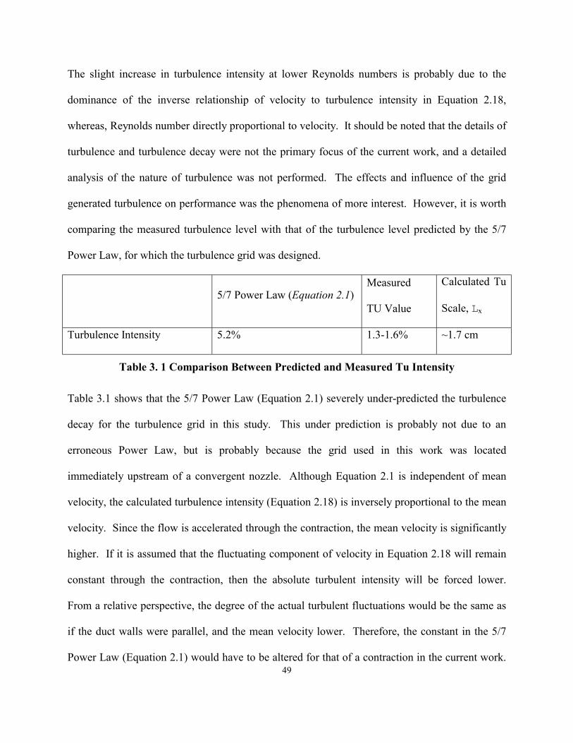
49
The slight increase in turbulence intensity at lower Reynolds numbers is probably due to the
dominance of the inverse relationship of velocity to turbulence intensity in Equation 2.18,
whereas, Reynolds number directly proportional to velocity. It should be noted that the details of
turbulence and turbulence decay were not the primary focus of the current work, and a detailed
analysis of the nature of turbulence was not performed. The effects and influence of the grid
generated turbulence on performance was the phenomena of more interest. However, it is worth
comparing the measured turbulence level with that of the turbulence level predicted by the 5/7
Power Law, for which the turbulence grid was designed.
5/7 Power Law (Equation 2.1)
Measured
TU Value
Calculated Tu
Scale, Lx
Turbulence Intensity 5.2% 1.3-1.6% ~1.7 cm
Table 3. 1 Comparison Between Predicted and Measured Tu Intensity
Table 3.1 shows that the 5/7 Power Law (Equation 2.1) severely under-predicted the turbulence
decay for the turbulence grid in this study. This under prediction is probably not due to an
erroneous Power Law, but is probably because the grid used in this work was located
immediately upstream of a convergent nozzle. Although Equation 2.1 is independent of mean
velocity, the calculated turbulence intensity (Equation 2.18) is inversely proportional to the mean
velocity. Since the flow is accelerated through the contraction, the mean velocity is significantly
higher. If it is assumed that the fluctuating component of velocity in Equation 2.18 will remain
constant through the contraction, then the absolute turbulent intensity will be forced lower.
From a relative perspective, the degree of the actual turbulent fluctuations would be the same as
if the duct walls were parallel, and the mean velocity lower. Therefore, the constant in the 5/7
Power Law (Equation 2.1) would have to be altered for that of a contraction in the current work.

50
Table 3.1 also shows the calculated integral turbulence scale for this work, which stayed very
close to constant since the grid was only located in one position with only one diameter of bars.
Since the nature of turbulence is beyond the scope of this work, little previous research was
examined in order to validate any speculation on the effects of the contraction or the scale.
However, Kiock(1972) had documented the inverse relationship between Reynolds number and
turbulent intensity. During his experiments on a six-stage axial compressor, Kiock found that
when Reynolds numbers where on the order of 2x10⁵, that turbulence intensity was found to be
only 3%. When operating his experiment at a Reynolds number of 0.6x10⁵, Kiock found that the
turbulence intensity had increased to 5%. Since the current testing covers a smaller range of
Reynolds number, the small variance in turbulence intensity is feasible.
3.2 Aerodynamic Data Regarding Performance and the Boundary Layer
3.2.1 Total Pressure Loss Coefficient
The behavior of the total pressure loss coefficient was the parameter of primary focus in the
current work. The pressure loss coefficient will be displayed in the following figures versus
cascade angle for a given inlet Mach number. A summary will also be given for the pressure
loss coefficient versus inlet Mach number to show the trend of performance as a function of a
different parameter. The following figures will include the trend for both baseline and generated
turbulence running conditions. The pressure loss coefficient is based on area averaged
downstream total pressure traverse of the center two passages in the cascade. The loss
coefficient was interpolated when necessary to fit the plot format in the following figures.

51
Figure 3. 2 Loss Coefficient vs. Incidence for Inlet Mach Numbers 0.60, 0.65, 0.70, 0.75
T otal P r es s u r e L os s Coefficien t vs In let Cas cade An gle
OR G B lade; AVD R =0.96~1 .12
0
0 .0 5
0 .1
0 .1 5
0 .2
0 .2 5
0 .3
0 .3 5
3 6 .4 3 8 .4 4 0 .4 4 2 .4 4 4 .4 4 6 .4 4 8 .4 5 0 .4
Cas cade An gle (degr ees )
ω
M1 =0 .6 5 , wi th T u. Grid
M1 =0 .6 5 , wi thout T u. Grid
T otal P r es s u r e L os s Coeff icien t v s In let Cas cade An gle
OR G B lade; AVD R =0 .96~1 .12
0
0 .0 5
0 .1
0 .1 5
0 .2
0 .2 5
0 .3
0 .3 5
3 6 .4 3 8 .4 4 0 .4 4 2 .4 4 4 .4 4 6 .4 4 8 .4 5 0 .4
Cas cade An gle (degr ees )
ω
M 1 =0 .7 5 , wi th T u. Gr id
M 1 =0 .7 5 , wi thout T u. Gr id
T otal P r es s u r e L os s Coefficien t vs In let Cas cade An gle
OR G B lade; AVD R =0.96~1.12
0
0 .0 5
0 .1
0 .1 5
0 .2
0 .2 5
0 .3
0 .3 5
3 6 .4 3 8 .4 4 0 .4 4 2 .4 4 4 .4 4 6 .4 4 8 .4 5 0 .4
Cas cade An gle (degr ees )
ω
M1 =0 .6 0 , wi th T u. Grid
M1 =0 .6 0 , wi thout T u. Grid
T otal P r es s u r e L os s Coefficien t vs In let Cas cade An gle
OR G B lade; AVD R =0.96~1.12
0
0 .0 5
0 .1
0 .1 5
0 .2
0 .2 5
0 .3
0 .3 5
3 6 .4 3 8 .4 4 0 .4 4 2 .4 4 4 .4 4 6 .4 4 8 .4 5 0 .4Cas cade An gle (degr ees )
ω
M 1 = 0 .7 0 , wi th T u. Gr id
M 1 = 0 .7 0 , wi thout T u. Gr i d
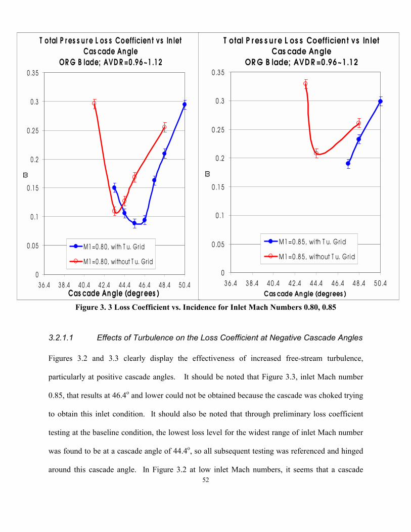
52
Figure 3. 3 Loss Coefficient vs. Incidence for Inlet Mach Numbers 0.80, 0.85
3.2.1.1 Effects of Turbulence on the Loss Coefficient at Negative Cascade Angles
Figures 3.2 and 3.3 clearly display the effectiveness of increased free-stream turbulence,
particularly at positive cascade angles. It should be noted that Figure 3.3, inlet Mach number
0.85, that results at 46.4o and lower could not be obtained because the cascade was choked trying
to obtain this inlet condition. It should also be noted that through preliminary loss coefficient
testing at the baseline condition, the lowest loss level for the widest range of inlet Mach number
was found to be at a cascade angle of 44.4o, so all subsequent testing was referenced and hinged
around this cascade angle. In Figure 3.2 at low inlet Mach numbers, it seems that a cascade
T o tal P r es s u r e L os s Coeff icien t vs In let Cas cade An gle
OR G B lade; AVD R =0.96 ~1 .1 2
0
0 .0 5
0 .1
0 .1 5
0 .2
0 .2 5
0 .3
0 .3 5
3 6 .4 3 8 .4 4 0 .4 4 2 .4 4 4 .4 4 6 .4 4 8 .4 5 0 .4Cas cade An gle (degr ees )
ω
M1 =0 .8 0 , wi th T u. Gr id
M1 =0 .8 0 , wi thout T u. Gr id
T otal P r es s u r e L os s Coeff icien t vs In let Cas cade An gle
OR G B lade; AVD R =0.96~1.12
0
0 .0 5
0 .1
0 .1 5
0 .2
0 .2 5
0 .3
0 .3 5
3 6 .4 3 8 .4 4 0 .4 4 2 .4 4 4 .4 4 6 .4 4 8 .4 5 0 .4Cas cade An gle (degrees )
ω
M1 =0 .8 5 , wi th T u. Gr id
M1 =0 .8 5 , wi thout T u. Gr id

53
angle of 43.4o, is a critical cascade angle where the effect of free-stream turbulence on the loss
coefficient starts to become negligible for remaining negative cascade angles. This negligible
effect of turbulence at intermediate to low Mach numbers, and negative incidence, may best be
explained by the possibility that the flow is not separated from the blade surface at either the
baseline condition or with generated turbulence. Therefore, even if the transition point is moved
by the free stream turbulence, any reduction in losses due to delayed separation cannot be
realized. It should be noted that no oil visualization was done at cascade angles below 44.4o ,
and limited visualization was done at 44.4o due to time restrictions. Therefore, the above
speculation cannot be effectively supported. This condition of nonseparated flow may best be
represented in Figure 3.4.
Figure 3. 4 Oil Visualization, I=44.4o, M1~0.65
SS
LE TE

54
Figure 3.4 is a picture of the suction side of a stator located in the center passage of the cascade.
This stator was tested at a cascade angle of 44.4o and an inlet Mach number of approximately
0.65, with generated free-stream turbulence. It appears from Figure 3.4 that flow at the mid-span
of the blade is attached over the full suction surface. Since Figure 3.2 shows some reduction in
losses for this cascade angle and inlet Mach number, the baseline testing condition probably has
some small turbulent separation near the trailing edge of the stator. Whereas, with generated
turbulence, turbulent separation appears to have been totally eliminated at mid-span. It should be
noted that the suction surface of the blade was painted from 0-50% chord(pink), and the pressure
side painted from 50-100% chord(yellow) in order to try to ascertain flow direction. From
Figure 3.4, it may be reasonable to assume that at negative cascade angles the trend of
completely attached flow is developing. This leads to the negligible differences in the loss
coefficient with and without generated turbulence at negative cascade angles.
At an inlet Mach number of 0.75 in Figure 3.2 and an inlet Mach number of 0.80 in Figure 3.3,
the effect of free stream turbulence at negative cascade angles, is seen to be that of an adverse
one. Since no visualization or blade surface static pressure measurements were conducted at
these cascade angles, the author can only speculate based on Figure 3.3 that the increased
turbulence may have caused a higher degree of separation. This may be because these cascade
angles and inlet Mach numbers are approaching the stalling point of the cascade.

55
3.2.1.1 Effects of Turbulence on the Loss Coefficient at Positive Cascade Angles
From Figures 3.2 and 3.3, the cascade angle range of 44.4-48.4o, a substantial loss-reduction is
realized for all inlet Mach numbers tested. It may now be helpful to the reader�s perspective to
re-plot the loss coefficient versus inlet Mach number for the two extremes of the incident angle
range previously mentioned.
Figure 3. 5 Loss vs M1; I=44.4o Figure 3. 6 Loss vs M1; I=48.4o
T otal P r es s u r e L os s vs In let M ach Nu mber
OR G B lade; AVD R =0 .96~1 .12
0
0 .1
0 .2
0 .3
0 .4
0 .5 0 .6 0 .7 0 .8 0 .9
In let M ach Nu mber
ω
4 4 .4 degs , w/o T u
4 4 .4 degs , wi th T u
T otal P r es s u r e L os s vs In let M ach Nu mber
OR G B lade; AVD R =0 .96~1 .12
0
0 .1
0 .2
0 .3
0 .4
0 .5 0 .6 0 .7 0 .8 0 .9In let M ach Nu mber
ω4 8 .4 degs , wi th T u
4 8 .4 degs , wi thout T u

56
Figures 3.5 and 3.6, may make it more visually apparent to the effects of increasing free-stream
turbulence on cascade performance. Table 3.2 is a summary of the percentage loss reduction for
Figures 3.2, 3.3, 3.5, and 3.6 at positive cascade angles.
M1 44.4o 45.4o 46.4o 47.4o 48.4o Cascade Angle
0.6 42% 56% 44% 26% 13% Loss Reduction
0.65 37% 55% 42% 24% 11%
0.7 35% 54% 46% 23% 17%
0.75 34% 56% 54% 31% 20%
0.8 17% 50% 52% 28% 18%
0.85 NA NA NA 22% 11%
Table 3. 2 Summary of Loss Reduction
Table 3.2 shows a summary of the loss reduction due to effects of increased free-stream
turbulence at the experimental �hinge� point through four degrees of positive cascade incidence.
In general, the loss reduction shown in Table 3.2 is probably due to the delay in turbulent
separation on the blade suction surface. This delay may best be explained by the suppression of
the laminar separation bubble with increasing free-stream turbulence. With this suppression, the
turbulent portion of the boundary layer will cover more of the blade�s surface, making the
boundary layer more tolerant to the adverse pressure gradient over the airfoil. The first
noticeable trend in Table 3.2, with the exception 45.4o, is that with increasing cascade incidence
the effectiveness of generated turbulence on losses is dramatically reduced at a given inlet Mach
number. In general, this trend may best be explained by the probability that the location of
transition and turbulent separation generally propagate toward the leading edge of the blade with

57
increasing incidence. With the addition of generated free-stream turbulence, the extent of the
forward propagated transition may be further suppressed, allowing the separation of the turbulent
boundary layer to be delayed. Even with increasing inlet Mach number, the cascade angle of
45.4o, appears to be an optimum cascade angle where turbulence is most effective (Table 3.2).
The trend developed with increasing inlet Mach number is one that points to an optimum Mach
number of 0.75. At this Mach number, the effect of turbulence on losses seems to be most
effective for cascade angles higher than 44.4o. At 44.4o and inlet Mach numbers above 0.75, the
loss reduction is found to decrease. This may be because the cascade is approaching or even
reaches the point of complete separation on the suction surface of the stators in the cascade. This
condition is different for every cascade angle and occurs at different inlet Mach numbers for
each of these cascade angles, respectively. When the cascade reaches this condition, the effect of
turbulence seems to be a secondary effect to that of a shock wave that could exist in the blade
passage. Therefore, the strength of this shock and its interaction with the boundary layer is
believed to determine the effectiveness of the generated free stream turbulence on losses at this
condition. This topic will be discussed further in the section 3.2.2, where the results from the
imbedded static pressure taps in the blade surfaces are presented.
It is now necessary to compare the loss results and trends of the current work with that of
previous research. It will be helpful to first compare the loss level of the current work at baseline
conditions (No Grid) with the research of Carter (2001), which was performed in the same
laboratory and test section of the current work. Carter�s research at his baseline condition was
performed on stators that had a 4-inch chord, 6-inch span, 2.22 solidity ratio, and a total turning
angle of 69o (47o-current work). The design inlet Mach number in Carter�s testing was

58
approximately 0.8 and a blade chord Reynolds number of approximately 2x10⁶. Carter�s results
will be compared to Figure 3.3 at an inlet Mach of 0.80. Carter�s design cascade angle will be
compared to the lowest loss level cascade angle (44.4o), of the current work.
Total Pressure Loss Coefficient vs Inlet Cascade Angle
ORG Blade; AVDR=0.96~1.12
0
0.05
0.1
0.15
0.2
0.25
0.3
0.35
36.4 38.4 40.4 42.4 44.4 46.4 48.4 50.4Cascade Angle (degrees)
ω
M1=0.80, without Tu. Grid
Carter(2001)
Figure 3. 7 Loss Level Comparison (Carter, 2001)
Figure 3.7 shows a loss level comparison of both the high turning stators of the current work,
with that of the even higher turning stators of Carter (2001). The inlet Mach number is 0.80 for
both cases displayed in Figure 3.7. It should be reiterated that the lowest loss level for the widest
range of inlet Mach number was at a cascade angle of 44.4o, in the current work, and therefore
was used as an �experimental hinge angle� for all-further testing. The loss level at the design
cascade angle of Carter�s work compares very favorably for that of the current work, while the
Current Work Lowest Loss Level Cascade Angle of 44.4o
Carter(2001) Design Cascade Angle

59
off-design angles are quite different. From Figure 3.7, the current work has documented losses
below that of Carter�s work at a cascade angle of 43.4o. However at angles outside of this 2o
range, Carter�s stators are far more superior to the stators in the current work. The stators of the
current work are depicted in Figure 3.7 to be more sensitive to changes of the cascade angle, in
which the extent of the laminar separation bubble on the blade surface plays a major role.
In order to provide insight to the effect of increasing free-stream turbulence on the loss
coefficient, the work of Evans (1985) was examined. Evans conducted experiments on a
compressor cascade stator that had a chord length of 1 foot, and total turning of 43.65o. At all
testing conditions Evans documents that the Reynolds number based on chord was 5x10⁵.
Figure 3. 8 Effect of Tu on Losses and Deviation Angle (Evans,1985)
Figure 3.8 is a summary of the loss and deviation angle reduction that Evans observed with
increasing turbulence intensities. Note that he documents a slight increase the loss coefficient at
turbulent intensities up to 3%. He credits this behavior to the fact that at lower turbulent
intensities the boundary layer displays a thickening behavior. These phenomena will be

60
discussed further in the next section where the isentropic Mach number distribution will be
presented and discussed. At intensities of 3% and higher he notes a decrease in losses. In
comparison with the results of the current work, loss reduction was seen at turbulent intensities
as little as 1.6%. It is possible that a unique loss reduction curve, as seen in Figure 3.8, exists
for different stators, which also may have a different �hypothetical� turbulent intensity where the
loss coefficient starts to be reduced. Therefore, only the evidence of the tendency of increased
turbulent free-streams as a mechanism to reduce the loss coefficient is relative to this work. It is
unknown how a Reynolds number as high as the current work would affect the loss trend in
Figure 3.8. Evans further supports his reduction in losses with a measurement of the deviation
angle near the trailing edge of the stator. He documents that at all turbulent intensities tested that
the deviation angle decreases. In the current work the deviation angle was not measured, but
from Figure 3.8, it is reasonable to assume that the deviation angle also decreased with the
increasing turbulent free-stream.
The work of Citavy (1977) was also examined in order to gain additional information on the
effects of increased free stream turbulence on the loss coefficient of a compressor cascade.
Citavy conducted experiments on prescribed velocity distribution (PVD) airfoils at a Reynolds
number range of 0.6-2x10⁵, and a range of turbulence intensities of 0.35%-4.4%. The PVD had
a chord of 140 mm. Again, due to the low Reynolds number range the results are limited in a
quantitative sense, but the trend of the results are reasonable for qualitative comparison.
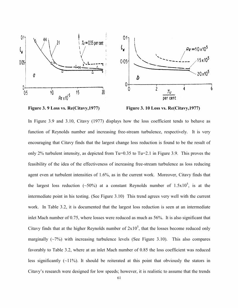
61
Figure 3. 9 Loss vs. Re(Citavy,1977) Figure 3. 10 Loss vs. Re(Citavy,1977)
In Figure 3.9 and 3.10, Citavy (1977) displays how the loss coefficient tends to behave as
function of Reynolds number and increasing free-stream turbulence, respectively. It is very
encouraging that Citavy finds that the largest change loss reduction is found to be the result of
only 2% turbulent intensity, as depicted from Tu=0.35 to Tu=2.1 in Figure 3.9. This proves the
feasibility of the idea of the effectiveness of increasing free-stream turbulence as loss reducing
agent even at turbulent intensities of 1.6%, as in the current work. Moreover, Citavy finds that
the largest loss reduction (~50%) at a constant Reynolds number of 1.5x10⁵, is at the
intermediate point in his testing. (See Figure 3.10) This trend agrees very well with the current
work. In Table 3.2, it is documented that the largest loss reduction is seen at an intermediate
inlet Mach number of 0.75, where losses were reduced as much as 56%. It is also significant that
Citavy finds that at the higher Reynolds number of 2x10⁵, that the losses become reduced only
marginally (~7%) with increasing turbulence levels (See Figure 3.10). This also compares
favorably to Table 3.2, where at an inlet Mach number of 0.85 the loss coefficient was reduced
less significantly (~11%). It should be reiterated at this point that obviously the stators in
Citavy�s research were designed for low speeds; however, it is realistic to assume that the trends

62
that Citavy found might be comparable to a blade design for higher speeds. The most interesting
information displayed by both Figure 3.9 and 3.10, is that Citavy observes an asymptotic effect
of turbulence on the loss coefficient. Figure 3.10 may be most clear, in that at free-stream
turbulence levels between 2%-4% the loss reduction starts to become negligible, even with
further increases in turbulent intensity. This suggests that increasing the turbulence intensity in
the current research above 1.6%, may not provide an increase in the performance of the stators.
The behavior of the boundary layer and its transition is the mechanism for this loss reduction and
will be discussed in the next section of this work.

63
3.2.2 Isentropic Mach-Number Distribution on the Blade Surface
The total pressure loss coefficient provides a quantitative measure for performance through the
cascade, but does not reveal any of the flow phenomena that may take place on the actual blade
surface. The static pressure taps instrumented in the respective suction and pressure surfaces of
the stators may provide some important information to the boundary layer behavior on each
blade. In the following figures, the isentropic Mach number distribution will be displayed for
cascade angles of 44.4o and 48.4o, respectively.
Figure 3. 11 Isentropic Mach Number Distribution I=44.4o
Figure 3.11 shows that at an inlet Mach number of 0.85, the effect of turbulence is that of an
adverse one. Although Figure 3.5 shows that losses were obtained only to an inlet Mach number
of 0.83, the trend has still developed that the loss profiles have merged and that the loss
reduction is nil. Figure 3.11 suggests that at even a slight increase in inlet Mach number to 0.85,
Isentropic M vs %ChordI=44.4o ;M1~0.85
0.550.650.750.850.951.051.151.251.35
0 20 40 60 80 100x/c (%)
Ms
With TuNo Grid
SS
PS

the effects of turbulence increase the degree of separation. The following flow visualization may
provide a better picture of the boundary layer activity on the blade surface.
Figure
Figure 3.12 is a photograph
turbulence. It is clear that rev
suction side flow does not r
approximately 20% chord is
exists near this point and lead
to have a secondary effect c
behavior. No oil visualizatio
from Figure 3.5, the high me
separated for this same inlet co
Tu
LE
SS
TE
I=44.4o; M1~0.85; With
64
3. 12 Oil Visualization Choked Condition
of oil visualization at a cascade angle of 44.4o with generated
erse flow exists from the pressure side (yellow paint), and that the
eattach. From Figure 3.11, the suction side Mach number at
supersonic (Ms~1.35). This suggests that a shock wave probably
s to such a pronounced separation. Free-Stream turbulence seems
ompared with the effect of the shock wave on boundary layer
n was performed at this cascade angle for the baseline case, but
asured losses at baseline probably indicate that the flow is also
ndition.

65
Since Figure 3.11 suggests that the degree of separation is more dominant with the generation of
free-stream turbulence, previous research was sought to explain this phenomena. This
phenomena is best documented by Evans (1985), and displayed in Figure 3.13.
Figure 3. 13 Momentum and Displacement Thickness (Evans,1985)
In Figure 3.13, Evans (1985) documents the momentum and displacement thickness versus %
chord for his stator experiments. Evans (1985) performed boundary layer measurements at
various chordwise locations on a compressor stator at various intensities of turbulence. Most
relevant to the current work, Evans (1985) finds that at chordwise locations close to the
separation point, 80% chord in Figure 3.8, that the momentum and displacement thickness
increase with turbulence intensities around 3%. At a higher turbulent intensity of 5.2%, the
momentum and displacement thickness are again found to decrease. In the current work, with
Displacement Thickness
Momentum Thickness

66
turbulent intensities of approximately 1.6% and at an inlet Mach number of 0.85, it is probable
that this increase in momentum and displacement thickness leads to a higher degree of separation
on the stator�s suction surface. It should be reiterated that Evans (1985) only recorded this
behavior at chordwise locations near separation. At other chordwise locations away from
separation, every turbulence intensity tested showed a fuller velocity profile with a decreased
momentum and displacement thickness.
The results from the static pressure measurements will now be displayed for the cascade angle of
48.4o. The data will again be displayed as isentropic Mach number versus percentage chord.
Figure 3. 14 Isentropic Mach Number Distribution I=48.4o
Isentropic M vs %ChordI=48.4o M1~0.87
0.60.70.80.9
11.11.21.31.4
0 20 40 60 80 100x/c (%)
Ms
With TuNo Grid
SS
PS

Figure 3.14 shows the isentropic Mach number distribution versus percentage chord for a
cascade angle of 48.4o. Figure 3.14 suggests that transition probably exists within a laminar
separation bubble and that the effects of the turbulent free-stream have suppressed this bubble.
Figures 3.15 and 3.16 may enable more of a mental picture to the boundary layer behavior with
and without increased free-stream turbulence.
Fig o o
Fig
free
pre
con
How
surf
SS SS SS
Separation Bubble
I=48.4o; M1~0.87 No Tu
LELE
67
ure 3. 15 Oil Visualization 48.4 No Tu Figure 3. 1
ure 3.15 is a photograph of oil visualization at a cascade
-stream turbulence. Figure 3.15 was painted entirely red
ssure side exists it would go unnoticed. One shortfall o
trasting colors are used on the respective surfaces flow di
ever, Figure 3.15 does give an idea to the extent of the
ace. Figure 3.16, which is a photograph of oil visualizatio
LE
6 Oil Visualization 48
angle of 48.4o, withou
so even if reverse flo
f oil visualization is
rection is impossible t
separation bubble on
n at a cascade angle o
TE
I=48.4o; M1~0.87 With Tu
.4 WithTu
t increased
w from the
that unless
o decipher.
the suction
f 48.4o with

68
generated turbulence, shows that the laminar separation bubble is indeed shortened with the
effects of turbulence. It is obvious from Figure 3.11 that the flow does indeed reattach to the
suction surface because of the small portion of reverse flow (yellow paint) from the pressure
surface. Figure 3.15 is probably also turbulently reattached to the suction surface as well. In
both cases the exact location of reattachment is unknown, but since the generated turbulence
forces a shortened separation bubble, it also forces the flow to reattach earlier on the suction
surface of the stator. Figure 3.14 further supports this speculation; at 25% chord for the
generated turbulent case, the slope of the line changes to one that is more gradual with flow
diffusion. Whereas, at baseline conditions, it is not until 30%-40% chord, the slope finally
changes to this same trend of gradual diffusion. In each respective case this is probably where
the flow reattaches. This probable early reattachment with generated free-stream turbulence,
could explain the lower loss coefficient measured for this case and displayed in Figure 3.6. In
future research this speculation should be confirmed either with more creative oil visualization
techniques or with liquid-crystal visualization. Finally, if a shock does exist near the velocity
maximum in Figure 3.14, its strength may not be high enough to cause the boundary layer to
separate without reattachment. Furthermore, the effects of turbulence are still observable in
Figure 3.14 even if a shock system is present.
It is necessary to first look at previous research pertaining to boundary layer behavior at some
range of incidence at constant Mach number. Next, it will then be helpful to examine how the
variation of inlet Mach number affects boundary layer behavior. Steinert (1996) examines
boundary layer behavior on a CDA cascade with both visualization techniques and blade surface
static pressure measurements. Steinert (1996) displays data in a manner that describes both the

69
effects of changing flow incidence and the effects of varying the inlet Mach number on boundary
layer behavior. It should be noted that all of Steinerts� experiments were tested at a constant
turbulence intensity of 2%, so that the effects of increasing turbulence were not recorded.
However, the documented boundary layer behavior makes Steinert's experiments relative for
explaining and validating qualitatively, the probability of results of the current experiment.
Figure 3. 17 Transition vs b1 (Steinert,1996) Figure 3. 18 Transition vs M1 (Steinert,1996)
Figure 3.17 shows the boundary layer transition trend that Steinert (1996) saw on the suction
surface of his compressor blade at various degrees of incidence. His design incidence was 137o
with respect to the tangential direction. The stators in his experiment were designed for 26.4o
total turning and an inlet Mach number of 0.62. Although stators in the current work are
fabricated for 47.2o turning, it is reasonable to assume that the same pattern of boundary layer
behavior may exist at M1=0.65 in Figure 3.2. From Figure 3.2, at a cascade angle of 36.4o, the
cascade is near the same choking point that Steinert reports in Figure 3.17, for an incident angle
of 130o. However, due to the high turning of the stators in the current work it is possible that
there is turbulent separation at cascade angle range of 45.4o-48.4o. In Figure 3.16 it is evident

70
that some reverse flow from the pressure side signifies a small portion of turbulent separation.
Although no oil visualization was conducted at a cascade angle of 50.4o with turbulence, it is
reasonable to assume from Figures 3.2-3.4 that the high loss level at this angle agrees very well
with Steinert�s unsteady and completely separated boundary layer behavior depicted in figure
3.17, at a positive incident angle of 142o.
In Figure 3.18 Steinert (1996) displays boundary layer transition behavior with varying inlet
Mach number at his design incidence angle of 137o. From Figure 3.18, Steinert displays a
laminar separation bubble with turbulent reattachment up through an inlet Mach number of about
0.79. At inlet Mach numbers above 0.80, Steinert concludes that the laminar separation bubble
is followed by complete separation and that the cascade is in a �choked� condition. Steinert
(1996) speculates that this separation is probably caused by a Lambda shock system. Figure 3.18
agrees very well with the results of the current work at a cascade angle of 44.4o , and an inlet
Mach number of 0.85, as depicted in Figure 3.12 with complete separation after transition.
However, the behavior depicted in Figure 3.18 is not the same for every incidence angle. In the
current work, at the more positive cascade angle of 48.4o, as in Figure 3.16, and an inlet Mach
number of 0.87, the flow is seen to reattach as a turbulent layer and then turbulently separate
very near to the trailing edge of the stator. Since there is probably still a shock present within the
passage as suggested by Figure 3.14, it is reasonable to assume that the strength of the shock at
this testing condition is not of high enough strength to completely separate the boundary layer
after transition, as seen in the case of Figure 3.12 at a cascade angle of 44.4o. Essentially, it is
reasonable to assume that the strength of the shock determines the effectiveness of increased

71
free-stream turbulence on lowering the loss coefficient calculated for the cascade. Steinert�s
(1996) isentropic Mach number distribution further supports the data of the current work.
Figure 3. 19 Mach Number Distribution (Steinert,1996)
Figure 3.19 shows a summary of the isentropic Mach number distributions for varying inlet
Mach numbers at Steinert�s design incidence angle. From Figure 3.19, the maximum Mach
number on the suction side of the stator at an inlet Mach number of 0.82 compares favorably
with that of the current work for a cascade angle of 44.4o and an inlet Mach number of 0.85, as
displayed in Figure 3.11. Steinert records complete separation at 48%-50% chord for this case
while in the current work the boundary layer is completely separated at approximately 28%
chord. This is probably due to the slight upstream propagation of the separation bubble with
increasing inlet Mach number. It is important to point out that from Figure 3.19 at inlet Mach
number of 0.79, Steinert displays that the suction side Mach number is supersonic, but it is not

72
indicated that the boundary layer is completely separated. This supports Figure 3.15 and 3.16 in
the current work, the suction side Mach number maximum is supersonic, but the boundary layer
is found to reattach turbulently after the laminar separation bubble.
In order to try and explain the effects of varying free-stream turbulence on boundary layer
behavior, mainly transition, the work of Schreiber (2000) was examined. Schreiber conducted
tests on CDA Airfoils at varying turbulence intensities. The turning of the CDA airfoils was 16o
and blade chord was 150mm. The experiment was conducted mostly at a Mach number
independent Reynolds number range of 0.7-2.8x10⁶, and an inlet Mach number of 0.6. Before
carrying out experimental boundary layer measurements with the above parameters, Schreiber
used the flow-solver MISES to generate a theoretical prediction of transition location and mode
at various Reynold�s numbers and turbulent intensities.
Figure 3. 20 MISES Prediction(Schreiber,2000)

73
It should be noted that Figure 3.20 is calculated based on the stators in the work of Steinert, and
that only the trend of both Figure 3.20 and his results can be compared to that of the current
work. Figure 3.20 shows the dependence of transition on both Reynolds number and free stream
turbulence. From Figure 3.20, an increase in Reynolds number alone at 0% turbulence can move
transition to at least 40% chord, while increasing the turbulence intensity to values of even 1.3%
will force transition to approximately 25% chord at a Reynolds number of 2x10⁶. In the current
work at a cascade angle of 48.4o and Reynolds number based on chord of approximately 2x10⁶
based on blade chord, transition was observed at approximately 28% with increasing turbulence
and approximately 40% chord at baseline conditions (see Figure 3.14). The current work�s
results seem to compare favorably with the predictions of the MISES solver in Figure 3.15
(Schreiber,2000). However, the MISES solver in Figure 3.20 predicts bypass transition at high
Reynolds numbers and all turbulent intensities, while Figure 3.15-3.16 show that transition
occurs inside of laminar separation bubble rather than in a bypass mode. Schreiber documents a
similar experimental result trend to that of the current work, in that turbulent intensities as high
as 2.5% and Reynolds number of 0.9x10⁶, transition still occurred within a laminar separation
bubble. Even though the Schreiber saw the extent of the laminar separation decrease, or shorten,
with increasing turbulent intensities the bubble could not be observed to disappear until the
Reynolds number was raised to 2.2x10⁶, and turbulence intensity increased to 2.5%. At this
Reynolds number a laminar separation bubble remained at turbulent intensities less than 2.5%.
Schreiber went on to find that a turbulence intensity of 4%-5% was needed to make the bypass
transition propagate upstream to about 6%-7% chord. In the current work it is realistic to assume
that transition propagation did not occur due to the low turbulent intensity level; however, it is
also realistic to conclude that the extent of the laminar separation was shortened.

74
Chapter 4 CONCLUSIONS AND RECOMMENDATIONS
Surface flow visualization and aerodynamic measurements were performed in an increased
turbulent free-stream to document the effects of turbulence on the performance of a high turning
compressor cascade at varying cascade incidence and inlet Mach number. The free-stream
turbulence was increased from an intensity of 0.1% at baseline conditions, to a level of 1.3-1.6%.
Blade surface static pressures and flow visualization were obtained and the total pressure loss
coefficient was calculated for both experimental cases.
At negative cascade angles and an inlet Mach number range of 0.60-0.75, the total pressure loss
coefficient was found to be reduced only negligibly with and without increased free-stream
turbulence. This is due to the boundary layer remaining completely attached at the trailing edge
of the blade under both conditions. At a slightly higher inlet Mach number, the cascade is found
to approach the �choked� condition at negative cascade angles, leading to higher losses. The
effects of free stream turbulence at this condition were found to be slightly adverse, due to the
increased boundary layer thickness with increased free-stream turbulence.
At the lowest loss cascade angle and positive cascade angles, the effects of increasing free-
stream turbulence on the pressure loss coefficient proved to be very significant. Losses were
reduced by as much as 56% depending on the cascade angle and inlet Mach number. This loss
reduction is seen to decrease with increasing inlet Mach number as the boundary layer
approaches a completely separated condition on the suction surface. From the supersonic Mach

75
number maximum in the isentropic Mach number distribution, it was concluded that a shock
wave exists on the suction surface for some cascade angles and inlet Mach numbers. The
strength of the shock system within the passage determines the effectiveness of increased free-
stream turbulence on the loss coefficient. Oil Visualization was performed for two cascade
angles that were found to have a supersonic peak on their suction side Mach number
distributions. For one angle, the boundary layer was found to be completely separated after
boundary layer transition, which existed within a laminar separation bubble. At this condition
the effects of free stream turbulence on the loss coefficient were found to be adverse. Again, due
to tendency of increased free-stream turbulence to cause the boundary layer to thicken near
separation. For the second angle, boundary layer transition was again found to exist within a
laminar separation bubble, which was shortened by the effects of turbulence. In this case the
boundary layer was found to reattach as a turbulent layer and then separate turbulently near the
trailing edge of the stator. The pressure loss coefficient in this case was reduced by 11%. In
conclusion, increased free-stream turbulence is an effective mechanism for the improvement of
aerodynamic efficiency.
Research in this area has been greatly enhanced over the years; however, there is plenty of room
for further research especially the in area of wake-induced transition and the role that surface
roughness plays on this transition. The effects of a controlled AVDR on the loss coefficient at
varying turbulent intensities at transonic inlet Mach numbers would be a �next-step� for the
current work. A variation in turbulence length scale on the loss coefficient would also be in the
interest of the progression of future work.

76
REFERENCES
Baines, WD. and Peterson, EG. �An Investigation of Flow Through Screens.� Transactions of
the ASME. July(1951): 467-480.
Carter, CJ. �Aerodynamic Performance of a Flow Controlled Compressor Stator Using an
Imbedded Injector Pump.� Thesis, Virginia Polytechnic Institute and State University,
2001.
Citavy, J. and Norbury, JF. �The Effect or Reynolds Number and Turbulence Intensity on the
Performance of a Compressor Cascade with Prescribed Velocity Distribution.� Journal
of Mechanical Engineering Science. 19-3(1977): 93-100.
Evans, BJ. �Effects of Free-Stream Turbulence on Blade Performance in a Compressor
Cascade.� Dissertation, Cambridge University, CUED/A-Turbo/TR26, 1971.
Evans, RL. �The Effects of Freestream Turbulence on the Profile Boundary Layer and Losses in
a Compressor Cascade.� International Journal of Turbo and Jet Engines. 2(1985): 107-
113.
Gostelow, JP. Cascade Aerodynamics. New York: Pergamon Press, 1984.
Holmberg, DG. �A Frequency Domain Analysis of Surface heat Transfer/Free-Stream
Turbulence Interactions in a Transonic Turbine Cascade.� Dissertation, Virginia
Polytechnic and State University, 1996.

77
Kiock, R. �Influence of the Degree of Turbulence on the Aerodynamic Coefficients of
Cascades.� AGARDograph. 164(1972): 73-88.
Mayle, RE. �The Role of Laminar-Turbulent Transition in Gas Turbine Engines.� ASME
Journal of Turbomachinery 113(1991): 509-537.
Roach, PE. �The Generation of Nearly Isotropic Turbulence by Means of Grids.� International
Journal of Heat and Fluid Flow. 18-2(1987): 82.
Sauer, J. �The SUDI Generator-A Method to Generate High Freestream Turbulence Levels and a
Range of Length Scales.� Dissertation, University of Wisconsin, 1996.
Schetz, J. Boundary Layer Analysis. New Jersey: Prentice-Hall, 1993.
Schreiber, HA, et al. �Effects of Reynolds Number and Free-Stream Turbulence on Boundary
Layer Transition in a Compressor Cascade.� Proceedings of ASME Turbo Expo.
Munich, Germany, 2000.
Steinert, W. and Starken, H. �Off-Design Transition and Separation Behaviour of a CDA
Cascade.� ASME Journal of Turbomachinery. 118-2(1996): 204-210.

78
APPENDIX A UNCERTAINITY ANALYSIS
The following is an uncertainty analysis of the major parameters and variables measured and
used throughout this research. Inaccuracies due to bias and precisions errors compound in the
calculations of certain parameters. Bias errors are present in all of the instrumentation or
recording equipment used for this experiment, and was minimized wherever possible. Table A.1
summarizes the bias errors encountered during this research. Listed is the measured parameter,
the instrument or calibrator used, along with the respective device�s uncertainty range. Precision
errors are found in the repeatability of the wind tunnel experiments, and are not included in the
uncertainty analysis of the key parameters. Tunnel conditions were held within the operating
capabilities of the transonic blow-down wind tunnel. The primary variable used to assess wind
tunnel test repeatability was inlet Mach number. For all tests, a range of ±0.01 in the desired
Mach number was accepted. If the Mach number did not fall within the desired range for a given
test, the data was not accepted and the test was repeated. Quantization error due to the A/D
converter of the data acquisition was negligible compared to the bias errors of the
instrumentation and was neglected.
Table A. 1: Bias Errors Due to Instrumentation and Uncertainty.
Measurement(s) Instrument Instrument Uncertainty
Ps1, dPT, Ps2Pressure Transducer
0-5.0 psid +/- 0.025 psi
PT1,PT2Pressure Transducer
0-15.0 psid +/- 0.075 psi
PambKahlsico Precision
Aneroid Barometer MK2 +/- 0.002 psi
HW-Voltage Dantec HW +/- 2%
TT1 Type K Thermocouple +/- 2 K
Pitch Probe Setup +/-.05 in or 2.78%Pitch Traverse Mechanism +/-.0162 in. or 0.9%
Incidence Angle Digital Protractor +/- 0.05 degTransducer Calibration Fluke 0-30psi Calibrator +/- 0.015 psi
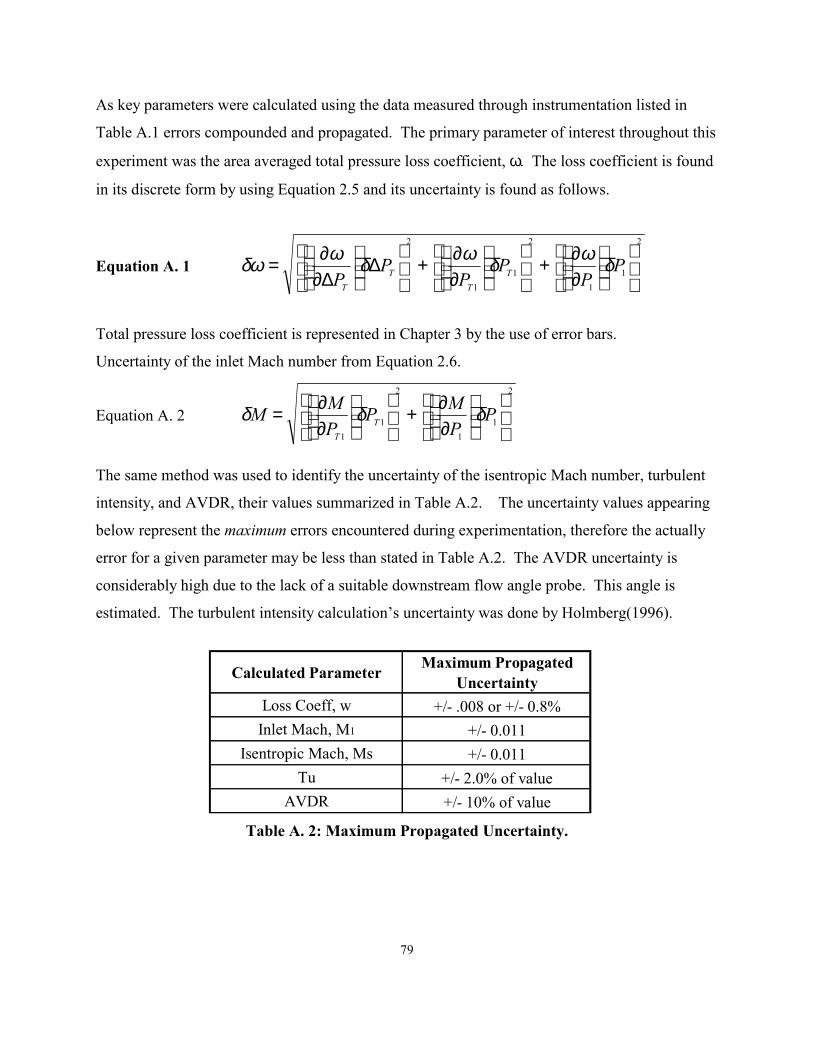
79
As key parameters were calculated using the data measured through instrumentation listed in
Table A.1 errors compounded and propagated. The primary parameter of interest throughout this
experiment was the area averaged total pressure loss coefficient, ω. The loss coefficient is found
in its discrete form by using Equation 2.5 and its uncertainty is found as follows.
Equation A. 1
2
11
2
11
2
∂∂+
∂∂+
∆
∆∂∂= P
PP
PP
P TT
TT
δωδωδωδω
Total pressure loss coefficient is represented in Chapter 3 by the use of error bars.
Uncertainty of the inlet Mach number from Equation 2.6.
Equation A. 2
2
11
2
11
∂∂+
∂∂= P
PMP
PMM T
T
δδδ
The same method was used to identify the uncertainty of the isentropic Mach number, turbulent
intensity, and AVDR, their values summarized in Table A.2. The uncertainty values appearing
below represent the maximum errors encountered during experimentation, therefore the actually
error for a given parameter may be less than stated in Table A.2. The AVDR uncertainty is
considerably high due to the lack of a suitable downstream flow angle probe. This angle is
estimated. The turbulent intensity calculation�s uncertainty was done by Holmberg(1996).
Table A. 2: Maximum Propagated Uncertainty.
Calculated Parameter Maximum Propagated Uncertainty
Loss Coeff, w +/- .008 or +/- 0.8%Inlet Mach, M1 +/- 0.011
Isentropic Mach, Ms +/- 0.011Tu +/- 2.0% of value
AVDR +/- 10% of value

80
APPENDIX B DOWNSTREAM LOSSES AND M2 VS PITCH
The following plots, are examples of the wake profiles for a given testing condition. It should be
noted that periodicity is somewhat of an issue due to lack of an effective tailboard to guide the
exit flow through the exhaust of the test section. Most recent work from other researchers at
Virginia Tech is addressing this problem and a first design iteration of a tailboard is being tested.
Figure B. 1: Sample of Downstream Loss and M2 Profiles
From Figure B.1, periodicity seems to worsen with increased cascade angle, this issue prompted
the current design and fabrication of a tailboard to correct this problem. Further tunnel
Cascade Total Pressure Loss CoefficientI=44.4o, 50% chord dow nstream, M1=0.8180
00.20.40.60.8
1
0.5 1 1.5 2 2.5Pitch
ω ωωω
average: 0.1443; AVDR=1.0884; With Tu
Cascade Exit Mach NumberI=44.4o, 50% chord dow nstream, M1=0.8180
0
0.2
0.4
0.6
0.8
1
0.5 1 1.5 2 2.5Pitch
Μ2
Μ2
Μ2
Μ2
average: 0.5473; AVDR=1.0884;w ith Tu
Cascade Total Pressure Loss Coefficientββββ1=48.4o, 50% chord dow nstream, M1=0.8149
00.20.40.60.8
1
0.5 1 1.5 2 2.5Pitch
ω ωωω
average: 0.2148; AVDR=1.0560; With Tu
Cas cade Exit M ach Nu m berββββ1=4 8 .4 o, 5 0 % chor d dow ns tr eam, M1 =0 .8 1 4 9
0
0.2
0.4
0.6
0.8
1
0.5 1 1.5 2 2.5
P itch
Μ2
Μ2
Μ2
Μ2
average: 0.4886; A V D R =1.0560;W ith Tu

81
modifications include: upstream sidewall suction and in passage sidewall suction, this will not
only make the incoming flow realistic provide a means of control for AVDR.
Figure B. 2 Loss vs Inlet Mach Number
T otal P res s u re L os s vs In let Mach N u mberOR G B lade; AVD R =0.96~1.12
0
0 .1
0 .2
0 .3
0 .4
0 .5 0 .6 0 .7 0 .8 0 .9
In let Mach Num ber
Loss
4 3 .4 degs , with T u
4 3 .4 degs , withoutT u
T otal P r es s u r e L os s v s In le t M ach Nu mberOR G B lade ; AVD R =0.96~1 .12
0
0 .1
0 .2
0 .3
0 .4
0 .5 0 .6 0 .7 0 .8 0 .9
In let Mach Num ber
Loss
4 5 .4 d e g s , w ith T u
4 5 .4 d e g s , w ith o ut T u

82
APPENDIX C HOT WIRE CALIBRATION AND REDUCTION CODE
The following excerpt is taken from Holmberg(1996) and describes the one�point calibration
theory for calculating velocities from the voltage fluctuations measured by the Hot Wire Probe.
Hot-wire calibration theory
The usual approach to calibrating a hot-wire is to place a hot-wire in a known velocity laminar jet
and to record voltage out for a given flow velocity and temperature. The data is then used in an equation
of this form:
Nu = A + B Rex
The actual values for A, B, and x will vary some, but both Bradshaw (p. 115) and Hinze (2nd ed.
p.89) give these numbers as applicable to the different Red regimes:
Nu ReTT
m
s
= +−0 17
0 450 24 0 56.
.. . for Red < 44 (3.4)
Nu ReTT
m
s
=−0 17
0 510 48.
.. for Red > 44 (3.5)
where the term Tm/Ts is a temperature correction factor, and the value of Red = 44 is where laminar to
turbulent transition of flow over the wire occurs.
At wire transition the calibration curve shifts, as seen by the changed Reynolds number exponent
(Re exponent), and the calibration curve also goes through the origin for higher Re. For typical cold
conditions in the cascade tunnel (grid tests were done in unheated flow):
Minlet = 0.36 Pt = 31.7psia = 219 kPa Tt = 290K γ = 1.4 Twire = 500K dwire = 5µm Rair = 287m2/s2K
PP
TT
t
s
t
s= +
−
=
− −1
12
2 1 1γγγ
γγ
M
which gives:

83
Ps / Pt = 0.914 Ts / Tt = 0.975 Ts = 280 K Ps = 29.0 psia = 200. kPa
then:
( )T T TP
RT
xT
Tx
U R TU d
m s w
ms
m
mm
m
air s
dm wire
m
= + =
= =
=
+
=
= =
= =
− −
/
.
. *.
* ..
..
2 390
179
1716 1027316
383 716110 556
22 6 10
121
48
51 5
6
(K)
(kg/m )
(Ns/m )
M (m/s)
Re
3
2
ρ
µ
γρ
µ
Therefore, the wire is actually operating near its transition point, but presumably in the turbulent
regime. Two assumptions were made initially:
1) Re exponent = 0.51 can be applied to the grid turbulence measurements.
2) The calibration will be a straight line through the origin if plotted as:
Nu = const*Re0.51
The above assumptions were tested experimentally and were found to be valid within the
uncertainty of measurements. A discussion of the validity of these assumptions is included in the next
section.
The result of the above two assumptions is that a calibration of a given wire can be obtained with
data at only one point (where the origin becomes the second point). Calibration of the UHW used for
performing grid turbulence field measurements was done in-situ with a calibration performed for each
tunnel run using this method. This allowed a calibration without the uncertainty of a varying tunnel total
temperature and pressure and changes in the wire itself from run to run. The specifics of this method
follow.
One point calibration methodology
As discussed above, the conditions in the tunnel for measurements behind the grids upstream of
the cascade allow for the use of this equation:
NuTT
m
s
=−0 17
0 510 48.
.. Re (3.5)
Now, each piece of this equation needs to be put into known measured quantities, and put into a
form that can lead to a useful calibration.

84
( )( )( )Nu where= = =
+
−hdk
h powerarea T
V R
R R
d L T Tm
w
w
w w w s,
( )( )( )∆
2
12
π
where the above equation for the heat transfer coefficient is taken from Freymuth and Fingerson (1980).
In this equation, HW voltage V and the tunnel static temperature Ts are the only variables. All wire
properties are considered constant given a constant temperature anemometer that in theory maintains
wire temperature and thus resistances constant. Therefore the equation for Nu reduces to:
( ) ( ) ( ) ( )Nu since ∝−
∝−
− = −VT T k
VT T k
T T T Tw s m m s m
w s m s
2 22
Then, taking the constant wire diameter out of Re, flipping the left and right hand sides of the
equation for convenience, and inserting a calibration constant:
( )ρµm
m m s m
m
s
UC V
T T kTT
=
−
−0 51 2 0 17. .
(3.6)
simplified to:
Re Nu′ = ′C (3.7)
This equation was used in the calibration of the UHW used for grid measurements. The specific
step-by-step procedure of applying these equations follows.
1. Find the average Pt, Tt, and V (HW voltage) over the selected HW sample.
2. Solve for Ts, Ps, and Tm from the above equations using γ = 1.4 as the initial value.
3. Proceed through the following equations:
Cp T x T x T x Tair s s s s= − + + −
− − −
−
1037 8 0 22371 2 8556 10 5 2694 10 5 3327 104 2 7 3 10 4
1
. . . . . (m /s K)
= 1- RCp
2 2
airγ
P P M
T T UCp
s t
s t
= + −
= −
−1 1
2
2
2 1
2
γγγ (Pa)
(K)
U M R Ts= γ ( m/s)
( )T T Tm s w= + / 2 (K)

85
ρ
µ
ms
m
mm
m
mm
m
PRT
x TT
k x TT
=
=
+
=
+
−
−
(kg/m )
(Ns/m )
(W/mK)
3
21716 1027316
383716110556
2 414 1027316
47316200
515
21 5
..
..
..
.
.
.
( )( )
Re
Nu
Re Nu
′ =
′ =−
= ′ ′
−
ρµm
m
m m s
m
s
U
V
k T TTT
C
0 51
2 0 17
.
.
/
This constant then can be used for all the HW data acquired in that run to convert bridge voltage
to a velocity series. The value of C is for a given hot-wire, and will be consistent run to run with some
small drift over time.
When using this calibration to solve for the velocity, the values of Re′ and Nu′ must be solved
iteratively at each point. The progression is similar to the above calibration equations, but the result is U
instead of a calibration constant. The method used was:
1) Solve for Cp, Ts, Tm, km, µ, γ as above.
2) Solve for Mach number, M.
3) Then Ps = f(Pt, γ, M).
4) Solve for Nu′ using the instantaneous HW voltage.
5) (ρU) = µ(C*Nu′)1/0.51, where Re′ = C*Nu′
6) Mean density from the low speed data, ρm = Ps,m/RTs
7) and then instantaneous U = (ρU)/ρm if density fluctuations are assumed negligible.
8) Iterate the above sequence until U converges.

86
The following is the Fortran Code used in the current work to generate velocities from the voltage fluctuations measured by the HW. program main real mach,nusselt OPEN(9,file='c:\temp\output.txt') OPEN(7,file='c:\temp\check.out') OPEN(5,file='c:\temp\hotfilm.txt') OPEN(6,file='c:\temp\labview.txt') r20=3.46 arfa20=0.36 rop=6.78 offset=7.0 gain=1.0 tw=(rop-r20)/arfa20*100./r20+20. tw=tw+273.15 dw=5./1000./1000. tol=0.005 c******************************************************************************************** read(5,*) number read(5,*) vhotavg write(9,30) number,vhotavg 30 format(/'number=',i7,' vhotavg=',f12.4) vhotavg=vhotavg/gain+offset read(6,*) pt read(6,*) tt read(6,*) ps read(6,*) patm write(7,40) pt,tt,ps,patm 40 format('Pt= ',f10.4,'psig ','Tt= ',f10.2,' c Ps=',f10.4, 1 'psig Patm=',f10.1,'Pa') close(7) c******************************************************************************************** pt=pt*6894.8+patm ps=ps*6894.8+patm tt=tt+273.15 mach=sqrt(5.*((pt/ps)**(1/3.5)-1)) ts0=tt/(1.0+0.2*mach*mach) velocity=mach*sqrt(1.4*287.0*ts0) tm0=(ts0+tw)/2 dens0=ps/287/tm0 visty0=1.716/100000.*(tm0/273.15)**1.5*383.716/(tm0+110.6) cond0=2.414/100.*(tm0/273.15)**1.5*473.16/(tm0+200.) reynolds=(dens0*dw*velocity/visty0)**0.51 nusselt=vhotavg**2/cond0/(tm0-ts0)*(tm0/ts0)**(-0.17) constant=reynolds/nusselt do 1000 i=1,number read(5,*) hotfilm hotfilm=hotfilm/gain+offset icount = 0 temp=constant*hotfilm**2/(tm0-ts0)/cond0*(tm0/ts0)**(-0.17) utemp=temp**(1/0.51)/dens0/dw*visty0

87
100 ts=tt-utemp**2/2/1005. sound=sqrt(1.4*287.0*ts) mach=utemp/sound tm=(ts+tw)/2 dens=ps/287/tm visty=1.716/100000.*(tm/273.15)**1.5*383.716/(tm+110.6) cond=2.414/100.*(tm/273.15)**1.5*473.16/(tm+200) nusselt=constant*hotfilm**2/cond/(tm-ts)*(tm/ts)**(-0.17) utemp1=nusselt**(1/0.51)/dens/dw*visty ut=(utemp+utemp1)/2. if(abs(ut-utemp1).le.tol) goto 900 utemp=ut icount=icount+1 if(icount.ge.10000) goto 500 goto 100 500 write(9,600) i, icount 600 format(//'i= ', i7,' icount=',i6,' error happen') 900 hotfilm=(hotfilm-offset)*gain write(9,950) hotfilm,ut 950 format(f12.4,',',f12.4) 1000 continue close(5) close(6) close(9) stop end This code was written by Shiming Li and the author, it is based on the code from Holmberg(1996).

88
APPENDIX D REDUCTION CODE FOR TURBULENCE SCALE
% Matlab M-file to reduce Hotwire Data and Perform Spectral Analysis: % Data taken on 01/27/01 using LeCroy and Labview: % LeCroy Data were sampled at 20 kHz (dt=50 us), DC offset -5V, filtered at 10kHz, 2 V FSV % Location 3: clear all; close all; %Lecroy: fsample=50000; % Sampling frequency of 50 kHz dt=1/fsample; % Sampling period (sec) N=8189; %Number of Samples 512Kx128K T=N*dt; %Total Sampling Period (seconds) df=1/T; %Frequency Resolution t=[0:dt:T]; %Define time T=(Number Samples)*(dt), dt=1/(Sampling Frequency) f=[0:df:fsample]; %Define frequency range from 0 to fsample in increments of df %Read in LeCroy data files and reduce data: load vel3.txt; hwv1=vel3(:,1); %Read first column and add back on 5 V DC component hwv2=vel3(:,2); hwv3=vel3(:,3); Vmean(1)=mean(hwv1); Vmean(2)=mean(hwv2); Vmean(3)=mean(hwv3); %PART a): DETERMINE STATISTICS: %____________________________________________________________________________________________ %Fluctuating component (a): v1=hwv1-Vmean(1); v2=hwv2-Vmean(2); v3=hwv3-Vmean(3); RMS1=(mean(v1.^2)).^0.5; RMS2=(mean(v2.^2)).^0.5; RMS3=(mean(v3.^2)).^0.5; %PART b): PLOT AUTOCORRELATION CURVE AND DETERMINE INTEGRAL LENGTH SCALE: %____________________________________________________________________________________________ %Calculate autocorrelation on each data file: Rv1=xcorr(v1,'coeff'); Rv1=Rv1(8190:16379); Rv2=xcorr(v2,'coeff'); Rv2=Rv2(8190:16379); Rv3=xcorr(v3,'coeff'); Rv3=Rv3(8190:16379);

89
%Plot autocorrelations: figure(2); plot(t,Rv1,'k',t,Rv2,'b',t,Rv3,'r'); xlabel('\tau (s)'); ylabel('Rv(\tau)'); title('Figure 1: Autocorrelation'); legend('Set 1','Set 2','Set 3'); grid on; axis([0 0.0005 -0.2 1.2]); %Perform Numerical Integration to Calculate Integral Time Scale: %Complete Data Set: First zero crossing calculated with find command: z1=find(abs(Rv1)<0.002&abs(Rv1)>=0); T1=sum(Rv1(1:z1(1)))*dt; %T is integral time scale L(1)=T1*Vmean(1); z2=find(abs(Rv2)<0.002&abs(Rv2)>=0); T2=sum(Rv2(1:z2(1)))*dt; %T is integral time scale L(2)=T2*Vmean(2); z3=find(abs(Rv3)<0.002&abs(Rv3)>=0); T3=sum(Rv3(1:z3(1)))*dt; %T is integral time scale L(3)=T3*Vmean(3); This code was written by Andrew Nix, graduate student at Virginia Tech.

90
VITA
Justin W. Douglas
Justin Douglas was born in Charleston, West Virginia on July 27, 1977. He graduated with
distinction from the Virginia Military Institute in Lexington, Virginia with a Bachelor of Science
degree in Mechanical Engineering in May of 1999. In addition to an outstanding undergraduate
academic record, he was a three year letterman in Division I football. He published his first
paper in an American Society of Engineering Education Journal in his final year at VMI. He
studied abroad at St. Catherine�s College, Oxford University in his third year at VMI. He was a
semi-finalist for the Rhodes Scholarship in the state of West Virginia in 1998. Upon the
completion of his undergraduate study he began his graduate studies at Virginia Tech under the
guidance of Dr. Wing Fai Ng. The author defended his work on March 1, 2001. Upon
graduation, the author began work at Ford Motor Company.