EFFECTS OF CO2 SATURATION ON THE RECOVERY OF THE HEAVY OIL

USING STEAM INJECTION EOR TECHNIQUE

A THESIS SUBMITTED TO

THE GRADUATE SCHOOL OF NATURAL AND APPLIED SCIENCES

OF

MIDDLE EAST TECHNICAL UNIVERSITY

BY

FARID GULUZADE

IN PARTIAL FULFILLMENT OF THE REQUIREMENTS

FOR

THE DEGREE OF MASTER OF SCIENCE

IN

PETROLEUM AND NATURAL GAS ENGINEERING

December 2014

ii

iii

Approval of the thesis:

EFFECTS OF CO2 SATURATION ON THE RECOVERY OF THE HEAVY

OIL USING STEAM INJECTION EOR TECHNIQUE

Submitted by FARID GULUZADE in partial fulfillment of the requirements for the

degree of Master of Science in Petroleum and Natural Gas Engineering

Department, Middle East Technical University by,

Prof. Dr. M. Gülbin Dural Ünver __________________

Dean, Graduate School of Natural and Applied Sciences

Prof. Dr. Mahmut Parlaktuna __________________

Head of Department, Petroleum and Natural Gas Eng.

Assist. Prof. Dr. Çağlar Sınayuç __________________

Supervisor, Petroleum and Natural Gas Eng. Dept., METU

Examining Committee Members:

Prof. Dr. Mahmut Parlaktuna __________________

Petroleum and Natural Gas Engineering Dept., METU

Asst. Prof. Dr. Çağlar Sınayuç __________________

Petroleum and Natural Gas Engineering Dept., METU

Prof. Dr. Mustafa Verşan Kök __________________

Petroleum and Natural Gas Engineering Dept., METU

Asst. Prof. Dr. İsmail Durgut __________________

Petroleum and Natural Gas Engineering Dept., METU

Dr. Sevtaç Bülbül __________________

Petroleum Research Center, METU

Date: 02.12.2014

iv

I hereby declare that all information in this document has been obtained and

presented in accordance with academic rules and ethical conduct. I also declare

that, as required by these rules and conduct, I have fully cited and referenced all

material and results that are not original to this work.

Name, Last Name: Farid, Guluzade

Signature:

v

ABSTRACT

EFFECTS OF CO2 SATURATION ON THE RECOVERY OF THE HEAVY

OIL USING STEAM INJECTION EOR TECHNIQUE

Guluzade, Farid

M.Sc., Department of Petroleum and Natural Gas Engineering

Supervisor: Asst. Prof. Dr. Çağlar SINAYUÇ

December 2014, 84 pages

Enhanced Oil Recovery processes include all methods that use external sources of

energy and/or materials to recover oil that cannot be produced economically by

conventional means.

EOR processes can be classified as: thermal methods (in-situ combustion, cyclic steam

injection, steam flooding), chemical methods (alkaline, polymer, foam, or

surfactant/polymer injection), and miscible methods (CO2, nitrogen, hydrocarbon, or

flue gas injection).

Steam flooding involves continuous injection of steam to displace oil towards

producing wells. Normal practice is to start with cyclic steam injection and to continue

with steam flooding. The mechanisms of steam injection are heating oil thus reducing

its viscosity and supplying pressure to drive the oil towards producing wells.

In this study, to analyze the effects of CO2 saturation on the heavy oil recovery by

steam injection is aimed. A synthetic model is built in Schlumberger’s software Petrel,

by using basic properties (porosity, permeability, API gravity) of hypothetical field.

vi

Production scenarios are taken to be different for better comparison of recoveries.

Sensitivity runs are conducted in Eclipse software. This study should not be compared

with real field data since a hypothetical geological model is used. Therefore, no history

match can be done in this case.

By the end of the study, water injection implementation and steam flooding are found

to be the most appropriate oil recovery techniques for this particular, hypothetical field

in terms of both production and pressure support. Therefore, scenario 1 and scenario

6 are the best methods to be applied. By the end of time schedule average reservoir

pressure for scenarios 1 and 6 are 650 psi and 464 psi respectively with 283 and 234

stb/d of production. Furthermore, for being more thorough, material balance was also

conducted in IPM tool, called MBal for checking the consistency of the model. Thus,

close pressure trend was obtained from material balance compared to simulation

model.

vii

ÖZ

CO2 DOYMUŞLUĞUNUN BUHAR BASIMI EOR TEKNİĞİ İLE AĞIR PETROL

KURTARIMINA ETKİLERİ

Guluzade, Farid

Yüksek Lisans, Petrol ve Doğal Gaz Mühendisliği

Tez Yöneticisi: Yrd. Doç. Dr. Çağlar SINAYUÇ

Aralık 2014, 84 sayfa

Geliştirilmiş petrol kurtarımı (EOR), harici enerji kaynakları ve malzemeler

kullanarak, geleneksel yöntemler ile üretilemeyen petrolün üretimini sağlayan tüm

yöntemleri içerir.

Geliştirilmiş petrol kurtarımı şu şekilde sınıflandırılabilir: ısıl yöntemler (yerinde

yanma, dönüşsel buhar basımı, buhar basımı), kimyasal yöntemler (alkalin, polimer,

köpük, veya yüzey aktif madde/polimer basımı), ve karışır yöntemler (CO2, azot,

hidrokarbon, vey abaca gazı basımı).

Buhar basımı, petrolün üretim kuyularına ötelenmesi için sürekli olarak buhar

basımını içerir. Normal uygulamaya gore önce dönüşsel buhar basımı ile başlanır ve

buhar basımı ile devam edilir. Buhar basımının mekanizması, petrolü ısıtarak

akmazlığını düşürmek ve basınç sağlayarak petrolü üretim kuyularına doğru

ötelemektir.

Bu çalışmada karbondioksit varlığının, buhar basımı ile ağır petrol kurtarımı üzerine

etkilerini analiz etmek amaçlanmıştır. Türkiye’nin güneydoğusunda bulunan Batı-

viii

Raman sahası özelliklerine benzer özellikler (gözeneklilik, geçirgenlik, API gravitesi)

kullanılarak yapay bir model oluşturulmuştur. Daha gerçekçi bir yaklaşım için Batı-

Raman petrol sahasının üretim geçmişi temel alınmıştır. Varsayımsal bir jeolojik

model kullanıldığı için bu çalışma ile gerçek saha verileri karşılaştırılmamalıdır. Bu

nedenle tarihsel çakıştırma yapılamaz.

Bu çalışma su basımı ve buhar basımı uygulamalarının bu varsayımsal saha için hem

üretim hem de basınç katkısı açısından en uygun geliştirilmiş kurtarım yöntemleri

olduğunu göstermiştir. Bunun yanısıra, modelin tutarlı olduğunu kontrol etmek için

kütle korunumu incelenmiş ve kütle korunumu ve simülasyon modeli sonuçlarının

yakın basınç yönelimine sahip olduğu görülmüştür.

ix

ACKNOWLEDGEMENTS

All praises to Almighty Allah who has never left me alone at any time in my entire

life.

I wish to express my deepest gratitude to my supervisor – Asst. Prof. Dr. Çağlar

Sınayuç for his guidance, motivation and overall for this continuous support

throughout the project. Asst. Prof. Dr. Sınayuç has spent endless hours with me to

develop the project and at this point, words are not enough to express my gratitude and

appreciation to him.

I want to acknowledge all professors and instructors, with department head, Prof. Dr.

Mahmut Parlaktuna, at the top of the list for valuable courses that are taught at Middle

East Technical University.

Finally, I want to express my deepest gratitude to family for their support, love and

understanding, which always motivates me to overcome any problem that I face in my

entire life.

x

TABLE OF CONTENTS

ABSTRACT ................................................................................................................. v

ÖZ ............................................................................................................................... vii

ACKNOWLEDGEMENTS ........................................................................................ ix

TABLE OF CONTENTS ............................................................................................. x

LIST OF FIGURES ................................................................................................... xiii

LIST OF TABLES ................................................................................................... xvii

CHAPTERS

1. INTRODUCTION ............................................................................................... 1

2. LITERATURE SURVEY.................................................................................... 5

2.1. Enhanced Oil Recovery .......................................................................... 5

2.1.1 Chemical techniques .................................................................... 5

2.1.2 Miscible displacement techniques ............................................... 6

2.1.3 Thermal EOR techniques ............................................................. 6

2.1.4 Microbial EOR methods .............................................................. 6

2.2. CO2 geological storage ........................................................................... 9

2.3. EOR CO2 .............................................................................................. 11

2.3.1 Miscible CO2 displacement method .......................................... 12

2.3.2 Immiscible CO2 displacement method ...................................... 15

2.3.3 CO2 properties ........................................................................... 16

xi

2.3.4 CO2 EOR implementation worldwide ....................................... 20

2.3.5 Comparison between miscible and immiscible CO2 flooding ... 21

2.4 Steam injection....................................................................................... 22

2.4.1 Changes in relative permeability ............................................... 24

2.4.2 Heat loss .................................................................................... 26

2.4.2.1 Heat, lost at the surface ................................................. 26

2.4.2.2 Heat, lost at the wellbore............................................... 26

2.4.2.3 Heat, lost in the reservoir .............................................. 27

2.4.3 Types of steam injection ............................................................ 28

2.4.3.1 Cyclic steam injection ................................................... 28

2.4.3.2 Continuous steam injection ........................................... 30

2.4.4 Selection criteria ........................................................................ 32

2.4.5 Variations and optimization of steam injection ......................... 32

2.4.5.1 Steam flooding prior to water injection ........................ 32

2.4.5.2 Water alternating steam ................................................ 33

2.4.5.3 Air injection after steam injection ................................. 33

2.4.5.4 Hybric steam techniques ............................................... 33

2.4.5.5 Fracturing with steam.................................................... 34

2.4.6 Steam injection implementation worldwide .............................. 34

2.5 Modeling of CO2 injection and steam injection ..................................... 35

2.5.1 Immiscible CO2 injection simulation ........................................ 35

xii

2.5.2 Steam injection simulation ........................................................ 36

3. STATEMENT OF THE PROBLEM ..................................................................... 39

4. METHODOLOGY ................................................................................................. 41

4.1 Model setup ............................................................................................ 41

4.2 Field history ........................................................................................... 42

4.3 Sensitivity runs ...................................................................................... 45

4.4 Scenarios ................................................................................................ 46

4.5 Material balance ..................................................................................... 48

5. RESULTS AND DISCUSSIONS .......................................................................... 51

5.1 Base case ................................................................................................ 51

5.2 Scenarios ................................................................................................ 53

5.3 Comparison of all scenarios ................................................................... 59

5.4 Effect of CO2 on steam injection ........................................................... 67

5.5 Effect of water injection wells ............................................................... 68

5.6 Material balance check ........................................................................... 71

6. CONCLUSION ................................................................................................... 77

REFERENCES ................................................................................................... 79

xiii

LIST OF FIGURES

FIGURES:

Figure 2.1 Depth vs. density of CO2..…………………………………… ................ 10

Figure 2.2 a) good recovery, b) viscous fingering ..................................................... 12

Figure 2.3. A schematic view of water alternating gas process of miscible CO2

injection ...................................................................................................................... 14

Figure 2.4. Schematic view of immiscible CO2 injection ......................................... 15

Figure 2.5. Phase diagram of carbon dioxide ............................................................. 17

Figure 2.6. Density of CO2 with respect to temperature and pressure ...................... 17

Figure 2.7. Compressibility of CO2 with respect to pressure and temperature .......... 18

Figure 2.8. Viscosity of CO2 with respect to temperature and pressure ................... 18

Figure 2.9. Development of CO2 displacement techniques and cumulative rates in

USA ........................................................................................................................... 21

Figure 2.10. Viscosity of 4 oil samples under different temperatures ...................... 23

Figure 2.11. Effect of temperature on relative permeability ..................................... 24

Figure 2.12. Heat content of boiling water and dry saturated steam at different

pressure ..................................................................................................................... 25

Figure 2.13. Heat loss in the wellbore in comparison with injection rate ................. 27

Figure 2.14. Variation of heat losses to the formation with formation thickness ...... 28

Figure 2.15. Huff and puff method ........................................................................... 29

Figure 2.16. Steam assisted gravity drainage ............................................................ 30

xiv

Figure 2.17. SAGD technique in Tangleflags formation .......................................... 31

Figure 4.1. Grid model ............................................................................................... 43

Figure 4.2. Oil relative permeability .......................................................................... 44

Figure 4.3. Gas relative permeability ......................................................................... 44

Figure 4.4. Water relative permeability ..................................................................... 45

Figure 4.5. All well are producers .............................................................................. 46

Figure 4.6. Central well is injection CO2/steam ......................................................... 46

Figure 5.1 Field daily oil production rate ................................................................... 52

Figure 5.2 Average reservoir pressure ....................................................................... 52

Figure 5.3 Field daily water production rate .............................................................. 53

Figure 5.4 Comparison of base case and scenario-1 average reservoir pressure ....... 54

Figure 5.5 Comparison of base case and scenario-1 oil production rate .................... 54

Figure 5.6 Comparison of base case and scenario-1 water production rate ............... 55

Figure 5.7 Comparison of base case and scenario-2 average reservoir pressure ....... 55

Figure 5.8 Comparison of base case and scenario-2 oil production rate .................... 56

Figure 5.9 Comparison of base case and scenario-3 average reservoir pressure ....... 56

Figure 5.10 Comparison of base case and scenario-3 oil production rate .................. 57

Figure 5.11 Comparison of base case and scenario-3 water production rate ............. 57

Figure 5.12 Comparison of base case and scenario 4 oil production rate .................. 58

Figure 5.13 Comparison of base case and scenario-5 oil production rate .................. 58

Figure 5.14 Comparison of base case and scenario-6 oil production rate .................. 59

xv

Figure 5.15 Comparison of field average reservoir pressure ..................................... 60

Figure 5.16 Comparison of field oil production rates ................................................ 61

Figure 5.17 Comparison of cumulative oil production rates ..................................... 62

Figure 5.18 Comparison of water production rates .................................................... 62

Figure 5.19 Reservoir temperature distribution for scenario-6 september 1963 ....... 63

Figure 5.20 Reservoir temperature distribution for scenario-6 june 2016 ................. 64

Figure 5.21 Reservoir pressure distribution for scenario-6 ........................................ 65

Figure 5.22 Viscosity distribution for scenario 6 ....................................................... 66

Figure 5.23 Effect of water injection and CO2 injection before steam injection on oil

production rate ........................................................................................................... 67

Figure 5.24 Effect of water injection and CO2 injection before steam injection on

cumulative oil production .......................................................................................... 68

Figure 5.25 Proximity of well locations ..................................................................... 69

Figure 5.26 Water production .................................................................................... 70

Figure 5.27 Oil production ......................................................................................... 70

Figure 5.28 Reservoir and wells................................................................................. 71

Figure 5.29 Input paameters for material balance ...................................................... 72

Figure 5.30 PVT inputs .............................................................................................. 72

Figure 5.31 Production inputs from simulation outputs............................................. 73

Figure 5.32 Cumulative injection, production and reservoir pressure ....................... 73

Figure 5.33 Matching uncertaion parameters............................................................. 74

Figure 5.34 Average reservoir pressure comparison between material balance and

simulation ................................................................................................................... 75

xvi

Figure 5.35 Drive mechanism .................................................................................... 75

xvii

LIST OF TABLES

Table 2.1 Approximate criteria for enhanced oil recovery techniques ..................... 7,8

Table 2.2. Amount of CO2-eor projects and rates ...................................................... 20

Table 2.3. Essential characteristics of miscible and immiscible projects. ................. 22

Table 2.4. Recovery of different thermal EOR processes .......................................... 35

Table 4.1 Main parameters ......................................................................................... 42

Table 4.2. Well locations in the grid model ............................................................... 45

Table 5.1 The summary of the simulation cases ........................................................ 51

Table 5.2 Average oil production rate........................................................................ 60

Table 5.3 Water injection scenarios ........................................................................... 69

xviii

1

CHAPTER 1

INTRODUCTION

Crude oil is found in underground deposits that have migrated there millions of years

ago. It is defined as a hydrocarbon mixture in liquid state. As name implies,

hydrocarbons mainly consists of hydrogen and carbon. However, impurities such as

nitrogen, oxygen, metals and sulphur are also contribute to the composition of crude

oil. Production as well as physical and chemical properties of crude oil are influenced

by its composition.

Source rock plays an essential role in formation of petroleum. It is the fine-grained,

organic rich rock that is responsible for generation of petroleum. Crude oil is expelled

from source rock once it is fulfilled. Mainly, there are three driving forces of migration,

which are buoyancy, water flow and capillary pressure. Migration of petroleum

finishes either on the surface or may be stopped by impermeable rock underground

called cap rock. In this case oil is trapped in reservoir rock. Reservoir rock itself is a

porous and permeable rock from where crude oil is extracted.

The history of petroleum industry clearly demonstrates that there are three main

production stages: primary recovery, secondary recovery, and enhanced oil recovery

(EOR) or tertiary recovery.

In the onset of petroleum production, which has started in 1840s, due to the absence

of technology people rely only on primary production, which means that petroleum

comes to surface by means of reservoir energy. Main principle of producing petroleum

in this stage is pressure difference between reservoir and sandface of a well that drives

oil. In primary stage there are several driving forces, which pressurize reservoir. Main

driving forces are: solution gas drive, water drive (aquifer), and gas-cap drive.

2

The fraction of hydrocarbon that can be extracted by primary recovery is generally in

between 5% to 15% (Tzimas and Peteves, 2003).

The end of primary stage and start of secondary recovery stage is at such point of

reservoir lifetime when reservoir pressure is so low that there is not sufficient energy

to produce hydrocarbons to the surface. The main aim of secondary recovery is to

provide energy to reservoir for increasing surface production. There are two main

techniques of secondary recovery: water injection (water flooding) and gas injection.

Due to the fact that aquifers are always present, water is preferred during the secondary

recovery stage. Basically there are two main purposes of water flooding: pressurizing

the reservoir (increasing the reservoir energy) and displacement of hydrocarbons

towards production wells. By the end of secondary recovery the overall fraction of

extracted hydrocarbons is about 35% - 45% (Tzimas and Peteves, 2003).

At some point of production by water injection, there is a moment when production

drops so low that it becomes unprofitable, in economical perspectives, to continue the

production. Therefore, in order to produce the remaining oil that cannot be recovered

by secondary recovery mechanisms, an enhanced oil recovery technique is

implemented, that uses external energy sources for increasing oil mobility, so that oil

can easily flow through the reservoir towards the producing wells and to the surface.

Enhanced Oil Recovery is classified as thermal recovery (steam flooding, in-situ

combustion, etc.), chemical recovery (alkaline, polymer, etc.) and miscible recovery

(CO2, nitrogen, etc.)

EOR techniques increase microscopic oil displacement and volumetric sweep

efficiencies, which, in its turn, leads to mobilization of oil within the field.

This study is mainly concentrated on CO2 injection and steam flooding applications.

Therefore in following paragraphs these techniques will be explained.

One of the most common tertiary recovery methods is CO2 EOR. Beyond primary and

secondary recovery stages, an additional 5% to 20% of oil can be recovered by CO2

injection. Mainly CO2 is produced from underground deposits and can also be

produced from electric power plant emissions. Once CO2 is produced, it is transported

to the field mainly by pipes. During water injection stage, oil is pushed towards

3

producing wells by means of pressure through straight force. The situation in CO2

injection differs. CO2 has a property to dissolve in oil, which implies that CO2 increase

miscibility. Once CO2 is injected to the reservoir, it starts to dissolve in oil and swelling

process starts (oil expands). After absorption of CO2 in the zone of miscibility the oil

viscosity is reduced and it can flow easily throughout the reservoir. The main problem

in CO2 injection is that, due to the fact that CO2 viscosity is much lower than oil’s,

CO2 can start to form channels towards production wells. This indicated that, in this

case, CO2 can leave huge amount of oil bypassed.

If the oil gravity is low, steam injection is one of the most appropriate enhanced oil

recovery methods to be used. Since oil has low gravity, which means that it is viscous,

steam is injected to the reservoir to reduce its viscosity, so that oil can comparatively

easily flow throughout the formation. Another advantage of steam injection method is

that, as in the case of water injection, it supplies additional pressure and help to push

oil towards the production wells. The most important advantage of steam flooding is

that it can be injected to different kind of reservoirs. However there are also some

restrictions of this method, which are: depth and formation thickness. The main reason

of using steam instead of heated water is that in case of steam injection less water

would be produced, which in its turn implies that more heat would remain in the

reservoir. One of the main differences between carbon dioxide and water in reservoir

conditions is that water is immiscible with oil, which means that the main purpose of

water flooding is to push oil towards producing wells and pressurize the reservoir.

However, there are two methods of CO2 injection: one of which is miscible flooding,

the purpose of which is to dissolve in oil and reduce its viscosity as well as for oil

swelling, and the second one is immiscible CO2 injection, which does not dissolve in

oil. Therefore, the goal of immiscible CO2 flooding is to create a gas cap, which will

lead to reservoir pressure support.

After injection of CO2 for a long time in a reservoir, the CO2 saturation increases. The

effects of CO2 saturation on the recovery by steam injection are studied by using a

reservoir model. Main parameters as porosity, permeability and API gravity are taken

to be appropriate for heavy oil fields with production scenarios implemented in the

majority of the reservoirs worldwide.

4

In this study, the geological model is built and populated using Schlumberger’s Petrel

Software. Main parameters to be considered for populating the simulation model are

permeability, porosity, net to gross (NTG) ratio, and pressure volume temperature

(PVT) data. The model has an anticline structure. For production and injection

purposes 5-spot well structure was chosen to see the field performance.

After the model is prepared, sensitivity runs were conducted. One of the purposes is

to see how CO2 injection affects production with steam injection, which implies that

the only parameter to be taken into consideration as an outcome is oil recovery by

different scenarios. However, some other scenarios are also evaluated as well. For

instance, the model is run with steam flooding immediately after water injection.

Continuation of CO2 injection scenario is also considered. History matching cannot be

applied in this study as only porosity, permeability, API gravity are applied from real

reservoir. Production scenarios are taken to be representative to heavy oil reservoirs.

All input data are taken hypothetically. However, material balance equation is also

used for this study in order to see the consistency of the simulation model.

5

CHAPTER 2

LITERATURE SURVEY

2.1 Enhanced Oil Recovery Methods

Enhanced Oil Recovery (EOR) includes a vast majority of techniques implemented to

increase production, one of which is CO2 flooding. After primary and secondary

recovery processes rock and oil parameters as well as saturations are going to be

known in each special case. These differences in reservoir characteristics play an

important role in selection of enhanced oil recovery methods for continuation of

production from existing fields. An appropriate EOR technique is chosen based on

reservoir porosity/permeability, oil structure and mainly accessibility of sufficient

amount of material required for EOR method. Generally, summarizing mentioned

aspects of selecting EOR technique, main role is played by economics of the project

to be implemented (Green and Willhite, 1998). EOR techniques will be discussed

shortly:

2.1.1. Chemical techniques:

The main purpose is to inject surfactants and/or alkaline for reduction of capillary

forces which negatively influence the motion of oil in the reservoir. Generally

speaking, it enhances microscopic and macroscopic sweep efficiency. The best

reservoirs for surfactant or alkaline injection are fields which are heterogeneous but

with good permeability.

Another chemical process consists of addition of polymer to water, which is injected

into the reservoir. Existence of polymers in water decrease its mobility, thus better oil

sweep can be achieved.

Due to the fact that mentioned techniques are hard to control, they are mainly

implemented in the final stage of the recovery.

6

2.1.2. Miscible displacement techniques:

Miscible displacement techniques include injection of any kind of fluid that will

dissolve in oil. The purpose of these techniques is to inject a gas in order to achieve

miscibility with oil. Once it is achieved, capillary forces will be reduced as well as oil

will become less viscous, which in its turn would lead to better/easier movement of oil

within the porous media. Miscible displacement techniques include injection of

nitrogen, methane, flue gases, etc.

2.1.3. Thermal EOR techniques:

Thermal EOR techniques are implemented to increase reservoir temperature to achieve

a decrease in oil viscosity. In order to increase reservoir temperature, steam and/or hot

water are injected or even some portion of oil in the reservoir is burned. Thermal EOR

techniques are implemented mainly for the reservoirs with heavy oil. Microwave EOR

consists of sending of microwaves to the reservoir, which would heat up oil, thus

reduce its viscosity for better motion.

2.1.4. Microbial Enhanced Oil Recovery methods:

The basic function of microbial EOR technique is to increase oil recovery by the

mobilization of oil in the reservoir that is manipulated by microorganisms and this

leads to better sweep efficiency. By means of microbial EOR it is possible to produce

up to 60% of the remaining oil (Sen, 2008).

A simple list of parameters that would help to identify which EOR technique to

implement is shown in Table 2.1.

7

Table 2.1. Approximate criteria for Enhanced Oil Recovery techniques (Green et al., 1998)

Gravity (oAPI)Viscosity (cp) Composition Oil Saturation (%)

>22 (36) <10 (1,5) High % of C5- C12 >20 (55)

>35 (48) <0,4 (0,2) High % of C1- C7 >40 (75)

>23 (41) <3 (0,5) High % of C2- C7 >30 (80)

Miscible Gas Injection Methods

Chemical methods

Thermal methods

Steam >8 (13,5) <20000 (4700) N.C. >40 (66)

Combustion >10 (16) <5000 (1200) Asphaltic components >50 (72)

CO2

Nitrogen/ Flue gases

Hydrocarbon (e.g. N. gas)

Miccelar/ Alkaline/ Polymer Flooding >20 (35) <35 (13) Light & Intermediate >35 (53)

EOR Method

Oil Properties

8

Table 2.1. (cont). Approximate criteria for Enhanced Oil Recovery techniques (Green et al., 1998)

Net thickness (m) Average permeability (mD) Depth (m) Temperature(oC)

Wide range Not critical >833 Not critical

Thin Not critical >2000 Not critical

Thin Not critical >1333 Not critical

Combustion

Steam

Reservoir Properties

Miscible Gas Injection Methods

Chemical methods

Thermal methods

EOR Method

CO2

Nitrogen/ Flue gases

Hydrocarbon (e.g. N. gas)

Miccelar/ Alkaline/ Polymer Flooding

7 >200 <1500 (500) Not critical

>3 >50 <3833 (1167) >38 (60)

Not critical >10 (450) <3000 (1083) <90 (26)

9

2.2 CO2 Geological Storage

According to Global CCS Institute our planet has an atmosphere that consists mostly

of nitrogen and oxygen, but there are also some little amounts of other gases like noble

gases (argon, helium, neon and kripton), hydrogen and greenhouse gases. Greenhouse

gases themselves include: water vapor (H2O), carbon dioxide (CO2), methane (CH4),

etc. However CO2 itself accounts of more than 77 percent of anthropogenic emissions.

It has been observed that CO2 has a huge thermal impact to the climate of the Earth. It

is also known as greenhouse effect.

Greenhouse effect makes the life to be possible on the planet. However, the

concentrations should be stable within the atmosphere. An unexpected decrease of

CO2 may cause the Earth to come to next ice age, on the other hand a sudden increase

in CO2 concentration would lead to global warming. Occurrence of both ice age and

global warming has been seen in the history of the Earth. Today, ratio of atmospheric

temperature to CO2 content is higher than ever seen for last 4000 years because; natural

processes of the Earth cannot come up with such high concentration of emissions.

Scientists proved that due to high CO2 emissions the planet is going to enter next global

warming the evidence of which is a process of ice caps melting. Today, world CO2

emissions are about 36000 tons/year (Blok K, et.al 2012). Bryngelsson et al. (2009)

explained that in order to reduce carbon amount in the atmosphere it was proposed to

capture and store CO2, because it seems to be one of the most appropriate and

immediate way of mitigation the climate change. The technology involves capturing

CO2 at the place where it is emitted by plants, transportation of CO2 by pipelines to

the storage, where it is compressed and injected to the underground reservoir at depths

deeper than 800 meters. The reason of why CO2 is compressed and injected deeper

than 800 meters is for CO2 to become supercritical fluid. On one hand supercritical

fluid behave as a gas, so that it easily diffuse through pores. On the other hand it also

behaves as a liquid because it occupies less space in comparison with gases. 800 meters

is the minimum depth and 72.9 atm. is the minimum pressure at which supercritical

fluid can exist.

10

Figure 2.1. Depth vs. density of CO2 graph (West Virginia carbon sequestration,

2008)

Once CO2 is injected into an underground reservoir its volume is compressed to circa

500 times smaller, than at the surface. The main purpose of carbon capture and storage

(CCS) is to close a circle. It starts from coal, petroleum extraction, continue with

combustion factories, plants and closing up with capture of CO2, transportation,

injection and storage underground.

The main question in this case is where these geological storages to be located so that

it will be safe and secured. Sedimentary basins are thought to be a reliable place for

CO2 storage, due to the high permeability. According to Burruss (2004) oil and gas

reservoirs can store carbon dioxide safely for a long time. The seal of oil and/or gas

reservoirs have proved to be effective, preventing oil and gas to escape. Moreover,

injection of CO2 for storage purposes would pressurize the reservoir and increase

production of oil. Identically in natural gas fields production would also be increased

once CO2 is injected to the reservoir (Oldenburg et al., 2001). Reservoir rocks can be

a good medium to store CO2. The reason is that reservoir rocks are porous and

11

permeable so that CO2, being in a liquid state, can easily spread in it. Furthermore,

there is a seal rock (cap rock) just above reservoir rock, which is impermeable,

therefore fluid cannot escape reservoir up to the surface.

Salt waters found in sandstone formations are characterized to have greater volume for

CO2 storage. Nevertheless, based on Burruss (2004) the main problem linked to

mentioned formations is their low permeability.

2.3 EOR CO2

Based on observations, a significant portion of oil originally in place still remains

within a reservoir after secondary recovery process. In areas influenced by water

during secondary oil recovery, the saturation of rock with crude oil is around 15 to

35% (Sunnatov, 2010). On the other hand, in unswept regions saturation can be

extremely higher. Therefore, an effective EOR technique should be selected which

will lead to mobilization of oil left in the reservoir and also to formation of sufficient

oil volume that will easily move towards producing wells. Mobilization of oil can be

accomplished by CO2 injection. Once CO2 is injected to the reservoir physical and

chemical reactions take place and leads to interaction of CO2 with rock and fluid. This

process builds suitable conditions that increase oil recovery. The conditions mentioned

are: 1) reduction of interfacial tension among rock and oil which will lead to easier

flow of oil within pores by decrease in capillary forces, 2) CO2 dissolve in oil, thus, it

expands in volume (swelling) as well as oil viscosity will be decreased (ECL

Technology Report 2, 2001).

Usually companies are trying to increase oil production by minimum usage of CO2.

There are two ways of getting CO2: firstly from a natural CO2 source and secondly by

capturing carbon dioxide from an emission source. This CO2 will be injected back on

a successive way. Second one is to buy CO2. Through economical evaluations,

companies decide whether recycling is cheaper or purchasing of carbon dioxide.

Generally, acquisition of CO2 prior to injection comes up to 50-80% in all proceeding

CO2-EOR operations (Schulte, 2004). Therefore, operating companies look for

producing most of injected CO2 from the production well within the oil. Once CO2 is

produced, it is separated, pumped to the injection area of the field and together with

fresh CO2 injected to the reservoir.

12

However, nowadays based on economic and ecological perspectives, CO2 geological

storage operations are rising to be important as well. This implies that in recent future

CO2 injection will play two essential roles, which are increasing oil recovery as well

as underground storage.

2.3.1. Miscible CO2 displacement method

Goodwear et al. (2003) claimed that under suitable circumstances, when pressure,

temperature and composition of oil are adequate, it is possible to obtain a miscible CO2

with oil. It means that CO2 will dissolve in oil and a mixture of petroleum and CO2

will move as a single-phase liquid within the reservoir. Consequently, oil-swelling

process takes place, viscosity reduces as well as interfacial tension decreases.

Once CO2 is injected it does not mix with oil immediately. Reservoir fluid composition

changes once CO2 is injected and that leads to development of miscible carbon

dioxide. A process of miscibility of CO2 with oil is called as Multiple Contact

Miscibility (MCM). A slight change in oil structure/composition creates miscibility

among oil and carbon dioxide. However, in real life situation interaction of CO2 and

oil is not as simple as it is thought.

Figure 2.2. a) good recovery, b) viscous fingering (Conaway et al. 1999)

Figure 2.2 shows two different situations that can happen while CO2 injection. In the

left side recovery will increase drastically due to strong and steady front of CO2 and

oil, which sweep oil towards producing well. On the other hand, in the right side

viscous fingering emerges. Viscous fingering occurs due to the channels and/or cracks

13

through which CO2 bypasses oil and consequently reachs production wells, leaving

huge amount of oil within the reservoir.

Pressure is mainly responsible for the development of miscibility of CO2 in oil. For

carbon dioxide to be able to entirely mix with oil, a Minimum Miscibility Pressure

(MMP) is obligatory. In other words, as mentioned earlier, on the surface CO2 is

compressed to supercritical state and injected to the depth more than 800 meters, so

that it remains in supercritical state within the reservoir. This implies that for

successful sweep of oil by miscible CO2, injection pressure must be larger than MMP

as well as less than reservoir pressure. Thus, MMP plays an essential role for reliable

implementation of miscible CO2 displacement method for increasing oil recovery.

From theoretical point, it is possible to recover oil which has influenced by CO2.

However, the situation is not so smooth in real life situations. Based on experience,

CO2 injection provides only 5-20% oil recovery (Goodwear et al., 2003). Problems

that cause the reduction of recovery are:

1) A certain distance for flowing of carbon dioxide within the reservoir is required

for CO2 to become miscible.

2) Existence of cracks and fractures in the reservoir may manipulate flow of CO2 to

be unstable. In this case, due to high velocity and low viscosity, carbon dioxide

will flow faster towards producing well and leads to viscous fingering.

3) By gravitational forces due to different density of oil and CO2, the latter reaches

producing well easier.

4) Prior to CO2 EOR, water injection technique is basically implemented. Not all

water is produced by the end of injection. Some water remains in the reservoir.

Some energy of CO2 is spent to the mobilization of remaining water.

In order to prevent problems mentioned above, CO2 is usually mixed up with water

and injected to the reservoir, which is called Water Alternating Gas technique (WAG).

The purpose of addition of water is due to fact that water is more reservoir-friendly

and spreads more steadily within the reservoir, thus, increasing recovery.

14

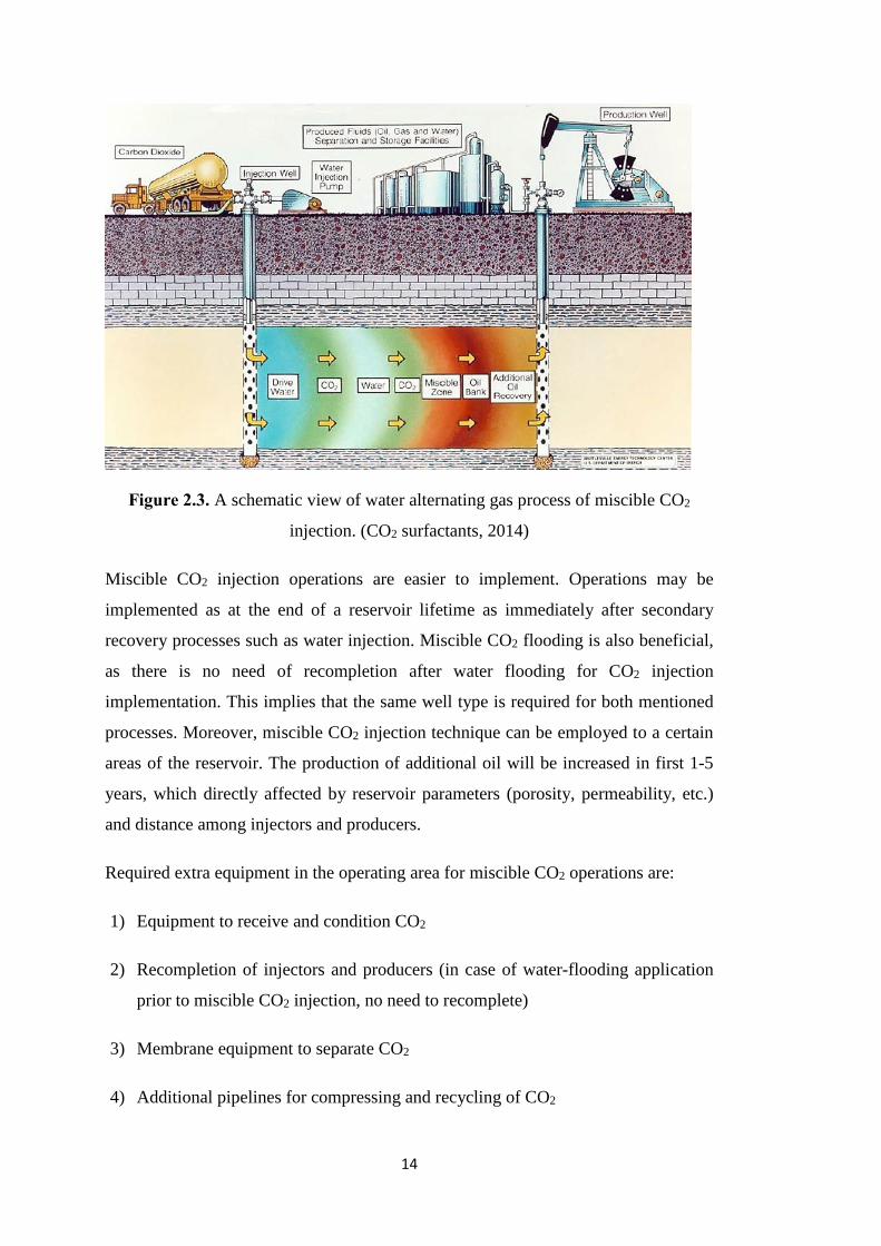
Figure 2.3. A schematic view of water alternating gas process of miscible CO2

injection. (CO2 surfactants, 2014)

Miscible CO2 injection operations are easier to implement. Operations may be

implemented as at the end of a reservoir lifetime as immediately after secondary

recovery processes such as water injection. Miscible CO2 flooding is also beneficial,

as there is no need of recompletion after water flooding for CO2 injection

implementation. This implies that the same well type is required for both mentioned

processes. Moreover, miscible CO2 injection technique can be employed to a certain

areas of the reservoir. The production of additional oil will be increased in first 1-5

years, which directly affected by reservoir parameters (porosity, permeability, etc.)

and distance among injectors and producers.

Required extra equipment in the operating area for miscible CO2 operations are:

1) Equipment to receive and condition CO2

2) Recompletion of injectors and producers (in case of water-flooding application

prior to miscible CO2 injection, no need to recomplete)

3) Membrane equipment to separate CO2

4) Additional pipelines for compressing and recycling of CO2

15

5) Gauges to monitor.

2.3.2. Immiscible CO2 displacement technique

According to Kulkarni (2003) in some instances of heavy oil reservoirs or in the

reservoirs with low reservoir pressure, it is still possible to increase production with

CO2 injection, despite Minimum Miscible Pressure is not achieved. In this case CO2

is not miscible. However, some portion of oil still swells, as certain amount of CO2

will be dissolved in oil, due to high injection pressures. Theories imply that injection

of CO2 to the reservoir containing heavy oil may lead to a considerable reduction of

its viscosity. However, this is not the main goal of immiscible CO2 flooding. As in

case of water flooding, the main purpose of immiscible CO2 injection is to keep or

even increase reservoir pressure. Water flooding is more effective technique in

comparison with immiscible CO2 injection, as water has an ability to spread more

uniformly throughout the reservoir. Therefore, immiscible CO2 injection technique has

only been used in few cases, when geologic parameters or permeability are not

appropriate for water injection. The crest is the best part of the reservoir where CO2 is

injected and where it starts to feel the pore volume. Immiscible CO2 injection looks

like gas injection of secondary recovery technique. As oil is heavier than carbon

dioxide, the latter starts to gather at the top of the trap, hence creating a gas cap that

consequently push oil downward, towards production well (Figure 2.4).

Figure 2.4. Schematic view of immiscible CO2 injection (Tzimas et al, 2005)

16

Due to the fact that water slows down the motion of oil in the reservoir, it is not

recommended to implement immiscible CO2 flooding after water injection, as the

latter would stop the effectiveness of immiscible CO2 injection.

The implementation of immiscible CO2 injection can rarely be seen nowadays, due to

the undesirable economical aspects. A requirement of a huge amount of CO2 as well

as certain quantity of new wells will not be compensated by a little and slow oil

recovery. Until additional oil is produced, ten years of injection may be required.

Moreover, implementation of immiscible technique in a certain part of the reservoir is

impossible, which means that immiscible technique can generally be applied to the

whole reservoir (Green, 2003).

However, after an international agreement of Kyoto protocol, carbon capture and

storage (CCS) is becoming to be under interest. Immiscible displacement schemes can

store significant amounts of CO2 underground, which may play an essential role in

decision-making. As we know, in miscible displacement techniques CO2 left in the

reservoir depends on the amount of it dissolved in oil and produced to the surface.

However, in immiscible displacement projects the amount of CO2 retained in the

reservoir is dictated by the reservoir pore volume. Moreover, in miscible CO2 injection

technique breakthrough cannot be avoided, but with correct project design it is possible

to exclude such breakthrough in case of immiscible displacement (Kulkarni, 2003).

2.3.3. CO2 Properties

Simple carbon dioxide has no color and cannot be smelled. It is an inert gas which

cannot be burned. The molecular weight of CO2 is 1.5 times greater than that of air. In

spite of the fact that carbon dioxide is more temperature dependent, pressure also plays

an important role in its physical properties. Solid form of carbon dioxide can be

reached at low temperatures and pressures. Once mentioned parameters start to be

increased solid CO2 transforms to liquid one. There is also a point when gaseous, liquid

and solid CO2 are in equilibrium. This point is called a triple point (Figure 2.5).

17

Figure 2.5. Phase diagram of carbon dioxide (Baviere, 1980)

CO2 phase behavior can also be expressed based on density, compressibility, viscosity.

Figure 2.6. Density of CO2 with respect to temperature and pressure (Holm, 1987)

As can be seen in Figure 2.6, when temperature is above critical positions, increase in

pressure causes an increase in the density. However, unexpected disturbances appear

once temperature falls below the critical conditions.

18

Figure 2.7. Compressibility of CO2 with respect to pressure and temperature

(McQuarrie, Donald A. (1999))

Figure 2.7 shows compressibility behavior of carbon dioxide, natural gas and mixture

of CO2 and methane.

Figure 2.8. Viscosity of CO2 with respect to temperature and pressure (Lee,

A.L.et.al .1966)

19

From Figure 2.8 above it can be noted that viscosity of carbon dioxide depends on

pressure and temperature. In case of a constant reservoir temperature, increase in

pressure will lead to viscosity build up.

Awareness of physical properties of carbon dioxide is essential, especially in case of

CO2 flooding operations. It is usually assumed that injected carbon dioxide enters the

formation in supercritical state. This implies that CO2 pressure and temperature are set

properly. However, during injection processes CO2 is injected in a liquid state due to

simplicity in operations compared to supercritical carbon dioxide. Nevertheless,

problems may occur in this case as well. For instance, thermal stresses influenced by

carbon dioxide and/or phase changes within the tubing, formation may lead to the

occurrence of some problems. Liquid carbon dioxide is more effective to be injected

than supercritical one, due to the fact that the density of the latter is less than that of

CO2 in liquid state. Therefore, injection of liquid CO2 would lead to less overpressure

as in surface so in the reservoir.

After initialization of injection the process of heat transfer takes place as in tubing so

in the formation. According to Lu and Connell (2008) lateral heat transfer occurs in

the tubing and it is represented by formula:

𝑄 = −2𝜋𝑅𝑝𝑈∞(𝑇 − 𝑇𝑔𝑒𝑜(𝑧)) (1)

In this formula 𝑈∞ is the parameter showing heat transfer. It includes all properties of

injection well and fluid which is injected through it. The radius of the injection well is

represented by 𝑅𝑝 . Geothermal temperature throughout the pipe is set as 𝑇𝑔𝑒𝑜(𝑧).

Thermal characteristics of parts of injection well play a key role in heat transfer

coefficient behavior. Of course, time and temperature are also responsible for changes.

However, temperature plays a considerable role only in case of high temperatures,

otherwise, little impact will be on overall heat transfer coefficient.

As mentioned earlier, CO2 is injected in liquid state and transformed into supercritical

one at the bottom hole. In order to keep liquid CO2 from outer formations’ heat, tubing

is recommended to thermally insulate. Thermal insulation of pipe would lead to overall

heat transfer coefficient to be reduced, which leads to relatively lower temperatures.

Thus, density of liquid carbon dioxide will be close to that of water in tubing.

20

Basically, the ability of an item to conduct heat is called heat conductivity. Higher

thermal conductivity of an item, bigger the amounts of heat transfer to the surrounding

medium. Therefore for thermal insulation purposes items with lower thermal

conductivity are used. On the other hand, materials with higher thermal conductivity

are used when spreading of heat into surrounding items is required. Thermal

conductivity depends mainly on temperature. Thermal conductivity of CO2 at

temperature of 25°C is 0.0146 W/(m K).

2.3.4. CO2-EOR implementation worldwide

Based on Schulte (2004), CO2-EOR has proved to be a successful project worldwide

for increasing oil recovery. Generally, most of CO2 injection operations have been

undertaken in North American onshore fields. In 2004 there were 79 CO2 injection

projects in the world. Share of the USA were 70 miscible CO2 injection operations and

1 immiscible, while the rest are shared between Canada with 2 miscible projects,

Trinidad with 5 immiscible carbon dioxide injections and Turkey close this chain up

with one immiscible displacement operation in Bati Raman oil field (Table 2.2).

Table 2.2. Amount of CO2-EOR projects and rates (Moritis, 2006)

Country

Project

Type

No of

projects

Production rate

(stb/day)

USA Miscible 70 205775

Immiscible 1 102

Canada Miscible 2 7200

Turkey Immiscible 1 6000

Trinidad Immiscible 5 313

The approximate oil production from these 79 CO2 injections in 2004 was about 230

Mstb/day, which account to 0.3% of oil produced worldwide. Implementation of

miscible CO2 injection took place in the North Sea only once, when carbon dioxide

was injected to the Egmanton oilfield. However, this project was terminated later due

to insufficient injection rates.

Undoubtedly, with 94% of CO2 injection implementation, USA stands in the first

place. A rapid increase in oil recovery with CO2 has been started from 1980s. In 2004,

21

CO2-EOR accounted for 31% of all produced oil in the USA in comparison with rest

of the EOR techniques and 3.5% of the total recovery (Schulte, 2004). Two biggest

CO2 injection projects implemented in the USA were Wasson-Denver and Means

projects where recoveries were 41 Mstb/day and 7.2 Mstb/day respectively. Sacroc

field which is located in Permian basin is best known in petroleum industry where first

miscible CO2 injection technique was implemented in 1972. Afterwards a slight

increase in CO2-EOR can be noticed until 1990th, when application of CO2

displacement methods have rapidly increased in spite of the fact that oil was cheap.

Generally, three important changes played an essential role in an increased

implementation of CO2-EOR: 1) Due to development in technology production costs

were reduced, 2) Increase in price of carbon dioxide manipulated companies to start

producing CO2 from the natural reservoirs and transporting it to oil fields, 3) New

policies of the producers for the reduction of operating costs. An extension of CO2

displacement methods from the onset of implementation can be seen in Figure 2.9.

Figure 2.9. Development of CO2 displacement techniques and cumulative rates in

USA (Moritis, 2006)

2.3.5. Comparison between immiscible and miscible CO2 flooding

The way of how injected carbon dioxide influences petroleum plays an essential role

in identification of difference between miscible and/or immiscible CO2 flooding

technique. Once the pressure of CO2 can be maintained at or above minimum miscible

pressure, flowing ability of oil will be improved, which means that displacement

method is miscible. On the other hand, in case if MMP cannot be sustained in the

22

reservoir, then the method is immiscible. In this case, CO2 is generally injected for

pressurizing reservoir, thus pushing oil towards producers.

As mentioned earlier, miscible displacement techniques can be implemented at any

timescale after water injection, as there is no need to recomplete existing well for

miscible CO2 injection. However, due to requirements in well structure, immiscible

CO2 displacement technique can only be applied when considerable reduction in oil

recovery occurs. Table 2.3 shows main differences of mentioned displacement

techniques.

Table 2.3. Essential characteristics of miscible and immiscible projects (Kulkarni,

2003)

Miscible Immiscible

Project duration Short (<20 years) Long (min. 10

years)

Project start Before or after

waterflooding After waterflooding

Oil extraction Early (1-3 years) Late (5-8 years)

Scale of project Smaller Larger

Recovery mechanism Complex Simple

CO2 recycling Unavoidable Avoidable

Oil recovery

potential Lower (4-12 % STOIIP)

Higher (18%

STOIIP)

CO2 storage

potential Lower (0.3 t/bbl)

Higher (up to 1

t/bbl)

Experience Significant Little

2.4 EOR Steam injection

Butler (2004) explained that steam injection is an overall name of EOR method used

to produce heavy oil from the reservoirs. Despite of diversity of technology, there are

mainly two types of steam injection, known as, cyclic steam injection and continuous

steam injection. Generally, steam is injected to oil reservoirs, which are not situated

deep in the Earth crust. Generally the depth is between 300 meters to 1500 meters. In

the reservoirs that possess viscous oil at its natural reservoir temperature, steam is

injected to stimulate oil to motion.

Nowadays, the most widely implemented EOR technique is thought to be injection of

steam. In 2008, worldwide production rate by EOR techniques raised to 2 MMstb/day,

60% of which was coming to the share of steam injection (Thomas, 2008).

23

A combination of several processes can be seen once steam is injected to the reservoir.

These processes are: decrease in viscosity, fluid expansion by heat, changes in

capillary forces and relative permeability, impact of additional drive (solution gas,

steam), etc. For successful application of steam flooding, all mentioned above

processes need to be satisfied. However, perhaps the first thing that comes to mind is

a decrease in oil viscosity once it is heated up.

Figure 2.10. Viscosity of oil samples under different temperatures (Doscher and

Ghassemi, 1984)

Figure 2.10 shows how the temperature impacts the viscosity of oil. As it can be noted

from the graph, trend line of viscosity reduction is steeper at low temperatures. This

steep decline is replaced by more normalized line, which implies that there is a certain

temperature until which viscosity reduces drastically. Moreover, heat impact is

stronger for heavier oils than that of high API gravity oils.

24

Another important process is the distillation by steam and solvent drive. In case of

steam injection, vaporization of less heavier fractions of volatile crudes may take

place. This vapor will condense back when it reaches cooler zones. Thus, a miscible

bank over steam zone will be developed in this case.

2.4.1 Changes in relative permeability

Injection of steam under high temperature and pressure has a noticeable impact on

relative permeability of water, oil and gas.

Figure 2.11. Effect of temperature on relative permeability (Weinbrandt and Ramey,

1972)

Overall, in case of temperature increase, relative permeability to oil is also increased.

At the same time water relative permeability is reduced. These changes result in the

residual oil saturation decrease and increase in irreducible water saturation.

Due to the fact that mobility ratio is dependent on viscosity, it will also be improved,

which in turn positively affects sweep efficiency. Oil swelling may come up to 10-

20% while steam injection, depending on the oil structure (Butler, 2004). Oil swelling

provides extra energy to produce oil from the reservoir.

The ability of water to transport a huge amount of heat per unit mass is due to the fact

that it has the highest specific heat and latent heat of vaporization in comparison with

other fluids. Thus, if compare latent heat of vaporization of carbon dioxide and water,

25

CO2 has 574 kJ/kg while water has 2260 kJ/kg (Perrot, 1998). Figure 2.13 illustrates

oscillation of heat proportions of dry saturated steam and boiling water.

Figure 2.12. Heat content of boiling water and dry saturated steam at different

pressure (Ali Farouq, 1989.)

The difference between two lines indicates the latent heat of vaporization. With

decreasing pressure, latent heat of vaporization increases. Once critical point is

reached (at 3206 psia), it becomes zero. The implementation of steam injection is

directed by steam temperature, latent heat of vaporization and pressure.

As pressure increase, the boiling temperature of water also increases. Based on that,

in case of reduced injection pressures, heat losses will also be reduced. If rock is less

permeable and situated deep in the crust, it oblige operator to inject steam at increased

pressures, which in turn will lead higher heat losses.

When steam is injected to the reservoir, under permanent temperature the consumption

of its latent heat takes place, until it transforms to water and starts to lose temperature.

For keeping steam temperature and heating reservoir rock and oil, companies try to

inject steam with high latent heat, so that it can longer be in motion within the

reservoir.

26

2.4.2 Heat loss

The effectiveness of steam injection for heating the reservoir is dependent on several

factors of heat lost. While injection from surface into the formation steam undergoes

from surface generator straight to injector, down through the well and to the reservoir

and in each part of transportation there are heat losses. Heat that is lost depends on the

temperature at which steam is injected, formation characteristics and technology

applied for injection purposes. Heat, lost on the surface and/or wells, is more favorable,

as they can be eliminated. Control of heat loss at the reservoir conditions plays an

essential role in evaluation of manageability of the project.

2.4.2.1 Heat, lost at the surface:

Firstly, steam comes out of generator and that is the point when heat starts to be lost.

Heat is lost due to the waste gases that come out of the tail pipe. It accounts,

approximately, 20% of heat losses.

As mentioned earlier, steam is pumped from generator straight to injection point. Heat,

which is lost in this part of injection process, is dependent on tubing type and its length.

Based on that, generators are generally built up in the vicinity to the injection point.

Furthermore, surface heat losses can also be reduced by burying or insulation heat.

Usually, heat losses can be minimized in well-projected surface lines.

2.4.2.2 Heat, lost at the wellbore:

If the bottom of the well is in great distance from the surface, heat loss is a big problem.

In this case, steam that is pumped from the surface will become a hot water at the

bottom hole.

27

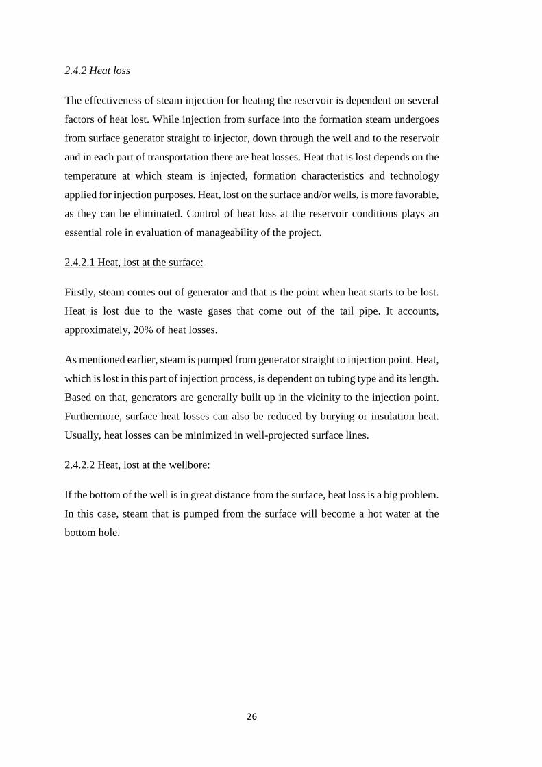
Figure 2.13. Heat loss in the wellbore in comparison with injection rate

(Farouq Ali, 1972)

As it can be noted in Figure 2.14, which illustrates the influence of steam injection rate

on bottom hole pressure, steam quality and heat loss, that in case of low injection rates,

heat losses are increasingly high, which gives a rise to reduced steam quality and

subsequently to increased pressure in the well. Generally, in case of small diameter

well, heat, lost in the wellbore, will be less than that of bigger diameter. As mentioned

earlier, heat losses are more or less dependent on rate of injection and depth. However,

it is also influenced by completion and casing types. In order not to lose a heat in the

wellbore, it is recommended to sustain it with insulation heat. Thus, considerable

amount of heat will contribute to heat the formation. (Satter A. 1965)

2.4.2.3 Heat, lost in the reservoir:

As indicated above, heat loss within the reservoir almost cannot be managed. Once

steam penetrated the formation, it starts to heat up upper and lower parts of the

reservoir. In this case, conduction plays an essential role in heat losses. As steam zone

becomes greater, the rate of heat loss also increases. This implies that the rate of heat

loss is influenced by the volume/area that steam is going to contact. Furthermore, the

rate of heat loss is also dependent on time. The rate of heat loss goes down once the

steam entered the reservoir and started to heat the rock.

28

Figure 2.14. Variation of heat losses to the formation with formation

thickness (Herbeck et.al. 1978)

In Figure 2.15 steam is injected at a constant rate of 1000 stb/d to the different

formation thicknesses. As it can be noted from the figure, the heat loss to the adjacent

formation rises with increase in steam zone area. Moreover, formation thickness and

heat loss to the reservoir are in counter-clock wise relationship with each other, which

implies that injection of steam to small areas will not be efficient. (Farouq Ali, 1974)

2.4.3 Types of steam injection:

Typically, there are two main types of steam injection: Cyclic steam injection and

continuous steam injection.

2.4.3.1. Cyclic steam injection:

It was noticed by Butler (1991) that cyclic steam injection is mainly used for

stimulation purposes, which leads to decrease in viscosity and cleaning of wellbore,

near wellbore area, thus, providing an additional energy for pushing oil towards

producing wells. In spite of the fact that oil production is less (only 10-25%) than that

for continuous steam injection, it is highly recommended and applied technique for

preliminary heating and preparing formation for application of further techniques.

Simplicity of this technique is based on the single-well pattern. First, the steam is

injected to the formation, then after a certain time injection is stopped for injected

steam to heat reservoir rock up, and finally the well is opened for producing the oil

(Figure 2.16). This technique is also called Huff and Puff method.

29

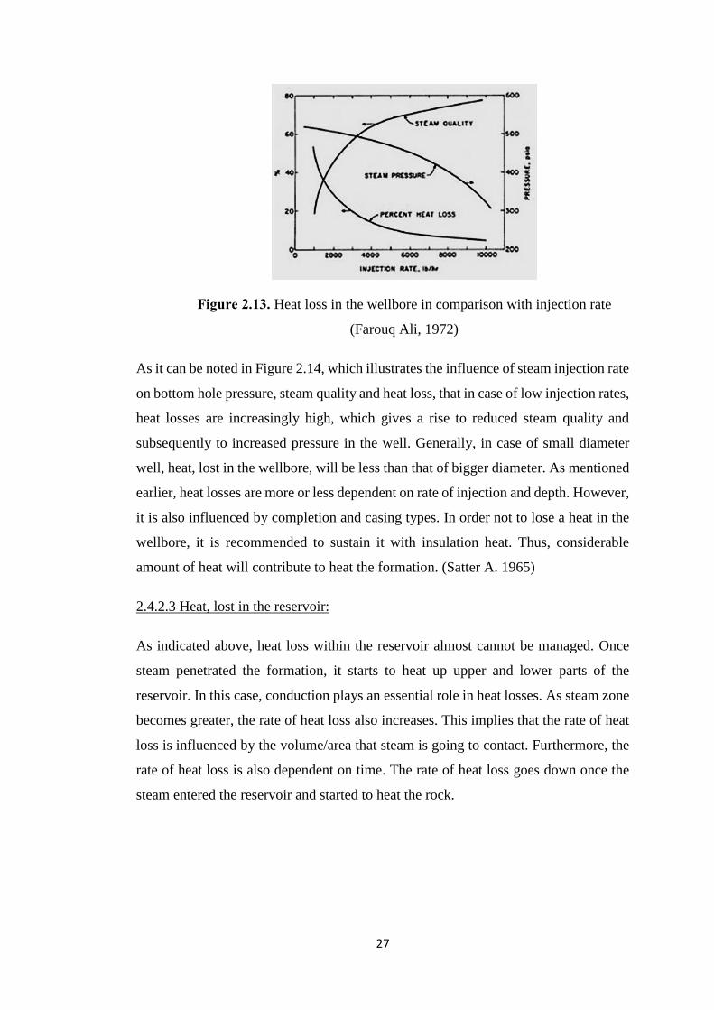
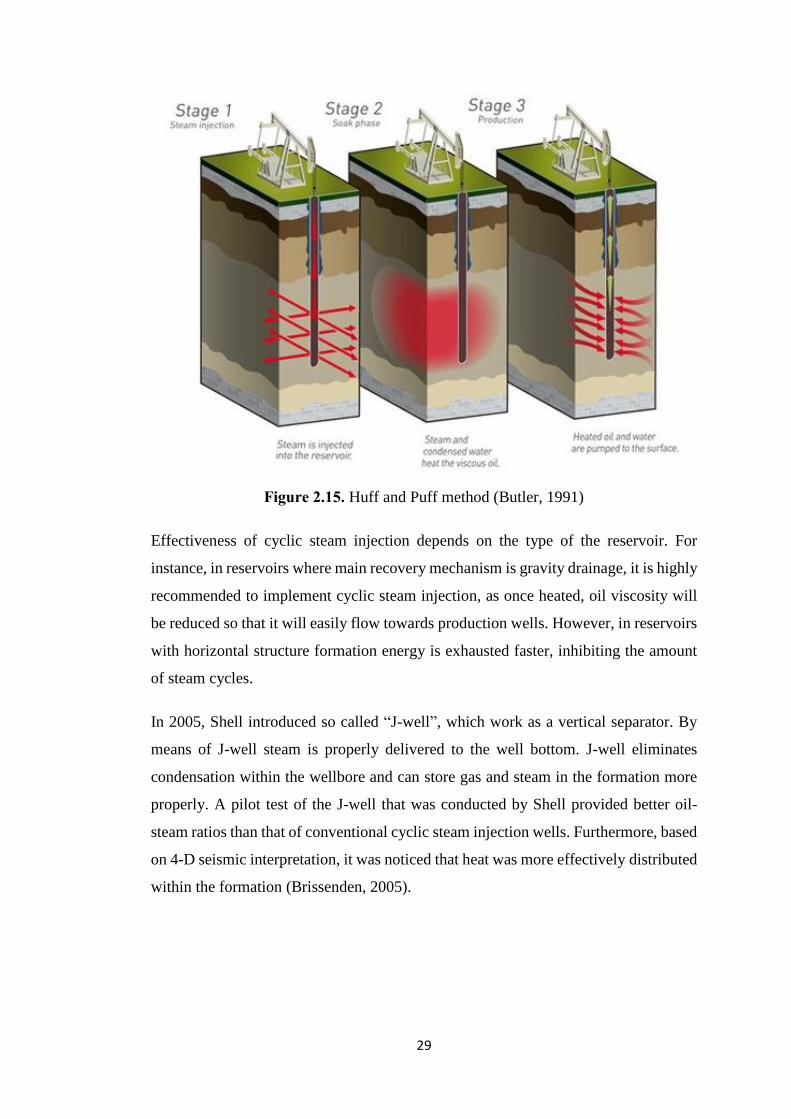
Figure 2.15. Huff and Puff method (Butler, 1991)

Effectiveness of cyclic steam injection depends on the type of the reservoir. For

instance, in reservoirs where main recovery mechanism is gravity drainage, it is highly

recommended to implement cyclic steam injection, as once heated, oil viscosity will

be reduced so that it will easily flow towards production wells. However, in reservoirs

with horizontal structure formation energy is exhausted faster, inhibiting the amount

of steam cycles.

In 2005, Shell introduced so called “J-well”, which work as a vertical separator. By

means of J-well steam is properly delivered to the well bottom. J-well eliminates

condensation within the wellbore and can store gas and steam in the formation more

properly. A pilot test of the J-well that was conducted by Shell provided better oil-

steam ratios than that of conventional cyclic steam injection wells. Furthermore, based

on 4-D seismic interpretation, it was noticed that heat was more effectively distributed

within the formation (Brissenden, 2005).

30

2.4.3.2. Continuous steam injection (CSI):

The procedure of continuous steam injection resembles that of water injection in

secondary recovery. The formation rock and oil are heated up by steam once it

penetrates reservoir. Heating process continues until steam condenses to the droplets.

As steam vapor reduces oil viscosity, it also provides gas drive to moveable oil. In the

formation the capacity of steam vapor is great. In other words, at 200 psi one barrel of

water produces 100 barrels of vapor (Farouq Ali., 1997). To recall, the viscosity of oil

can be reduced by 1000 times. In the reservoir steam starts to condense, thereby the

effective viscosity increases as well, bypassing the efficiency of steam and/or hot water

injection alone.

Generally, continuous steam injection technique increases recovery up to 50-60% of

OIP (Donaldson, 1989).

According to Das (2005) in case of bitumen reservoirs, conventional steam injection

is not sufficient to eliminate the problem of mobilization of bitumen, as it is almost

motionless in the formation due to API gravity. Due to immobile oil, the rates at which

steam should be injected would fracture the formation. Therefore, Steam Assisted

Gravity Drainage (SAGD) was evolved, for preventing the formation from fracturing

(Figure 2.17).

Figure 2.16. Steam Assisted Gravity Drainage. (Das, 2005)

31

The conceptual design of SAGD consists of a couple of horizontal wells for injection

and production. The main requirement of this technique is that injection well should

be over the producer, so that oil is heated up and moves down to production well by

gravity drainage.

The reason of implementation of SAGD for bitumen or immobile oils is that, these

play an important role in forming a steam chamber. Furthermore, vertical permeability

of the formation should be sufficient enough for heated and mobilized oil to flow down

to the production wells by gravity. For SAGD itself to be efficient, steam chamber

should be maintained with additional steam injection, which in turn will lead to

elimination of formation of liquid above the production well.

One of the first SAGD applications was conducted in the Alberta, for increasing

production in Tangleflags where oil viscosity was very high. It is a sandstone

formation with thickness about 13 meters, recovery from primary production of which

accounts for less than 1% of OIP (Thomas, 2008). Water coning played a negative role

in exploitation of the field.

Figure 2.17. SAGD technique in Tangleflags formation (Thomas, 2008)

As it can be seen from Figure 2.17, the injection well was drilled to the gas-oil contact,

for mobilization of oil, so that it can flow down to the production well. Favorable

pressure gradient towards producers played an essential role in lowering water coning.

(Jespersen et.al., 1993)

32

2.4.4 Selection Criteria

In spite of the fact that steam flood operation is an effective EOR technique, there are

some recommendations for implementation.

1) Formation with oil of lower viscosity and API gravity of which fluctuate around 10

to 20 API, are most suggested to be injected by steam.

2) As mentioned earlier, heat losses are lower for the formation which depth is less

than 3000 ft.

3) Rock permeability should be 500 md or higher for allowing viscous oil to flow.

4) From economical perspective oil content at 1200 bbl/acre-ft is beneficial

5) Rock thicknesses minimum should be 30-50 ft for inhibiting heat losses.

As noted above, for control of steam injection rate, lower reservoir pressures are more

favorable. On the other hand, in case of low reservoir pressure, the problems appear at

the production wells, as energy is not sufficient enough to lift oil to the surface.

Moreover, oil recovery will be low if steam temperature will be reduced, as in this case

oil viscosity will not be decreased sufficiently to flow. (Herbeck, E.F. et.al. 1978)

The main advantages of steam flood operations over other EOR techniques are: the

management of steam injection is easier than that of in situ burning. Oil is not cracked

in case of steam flooding, which implies that this technique ecologically is more

recommended. Furthermore, injection and production wells are not exposed to high

temperatures as in in-situ combustion.

2.4.5 Variations and optimization of steam flooding

2.4.5.1 Steam flooding prior to water injection:

By increasing the maturation by steam, oil recovery reduces. This is due to the fact

that steam-oil ratio (SOR) goes up to abnormally high numbers. Large SOR implies

that reservoir stores large volume of steam in the formation, while another portion of

it does not contribute to production.

33

At the end of 1980s it was recommended to change steam flood operation with water

injection. In this case the rearrangement of heat in the formation will take place, which

will lead to increase in recovery, as water will contribute to better oil sweep from areas

where steam left unswept. (Ault, J.W. 1985)

2.4.5.2 Water alternating steam:

The implementation of water alternating steam plays an important role for eliminating

or, at least, inhibiting steam breakthrough. This implies that, in case of Water

Alternating Steam injection sweep efficiency and oil production increase.

First application of this technique was effectively conducted in Russia from 1981 to

1984. Each year oil recovery has increased by 25-30%. Furthermore, implementation

Water Alternating Steam injection was also applied in California, which prevented

early steam breakthrough and increased oil production. (Hong, K.C. 1999)

2.4.5.3 Air injection after steam injection:

Sometimes it is beneficial to inject air after steam flood operations, as this scenario

may produce extra oil. British Petroleum experienced this first in Canada. After cyclic

steam stimulation, air was injected to the bitumen formation, located under Cold Lake.

Oil production increased by two times in comparison with single steam injection and

SOR decreased almost by three times from 6.1 to 2.3. (Hallam and Donnelly, 1988)

2.4.5.4 Hybrid Steam techniques:

In recent years, additives that are added to steam to accelerate the process of oil

production have captured the interest of petroleum industry. These additives may be

natural gas, CO2, flue gas, etc. The following processes may take place regarding

which catalyzer to add: viscosity reduction, decrease in residual oil saturation,

lowering interfacial tension, provides gas drive, etc.

From economical and ecological perspectives, co-injectants may lead to reduction in

amount of steam to be injected. In case of low amount of injected steam expenses,

emissions and usage of row materials will also be reduced.

34

Expanding Solvent Steam Assisted Gravity Drainage (ES SAGD) is a branch of SAGD

and consists of a combined injection of lighter hydrocarbons and steam together. In

this case, lighter hydrocarbons dilute in oil, thus reducing its viscosity. This process is

supported by steam, which heat rock and oil up. This technique has already been

applied with considerable increase in oil recovery, and decrease in SOR. Furthermore,

70% of the injected hydrocarbons could also be recovered after some period of time.

A pilot test in Liaohe oil field, which located in China, was conducted with the

combination of steam and flue gas injection. For diffusion and getting through the

formation the well was closed for 4 days. Once it was opened, better steam quality at

the bottom and decrease of SOR by 30% was obtained. (Zhu, C. Et.al. 2001)

2.4.5.5 Fracturing with Steam:

Experiences show that it is possible to recover petroleum from bitumen formations. In

case of the absence of gas cap and aquifer, cap rock acts as a barrier; therefore the

injection pressure may be increased to be higher than formation fracture pressure.

Consequently, mobilization of bitumen will take place. Fracturing would help to

recover bitumen from isolated areas. (Hong, 1999)

2.4.6 Steam injection implementation worldwide

The first implementation of cyclic steam injection (CSI) was in 1959 in Venezuela.

Production from the well where steam was injected was higher in comparison with

other ones. Afterwards, cyclic steam injection technique earned a big amount of

applications in Canada, Trinidad, China, USA etc. As mentioned earlier, steam

injection is best EOR technique for the fields with heavy oil. However, it took more

than 10 years for CSI technique to be modified and be more effective. In 1970s the

amount of steam injection cycles raised and in 1990 the number of stimulation cycles

increased to 39 in Mid-Way Sunset field, California. Moreover, 30 cycles were

counted by 75 wells, 20 cycles by 350 wells from the overall amount of 1500 (Jones

et.al., 1990). Clear image of steam and formation properties as well as conditions under

which steam is injected made it easier to increase the amount of cycles.

Development of horizontal wells also played an essential role in application of steam

injection technique. More precisely, Canada started application of screen sections in

35

horizontal wells in Cold Lake oil sands. Screen section in turn increases contact

between well and the formation.

Better optimization of pressure and temperature also led to the effectiveness of CSI

technique. For instance, in California in order to fracture the reservoir, steam was

injected at abnormally high pressures. Another example again is in California in

Midway-Sunset field, where successive steaming technique was implemented. The

purpose of this technique is to heat up the whole formation than individual well, so

that the whole reservoir would contribute to production. In such way, amount of oil

produced by each well increased by 30%.

Cold Lake field in Canada has undergone a lot of experiments and one of them is

Liquid Addition to Steam for Enhancing Recovery (LASER). In case of effectiveness

of this technique production can goes up by 3-6% of Oil Originally in Place. Table 2.4

illustrates oil recoveries of different thermal EOR techniques.

Table 2.4. Recovery of different thermal EOR processes. (Thomas, 2008)

Oil recovery factor

Thermal EOR % of OOIP

CSI 10-40

Steam flooding 50-60

SAGD 60-70

In-situ combustion 70-80

2.5 Modeling of CO2 injection and Steam injection

Starting from 70s, 80s EOR techniques started to be simulated for better understanding

of their impact.

2.5.1 Immiscible CO2 injection simulation

Immiscible CO2 injection project has been conducted in Turkey for the Bati Raman

Oilfield. Due to the existence of very little amount of dissolved gas within the

formation when CO2 started to be injected, only CO2 would flow in the reservoir. The

pressure required for development of miscibility is significantly higher than pressures

that can be reached in real life in the formation. Therefore, the operation is surely

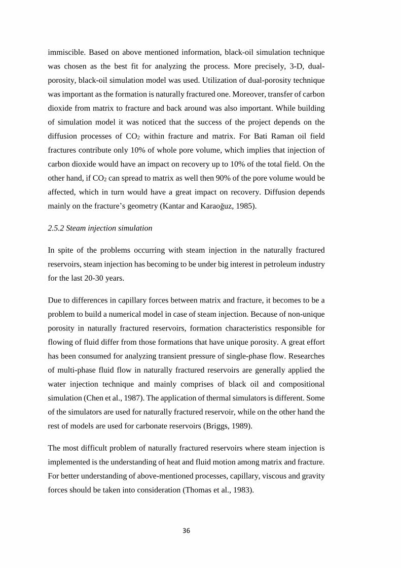
36

immiscible. Based on above mentioned information, black-oil simulation technique

was chosen as the best fit for analyzing the process. More precisely, 3-D, dual-

porosity, black-oil simulation model was used. Utilization of dual-porosity technique

was important as the formation is naturally fractured one. Moreover, transfer of carbon

dioxide from matrix to fracture and back around was also important. While building

of simulation model it was noticed that the success of the project depends on the

diffusion processes of CO2 within fracture and matrix. For Bati Raman oil field

fractures contribute only 10% of whole pore volume, which implies that injection of

carbon dioxide would have an impact on recovery up to 10% of the total field. On the

other hand, if CO2 can spread to matrix as well then 90% of the pore volume would be

affected, which in turn would have a great impact on recovery. Diffusion depends

mainly on the fracture’s geometry (Kantar and Karaoğuz, 1985).

2.5.2 Steam injection simulation

In spite of the problems occurring with steam injection in the naturally fractured

reservoirs, steam injection has becoming to be under big interest in petroleum industry

for the last 20-30 years.

Due to differences in capillary forces between matrix and fracture, it becomes to be a

problem to build a numerical model in case of steam injection. Because of non-unique

porosity in naturally fractured reservoirs, formation characteristics responsible for

flowing of fluid differ from those formations that have unique porosity. A great effort

has been consumed for analyzing transient pressure of single-phase flow. Researches

of multi-phase fluid flow in naturally fractured reservoirs are generally applied the

water injection technique and mainly comprises of black oil and compositional

simulation (Chen et al., 1987). The application of thermal simulators is different. Some

of the simulators are used for naturally fractured reservoir, while on the other hand the

rest of models are used for carbonate reservoirs (Briggs, 1989).

The most difficult problem of naturally fractured reservoirs where steam injection is

implemented is the understanding of heat and fluid motion among matrix and fracture.

For better understanding of above-mentioned processes, capillary, viscous and gravity

forces should be taken into consideration (Thomas et al., 1983).

37

After some investigations several steam injection modeling techniques were proposed.

One of them implies that the thermal dual-porosity within dual-permeability

simulation model has to be built to eliminate the problems. The model itself is built in

3-D format, and includes formation heterogeneities. The design of producers and

injectors is multi-layer and wells are connected to the reservoir fully implicitly (Dean

and Lo, 1988).

38

39

CHAPTER 3

STATEMENT OF THE PROBLEM

Throughout last decades a considerable amount of studies and work are concentrated

on development of technology, software, etc. to increase production from heavy oil

reservoirs. Enhanced oil recovery techniques proved to be an efficient alternative after

primary and secondary recoveries. Additional investments are made to increase

recovery factor of EOR techniques. Thus, considerable development took place in

injection of carbon dioxide and in steam injection operations.

The selection of most convenient EOR technique to apply for an oil field is a

challenging process. This study is generated based on production scenarios appropriate

for heavy oil field by using geological modeling software (Schlumberger’s Petrel).

Although, the geological model accounts only the basic (such as: porosity,

permeability, API gravity) parameters of heavy oil field, it can be used to evaluate

different scenarios of enhanced oil recovery techniques. Several scenarios are

constructed, such as: continuing the water injection, steam injection without CO2

injection, CO2 injection, etc.

A reservoir model is generated and run using Schlumberger’s Eclipse simulator in

order to understand the effect of CO2 injection prior to steam injection. The

comparison of recovery performances at different cases helps us to understand the

most effective path of applying enhanced oil recovery techniques.

40

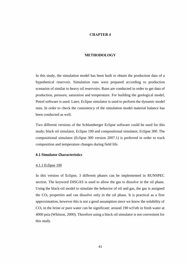
41

CHAPTER 4

METHODOLOGY

In this study, the simulation model has been built to obtain the production data of a

hypothetical reservoir. Simulation runs were prepared according to production

scenarios of similar to heavy oil reservoirs. Runs are conducted in order to get data of

production, pressure, saturation and temperature. For building the geological model,

Petrel software is used. Later, Eclipse simulator is used to perform the dynamic model

runs. In order to check the consistency of the simulation model material balance has

been conducted as well.

Two different versions of the Schlumberger Eclipse software could be used for this

study; black oil simulator, Eclipse 100 and compositional simulator, Eclipse 300. The

compositional simulator (Eclipse 300 version 2007.1) is preferred in order to track

composition and temperature changes during field life.

4.1 Simulator Characteristics

4.1.1 Eclipse 100

In this version of Eclipse, 3 different phases can be implemented in RUNSPEC

section. The keyword DISGAS is used to allow the gas to dissolve in the oil phase.

Using the black-oil model to simulate the behavior of oil and gas, the gas is assigned

the CO2 properties and can dissolve only in the oil phase. It is practical as a first

approximation, however this is not a good assumption since we know the solubility of

CO2 in the brine or pure water can be significant: around 190 scf/stb in fresh water at

4000 psia (Whitson, 2000). Therefore using a black oil simulator is not convenient for

this study.

42

4.1.2 Eclipse 300

This version of Eclipse, allowing a compositional model is more accurate for this

study. The oil phase is represented by hydrocarbon components and carbon dioxide is

introduced as another component. The simulation model contains also water. The

solubility of the gas in the aquifer is taken into account. In the RUNSPEC section the

CO2SOL option illustrate this possibility. Regarding the computation method, it uses

the fully implicit method, so that at every time step the pressure dependent terms (such

as; density, gas formation volume factor, or viscosity) are evaluated. Peng-Robinson

equation of state method is used.

The GRID section comprises physical parameters for the grid blocks, and also

keywords as AQUNUM to assign a numerical aquifer to a grid block and AQUCON

to specify the connection data for numerical aquifers are used to simulate an aquifer

in a grid block.

Table 4.1. Main parameters

Parameter Value

Porosity 17%

Absolute Permeability 50 mD

Depth at the top 4300 feet

Transmissibility 1

The PROPS section sums up the CO2 properties described earlier, the water and oil

relative permeability values are added. The residual oil saturations have been defined

so that 20% oil remains after the waterflood and 5% oil after the CO2-flood.

4.2 Model Setup

Geological model has been built using Petrel software based on a similar anticlinal

structure of the Bati-Raman oil field. The model area divided into 3283 elements (67

rows and 49 columns) using regular structured grids with the size of each element is

640 ft by 670 ft (Figure 4.1). The outer boundaries of the model are no-flow

boundaries. The model defines a system made up of 20 sub layers. Net to gross (NTG)

variation is around 0.38-0.45. Average permeability is around: 40-50 mD. Porosity is

43

around 0.18-0.2. There is no any standard PVT correlation in Eclipse which can be

used for heavy oil API<15, therefore heavy oil PVT was calculated based on De Ghetto

at al. (1995) correlation, which contains modified PVT correlations for estimating

bubble point pressure, solution gas oil ratio (RS), oil formation volume factor (BO), oil

compressibility (co) and oil viscosity (μo) for the heavy oil (10<API<22.3). For

developing this correlation fluid samples were taken from the Mediterranean Basin,

Africa, and the Persian Gulf. When comparing published correlations, De Ghetto et al.

(1995) decided that the Vasquez and Beggs correlation estimated the oil formation

volume factor with minimal error, and therefore no further modification was needed.

Compared to other correlations, pressure and temperature at the separator is mandatory

in the De Ghetto et al. (1995) correlation. Eclipse 300 Thermal solution type has been

used as “Fully Implicit”.

The model consists of total pore volume of 78 MM rb (total fluid volume) and

hydrocarbon pore volume (HCPV) of approximately 63 MM rb with initial average oil

saturation of 0.8. The reservoir depth is taken to be 4300 ft with one injection well and

four production wells. Well bore diameter is taken as 0.375 ft and wells are produced

using minimum bottom hole flowing pressure control mode. Injection pressure is set

to be 1900 and 100 psia is specified for production wells as pressure constraints. The

simulation is run for 54 years from 1962 to 2016.

Figure 4.1. Grid model

44

Corey relative permeability functions were used with residual water saturation set at

0.3, and residual gas saturation as 0.05, while capillary effects were not taken into

account. The diffusion coefficients of methane and CO2 were taken as follows: 10-5

m2/s in the gas phase, 1.5-2.1·10−9 m2/s in the aqueous phase. Figures 4.2, 4.3, and 4.4

show the relative permeability curves for oil, gas and water phases, respectively.

Capillary pressure is neglected for simplicity, but it should be emphasized that core

data treatment to determine both relative permeability and capillary pressure is an

important issue, and of particular interest for long term behavior, and fluid propagation

after the injection phase. Rock compressibility is 5×10-4 1/psi. Reference pressure is

set as 1800 psia. Rock thermal conductivity is around 24 Btu/ft·day·°F.

Figure 4.2 Oil relative permeability

Figure 4.3. Water relative permeability

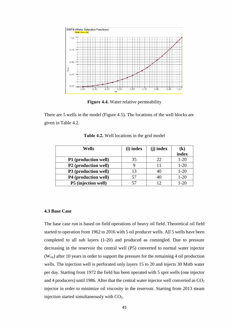
45

Figure 4.4. Water relative permeability

There are 5 wells in the model (Figure 4.5). The locations of the well blocks are

given in Table 4.2.

Table 4.2. Well locations in the grid model

Wells (i) index (j) index (k)

index

P1 (production well) 35 22 1-20

P2 (production well) 9 11 1-20

P3 (production well) 13 40 1-20

P4 (production well) 57 40 1-20

P5 (injection well) 57 12 1-20

4.3 Base Case

The base case run is based on field operations of heavy oil field. Theoretical oil field

started to operation from 1962 to 2016 with 5 oil producer wells. All 5 wells have been

completed to all sub layers (1-20) and produced as comingled. Due to pressure

decreasing in the reservoir the central well (P5) converted to normal water injector

(Winj) after 10 years in order to support the pressure for the remaining 4 oil production

wells. The injection well is perforated only layers 15 to 20 and injects 30 Mstb water

per day. Starting from 1972 the field has been operated with 5 spot wells (one injector

and 4 producers) until 1986. After that the central water injector well converted as CO2

injector in order to minimize oil viscosity in the reservoir. Starting from 2013 steam

injection started simultaneously with CO2.

46

Figure 4.5. All well are producers

Figure 4.6. Central well is converted to CO2/Steam injection well

The impact of implemented EOR techniques by the following scenarios can be

understood and visualized better by comparing with the base case.

4.4 Scenarios

Simulation model has been run at 6 various scenarios to understand the impacts and

efficiency of EOR techniques, specifically the effect of CO2 injection prior to the

steam injection.

47

4.4.1 Scenario 1:

In this scenario, field started to operation from 1962 with 5 producers without any

pressure support (primary production). At the beginning of 1971, central well

converted to normal water injector until 2016.

4.4.2 Scenario 2:

In this scenario, simulation model has been run as 5 spot injection of CO2 from the

central well after a primary production phase between 1962 and 1971. CO2 injection

started at 1 January 1971 and continued until 2016.

4.4.3 Scenario 3:

In this scenario steam is injected starting from 1971 without any prior water injection.

During 1962 to 1971, all 5 wells are used for production. The steam injection

continued until 2016.

4.4.4 Scenario 4:

This case covered steam and immiscible CO2 injection simultaneously from starting

at the same injection time on 1971. Although it is difficult to implement simultaneous

CO2 and steam injection from the same well in real situations, it is aimed to see the

effect on the recovery. The primary recovery takes place between 1962 and 1971 as

before and the injection ends on 2016.

4.4.5 Scenario 5:

In this scenario the options of immiscible CO2 flooding followed by steam injection is

analyzed. Following the primary recovery between 1962 and 1971, CO2 is injected

from the central well until 1986, then it is replaced by a steam injector and run has

finished on 2016. The difference between this scenario and the base case is the lack of

water injection in this case.

4.4.6 Scenario 6:

In this case, water flooding (1971 to 1986) instead of CO2 injection is implemented

before the steam injection starting after the primary recovery period of 1962 to 1971.

48

The steam injection takes place between 1986 and 2016. The comparison of this

scenario with the Scenario 5 shows the effect of water injection and CO2 injection prior

to steam injection.

4.4.7 Scenario 7:

In this scenario water injection started in 1971, immediately after primary production

stage. The difference of this scenario with scenario 1 is that for this case water was

injected to all 20 zones.

4.4.8 Scenario 8:

This scenario represents the same water injection technique, which started in 1971.

The main difference is that the distance of producing wells was reduced ( 2 km towards

injection well)

4.5 Material Balance

Nowadays, there is a belief that numerical simulation modeling technique is more

advantageous over material balance concept that has been used in oil industry.

However, usage of the numerical simulation techniques together with the material

balance concept would reduce the risk of errors that are hard to identify when using

numerical techniques alone.

In order to identify the average pressure decline trend, material balance can be used

with only production and pressure histories and with awareness of fluid PVT

properties. Thus, no geological models are required in case of material balance, which

calculates STOIIP and identify reservoir drive mechanism. Therefore, it is the easiest

and fastest technique in oil industry since it is the minimum assumption route through

the subject of reservoir engineering.

Material balance and simulation modeling are not competitors at all. Conversely, they

should be used in supportive purposes of one another: material balance defines the

system and transported to the simulation model as an input. As a matter of fact,

material balance is a powerful tool in applying for history matching production

performance, nevertheless, prediction is the disadvantage of this technique. Therefore,

for prediction simulation modeling technique should be used.

49

A material balance evaluation tool is used to compare the pressure data obtained from

the simulation run. Material Balance evaluation is done in Integrated Production

Modeling software (IPM), called MBal. The tool uses analytical techniques for

investigation of fluid dynamics of the field, basic principle of which is classical

material balance equation. It is possible to obtain a realistic profiles by means of MBal

with or without history matching. (IPM Products. 2010)

50

51

CHAPTER 5

RESULTS AND DISCUSSIONS

5.1 Base Case

Simulation model has been built and computed using the THERMAL option of the

Eclipse 300 simulator. The cases applied in the study are summarized in Table 5.1.

Figure 5.1 shows daily oil production and cumulative oil production obtained using

the base case. In the Base case all 5 wells produce heavy oil without any pressure

support and stimulation. Those wells penetrated and completed for each zone. Well

control has been set to minimum flowing bottom hole pressure (BHFP) of 100 psia for

each well.

Table 5.1. The summary of the simulation cases

Case Primary

production

Water

injection

CO2

injection

Steam

injection

Base case 1962 - 1971 1971- 1986 1986 - 2013 2013 - 2016

Scenario 1 1962 - 1971 1971 - 2016 - -

Scenario 2 1962 -1971 - 1971 - 2016 -

Scenario 3 1962 - 1971 - - 1971 - 2016

Scenario 4 1962 - 1971 - 1971 - 2016 1971 - 2016

Scenario 5 1962 - 1971 - 1971 - 1986 1986 – 2016

Scenario 6 1962 - 1971 1971 - 1986 - 1986 - 2016

52

Figure 5.1 Field daily oil production rate

Figure 5.1 shows the quick rate decrease in production wells is followed by a short

recovery period. Then the rate continues to decrease until end of primary production

period. The decline in production rate is slowed down with the start of water injection

on 1971. The sharp decrease seen on rate in 1971 is because of the conversion of one

of the producers to an injector. Starting to inject CO2 on 1986 has a negative effect on

the production rate as seen from the changing trend of the rate.

Figure 5.2 Average reservoir pressures

Two different permeability values have been used to understand the effect of

permeability on the reservoir pressure. Figure 5.2 shows average reservoir pressure

based on 50 mD and 100 mD. Higher permeability caused the waterflooding period

(between 1971 and 1986) to be more effective comparing the lower permeability case.

Similarly the steam injection at the end of the run shows an increase in the reservoir

0

1000000

2000000

3000000

4000000

5000000

6000000

7000000

8000000

0

200

400

600

800

1000

1200

1962 1975 1989 2003 2016

Oil,

stb

/d

Field Oil Production, stb/d

Daily Oil Rate, stb/d Cumulative Oil Production, stb

0

500

1000

1500

2000

1962 1975 1989 2003 2016

Pre

s,

psia

Average Reservoir Pressure, psia

Average Reservoir Pressure (100mD)

Average Reservoir Pressure (50mD)

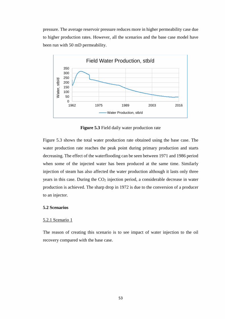
53

pressure. The average reservoir pressure reduces more in higher permeability case due

to higher production rates. However, all the scenarios and the base case model have

been run with 50 mD permeability.

Figure 5.3 Field daily water production rate

Figure 5.3 shows the total water production rate obtained using the base case. The

water production rate reaches the peak point during primary production and starts

decreasing. The effect of the waterflooding can be seen between 1971 and 1986 period

when some of the injected water has been produced at the same time. Similarly

injection of steam has also affected the water production although it lasts only three

years in this case. During the CO2 injection period, a considerable decrease in water

production is achieved. The sharp drop in 1972 is due to the conversion of a producer

to an injector.

5.2 Scenarios

5.2.1 Scenario 1

The reason of creating this scenario is to see impact of water injection to the oil

recovery compared with the base case.

0

50

100

150

200

250

300

350

1962 1975 1989 2003 2016

Wate

r, s

tb/d

Field Water Production, stb/d

Water Production, stb/d

54

Figure 5.4. Comparison of base case and scenario-1 average reservoir pressure

Figure 5.5. Comparison of base case and scenario-1 oil production rates

Figure 5.4 shows that water injection supports the reservoir pressure. The effect of this

pressure support can be seen on the oil production rate as well (Figure 5.5). On the

other hand, Figure 5.6 shows the high water production rates due to water flooding.

0

500

1000

1500

2000

1962 1975 1989 2003 2016

Pre

ssu

re, p

sia

Average Reservoir Pressure, psia

Base Case(50mD)

Case1

0

200

400

600

800

1000

1200

1962 1975 1989 2003 2016

Oil,

stb

/d

Field Oil Production Rate, stb/d

Base Case

Case1

55

Figure 5.6. Comparison of base case and scenario-1 water production rates

5.2.2 Scenario 2

In this scenario the effect of the CO2 injection can be observed. Figure 5.7 shows the

drop in reservoir pressure in 1971 when the CO2 injection starts. Comparing to water

flooding, CO2 injection is less effective in supporting the pressure in the reservoir. As

CO2 injection is immiscible, it acts like a simple gas injection technique by gathering

at the top as a gas cap.

Figure 5.7. Comparison of base case and scenario-2 average reservoir pressure

Figure 5.8 shows the decrease in the production rate during CO2 injection period.

0

100

200

300

400

1962 1975 1989 2003 2016

Wa

ter,

stb

/d

Field Water Production, stb/d

Base Case

Case1

0

500

1000

1500

2000

1962 1975 1989 2003 2016

Pre

ssu

re, p

sia

Average Reservoir Pressure, psia

Base Case(50mD)

Case2

56

Figure 5.8. Comparison of base case and scenario-2 oil production rates

5.2.3 Scenario 3

In this scenario steam is injected to the all layers to increase the oil mobility by

minimizing its viscosity between 1971 and 2016.

Figure 5.9. Comparison of base case and scenario-3 average reservoir pressure

The pressure, oil production and water production responses of the field to steam

injection after 1971 are very similar as seen from Figure 5.9, Figure 5.10 and Figure

5.11. In the long run, steam injection becomes more effective comparing to water

injection.

0

200

400

600

800

1000

1200

1962 1975 1989 2003 2016

Oil,

stb

/d

Field Oil Production, stb/d

Base Case

Case2

0

500

1000

1500

2000

1962 1975 1989 2003 2016

Pre

ssu

re, p

sia

Average Reservoir Pressure, psia

Base Case(50mD)

Case3

57

Figure 5.10. Comparison of base case and scenario-3 oil production rates

Figure 5.11. Comparison of base case and scenario-3 water production rates

5.2.4 Scenario 4

This case covers steam and CO2 injection from starting at the same injection time as

in scenario 3. Actually the purpose of running this combination case is to identify

which EOR method has more benefit for this field during various life of field. In spite

of the fact that in real life it would be hard to implement such a technique, in Eclipse

there is such a function that allows the injection of CO2 and steam at the same time

from the same well.

Figure 5.12 shows that steam injection combined with CO2 injection is almost equal

to steam injection case (scenario-3).

0

200

400

600

800

1000

1200

1962 1975 1989 2003 2016

Oil,

stb

/d

Field Oil Production, stb/d

Base CaseCase3

0

100

200

300

400

1962 1975 1989 2003 2016

Wa

ter,

stb

/d

Field Water Production, stb/d

Base Case

Case3

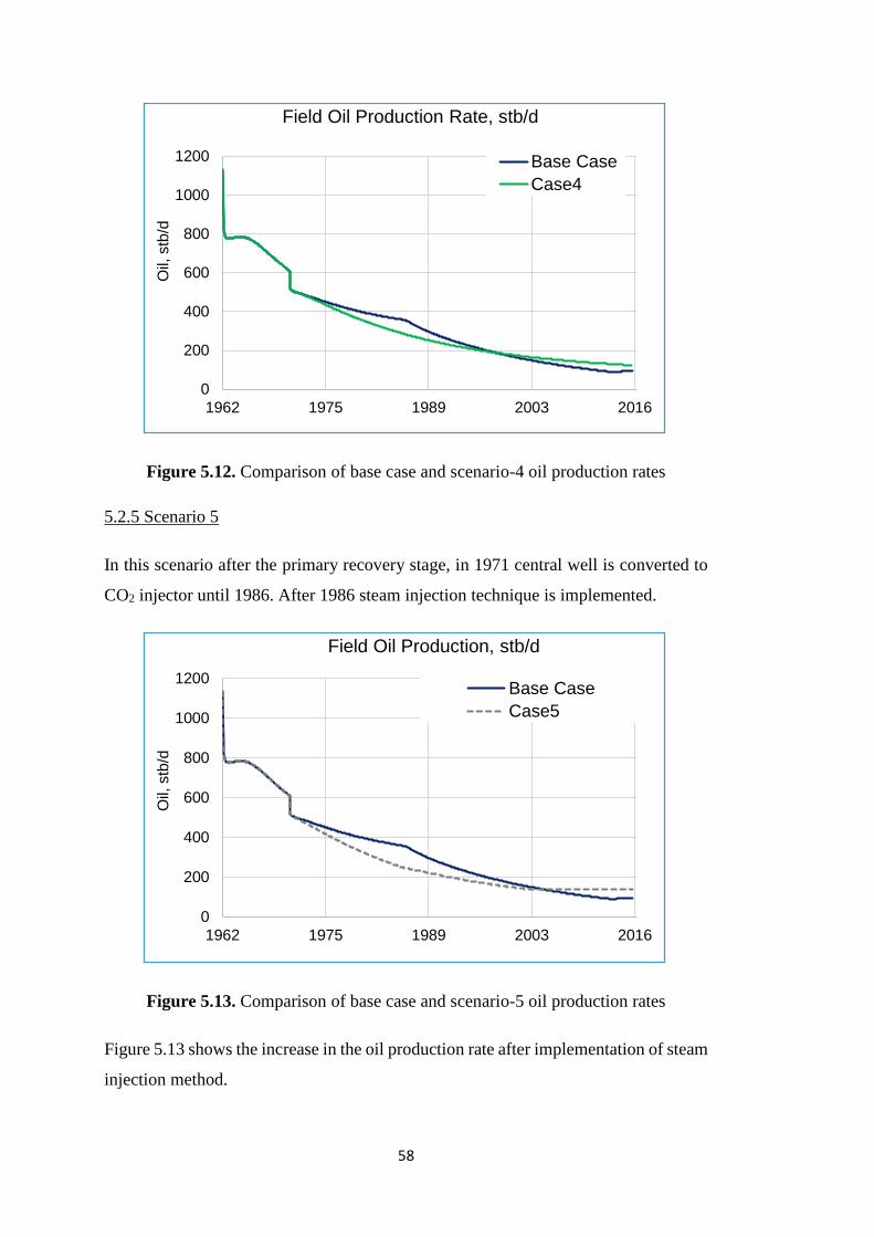
58

Figure 5.12. Comparison of base case and scenario-4 oil production rates

5.2.5 Scenario 5

In this scenario after the primary recovery stage, in 1971 central well is converted to

CO2 injector until 1986. After 1986 steam injection technique is implemented.

Figure 5.13. Comparison of base case and scenario-5 oil production rates

Figure 5.13 shows the increase in the oil production rate after implementation of steam

injection method.

0

200

400

600

800

1000

1200

1962 1975 1989 2003 2016

Oil,

stb

/d

Field Oil Production Rate, stb/d

Base Case

Case4

0

200

400

600

800

1000

1200

1962 1975 1989 2003 2016

Oil,

stb

/d

Field Oil Production, stb/d

Base Case

Case5

59

5.2.6 Scenario 6

In this scenario primary recovery stage starts in 1962 and lasts until 1971 when central

well is converted to water injection well. From 1986 onwards steam injection

technique is implemented in the field.

Figure 5.14. Comparison of base case and scenario-6 oil production rates

Figure 5.14 shows the improvement in oil production rate due to steam injection. CO2

is injected in base case starting from 1986 instead of steam.

5.3 Comparison of all Scenarios

If the pressure responses of all the cases are compared, it can be seen from Figure 5.15

that scenario-1 is the most effective one in terms of supporting reservoir pressure. In

scenario-1 water injection keeps the pressure level high.

0

200

400

600

800

1000

1200

1962 1975 1989 2003 2016

Oil,

stb

/d

Field Oil Production, stb/d

Base CaseCase6

60

Figure 5.15 Comparison of field average reservoir pressure

Table 5.2. Oil production rates

Year Base

Case

Scenario

1

Scenario

2

Scenario

3

Scenario

4

Scenario

5

Scenari

o 6

1962 776 776 776 776 776 776 776

1970 607 607 607 607 607 607 607

1971 514 514 514 514 514 514 514

1980 394 394 322 348 350 326 394

1990 273 333 196 235 239 212 289

2000 165 303 121 169 175 148 291

2010 102 287 75 130 137 138 283

2015 94 283 60 117 125 139 280

Oil production rates are given in Table 5.2 and in Figure 5.16.

The comparison of oil production rates show that scenarios 2, 3 and 4 represent

intermediate options. From Figure 5.16 it can be noted that scenario 2 (CO2 injection)

is the least efficient technique, compared to scenarios 3 (steam injection) and scenario

4 (steam + CO2 injection). However, the impact of scenarios 3 and 4 to the reservoir

pressure is slightly different (better for scenario 4). On the other hand from economical

perspectives comingled injection of steam/CO2 would require more financial

contribution to the project, with slight impact of pressure support. Therefore

comparing scenarios 2, 3, and 4; the best solution is to implement steam injection

technique.

0

500

1000

1500

2000

1962 1975 1989 2003 2016

Pre

s, p

sia

Average Reservoir Pressure, psia

61

Figure 5.16 Comparison of field oil production rates

As it can be noted from Figure 5.15 and Figure 5.16, the trendline of scenario 5 is the

same with that of scenario 2. However after 1986, due to the implementation of steam

flood operation, pressure started to increase. By the end of time schedule reservoir

pressure even overpasses scenarios 2, 3, and 4 as well as the base case. Outcome of

scenario 5 clearly demonstrates that steam flood technique should be implemented in

the field as early as possible in terms of reservoir pressure support.

In scenario 6 immediately after primary recovery stage, water injection technique is

implemented in the field. Therefore the trendline is the same as that of the scenario 1.

However, after 1986 water injection is replaced by steam injection. If we compare base

case and scenarios 1 and 6 we can clearly find out that until 1986 all three follow the

same trendline. Afterwards reservoir pressure for the base case declines too fast as

carbon dioxide is injected to the reservoir. It can be noted from scenarios 1 and 6 that

pressure response for scenario 1 is much better which may be due to the fact that water

spreads throughout the reservoir more uniformly. On the other hand it can be noted

that steam injection implementation has a long-term goal, because it takes more time

for steam to heat up the oil and mobilize it. Therefore, after 2010 reservoir pressure

even started to increase as steam injection heat oil up as well as has an impact in

additional drive.

0

200

400

600

800

1000

1200

1962 1975 1989 2003 2016

Oil,

stb

/d

Field Oil Production, stb/d

Base Case Case1

Case2 Case3

Case4 Case5

Case6

62

Cumulative oil production for scenario 1 is around 8 Mstb which is 2 Mstb higher than

that of base case. However, it should be mentioned that techniques implemented for

base case, was conducted properly. So that the cumulative oil production of the base

case represents the highest trend compared to scenarios 2, 3, and 4.

Figure 5.17 Comparison of cumulative oil production

Based on pressure responses and cumulative oil production seen in Figure 5.17, among

the applied techniques it would obviously be recommended to implement scenario 1

or scenario 6 to the field.

Figure 5.18 Comparison of water production rate

0

2,000

4,000

6,000

8,000

10,000

1962 1975 1989 2003 2016

Oil,

Mstb

Field Oil Production, Mstb/d

Base Case Case1

Case2 Case3

Case4 Case5

Case6

0

100

200

300

400

1962 1975 1989 2003 2016

Wa

ter,

stb

/d

Field Water Production, stb/d

Base Case Case1

Case2 Case3

Case4 Case5

Case6

63

Figure 5.18 shows field water production rate. The highest water production is in

scenario 1. The reason of such huge water amount is due to the fact that in scenario 1,

water injection well is online until the end of time schedule. For cases 5 and 6, the

steam injection technique is implemented from 1986 and water production starts to

decrease. However, once steam is condensed to droplets, water production starts to

increase which can be seen after 2008. The lowest water production is in scenario 2,

which is CO2 injection technique.

Figure 5.19 and Figure 5.20 show the temperature distribution for scenario-6 on

September 1963 and June 2016, respectively. As it can be noted, at the beginning of

the production, when all wells are producers, the temperature starts to decrease in near

wellbore areas due to pressure decrease, with outer boundaries remain at high

temperatures. By the end of time schedule, temperatures at producers are minimum,

while central, injection well has the highest temperature as steam is injected.

Figure 5.19 Reservoir temperature distribution for scenario-6 on September 1963

64

Figure 5.20 Reservoir temperature distribution for scenario-6 on June 2016

Figure 5.21 shows the pressure changes within the reservoir in scenario-6. As it can

be noted, at the onset of production pressure response can only be seen at near wellbore

areas (Figure 5.21, a). Once water started to be injected, pressure started to be

supported as considerable pressure reductions are found only in near wellbore areas of

producing well (Figure 5.21, b). As more and more oil is produced from the field, the

whole picture does not change. The only difference is that further areas started to

influence to production as they are drained and pressure decrease can be seen there.

(Figure 5.21, c and d)

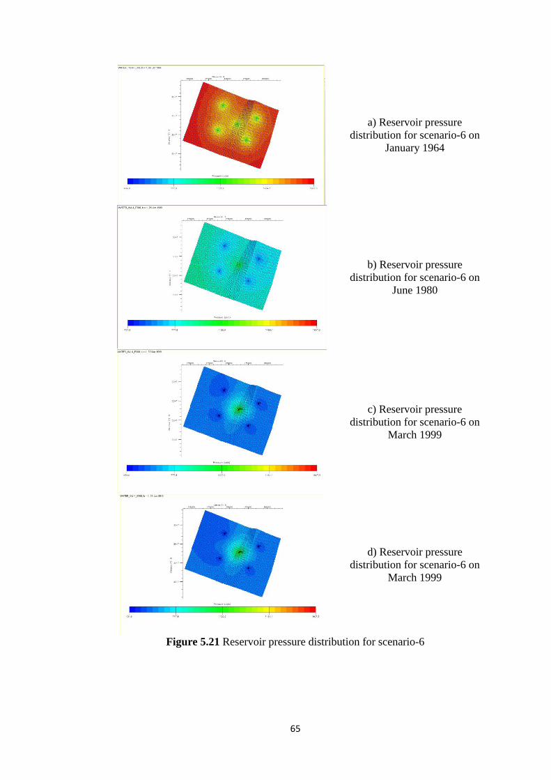
65

a) Reservoir pressure

distribution for scenario-6 on

January 1964

b) Reservoir pressure

distribution for scenario-6 on

June 1980

c) Reservoir pressure

distribution for scenario-6 on

March 1999

d) Reservoir pressure

distribution for scenario-6 on

March 1999

Figure 5.21 Reservoir pressure distribution for scenario-6

66

Figure 5.22 Viscosity distribution for scenario 6

Figure 5.22 shows viscosity changes within the reservoir in scenario-6. As it can be

noted, at the onset of production viscosity reduction can only be seen at near wellbore

areas and the reduction is not big, as reservoir contains a viscous oil (Figure 5.22, a).

After water injection and 4 years of steam flooding it can be noted that viscosity

a) Viscosity distribution

for scenario 6 in 1963

b) Viscosity distribution

for scenario 6 in 1990

c) Viscosity distribution

for scenario 6 in 1997

d) Viscosity distribution

for scenario 6 in 2016

67

reduction distribution is higher in the right hind-side of the figure (figure 5.22 b). As

more steam is injected to the field, the whole picture of viscosity reduction does not

change so far. The only difference is that viscosity has reduced in further areas further

areas started to influence to production as they are drained and pressure decrease can

be seen there. (Figure 5.21, c and d)

5.4 Effect of CO2 on steam injection

The effect of CO2 injection on recovery from steam injection can be compered using

scenario 5 (CO2 injection followed by steam injection) and scenario 6 (water injection

followed by steam injection).

Figure 5.23 Effect of water injection and CO2 injection before steam injection on oil

production rates

0

200

400

600

800

1000

1200

1962 1975 1989 2003 2016

Oil,

stb

/d

Field Oil Production, stb/d

Case5 Case6

68

Figure 5.24 Effect of water injection and CO2 injection before steam injection on

cumulative oil production

The water injection between 1971 and 1986 has increased the production rate

comparing to CO2 injection. Therefore it is not easy to see the effect of water injection

or CO2 injection on recovery by steam injection on Figures 5.23 and 5.24. However

the cumulative oil production can be compared between 1986 and 2016. Additional

cumulative oil production following water injection is 4716 Mstb. During the same

period additional oil recovery becomes 1828 Mstb by steam injection followed by CO2

injection. This shows that it is better to apply steam injection after water injection

rather than CO2 injection. The reason of this behavior can be based on the fact that

water has a greater latent heat comparing to CO2. Therefore although heating the

reservoir saturated by water is more difficult, it also takes more time to cool down.

5.5 Effect of Water Injection Wells

In order to understand the effect of water injection wells’ position and completion

interval on oil and water production two additional runs have been performed. The

water injection well has been completed in all layers instead of 5 layers in the first

case. In the second case the production wells are located closer to the injection well

(Figure 5.25). The new scenarios are summarized in Table 5.3.

0

1,000

2,000

3,000

4,000

5,000

6,000

7,000

8,000

1962 1975 1989 2003 2016

Oil,

Mstb

Field Oil Production, Mstb/d

Case5

Case6

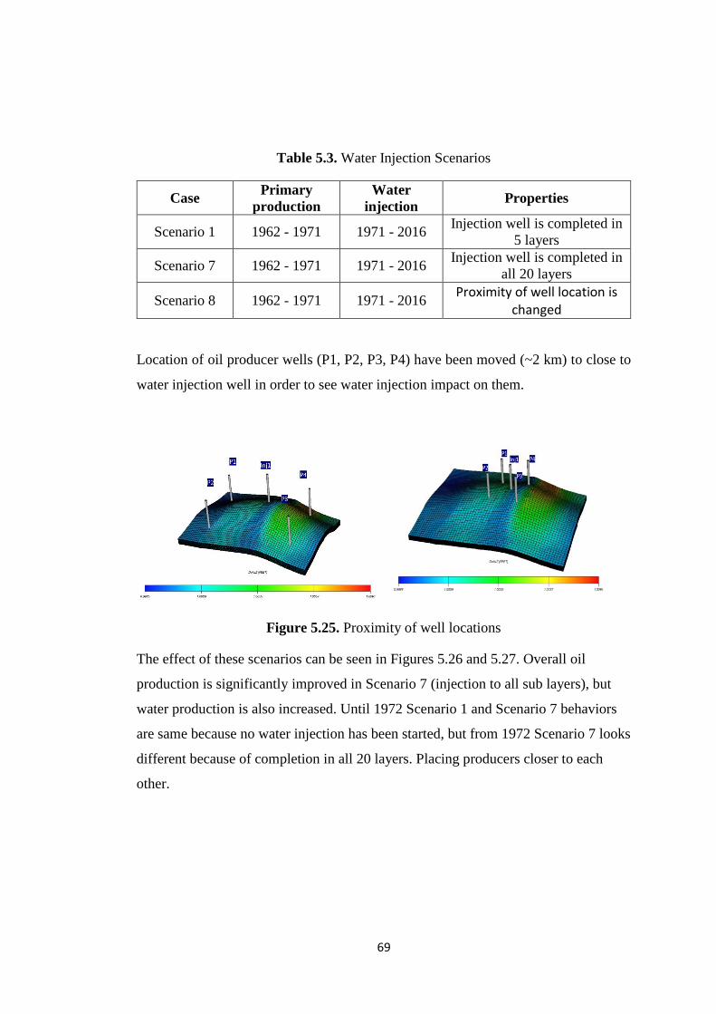
69

Table 5.3. Water Injection Scenarios

Case Primary

production

Water

injection Properties

Scenario 1 1962 - 1971 1971 - 2016 Injection well is completed in

5 layers

Scenario 7 1962 - 1971 1971 - 2016 Injection well is completed in

all 20 layers

Scenario 8 1962 - 1971 1971 - 2016 Proximity of well location is

changed

Location of oil producer wells (P1, P2, P3, P4) have been moved (~2 km) to close to

water injection well in order to see water injection impact on them.

Figure 5.25. Proximity of well locations

The effect of these scenarios can be seen in Figures 5.26 and 5.27. Overall oil

production is significantly improved in Scenario 7 (injection to all sub layers), but

water production is also increased. Until 1972 Scenario 1 and Scenario 7 behaviors

are same because no water injection has been started, but from 1972 Scenario 7 looks

different because of completion in all 20 layers. Placing producers closer to each

other.

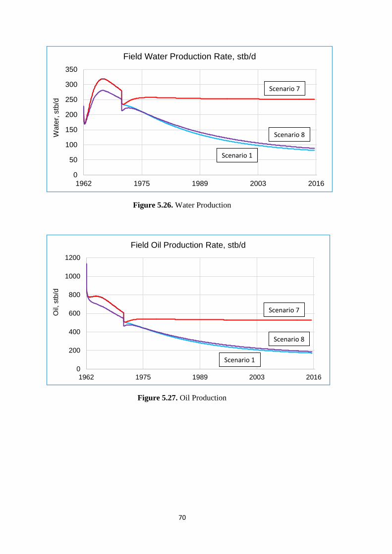
70

Figure 5.26. Water Production

Figure 5.27. Oil Production

0

50

100

150

200

250

300

350

1962 1975 1989 2003 2016

Wa

ter,

stb

/dField Water Production Rate, stb/d

0

200

400

600

800

1000

1200

1962 1975 1989 2003 2016

Oil,

stb

/d

Field Oil Production Rate, stb/d

Scenario 7

Scenario 8

Scenario 1

Scenario 7

Scenario 8

Scenario 1

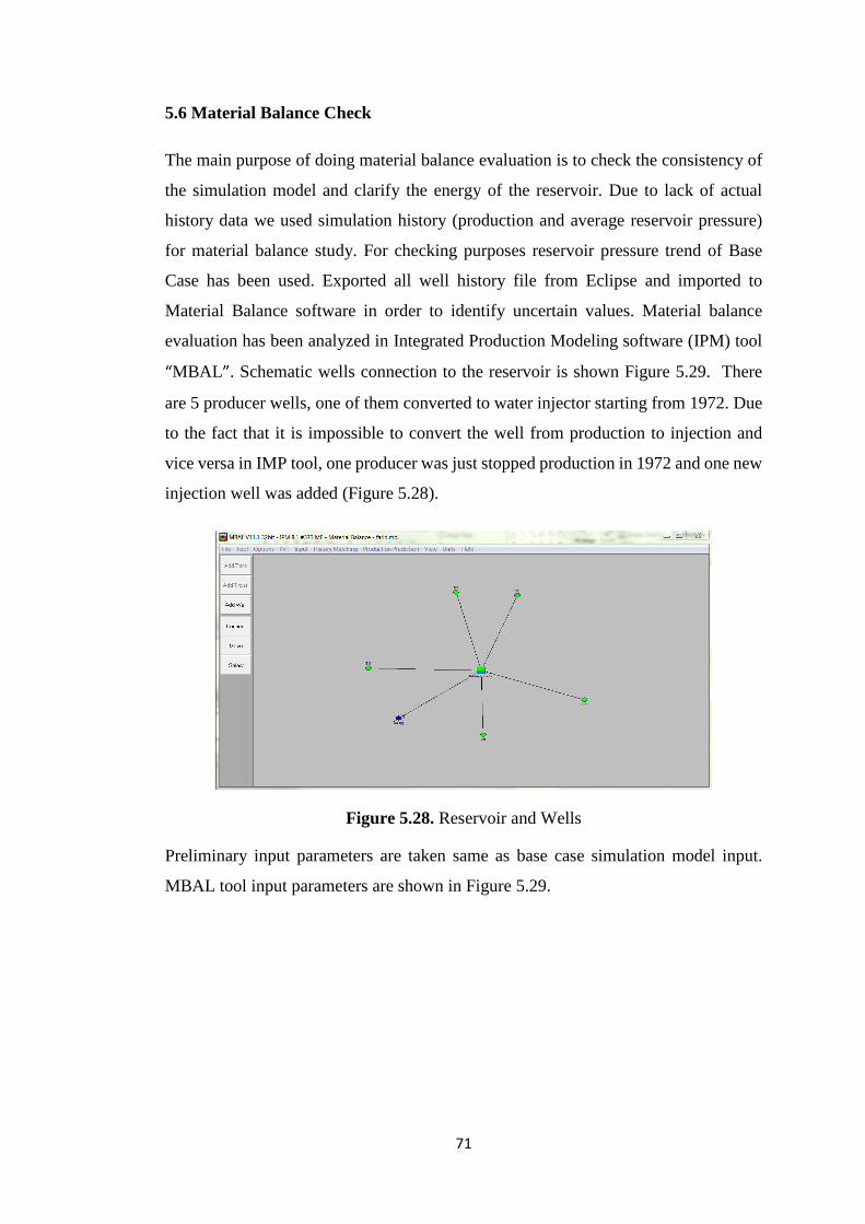
71

5.6 Material Balance Check

The main purpose of doing material balance evaluation is to check the consistency of

the simulation model and clarify the energy of the reservoir. Due to lack of actual

history data we used simulation history (production and average reservoir pressure)

for material balance study. For checking purposes reservoir pressure trend of Base

Case has been used. Exported all well history file from Eclipse and imported to

Material Balance software in order to identify uncertain values. Material balance

evaluation has been analyzed in Integrated Production Modeling software (IPM) tool

“MBAL”. Schematic wells connection to the reservoir is shown Figure 5.29. There

are 5 producer wells, one of them converted to water injector starting from 1972. Due

to the fact that it is impossible to convert the well from production to injection and

vice versa in IMP tool, one producer was just stopped production in 1972 and one new

injection well was added (Figure 5.28).

Figure 5.28. Reservoir and Wells

Preliminary input parameters are taken same as base case simulation model input.

MBAL tool input parameters are shown in Figure 5.29.

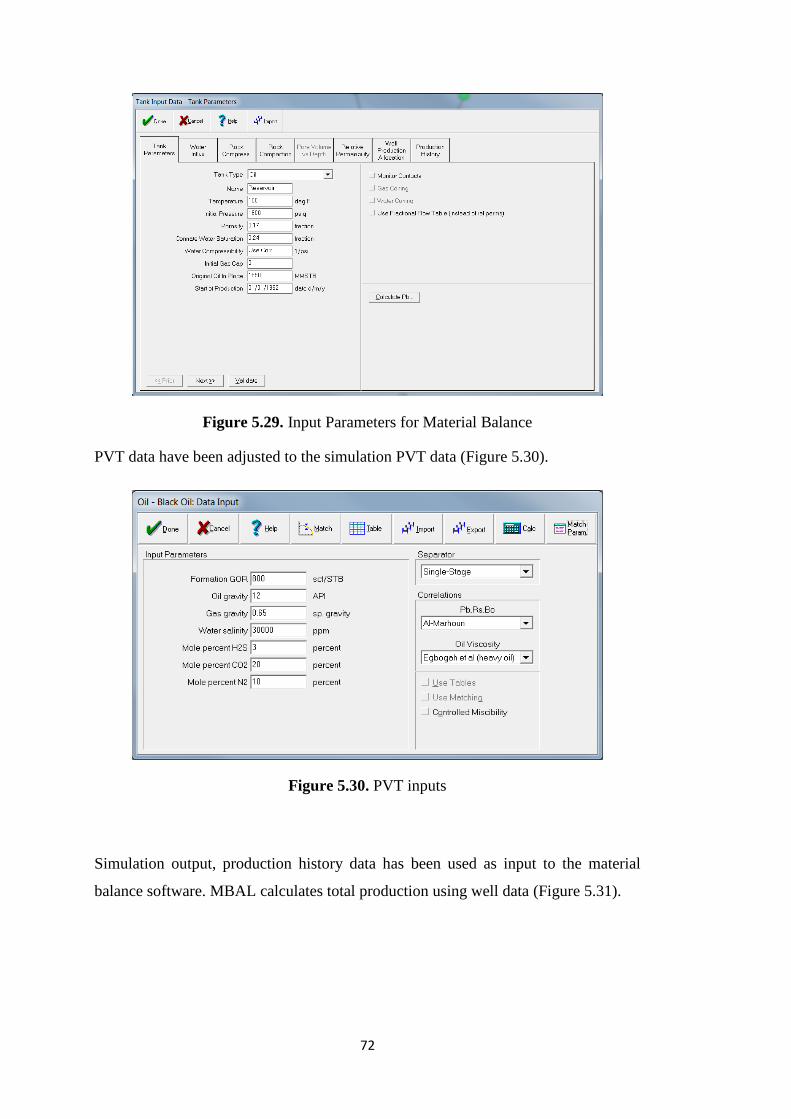
72

Figure 5.29. Input Parameters for Material Balance

PVT data have been adjusted to the simulation PVT data (Figure 5.30).

Figure 5.30. PVT inputs

Simulation output, production history data has been used as input to the material

balance software. MBAL calculates total production using well data (Figure 5.31).

73

Figure 5.31. Production inputs from simulation output

Cumulative injection, production and average reservoir pressure trend are shown in

Figure 5.32.

a)

b)

Figure 5.32. Cumulative Injection, Production and Reservoir Pressure

74

STOIIP preliminary was 1850 MMstb based on simulation model. During history

matching process it has matched to 1833 MMstb (Figure 5.33).

Figure 5.33. Matching Uncertain Parameters

After 8 iterations average reservoir pressure of MBal matched average reservoir

pressure trendline of simulation model. Average reservoir pressure comparison

between material balance and simulation is shown in Figure 5.34. However, those

pressures are not matched ideally, but overall depletion trend is similar. The purpose

of usage of material balance was to check the correctness of simulation model. Thus,

Figure 5.34 provides the outcome of reservoir pressures both from simulation

modeling and material balance. The similarity of reservoir pressure can easily be seen

from Figure 5.34.

75

Figure 5.34. Average Reservoir Pressure comparison between Material Balance and

Simulation

Figure 5.35 shows prevailing drive mechanism versus time. When the reservoir

pressure is less than bubble point pressure, the dominant drive mechanism was fluid

expansion effect from 1962 to 1972 (Figure 5.35). Water injection effect started to

dominate after 1975. Pore volume compressibility effect is negligible for this type of

reservoir. Figure 5.35 clearly demonstrates that for this particular, hypothetical field

implementation of water injection technique is the best case for reservoir energy

support.

Figure 5.35. Drive Mechanism (MBal)

76

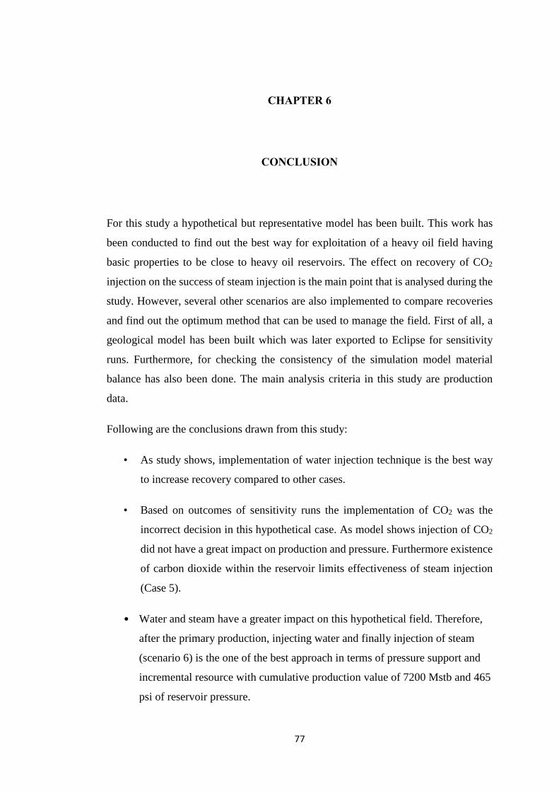
77

CHAPTER 6

CONCLUSION

For this study a hypothetical but representative model has been built. This work has

been conducted to find out the best way for exploitation of a heavy oil field having

basic properties to be close to heavy oil reservoirs. The effect on recovery of CO2

injection on the success of steam injection is the main point that is analysed during the

study. However, several other scenarios are also implemented to compare recoveries

and find out the optimum method that can be used to manage the field. First of all, a

geological model has been built which was later exported to Eclipse for sensitivity

runs. Furthermore, for checking the consistency of the simulation model material

balance has also been done. The main analysis criteria in this study are production

data.

Following are the conclusions drawn from this study:

• As study shows, implementation of water injection technique is the best way

to increase recovery compared to other cases.

• Based on outcomes of sensitivity runs the implementation of CO2 was the

incorrect decision in this hypothetical case. As model shows injection of CO2

did not have a great impact on production and pressure. Furthermore existence

of carbon dioxide within the reservoir limits effectiveness of steam injection

(Case 5).

• Water and steam have a greater impact on this hypothetical field. Therefore,

after the primary production, injecting water and finally injection of steam

(scenario 6) is the one of the best approach in terms of pressure support and

incremental resource with cumulative production value of 7200 Mstb and 465

psi of reservoir pressure.

78

• Pressure outcomes of material balance shows that the simulation model works

properly, as there is a good match among reservoir pressure of simulation

model and material balance.

79

REFERENCES

Ali, Farouq S. M. (1974) “Current Status of Steam Injection as a Heavy Oil Recovery

Method.” Journal of Canadian Petroleum Technology. Volume 13, Number 1.

Ali, Farouq, S. M. and Abou-Kassem, J. H. (1989) “Simulation of thermal recovery

process”, First and second international reservoir simulation, Paul Steiner, Leoben,

Austria.

Ault, J.W., Johnson, W.M., and Kamilos, G.N. (1985) “Conversion of Steamfloods to

Low-Quality Steam and/or Hot-Water Injection Projects”, paper SPE 13604, presented

at the SPE California Regional Meeting, Bakersfield, California, March 27-29.

Baviere, M., 1980. Basic Concepts in Enhanced Oil Recovery Processes. Elsevier

Applied Science, London, New York.

Blair Jr., C. M., Scribner, R. E., and Stout, C. A. (1982) “Chemical Enhancement of

Oil Production by Cyclic Steam Injection”, Journal of Petroleum Technology 34 (12):

2757‐2762.

Blok K, Höhne N, Van der Leun K and Harrison N. “Bridging the greenhouse gas

emissions gap”. 2012

Briggs, P. J. (1989) “A simulator for the recovery of heavy oil from naturally fractured

reservoirs using cyclic steam injection”, paper SPE 17954.

Brissenden, S. J. (2005) “Steaming Uphill: Using J-Wells for CSS at Peace River”,

Canadian International Petroleum Conference, Calgary, Alberta, Jun 7 - 9.

Bryngelsson, M.; Westermark, M. (2009) "CO2 capture pilot test at a pressurized coal

fired CHP plant", Energy Procedia 1: 1403–10.

Burruss, R. (2004) “Geologic Sequestration of Carbon Dioxide in the Next 10 to 50

Years: An Energy Resource Perspective.”

Butler, R. (1991). Thermal Recovery of Oil and Bitumen.

80

Butler, R. M. (2004) “Thermal Recovery of Oil and Bitumen”, 4th edition, GravDrain

Inc, Calgary, Alberta.

Chen, W. H. et. al. (1987) “Thermal simulator for Naturally Fractured Reservoirs”,

paper SPE 14902.

CO2 Surfactants. (n.d.). Retrieved from http://www.novomer.com/co2-surfactants,

September 20, 2014

Conaway, C. F. (1999) “The Petroleum Industry: A Nontechnical Guide”, Pennwell,

Tusla, USA.

Counihan, and Thomas M. A. (1977) “Successful in-situ Combustion Pilot in the

Midway‐Sunset Field, California”, SPE 6525‐MS.

Das, S. (2005) “Improving the Performance of SAGD”, presented at the SPE/PS-

CIM/CHOA International Thermal Operations and Heavy Oil Symposium, Calgary,

Alberta, Canada Nov. 1-3.

De Ghetto, G., Paone, F., and Villa, M. (1995) “Pressure-Volume-Temperature

Correlations for Heavy and Extra Heavy Oils”, SPE 30316.

Dean, R. H., Lo, L. L. (1988) “Simulation of naturally fractured reservoirs”.

Donaldson, E.C., Chilingarian, G.V., Yen, T.F., Sharma, M.K. ʺEnhanced Oil

Recovery, II Processes and Operation.ʺ New York, NY, U.S.A. Elsevier Science

Publishing Company INC. Original publication. ISBN 0‐444‐42933‐6, 1989.

Doscher, T. M. and Ghassemi, F. (1984) ”Limitations on the Oil/Steam Ratio for Truly

Viscous Crudes”.

ECL Technology Report 2 (2001) “CO2 EOR Issues: Phase 1: Literature Review”. UK

DTI SHARP Programme, CO2 dissemination area of DTI SHARP website.

Gozalpour, F. et al. (2005) “CO2 EOR and Storage in Oil Reservoirs”, Oil and Gas

Science and Technology, 60, 3, pp. 537-546.

81

Goodwear, S. G., Hawkyard, I. R., Masters, J. H. K., Woods, C. L., and Jayasekera,

A. J. (2003). Subsurface issues for CO2 flooding of UKCS reservoirs, Trans. IchemE,

81, Part A.

Green, D. W., Willhite, G. P. (1998) “Enhanced Oil Recovery”

Green, D. W. and Willhite, G. P. (2003) “Enhanced Oil Recovery”, Society of

Petroleum Engineers, SPE Textbook Series Vol. 6, Richardson, TX, USA.

Hallam, R.J. and Donnelly, J.K.: “Pressure-Up Blowdown Combustion: A Channelled

Reservoir Recovery process”, presented at the 63rd Annual Technical Conference and

Exhibition of the SPE, Houston, TX, Oct. 2-5, 1988.

Hatzignatiou, D. G., Lu, Y. (1994) “Feasibility Study of CO2 Immiscible Displacement

Process In Heavy Oil Reservoirs”, Annual Technical Meeting, Calgary, Alberta.

Heinrich, J., (2002) “Legal Implications of CO2 Ocean Storage”, Working Paper,

M.I.T., MA, USA, July.

Herbeck, E.F., Heintz, R.C. and Hastings, J.R. (1978) “Fundamentals of Tertiary Oil

Recovery: Part 8 - Thermal Recovery by Hot Fluid Injection”, Petroleum Engineer,

pp. 24-34.

Hong, K.C. (1999) “Recent Advances in Steamflood Technology”, Paper 54078-MS

presented at the International Thermal Operations/Heavy Oil Symposium, Bakersfield,

California, March 17-19.

IPM products, MBal (2010). Retrieved from

http://www.petex.com/products/index.php

Jayasekera, T. et al. (2005) “Optimisation of CO2 Injection into UKCS Oilfields”, 26th

IEA EOR Symposium, Tokyo.

Jespersen, P.J. and Fontaine, T.J.C. (1993) “Tangleflags North Pilot: A Horizontal

Well Steamflood”, J. Can. Petrol. Technol. Vol. 32, No. 5, pp. 52-57.

82

Jessen, K., Kovscek, A. R. and Orr, Jr., F.M. (2005) “Increasing CO2 storage in oil

recovery”. Energy Conversion and Management 46 (2):293-311.

John, F., Cook, M., Graham, M. (1998) “Hydrocarbon Exploration and Production”

Developments in Petroleum Science No. 46, Elsevier, The Netherlands.

Jones, J. and Cawthon, G. J. (1990) “Sequential Steam: An Engineered Cyclic

Steaming Method”.

Kantar K., Karaoguz, D., Issever, K.and Vrana, L. (1985) “Design Concepts of a

Heavy Oil Recovery Process by an Immiscible Process”. Jour. Pet. Tech. February.

Kantar, K., Karaoguz, D., Issever, K., Vrana, L. (1985). "Design Concepts of a Heavy-

Oil Recovery Process by an Immiscible CO2 Application". Journal of Petroleum

Technology 37 (2): 275–283

Kazemi, H., Merrill, L. S. Jr., and Zeman, P. R. (1976) “Numerical Simulation of

Water-Oil Flow in Naturally Fractured Reservoirs”, SPEJ, December.

Khan, J. and Parag, D. (1992) “Twenty-Five Years of Oil Recovery by Steam

Injection.” SPE 24198‐MS.

Kulkarni. M. M. (2003) “Immiscible and Miscible Gas-oil Displacements in Porous

Media”

Leaute, R.P. and Carey, B.S. (2005) “Liquid Addition to Steam for Enhancing

Recovery (LASER) of Bitumen with CSS: Results from the First Pilot Cycle”, paper

2005-161 presented at the Petroleum Society’s 6th Canadian International Petroleum

Conference (56th Annual Technical Meeting), Calgary, Alberta, June 7-9.

Lee, A.L., Gonzalez, M.H., and Eakin, B.E. 1966. The Viscosity of Natural Gases

Lu M, Connell, L. D. (2008) “Non-isothermal flow of carbon dioxide in injection wells

during geological storage”.

McQuarrie, Donald A. and Simon, John D. (1999). Molecular Thermodynamics.

83

Metz, B., O. Davidson, H. C. de Coninck, M. Loos, and L.A. Meyer (eds.) (2005)

“IPCC special report on Carbon Dioxide Capture and Storage”, Prepared by working

group III of the Intergovernmental Panel on Climate Change. Cambridge University

Press, Cambridge, United Kingdom and New York, NY, USA, 442 pp.

Moritis, G. Worldwide EOR Survey. Oil Gas J. 2006.

Oldenburg, C.M., K. Pruess and S. M. Benson, 2001: Process modeling of CO2

injection into natural gas reservoirs for carbon sequestration and enhanced gas

recovery.

Reis, J.C. (1990) “Oil Recovery Mechanisms in Fractured Reservoirs during Steam

Injection,” paper SPE 20204 presented at the SPE/DOE Symposium on Enhanced Oil

Recovery, Tulsa, OK, April 22-25.

Sahuquet, B. C. and Ferrier, J. J. (1982) “Steam-Drive Pilot in a Fractured Carbonate

Reservoir: Lacq Superieur Field,” J. Pet. Tech. April, pp. 873-880.

Satter A., “Heat losses during flow of steam down a wellbore” J. Petroleum

Technology, Vol. 17, 1965

Schulte, W. (2004) “Experience for Use in CO2 for Enhanced Oil Recovery in the

USA”, CO2 conference proceedings, Norway.

Sen, R.,”Biotechnology in petroleum recovery (2008) The microbial EOR”, Progress

in Energy and Combustion Science.

Snøhvit LNG Project PDO support documentation CO2 deposition. Retrieved from

www.statoil.com, 07 June 2001.

Sunnatov, D. (2010) “Experimental Study of Steam Surfactant Flood for Enhancing

Heavy Oil Recovery After Waterflooding”, Master's thesis, Texas A&M University.

Sweet, William (2008) "Winner: Clean Coal - Restoring Coal's Sheen". IEEE

Spectrum45: 57–60.

Thomas, L. K. et.al. (1983) “ Fractured reservoir simulation”

84

Thomas, S. (2008) “Enhanced Oil Recovery – An Overview”, Oil and Gas Science

and Technology, Vol. 63, pp. 9-19.

Tzimas, E. and Peteves, S. (2003) “Controlling Carbon Emissions: The Option of

Carbon Sequestration”, European Commission, EUR Report 20752 EN.

Tzimas, E., Georgakaki, A., Cortes, C. G., and Peteves, S. D. (2005) “Enhanced Oil

Recovery using Carbon Dioxide in the European Energy System”, European

Commission, Report EUR 21895 EN.

Warren, J. E. and Root, P. J.: “The Behavior of Naturally Fractured Reservoirs” SPEJ,

September, 1963., Trans. AIME, 228.

Weinbrandt, R. M. and Ramey, H. J., Jr. (1972) “The Effect of Temperature on

Relative permeability of Consolidated Rocks”, SPE 4142, Annual Meeting, San

Antonio, Oct. 8-11.

West Virginia, carbon sequestration (2008). Retrieved from http://www.wvcarb.org

20 September 2014

Whitson C. and Brule M.: “Phase Behavior”, SPE Monograph Volume 20, Henry

L Doherty Series, Richardson, Texas (2000).

Zhu, C., Zhang, F., and Zhou, J.Z.Q.: “An EOR Application at Liaohe Oil Field in

China – Tests of Pumping Flue Gas into Oil Wells”, presented at the First National

Conference on Carbon Sequestration, Washington D.C., May 15-17, 2001