EFFECTS OF ARRAY SCALING AND ADVANCED … OF ARRAY SCALING AND ADVANCED BEAMFORMING ON THE ANGULAR RESOLUTION OF MICROPHONE ARRAY SYSTEMS ... and the most conventional of the broadband

BeBeC-2016-D1

1

EFFECTS OF ARRAY SCALING AND ADVANCED BEAMFORMING ON THE ANGULAR RESOLUTION OF

MICROPHONE ARRAY SYSTEMS

Matthew Aldeman, Kanthasamy Chelliah, Hirenkumar Patel, and Ganesh Raman Illinois Institute of Technology

10 W. 32nd

Street, Suite 243, Chicago, IL 60616, USA

ABSTRACT

Several advanced beamforming methods have been developed in the past 20 years that

have dramatically improved the angular resolution of microphone array systems.

Meanwhile, the Rayleigh criterion has long been considered the standard criterion for

angular resolution of such systems. In this investigation four microphone arrays were

constructed as scaled models of a fifth microphone array. All of the arrays were

subjected to a thorough regimen of testing with both broadband and narrowband sources.

Using conventional beamforming, the angular resolution of each scaled array was

determined as a function of frequency and compared to the Rayleigh criterion. The

analysis was repeated with the advanced TIDY beamforming algorithm so that the effects

of array scaling and advanced beamforming can be determined as a function of frequency

and compared to conventional beamforming.

1 INTRODUCTION

Microphone array systems have been in use for more than 40 years and have proven

useful in a variety of applications [1]. The most traditional form of beamforming is the Delay-

and-Sum (DAS) beamforming algorithm, wherein time delays are applied to the pressure

signal from each sensor and the resulting signals are summed to form the beamform map [2].

However, the angular resolution of the DAS beamforming algorithm is poor. Frequency-

domain beamforming (FDBF) methods were developed in the 1980’s using the Fast Fourier

Transform. Researchers have since developed improved frequency-domain beamforming

algorithms such as CLEAN, RELAX, and SEM. Many such algorithms are based on the idea

of manipulating the Cross Spectral Matrix and the concept of spatial source coherence

[3,4,5,6,7,8]. More recently, beamforming algorithms have been developed based on methods

of deconvolution [9, 10], methods based on the spatial coherence of point sources and

sidelobes in the frequency domain [11], and spatial coherence methods in the time domain

6th

Berlin Beamforming Conference 2016 Aldeman et al.

2

[12]. These are the DAMAS, DAMAS2, CLEAN-SC, and TIDY algorithms, respectively.

The current investigation will explore the concept of angular resolution utilizing two time-

domain beamforming algorithms: the conventional DAS algorithm and the advanced TIDY

beamforming algorithm.

The most widely-used criterion for the angular resolution of a microphone array system is

the Rayleigh criterion, which indicates that angular resolution is proportional to array

diameter and inversely proportional to the signal’s wavelength. However, the Rayleigh

criterion is a convenient reference point rather than a fixed physical limit. The Rayleigh

resolution criterion defines the angular separation between two sources at the point where the

Airy disk maximum of one source is located at the first minimum of the second source. The

Rayleigh criterion is given by Eq. (1):

𝑊 =

𝑟𝐷

𝜆𝑧 (1)

where r is the separation distance between two adjacent sources, D is the diameter of the

array, λ is the wavelength of the sources and z is the separation distance between the source

and the array. The Rayleigh criterion W is given by the first zero of the first-order Bessel

function of the first kind, divided by a factor of pi to convert into radians. This results in a

value of W = 1.22.

The purpose of this work is to experimentally determine the angular resolution of

microphone arrays as the array size is scaled to larger and smaller dimensions, and to explore

the effect of two beamforming algorithms on the angular resolution of the array. Four

microphone arrays have been constructed as scale models of a fifth baseline microphone

array. All five arrays have been thoroughly tested, and the results were analyzed first with the

conventional DAS algorithm over one-third octave intervals. The results show that the

Rayleigh criterion can be exceeded under certain conditions. The same analysis was then

performed using the TIDY algorithm on the same data. In this way the effect of array scaling

and the effect of the advanced TIDY beamforming method can be determined as a function of

frequency and compared to conventional beamforming.

For the experiments carried out in the following sections, a total of four microphone

arrays were constructed as scale models of a fifth baseline microphone array. The baseline

array has a diameter of 0.73 meters and is hereafter referred to as the “1x” array. An 80%

scale model of this array, called the “0.8x” array was constructed with a diameter of 0.59

meters. Scaled-up versions of the baseline array were constructed with diameters that are

five, ten, and fifteen times larger than the baseline array. The 5x, 10x, and 15x microphone

arrays have diameters of 3.66 meters, 7.32 meters, and 10.98 meters, respectively. Using the

Rayleigh criterion, the expected angular resolution is plotted as a function of frequency for

each of the five microphone arrays in Fig. 1. The resolvable angular resolution between two

acoustic sources (measured in degrees on the horizontal axis) is expected to decrease as either

the diameter of the array is increased or the frequency of the signal is increased.

6th


3

Fig. 1. Expected angular resolution for each of the five microphone arrays.

2 FIVE SCALED MICROPHONE ARRAYS

2.1 Baseline Array

The baseline array on which each of four scaled microphone arrays are based is the 24-

channel OptiNav microphone array produced by OptiNav, Inc. It consists of 24 electret

condenser microphones arranged to approximate a multi-arm spiral pattern with a diameter of

0.73 meters. The microphone pressure signals pass through an amplifier and the data is

acquired with a MOTU 24 I/O 24-channel chassis. Each channel has 24-bit resolution, and

the data is acquired at 44.1 kHz. The MOTU 24 I/O interfaces with a laptop computer

equipped with recording software via a PCIe-424 MAGMA Express Box. The data is saved

on the laptop for later processing using OptiNav’s Beamform Interactive plugin to the ImageJ

image processing software. In addition to the microphones, the microphone array contains a

video camera in the center of the array. The array’s video camera interfaces directly with the

laptop computer via USB connection. The OptiNav compact microphone array is shown in

Fig. 2.

6th


4

Fig. 2. OptiNav compact microphone array and data acquisition chassis

2.2 Four New Scaled Arrays

For comparison against the baseline OptiNav array, four additional microphone arrays

were constructed. The microphone placement within each array is a scaled version of the

OptiNav array geometry. The four newly-constructed arrays consist of one scaled-down array

with a diameter 80% as large as the OptiNav, and three scaled-up arrays that have diameters

of 5, 10, and 15 times greater than the diameter of the OptiNav array. Each array was

constructed with 6mm electret condenser microphones, an amplifier circuit with a gain factor

of 26, and DB25 parallel-port pinout cards for connection to the same MOTU 24 I/O data

acquisition system used by the OptiNav array. The geometry of the array was meticulously

laid out. An image of the completed 0.8x array is shown in Fig. 3.

Fig. 3. Completed 0.8x Array

For the scaled-up arrays, a modular construction approach was necessitated by the size of

the arrays. Each of the 24 microphones was integrated into a combined breadboard

containing the microphone itself and the amplifier circuit. An image of one of the 24 boards

is shown in Fig. 4.

6th


5

Fig. 4. Modular breadboard circuit including microphone (lower left) and amplifier circuit

The array geometry for the 5x, 10x, and 15x arrays was meticulously marked on the roof

of a 21-story building at the Illinois Institute of Technology using exterior-grade painters’

tape. In this way, the location markings for the microphone circuits were semi-permanently

attached, allowing the microphone circuits themselves to be removed when the array was not

in use. When they were to be used, the microphone circuit boards were carefully placed in

alignment with the tape markings. Images of the fully-assembled 5x, 10x, and 15x arrays are

given in Figs. 5, 6, and 7, respectively. In Figs. 6 and 7, the locations of the microphone

circuit boards are circled in red for clarity.

Fig. 5. 3.66m (5x) Microphone array undergoing testing


6th


6


3 ANGULAR RESOLUTION TESTING

Each of the five arrays was subjected to testing at a variety of frequencies, angular

separation values, and both broadband and narrowband sources. The test regimen included

testing each array at 18 frequencies spaced at one-third octave intervals plus a white noise

signal. This sequence was repeated for 19 speaker separation values from 8.9 cm (3.5 in.) to

50.8 cm (20 in.) Thus, the testing sequence involved testing five different microphone arrays

at 18 different frequencies for 19 different speaker separation distances. This made a total of

1,710 test cases. The testing regimen is summarized in Table 1.

Table 1. Angular Resolution Testing Regimen

6th


7

4 RESULTS

The data analysis began by considering the most ubiquitous type of noise source –

broadband – and the most conventional of the broadband beamforming algorithms: Delay-

and-Sum (DAS). The DAS algorithm has been in use for many decades and serves as a

baseline analysis. The DAS algorithm was utilized to construct acoustic source maps for each

array, angular separation value, and one-third octave band using the white noise signal.

Following analysis, the acoustic source map for each set of conditions was judged to a)

consistently resolve the two acoustic sources, b) inconsistently resolve the two acoustic

sources, or c) not resolve the two acoustic sources. The second category, where the algorithm

inconsistently resolves the two sources, was deemed necessary because there were numerous

instances where the algorithm could resolve the sources for certain time steps while it was

unable to resolve the sources in all time steps. This typically occurred near the algorithm’s

resolution limit for a given array geometry and frequency band. Examples of unresolved,

inconsistently resolved, and resolved acoustic sources are given in Fig. 8. The acoustic source

maps are overlaid on the image taken with the array video camera. Although the term

“inconsistently resolved” refers to inconsistency in the time domain, it is apparent in Fig. 8(b)

that the algorithm is very near the resolution limit for this particular set of parameters. Figure

8 shows the results from the 5x array with 25.4 cm (10 in.) of separation between the

speakers, corresponding to an angular separation of 3.1°. The differences between Fig. 8(a),

8(b), and 8(c) are due entirely to the frequency band utilized by the DAS algorithm. Figure

8(a) uses a frequency band of 891-1122 Hz, Fig. 8(b) uses a frequency band of 1413-1778 Hz,

and Fig. 8(c) utilizes frequencies from 2239-2818 Hz.

The discernment between unresolved, inconsistently resolved, and resolved sources is

made more obvious when the acoustic source map is shown by itself against a solid black

background rather than overlaid over an image. Figure 9 shows the same acoustic source

maps without the image of the test apparatus.

(a) (b) (c)

Fig. 8. (a) Unresolved, (b) Inconsistently Resolved, and (c) Resolved noise sources

6th


8

(a) (b) (c)

Fig. 9. (a) Unresolved, (b) Inconsistently Resolved, and (c) Resolved noise sources without images

4.1 DAS Results

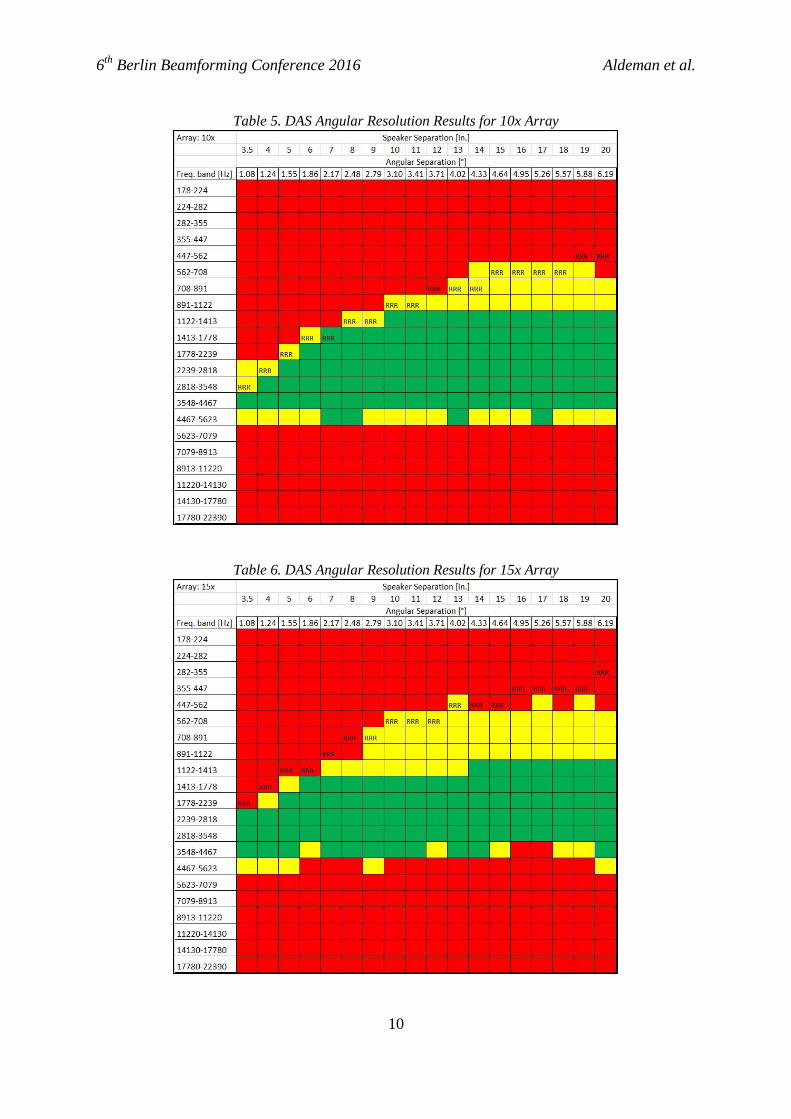
This analysis was carried out using the DAS algorithm for each array, each frequency

band, and each speaker separation distance. The results for the five arrays are given in Tables

2 through 6. In each case, the discretized Rayleigh criterion curve is plotted as “R”s along

with the results. Where the algorithm consistently resolves the two sources, the bin is colored

green. Where the algorithm inconsistently resolves the sources the bin is colored yellow, and

where the algorithm cannot resolve the sources the bin is colored red.

Table 2. DAS Angular Resolution Results for 0.8x Array

6th


9

Table 3. DAS Angular Resolution Results for 1x Array


6th


10



6th


11

The lower operating frequency limit of the arrays, denoted in Tables 2-6 by the uppermost

green and yellow bins, is limited by the ability of the algorithm to resolve two acoustic

sources at low frequencies. It is apparent that the Rayleigh criterion can indeed be exceeded

under certain conditions. It appears that the Rayleigh limit becomes increasingly difficult to

exceed as the array size increases, even though the calculation of the Rayleigh limit already

incorporates the array diameter. This could possibly be due to a source of error discussed in

Section 4.4.

The upper operating frequency limit, denoted in Tables 2-6 by the lowermost green and

yellow bins, is limited by the appearance and subsequent dominance of grating lobes. As the

frequency increases, the inter-element spacing becomes larger relative to the wavelength,

which will eventually lead to grating lobes. At the upper frequency limit, the actual acoustic

sources in the acoustic source map are no longer distinguishable from the grating lobes.

Because each array in this experiment has an identical number of microphones, the inter-

element spacing becomes larger as the array size increases. Thus, the useful upper frequency

limit is reduced as the array size is increased.

4.2 TIDY Results

The analysis described above was repeated using the TIDY beamforming algorithm. The

TIDY algorithm is an advanced time-domain beamforming algorithm useful for improved

beamforming of broadband sources. The results are given below in Tables 7 through 11.

Table 7.TIDY Angular Resolution Results for 0.8x Array

6th


12

Table 8.TIDY Angular Resolution Results for 1x Array

Table 9. TIDY Angular Resolution Results for 5x Array

6th


13



6th


14

Compared to the DAS results in Tables 2-6 the TIDY results show both superior angular

resolution at low frequencies and superior mitigation of grating lobes at high frequencies.

This results in an expanded operating range for the TIDY algorithm as compared to the DAS

algorithm, which appears as an expanded green region in the results tables above. Each one

of the arrays shows a significant increase in performance with the TIDY algorithm as

compared to the DAS algorithm. However, the smaller arrays (0.8x, 1x, 5x) exhibit

particularly large gains in performance, with the gains occurring at both the low and high

frequency edges of the useful operating region.

As the size of the array increased, the angular resolution performance of the array

improved in absolute terms. That is, for a given frequency, a larger array consistently

resolved the sources at a smaller separation angle. However, as the array size increased the

angular resolution performance of the array tended to decrease relative to the Rayleigh

criterion. The 0.8x array greatly exceeded the Rayleigh criterion over its entire useful

operating region, while the performance of the 1x array relative to the Rayleigh criterion was

only slightly lower. The 5x array consistently outperformed the Rayleigh criterion over its

operating range, but its performance relative to the Rayleigh criterion was slightly lower. The

10x array consistently met the Rayleigh criterion over the higher-frequency portion of its

operating range, but as the frequency decreased the 10x array was not able to consistently

meet the Rayleigh criterion. However, the 10x array was able to inconsistently match the

Rayleigh criterion over most of the low-frequency portion of its operating range. Finally, the

15x array came close to meeting the Rayleigh criterion over the high-frequency portion of its

range, but was not able to meet the Rayleigh criterion – even on an inconsistent basis – at the

lowest frequencies. The cause of this relative decrease in performance is not immediately

clear, but several possible explanations are explored in Section 4.4.

When the array size increased, the effective upper frequency limit decreased. This is

expected, and is due to the increasing inter-element spacing as the array size grows larger.

Larger inter-element spacing results in the onset and subsequent dominance of grating lobes at

lower frequencies because the spacing becomes larger relative to the signal wavelength. The

exception to this pattern was between the 0.8x array and the 1x array, where the 1x array had

a higher upper frequency limit than the 0.8x array. This was probably due to the

manufacturing precision of the 1x array as compared to the 0.8x array. The 1x array was built

by OptiNav using precision machining of sheet metal. The 0.8x array was built by the author

out of oak plywood, and while extreme care was taken in order to be as precise as possible,

the placement of the microphones is probably not as precise as the OptiNav array. At very

high frequencies, small microphone placement errors may lead to decreased performance.

4.3 Angular Resolution Comparison by Array Size and Algorithm

A summary of each array’s angular resolution performance can be seen by plotting the

minimum consistently resolvable angular separation for each array at each frequency band.

This type of plot facilitates a simple comparison of angular resolution between arrays. Fig. 10

shows the minimum consistently resolvable angular separation for each array using the DAS

algorithm, and Fig. 11 shows the minimum consistently resolvable angular separation for each

array using the TIDY algorithm.

6th


15

Fig. 10. Minimum Angular Resolution Data for 0.8x, 1x, 5x, 10x, and 15x arrays using DAS

algorithm

Fig. 11. Minimum Angular Resolution Data for 0.8x, 1x, 5x, 10x, and 15x arrays using DAS

algorithm

6th


16

Several observations can be made from inspection of Figs. 10 and 11. First, the minimum

resolvable separation almost always decreases when the array size increased, as expected.

Second, the arrays clearly have different operating bands. Thus, a different array may be

selected for an application depending on the frequency of the expected signal. Finally,

comparison of the DAS and TIDY plots shows that the TIDY algorithm provides superior

angular resolution. For a given array, the angular resolution curve in the TIDY plot is

generally shifted down (to smaller angular separation values) and/or shifted left (to lower

frequencies) as compared to the DAS plot.

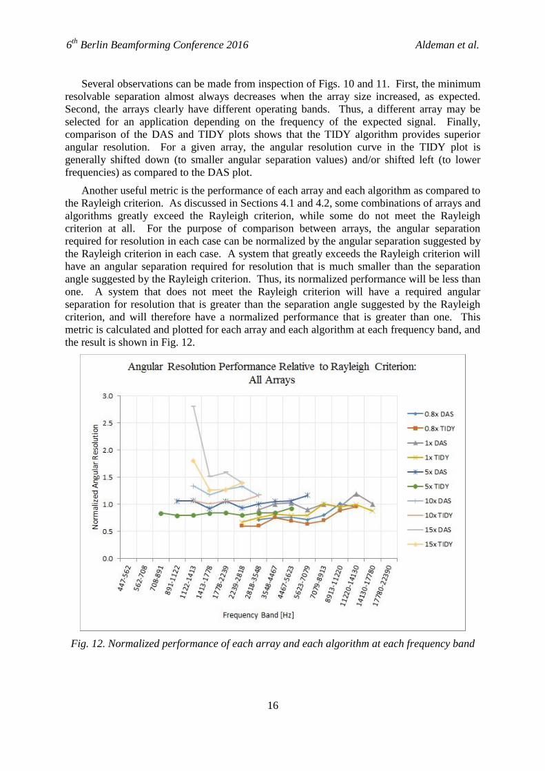
Another useful metric is the performance of each array and each algorithm as compared to

the Rayleigh criterion. As discussed in Sections 4.1 and 4.2, some combinations of arrays and

algorithms greatly exceed the Rayleigh criterion, while some do not meet the Rayleigh

criterion at all. For the purpose of comparison between arrays, the angular separation

required for resolution in each case can be normalized by the angular separation suggested by

the Rayleigh criterion in each case. A system that greatly exceeds the Rayleigh criterion will

have an angular separation required for resolution that is much smaller than the separation

angle suggested by the Rayleigh criterion. Thus, its normalized performance will be less than

one. A system that does not meet the Rayleigh criterion will have a required angular

separation for resolution that is greater than the separation angle suggested by the Rayleigh

criterion, and will therefore have a normalized performance that is greater than one. This

metric is calculated and plotted for each array and each algorithm at each frequency band, and

the result is shown in Fig. 12.

Fig. 12. Normalized performance of each array and each algorithm at each frequency band

6th


17

The lower curves in Fig. 12 represent the best angular resolution performance relative to

the Rayleigh criterion. In general, Fig. 12 shows that the smaller arrays tend to outperform

the large arrays relative to the Rayleigh criterion, and that the TIDY algorithm tends to

outperform DAS. Thus, the lower curves in Fig. 12 (representing the best performance

relative to the Rayleigh criterion) are dominated by the smaller arrays and the TIDY

algorithm, while the upper curves generally represent the larger arrays and the DAS

algorithm.

4.4 Addressing Potential Sources of Error

The DAS and TIDY results presented in the previous sections exhibit profiles that

approximate the shape of the Rayleigh curve. However, the relative performance of the

arrays compared to each other is not thoroughly explained by the Rayleigh criterion alone.

For example, the smaller 0.8x and 1x arrays easily outperform the Rayleigh criterion by

significant margins. Meanwhile, the larger 10x and 15x arrays are only barely capable of

meeting the Rayleigh criterion, and in some cases cannot meet the Rayleigh criterion. There

are several possible reasons for this:

i. Signal-to-Noise Ratio (SNR): It is possible that the larger arrays – especially at the

outside edges – are suffering from poor SNR. This may reduce the effective

diameter of the array, thereby reducing the low-frequency performance.

ii. Z-axis correction: The initial testing and analysis described above was performed

with the assumption that the rooftop under the arrays is a perfectly flat horizontal

plane. Accurately measuring and re-analyzing the data with corrected z-axis

measurements may improve the results.

iii. Signal reflection effects: The arrays are assumed to be operating in a free field

environment, but of course this is not entirely accurate. The roof has a concrete

safety barrier approximately 1 meter tall extending around the perimeter of the

roof. As the array size increases, the microphones must be positioned closer to the

barrier. Reflection of the test signal off the concrete perimeter barrier may

adversely affect the performance of the larger arrays.

Signal-to-Noise Ratio (SNR) Effects

Potential SNR issues could be adversely affecting the output of the larger arrays. The

SNR may be acceptable for the smaller arrays because they are closer to the acoustic test

sources. But as the radius of the array increases and the array elements become farther away

from the test sources, the SNR could decrease. This could reduce the effective diameter of

the larger arrays, which would impair the ability of the array to resolve sources at low

frequencies. Fortunately, there is a relatively simple test to check if poor SNR is affecting the

beamforming output. To check for SNR impacts, the integration time for the beamforming

map can be varied. If SNR is adversely affecting the output, then the results will improve

with longer integration times. If SNR is not significantly affecting the output, then the

beamforming results will vary little as the integration time is changed. This check was

performed for both DAS and TIDY algorithms across several different angular separation

distances and for different initial beamforming results (i.e. green, yellow, and red cells in

Tables 2-11). For brevity, only one such example case will be given here. Because it may

6th


18

offer the best chance to show improvement, a marginal or “yellow” (inconsistently resolved)

case will be shown below. The inconsistently resolved case for the 15x array at 20.3cm (8

in.) speaker separation with the DAS algorithm at 1122-1413 Hz is given in Fig. 13.

(a) (b)

(c) (d)

(e) (f)

Fig. 13. Beamforming map for 15x array at 20.3cm (8in.) speaker separation with DAS

algorithm at 1122-1413 Hz using integration times of (a) 0.1s, (b) 0.2s, (c) 0.4s, (d) 0.8s,

(e) 2.0s, and (f) 4.0s.

6th


19

As can be seen in Fig. 13, the beamforming map does not significantly change as the

integration time is varied from 0.1s to 4.0s. This effect is consistent across both algorithms,

all source separation distances, and regardless of initial beamforming result. This indicates

that the SNR is not significantly affecting the beamforming output.

Z-axis Correction

When the 5x, 10x and 15x microphone arrays were laid out on the rooftop, it was assumed

that the roof was a flat horizontal plane. Even if this is not true, the error was assumed to be

small. However, errors in z position could be affecting the results. To address this potential

issue, z-axis measurements were taken and the results were re-analyzed with the corrected

microphone position geometry.

To measure the z-axis position of the microphone array elements, a rotary laser level was

placed at the center of each array and leveled. A measuring stick was then placed at every

microphone position, and the height of the laser level plane above the microphone position

was recorded. By subtracting the average z measurement from each individual measurement,

the z-axis coordinate of each microphone was obtained. The average magnitude (absolute

value) of the z correction for individual elements in the 5x array was 1.0 cm (0.41 in.), while

for the 10x and 15x arrays the average magnitude of the z corrections were 2.8 cm (1.12 in.)

and 3.3 cm (1.31 in.), respectively. The array geometry was updated with the corrected z-axis

coordinates and the beamforming analysis was re-performed for each case. For brevity the

full results tables are not shown here, but the effects are discussed below.

The z-axis correction could potentially impact the beamforming results in two distinct

ways. It could impact the arrays’ ability to resolve low frequency sources, i.e. it may affect

the angular resolution performance relative to the Rayleigh criterion. Alternatively or

additionally, the correction may impact the upper frequency limit of the array, i.e. the

maximum frequency at which the array can effectively operate before the onset and

dominance of grating lobes. Each of these possibilities will be tested separately.

The effect of z-axis correction on the performance of the array relative to the Rayleigh

criterion will be discussed first. To show this potential effect, the minimum frequency at

which the beamforming map was able to consistently resolve sources at each angular

separation distance was recorded. This is analogous to the upper-most green cell in each

column of Tables 2-11. This may be considered the “angular resolution frontier.” It is the

curve representing the lowest frequency at which the algorithm can consistently resolve two

acoustic sources at a given angular separation. The angular resolution frontier curves for

uncorrected and z-corrected analysis of each array are presented in Fig. 14 (DAS) and Fig. 15

(TIDY). The data for the 0.8x and 1x arrays is not shown because the microphones on the

smaller arrays were installed on a flat plate rather than the rooftop. Therefore there is no z

correction for the 0.8x and 1x arrays.

6th


20

Fig. 14. Angular resolution frontier curve for uncorrected and z-corrected analysis of 5x, 10x,

and 15x arrays with the DAS algorithm

Fig. 15. Angular resolution frontier curve for uncorrected and z-corrected analysis of 5x, 10x,

and 15x arrays with the TIDY algorithm.

6th


21

A number of conclusions can be drawn from inspection of Figs. 14 and 15. First, it is

apparent that for a given angular separation, the TIDY algorithm is able to achieve resolution

at a lower frequency band than the DAS algorithm. This is consistent with earlier discussion

in Sections 4.2 and 4.3. Second, it is also apparent that a larger array is usually able to

achieve resolution for a given angular separation at a lower frequency band than a smaller

array. Finally, it can be seen that the uncorrected and z-corrected curves for a particular array

generally lie on top of each other. That is, the uncorrected and z-corrected angular resolution

frontier curves are nearly identical. This means that the z-axis correction did not significantly

impact the angular resolution performance of the arrays relative to the Rayleigh criterion.

This is logical, as the signal wavelengths in this region are on the order of 10-35 cm while the

average z errors are on the order of 1-3 cm. Therefore, the data and the plots in Section 4.3

remain essentially unchanged.

The effect of z-axis correction on the upper frequency limit of the array will be analyzed

next. The upper frequency limit is the maximum frequency that the beamforming system can

achieve before grating lobes dominate the beamform map. In contrast to the low-frequency

resolution, the upper frequency limit of the array does not depend on angular separation of the

sources. This can be seen in Tables 2-11, where the bottom edge of the green region is a

roughly horizontal line segment. Because it does not depend on angular separation of the

sources, an average can be taken across all angular separation values for each array and

algorithm. By averaging the maximum frequency achieved by each array and each algorithm

with both uncorrected and z-corrected geometries, the effect of z correction on the upper

frequency limit can be determined. The average upper frequency limits are shown in Fig. 16

(DAS) and Fig. 17 (TIDY).

Fig. 16. Average Maximum Frequency for uncorrected and z-corrected geometry with 5x,

10x, and 15x arrays using DAS algorithm

6th


22

Fig. 17. Average Maximum Frequency for uncorrected and z-corrected geometry with 5x,

10x, and 15x arrays using TIDY algorithm

By inspection of Figs. 16 and 17 it is apparent that z-coordinate correction has a

significant impact on the upper frequency limit. In every case, z correction improved the

upper frequency limit of the array system. The effect was most pronounced with the 5x array.

This is likely because the smaller inter-element spacing of the 5x array meant that it had

greater potential to operate at higher frequencies, but it could not do so without precise

microphone placement geometry. Even the 15x array showed significant improvement,

although it showed less improvement than the 5x and 10x arrays. This is likely because the

larger inter-element spacing of the 15x array means that it is not capable of operating at very

high frequencies even with very precise microphone placement.

Signal Reflection Effects at Boundaries

Another potential source of error is the possibility of signal reflection effects at

boundaries near the edge of the larger arrays. The arrays are assumed to be operating in a free

field environment, but of course this is not entirely accurate. In addition to various ventilation

equipment located on the rooftop, the roof has a concrete safety barrier approximately 1 meter

tall extending around the perimeter of the roof. As the array size increases, the microphones

must be located closer to the concrete barrier. In the largest (15x) array, the closest

microphone is located approximately one meter from the wall. Reflection of the test signal

off the concrete perimeter barrier may adversely affect the performance of the larger arrays.

To test this hypothesis, an experiment will be conducted in a controlled laboratory

environment. Several array geometries will be laid out on a horizontal surface in an open

laboratory environment approximating a free field. A complete battery of angular resolution

testing will be performed using the same test apparatus that was used to test the arrays on the

roof. Next, a barrier will be constructed around the perimeter of the array. The angular

resolution testing will be repeated. The results from these test conditions will be compared,

6th


23

and the comparison will provide empirical insight into the effect of perimeter boundary

reflection.

5 SUMMARY

A series of experiments was conducted to determine the operating characteristics of five

scaled microphone arrays. It is apparent from the tables of results that each array has a

different operating range in terms of frequency and angular resolution. This reinforces the

fact that the important performance characteristics of an array must be specified at an early

stage of development so that the important parameters of the array can be designed

accordingly. For increased angular resolution, the array should have a large diameter and/or it

should operate at high frequencies. To increase the upper frequency limit of the useful

operating range, the inter-element spacing should be kept small compared to the wavelength

of interest.

The results of these experiments show the angular resolution of each array using the DAS

beamforming algorithm as well as the TIDY algorithm compared against the Rayleigh

criterion curve. TIDY is shown to outperform the DAS algorithm in nearly every case. In

some cases, especially with smaller arrays using the TIDY algorithm, the Rayleigh criterion

can be significantly exceeded. In other cases, especially with larger arrays and the DAS

algorithm, it is very difficult to achieve resolution meeting the Rayleigh criterion. The next

step will be to perform the same angular resolution analysis using several other advanced

beamforming algorithms such as DAMAS, DAMAS2 and CLEAN-SC. In addition, an

experiment will be performed in a controlled laboratory environment to explore the effect of

perimeter boundary reflection on the angular resolution of microphone arrays.

REFERENCES

[1] Michel, U. “History of Acoustic Beamforming.” Berlin Beamforming Conference,

Berlin. 2006.

[2] Johnson, D.H. & Dudgeon, D.E. Array Signal Processing: Concepts and Techniques.

Prentice Hall. 1993.

[3] R.P. Dougherty, R.W. Stoker. “Sidelobe suppression for phased array aeroacoustic

measurements.” American Institute of Aeronautics and Astronautics Paper 98-2242.

1998.

[4] R.P. Dougherty. “Beamforming in Acoustic Testing”, in T.J. Mueller (ed.) Aeroacoustic

Measurements. Springer. New York. 2002.

[5] S. Oerlemans, P. Sijtsma. “Determination of Absolute Levels from Phased Array

Measurements using Spatial Source Coherence.” American Institute of Aeronautics and

Astronautics Paper 2002-2464. 2002.

[6] T.F. Brooks, W.M. Humphreys Jr. “Flap Edge Aeroacoustic Measurements and

Predictions.” J. Sound Vib. 261, 31-74. 2003.

6th


24

[7] Y. Wang, J. Li, P. Stoica, M. Sheplak, T. Nishida. “Wideband RELAX and wideband

CLEAN for aeroacoustic imaging.” American Institute of Aeronautics and Astronautics

Paper 2003-3197. 2003.

[8] D. Blacodon, G. Elias. “Level Estimation of Extended Acoustic Sources using an Array

of Microphones.” American Institute of Aeronautics and Astronautics Paper 2003-3199.

2003.

[9] T.F. Brooks and W.M. Humphreys, Jr. “A Deconvolution Approach for the Mapping of

Acoustic Sources (DAMAS) determined from phased microphone array.” J. Sound Vib.

294 (4-5), 856-879. 2006.

[10] R.P. Dougherty. “Extensions of DAMAS and Benefits and Limitations of

Deconvolution in Beamforming.” American Institute of Aeronautics and Astronautics

Paper 2005-2961. 2005.

[11] P. Sijtsma. “CLEAN based on spatial source coherence.” Int. J. Aeroacoustics, 6, 357–

374, 2007.

[12] R.P. Dougherty and G. Podboy. “Improved Phased Array Imaging of a Model Jet.”

American Institute of Aeronautics and Astronautics Paper 2009-3186. 2009.

Documents

EFFECTS OF ARRAY SCALING AND ADVANCED … OF ARRAY SCALING AND ADVANCED BEAMFORMING ON THE ANGULAR RESOLUTION OF MICROPHONE ARRAY SYSTEMS ... and the most conventional of the broadband