EFFECTS OF A SINGLE MAGNETIC

IMPURITY ON SUPERCONDUCTIVITY

A Thesis Submitted to the

College of Graduate Studies and Research

in Partial Fulfillment of the Requirements

for the degree of Master of Science

in the Department of Physics and Engineering Physics

University of Saskatchewan

Saskatoon

By

Sushan Pan

c©Sushan Pan, November/2008. All rights reserved.

Permission to Use

In presenting this thesis in partial fulfilment of the requirements for a Postgrad-

uate degree from the University of Saskatchewan, I agree that the Libraries of this

University may make it freely available for inspection. I further agree that permission

for copying of this thesis in any manner, in whole or in part, for scholarly purposes

may be granted by the professor or professors who supervised my thesis work or, in

their absence, by the Head of the Department or the Dean of the College in which

my thesis work was done. It is understood that any copying or publication or use of

this thesis or parts thereof for financial gain shall not be allowed without my written

permission. It is also understood that due recognition shall be given to me and to the

University of Saskatchewan in any scholarly use which may be made of any material

in my thesis.

Requests for permission to copy or to make other use of material in this thesis in

whole or part should be addressed to:

Head of Department of Physics and Engineering Physics

116 Science Place

University of Saskatchewan

Saskatoon, Saskatchewan

Canada

S7N 5E2

i

Abstract

Electronic structure of a conventional superconductor in the vicinity of a single, iso-

lated magnetic impurity has been probed experimentally with scanning tunneling

spectroscopy by Yazdani et al.. Motivated by their experiment, we study the ef-

fects of a single magnetic impurity on superconductivity by means of the mean-field

Bogoliubov-de Gennes theory. The Bogoliubov-de Gennes equations are solved di-

rectly and numerically, utilizing parallel computation on a CFI-founded 128-CPU

Beowulf-class PC cluster here at the University of Saskatchewan. As a preliminary

study, we also examine the electronic structure around a magnetic vortex. The local

magnetic field around a vortex breaks up Cooper pairs and suppresses superconduc-

tivity locally. Quasiparticle excitations are created and bound in the vortex core area

due to repeated Andreev scattering. A magnetic impurity tends to align the spins of

the neighboring electrons and break up Cooper pairs, and has similar effects of lo-

cally suppressing superconductivity. A striking difference, however, from the vortex

problem is that around a magnetic impurity there is particle-hole asymmetry in the

tunneling conductance. This is due to different probability amplitudes in the spin-up

branch and the spin-down branch of quasiparticle excitations. Furthermore, for the

spin potential strength larger than a certain critical value, the nature of quasiparticle

excitations is changed dramatically. Within a model of classical spin, we propose an

explanation of the measured tunneling conductance of the experiment. This work

is significant in that it gives us insight into superconductivity and magnetism–two

complementary manifestation of strong electron correlations.

ii

Acknowledgements

I would like to thank my supervisor, Dr. Kaori Tanaka, for her guidance and

support throughout this project. I would also like to thank my committee members,

Drs. Gap Soo Chang, Rainer Dick and Glenn Hussey, and the external examiner Dr.

Chris Soteros for helpful comments and discussions. Financial support by the Natural

Sciences and Engineering Research Council of Canada is gratefully acknowledged. I

am also grateful to the support staff of the Department of Physics and Engineering

Physics.

iii

This thesis is dedicated to my parents, Pan and Hong

iv

Contents

Permission to Use i

Abstract ii

Acknowledgements iii

Contents v

List of Figures vii

List of Abbreviations ix

1 Introduction 11.1 Motivation . . . . . . . . . . . . . . . . . . . . . . . . . . . . . . . . . 1

1.1.1 Magnetic Properties of Superconductors . . . . . . . . . . . . 11.1.2 Effects of a Magnetic Impurity . . . . . . . . . . . . . . . . . . 6

1.2 BCS Theory . . . . . . . . . . . . . . . . . . . . . . . . . . . . . . . . 81.3 BdG Theory . . . . . . . . . . . . . . . . . . . . . . . . . . . . . . . . 15

2 Electronic Structure around a Vortex 192.1 Motivation . . . . . . . . . . . . . . . . . . . . . . . . . . . . . . . . . 192.2 Material . . . . . . . . . . . . . . . . . . . . . . . . . . . . . . . . . . 192.3 Homogeneous System . . . . . . . . . . . . . . . . . . . . . . . . . . . 20

2.3.1 Formulation . . . . . . . . . . . . . . . . . . . . . . . . . . . . 202.3.2 Results and Discussion . . . . . . . . . . . . . . . . . . . . . . 22

2.4 Isolated Vortex . . . . . . . . . . . . . . . . . . . . . . . . . . . . . . 242.4.1 Formulation . . . . . . . . . . . . . . . . . . . . . . . . . . . . 242.4.2 Results and Discussion . . . . . . . . . . . . . . . . . . . . . . 28

3 Electronic Structure around a Magnetic Impurity 353.1 Homogeneous System . . . . . . . . . . . . . . . . . . . . . . . . . . . 36

3.1.1 Formulation . . . . . . . . . . . . . . . . . . . . . . . . . . . . 363.1.2 Results and Discussion . . . . . . . . . . . . . . . . . . . . . . 38

3.2 Isolated Magnetic Impurity . . . . . . . . . . . . . . . . . . . . . . . 383.2.1 Formulation . . . . . . . . . . . . . . . . . . . . . . . . . . . . 383.2.2 Results and Discussion . . . . . . . . . . . . . . . . . . . . . . 42

4 Conclusion 584.1 Conclusion . . . . . . . . . . . . . . . . . . . . . . . . . . . . . . . . . 58

References 63

v

A Parallel Computation 64A.1 Hardware . . . . . . . . . . . . . . . . . . . . . . . . . . . . . . . . . 64A.2 Software . . . . . . . . . . . . . . . . . . . . . . . . . . . . . . . . . . 64A.3 Computation . . . . . . . . . . . . . . . . . . . . . . . . . . . . . . . 67

A.3.1 Homogeneous System in Two Dimensions . . . . . . . . . . . . 67A.3.2 Isolated Vortex Problem . . . . . . . . . . . . . . . . . . . . . 67A.3.3 Homogeneous System in Three Dimensions . . . . . . . . . . . 67A.3.4 Isolated Magnetic Impurity Problem . . . . . . . . . . . . . . 67

B Curve Fitting 69B.1 Trigonometric Polynomial Approximation . . . . . . . . . . . . . . . 69B.2 Fitting the Pairing Potential . . . . . . . . . . . . . . . . . . . . . . . 69

vi

List of Figures

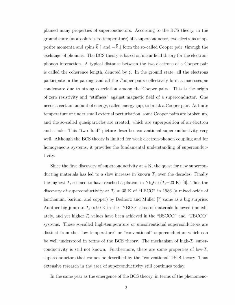
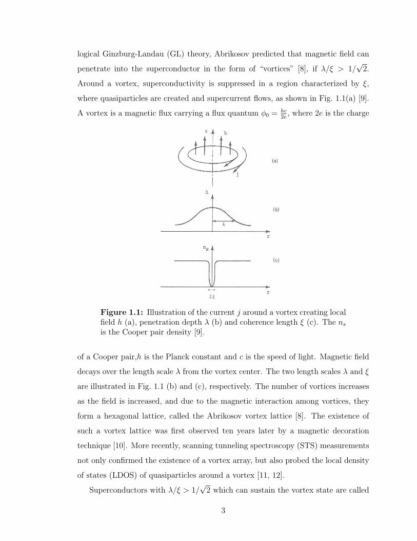
1.1 Illustration of the current j around a vortex creating local field h (a),penetration depth λ (b) and coherence length ξ (c). The ns is theCooper pair density [9]. . . . . . . . . . . . . . . . . . . . . . . . . . . 3

1.2 The field-temperature phase diagram of a type-II superconductor withthree critical fields. Here T0 ≡ Tc is the zero-field transition tempera-ture [9]. . . . . . . . . . . . . . . . . . . . . . . . . . . . . . . . . . . 4

1.3 Tunneling conductance of the experiment of Ref.[20]; of a pure sample(A) and over a magnetic impurity (B). . . . . . . . . . . . . . . . . . 7

1.4 Difference spectra measured near an isolated (A) Mn, (B) Gd, and(C) Ag atom [20]. . . . . . . . . . . . . . . . . . . . . . . . . . . . . . 8

1.5 Quasiparticle excitation energy as a function of momentum k. ThekF and EF are the Fermi momentum and Fermi energy, respectively[24]. . . . . . . . . . . . . . . . . . . . . . . . . . . . . . . . . . . . . 14

1.6 In the superconducting state, energy gap is created around E = EF .The ε is the single-particle kinetic energy measured from EF . TheNn(E) and Ns(E) are the DOS in the normal state and supercon-ducting state, respectively [25]. . . . . . . . . . . . . . . . . . . . . . 14

1.7 Temperature dependance of measured energy gap for various conven-tional superconductors. The curve is the BCS prediction [9]. . . . . . 15

2.1 Normalized tunneling conductance of a pure NbSe2 at temperature T= 1 K, 2 K, 5 K and 7 K. . . . . . . . . . . . . . . . . . . . . . . . . 23

2.2 LDOS of a pure NbSe2 at temperature T = 1 K, 2 K, 5 K and 7 K. . 24

2.3 Uniform order parameter ∆ as a function of temperature. . . . . . . . 25

2.4 Converged order parameter around a vortex for various temperatures. 29

2.5 Energy levels of quasiparticle states as a function of angular momen-tum l. . . . . . . . . . . . . . . . . . . . . . . . . . . . . . . . . . . . 31

2.6 Electron and hole amplitudes of the quasiparticle bound state arounda vortex for l = 1/2 and T = 1 K. . . . . . . . . . . . . . . . . . . . . 32

2.7 Electron and hole amplitudes of the lowest-energy scattering statearound a vortex. . . . . . . . . . . . . . . . . . . . . . . . . . . . . . 33

2.8 Tunneling conductance around a vortex for T = 1 K. . . . . . . . . . 33

2.9 Tunneling conductance at various distances from the vortex center,obtained from Fig. 2.8. . . . . . . . . . . . . . . . . . . . . . . . . . . 34

2.10 Tunneling conductance measured around a vortex in NbSe2 at T = 0.3K by Hess et al. [26]. . . . . . . . . . . . . . . . . . . . . . . . . . . . 34

3.1 Tunneling conductance of a pure Nb at temperature T=1 K. . . . . . 39

3.2 Order parameter around a magnetic impurity for different strengthsof the spin potential. . . . . . . . . . . . . . . . . . . . . . . . . . . . 44

vii

3.3 Order parameter at r = 0 as a function of the spin potential strengthVs. The critical values Vc and V ′

c are indicated. . . . . . . . . . . . . . 453.4 Energies of the bound states with the angular momentum l = 0, 1 as

a function of the spin potential strength. . . . . . . . . . . . . . . . . 463.5 Electron and hole amplitudes of the l = 0 bound state. . . . . . . . . 473.6 Electron and hole amplitudes of a l = 0 scattering state. . . . . . . . 483.7 Phase shift between the electron and hole amplitudes of the spin-up

bound state as a function of the spin potential strength Vs. . . . . . . 493.8 Tunneling conductance of as a function of bias voltage on top of the

magnetic impurity, for three different values of potential strength Vs. 503.9 Difference spectra measured near isolated (A) Mn, (B) Gd, and (C)

Ag atom [20]. . . . . . . . . . . . . . . . . . . . . . . . . . . . . . . . 513.10 Tunneling conductance on top of the magnetic impurity as a function

of bias voltage and spin potential strength Vs. . . . . . . . . . . . . . 523.11 Same as Fig. 3.10 but for larger Vs. . . . . . . . . . . . . . . . . . . . 533.12 Tunneling conductance as a function of energy eV at different radial

distances r. . . . . . . . . . . . . . . . . . . . . . . . . . . . . . . . . 543.13 Tunneling conductance as a function of bias voltage and radial dis-

tance r for Vs = 916 meV. . . . . . . . . . . . . . . . . . . . . . . . . 553.14 Same as Fig. 3.13 but for Vs = 600 meV. . . . . . . . . . . . . . . . . 563.15 Same as Fig. 3.13 but for Vs = 1200 meV. . . . . . . . . . . . . . . . 57

A.1 A shared memory architecture . . . . . . . . . . . . . . . . . . . . . . 65A.2 A distributed memory architecture . . . . . . . . . . . . . . . . . . . 65A.3 Message Passing Interface model . . . . . . . . . . . . . . . . . . . . . 66A.4 Flow Chart of the Computation . . . . . . . . . . . . . . . . . . . . . 66

viii

List of Abbreviations

Tc critical temperatureHc critical magnetic fieldSTM scanning tunneling microscopeSTS scanning tunneling spectroscopyLDOS local density of statesDOS density of statesBdG the Bogoliubov-de Gennes theoryBCS the Bardeen-Cooper-Schrieffer theoryCdM Caroli, de Gennes, and MatriconGS Gygi and SchluterGL the Ginzburg-Landau theoryMPI message passing interface

ix

Chapter 1

Introduction

1.1 Motivation

1.1.1 Magnetic Properties of Superconductors

Superconductivity is a phenomenon first discovered by Kamerlingh Onnes in 1911

[1]. In his experiment, he found that electrical resistivity of mercury dropped sharply

to zero when temperature T was decreased below a critical value Tc (4 K for mer-

cury). This property of a superconductor holds if the magnitude of the electrical

current is smaller than a critical value Jc. In addition to this perfect conductivity, a

key feature that distinguishes a superconductor from a perfect conductor is perfect

diamagnetism, the so-called Meissner effect discovered by Meissner and Ochsenfeld

in 1933 [2]. Both a perfect conductor and a superconductor exclude magnetic field.

However, when magnetic field is applied before cooling down, perfect conductivity

and superconductivity show different properties. While a perfect conductor keeps

trapping the field, a superconductor expels the magnetic field for T < Tc. Diamag-

netism in the interior of the superconductor is maintained by supercurrent on the

surface. The thickness of the region where the supercurrent exists and magnetic field

is nonzero, is called the penetration depth, denoted by λ. This distinct property of

a superconductor is lost for the field strength larger than a critical value Hc. At

Hc, the magnitude of supercurrent exceeds Jc and thus the material can no longer

maintain superconductivity.

In 1957, Bardeen, Cooper and Schrieffer proposed a microscopic theory, the so-

called Bardeen-Cooper-Schrieffer (BCS) theory [3, 4, 5], which has successfully ex-

1

plained many properties of superconductors. According to the BCS theory, in the

ground state (at absolute zero temperature) of a superconductor, two electrons of op-

posite momenta and spins ~k ↑ and −~k ↓ form the so-called Cooper pair, through the

exchange of phonons. The BCS theory is based on mean-field theory for the electron-

phonon interaction. A typical distance between the two electrons of a Cooper pair

is called the coherence length, denoted by ξ. In the ground state, all the electrons

participate in the pairing, and all the Cooper pairs collectively form a macroscopic

condensate due to strong correlation among the Cooper pairs. This is the origin

of zero resistivity and “stiffness” against magnetic field of a superconductor. One

needs a certain amount of energy, called energy gap, to break a Cooper pair. At finite

temperature or under small external perturbation, some Cooper pairs are broken up,

and the so-called quasiparticles are created, which are superposition of an electron

and a hole. This “two fluid” picture describes conventional superconductivity very

well. Although the BCS theory is limited for weak electron-phonon coupling and for

homogeneous systems, it provides the fundamental understanding of superconduc-

tivity.

Since the first discovery of superconductivity at 4 K, the quest for new supercon-

ducting materials has led to a slow increase in known Tc over the decades. Finally

the highest Tc seemed to have reached a plateau in Nb3Ge (Tc=23 K) [6]. Thus the

discovery of superconductivity at Tc ≈ 35 K of “LBCO” in 1986 (a mixed oxide of

lanthanum, barium, and copper) by Bednorz and Muller [7] came as a big surprise.

Another big jump to Tc ≈ 90 K in the “YBCO” class of materials followed immedi-

ately, and yet higher Tc values have been achieved in the “BSCCO” and “TBCCO”

systems. These so-called high-temperature or unconventional superconductors are

distinct from the “low-temperature” or “conventional” superconductors which can

be well understood in terms of the BCS theory. The mechanism of high-Tc super-

conductivity is still not known. Furthermore, there are some properties of low-Tc

superconductors that cannot be described by the “conventional” BCS theory. Thus

extensive research in the area of superconductivity still continues today.

In the same year as the emergence of the BCS theory, in terms of the phenomeno-

2

logical Ginzburg-Landau (GL) theory, Abrikosov predicted that magnetic field can

penetrate into the superconductor in the form of “vortices” [8], if λ/ξ > 1/√

2.

Around a vortex, superconductivity is suppressed in a region characterized by ξ,

where quasiparticles are created and supercurrent flows, as shown in Fig. 1.1(a) [9].

A vortex is a magnetic flux carrying a flux quantum φ0 = hc2e

, where 2e is the charge

Figure 1.1: Illustration of the current j around a vortex creating localfield h (a), penetration depth λ (b) and coherence length ξ (c). The ns

is the Cooper pair density [9].

of a Cooper pair,h is the Planck constant and c is the speed of light. Magnetic field

decays over the length scale λ from the vortex center. The two length scales λ and ξ

are illustrated in Fig. 1.1 (b) and (c), respectively. The number of vortices increases

as the field is increased, and due to the magnetic interaction among vortices, they

form a hexagonal lattice, called the Abrikosov vortex lattice [8]. The existence of

such a vortex lattice was first observed ten years later by a magnetic decoration

technique [10]. More recently, scanning tunneling spectroscopy (STS) measurements

not only confirmed the existence of a vortex array, but also probed the local density

of states (LDOS) of quasiparticles around a vortex [11, 12].

Superconductors with λ/ξ > 1/√

2 which can sustain the vortex state are called

3

type-II superconductors, while those with λ/ξ < 1/√

2 are called type-I. In a type-I

superconductor, as the field is increased beyond Hc, the superconductor makes tran-

sition from the Meissner state to the normal state. Type-II superconductors have two

critical fields Hc1 and Hc2, which separate the Meissner phase from the vortex phase

and the vortex phase from the normal phase, respectively. Some type-II supercon-

ductors have a third critical field Hc3, where for Hc2 < H < Hc3, superconductivity

remains on the surface of the material. The phase diagram of such a superconductor

is illustrated in Fig. 1.2. Conventional superconductors are either type-I or type-II,

Figure 1.2: The field-temperature phase diagram of a type-II su-perconductor with three critical fields. Here T0 ≡ Tc is the zero-fieldtransition temperature [9].

while most unconventional superconductors are type-II.

Even in conventional superconductors, vortices are complex objects and present

intriguing properties. The magnetic field breaks up Cooper pairs and creates quasi-

particle excitations around a vortex. Caroli, de Gennes, and Matricon (CdM) pre-

4

dicted the existence of quasiparticle bound states in the vortex core region [13, 14].

This was later confirmed by STS experiments on NbSe2 [11, 12].

CdM discovered vortex bound states by means of semiclassical approximation to

the Bogoliubov-de Gennes (BdG) equations, which will be introduced in Sec. 1.3. .

The Bogoliubov-de Gennes (BdG) theory is a generalization of the BCS theory so

that it can incorporate inhomogeneity due to magnetic field or impurities. It is a

mean-field theory that is equivalent to the BCS theory for a homogeneous system

with translational invariance. Almost 30 years after CdM, Gygi and Schluter (GS)

solved the BdG equations numerically and confirmed the existence of vortex bound

states.

In this thesis, we first study electronic structure around a single vortex by solving

the BdG equations selfconsistently. In this way, we can examine the pair-breaking

effects of local magnetic field. Furthermore, by reproducing the results obtained

by GS, we can make sure that our BdG program works properly. In this thesis,

we choose to study inhomogeneity effects on conventional superconductivity. Its

basic mechanism is well understood in terms of the BCS theory, and thus it is a

good starting point. The best conventional superconductor for studying the vortex

problem is NbSe2 [15]. Single crystals of NbSe2 can be easily made and are easy to

cleave for creating a very clean surface that is ideal for STS. It is one of the few

materials in which vortices have been observed clearly.

Like a magnetic vortex, a magnetic impurity also tends to break up Cooper pairs

and suppress superconductivity locally. The main goal of this thesis is to understand

the intriguing effects of a magnetic impurity on conventional superconductors and

competition between superconductivity and magnetism.

Numerical codes are developed for a homogeneous system in two and three di-

mensions, the single vortex problem, and the problem of a magnetic impurity in a

spherically symmetric system. Programs are parallelized utilizing Message Passing

Interface (MPI).

5

1.1.2 Effects of a Magnetic Impurity

The Anderson theorem [16] states that nonmagnetic impurities do not reduce the

critical temperature Tc in conventional isotropic superconductors. (An exception is

the case for strong electron-phonon interaction and weak impurity potential [17].) A

magnetic impurity, on the other hand, tends to align spins of nearby electrons with

its own spin, break time-reversal symmetry and suppress superconductivity [18, 19].

Electronic structure of a conventional superconductor in the vicinity of a sin-

gle, isolated magnetic impurity has been probed with scanning tunneling microscope

(STM) by Yazdani et al. [20]. This experiment has motivated our research project.

our aim is to examine electronic structure around a single magnetic atom in a conven-

tional superconductor by means of the selfconsistent BdG theory. No selfconsistent

calculation in the framework of the BdG theory to understand this experiment has

been made so far. The BdG equations are solved directly and numerically. Nu-

merical difficulties are overcame by utilizing parallel computation on a large-scale

Beowulf-class PC cluster here at the University of Saskatchewan.

There were two parts in the experiment of Ref. [20]. First, the local tunneling

conductance, dI/dV , was measured on a clean Nb sample. Second, two kinds of

magnetic atom, Mn and Gd, and a nonmagnetic atom Ag were deposited separately

on three pure Nb samples. Measurement of dI/dV was repeated around each of

the three kinds of impurity atoms and far away from the atoms. By comparing the

results, the effects of magnetic impurity were revealed.

The experimental method, STS, is an important surface analysis technique. This

technique is based on quantum tunneling effect. When the sample surface is close

enough to the metallic tip that is sharpened to a single atomic precision, and a

voltage is applied between them, electrons can tunnel through the vacuum barrier,

and thus currents flow between the tip and the sample. The tunneling conductance

dI/dV is proportional to the product of the LDOS at the tip and the LDOS at

the sample. The LDOS at the tip can be assumed to be a constant, and thus the

tunneling conductance as a function of bias voltage can map out the LDOS as a

6

function of energy in the sample.

Figure 1.3(a) is the tunneling conductance of a pure Nb sample obtained in the

experiment of Ref. [20]. One can see clearly an energy gap around zero bias voltage

Figure 1.3: Tunneling conductance of the experiment of Ref.[20]; ofa pure sample (A) and over a magnetic impurity (B).

and the so-called coherence peak (explained later) at the gap edge. The solid and

dashed curves in Fig. 1.3(b) are the tunneling conductance measured around a single

Mn atom and that measured far away from the impurity, respectively. The tunneling

conductance obtained far away from the impurity is similar to that obtained on a pure

sample. However, the tunneling conductance around the impurity atom shows that

there are extra states inside the gap, and that it exhibits particle-hole asymmetry.

To see the effects of the impurities, the tunneling conductance difference (the

bulk dI/dV measured at 30 A away from the impurity atom subtracted from the

tunneling conductance data) for the three samples with different impurity atoms

7

were measured as shown in Fig. 1.4. The difference spectra reflect the effects of

Figure 1.4: Difference spectra measured near an isolated (A) Mn, (B)Gd, and (C) Ag atom [20].

the three kinds of impurity atoms clearly. In these figures, each data for the radial

distance from the impurity r > 0 is given an offset for clarity. One can clearly see the

existence of additional states inside the energy gap near the Mn and Gd atoms, while

the difference spectra are zero for all positions around the Ag atom. The tunneling

conductance exhibits different particle-hole asymmetry for Mn and Gd atoms.

1.2 BCS Theory

The BCS theory is a microscopic mean-field theory of superconductivity. Assuming

translational invariance, this theory is formulated in momentum space, and it can

describe homogeneous systems in which momentum ~k is a good quantum number.

8

The BCS theory is based on the Landau-Fermi liquid theory [21]. In a system

with many electrons and ions, effects of strong Coulomb repulsion among conduction

electrons are reduced greatly due to their interaction with ions and screening. Since

the residual interaction is small, due to the Pauli exclusion principle, only electrons

near the Fermi surface are affected by electron-electron interactions substantially. At

sufficiently low temperature, the residual interaction can be incorporated by changing

the effective mass of those electrons. Thus those electrons can be well described by

means of a “free” electron gas model, except that the electrons have an effective

mass which is different from that of a “bare” electron. For describing excited states

of a normal metal, there is one-to-one correspondence between the states in such a

many-electron system and those in a truly free electron gas.

Starting from the Landau-Fermi liquid picture, Cooper studied the problem of

a pair of electrons above the Fermi sea interacting via a velocity-dependent non-

retarded two-body potential. All but the two electrons are assumed to be nonin-

teracting and to simply block states below the Fermi surface. He found that the

lowest-energy state of the two-electron system should be an s-wave state with zero

center-of-mass momentum. The total wavefunction must be antisymmetric, so the

two electrons must have opposite spin. Thus the concept of a Cooper pair was put

forward, where a Cooper pair is formed by two electrons of opposite momenta and

spins ~k ↑ and −~k ↓. In conventional superconductors, the size of a Cooper pair

can be very large (e.g., about 10,000 A in Al) in real space so that there is strong

overlap of Copper pair wavefunctions. There are strong correlations among them,

mainly due to the Pauli exclusive principle. As a result, in the ground state of a

superconductor, all Cooper pairs are condensed into a single coherent state. Thus

they are not easily scattered by impurities or defects, leading to vanishing resistivity.

Furthermore, the “rigidity” of the condensate against magnetic field results in the

Meissner state.

The BCS theory is based on the second quantization formulation of quantum

mechanics. The creation operator c†~kσcreates an electron in the single-particle state

~k and spin σ =↑ or ↓. The destruction operator c~kσ annihilates an electron in the

9

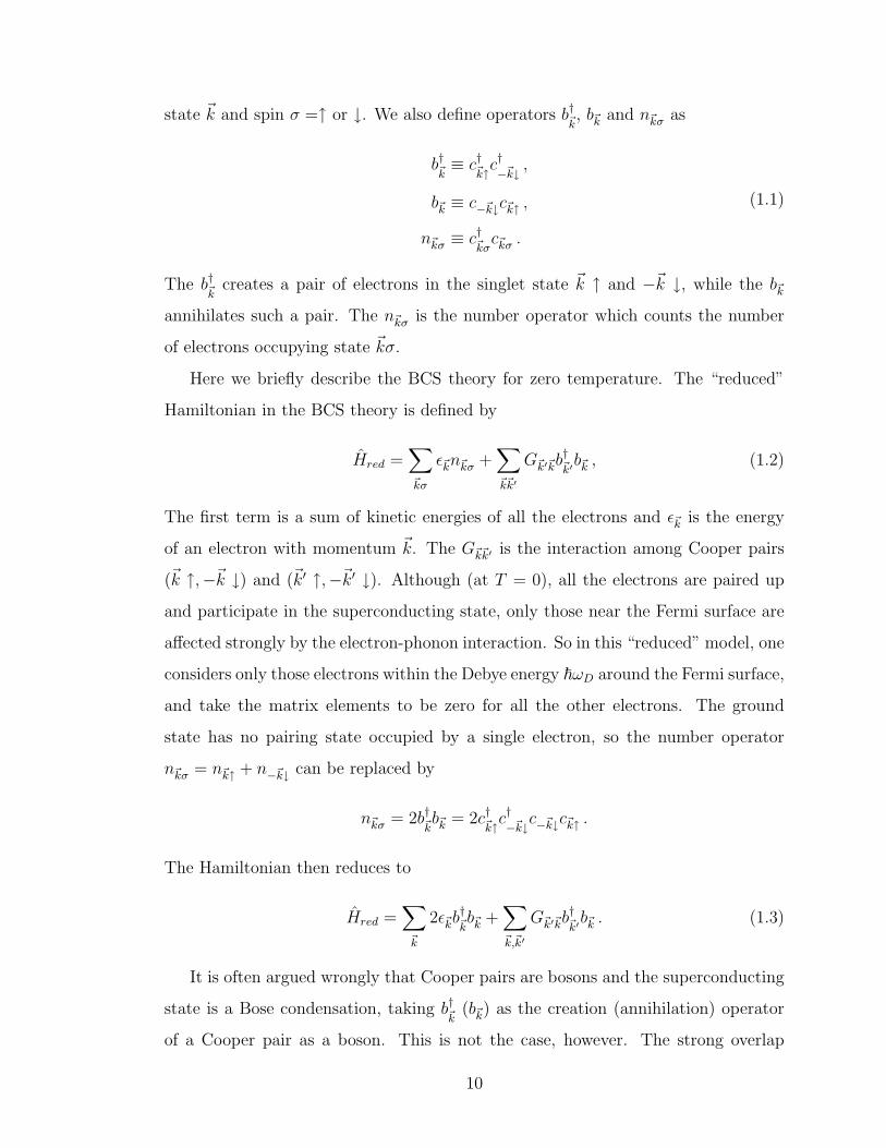
state ~k and spin σ =↑ or ↓. We also define operators b†~k, b~k and n~kσ as

b†~k ≡ c†~k↑c†−~k↓ ,

b~k ≡ c−~k↓c~k↑ ,

n~kσ ≡ c†~kσc~kσ .

(1.1)

The b†~k creates a pair of electrons in the singlet state ~k ↑ and −~k ↓, while the b~k

annihilates such a pair. The n~kσ is the number operator which counts the number

of electrons occupying state ~kσ.

Here we briefly describe the BCS theory for zero temperature. The “reduced”

Hamiltonian in the BCS theory is defined by

Hred =∑

~kσ

ε~kn~kσ +∑

~k~k′

G~k′~kb†~k′

b~k , (1.2)

The first term is a sum of kinetic energies of all the electrons and ε~k is the energy

of an electron with momentum ~k. The G~k~k′ is the interaction among Cooper pairs

(~k ↑,−~k ↓) and (~k′ ↑,−~k′ ↓). Although (at T = 0), all the electrons are paired up

and participate in the superconducting state, only those near the Fermi surface are

affected strongly by the electron-phonon interaction. So in this “reduced” model, one

considers only those electrons within the Debye energy ~ωD around the Fermi surface,

and take the matrix elements to be zero for all the other electrons. The ground

state has no pairing state occupied by a single electron, so the number operator

n~kσ = n~k↑ + n−~k↓ can be replaced by

n~kσ = 2b†~kb~k = 2c†~k↑c†−~k↓c−~k↓c~k↑ .

The Hamiltonian then reduces to

Hred =∑

~k

2ε~kb†~kb~k +

∑

~k,~k′

G~k′~kb†~k′

b~k . (1.3)

It is often argued wrongly that Cooper pairs are bosons and the superconducting

state is a Bose condensation, taking b†~k (b~k) as the creation (annihilation) operator

of a Cooper pair as a boson. This is not the case, however. The strong overlap

10

and correlations among the Cooper pairs play an important role in forming the

superconducting state in a conventional superconductor. The fact that the electrons

are fermions and they satisfy the Pauli exclusion principle is the key factor. It can

also be seen that b~k and b†~k′ above do not satisfy the commutation relations for bosons.

From their definition (1.1), one finds

[b~k , b†~k′ ] = 0 ~k 6= ~k′ ,

[b~k , b†~k′ ] = 1− (n~k↑ + n−~k↓)~k = ~k′ ,

[b~k , b~k′ ] = [b†~k , b†~k′ ] = 0 .

(1.4)

The term n~k↑ + n−~k↓ above is a result of the Pauli exclusion principle acting on the

individual electrons forming a pair. The b~k and b†~k describe pairs of fermions.

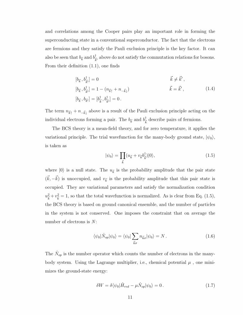
The BCS theory is a mean-field theory, and for zero temperature, it applies the

variational principle. The trial wavefunction for the many-body ground state, |ψ0〉,is taken as

|ψ0〉 =∏

~k

(u~k + v~kb†~k)|0〉, (1.5)

where |0〉 is a null state. The u~k is the probability amplitude that the pair state

(~k,−~k) is unoccupied, and v~k is the probability amplitude that this pair state is

occupied. They are variational parameters and satisfy the normalization condition

u2~k+ v2

~k= 1, so that the total wavefunction is normalized. As is clear from Eq. (1.5),

the BCS theory is based on ground canonical ensemble, and the number of particles

in the system is not conserved. One imposes the constraint that on average the

number of electrons is N :

〈ψ0|Nop|ψ0〉 = 〈ψ0|∑

~kσ

n~kσ|ψ0〉 = N . (1.6)

The Nop is the number operator which counts the number of electrons in the many-

body system. Using the Lagrange multiplier, i.e., chemical potential µ , one mini-

mizes the ground-state energy:

δW = δ〈ψ0|Hred − µNop|ψ0〉 = 0 . (1.7)

11

Substituting the Hamiltonian (1.3) and the wavefunction (1.5) into this equation,

and applying the commutation relations of b†~k and b~k, one has

W =∑

~k

2(ε~k − µ)v2~k

+∑

~k~k′

G~k~k′u~kv~ku~k′v~k′ . (1.8)

Minimizing this energy in terms of u~k and v~k , with the normalization condition, one

obtains

u2~k

=1

2(1 +

ε~k − µ

E~k

) ,

v2~k

=1

2(1− ε~k − µ

E~k

) ,

u~kv~k =∆~k

2E~k

,

(1.9)

where E~k is defined by

E~k ≡[(ε~k − µ)2 + ∆2

~k

]1/2

, (1.10)

and ∆~k satisfy the relation

∆~k = −∑

~k′

G~k~k′∆~k′

2E~k′. (1.11)

The ∆~k is called the pairing potential or the order parameter. One must solve ∆~k

selfconsistently.

When an electron is added to the system in state ~k ↑, or an electron is removed

from state −~k ↓, due to the Pauli exclusion principle, the pair state (~k ↑,−~k ↓) is

not available for Cooper pairs. This results in an increase ∆W in the total energy

of the system,

∆W = ε~k(1− 2v~k)2 − 2

∑

~k′

G~k~k′u~k′v~k′

u~kv~k . (1.12)

Using Eqs. (1.9-1.11), one finds

∆W =ε2~k

E~k

+∆2

~k

E~k

= E~k . (1.13)

In the superconducting state, adding an electron in state ~k ↑ and creating a hole

in −~k ↓ have identical results, both blocking the pair state (~k ↑,−~k ↓) for Cooper

12

pairs, except that the total number of electrons differs by two. Thus, in general, a

single-particle excitation is a superposition of an electron and a hole: this is called

a quasiparticle. The E~k is the energy of a quasiparticle excitation.

One can define the creation and annihilation operators of quasiparticles, γ†~kσand

γ~kσ, respectively [22, 23] as

γ†~k↑ = u~kc†~k↑ − v~kc−~k↓ ,

γ−~k↓ = u?~kc−~k↓ + v?

~kc†~k↑ ,

γ~k↑ = u?~kc~k↑ − v?

~kc†−~k↓ ,

γ†−~k↓ = u~kc†−~k↓ + v~kc~k↑ .

(1.14)

If |ψ0〉 has no quasiparticles, one finds

γ†~k↑|ψ0〉 = |ψ~k↑〉 ,

γ†−~k↓|ψ0〉 = |ψ−~k↓〉 ,

γ~k↑|ψ0〉 = 0 ,

γ−~k↓|ψ0〉 = 0 .

(1.15)

The quasiparticle operators satisfy the Fermi-Dirac statistics:

{γ~kσ , γ†~k′σ′} = δ~k~k′δσσ′ , (1.16)

{γ~kσ , γ~k′σ′} = {γ†~kσ, γ†~k′σ′} = 0 . (1.17)

In general, the order parameter is a function of momentum, reflecting the nature

of the pairing interaction. In an isotropic s-wave superconductor, one can assume

that the interaction strength is independent of momentum, G~k~k′ ≡ G. Then ∆~k

in Eq. (1.13) is a constant, ∆~k ≡ ∆(T ), and ∆(T ) is called the energy gap at

temperature T . As can be seen in Eq. (1.13), it is the minimum energy required

to create a quasiparticle. For such an isotropic case, the excitation energy E~k is

illustrated as a function of momentum magnitude k in Fig. 1.5 [24], in which ∆0 ≡∆(T ).

In the superconducting ground state, there is no single-particle state within the

energy gap, as illustrated in Fig. 1.6 [25]. As the number of states must be conserved,

13

Figure 1.5: Quasiparticle excitation energy as a function of momen-tum k. The kF and EF are the Fermi momentum and Fermi energy,respectively [24].

Figure 1.6: In the superconducting state, energy gap is created aroundE = EF . The ε is the single-particle kinetic energy measured fromEF . The Nn(E) and Ns(E) are the DOS in the normal state andsuperconducting state, respectively [25].

the states inside the gap in the normal state are pushed outside the gap in the

superconducting state. Thus the single-particle density of state (DOS) has a peak

at the gap edge, called the coherence peak, as shown in Fig. 1.6. Experimentally,

one can measure the energy gap and excitation spectrum, for example, by tunneling

electrons or holes into the superconductor. STM can tunnel electrons or holes at

different positions and in different directions. In a homogeneous isotropic system,

the DOS should be independent of position and momentum.

For finite temperature, the BCS theory is formulated on the basis of the statistical

method for a ground canonical ensemble. One of the predictions deducted from the

14

BCS theory that agrees perfectly with experiments, is the temperature dependence

of the energy gap. This is illustrated in Fig. 1.7. The temperature-dependent gap

∆(T ) measured in units of the zero temperature gap ∆0 = ∆(0) is almost unity for

T . 0.4 Tc. As T increases further, it decreases rapidly and continuously to zero

at T = Tc, signaling a second-order phase transition. This behavior is universal for

many different conventional, weak-coupling superconductors (circles in Fig. 1.7), and

agrees very well with the theory.

Figure 1.7: Temperature dependance of measured energy gap for var-ious conventional superconductors. The curve is the BCS prediction[9].

1.3 BdG Theory

The Bogoliubov-de Gennes (BdG) theory [9] is a generalization of the BCS theory,

formulated in real space. The starting point of this theory is to define the creation

and annihilation operators Ψ and Ψ† respectively, in real space:

Ψ(~rσ) =∑

~k

ei~k·~rc~kσ ,

Ψ†(~rσ) =∑

~k

e−i~k·~rc†~kσ.

(1.18)

Here c†~kσand c~kσ are the creation and annihilation operators defined in momentum

space in the BCS theory. The Ψ(~rσ)† (Ψ(~rσ)) creates (removes) an electron with

15

spin σ =↑ or ↓ from position ~r. Assuming a point interaction in real space to describe

s-wave coupling with coupling constant g, the Hamiltonian H can be written as

H = H0 + H1 ,

H0 =

∫d~r

∑σ

Ψ†(~rσ)

[p2

2me

+ U0(~r)

]Ψ(~rσ) ,

H1 = −1

2g

∫d~r

∑

σσ′Ψ†(~rσ)Ψ†(~rσ′)Ψ(~rσ′)Ψ(~rσ) ,

(1.19)

where p is the momentum operator. The H0 above is a sum of the kinetic energy

and single-particle potential energy with the mass of an electron me. The U0(~r)

incorporates crystal potentials and external potentials as due to impurities. The H1

models the electron-phonon interaction among Cooper pairs.

In mean-field approximation, one rewrites the interaction in terms of effective

two-body interactions:

Heff =

∫d~r

[∑σ

Ψ†(~rσ)He(~r)Ψ(~rσ) + U(~r)Ψ†(~rσ)Ψ(~rσ)

+ ∆(~r)Ψ†(~r ↑)Ψ†(~r ↓) + ∆?(~r)Ψ(~r ↓)Ψ(~r ↑)]

, (1.20)

where

He =p2

2me

+ U0(~r)− µ . (1.21)

Here we have introduced the chemical potential µ as in the BCS theory. The U(~r) is

the Hartree-Fock potential arising from the pairing interaction. The last two terms

in Eq. (1.20) are called anomalous terms, representing Cooper pair scattering. It

may be noted that, both of the two terms change the number of particles by two.

The ∆(~r) is the order parameter or the pairing potential, now depending on position

~r.

We diagonalize the effective Hamiltonian

Heff = Eg +∑n,σ

Enγ†nσγnσ , (1.22)

where Eg is the ground state energy. The γ†nσ and γnσ are the creation and annihi-

lation operators of quasiparticle with quantum number n and spin σ, and En is the

16

energy eigenvalue of the quasiparticle excitation. The diagonalization is made via a

unitary transformation,

Ψ†(~r ↑) =∑

n

(u?

nγ†n↑ − vnγn↓

),

Ψ(~r ↓) =∑

n

(v?

nγ†n↑ + unγn↓

).

(1.23)

It is to be noted that, in analogy to Eq. (1.14), the un and vn are the amplitudes of

the electron and hole parts of a quasiparticle with quantum number n, respectively.

Here γnσ and γ†nσ still satisfy the fermion anti-commutation relations, similarly to

Eq. (1.17). Using Eq. (1.22) and the anti-commutation relation of γnσ and γ†nσ, one

has

[Heff , γnσ] = −Enγnσ ,

[Heff , γ†nσ] = Enγ†nσ ,

(1.24)

and

[Ψ(~r ↑), Heff ] = [He + U(r)]Ψ(~r ↑) + ∆(r)Ψ†(~r ↓) ,

[Ψ(~r ↓), Heff ] = [He + U(r)]Ψ(~r ↓)−∆?(r)Ψ†(~r ↑) .(1.25)

From Eqs. (1.23-1.25),[He + U(~r)

]un(~r) + ∆(~r)vn(~r) = Enun(~r) ,

−[H?

e + U(~r)]vn(~r) + ∆?(~r)un(~r) = Envn(~r) .

(1.26)

These are Schrodinger-like equations for the electron and hole amplitudes, u and v, of

a quasiparticle, which are called the BdG equations. The ∆(~r) can be considered as

a pairing potential that couples the electron and hole components. It is important to

realize the difference between ∆(~k) in the BCS theory and ∆(~r) in the BdG theory.

The former is the energy gap to create a quasiparticle excitation in state ~k, while the

latter cannot be considered as the “energy gap”, since it is a function of position.

Nevertheless, ∆(~r) signifies the ordering of the superconductor at position ~r.

By minimizing the free energy, one obtains

U(~r) = −g∑

n

[|un(~r)|2f(En) + |vn(~r)|2(1− f(En))], (1.27)

∆(~r) = +g∑

0≤εn≤~ωD

v?n(~r)un(~r)(1− 2f(En)), (1.28)

17

where f is the Fermi-Dirac distribution function,

f(En) =(e(En−µ)/kBT + 1

)−1, (1.29)

with kB the Boltzmann constant. As in the BCS theory, we assume that the electron-

phonon interaction is nonzero only for the electrons around the Fermi surface within

energy µ±~ωD. Equation (1.28) is called the gap equation. Throughout this work, we

consider isotropic s-wave pairing. In this case, there is no Fock (exchange) interaction

and the Hartree interaction simply shifts the energy levels. Therefore the Hartree-

Fock potential U is neglected in this thesis.

The Eqs. (1.26) and (1.28) must be solved selfconsistently. One starts out solving

Eq. (1.26) by assuming some form of ∆(~r), then construct the new potential from

Eq. (1.28), and then solve Eq. (1.26) with new ∆(~r), and so on. The process is

iterated until selfconsistency is attained. Once selfconsistency is achieved, one can

calculate the LDOS and the tunneling conductance,

A(E,~r) =∑

n

[|un(~r)|2δ(E − En) + |vn(~r)|2δ(E + En)

], (1.30)

∂I(eV, ~r)

∂V∝ −

∑n

[|un(~r)|2f ′(En − eV ) + |vn(~r)|2f ′(En + eV )

], (1.31)

where E and V are the energy and applied bias voltage, respectively. The δ is the

Kronecker delta function. The f ′ is the first derivative of the Fermi-Dirac function.

The BdG equations solve for all the single-particle states. Typically, ~ωD is a few

times the energy gap, and for a weak-coupling superconductor, ~ωD and the energy

gap are of the order of milli-electron-volt, meV. The µ, on the other hand, can be

as large as tens of electron volt (e.g. 12 eV for Al). For such a large µ, solving the

BdG equations exactly and selfconsistently can be a formidable task. In the work for

this thesis, we have solved the BdG equations directly and numerically, by utilizing

parallel computation. The procedure of our parallel computation is discussed in

Appendix A.

18

Chapter 2

Electronic Structure around a Vortex

2.1 Motivation

In this chapter, electronic structure around an isolated vortex in the superconductor

NbSe2 is explored within the framework of the BdG theory. The purpose of this

work is to construct programs for solving the BdG equations selfconsistently for the

well-known problem of a single vortex, and to check that our codes work correctly

by comparison with the results of GS [26] and the experiment [12]. Furthermore, the

local effects of a vortex on superconductivity are expected to be similar to those of a

magnetic impurity in that they both tend to suppress superconductivity locally. So

the work presented in this chapter is a preliminary study to help us better understand

the effects of local magnetic field.

In Sec.2.2, parameter values of NbSe2, for which we investigate the vortex prob-

lem, are explained. In Sec.2.3, our BdG programs are checked for the simplest case,

i.e., for a homogeneous system for which the well-known BCS results are available.

In Sec.2.3, electronic structure around a vortex is studied.

2.2 Material

The calculations are performed for the conventional weak-coupling type-II supercon-

ductor, NbSe2. High-quality single crystals of NbSe2 are readily available, and easy

to cleave for a clean surface ideal for STM. It is the first material from which direct

images of vortex states were obtained [11]. NbSe2 is a layered compound and its

Fermi surface can be well approximated to be a cylinder along the kz direction in

19

momentum space. Thus for the vortex problem, we assume cylindrical symmetry

and solve the problem for a two-dimensional system. Another advantage for BdG

calculation is that its Fermi energy, EF , is relatively small. (Difficulty arising from

large EF is discussed in Section 3.2.2.) The effects of crystal potential U0 can be

incorporated in terms of the effective mass mρ ≡ 2me. ∆0 = 1.2 meV, TC = 8.2 K,

and EF =38.5 meV.

2.3 Homogeneous System

2.3.1 Formulation

In a homogeneous system, the order parameter ∆(~r) is a constant ∆(~r) ≡ ∆. Thus

the BdG equations can be written as

He ∆

∆ −H?e

un(~r)

vn(~r)

= En

un(~r)

vn(~r)

, (2.1)

where

He =p2

2mρ

− EF . (2.2)

For all the results shown in this thesis, we neglect change in the chemical potential

from EF at finite temperature. Assuming cylindrical symmetry, the problem can be

solved in terms of circular cylindrical coordinates (r,θ), and one can separate the

nodal and angular wavefunctions :

un(~r) = uν,l(r)eilθ ,

vn(~r) = vν,l(r)eilθ ,

(2.3)

where ν = 0, 1, 2, · · · is the nodal quantum number and l = 0,±1,±2, · · · is the

angular momentum quantum number. Using Eqs. (2.3), the BdG equations can be

simplified to equations for the radial part of the quasiparticle wavefunctions:

Hr ∆

∆ −H?r

uν,l(r)

vν,l(r)

= Eν,l

uν,l(r)

vν,l(r)

, (2.4)

20

where Hr = − ~22mρ

[1r

ddr

(r d

dr

)− l2

r2

]−EF . We choose the phase of the wavefunctions

so that u(r) and v(r) are real.

In the normal state, ∆ ≡ 0, and the BdG equations reduce to two Schrodinger

equations for a hole and a particle. For a finite system of radius R, the wavefunctions

are,

φm,l(r) =

√2

RJl(αm,l

r

R)/Jl+1(αm,l), (2.5)

which are normalized in a disc of radius R. Here αm,l is the m-th zero of the Bessel

function of order l, Jl (m = 1, 2, · · · ). In the superconducting state, we expand the

quasiparticle amplitudes in terms of the complete orthonormal set of the wavefunc-

tions in the normal state:

uν,l(r) =∑m

cν,mφm,l(r),

vν,l(r) =∑m

dν,mφm,l(r).(2.6)

In a weak-coupling superconductor, only those states close to the Fermi surface are

relevant to superconductivity and the states with energy within ±~ωD (around EF )

are needed in the gap equation. Thus in this expansion, only the states with energies

below EF +ε are included, where ε is of the order of ~ωD. Therefore the node number

m varies from 1 to Nl, where Nl is the maximum node number for a given angular

momentum l, defined by~2α2

Nl,l

2mρR2≤ EF + ε . (2.7)

In our calculation, ε is taken to be 2~ωD. Higher cutoff energy gives the same results.

Substituting Eq. (2.6) into Eqs. (2.1), the BdG equations are reduced to a 2Nl×2Nl

matrix equation for the expansion coefficients for each angular momentum l: T ∆

∆ −T

ψν,l = Eν,lψν,l , (2.8)

where ψTν,l = (cν,1, · · · , cν,Nl

, dν,1, · · · , dν,Nl), and ∆ = ∆I with I the identity matrix.

Due to orthonormality of the Bessel functions, the matrix elements are given by

Tm,m′ = 〈m, l|Hr|m′, l〉

=

(~2α2m,l

2mρ

− EF

)δm,m′ ,

(2.9)

21

and

∆m,m′ = 〈m, l|∆|m′, l〉= ∆δm,m′ .

(2.10)

One solves the eigenvalue problem Eq. (2.8) for all l to obtain states below energy

EF + ε. The order parameter is reconstructed through the gap equation (1.29),

∆(r) = g∑

0≤Eν,l≤~ωD

uν,l(r)vν,l(r)[1− 2f(Eν,l)], (2.11)

where g is the coupling constant. During an iteration, for each angular momentum l,

solving the matrix (2.8) and calculating the contribution to ∆ are a process indepen-

dent of other values of l, and calculation for different values of l can be performed in

parallel. The flow chart of parallel computation is described in Sec. A.2 in Appendix

A. The numerical method for solving the matrix equation is discussed in Sec. A.3.1 .

2.3.2 Results and Discussion

Results for a homogeneous system of clean NbSe2 are presented for R = 10, 000 a.u..

For programming, we use the boundary radius R (in units of a.u. which is 0.5292 A)

and the bulk zero-temperature energy gap ∆0 = 1.2 meV as the length and energy

unit, respectively. The coupling constant g is about 3 meV·A for R = 10, 000 a.u.

and ~ωD is taken to be 3 meV, which yields Tc ≈ 8.2 K.

Figure 2.1 shows the tunneling conductance dI/dV of a pure NbSe2 sample as

a function of voltage V for temperature T = 1 K, 2 K, 5 K, and 7 K. We have

confirmed that both dI/dV and LDOS are independent of position r, as expected

for a homogeneous system. We have performed calculation for T =0.1 K and have

found that the result is almost the same as for T =1 K. In Fig. 2.1, the existence of

the energy gap ∆ ≡ ∆(T ) around the Fermi surface eV/∆0 = 0 and the coherence

peak at eV/∆0± 1, can be seen clearly. As temperature is increased, more and more

quasiparticles are created (for a given voltage), which results in a smaller energy gap.

Accordingly, more states are created inside ∆0 and thus the coherence peak height is

reduced. As T reaches Tc = 8.2 K, superconductivity is destroyed totally, the energy

22

gap ceases to exist and the density of states (LDOS and dI/dV ) becomes flat as a

function of energy. Note that in a free electron gas in two dimensions (in the normal

state), the bulk DOS is a constant.

0

1

2

−3 −2 −1 0 1 2 3

dI(e

V,r

)/dV

eV/∆0

Clean NbSe2 : Tunneling Conductance

T = 1KT = 2KT = 5KT = 7K

Figure 2.1: Normalized tunneling conductance of a pure NbSe2 attemperature T = 1 K, 2 K, 5 K and 7 K.

The LDOS for the homogeneous system is shown in Fig. 2.2. Here for presentation

purpose each delta function in Eq. (1.30) has been replaced by a normalized Gaussian

of width γ,

δ(eV ± En) =1

γ√

πexp

[−

(eV± En

γ

)2], (2.12)

with γ = 0.1. For T = 1 K and 2 K, the LDOS is identical. Apparently, the

energy gap decreases rather slowly as temperature is reduced, for T . 5 K. To see

the temperature dependance more clearly, we show in Fig. 2.3 the uniform order

parameter ∆(T ) as a function of temperature T . The smooth, slow decrease of the

gap as T increases can be seen: ∆ reaches a half of ∆0 at T ≈ 7.5 K and the gap

closes rapidly as T approaches to Tc. This behavior is consistent with the BCS theory

shown in Fig. 1.7. The BCS theory gives an analytical formula for ∆ as a function

of T for T ≈ TC [27] as

∆(T ) ≈ 1.74∆0

√1− T

TC

. (2.13)

23

0

1

2

−3 −2 −1 0 1 2 3

Nor

mal

ized

A(e

V,r

)

eV/∆0

Homogeneous NbSe2 : Density of States

T = 1KT = 2KT = 5KT = 7K

Figure 2.2: LDOS of a pure NbSe2 at temperature T = 1 K, 2 K, 5K and 7 K.

Our result yields this behavior as indicated in Fig. 2.3, where the BCS formula above

is plotted in the dashed curve.

2.4 Isolated Vortex

2.4.1 Formulation

The BdG equations in the presence of magnetic field are

He ∆(~r)

∆?(~r) −H?e

un(~r)

vn(~r)

= En

un(~r)

vn(~r)

, (2.14)

with the single-particle Hamiltonian

He =1

2mρ

(p− e

c~A(~r)

)2

− EF ,

where ~A(~r) is the vector potential. The He depends on the choice of ~A, which is not

unique. However, under a gauge transformation,

~A′ = ~A +∇χ(~r), (2.15)

24

0 2 4 6 8

T (K)

0

0.2

0.4

0.6

0.8

1

Δ/Δ₀

Δ/Δ₀ = 1.74(T-T/T )

Homogeneous NbSe₂ : Energy Gap

c1/2

Figure 2.3: Uniform order parameter ∆ as a function of temperature.

all physical observables must be invariant. The quasiparticle wavefunctions are trans-

formed by such a gauge transformation to u′n(~r)

v′n(~r)

=

un(~r)exp[ ie

~cχ]

vn(~r)exp[− ie~cχ]

, (2.16)

and the order parameter changes to

∆′(~r) = ∆(~r)e2ie~c χ(~r) . (2.17)

One can show that u′n, v′n, and ∆′ satisfy the BdG equations of the same form as

Eq. (2.14), and thus the quasiparticle eigenvalues are gauge invariant. The self-

consistent pairing potential ∆(~r) must be a single-valued function of ~r, no matter

what gauge one takes. For example, in a cylindrically symmetric system, the gauge

function must be of the form

χ =~c2e

mθ, (2.18)

where θ is the azimuthal angle in two-dimensional polar coordinates, and m is an

integer.

Consider an isolated vortex passing through r = 0 along the z direction. To

model NbSe2, we assume cylindrical symmetry and isotropic s-wave pairing. It is

25

convenient to choose a gauge so that

∆(~r) = |∆(r)|e−iθ. (2.19)

One can eliminate the phase with a gauge transformation with

χ =~c2e

θ. (2.20)

Thus the new pairing potential is

∆′(~r) = |∆(r)|. (2.21)

The flux quantization, namely the fact that a vortex encloses a quantum of mag-

netic flux, φ0 = hc2e

, is a direct consequence of the single-valuedness of the pairing

potential, which corresponds to the Cooper-pair wavefunction in the GL theory. The

flux quantization has been confirmed experimentally [28, 29, 30]. In general, a vor-

tex can carry multiple flux quanta. In the vortex lattice in a bulk system, however,

the most energetically favorable state is such that each vortex carries only one flux

quantum [15]. Recently, vortices carrying multiple flux quanta have been observed in

mesoscopic superconductors, in which the system size is comparable to the coherence

length [31, 32, 33, 34, 15].

NbSe2 is strongly type-II with κ ≈ 10 (λ ≈ 1400 A, ξ ≈ 140 A) [35, 36, 37], and

one can assume that the magnetic field around a vortex is constant. Thus in our

BdG equations, we ignore the vector potential, and the equations are

He ∆(r)

∆?(r) −H?e

un(~r)

vn(~r)

= En

un(~r)

vn(~r)

, (2.22)

where He = − ~22mρ

[1r

∂∂r

(r ∂

∂r

)+ 1

r2∂2

∂θ2

]− EF . The angular momentum l is a good

quantum number under cylindrical symmetry, so one can separate the wavefunctions

into the radial and angular parts,

un(~r)

vn(~r)

=

uν,l(r)e

i(l− 12)θ

vν,l(r)ei(l+ 1

2)θ

, (2.23)

26

where l = ±12,±3

2,±5

2, · · · . Using Eqs. (2.23), the BdG equations can be simplified

to equations for the radial part of the quasiparticle wavefunctions:

H−

r |∆(r)||∆(r)| −H+

r

uν,l(r)

vν,l(r)

= Eν,l

uν,l(r)

vν,l(r)

, (2.24)

where H±r = − ~2

2mρ

[1r

ddr

(r d

dr

)− (l±1/2)2

r2

]−EF . The following steps to deal with the

BdG equations are similar to those used in the homogeneous problem. We expand

the radial part of the quasiparticle amplitudes, un(r) and vn(r), in terms of the

complete orthonormal set of the Bessel functions which are normalized in a disc of

radius R:

uν,l(r) =∑

k

cν,kφk,l−1/2(r),

vν,l(r) =∑

k

dν,kφk,l+1/2(r),(2.25)

where φk,l′(r) =√

2R

Jl′(αk,l′rR)/Jl′+1(αk,l′) with l′ = l ± 1

2an integer. Only the states

below the cutoff energy EF + 2~ωD are included in our calculation (higher cutoff

energy gives the same results), and the cutoff energy determines the maximum l

and Nl. By substituting Eq. (2.25) into Eq. (2.24), we have a matrix equation of

dimension 2Nl × 2Nl for each angular momentum l:

T− ∆

∆T −T+

ψν,l = Eν,lψν,l, (2.26)

where ψTν,l = (cν,1, ..., cν,Nl

, dν,1, ..., dν,Nl). Due to orthonormality of the Bessel func-

tions, the matrix elements are reduced to

T−k,k′ = 〈k, l − 1

2|H−

r |k′, l −1

2〉

=

(~2α2k,l− 1

2

2mρ

− EF

)δk,k′ ,

T+k,k′ = 〈k, l +

1

2|H+

r |k′, l +1

2〉

=

(EF −

~2α2k,l+ 1

2

2mρ

)δk,k′ ,

(2.27)

27

and

∆k,k′ = 〈k, l − 1

2|∆(r)|k′, l +

1

2〉

=

∫ ∞

0

r drφk,l− 12(r)|∆(r)|φk′,l+ 1

2(r).

(2.28)

The BdG equations are invariant under the transformation,

uν,l(~r) −→ v?ν,−l(~r),

vν,l(~r) −→ −u?ν,−l(~r),

Eν,l −→ −Eν,−l.

(2.29)

In our system, this means that a positive-energy state for negative angular momen-

tum −l and energy Eν,−l is equivalent to the negative-energy state for positive l and

energy Eν,l = −Eν,−l. Therefore, one can cut the computational time almost by half

by obtaining positive- and negative-energy solutions for positive l only.

As in the homogeneous case, we perform calculation according to the flow chart in

Fig A.4 in Sec. A.2 in Appendix A, until selfconsistency is achieved. The numerical

procedure for evaluation of the matrix elements is discussed in Sec. A.3.2 . The order

parameter is calculated at a discrete set of positions, while calculation of the matrix

elements in Eq. (2.28) requires ∆(r) as a smooth function of r. So curve fitting,

which is described in Appendix B, is applied.

2.4.2 Results and Discussion

We present results for the same parameter values as for the homogeneous case.

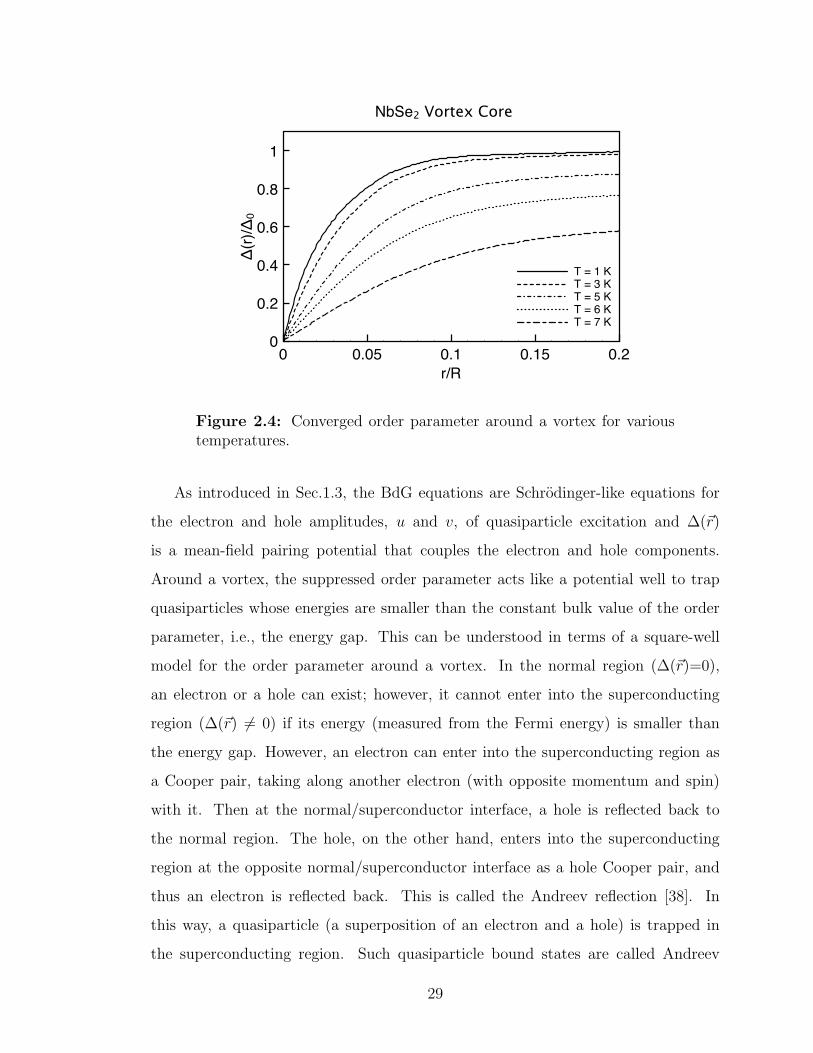
Figure 2.4 shows the converged order parameter ∆(r) as a function of radial co-

ordinate r for various temperatures. It can be seen that the order parameter is

suppressed to zero at the center of the vortex and gradually recovers to the bulk

value as r increases. In the macroscopic picture of the GL theory, ∆(~r) corresponds

to the Cooper pair wavefunction. The spatial distribution of the order parameter in-

dicates that Cooper pairs are broken up and superconductivity is suppressed around

a vortex. The length scale over which the order parameter recovers to the bulk value

is a few times the coherence length (roughly, the size of a Cooper pair).

28

0 0.05 0.1 0.15 0.2

r/R

0

0.2

0.4

0.6

0.8

1

Δ(r)/Δ₀

T = 1 KT = 3 KT = 5 KT = 6 KT = 7 K

NbSe₂ Vortex Core

Figure 2.4: Converged order parameter around a vortex for varioustemperatures.

As introduced in Sec.1.3, the BdG equations are Schrodinger-like equations for

the electron and hole amplitudes, u and v, of quasiparticle excitation and ∆(~r)

is a mean-field pairing potential that couples the electron and hole components.

Around a vortex, the suppressed order parameter acts like a potential well to trap

quasiparticles whose energies are smaller than the constant bulk value of the order

parameter, i.e., the energy gap. This can be understood in terms of a square-well

model for the order parameter around a vortex. In the normal region (∆(~r)=0),

an electron or a hole can exist; however, it cannot enter into the superconducting

region (∆(~r) 6= 0) if its energy (measured from the Fermi energy) is smaller than

the energy gap. However, an electron can enter into the superconducting region as

a Cooper pair, taking along another electron (with opposite momentum and spin)

with it. Then at the normal/superconductor interface, a hole is reflected back to

the normal region. The hole, on the other hand, enters into the superconducting

region at the opposite normal/superconductor interface as a hole Cooper pair, and

thus an electron is reflected back. This is called the Andreev reflection [38]. In

this way, a quasiparticle (a superposition of an electron and a hole) is trapped in

the superconducting region. Such quasiparticle bound states are called Andreev

29

bound states [13, 14]. Similarly to the potential well problem in the normal state,

such bound states exist with discrete energy levels, for which the electron and hole

amplitudes interfere constructively.

For low temperature T . 2 K, the order parameter and the LDOS ( dIdV

) are

insensitive to temperature. We calculated the order parameter for T = 0.1 K and

found it was almost the same as that for T = 1 K. For temperature T & 3 K, as

can be seen in Fig. 2.4, the order parameter is overall decreased with increasing tem-

perature. The temperature dependence of the bulk value is consistent with Fig. 2.3.

Temperature affects not only the value of the energy gap (the bulk order parameter),

but also the radius of the “vortex core”. The size of the vortex core decreases with

decreasing temperature as can be seen in Fig. 2.4. The temperature dependence can

be characterized by the vortex core size defined by [39]

ξ−1c = lim

r→0

∆(r)

r

1

∆(r = ∞). (2.30)

As temperature is decreased, the slope of the order parameter at r = 0 increases

and thus the core size decreases. In the limit of zero temperature, the slope diverges

and the vortex core area shrinks to zero. This is called the Kramer-Pesch effect [39],

and it stems from thermal depopulation of quasiparticle bound states in the core.

When temperature decreases, the number of quasiparticles bound in the potential

well decreases, which relieves suppression of the order parameter.

In Fig. 2.5, the energy eigenvalues are plotted as a function of angular momentum

l for T = 1 K. It can be seen that a bound state branch (one bound state for each

angular momentum that is smaller than a certain value) exists inside the energy gap.

The bound state energy is almost zero for l = 1/2, and it approaches towards the

gap edge as |l| increases. The quantization (and the degeneracy) of energy levels

in the scattering states is a finite-size effect due to finite radius R. However, the

stronger quantization for small l, as can be seen in this figure, is due to resonance in

the “potential well” region.

In Fig. 2.6, the electron and hole amplitudes of the lowest-energy bound state

(l = 1/2) are shown (T = 1 K). It can be seen that the quasiparticle is confined in

30

-200 -100 0 100 200

Angular momentum

-2

-1

0

1

2

Eigenvalues

NbSe₂ Vortex State

Figure 2.5: Energy levels of quasiparticle states as a function of an-gular momentum l.

the vortex core region, decaying rapidly for r & 0.1R. It can also be seen that there

is a phase shift between the electron and hole amplitudes. This is in contrast to the

wavefunctions of scattering states, as illustrated in Fig. 2.7 for l = 1/2. One can see

that in this case the wavefunction is extended outside the vortex core. As this is the

lowest-energy scattering state, there is still a phase shift between the electron and

hole amplitudes; however, the shift is only in the vortex core region.

Figure 2.8 shows the calculated dI/dV as a function of energy eV and radial dis-

tance r for T = 1 K. At r = 0, we can see the zero-energy bound state corresponding

to l = 1/2. As one moves away from the vortex center, the bound state branches

of positive energy (positive l) and negative energy (negative l) show up, merging

finally to the gap edge, corresponding to large l. Far away from the vortex core, a

coherence peak develops at the gap edge and the BCS DOS (dI/dV ) is recovered.

It is interesting to note that the “recovery length” over which the LDOS (dI/dV )

recovers to the bulk behavior is substantially larger than that of the order parameter

(see Fig. 2.4). The decay of the zero-bias peak as a function of r is consistent with

that of the wavefunctions shown in Fig. 2.6.

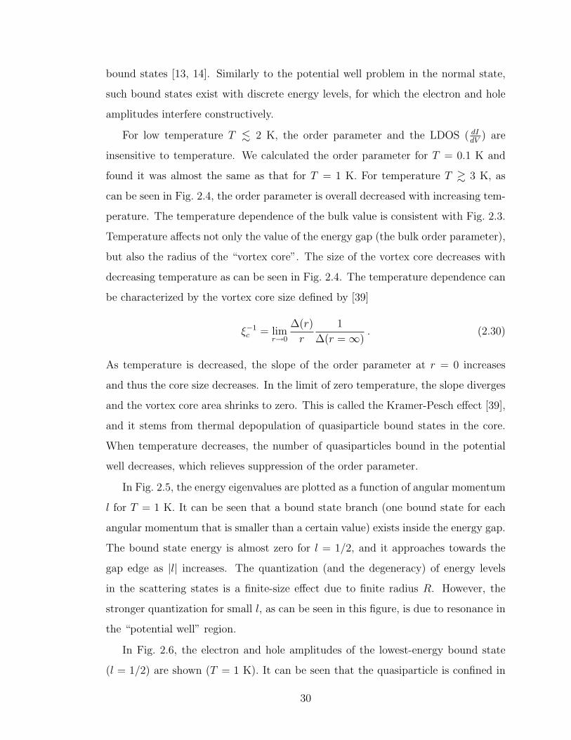
The splitting of the zero-bias bound state peak for nonzero r can be seen clearly

in the slices of dI/dV at various r shown in Fig. 2.9. It can be seen in this figure

that at r = 2000 a.u. (r/R = 0.2) the bound state peak has almost merged to the

31

0

0 0.1 0.2

Wav

e F

unct

ion

(arb

. uni

t)

r/R

NbSe2 Vortex State: E1,1/2 = 0.001

u(r)v(r)

Figure 2.6: Electron and hole amplitudes of the quasiparticle boundstate around a vortex for l = 1/2 and T = 1 K.

gap edge, where the coherence peak has started developing. However, this is still not

quite the BCS behavior and one must go further away to recover the BCS DOS. The

small oscillations for energies larger than the energy gap are due to the quantization

of the energy levels described earlier.

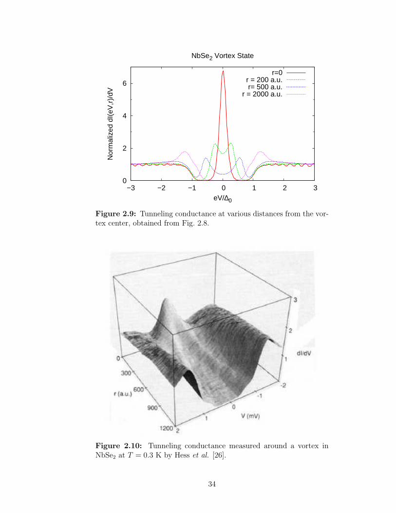
Quasiparticle excitations around the vortex can be probed by tunneling an elec-

tron or a hole into the vortex core region by STM. In Fig. 2.10, the measured dI/dV

as a function of radial distance and applied voltage at T = 0.3 K is shown. We can

see that our result, Fig. 2.8, is consistent with the observation. In actual experi-

ment, there are nonmagnetic impurities and defects in samples. They, along with

finite temperature, tend to make dI/dV smeared compared with theoretical calcu-

lation. The excellent agreement with the experiment justifies our approximation

of neglecting the spatial variation of magnetic field around a vortex. Our results

are also consistent with those of GS [26] and it confirms the accuracy of our BdG

program.

32

0

0 0.1 0.2

Wav

e F

unct

ion

(arb

. uni

t)

r/R

NbSe2 Vortex State: E2,1/2=1.007

u(r)v(r)

Figure 2.7: Electron and hole amplitudes of the lowest-energy scat-tering state around a vortex.

NbSe2 Vortex State

−3−2−1 0 1 2 3

eV/∆0

0

0.1

0.2

r/R

01234567

dI(eV,r)/dV

Figure 2.8: Tunneling conductance around a vortex for T = 1 K.

33

0

2

4

6

−3 −2 −1 0 1 2 3

Nor

mal

ized

dI(

eV,r

)/dV

eV/∆0

NbSe2 Vortex State

r=0r = 200 a.u.r= 500 a.u.

r = 2000 a.u.

Figure 2.9: Tunneling conductance at various distances from the vor-tex center, obtained from Fig. 2.8.

Figure 2.10: Tunneling conductance measured around a vortex inNbSe2 at T = 0.3 K by Hess et al. [26].

34

Chapter 3

Electronic Structure around a Magnetic

Impurity

In this chapter, electronic structure around an isolated magnetic impurity in an

s-wave superconductor is examined within the framework of the BdG theory. The

aim is to understand the pair-breaking nature of a magnetic impurity and the ex-

perimental observation of Ref. [20]. Magnetic impurity atoms tend to have the spins

of neighboring electrons aligned or anti-aligned with their spin to form a net local

magnetic moment, so that original Cooper pairs (~k ↑,−~k ↓) are broken and thus

superconductivity is suppressed locally. Similarly to a vortex, such a local magnetic

moment results in inhomogeneous order parameter. Like the vortex problem, such

inhomogeneity effects should be studied by solving the BdG equations selfconsis-

tently. We model the interaction between the magnetic atom and the conduction

electrons by a coupling of classical spins (i.e., we ignore dynamical effects) over the

length scale of a few atomic distances. We assume that the spin potential created

by the magnetic atom is spherical and solve the BdG equations in three-dimensional

spherical coordinates.

In Sec.3.1, to check the three-dimensional program, the problem of a homoge-

neous superconductor is solved. In Sec.3.2, by assuming the spin potential to have

a Gaussian form, we investigate the effects of a magnetic impurity.

35

3.1 Homogeneous System

3.1.1 Formulation

As discussed in the Sec.2.3, the order parameter ∆(~r) = ∆(r) ≡ ∆ is a constant

in a homegenous system. With spherical symmetry, radial and angular coordinates,

(r, θ, φ), of the quasiparticle wavefunctions can be separated as

un(~r) = uν,l(r)Yl,m(θ, φ) ,

vn(~r) = vν,l(r)Yl,m(θ, φ) ,(3.1)

where {Yl,m; l = 0, 1, 2, · · · ; m = −l, · · · , l} are the spherical harmonics:

Yl,m(θ, φ) = (−1)m

√2l + 1

4π

(l −m)!

(l + m)!Pm

l (cosθ)eimφ . (3.2)

The ν above is the nodal quantum number (ν = 1,2,· · · ). Using Eqs. (3.1), the BdG

equations can be reduced to

Hr ∆

∆ −H?r

uν,l(r)

vν,l(r)

= Eν,l

uν,l(r)

vν,l(r)

, (3.3)

where Hr = − ~22m

[d2

dr2 + 2r

ddr

+ l(l+1)r2

]− EF . Analogously to the method for the

vortex problem, the radial wavefunctions can be expanded in terms of the complete

orthonormal set of the spherical Bessel functions:

uν,l(r) =∑

k

cν,kρk,l(r) ,

vν,l(r) =∑

k

dν,kρk,l(r) ,(3.4)

where

ρk,l(r) =

√2√R3

jl(αk,lr

R)/jl+1(αk,l)

=

√2

R√

rJl+ 1

2(αk,l

r

R)/Jl+ 3

2(αk,l) .

(3.5)

36

Here the spherical Bessel functions of order l, jl(αk,lrR), are normalized in a sphere

of radius R and αk,l is the k-th zero of jl. The Jl+ 12

is the cylindrical Bessel function

with a fractional order l + 12:

jl(x) =

√π

2xJl+ 1

2(x).

As in the vortex problem, in a weak-coupling superconductor, only those states close

to the Fermi surface are relevant to superconductivity. We consider only the states

with energy below EF + ε, where ε is of the order of ~ωD. The maximum nodal

quantum number Nl for a given l is determined by

~2α2Nll

2mR2≤ EF + ε. (3.6)

Substituting Eq. (3.4) into Eq. (3.3), we obtain a 2Nl × 2Nl matrix equation for the

expansion coefficients for each angular momentum l:

T ∆

∆ −T

ψν,l = Eν,lψν,l , (3.7)

where ψTν,l = (ck,1, · · · , ck,Nl

, dk1, · · · , dkNl). The equation has 2Nl sets of eigenvalues

Eν and eigenvectors ψν . Due to orthonormality of the Bessel functions, matrix

elements of the Hamiltonian are given by

Tk,k′ = 〈k, l|Hr|k′, l〉

=

(~2α2k,l

2m− EF

)δk,k′

(3.8)

and

∆k,k′ = 〈k, l|∆|k′, l〉 = ∆δk,k′ . (3.9)

In the gap equation,

∆(~r) = g∑

0≤Eν,l,m≤~ωD

uν,l,m(~r)v?ν,l,m(~r)[1− 2f(Eν,l,m)], (3.10)

the summation is over the three quantum numbers, n = (ν, l, m). The order parame-

ter in a spherically symmetric system should be a function of radial coordinate only.

37

One can see this by substituting Eq. (3.1) into Eq. (3.10) and using the following

property of the spherical harmonics [40].

l∑

m=−l

Yl,mY ?l,m ∝ 2l + 1 .

Thus

∆(~r) ∝ g∑

0≤Eν,l≤~ωD

uν,l(r)vν,l(r)?

[1− 2f(Eν,l)

](2l + 1).

Similarly, we have:

A(~r, E) ∝∑

ν,l

[|uν,l(r)|2δ(E − Eν,l) + |vν,l(r)|2δ(E + Eν,l)](2l + 1), (3.11)

∂I(~r, V )

∂V∝ −

∑

ν,l

[|uν,l(r)|2f ′(Eν,l − eV ) + |vν,l(r)|2f ′(Eν,l + eV )](2l + 1). (3.12)

3.1.2 Results and Discussion

The program for the three-dimensional BdG equations has first been applied to the

homogeneous problem. In Fig. 3.1, the tunneling conductance, dI/dV for clean

Nb for T = 1 K is shown. For Nb, EF = 950 meV, the zero-temperature gap

∆0 =1.45 meV, ~ωD =23.86 meV, and Tc=9.2 K. The result shown is for the system

size R =15,000 a.u.. The LDOS (e.g., with smoothing width γ=0.1) looks very

similar to dI/dV . As can be seen in Fig. 3.1, dI/dV clearly shows the energy gap

and the coherence peak, and as expected, it is independent of position r. The

oscillations in dI/dV outside the energy gap are a finite-size effect due to finite R.

In three dimensions, quantization of the energy levels is more pronounced than in

two dimensions presented in Chapter 2.

3.2 Isolated Magnetic Impurity

3.2.1 Formulation

The problem of magnetic exchange interactions between a magnetic impurity atom

and the conduction electrons is very complex. There are several models with different

38

0

1

2

−3 −2 −1 0 1 2 3

Nor

mal

ized

dI(

eV,r

)/dV

eV / ∆0

Clean Nb: Tunneling Conductance

Figure 3.1: Tunneling conductance of a pure Nb at temperature T=1K.

levels of approximations to deal with this problem. One method [41] assumes the

exchange interaction to be isotropic, taking into account of screening effects of the

Coulomb interaction. The Hamiltonian can be written as

Hat = −2Jat~S · ~s ,

where ~S is the spin of the magnetic impurity and ~s is the conduction electron spin

at the position of the magnetic impurity. The Jat signifies the coupling strength

between the spins and it is always positive [41]. At this level, we neglect effects of

the covalent mixing which means that local orbitals of the magnetic impurity form

covalent bonds with the conduction electrons. To incorporate the covalent mixing

into the equation above, Schrieffer and Wolff [42] have shown that Jat should be

replaced with a generalized J , where

H = −2J ~S · ~s ,

and

J = Jat + Jcm .

The Jcm represents the strength of covalent mixing and it can be positive or negative,

depending on the orbital nature of the conduction electrons [43]. Weights of the two

39

components determine the sign of J . The magnetic impurity with J > 0 (J < 0)

is ferromagnetic (antiferromagnetic). Mn and Gd, the two magnetic atoms used in

the experiment of Yazdani et al., are common choices for studying their magnetic

properties experimentally. Both of them can be ferromagnetic or antiferromagnetic

depending on the host. For Mn, Jcm is usually negative and even dominates Jat [41].

But exceptions still exist. For example, J is positive in MgB2 [44]. For Gd, J is

positive in the superconducting materials La and LaAl2 [45], and it is negative in

another superconducting material LaOs2 [43].

In the model above, dynamical effects of magnetic interactions can be included

by introducing an additional field at the impurity site [43]. However, in a fully-

gapped s-wave superconductor, we can assume the spin of the magnetic impurity to

be classical and static [20, 46]. Therefore, in our work, we introduce a spin-dependent

static potential provided by the magnetic impurity to model its spin effects on the

conduction electrons. The effective Hamiltonian Eq. (1.20) is generalized as

Heff =

∫d~r

[Ψ†↑(~r)He(~r)Ψ↑(~r) + Ψ†

↓(~r)He(~r)Ψ↓(~r)

− Uspin(~r)Ψ†↑(~r)Ψ↑(~r) + Uspin(~r)Ψ†

↓(~r)Ψ↓(~r)

+ ∆(~r)Ψ†↑(~r)Ψ

†↓(~r) + ∆?(~r)Ψ↓(~r)Ψ↑(~r)

]. (3.13)

The third and the fourth terms are the potential energies of spin-up and spin-down

electrons, respectively. Furthermore, this potential is assumed to be spherically

symmetric and of a Gaussian form,

Uspin(~r) ≡ Vsexp

[−

(r

λ

)2], (3.14)

where λ is a length scale of the spin potential and Vs represents the coupling strength.

This is a good approximation for Mn, which has three valence electrons. When Vs > 0

(Vs < 0), the coupling is ferromagnetic (antiferromagnetic). Assuming the coupling

is ferromagnetic, this potential decreases the energy of an electron with spin up (a

hole with spin down) and increases that of an electron with spin down (a hole with

40

spin up). Starting from this effective Hamiltonian, we can derive the BdG equations:

He − Uspin ∆(~r)

∆(~r) −H?e − Uspin

un,↑(~r)

vn,↓(~r)

= En↑

un,↑(~r)

vn,↓(~r)

, (3.15)

and He + Uspin ∆(~r)

∆(~r) −H?e + Uspin

un,↓(~r)

vn,↑(~r)

= En↓

un,↓(~r)

vn,↑(~r)

. (3.16)

If the coupling is antiferromagnetic, the sign of Uspin is reversed; however, the com-

bination of the two BdG equations above give the same result as for ferromagnetic

coupling. A spin-up (-down) bound state is a superposition of a spin-up (-down)

electron and a spin-down (-up) hole. One can obtain the results of the equations for

spin-down states Eq. (3.16) from those for spin-up states Eq. (3.15), by the trans-

formation,

un↑ = −vn↑ ,

vn↓ = un↓ ,

En↑ = −En↓ .

(3.17)

Therefore, we only have to solve Eq. (3.15) for positive- and negative-energy states,

and obtain the solutions of Eq. (3.16) through these relations.

As in the homogeneous problem, the quasiparticle wavefunctions can be taken

apart into radial and angular parts. The radial BdG equations are

Hr − Uspin ∆(r)

∆(r) −H?r − Uspin

uν,l,↑(r)

vν,l,↓(r)

= Eν,l, ↑

uν,l,↑(r)

vν,l,↓(r)

, (3.18)

where Hr = − ~22m

[d2

dr2 + 2r

ddr

+ l(l+1)r2

]− EF . Here the pairing potential ∆ is only a

function of distance r due to the spherical symmetry of the impurity potential. As

before, we expand the radial wavefunctions in terms of the complete orthonormal

set of the spherical Bessel functions {jl(x)}. For relatively strong spin potential,

states far away from the Fermi surface can be affected. Thus much more states

are included in the gap equation compared with the vortex problem. The matrix

41

equation for each l is

T − U ∆

∆ −T − U

ψν,l ,↑ = Eν,l ,↑ψν,l ,↑ , (3.19)

where ψTν,l ,↑ = (ck,1, · · · , ck,Nl

, dk,1, ..., dk,Nl), and

Tk,k′ = 〈k, l|Hr|k′, l〉

=

(~2α2k,l

2m− EF

)δk,k′ ,

∆k,k′ = 〈k, l|∆(r)|k′, l〉

=

∫ ∞

0

ρk,l(r)∆(r)ρk′,l(r)r2dr

Uk,k′ = 〈k, l|U(r)|k′, l〉

= Vs

∫ ∞

0

r2ρk,l(r)ρk′,l(r)exp

[−

(r

λ

)2]dr.

(3.20)

Here again we utilize parallel computation, following the flow chart in Fig. A.4 and

assigning different sets of l values to different nodes. The numerical procedure is

discussed in Sec. A.3.4 . As in the vortex problem, curve fitting (Appendix B) is

used for evaluation of the matrix elements.

3.2.2 Results and Discussion

As discussed in the Appendix, the major difficulty in computation for Nb exists in the

integration of matrix elements 〈k, l|∆(r)|k′, l〉. The larger the nodal number k, the

more oscillations the Bessel functions have, and this makes the numerical calculation

challenging. The maximum nodal number Nl is determined by Eq. (2.7), namely,

N2l ∝ (EF + ε)R2. Due to very large EF (≈ 950 meV) for Nb, we have been able to

solve the BdG equations for R ≤ 3, 000 a.u. . However, we have another numerical

problem in this case. The difference between two neighboring energies for a given l,

Eν,l and Eν+1,l, can be roughly estimated by

42

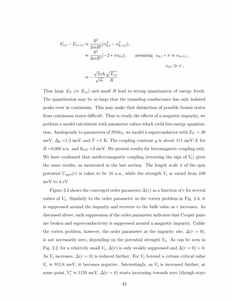
Eν,l − Eν+1,l ≈ ~2

2mR2(α2

k,l − α2k+1,l),

≈ ~2

2mR2(−2 ∗ παk,l), assuming αk,l + π ≈ αk+1,l ,

αk,l À π ,

≈ −√

2π~√m

√Eν,l

R.

Thus large EF (≈ Eν,l) and small R lead to strong quantization of energy levels.

The quantization may be so large that the tunneling conductance has only isolated

peaks even in continuum. This may make that distinction of possible bound states

from continuum states difficult. Thus to study the effects of a magnetic impurity, we

perform a model calculation with parameter values which yield less energy quantiza-

tion. Analogously to parameters of NbSe2, we model a superconductor with EF = 40

meV, ∆0 =1.2 meV and T =1 K. The coupling constant g is about 111 meV·A for

R =8,000 a.u. and ~ωD =3 meV. We present results for ferromagnetic coupling only.

We have confirmed that antiferromagnetic coupling (reversing the sign of Vs) gives

the same results, as mentioned in the last section. The length scale λ of the spin

potential Uspin(r) is taken to be 10 a.u., while the strength Vs is varied from 100

meV to 4 eV.

Figure 3.2 shows the converged order parameter ∆(r) as a function of r for several

values of Vs. Similarly to the order parameter in the vortex problem in Fig. 2.4, it

is suppressed around the impurity and recovers to the bulk value as r increases. As

discussed above, such suppression of the order parameter indicates that Cooper pairs

are broken and superconductivity is suppressed around a magnetic impurity. Unlike

the vortex problem, however, the order parameter at the impurity site, ∆(r = 0),

is not necessarily zero, depending on the potential strength Vs. As can be seen in

Fig. 3.2, for a relatively small Vs, ∆(r) is only weakly suppressed and ∆(r = 0) > 0.

As Vs increases, ∆(r = 0) is reduced further. For Vs beyond a certain critical value

Vc ≈ 915.8 meV, it becomes negative. Interestingly, as Vs is increased further, at

some point, V ′c ≈ 1150 meV, ∆(r = 0) starts increasing towards zero (though stays

43

−0.4

0

0.4

0.8

1.2

0 0.005 0.01 0.015 0.02 0.025

∆(r)

/ ∆ 0

r/R

Model system: order parameter

Vs=600meV.Vs=916meV

Vs=1200meV

Figure 3.2: Order parameter around a magnetic impurity for differentstrengths of the spin potential.

negative). This behavior is illustrated in Fig. 3.3, where ∆(r = 0) (red solid curve)

and |∆(r = 0)| (green dashed curve) are plotted as a function of Vs. As mentioned

before, ∆(r) corresponds to the Copper pair wavefunction in the macroscopic picture.

The |∆(r = 0)| signifies the strength of superconductivity at r = 0. It can be seen

in Fig. 3.3 that, as Vs increases, superconductivity is suppressed to zero at Vs = Vc,

and then it is practically restored for Vc < Vs < V ′c , and then it is suppressed again

towards zero as Vs goes to infinity.

We plot bound state energies as a function of Vs in Fig. 3.4. There are 4 branches

shown in this figure. The red and green curves are spin-up and spin-down bound

states from Eqs. (3.15) and Eqs. (3.16), respectively, for l = 0. As Vs increases, both

branches move from the gap edge towards the Fermi energy and then towards the gap

edge on the other side. A bound state with positive energy (En = E > 0) means that

an electron can be tunneled into the superconductor when a positive bias voltage

is applied, and the energy of the quasiparticle excitation is E. A bound state with

negative energy (En = −E < 0) means that an electron can be tunneled out when

a negative bias voltage is applied, and the energy of the quasiparticle excitation is

also E. For relatively weak spin potential (Vs < Vc), an electron with spin down can

44

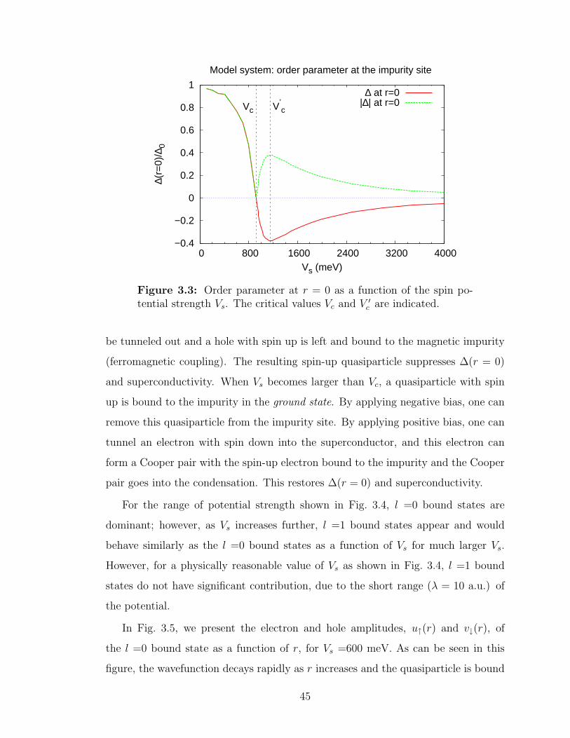
−0.4

−0.2

0

0.2

0.4

0.6

0.8

1

0 800 1600 2400 3200 4000

∆(r=

0)/∆

0

Vs (meV)

Model system: order parameter at the impurity site

Vc V’c

∆ at r=0 |∆| at r=0

Figure 3.3: Order parameter at r = 0 as a function of the spin po-tential strength Vs. The critical values Vc and V ′

c are indicated.

be tunneled out and a hole with spin up is left and bound to the magnetic impurity

(ferromagnetic coupling). The resulting spin-up quasiparticle suppresses ∆(r = 0)

and superconductivity. When Vs becomes larger than Vc, a quasiparticle with spin

up is bound to the impurity in the ground state. By applying negative bias, one can

remove this quasiparticle from the impurity site. By applying positive bias, one can

tunnel an electron with spin down into the superconductor, and this electron can

form a Cooper pair with the spin-up electron bound to the impurity and the Cooper

pair goes into the condensation. This restores ∆(r = 0) and superconductivity.

For the range of potential strength shown in Fig. 3.4, l =0 bound states are

dominant; however, as Vs increases further, l =1 bound states appear and would

behave similarly as the l =0 bound states as a function of Vs for much larger Vs.

However, for a physically reasonable value of Vs as shown in Fig. 3.4, l =1 bound

states do not have significant contribution, due to the short range (λ = 10 a.u.) of

the potential.

In Fig. 3.5, we present the electron and hole amplitudes, u↑(r) and v↓(r), of

the l =0 bound state as a function of r, for Vs =600 meV. As can be seen in this

figure, the wavefunction decays rapidly as r increases and the quasiparticle is bound

45

−1

−0.5

0

0.5

1

1.5

0 800 1600 2400 3200 4000

Eb

/ ∆0

Vs (meV)

Energy of bound states with angular momentum l=0,1

Vcl=0l=0l=1l=1

Figure 3.4: Energies of the bound states with the angular momentuml = 0, 1 as a function of the spin potential strength.

within the region where the order parameter is suppressed (see Fig. 3.2). There is

always a phase shift between the electron and hole components of a bound state.

Figure 3.6 shows the electron and hole amplitudes for a scattering state for l =0 and

Vs = 600 meV. The scattering states extend outside “the potential well” and there

is a phase shift between the two components only very close to the impurity site,

which disappears quickly as r increases.

In Fig. 3.7, the phase shift between the electron and hole components of a spin-up

bound state is plotted as a function of Vs. It can be seen that the phase shift increases

as Vs increases and approaches π in the limit that Vs is very large. The phase shift is

about π/2 at the critical value Vc where the sign of ∆(r = 0) changes from positive

to negative and the energies of the spin-up and spin-down bound states are both

zero. As a result of the phase shift between the electron and hole amplitudes, there

is asymmetry between positive and negative energies in the LDOS (dI/dV ). This is

illustrated in Fig. 3.8, where the tunneling conductance at the impurity site (r = 1

a.u.) is plotted as a function of bias voltage for Vs =600, 916 and 1200 meV. When

Vs < Vc (Vs=600 meV), the peak in the tunneling conductance for positive bias

is higher than that for negative bias. This means that the probability amplitude

46

0

0 0.05 0.1 0.15

Wav

efun

ctio

n (a

rb. u

nit)

r/R

Bound state : Vs=600meV, E=0.4125∆0

u(r)v(r)

Figure 3.5: Electron and hole amplitudes of the l = 0 bound state.

of a spin-up quasiparticle excitation (tunneling an electron in with positive bias)

is larger than that of a spin-down quasiparticle excitation (tunneling an electron

out with negative bias). For Vs > Vc (Vs=1200 meV), the asymmetry is opposite.

As discussed above, in this case, a spin-up quasiparticle is bound to the impurity

in ground state and the hole-like excitation is in favor instead. Such asymmetry

in the tunneling conductance has been observed in the experiment of Yazdani et

al.. They found particle-hole asymmetry in the tunneling conductance over the Mn

atom similar to that for Vs =1200 meV in our model. On the other hand, opposite

asymmetry was observed over Gd, as found for Vs =600 meV by our calculation. We

thus propose, within the classical spin model, that the effective interaction strength

between the magnetic impurity and the conduction electrons is different in these two

materials, resulting in different natures of quasiparticle excitations. Changes of the

nature of bound states as Vs varies are illustrated in Fig. 3.10 and Fig. 3.11, where

dI/dV is plotted as a function of energy and the potential strength Vs. As seen in

Fig. 3.10, bound states appear at the gap edge as Vs increases from zero. Then the

magnitude of the bound state energies decreases as Vs increases, and at Vs = Vc, the

two bound state peaks merge at zero energy. As Vs is increased further (Fig. 3.11),

the zero-bias peak splits and the bound state peaks approach the gap edge. It can

47

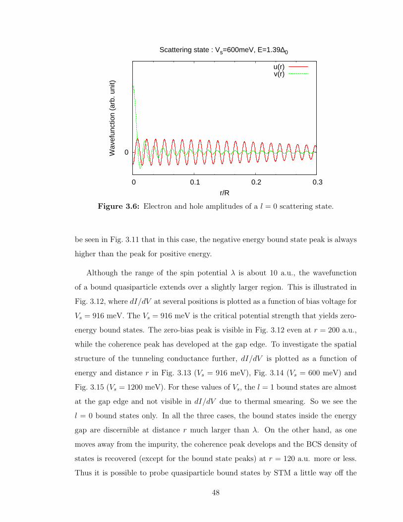
0

0 0.1 0.2 0.3

Wav

efun

ctio

n (a

rb. u

nit)

r/R

Scattering state : Vs=600meV, E=1.39∆0

u(r)v(r)

Figure 3.6: Electron and hole amplitudes of a l = 0 scattering state.

be seen in Fig. 3.11 that in this case, the negative energy bound state peak is always

higher than the peak for positive energy.

Although the range of the spin potential λ is about 10 a.u., the wavefunction

of a bound quasiparticle extends over a slightly larger region. This is illustrated in

Fig. 3.12, where dI/dV at several positions is plotted as a function of bias voltage for

Vs = 916 meV. The Vs = 916 meV is the critical potential strength that yields zero-

energy bound states. The zero-bias peak is visible in Fig. 3.12 even at r = 200 a.u.,

while the coherence peak has developed at the gap edge. To investigate the spatial

structure of the tunneling conductance further, dI/dV is plotted as a function of

energy and distance r in Fig. 3.13 (Vs = 916 meV), Fig. 3.14 (Vs = 600 meV) and

Fig. 3.15 (Vs = 1200 meV). For these values of Vs, the l = 1 bound states are almost

at the gap edge and not visible in dI/dV due to thermal smearing. So we see the

l = 0 bound states only. In all the three cases, the bound states inside the energy

gap are discernible at distance r much larger than λ. On the other hand, as one

moves away from the impurity, the coherence peak develops and the BCS density of

states is recovered (except for the bound state peaks) at r = 120 a.u. more or less.

Thus it is possible to probe quasiparticle bound states by STM a little way off the

48

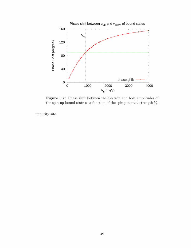
0

40

80

120

160

0 1000 2000 3000 4000

Pha

se S

hift

(deg

ree)

Vs (meV)

Phase shift between uup and vdown of bound states

Vc

phase shift

Figure 3.7: Phase shift between the electron and hole amplitudes ofthe spin-up bound state as a function of the spin potential strength Vs.

impurity site.

49

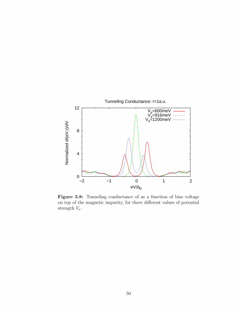
0

4

8

12

−2 −1 0 1 2

Nor

mal

ized

dI(

eV,r

)/dV

eV/∆0

Tunneling Conductance: r=1a.u.

Vs=600meVVs=916meV

Vs=1200meV

Figure 3.8: Tunneling conductance of as a function of bias voltageon top of the magnetic impurity, for three different values of potentialstrength Vs.

50

Figure 3.9: Difference spectra measured near isolated (A) Mn, (B)Gd, and (C) Ag atom [20].

51

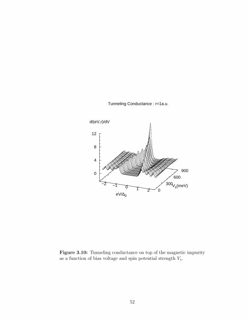
Tunneling Conductance : r=1a.u.

−2 −1 0 1 2eV/∆0

0

300

600

900

Vs(meV)

0

4

8

12

dI(eV,r)/dV

Figure 3.10: Tunneling conductance on top of the magnetic impurityas a function of bias voltage and spin potential strength Vs.

52

Tunneling Conductance : r=1a.u.

−2−1 0 1 2

eV/∆0

900

2400

3900

Vs(meV)

0

4

8

12

dI(eV,r)/dV

Figure 3.11: Same as Fig. 3.10 but for larger Vs.

53

0

4

8

12

−3 −2 −1 0 1 2 3

Nor

mal

ized

dI(

eV,r

)/dV

eV/∆0

Tunneling Conductance: Vs=916meV

r=1a.u.r=20a.u.r=40a.u.

r=200a.u.

Figure 3.12: Tunneling conductance as a function of energy eV atdifferent radial distances r.

54

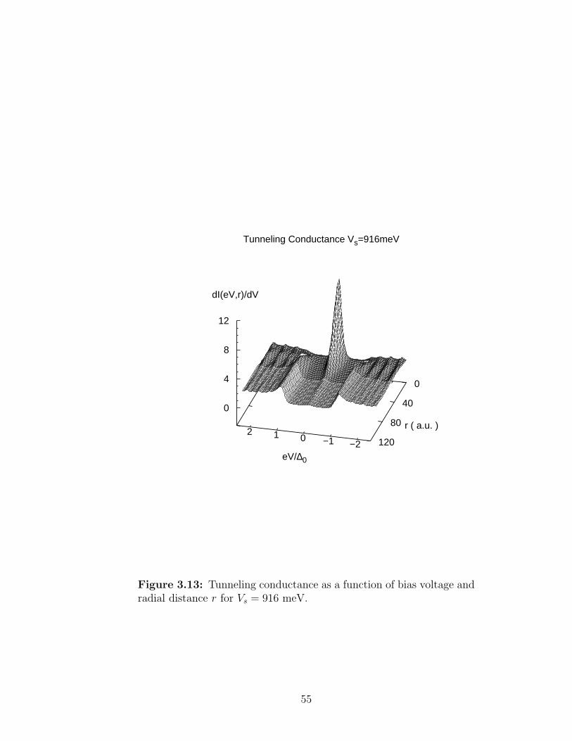
Tunneling Conductance Vs=916meV

−2−1 0 1 2

eV/∆0

0

40

80

120

r ( a.u. )

0

4

8

12

dI(eV,r)/dV

Figure 3.13: Tunneling conductance as a function of bias voltage andradial distance r for Vs = 916 meV.

55

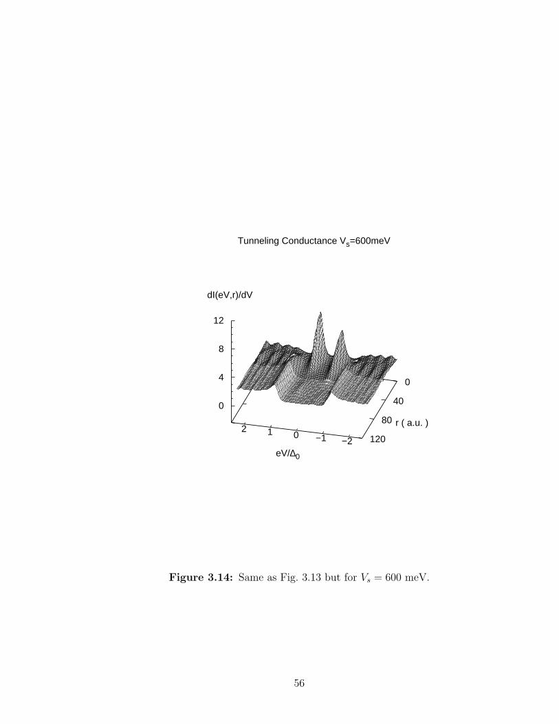
Tunneling Conductance Vs=600meV

−2−1 0 1 2

eV/∆0

0

40

80

120

r ( a.u. )

0

4

8

12

dI(eV,r)/dV

Figure 3.14: Same as Fig. 3.13 but for Vs = 600 meV.

56

Tunneling Conductance Vs=1200meV

−2−1 0 1 2

eV/∆0

0

40

80

120

r ( a.u. )

0

4

8

12

dI(eV,r)/dV

Figure 3.15: Same as Fig. 3.13 but for Vs = 1200 meV.

57

Chapter 4

Conclusion

4.1 Conclusion

In this thesis, to study inhomogeneous superconductivity around a single magnetic

impurity, we have used the BdG theory of superconductivity including a magnetic

interaction, and have developed program for solving the BdG equations selfconsis-

tently, utilizing parallel computation. We have examined in detail the order pa-

rameter, quasiparticle excitation spectra, quasiparticle wavefunctions, and the local

tunneling conductance.

In order to check the accuracy of the computational programming of the BdG

equations, we have first studied the problem of a single magnetic vortex and solved

the BdG equations for a two-dimensional superconductor, NbSe2. The tunneling

conductance around a vortex exhibits Andreev bound states of quasiparticles trapped

in the “potential well” of the order parameter. This result is consistent with both

experimental [11] and earlier theoretical [26] works.

We have then generalized our BdG equations to three-dimensional systems, and

after reproducing the well-known BCS results for a homogeneous superconductor,

we have investigated the effects of a single magnetic impurity by modeling the im-

purity by a classical spin and solving the spin-dependent BdG equations. The BdG

equations were solved directly and numerically, until selfconsistency for the order

parameter was obtained. Unlike the conventional BCS theory, which assumes trans-

lational invariance, selfconsistently solving the BdG equations has high numerical

demand. Our study of inhomogeneous superconductivity has been made feasible by

means of parallel computation on a large-scale Beowulf-class PC cluster here at the

58

University of Saskatchewan. Modeling Nb, the experimentally studied superconduc-

tor [20], is still not practical due to its very large Fermi energy, so we have performed

our calculation for a model system similar to NbSe2.

Similar to a vortex, a magnetic impurity tends to break up Cooper pairs and

suppress superconductivity locally, trapping quasiparticles around it. A significant

difference, however, from the vortex problem is that the magnetic impurity aligns the

spin of the neighboring conduction electrons with its own. This results in particle-

hole asymmetry in the local density of states and the tunneling conductance.

As the effective potential from the magnetic impurity has a very short range on

the atomic scale, bound states exist for angular momentum l = 0 and 1 only, for a

physically reasonable potential strength. We find two bound-state branches (l = 0),

one for a spin-up quasiparticle (spin-up electron and spin-down hole) and another for

a spin-down quasiparticle (spin-down electron and a spin-up hole). As the potential

strength V increases from zero, the two bound states appear near the gap edge –

with positive energy for spin-up quasiparticle and negative energy for spin-down

quasiparticle – and as a function of V , their bound-state energies approach zero and

cross at zero energy at a certain critical strength Vc . Beyond this critical strength,

the two bound-state energies reverse their sign, and the nature of the quasiparticle

bound states changes from that for V < Vc.

For V < Vc, the positive-energy bound state represents adding a quasiparticle

excitation with spin up, and the negative-energy state corresponds to removing a

quasiparticle with spin down. For V > Vc, however, the magnetic interaction with the

impurity is so strong that, in the ground state, there is already a spin-up quasiparticle

bound to the impurity. Thus the negative-energy excitation is the removal of this

quasiparticle. On the other hand, the positive-energy state corresponds to adding

a spin-down quasiparticle (spin-down electron or spin-up hole), which will form a

Cooper pair with the bound spin-up quasiparticle and enter into the superconductor.

Our results for the tunneling conductance with particle-hole asymmetry are con-

sistent with what has been observed experimentally [20]. In the experiment of

Ref. [20], the tunneling conductance over a Mn atom and that over a Gd atom

59

showed opposite asymmetry. We propose that, within our model of a classical spin,

this difference comes from a difference in the effective interaction between the mag-

netic atom and the conduction electrons in the case of Mn (V > Vc) and Gd (V < Vc).

60

References

[1] H. Kamerlingh Onnes. Communications from Physics Laboratory at the Uni-versity of Leiden, page 119, 1911.

[2] W. Meissner and R. Ochsenfeld. Naturwissenschaften, 21:787, 1933.

[3] J. Bardeen, L. Cooper, and R. Schrieffer. Physical Review, 106:162, 1957.

[4] J. Bardeen, L. Cooper, and R. Schrieffer. Physical Review, 108:1175, 1957.

[5] J. Bardeen and R. Schrieffer. Progress in Low Temperature Physics, 3:170, 1961.

[6] J. Gavala. Applied Physics Letters, 23:480, 1978.

[7] J. Bednorz and K. Muller. Zeitschrift fur Physik B, 64:189, 1986.

[8] A. Abrikosov. Soviet Physics-Journal of Experimental and Theoretical Physics,5:1175, 1957.

[9] P. de Gennes. Superconductivity of Metals and Alloys. Boulder, CO: WestviewPress, 1999.

[10] U. Essmann and H. Trauble. Physics letters A, 24:526, 1967.

[11] H. Hess, R. Robinson, R. Dynes, J. Valles, and J. Waszczak. Physical ReviewLetters, 62:214, 1989.

[12] H. Hess, R. Robinson, R. Dynes, J. Valles, and J. Waszczak. Journal of VacuumScience Technology, A 8:450, 1990.

[13] C. Caroli, P. de Gennes, and J. Matricon. Physics Letters, 9:307, 1964.

[14] C. Caroli, P. de Gennes, and J. Matricon. Physics Condense Matter, 3:380,1965.

[15] K. Tanaka, I. Robel, and B. Janko. Proceedings of the National Academy ofSciences of the United States of America, 99:5233, 2002.

[16] P. Anderson. Journal of Physics and Chemistry of Solids, 11:26, 1959.

[17] K. Tanaka and F. Marsiglio. Physical Review B, 62:5345, 2000.

[18] A. Abrikosov and L. Gor’kov. Soviet Physics-Journal of Experimental and The-oretical Physics, 10:593, 1960.

61

[19] A. Abrikosov and L. Gor’kov. Soviet Physics-Journal of Experimental and The-oretical Physics, 12:1243, 1961.

[20] A. Yazdani, B. Jones, C. Lutz, M. Crommie, and D. Eigler. Science, 275:1767,1997.

[21] L. Landau. Soviet Physics-Journal of Experimental and Theoretical Physics,3:920, 1956.

[22] N. Bogoliubov. Nuovo Cimento, 7:794, 1958.

[23] J. Valatin. Nuovo Cimento, 7:843, 1958.

[24] J. Schrieffer. Theory of Superconductivity. CO:Westview Press, 1971.

[25] M. Cyrot and D. Pavuna. Introduction to Superconductivity and High-TC Ma-terials. World Scientific Publishing Co. Pte. Ltd., 1992.

[26] F. Gygi and M. Schluter. Physical Review B, 43:7609, 1991.

[27] M. Tinkham. Introduction to Superconductivity. Doven Publication, Inc., secondedition.

[28] B. Deaver and W. Fairbank. Physical Review Letters, 7:43, 1961.

[29] R. Doll and M. Nabauer. Physical Review Letters, 7:51, 1961.

[30] T. Smith and H. Rorschach. Reviews of Modern Physics, 36:277, 1964.

[31] V. Moshchalkov, L. Gielen, C. Strunk, R. Jonckheere, X. Qiu, C. VanHae-sendonck, and Y. Bruynseraede. Nature, 373:319, 1995.

[32] K. Geim, V. Grigoreva, V. Dubonos, S. Lok, C. Maan, E. Filippov, andM. Peeters. Nature, 390:259, 1997.

[33] Y. Tanaka, A. Hasegawa, and H. Takayanagi. Solid State Communications,85:321, 1993.

[34] M. Virtanen and M. Salomaa. Physical Review B, 60:14581, 1999.

[35] J. Sonier, R. Kiefl, J. Brewer, S. Dunsiger J. Chakhalian, W. MacFarlane,R. Miler, A. Wong, G. Luke, and J. Brill. Physical Review Letters, 79:1742,1997.

[36] J. Fletcher, A. Carrington, P. Diener, P. Rodiere, J. Brison, R. Prozorov, T. Ol-heiser, and R. Giannetta. Physical Review Letters, 98:057003, 2007.

[37] P. Diener, P. Rodiere, J. Fletcher, A. Carrington, J. Brison, R. Prozorov, T. Ol-heiser, and R. Giannetta. Phyica C, 60:460, 2007.

62

[38] A. Andreev. Soviet Physics-Journal of Experimental and Theoretical Physics,19:5, 1964.

[39] L. Kramer and W. Pesch. Zeitschrift fur Physik A Hadrons and Nuclei, 269:59,1974.

[40] A. Unsold. Annalen der Physik, 82:355, 1927.

[41] S. Barnes. Advances in Physics, 30:801, 1981.

[42] J. Schrieffer and P. Wolff. Physical Review, 149:491, 1966.

[43] C. Kessler, M. Mehring, P. Castellaz, G. Borodi, C. Filip, A. Darabont, andL. Giurgiu. Physica B:Condensed Matter, 229:113, 1997.

[44] P. Joseph and P. Singh. Solid State Communications, 141:390, 2007.

[45] K. Baberschke. Zeitschrift fur Physik B, 24:53, 1976.

[46] D. Morr and J. Yoon. Physical Review B, 73:224511, 2006.

[47] W. Press, B. Flannery, S. Teukolsky, and W. Vetterling. Numerical Recipes inC: The Art of Scientific Computing. Cambridge University Press, 2nd edition,1992.

[48] M. Mori and R. Piessens. Numerical Quadrature. Elsevier Science Pub. Co., 1stedition, 1987.

[49] J. Mathews. Numerical Methods for Mathematics, Science, and Engineering.Englewood Cliffs, second edition, 1992.

63

Appendix A

Parallel Computation

Traditionally, a program runs on a single personal computer (PC) with a singleCPU. Instructions are executed sequentially, and only one instruction can be exe-cuted at any moment. But in parallel computing, a program runs on more than oneCPU at the same time. A problem is broken into different parts that are executedconcurrently on different CPUs.

Because of constraints to building a PC with faster CPU and/or larger memory,it is believed that parallelism is the future of computing. Parallel computing ona pc cluster can save time, overcome memory constraints, and save costs by usingmultiple “cheap” PCs instead of a supercomputer. Parallel computation often makesnumerical calculations for complex systems feasible.

A.1 Hardware

Our computation is performed on a Beowulf-class PC cluster, a 128-CPU 3GHZXeon cluster with Hyperthreading Technology, which allows one to use the clusteras having 256 CPUs. The PCs are connected via an extremely fast, low-latencynetwork

There are mainly two kinds of memory architectures of a PC cluster, sharedmemory and distributed memory. The general characteristics of shared memoryare that all processors have access to all memory as global address space (Fig. A.1).Different processors can operate independently but share the same memory resource,and changes in a memory location made by one processor are visible to all otherprocessors. On the contrary, the distributed memory structure is that each processorhas its own local memory (Fig. A.2). Fast interconnection among different CPUsare vital for data transfer on a large-scale cluster. The computer cluster used for ourproject has the distributed memory architecture.

A.2 Software

Message Passing Interface (MPI) is currently the most versatile model of parallelprogramming that is portable and most suitable for the distributed-memory archi-tecture. It can be used even on a shared-memory machine. The MPI has beenapplied for the calculation presented in this thesis. The basic procedure of MPI isthat the “master” process sends out input data to all the “slave” processes by Com-mands such as Send and Receive or Bcast (broadcasting), and each process thendoes its part of the calculation and sends (Send) the result back to the master node(Receive). In this last procedure of data collection, for example, calculation such

64

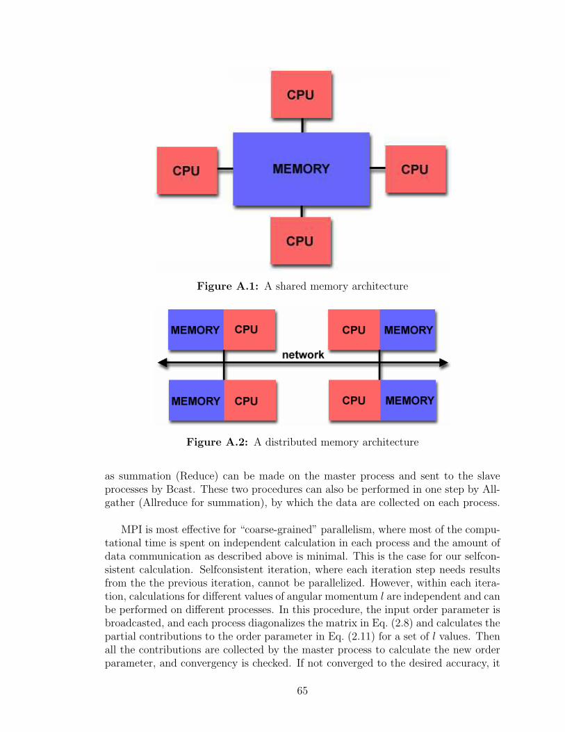
Figure A.1: A shared memory architecture

Figure A.2: A distributed memory architecture

as summation (Reduce) can be made on the master process and sent to the slaveprocesses by Bcast. These two procedures can also be performed in one step by All-gather (Allreduce for summation), by which the data are collected on each process.

MPI is most effective for “coarse-grained” parallelism, where most of the compu-tational time is spent on independent calculation in each process and the amount ofdata communication as described above is minimal. This is the case for our selfcon-sistent calculation. Selfconsistent iteration, where each iteration step needs resultsfrom the the previous iteration, cannot be parallelized. However, within each itera-tion, calculations for different values of angular momentum l are independent and canbe performed on different processes. In this procedure, the input order parameter isbroadcasted, and each process diagonalizes the matrix in Eq. (2.8) and calculates thepartial contributions to the order parameter in Eq. (2.11) for a set of l values. Thenall the contributions are collected by the master process to calculate the new orderparameter, and convergency is checked. If not converged to the desired accuracy, it

65

Figure A.3: Message Passing Interface model

initiates the next iteration. A flow chart of this procedure is shown in Fig. A.4.

The order parameter is calculated at discretized positions {ri; i = 1, ..., N}. Theconvergence is checked by summing the local error, ∆new(ri) − ∆old(ri), over i anddividing the sum by N . We require that the average error is smaller than 10−4.Double precision is used for all the calculations presented in this thesis, and theBessel functions are expected to be accurate to 10−16.

Figure A.4: Flow Chart of the Computation

66

A.3 Computation

A.3.1 Homogeneous System in Two Dimensions

For a homogeneous system in two dimensions, the submatrices T and ∆ are bothdiagonal as shown in Eqs. (2.9, 2.10), and those diagonal elements are easy to ob-tain. This real, symmetric matrix is reduced to a tridiagonal form by Householderreduction [47] and the reduced matrix is solved by QL algorithm [47].

A.3.2 Isolated Vortex Problem

The calculation procedure of the vortex problem is basically the same as that of thehomogeneous model as shown in Fig. A.4. However, the pairing potential is now afunction of position and the submatrix ∆ is no longer diagonal (Eq. (2.28)). Theevaluation of the matrix elements is time-consuming and the calculation is coarse-grained. The integration is difficult due to strong oscillations of the Bessel function,especially when the nodal quantum number is large. Several integration algorithmswere tried, including routines trapzd, qtrap, qsimp, qromb and qgaus from NumericalRecipes in C [47]. The Fortran routine QAG of the integration package QUADPACKfrom Netlib, which can deal well with a strongly oscillating integrand, has turned tobe most reliable [48].

The pairing potential ∆(r) at the end of each iteration is evaluated at a set of dis-crete positions. To calculate the matrix elements for the next iteration, curve fittingis needed to evaluate ∆(r) at any r required by the integration routine. Interpola-tion and extrapolation are common choices of curve fitting. However, QUADPACKrequires the integrand to be a smooth function. To guarantee smoothness, anotherkind of curve fitting, the trigonometric polynomial method, is used to construct asmooth function to best fit the discrete data of ∆(r). This method is discussed indetails in Appendix B.

A.3.3 Homogeneous System in Three Dimensions

The programs are similar to those for solving the homogeneous problem in twodimensions, except that numerically evaluating the spherical Bessel functions is moredifficult than the Bessel functions of integer order near the origin. This had to betaken care of when performing the integrals for the matrix elements.

A.3.4 Isolated Magnetic Impurity Problem

The numerical evaluation of the matrix elements of ∆ is more difficult than thatin the vortex problem. This is due to the fact that integrating the spherical Besselfunctions costs much more time than integrating the Bessel functions of integer order.To reduce the computation time, the matrix elements were evaluated in two regionsseparately. Since the range of the impurity potential (10 a.u.) is so much smaller thanthe system size (R =8000 a.u.), it can be assumed safely that the order parameter

67

is constant in the region [0.3R:R]. Thus we store the values of the integral in thisregion, and perform the integration only in the region [0:0.3R] at each iteration. The

two parts are combined to yield the matrix elements of ∆.

68

Appendix B

Curve Fitting

The trigonometric polynomial method [49] is used to make curve fitting of thediscrete data of the pairing potential. The basic idea of this method is presentedin the first section and its application to our calculation is explained in the secondsection.

B.1 Trigonometric Polynomial Approximation

A trigonometric polynomial of order M can be written as

TM(x) =a0

2+

M∑j=1

(ajcos(jxπ) + bjsin(jxπ)). (B.1)

When the parameters, aj and bj, are chosen properly, the polynomial TM(x) can fita discrete function {f(xk) : xk}.

Assume that f(x) is periodic with period 2π and there are N + 1 points withequally spaced abscissas in the region [−1, 1]:

xk = −1 +2k

N, (B.2)

where k = 0, 1, · · · , N and N is an integer. An approximate function TM(x) (2M +1 ≤ N) is determined by minimizing the quantity

N∑

k=0

(f(xk)− TM(xk))2 . (B.3)

The coefficients aj and bj of the polynomial are

aj =2

N

N∑

k=1

f(xk)cos(jxk) j = 0, 1, · · · ,M,

bj =2

N

N∑

k=1

f(xk)sin(jxk) j = 1, 2, · · · ,M.

(B.4)

B.2 Fitting the Pairing Potential

The order parameter ∆(r) is evaluated at a discrete set of points by solving theBdG equations. For the next iteration, it is needed as a smooth function of r. To

69

apply the trigonometric polynomial approximation, ∆(r) is extended for normalizedcoordinate r from region [0:1] to region [-1:1]. For the vortex problem, as the orderparameter goes to zero linearly as r → 0, it is assumed to be an odd function,∆(−r) = ∆(r). For the impurity problem, it is assumed to be an even function.

The trigonometric polynomial TM is an approximation whose precision dependson the choice of the parameter M . The larger the M , the closer the approximation tothe original function, but the upper limit is set by 2M + 1 ≤ N . In our calculation,N ≈ 3000. After comparing the curve fitting with different orders M , we believe thata reasonable approximation can be obtained for the order parameter for M = 150.

70