Effects of a Magnetic Field on Turbulent Flow in the Mold ...ccc.illinois.edu/s/Reports13/Mold Flow with EMBr/SINGH-R... · Effects of a Magnetic Field on Turbulent Flow in the Mold

Effects of a Magnetic Field on Turbulent Flow in the MoldRegion of a Steel Caster

RAMNIK SINGH, BRIAN G. THOMAS, and SURYA P. VANKA

Electromagnetic braking (EMBr) greatly influences turbulent flow in the continuous castingmold and its transient stability, which affects level fluctuations and inclusion entrainment. Largeeddy simulations are performed to investigate these transient flow phenomena using an accuratenumerical scheme implemented on a graphics processing unit. The important effect of thecurrent flow through the conducting solid steel shell on stabilizing the fluid flow pattern isinvestigated. The computational model is first validated with measurements made in a scaledphysical model with a low melting point liquid metal and is then applied to a full-scale industrialcaster. The overall flow field in the scale model was matched in the real caster by keeping onlythe Stuart number constant. The free surface-level behaviors can be matched by scaling theresults using a similarity criterion based on the ratio of the Froude numbers. The transientbehavior of the mold flow reveals the effects of EMBr on stability of the jet, top surfacevelocities, surface-level profiles, and surface-level fluctuations.

DOI: 10.1007/s11663-013-9877-x� The Minerals, Metals & Materials Society and ASM International 2013

I. INTRODUCTION

CONTINUOUS casting (CC) is the predominantmethod of producing cast steel and is currently used in95 pct of the world’s production.[1] Because of the largequantities of steel produced, even small improvements incasting quality and defect reduction can result insubstantial savings in the unit production cost. Themold region in the CC process contains a complexturbulent flow with large velocities and is responsible forsurface defects, slag entrainment and other steel qualityproblems. The flow at the top surface of the mold canresult in hook formation if the velocities are notsufficiently large. However, if the surface velocities arevery large, turbulence and shear instabilities can entrainslag from the top surface. If the surface level fluctuates,then the defects can be caused intermittently. Tailoringmold flow provides an opportunity to improve the steelquality. Thus, it is very important to choose nozzlegeometries and operating conditions that produce flowpatterns within an operating window that avoids theseproblems.

Operating conditions which control mold flow andrelated problems include: the mold cross section, castingspeed, submergence depth, mold powder, argon gasinjection, and electromagnetic forces. The application ofa magnetic field is an attractive method to control moldflow because it is nonintrusive and can be adjustedduring operation. There are various types of flowcontrol mechanisms using magnetic fields, with a broadclassification based on the use of static magnetic fields

using DC current for the electromagnets, or movingfields using AC current. Detailed description of thevarious types of applied magnetic fields is given inReference 2. It is well known that the movement ofconducting material under the influence of a magneticfield produces a force opposing the motion, and thusshould be self-stabilizing. However, the application of amagnetic field can change the flow pattern in non-obvious ways.[3,4] Understanding how a magnetic fieldaffects the highly turbulent mold flow in CC is both animportant and challenging task.Several previous studies have attempted to under-

stand the flow in the mold region under the influence ofdifferent static magnetic field configurations such aslocal,[5–9] ruler,[3,9] and flow-control (FC) mold[3,10,11]

configuration. Cukierski and Thomas[5] observed thatapplication of local electromagnetic braking (EMBr)weakens the upper recirculation region and decreasesthe top surface velocity. Harada et al.[9] compared theeffects of local and ruler EMBr systems and claimed thatboth configurations increase surface velocities anddampen high velocities below the mold, and thatconfiguring the ruler configuration below the nozzleports has better braking efficiency and also results inbetter surface stability. Li et al.[10] studied the effect ofFC mold and reported that with application of the twomagnets, one at the meniscus and the second below thenozzle, plug-like flow develops below the mold, and thetop surface velocities were so low that the meniscuswould be prone to freezing.As it is difficult to make measurements in real casters,

owing to the high temperatures of the molten steel,physical models with other conducting working fluids,such as mercury,[9] tin,[10] and eutectic alloys such asGaInSn,[12–14] have been used in the past to study theeffect of magnetic fields. Numerical studies of themold flow have been extensively used to understand

RAMNIK SINGH, MS Student, and BRIAN G. THOMAS andSURYA P. VANKA, Professors, are with the Department of Mechan-ical Science and Engineering, University of Illinois at Urbana-Champaign, Urbana IL, 61801. Contact e-mail: [email protected]

Manuscript submitted April 19, 2013.

METALLURGICAL AND MATERIALS TRANSACTIONS B

the CC process.[3,5,7,8,14–20] Most of the studies exploringmold flow used Reynolds-averaged Navier–Stokes(RANS)[3,5,7,8,20,21] or unsteady RANS (URANS)[14,16]

which compute only the mean flow behavior and modelthe effects of turbulence through turbulence models.However, transient behavior and flow stability is moreimportant to mold flow quality,[22], yet has receivedrelatively less attention. Direct numerical simulations(DNS) resolves the instantaneous flow accurately butare computationally infeasible at the Reynolds numbersinvolved in the CC process. On the other hand, largeeddy simulations (LES) only model the small scales ofturbulence. LES of the mold flow region in CC, withoutEMBr[16,23] and with EMBr,[3,17–19] have been per-formed by a few researchers and were seen to providea better understanding of the transients involved in theprocess.

The instantaneous and the mean behaviors of themold flow are also greatly affected by the electricalconductivity of the solidifying shell.[10,13,14] Li et al.[10]

showed that the incorporation of accurate wall conduc-tivity is necessary as it affects the braking efficiency ofthe magnetic field. Timmel et al.[13] performed experi-ments with GaInSn alloy and concluded that withconducting side walls, the mold flow was very stable asopposed to insulated walls with the same magnetic fieldconfiguration. Miao et al.[14] conducted URANS simu-lations of the GaInSn model to study the effects of wallconductivity. However, to our knowledge, there havebeen no previous studies which performed LES tounderstand the effects of magnetic fields and wallconductivity on real caster geometries.

In the current study, we have studied the mold flowpatterns under the influence of applied magnetic fieldsincorporating the influence of a conducting shell. An in-house computational fluid dynamics code, CUFLOW,was used to perform LES of the MHD flow in the moldregion. The CUFLOW code has been previously vali-dated for several canonical flows such as MHD flows inrectangular ducts[24,25] and also for the GaInSn modelwith electrically insulated walls.[3] In addition, in thecurrent study we use an additional Sub-Grid Scale(SGS) model, called the Coherent-Structure Model(CSM) proposed by Kobayashi,[26] which incorporatesthe effect of anisotropy induced by the applied magneticfields on the filtered scales. The SGS models used in thecurrent study are discussed in detail in Section II–A.The code is first validated by comparing with measure-ments taken in scaled GaInSn model with conductingbrass plates on the wide face walls.[13] These results arepresented in Section IV–A and compared with resultsfor the same model by Chaudhary et al.[3] who per-formed computations assuming insulated walls. Thecode is then used to study a full-scale real continuouscaster of steel under the influence of a magnetic field.Results for the full-scale caster, with and without theapplied magnetic field, are presented in Section V. Thetime-averaged and instantaneous flows, Reynolds stres-ses, turbulent kinetic energy (TKE), surface-level pro-files, and surface-level fluctuations are computed tostudy the effects of ruler EMBr on the details of the flowphenomena and similarity criteria for scaleup.

II. GOVERNING EQUATIONS FOR LES OFMHDFLOW

In the current study, we solve the unsteady three-dimensional filtered Navier–Stokes (N–S) equations andthe filtered continuity equation given by Eqs. [1] and [2],respectively. The effects of the flow phenomena toosmall to be captured by the grid spacing, and thusspatially filtered, are incorporated by an eddy viscosityðmsÞ which is modeled by a SGS model.

@ui@tþ @uiuj

@xj¼ � 1

q@p�

@xiþ @

@xjmþ msð Þ @ui

@xjþ @uj@xi

� ��

þ 1

qFi i ¼ 1; 2; 3 ð1Þ

@uj@xj¼ 0 ½2�

where i,j imply tensor notation, and repeated indicesin a term indicate summation, ui are the three velocitycomponents, p� is the pressure modified to include thefiltered normal stresses ðp� ¼ pþ ð1=3ÞqskkÞ, where p isthe static pressure, q is the fluid density, m is thekinematic viscosity, and Fi in Eq. [1] represents the threeLorentz-force components.The molten steel flowing through the magnetic field

generates an electric current ð~JÞ, which flows throughthe entire domain producing the Lorentz force ~F

� �, and

is given by

~J ¼ r ~Eþ~u� ~B0

� �¼ r � ~r/þ~u� ~B0

� �½3�

This equation has been obtained after neglecting theinduced magnetic field which is usually small comparedwith the applied magnetic field.[27] The charge conser-vation condition, r � ~J ¼ 0, is then used to get anequation for the potential /.

r � rr/ð Þ ¼ r � r ~u� ~B0

� �� ½4�

The Lorentz force ð~FÞ is given by

~F ¼ ~J� ~B0 ½5�

Here r is electrical conductivity, ~E is induced electricfield, / is electric potential, and ~B0 is the appliedmagnetic field.This set of coupled MHD equations is solved by a

finite volume method and implemented on a graphicsprocessing unit (GPU) for fast computation. Thenumerical details of solving these equations have beendiscussed in previous studies[3,24,25,28,29] and hence areonly briefly described in Section III–B.

A. Sub-Grid Scale (SGS) Models

The effects of the turbulent flow scales, too small to becaptured by the computational grid, are incorporated bySGS models. With increase in grid refinement, contribu-


tion of the SGS model diminishes such that the modelededdy viscosity eventually tends to zero as the refinementnears the requirements of a DNS. One of the earliest andthe simplest of the SGS models is the Smagorinskymodel,[30] in which the SGS eddy viscosity is calculated as

ms ¼ CsDð Þ2 S�� ½6�

where Cs is the Smagorinsky constant, D is the grid cell

volume, and S�� is the magnitude to the velocity strain

tensor Sij ¼ 12

@ui@xjþ @uj

@xi

� �. In the current study, two

variants of the Smagorinsky SGS models were used, asdescribed in the following sections.

1. Wall-Adapting Local Eddy-viscosity (WALE)ModelThe WALE model[31] calculates the eddy viscosity with

appropriate scaling to insure a near-zero value close to thewalls: ðay3Þ. This is a favorable feature for studiesinvolving confinedflows.The eddyviscosity is calculatedas

ms ¼ L2s

SdijS

dij

� �3=2

SijSij

� �5=2þ SdijS

dij

� �5=4 ½7�

whereSdij ¼ 1

2 g2ij þ g2ji

� �� 1

3dijg2kk; gij ¼ @ui

@xj;Ls ¼ Cw DxDyð

DzÞ1=3; C2w ¼ 10:6 C2

s ; Cs ¼ 0:18;and4x,4y, and4z are

the grid spacings in x, y, and z directions, respectively.

2. Coherent-structure Smagorinsky (CSM) ModelThe CSM SGS model[32] dynamically calculates the

model parameter: ðCÞ and has been shown to accuratelypredict the relaminarization of a turbulent flow subjectedto a strong magnetic field. The CSM model incorporatesthe anisotropic effects of the applied magnetic field andalso damps the eddy viscosity close to the wall bydynamically calculating the model constant. The modelconstant is calculated using a coherent-structure functionðFCSÞ as shown in Eqs. [8] through [11].

C2s ¼ C ¼ CCSM FCSj j3=2Fx ½8�

CCSM ¼1

22; FCS ¼

Q

E; Fx ¼ 1� FCS ½9�

Wij ¼1

2

@uj@xi� @ui@xj

� �½10�

Q ¼ 1

2WijWij � SijSij

� �E ¼ 1

2WijWij þ SijSij

� �½11�

III. COMPUTATIONAL MODEL

A. Computational Domain, Mesh, and BoundaryConditions

Two different flow geometries were investigated in thecurrent study: a scaled low-melting point liquid–metal

(GaInSn) model with a ruler EMBr field, and acorresponding full-scale caster, six-times larger in everydimension. Figure 1 gives the geometric details, withdimensions corresponding to the real caster domain,with the sectioned region representing the solidified steelshell on the walls of the real caster mold. The maximumfield strength of the ruler EMBr is positioned across thenozzle outlet ports, centered 92 mm below the freesurface of the liquid metal in the scale model, and552 mm (= 6 9 92 mm) in the real caster. The varia-tions of the applied magnetic field within the mold forboth the GaInSn model and the real caster are shown inFigure 2. Dimensions, process parameters, and materialproperties for both geometries are provided in Table I.The GaInSn model has been experimentally studied

with no magnetic braking (Case 1),[12] magnetic brakingwith insulated walls (Case 2),[12] and magnetic brakingwith conducting walls (Case 3).[13] Miao et al.[14] mod-eled all the three cases with URANS. Chaudhary et al.[3]

validated CUFLOW with measurements for Case 1 andCase 2, and also studied the flow features in detail. Case3, which has conducting brass-plated wide-faced walls,also was simulated in the current study to validate themodel by comparing the results with measurements, andalso to investigate the effects of wall conductivity.For the real caster domain, simulations with no

EMBr (Case 4) and with EMBr (Case 5) were per-formed. The computational domain for the real casterincluded both the liquid pool, shown in Figure 3, andthe solidifying shell, which was initialized to move in thecasting direction at the casting speed. The shell thicknesss at a given location below the meniscus was calculatedfrom s ¼ k

ffiffitp

, where t is the time taken by the shell totravel the given distance and the constant k was chosento match the steady-state shell profile predicted frombreak-out shell measurements by Iwasaki and Tho-mas.[33] The scaling factor of six over the GaInSn modelwas chosen to have mold dimensions typical of acommercial continuous slab caster. In the absence ofEMBr, previous studies[34] have found that the Froudesimilarity criterion matches the flow patterns betweena real caster and a 1/3rd scaled water model. In aprevious study with EMBr in a scaled mercury model,[9]

Froude number ðFr ¼ U=ffiffiffiffiffiffigLpÞ and Stuart number

ðN ¼ B20Lr=qUÞ similarity criteria were simultaneously

maintained by scaling the casting speed and the mag-netic field strength. Froude number maintains the ratiobetween inertial and gravitational forces, whereas Stuartnumber maintains the ratio between electromagneticand inertial forces. However, in the current study, onlythe Stuart number was matched between the 1/6th scaledGaInSn model and the corresponding real caster,keeping the magnetic field strength constant at therealistic maximum of 0.31 Tesla. Maintaining Froudesimilarity as well would have required a very highcasting speed of 3.3 m/min, and a higher magnetic fieldstrength of 0.44 Tesla. The applicability of this scaleupcriterion was investigated by comparing the results forthe scale model with the real caster with EMBr.The GaInSn and the real caster computational meshes

consist of 7.6 and 8.8 million brick cells, respectively.The nozzle in the physical model was very long


(20 diameters), and hence, the nozzle inlet flow condi-tions had no effect on the flow entering the mold. Thus,in the computational model, the nozzle was truncated atthe level of the liquid surface in the mold and a fullydeveloped turbulent pipe flow velocity profile (Eq. [12])was applied at the inlet, as used in previous studies.[3,16]

Vz rð Þ ¼ Vcenterlinez 1� r

R

� �17 ½12�

where Vz rð Þ is the mean velocity in the castingdirection as a function of r, which is the distance fromthe center of the circular nozzle inlet, and R is the radiusof the nozzle. The top free surface in the mold was afree-slip boundary with zero normal velocity and zeronormal derivatives of tangential velocity. A convectiveboundary condition (Eq. [13]) was applied to all threevelocity components at the two mold outlet ducts on thenarrow faces (NF) in the case of the scaled model[16] andacross the open bottom of the real caster domain

@ui@tþUconvective

@ui@n¼ 0 i ¼ 1; 2; 3 ½13�

where Uconvective is the average normal velocity acrossoutlet plane, and n is the direction normal to the outletplane.All other boundaries were solid walls, and the wall

treatment previously reported by Werner and Wengle[35]

was applied. In the real caster, the boundaries betweenthe shell and fluid regions were initialized with fixeddownward vertical velocity equal to the casting speed,which accounts for mass transfer from the fluid region to

the solidifying shell. Insulated electrical boundary con-

dition @/@n ¼ 0� �

was applied on the outer-most boundary

of the computational domain. The fluid flow equationswere solved only in the fluid domain, and the MHDequations were solved in the entire computa-tional domain, including the brass walls for the GaInSn

Fig. 1—Geometry of the real caster with the rectangle showing the location of the applied ruler EMBr.

Fig. 2—Applied magnetic field in the x, y, and z directions forGaInSn model and real caster.


domain and the shell (shaded) region for the real casterdomain.

B. Numerical Method and Computational Cost

An in-house code, CUFLOW, was used in the currentstudy which solves the coupled N–S and MHD equa-tions (Eqs. [1] through [5]) on a structured Cartesiangrid. This code uses a fractional step method for thepressure–velocity coupling and the Adams–Bashforthtemporal scheme and second-order finite volume meth-od for discretizing the momentum equations. Thepressure Poisson equation (PPE) and the electric Pois-son equation (EPE) (Eq. [4]) are solved using ageometric multigrid solver. The cases without the EMBrfield were started with a zero initial velocity whereas theEMBr cases were started from a developed instanta-neous flow field from a simulation with no magneticfield.For the GaInSn model, the magnetic field was applied

after 10 seconds of simulation time (200,000 time steps)for the conditions of Case 1. The flow field for Case3 was then allowed to develop for 5 seconds beforestarting to collect the time averages. The time-averagedquantities were stabilized for 2 seconds after which theturbulence statistics were collected for 10 seconds. Thissimulation required a total of 10 days of calendarcomputation time. The real caster simulation was alsostarted first with zero initial velocity and no magneticfield (Case 4). The collection of time averages was

Table I. Process Parameters

GaInSn Model Real Caster

Volume flow rate | nozzle bulk inlet velocity 110 mL/s | 1.4 m/s 4.8 L/s | 1.7 m/sCasting speed 1.35 m/min 1.64 m/minMold width 140 mm 840 mmMold thickness 35 mm 210 mmMold length 330 mm 1980 mmComputational domain length 330 mm 3200 mmNozzle port dimensions ðwidth� heightÞ 8 9 18 mm2 48 9 108 mm2

Nozzle bore diameter ðinner j outerÞ 10 mm | 15 mm 60 mm | 90 mmSEN submergence depth (liquid surface to top of port) 72 mm 432 mmThickness of shell on the wide faces 0.5 mm s ðmmÞ ¼ 2:75

ffiffiffiffiffiffiffiffitðsÞ

pThickness of shell on the narrow faces 0 mm s ðmmÞ ¼ 2:75

ffiffiffiffiffiffiffiffitðsÞ

pFluid material GaInSn eutectic alloy Molten steelViscosity 0.34 9 10�6 m2/s 0.86 9 10�6 m2/sFluid density 6360 kg/m3 7000 kg/m3

Conductivity of liquid ðrliquidÞ 3.2 9 106 1/Xm 0.714 9 106 1/XmConductivity of walls ðrwallÞ 15 9 106 1/Xm 0.787 9 106 1/XmConductivity ratio ðCwÞ 0.13 0.13Nozzle port angle 0 deg 0 degGas injection No NoReynolds number (Re, based on nozzle diameter) 41,176 118,604Hartmann number (Ha ¼ BL

ffiffiffiffiffiffiffiffiffiffir=qm

p, based on mold width) 1670 2835

Froude number (Fr ¼ U=ffiffiffiffiffiffigLp

, based on mold width) 1.19 0.59Stuart number (N ¼ B2

0Lr=qU, based on mold width) 4.84 4.84Cases 1. No-EMBr 4. No-EMBr

2. EMBr with insulated walls 5. EMBr with conducting walls3. EMBr with conducting walls

Fig. 3—Isometric view of the computational domain (fluid flowregion) for the real caster.


started after 10 seconds (200,000 time steps) and theturbulence quantities were calculated after the meansstabilized for 5 seconds. The turbulence quantities werethen averaged for another 15 seconds, requiring a totalof 10 days computing time. For the case with EMBr(Case 5), the developed no EMBr flow field was taken asa starting condition, and the flow was allowed tostabilize for 10 seconds physical time before calculatingthe time-averaged quantities. The turbulence quantitieswere then calculated after the time-averaged quantitieswere stabilized for 5 seconds of physical time afterwhich further averaging for 10 seconds was performed.This calculation required a total of 15 days computationtime.

The computations were performed on a NVIDIAC2075 GPU with 1.15-GHz cuda-core frequency and6-GB memory. The solution times for the EMBr caseswere nearly double that of the cases without EMBr,which also require the solution of the EPE. Thecalculations with EMBr produced approximately55,000 time steps per day for the GaInSn model andapproximately 35,000 time steps per day for the realcaster. The computational expenses due to a larger gridsize and double precision accuracy in the real castercases required larger computing time per time step.

IV. RESULTS FOR THE GaInSn SCALEDMODEL

A. Comparison with Experimental Measurements

Measurements of time-varying horizontal velocityVxð Þ in the GaInSn model were collected at 5 Hz usingan array of ten ultrasonic Doppler velocimetry (UDV)sensors.[12,13] The first sensor was placed at z = �40 mmon the midplane of the NF, and the subsequent ones wereplaced at 10-mm intervals below the first. Figure 4(a)shows the contour plot of measured time-averagedhorizontal velocity.[12,13] The plot on the top is for theinsulated wall case, whereas the lower plot is for theconducting wall case. Figure 4(b) shows the contour plotof the same quantity calculated using CUFLOW forboth cases. However, here the vertical resolution wasmatched with the experimental data by using thecalculated values on ten horizontal lines with positionsmatching those of the UDV sensors in the experimentalsetup. Figure 4(b) shows a good qualitative match withthe measurements for both the insulated and conductingwall cases. Figure 4(c) shows the contour plots of thesame calculated quantity for both cases but with a muchhigher data resolution, using all computational gridpoints. In this plot, the entire jet region is visualized by acontinuous region of high velocity unlike the previousplots. The low vertical resolution, used in the measure-ments, results in graphical artifacts such as two isolatedregions of high velocity in each jet. The plots shown inFigure 4(b) help in comparing the calculated results withthe plots obtained from the measurements, which exhibitalmost exactly the same respective flow fields, includingthe two high-velocity regions in each jet. However, thehigher-resolution contour plots of the same data look

considerably different from the low-resolution contourplots.The application of a ruler magnetic field is known to

deflect the jet upward,[3] and a similar behavior is seen inthe simulation with conducting walls. The time-averagedhorizontal velocity shows that the jet angles for bothconducting and insulated cases are nearly the same, butthe conducting wall case shows less spreading of the jet,before it impinges on the NF, compared with theinsulated wall case. Also, for the conducting case, strongrecirculation regions were seen, just above and below thejet (negative velocity implies flow toward the NF). Thiscontrasts with the insulated wall case, in which verystrong recirculating flow is seen only above the jet. Bothflow fields are in contrast to that without EMBr(presented later) where no recirculation is seen in thiszoomed-in portion of the domain.Figure 5 compares the measured and calculated time-

averaged horizontal velocities on three horizontal lines,90, 100, and 110 mm from the free surface (correspond-ing to the 4th, 5th and 6th sensors) for the case withconducting walls. Results computed using both theWALE SGS model and the CSM SGS model are shown.For the current case, both models give results whichclosely match the measurements, but the CSM SGSmodel is expected to perform better for the real casterbecause of the higher Reynolds number and largerfraction of the energy in the filtered scales. Further, thelarge Stuart number, 4.84, induces anisotropy of theturbulence[36] which is better represented by the CSMSGS model. Thus, henceforth, only those results withonly the CSM SGS model are shown. The agreementbetween the measurements and the calculations is verygood except close to the SEN and NF walls, which isprimarily due to limitations in the UDV measurements.Timmel et al.[12,13] report that the UDV measurementsare inaccurate near the SEN and the walls because of thelow vertical spatial resolution and the interaction of theultrasonic transducer beam with solid surfaces.The transient horizontal velocities measured by

the UDV probes were compared with the calculationsat a point in the jet region, P5 ðx ¼ �41 mm;y ¼ 0 mm; z ¼ 0 mmÞ, in Figure 6(b). In order to matchthe conditions of the transient measurements closely, a0.2-second time average was performed on the calculatedsignal to match the response frequency (5 Hz) of themeasuring instrument.[13] The measured and the time-averaged signals match well.

B. Instantaneous Results

The flow pattern for the EMBr case with insulatedwalls (Case 2) was remarkably different from the samecase with conducting walls (Case 3). The transientdifferences are even greater. Figure 6(a) shows thehistory of horizontal velocity for Case 2 at P5, a typicalpoint in the jet, which contrasts greatly with the historyin Figure 6(b) for Case 3 at the same location. Theinsulated wall case has strong low-frequency fluctua-tions which indicate large scale wobbling of the jets. Thisbehavior is not seen in the conducting wall case. Thecontrasting transient behaviors are clearly visualized in


Figure 7, which show contour plots of instantaneousvelocity magnitude at the midplane between wide facesat two instances, separated by 2 seconds, for both cases.Case 2 has both side-to-side and up-and-down wobblingof the jets, which makes the entire mold flow veryunstable; whereas the jet in Case 3 is relatively stable.

Figure 7 also shows the contours of time-averagedvelocity magnitude for both cases (leftmost column).Case 2 has an asymmetric flow pattern even aftercollecting the mean for 28 seconds, whereas the calcu-lations with conducting walls (Case 3) produced asymmetric time-averaged velocity field after averaging

Fig. 4—Contours of time-averaged horizontal velocity for case 2 (top) and case 3 (bottom) for the GaInSn model caster. (a) Measurements; (b)and (c) calculations using CUFLOW.

Fig. 5—Comparison of time-averaged horizontal velocity between measurements and CUFLOW calculations using WALE SGS model and CSMSGS model for the GaInSn model caster with conducting walls (case 3).


for only 12 seconds. This finding of increased flowstability with conducting walls, and the contrast of veryunstable flow with insulated walls,[3] agrees with previ-ous findings using both experiments and URANSmodels.[13,14]

The change in the flow pattern in the presence of theconducting walls can be explained by the behavior of thecurrent paths.[14] In the case with insulated walls (Case2), the current lines may close either through theconducting-liquid metal or the Hartmann layers (presenton walls perpendicular to the magnetic field). TheHartmann layers are extremely thin (~40 lm in Case3[14]) at high Ha number ðdHa � Ha�1Þ, resulting in highresistance, and thus most of the return current closesthrough the liquid metal itself. The enhanced stability ofthe mold flow in case with conducting walls (Case 3) isenabled by the alternative path provided to the currentthrough the conducting walls. Most of the current isgenerated in the jet region and closes locally through theconducting wall, forming short loops where the mag-netic field is strongest. This prevents the current fromwandering through the flow, where it can generatestrong transient forces causing the unstable flow as seenwith insulated walls. Figure 8(a) shows the time-aver-aged current paths in the regions of the mold withmaximum current for Case 3. These current loops arethe most important because they produce the maximumLorentz forces acting on the flowing metal. Most of thecurrent paths can be seen to go up and through the jet,travel to the conducting walls, move down through theconducting walls (where they are colored gray) and thenback to the jet. Figures 8(b) and (c) show contour plotsof time-averaged current density magnitude for Case3 with vectors in the y–z plane at x ¼ �12 mm (slicethrough the jet) and x–y plane at z ¼ �10 mm (slicethrough the SEN ports), respectively. Figure 8(b) showsthat the maximum current density occurs within theconducting walls near to the nozzle bottom, while withinthe fluid, the maximum is associated with the jet, nearwhere high-velocity fluid intersects with the maximumfield strength. Figure 8(c) shows that there is highcurrent density in the conducting walls all across thewidth of the mold at z ¼ �10 mm. More importantly,

the highest current densities in the fluid region are foundinside and just outside the nozzle ports, decreasingtoward the NFs.

C. Time-Averaged Results

1. Nozzle flowFigures 9(a) and (b) show the time-averaged velocity

magnitude and vectors at the nozzle port for the No-EMBr (Case 1) and EMBr (Case 3) cases, respectively. Itcan be seen that the time-averaged velocity magnitudesare symmetric in the jet region near nozzle port exit forboth cases indicating adequate sample size. The jet in thepresence of the EMBr (Case 3) was deflected upwardand was also much thinner compared with the No-EMBr case. There were two strong recirculation regions,above and below the jet, which return the jet fluid closeto the jet exit.The application of magnetic fields is known to

suppress turbulent fluctuations.[27] This effect is shownin Figure 11 where the w0w0 component of resolvedReynolds stresses is plotted inside the nozzle in themidplane parallel to the NFs. The No-EMBr case hasthe larger fluctuation levels and hence sustains swirl inthe z–y plane which was evident from the high values ofthe w0w0 and v0v0 (not shown) components. The EMBrconfiguration applies a high strength of magnetic field inthe nozzle region which almost completely suppressesthe swirl. The suppression was, however, found to belesser in the conducting wall case. Thus, anothercontributing factor to the stability of the mold flowpattern for the conducting wall case was the bettermixing present in the nozzle, as swirling jet flow isknown to improve jet stability.

2. Mold flowFigure 10(a) shows the contours of time-averaged

velocity magnitude and vectors in the mold for the No-EMBr case. Figure 10(b) also shows the contours oftime-averaged velocity magnitude for the EMBr casewith conducting walls but with streamlines instead ofvectors. Due to the recirculating regions and highgradients close to the jets the vectors masked most of

Fig. 6—Transient horizontal velocity in the jet comparing CUFLOW predictions and measurements in the GaInSn model (a) EMBr with insu-lated walls[3] and (b) EMBr with conducting walls.


the details. The time-averaged velocity magnitude con-tours for both cases were symmetric about the nozzle inthe entire mold region. Also both cases were found tohave stable flow pattern but the No-EMBr (Case 1) casehad a weak upper recirculation region. In Case 3, therecirculation regions were very close to the jet and afterthey reach the nozzle the upper recirculation continuesupward close to the SEN walls whereas the lowerrecirculation continues in the casting direction. Intraditional double-roll flow pattern, which was seen inthe No-EMBr case, the lower recirculation regionextends deep into the mold before returning to the jetregion, whereas in the conducting wall case it is

restricted close to jet with the flow below this regionaligned to the casting direction.The w0w0 component of resolved Reynolds stresses in

the mold region is presented in Figure 11. The resolvedReynolds stresses components, w0w0, v0v0 and u0u0, wererestricted to the jet region in the conducting wall case(Case 3), unlike the insulated wall case (Case 2) wherethe fluctuations extend into the upper mold regionconfirming an unstable flow pattern. This enhancedsuppression in the mold region for the conducting wallcase is attributed to the concentration of the highcurrent density and Lorentz force to the region of

Fig. 7—Time-averaged and instantaneous velocity magnitude (a) EMBr with insulated walls[3] and (b) EMBr with conducting walls (**time afterswitching on EMBr) (all axes in meters).


strongest magnetic field. The resulting stable upper rollflow is beneficial for defect reduction.

3. Surface flowFlow across the top surface is of critical importance to

steel quality. Various defects form if the surface flow iseither too fast or too slow. Figure 12 shows thevariation of time-averaged horizontal surface velocity1 mm below the free surface across the mold width, forCases 1, 2, and 3. In general, the surface velocity in thisGaInSn model is low because of the deep submergencedepth. The No-EMBr case has the lowest surfacevelocity (max = 0.045 m/s) and might be susceptibleto meniscus freezing.[3] The EMBr with conducting wallcase (Case 3) has the highest surface velocities, and the

time-averaged field is also symmetric on both sides. Themaximum time-averaged surface velocity for the EMBrwith insulated wall case (Case 2) lies between that ofCases 1 and 3, and variation across the mold width forthis case was asymmetric about the SEN.The EMBr flow with conducting walls also has the

beneficial effect of lowering the TKE at the surface, asshown in Figure 13. The extremely high and asymmet-ric TKE at the surface for the insulated wall casesuggests large-scale level fluctuations and associatedquality problems. Thus, the effect of the shell conduc-tivity should be considered to accurately study themold flow under the influence of applied magneticfields, especially when considering transient phenom-ena.

Fig. 8—(a) Current paths in the mold close to the nozzle ports. Contour plots of time-averaged current density magnitude on (b) vertical y–zplane at x = �12 mm with vectors of Jy and Jz. (c) Horizontal x–y plane at z = �10 mm with vectors of Jx and Jy.


V. RESULTS FOR THE REAL CASTER

A. Transient Results

1. Effect of EMBr on transient flowHaving validated the CUFLOW model, it was applied

to simulate transient flow in a realistic full-scale com-mercial caster. For both the No-EMBr (Case 4) and theEMBr (Case 5) cases, Figure 14 shows instantaneouscontours of velocity magnitude at two different times, atintervals of one second. It can be seen that with noEMBr, the transient flow field is dominated by small-scale fluctuations. The application of EMBr damps most

of the small-scale fluctuations and deflects the jetsupward. These deflected jets were reasonably stable andthe long time fluctuations were comparable with the No-EMBr case. The flow below the jet region quickly alignsto the casting direction, and the lower roll was restrictedto a small, elongated recirculation loop just below thejet.It has been previously seen that an applied magnetic

field preferentially damps the transient flow fluctuationsparallel to its direction.[27] Figure 15 shows the com-puted time history of two fluctuating velocity compo-nents (y in the thickness direction and z in the casting

Fig. 9—Time-averaged velocity magnitude contours and vectors near nozzle bottom in different cases (66 pct of vectors are skipped for clarity).

Fig. 10—Contours of time-averaged velocity magnitude and vectors/streamlines at mold midplane for (a) no-EMBr case[3] and (b) EMBr casewith conducting walls (83 pct of vectors are skipped for clarity).


direction) at two points P1 (center of SEN bottom) andP2 (near port exit) as previously indicated in Figure 1for the two cases, with and without the magnetic field.The high variation in V0z and V0y at P1 with no EMBrindicates the presence of swirling flow in the nozzlebottom. The frequency of the alternating direction ofthe swirl can be approximated, from the time history ofV0y in Figure 15(a), to be about 1.5 Hz. With EMBr, thelow velocity fluctuations at P1 indicate very little swirl inthe nozzle which results in a smoother jet with less high-frequency turbulent fluctuations. The time history atP2 shows highly anisotropic suppression of turbulence,as the thickness-direction V0y component is dampedmore by the magnetic field.

2. Free surface fluctuations and effect of scalingThe profile of the steel surface level Zsurð Þ and its

fluctuations are of critical importance to the steel qualityas mold slag entrainment and surface defects can occurif the fluctuations are too strong. The surface levelcan be approximated using the pressure method inEq. [14][34] which gives an estimate of the liquid surfacevariation using a potential energy balance.

Zsur ¼p� pmean

qsteelg½14�

The average pressure (pmean) in the current study wascalculated on the horizontal line along the top surface

Fig. 11—w0w0 component of resolved Reynolds stresses at mold mid-planes between wide faces (below) and between narrows faces inside nozzle(above). (a) No-EMBr,[3] (b) EMBr with insulated walls[3] and (c) EMBr with conducting walls (all axes in meters).

Fig. 12—Time-averaged horizontal velocity at the surface plotted against distance from left narrow face.


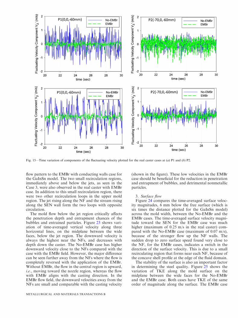
on midplane between the wide faces with g taken as9.81 m/s2. Figure 16 shows three typical instantaneoussurface-level profiles, with a 0.5 seconds moving timeaverage, at three instances separated by 5 seconds each.With no EMBr, the surface level remains almosthorizontal with higher levels (~0.5 mm) close to theNF and SEN. The level variation in the EMBr case wasgreater, because of the increase in momentum, bothclose to the NF (~2.7 mm) and to the SEN (~1.7 mm).The time variation of the level is plotted, at P3 and P4,and is shown is Figure 17. Point P3 is at the midpointbetween the NF and the SEN; and P4 is close to the NFas indicated in Figure 1. The No-EMBr case at bothlocations is found to be stable with only small scalefluctuations. The EMBr case at P3 has small fluctua-tions with oscillation amplitude of ~0.5 mm; whereas atP4 there was a periodic oscillation with amplitude of3 mm and frequency of ~0.2 Hz.

In order to compare the level fluctuations predictedby the GaInSn model with the real caster, they must bescaled. The obvious scaling method is to multiply thescale-model level fluctuations by the geometric lengthscaling factor (=6). However, a better scaling method isto calculate the ratio of the Froude numbers in the twocasters, and rearrange to give the following lengthscaling factor.

LR

LS¼ FrS

FrR

VR

VS

� �2

¼ 2:974 ½15�

where L is the characteristic length scale, V thecharacteristic velocity and the subscripts ‘‘S’’ and ‘‘R’’represent the GaInSn scaled model and the real caster,respectively. Figure 17 compares the scaled level fluctu-ations using both scaling methods, with the real casterhistory, for Case 3 at points P3 and P4. The geometricscaling method overpredicts the average surface-levelposition and its fluctuations in the real caster (Case 5) atboth locations. However, the Froude-number basedscaling factor matches the calculated level fluctuationsin the real caster very closely. This indicates thatthe surface-level fluctuations in scaled models can

accurately predict behavior in the real caster, if theyare scaled based on the Froude-number relationship inEq. [15].

B. Time-Averaged Results

1. Nozzle flowFigure 18 shows the contours of time-averaged veloc-

ity magnitude along with velocity vectors, for the No-EMBr and the EMBr cases. As expected, both contourplots are symmetric about the nozzle centerline indicat-ing adequate time averaging. The jets in the No-EMBrcase exit with a steeper angle (30 deg down) and spreadmore compared with the jets in the EMBr case (10 degdown). Figure 19 shows the variation of time-averagedvelocity magnitude at the vertical line of the midplane ofthe nozzle port exits. The No-EMBr case has a lowertime-averaged velocity magnitude at the top of thenozzle port exit and the value steadily rises around30 mm from the top. The EMBr case also has a lowtime-averaged velocity magnitude at the top of thenozzle port exit but the value remains low more thanhalfway (~60 mm) down the port height. The magnitudethen steadily rises reaching approximately the samemaximum value as the No-EMBr case. This indicatesthat there are flatter (in the Z-direction) and thicker (inthe Y-direction) jets exiting the nozzle ports in thepresence of the EMBr field.The suppression of turbulence in the nozzle by the

magnetic field is shown in Figure 20, where the TKE isplotted with distance down the nozzle port. Thevariation is symmetric for both cases, but the maximumvalue with EMBr is lower by a factor of approximatelyfive. The current EMBr position applies the maximummagnetic field strength directly across the nozzle ports,which causes high suppression of both the turbulentfluctuations and the swirl in the SEN well (Figure 15).The contours of TKE inside the nozzle in the y–zmidplane also aid in visualizing the suppression ofalternating swirl in the nozzle as shown in Figure 21.The No-EMBr case has high TKE values inside thenozzle which were considerably reduced in the presence

Fig. 13—Resolved turbulent kinetic energy at the surface plotted against distance from left narrow face.


of the magnetic field as expected. The vectors of time-averaged velocity field in Figure 21 show the structureof the swirling flow at the nozzle bottom. In the No-EMBr case, the swirls at the SEN bottom are bigger andalso have stronger velocities compared with the EMBrcase. Furthermore, another important effect of theEMBr field on the nozzle flow is seen in the time-averaged velocity profile in the Y-direction (Figure 21)which becomes considerably flat in the presence of theEMBr field. The diagonal components of the Reynoldsstress tensors are not shown for Cases 4 and 5 to avoidredundancy as they were qualitatively similar to theCases 1 and 3 (Figure 11) of the GaInSn model.

2. Mold flowFigure 22 shows the contours of time-averaged veloc-

ity magnitude in the mold region with streamlines forthe No-EMBr and EMBr cases. Time averaging over along time shows the double roll flow pattern presentwith a weaker upper roll. The mean mold flow patternfor the EMBr case is expected to be the same as theGaInSn model EMBr case with conducting wallsbecause Stuart number similarity was used to scale theprocess parameters. Application of the EMBr deflectsthe jets upward resulting in an increased impingingvelocity at higher positions on the NFs. The deflectedjets strengthen the upper roll and create a similar stable

Fig. 14—Instantaneous velocity magnitude for the real caster cases. (a) No-EMBr and (b) with EMBr (*time from start of simulation, **timeafter switching on EMBr).


flow pattern to the EMBr with conducting walls case forthe GaInSn model. The two small recirculation regions,immediately above and below the jets, as seen in theCase 3, were also observed in the real caster with EMBrcase. In addition to this small recirculation region, therewere two other recirculation loops in the upper moldregion. The jet rising along the NF and the stream risingalong the SEN wall form the two loops with oppositecirculation.

The mold flow below the jet region critically affectsthe penetration depth and entrapment chances of thebubbles and entrained particles. Figure 23 shows vari-ation of time-averaged vertical velocity along threehorizontal lines, on the midplane between the widefaces, below the jet region. The downward velocity isalways the highest near the NFs, and decreases withdepth down the caster. The No-EMBr case has higherdownward velocity close to the NFs compared with thecase with the EMBr field. However, the major differencecan be seen further away from the NFs where the flow iscompletely reversed with the application of the EMBr.Without EMBr, the flow in the central region is upward,i.e., moving toward the nozzle region, whereas the flowwith EMBr aligns with the casting direction. In theEMBr flow field, the downward velocities away from theNFs are small and comparable with the casting velocity

(shown in the figure). These low velocities in the EMBrcase should be beneficial for the reduction in penetrationand entrapment of bubbles, and detrimental nonmetallicparticles.

3. Surface flowFigure 24 compares the time-averaged surface veloc-

ity magnitudes, 6 mm below the free surface (which issix times the distance plotted for the GaInSn model)across the mold width, between the No-EMBr and theEMBr cases. The time-averaged surface velocity magni-tude toward the SEN for the EMBr case was muchhigher (maximum of 0.25 m/s in the real caster) com-pared with the No-EMBr case (maximum of 0.07 m/s),because of the stronger flow up the NF walls. Thesudden drop to zero surface speed found very close tothe NF, for the EMBr cases, indicates a switch in thedirection of the surface velocity. This is due to a smallrecirculating region that forms near each NF, because ofthe concave shell profile at the edge of the fluid domain.The stability of the surface is also an important factor

in determining the steel quality. Figure 25 shows thevariation of TKE along the mold surface on themidplane between the wide faces for the No-EMBrand the EMBr case. Both cases have TKE of the sameorder of magnitude along the surface. The EMBr case

Fig. 15—Time variation of components of the fluctuating velocity plotted for the real caster cases at (a) P1 and (b) P2.


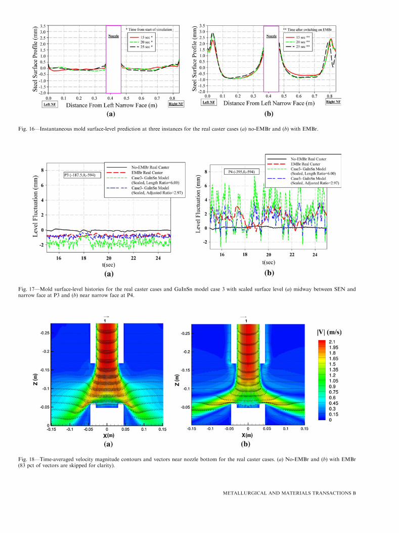
Fig. 16—Instantaneous mold surface-level prediction at three instances for the real caster cases (a) no-EMBr and (b) with EMBr.

Fig. 17—Mold surface-level histories for the real caster cases and GaInSn model case 3 with scaled surface level (a) midway between SEN andnarrow face at P3 and (b) near narrow face at P4.

Fig. 18—Time-averaged velocity magnitude contours and vectors near nozzle bottom for the real caster cases. (a) No-EMBr and (b) with EMBr(83 pct of vectors are skipped for clarity).


has definite peaks of high TKE close to the NF(~0.005 m2/s2) and SEN (~0.002 m2/s2), whereas withno EMBr, the variation along the width was gradual.

4. Effects of scalingThe flow fields predicted for the 1/6 scale-model (Case

3) and the real caster (Case 5) are very similar, eventhough the dimensions differ greatly. The surface-levelprofiles could be matched using appropriate Froude-number based scaling. To further study the validity ofusing Stuart number similarity for scaling EMBr cases,velocities in the GaInSn model were scaled by the ratioof the characteristic velocities in the real caster and theGaInSn model (1.7/1.4 = 1.21, from the inlet velocitiesin Table I). The resulting scaled vertical velocity belowthe jet region is shown in Figure 23(b) along one of thehorizontal lines ðz ¼ 0:40 m; y ¼ 0Þ. The variation ofthe vertical velocities across the width agrees well withthe corresponding real caster curve after shifting andscaling the axes to accommodate for the shell thicknesson the NFs of the real caster. Scaled surface velocitiesare also compared with the calculated values in the realcaster and are seen to agree (Figure 24). The highersurface velocity in the real caster is an effect of thetapered solidifying shell. It has been shown in a previous

study that the tapered shell, and the consequent reduc-tion in cross-section area, deflects more fluid upwardinto the upper recirculation region, leading to theincreased surface velocity.[34]

The agreement between the scaled velocities for Case3 and the velocities for Case 5 is shown more completelyalso in Figure 26. It can be seen that both the flowpatterns as well as the velocity magnitudes match wellover the entire mold.

VI. SUMMARY AND CONCLUSIONS

LES of flow in a full-scale steel caster with the effectsof a ruler magnetic field and conducting steel shell wereperformed. The computational approach was first val-idated with measurements made in a GaInSn physicalmodel[13] and also with simulations with an insulatedelectrical boundary condition. The GaInSn model wasthen scaled to correspond with a full-sized caster andwas studied at conditions similar to industrial opera-tions. However, in order to compare the results with theGaInSn model, the submergence depth was kept pro-portionally the same as the GaInSn model which wasdeeper than typical industrial conditions.

Fig. 19—Time-averaged velocity magnitude plotted along the port midplane vertical line for the real caster cases.

Fig. 20—Resolved turbulent kinetic energy plotted along the port midplane vertical line for the real caster cases.


The large-scale jet wobble and transient asymmetricflow in the mold with insulated walls was not found withconducting walls. With a realistic conducting shell forotherwise identical conditions, the flow was stable, andit quickly achieved a symmetrical flow pattern, whichfeatured three counter-rotating loops in the upper regionand top surface flow toward the SEN. The turbulencedue to Reynolds stresses were suppressed in the presenceof the applied magnetic field. The suppression in theconducting shell case was, however, found to be lower innozzle region. Also, with the conducting shell the

Reynolds stresses were restricted only to the jet regionin the mold. Thus, it is essential to include the effect ofthe conducting shell when studying transient mold flowwith a magnetic field.Relative to the case with no EMBr field, the ruler

magnetic brake across the nozzle deflects the jetsupward, from approximately 30 deg down to only10 deg down. This strengthens the flow in the upperregion and increases the top surface velocity from NF toSEN, from 0.07 to 0.25 m/s in the real caster. Theweaker upper recirculation region without EMBr

Fig. 21—Contours of turbulent kinetic energy with vectors of time-averaged velocity components (Vz and Vy) at mold mid-planes between nar-rows faces inside nozzle for the real caster cases (50 pct of vectors are skipped for clarity).

Fig. 22—Time-averaged velocity magnitude contours and streamlines at mold midplane for the real caster cases. (a) No-EMBr and (b) withEMBr (all axes in meters).


becomes more complex with the application of the rulermagnetic brake, with three distinct recirculation loops,featuring upward flows along both the NF and the SEN.The momentum from these flows raises the surface levelnear the NF and SEN, and generates higher levelfluctuations in these two regions. The lower recircula-tion region becomes a very small elongated loop justbelow the jet, which is similar to a small loop that formsjust above the jet. Flow below this small recirculationloop aligns quickly to the casting direction. These lowerdownward velocities with EMBr should be beneficial forlessening the penetration and entrapment of bubbles andinclusion particles.

The Stuart number similarity criterion employed inthe current study enables a close match of both thetime-averaged mold flow pattern (qualitative) andvelocities (quantitative) between the 1/6-scale modeland the real caster. The scaled surface-level profile andits time fluctuations were matched as well, when usinga scaling factor based on the ratio of the Froudenumbers. Simply scaling the GaInSn model predictionsusing the geometric scale factor of 6 resulted in anoverprediction of the surface-level profile and fluctua-tions, because the Froude number of this scaled modelwas larger than that of the real caster. This Froude-number based scaling method avoids the need to

Fig. 23—Time-averaged vertical velocity (Vz) at three vertical locations in the midplane parallel to the mold wide face plotted against distancefrom narrow face. (a) Real caster no-EMBr case and (b) real caster with EMBr case and GaInSn model EMBr with conducting wall case (scaledvelocity).

Fig. 24—Time-averaged horizontal velocity at the surface plotted against distance from narrow face for the real caster cases and the GaInSnmodel with conducting wall case (scaled velocity).


maintain both Froude number and Stuart numbersimilarity conditions simultaneously when choosingoperating conditions for a scaled model caster withEMBr.

ACKNOWLEDGMENTS

The current study was supported by the NationalScience Foundation Grant CMMI 11-30882 and theContinuous Casting Consortium. The authors are alsograteful to K. Timmel, S. Eckert, and G. Gerbethfrom the MHD Department, ForschungszentrumDresden-Rossendorf (FZD), Dresden, Germany forproviding the velocity measurement database of theGaInSn model experiment with conducting side walls.

REFERENCES1. World Steel in Figures 2012, World Steel Association, Brussels,

Belgium, 2012.2. R. Chaudhary and B.G. Thomas: 6th International Conference on

Electromagnetic Processing of Materials EPM, 2009.3. R. Chaudhary, B.G. Thomas, and S.P. Vanka: Metall. Mater.

Trans. B, 2012, vol. 43B, pp. 532–53.4. C. Zhang, S. Eckert, and G. Gerbeth: J. Fluid Mech., 2012,

vol. 575, pp. 57–82.5. K. Cukierski and B.G. Thomas: Metall. Mater. Trans. B, 2008,

vol. 39B, pp. 94–107.6. D. Kim, W. Kim, and K. Cho: ISIJ Int., 2000, vol. 40, pp. 670–76.7. K. Takatani, K. Nakai, N. Kasai, T. Watanabe, and H. Nakajima:

ISIJ Int., 1989, vol. 29, pp. 1063–68.8. M.Y. Ha, H.G. Lee, and S.H. Seong: J. Mater. Process. Technol.,

2003, vol. 133, pp. 322–39.9. H. Harada, T. Toh, T. Ishii, K. Kaneko, and E. Takeuchi: ISIJ

Int., 2001, vol. 41, pp. 1236–44.10. B. Li, T. Okane, and T. Umeda: Metall. Mater. Trans. B, 2000,

vol. 31B, pp. 1491–1503.

Fig. 25—Resolved turbulent kinetic energy at the surface plotted against distance from the left narrow face for the real caster cases.

Fig. 26—Time-averaged velocity magnitude contour on midplane between wide faces for (a) GaInSn model conducting wall case with scaledvelocity magnitude and (b) real caster with EMBr case (all axes in meters).


11. A. Idogawa, M. Sugizawa, S. Takeuchi, K. Sorimachi, and T.Fujii: Mater. Sci. Eng. A, 1993, vol. 173, pp. 293–97.

12. K. Timmel, X. Miao, S. Eckert, D. Lucas, and G. Gerbeth:Magnetohydrodynamics, 2010, vol. 46, pp. 437–48.

13. K. Timmel, S. Eckert, and G. Gerbeth: Metall. Mater. Trans. B,2011, vol. 42B, pp. 68–80.

14. X. Miao, K. Timmel, D. Lucas, S. Ren, Z. Eckert, and G.Gerbeth: Metall. Mater. Trans. B, 2012, vol. 43B, pp. 954–72.

15. B.G. Thomas and L. Zhang: ISIJ Int., 2001, vol. 41, pp. 1181–93.16. R. Chaudhary, C. Ji, B.G. Thomas, and S.P. Vanka: Metall.

Mater. Trans. B, 2011, vol. 42B, pp. 987–1007.17. Z. Qian, Y. Wu, B. Li, and J. He: ISIJ Int., 2002, vol. 42, pp. 1259–65.18. R. Kageyama and J.W. Evans: ISIJ Int., 2002, vol. 42, pp. 163–70.19. Y. Miki and S. Takeuchi: ISIJ Int., 2003, vol. 43, pp. 1548–55.20. T. Ishii, S.S. Sazhin, and M. Makhlouf: Ironmak. Steelmak., 1996,

vol. 23, pp. 267–72.21. Y. Hwang, P. Cha, H.-S. Nam, K.-H. Moon, and J.-K. Yoon: ISIJ

Int., 1997, vol. 37, pp. 659–67.22. P.H. Dauby: Int. J. Metall., 2012, vol. 109, pp. 113–36.23. Q. Yuan, B.G. Thomas, and S.P. Vanka: Metall. Mater. Trans. B,

2004, vol. 35B, pp. 685–702.24. R. Chaudhary, S.P. Vanka, and B.G. Thomas: Phys. Fluids, 2010,

vol. 22, pp. 075102–15.

25. R. Chaudhary, A.F. Shinn, S.P. Vanka, and B.G. Thomas:Comput. Fluids, 2011, vol. 51, pp. 100–14.

26. H. Kobayashi: Phys. Fluids, 2008, vol. 20, pp. 015102–14.27. R. Moreau: Magnetohydrodynamics, Kluwer, Norwell, MA, 1990,

pp. 110–64.28. A.F. Shinn and S.P. Vanka: J. Turbomach., 2013, vol. 135,

pp. 011004–16.29. A.F. Shinn: Large Eddy Simulations of Turbulent Flows

on Graphics Processing Units: Application to Film-CoolingFlows, University of Illinois at Urbana-Champaign, Urbana,2011.

30. J. Smagorinsky: Annu. Weather Rev., 1963, vol. 96, pp. 99–164.31. F. Nicoud and F. Ducros: Flow Turbul. Combust., 1999, vol. 62,

pp. 183–200.32. H. Kobayashi: Phys. Fluids, 2006, vol. 18, p. 045107.33. J. Iwasaki and B.G. Thomas: Supplemental Proceedings, John

Wiley & Sons, Inc., New York, 2012, pp. 355–62.34. R. Chaudhary, B.T. Rietow, and B.G. Thomas: Mater. Sci.

Technol., AIST/TMS, Pittsburgh, PA, 2009, pp. 1090–1101.35. H. Werner and H. Wengle: 8th Symposium on Turbulent Shear

Flows, 1991, pp. 155–68.36. A. Vorobev, O. Zikanov, P.A. Davidson, and B. Knaepen: Phys.

Fluids, 2005, vol. 17, pp. 125105–16.


Documents

Effects of a Magnetic Field on Turbulent Flow in the Mold ...ccc.illinois.edu/s/Reports13/Mold Flow with EMBr/SINGH-R... · Effects of a Magnetic Field on Turbulent Flow in the Mold