Effects Evaluation of Ambient Vibration Recording Conditions on HVTFA Results S. Atashband Department of Civil engineering, Nowshahr branch, Islamic Azad University, Iran M. Esfahanizadeh Head of Research and Development department, Arzhan Khak Shomal Co., Tehran. Iran.

SUMMARY: Because of ambient vibration benefits in soil seismic properties estimation, several precious researches have been done up to now especially by single station methods. Combining surface wave dispersion curves with the ellipticity of the fundamental mode Rayleigh waves has the advantage of defining the total depth of the soft sediments (Fäh et al., 2008). Recording methods using 3D seismometers have the determinant role in data interpretation process. There are various ways for seismometers installation on ground and there are several restrictions due to some precast structures (e.g. pavements, asphalt or foundations). Signals may be influenced by some of these conditions that lead to discover different results for an individual site in various seismometer installation situations. In this study several installation situations was tested to compare estimated soil properties (e.g. Vs profile based on derived ellipticity curve from H/V spectral ratios analysis (HVTFA)) to evaluate reliability of each seismometer installation method. Keywords: Ambient vibration, 3D seismometer, Vs profile. 1. INTRODUCTION Among several proposed microtremor methods, the H/V technique (e.g. Nakamura, 1989) has proven very convenient for estimating the fundamental frequency of soft deposits (e.g. Tokimatsu, 1997; Bard, 1998; Bonnefoy-Claudet et al., 2006a). This method allows detailed mapping of this frequency within urban areas. In one-dimensional structures, average H/V spectral ratios can also be used to estimate the ellipticity of the fundamental mode Rayleigh wave (e.g. Yamanaka et al., 1994). In the P-SV case, the ellipticity of the ground motion at the free surface is defined as the ratio between the horizontal and vertical displacement eigen-functions at each frequency. Ellipticity is detectable in H/V spectral ratios between the peak at the fundamental frequency of resonance and the first minimum at higher frequency (e.g. Fäh et al., 2001). The shape of the H/V ratio around its maximum peak can thus be used to estimate a shear-wave velocity profile. Yamanaka et al. (1994), Satoh et al. (2001), and Parolai et al. (2006) applied this approach to deep sedimentary basins, while Fäh et al. (2001, 2003) used it for shallow sites (NERIES, 2010). This ellipticity-based method applies only to sites presenting a strong S-wave velocity between sediments and bedrock and when sources are near (4 to 50 times the layer thickness) and close to the surface (Bonnefoy-Claudet et al., 2006b). Most seismic codes adopt the average shear-wave velocity as a key parameter in the first 30 m of subsoil (VS30). Estimates of VS30 are therefore required for both large- and small-scale seismic microzonation. Some techniques have proposed to measure the VS30 based on the horizontal to vertical spectral ratio (H/V) of microtremor recorded at a single station (e.g. Castellaro et al., 2009). By these methods the H/V is fitted with a synthetic curve using the independently known thickness of a superficial layer of the subsoil as a constraint. These proposed procedures consist of three steps: (1) identify the depth of a shallow stratigraphic horizon from independent geotechnical data, (2) identify its corresponding H/V marker, and (3) use it as a constraint to fit the experimental H/V curve with the theoretical one. (Castellaro et al., 2009)

2. PROBLEM EXPLANATION Recent researches indicate recording operation is influenced by several factors including atmospheric and weather conditions, wave's property and source (e.g. natural, human) and system installation conditions. The last one is more controllable. In other words, there are various ways for seismometers installation on a site ground including: direct contact with virgin soil layer (i.e. immediacy) and or using artificial contact (e.g. steel plate, thin sand layer, pavement, etc.). Sometimes, precast area with concrete (e.g. on top of foundation) or asphalt (e.g. on a road) may constrain recording operation. (See Fig. 2.1.)

 

Figure 2.1. Some hardships in seismometer set up operation. Let's review some notes from SESAME (2004):

1) Avoid plates from "soft" materials such as foam rubber, cardboard, etc. 2) On steep slopes that do not allow correct sensor leveling, install the sensor in a sand pile or in

a container filled with sand. 3) On snow or ice, install a metallic or wooden plate or a container filled with sand to avoid

sensor tilting due to local melting. Always there is a concern that above-mentioned conditions may cause undesirable effects on signals and analysis results. So in this study, at first we consider the validity of results (e.g. the derived Vs profile) of records on virgin soil, then we will compare several setting situations with setting of seismometer (i.e. on virgin soil). Also the effects of recording time duration is surveyed. 3. BASIC PRINCIPLE OF HVTFA METHOD In the time-frequency method of H/V computation, the H/V ratio is not computed from the whole spectra for vertical and horizontal components of the ambient noise signal as in the classical spectral ratio method. Instead, the time-frequency representations of the vertical and both horizontal components are computed using CWT (Continuous Wavelet Transform) as defined by Eqn. 3.1 for a real function x(t) with respect to an analyzing wavelet )(tψ . (NORIES, 2010)

dta

bttx

abaxCWT ∫ ⎟

⎠⎞

⎜⎝⎛∞

∞−

−= .*)(

1),}({

ψ (3.1)

Where parameter a is the dilatation (scaling) parameter and b is the translation parameter. If t is a time, then scale a is inversely proportional to frequency and b is a translation in time. Functions )(tψ (a,b) are defined as Eqn. 3.2 and generated by scaling and translating the mother wavelet )(tψ , forming a set of analyzing wavelets, while the width of an analyzing wavelet in the time or spectral domain is proportional to a. Such a set of functions is called a wavelet family, or more simply wavelets. Moreover, in general, the wavelet function )(tψ has to satisfy the admissibility condition (Daubechies, 1992).

)0,,(,1),(

)( ≠ℜ∈⎟⎠⎞

⎜⎝⎛ −

= abaa

btaba

t ψψ (3.2)

Then the wavelet representations of both horizontal components are merged into one (CWT

H) by Eqn.

3.3 as follows:

22EWCWTNSCWTHCWT += (3.3)

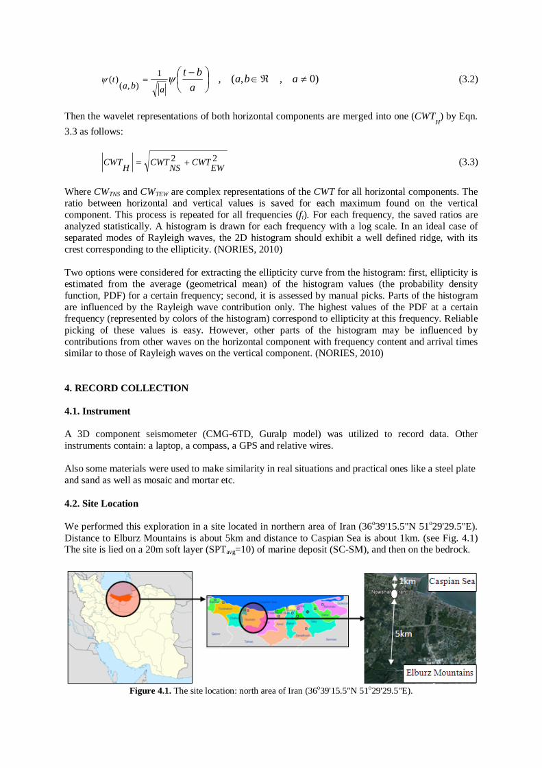
Where CWTNS and CWTEW are complex representations of the CWT for all horizontal components. The ratio between horizontal and vertical values is saved for each maximum found on the vertical component. This process is repeated for all frequencies (fi). For each frequency, the saved ratios are analyzed statistically. A histogram is drawn for each frequency with a log scale. In an ideal case of separated modes of Rayleigh waves, the 2D histogram should exhibit a well defined ridge, with its crest corresponding to the ellipticity. (NORIES, 2010) Two options were considered for extracting the ellipticity curve from the histogram: first, ellipticity is estimated from the average (geometrical mean) of the histogram values (the probability density function, PDF) for a certain frequency; second, it is assessed by manual picks. Parts of the histogram are influenced by the Rayleigh wave contribution only. The highest values of the PDF at a certain frequency (represented by colors of the histogram) correspond to ellipticity at this frequency. Reliable picking of these values is easy. However, other parts of the histogram may be influenced by contributions from other waves on the horizontal component with frequency content and arrival times similar to those of Rayleigh waves on the vertical component. (NORIES, 2010) 4. RECORD COLLECTION 4.1. Instrument A 3D component seismometer (CMG-6TD, Guralp model) was utilized to record data. Other instruments contain: a laptop, a compass, a GPS and relative wires. Also some materials were used to make similarity in real situations and practical ones like a steel plate and sand as well as mosaic and mortar etc. 4.2. Site Location We performed this exploration in a site located in northern area of Iran (36o39'15.5"N 51o29'29.5"E). Distance to Elburz Mountains is about 5km and distance to Caspian Sea is about 1km. (see Fig. 4.1) The site is lied on a 20m soft layer (SPTavg=10) of marine deposit (SC-SM), and then on the bedrock.

Figure 4.1. The site location: north area of Iran (36o39'15.5"N 51o29'29.5"E).

Figure 4.2. Various Situations in signal recording operation: a) Sit1 , b) Sit2 , c) Sit3 , d) Sit4 , e) Sit5 , f) Sit6 (i.e. on the virgin soil)

4.3. Weather Condition The weather was sunny, (hot and humid: approximately, 30oC and 80%) in all recording times. No rain and no strong wind (>5m/s) were observed. 4.4. Situations Description The records have been collected in 6 situations as following: (according to Fig. 4.2) • Sit1: Balcony (Contains: about 2.5cm mosaic + 2cm cement mortar + 50cm basement aggregates

on the virgin soil). • Sit2: Concrete pavement (Contains: about 5cm concrete + 30cm basement aggregates on the

virgin soil). • Sit3: Steel plate & sand (Contains: a steel plate (20 20 1cm) + 3cm marine sand on the virgin

soil). • Sit4: Sand (Contains: 3cm marine sand on the virgin soil). • Sit5: Steel plate (Contains: a steel plate (20 20 1cm) on the virgin soil). • Sit6: Virgin soil (i.e. directly on the virgin soil).

4.5. Recording Time Duration For the situations (1-5) recording time durations were 1 hour. In order to determine a suitable time duration for recording, we decided to compare situation sit6 (i.e. on virgin soil) results by 1 hour duration with one recording in the same situation but a 7-hours record. So as a result, we may evaluate the reliability of 1 hour recording duration and universalize the results to the long ones. 5. ANALYSIS PROCEDURE 5.1. Software Introduction We have used GEOPSY.org package that is a novel programming product in ambient vibration processes (www.GEOPSY.org) including both single and array capabilities as well as a powerful inversion processor (DINVER) that uses neighborhood algorithm which is one of the newest ones. For HVTFA analysis, it presents a user friendly screen and options. Unfortunately, we did not bring the all pretty and comprehensive graphical outputs in this paper (due to the space dearth) but we concluded those output results in some graphs for comparison puporses instead. 5.2. Analysis Steps The analysis has 3 principal steps as follows:

• HVTFA analysis (computation of H/V curves with a time-frequency analysis using wavelet transform as described above, theoretically)

• Ellipticity curve extraction (success in this part is related to interpreter by the geotechnical experiences).

• Inversion process to derive an accurate Vs profile. The program uses the algorithm for an HVTFA analysis as follows (NERIES, 2010): 1- For all three components, the average value is subtracted (DC removal) and the Fourier spectra

are calculated.

2- The modified Morlet wavelet in the frequency domain centered around the frequency fc is given by Eqn. 5.1 as follows:

⎟⎟

⎠

⎞

⎜⎜

⎝

⎛⎟⎟⎠

⎞⎜⎜⎝

⎛−− m

ff

c

2

00exp41 ωωπ

(5.1)

Where, f is the frequency, 0ω is the first Morlet parameter (> 5.5), and m is the second Morlet parameter. This function is convoluted with the three components and then transformed back into the time domain, providing a complex signal there; 0ω is set to 6 and only m is kept as a varying parameter (in this exploration is converged to 10) .

3- The complex signals for horizontal components (North and East) are grouped together with a vectorial combination as Eqn. 5.2.

22 EastNorth + (5.2)

4- The absolute values of the complex vertical and the complex, combined horizontal components

are calculated. 5- For all maxima (including the local) on the vertical component, the time and amplitude are kept.

Amplitudes on the horizontal component are measured at times shifted by +/-90° relative to the vertical peaks.

6- All amplitudes and the ratios of the horizontal over vertical amplitudes are output.

7- The points 2 to 6 are repeated for all frequencies fc chosen by the user.

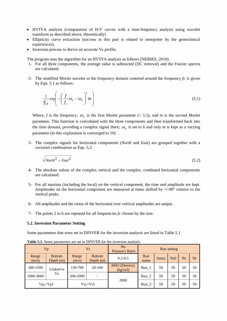
5.2. Inversion Parameter Setting Some parameters that were set in DINVER for the inversion analysis are listed in Table 5.1. Table 5.1. Some parameters are set in DINVER for the inversion analysis.

Vp Vs Nu Poisson's Ratio Run setting

Range (m/s)

Bottom Depth (m)

Range (m/s)

Bottom Depth (m) 0.2-0.5 Run

name Itmax Ns0 Ns Nr

300-1500 Linked to Vs

150-700 20-100 RHO (Density) (kg/m3) Run_1 50 50 50 50

1000-3000 200-2000 - 2000

Run_2 50 50 50 50

Vp0>Vp1 Vs0>Vs1 Run_3 50 50 50 50

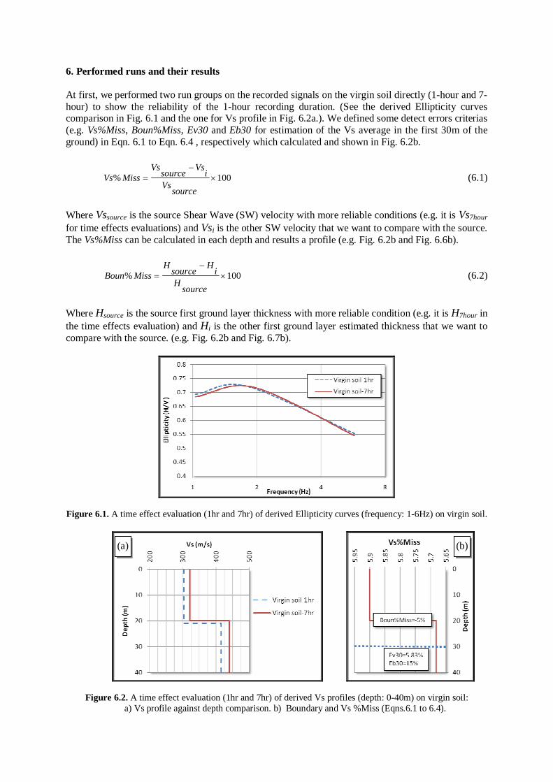
6. Performed runs and their results At first, we performed two run groups on the recorded signals on the virgin soil directly (1-hour and 7-hour) to show the reliability of the 1-hour recording duration. (See the derived Ellipticity curves comparison in Fig. 6.1 and the one for Vs profile in Fig. 6.2a.). We defined some detect errors criterias (e.g. Vs%Miss, Boun%Miss, Ev30 and Eb30 for estimation of the Vs average in the first 30m of the ground) in Eqn. 6.1 to Eqn. 6.4 , respectively which calculated and shown in Fig. 6.2b.

100% ×−

=sourceVs

iVssourceVsMissVs (6.1)

Where Vssource is the source Shear Wave (SW) velocity with more reliable conditions (e.g. it is Vs7hour for time effects evaluations) and Vsi is the other SW velocity that we want to compare with the source. The Vs%Miss can be calculated in each depth and results a profile (e.g. Fig. 6.2b and Fig. 6.6b).

100% ×−

=sourceH

iHsourceHMissBoun (6.2)

Where Hsource is the source first ground layer thickness with more reliable condition (e.g. it is H7hour in the time effects evaluation) and Hi is the other first ground layer estimated thickness that we want to compare with the source. (e.g. Fig. 6.2b and Fig. 6.7b).

Figure 6.1. A time effect evaluation (1hr and 7hr) of derived Ellipticity curves (frequency: 1-6Hz) on virgin soil.

Figure 6.2. A time effect evaluation (1hr and 7hr) of derived Vs profiles (depth: 0-40m) on virgin soil: a) Vs profile against depth comparison. b) Boundary and Vs %Miss (Eqns.6.1 to 6.4).

(a) (b)

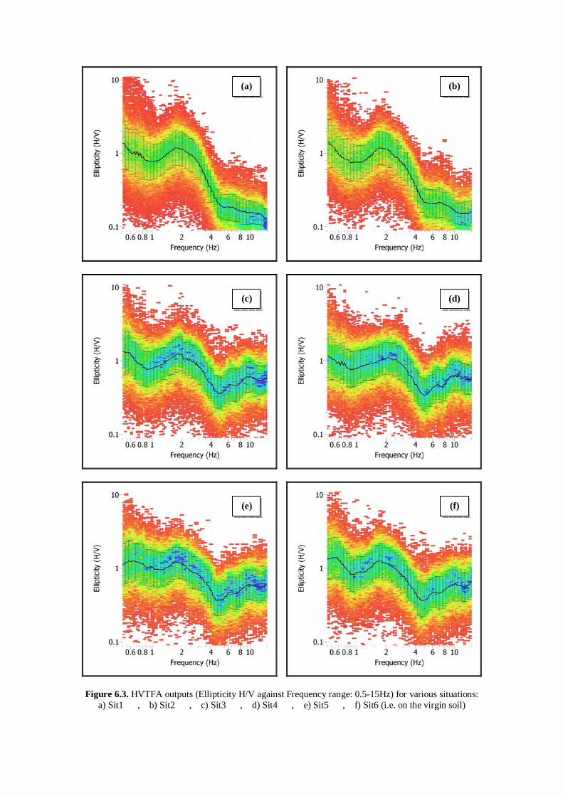
Figure 6.3. HVTFA outputs (Ellipticity H/V against Frequency range: 0.5-15Hz) for various situations: a) Sit1 , b) Sit2 , c) Sit3 , d) Sit4 , e) Sit5 , f) Sit6 (i.e. on the virgin soil)

(a) (b)

(c) (d)

(e) (f)

Figure 6.4. Inversion outputs (Vs profile against Depth range: 0-40 m) for various situations: a) Sit1 , b) Sit2 , c) Sit3 , d) Sit4 , e) Sit5 , f) Sit6 (i.e. on the virgin soil)

(a) (b)

(c) (d)

(e) (f)

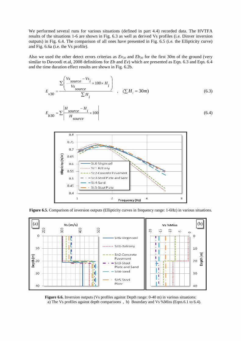
We performed several runs for various situations (defined in part 4.4) recorded data. The HVTFA results of the situations 1-6 are shown in Fig. 6.3 as well as derived Vs profiles (i.e. Dinver inversion outputs) in Fig. 6.4. The comparison of all ones have presented in Fig. 6.5 (i.e. the Ellipticity curve) and Fig. 6.6a (i.e. the Vs profile). Also we used the other detect errors criterias as Ev30 and Eb30 for the first 30m of the ground (very similar to Davoodi et.al, 2008 definitions for Eb and Ev) which are presented as Eqn. 6.3 and Eqn. 6.4 and the time duration effect results are shown in Fig. 6.2b.

)30(,

100

30mHi

iH

iHsourceVs

iVssourceVs

vE =∑

∑

∑ ⎟⎟⎠

⎞⎜⎜⎝

⎛××

−

= (6.3)

∑ ×−

= 10030

sourceHiHsourceH

bE (6.4)

Figure 6.5. Comparison of inversion outputs (Ellipticity curves in frequency range: 1-6Hz) in various situations.

Figure 6.6. Inversion outputs (Vs profiles against Depth range: 0-40 m) in various situations: a) The Vs profiles against depth comparisons , b) Boundary and Vs %Miss (Eqns.6.1 to 6.4).

(a) (b)

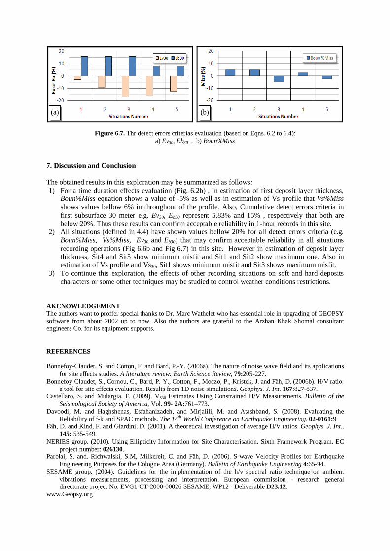
Figure 6.7. Thr detect errors criterias evaluation (based on Eqns. 6.2 to 6.4): a) Ev30, Eb30 , b) Boun%Miss

7. Discussion and Conclusion The obtained results in this exploration may be summarized as follows: 1) For a time duration effects evaluation (Fig. 6.2b) , in estimation of first deposit layer thickness,

Boun%Miss equation shows a value of -5% as well as in estimation of Vs profile that Vs%Miss shows values bellow 6% in throughout of the profile. Also, Cumulative detect errors criteria in first subsurface 30 meter e.g. Ev30, Eb30 represent 5.83% and 15% , respectively that both are below 20%. Thus these results can confirm acceptable reliability in 1-hour records in this site.

2) All situations (defined in 4.4) have shown values bellow 20% for all detect errors criteria (e.g. Boun%Miss, Vs%Miss, Ev30 and Eb30) that may confirm acceptable reliability in all situations recording operations (Fig 6.6b and Fig 6.7) in this site. However in estimation of deposit layer thickness, Sit4 and Sit5 show minimum misfit and Sit1 and Sit2 show maximum one. Also in estimation of Vs profile and Vs30, Sit1 shows minimum misfit and Sit3 shows maximum misfit.

3) To continue this exploration, the effects of other recording situations on soft and hard deposits characters or some other techniques may be studied to control weather conditions restrictions.

AKCNOWLEDGEMENT The authors want to proffer special thanks to Dr. Marc Wathelet who has essential role in upgrading of GEOPSY software from about 2002 up to now. Also the authors are grateful to the Arzhan Khak Shomal consultant engineers Co. for its equipment supports. REFERENCES Bonnefoy-Claudet, S. and Cotton, F. and Bard, P.-Y. (2006a). The nature of noise wave field and its applications

for site effects studies. A literature review: Earth Science Review, 79:205-227. Bonnefoy-Claudet, S., Cornou, C., Bard, P.-Y., Cotton, F., Moczo, P., Kristek, J. and Fäh, D. (2006b). H/V ratio:

a tool for site effects evaluation. Results from 1D noise simulations. Geophys. J. Int. 167:827-837. Castellaro, S. and Mulargia, F. (2009). VS30 Estimates Using Constrained H/V Measurements. Bulletin of the

Seismological Society of America, Vol. 99- 2A:761–773. Davoodi, M. and Haghshenas, Esfahanizadeh, and Mirjalili, M. and Atashband, S. (2008). Evaluating the

Reliability of f-k and SPAC methods. The 14th World Conference on Earthquake Engineering. 02-0161:9. Fäh, D. and Kind, F. and Giardini, D. (2001). A theoretical investigation of average H/V ratios. Geophys. J. Int.,

145: 535-549. NERIES group. (2010). Using Ellipticity Information for Site Characterisation. Sixth Framework Program. EC

project number: 026130. Parolai, S. and. Richwalski, S.M, Milkereit, C. and Fäh, D. (2006). S-wave Velocity Profiles for Earthquake

Engineering Purposes for the Cologne Area (Germany). Bulletin of Earthquake Engineering 4:65-94. SESAME group. (2004). Guidelines for the implementation of the h/v spectral ratio technique on ambient

vibrations measurements, processing and interpretation. European commission - research general directorate project No. EVG1-CT-2000-00026 SESAME, WP12 - Deliverable D23.12.

www.Geopsy.org

(a) (b)