Shuyun May Li, Adam Spencer

Department of Economics

Working Paper Series

July 2014

Research Paper Number 1184

ISSN: 0819 2642

ISBN: 978 0 7340 5020 5

Department of Economics The University of Melbourne Parkville VIC 3010 www.economics.unimelb.edu.au

Effectiveness of the Australian Fiscal Stimulus

Package: A DSGE

Analysis

Effectiveness of the Australian Fiscal Stimulus Package: A DSGE

Analysis

Shuyun May Li∗ Adam Spencer†

Abstract

We develop and estimate a small open economy DSGE model to investigate the effectiveness

of the Australian fiscal stimulus package introduced in the aftermath of the global financial

crisis (GFC). The timing and magnitudes of GFC shocks, fiscal shocks that mimic the stimu-

lus transfers, and accommodative monetary policy shocks are carefully calibrated and fed into

various simulation experiments. The results suggest that the stimulus transfers were effective

in combating the economic downturn caused by the GFC, however, the scale of the transfer

initiative seems to be excessive.

Keywords: Australian fiscal stimulus; DSGE; Global financial crisis; Bayesian estimation

JEL code: E32, E62, E65, F41

∗Correspondence author, Department of Economics, The University of Melbourne, Tel: 61-3-83445316, Fax: 61-

3-83446899, E-mail: shuyunl@unimelb.edu.au.†Department of Economics, The University of Wisconsin-Madison, E-mail: ahspencer@wisc.edu

1

I Introduction

The global financial crisis of 2008 – 2009 led to severe turmoil in the global economy. In response,

many governments took fiscal stimulus initiatives to stimulate the economy, such as the American

Recovery and Reinvestment Act (ARRA) by the U.S. Federal government and the European Eco-

nomic Recovery Plan (EERP) by the Euro Area governments. The Australian Federal government

also implemented a fiscal stimulus package in 2008 - 2009, valued at over 4 percent of 2008 GDP

– one of the largest in the developed world. The Australian package contrasts against those of

some major economies with regard to the instruments used to bolster activity.1 Over 50 percent of

the ARRA revolved around tax reductions, whilst the Australian package was mainly comprised of

more active spending measures — transfers to households and expenditures on public works.

There are conflicting views regarding whether the Australian fiscal stimulus package is a success

or not. Some believe that it has helped the Australian economy to avoid a recession that was

experienced in the aftermath of the GFC by most of the developed economies, and others view it

as unnecessary and blame it for the rising public debt of the Federal government. The aim of this

paper is to shed some light on this debate. We focus on the transfer side of the stimulus package,

which is valued at about 50 percent of the total package, and quantify its macroeconomic effects

using an estimated DSGE model.

The model we use to conduct the analysis builds on the standard small open economy DSGE

model of Gali and Monacelli (2005). The main addition is to include government transfers and

assume two types of households – Ricardian and non-Ricardian, where non-Ricardian households

are unable to smooth consumption by trading securities. The inclusion of non-Ricardian households

is to represent a large fraction of Australian households that have low to middle income and are

major recipients of government transfers. It also makes it easy to handle the income test of the

stimulus transfers; transfers are simplify given to non-Ricardian households. The macroeconomic

dynamics of the small open economy are jointly driven by three domestic shocks–productivity shock,

fiscal shock and monetary policy shock, and one external shock–world output shock.

The model is estimated with a Bayesian approach, using pre-crisis Australian data (1993-2007).

The estimated model implies impulse response functions to the four exogenous shocks that are

consistent with economic intuition. A cumulative fiscal multiplier is also computed to further

1OECD (2009) provides an overview of the composition of the stimulus packages introduced by its member nations.

2

examine the cumulative effects of a fiscal shock, which takes on a value of 1.04 on impact, suggesting

that the increase in output resulting from an increase in government transfer is slightly larger than

one for one. This result lends some support to the use of fiscal transfer as a demand-stimulating

tool by the government.

We then conduct various simulation experiments to evaluate the effects of the stimulus transfers.

The timing and magnitudes of the shocks used in the experiments are carefully calibrated. These

include two world output shocks that represent the onset of GFC to the Australian economy, two

fiscal shocks that mimic the two rounds of stimulus transfers in the Australian fiscal stimulus

package, one negative fiscal shock that represents anticipated budgetary cut-backs that may take

place in face of rising public debt, as well as two accommodative monetary policy shocks underlying

a series of RBA’s rate cuts at the time. We feed different combinations of shocks into different

experiments to see how the economy would behave with GFC shocks alone, with GFC and fiscal

shocks, with GFC and both fiscal and monetary shocks, and so on. A comparison of the results

then gives us an idea of how the government interventions may have worked.

Our results suggest that the fiscal stimulus was quite effective in reversing the adverse impacts

of the GFC on domestic output. However, the scale of the stimulus transfers seems to be excessive.

The first fiscal shock administered in the March 2009 quarter causes output to overshoot steady

state to 1.18 percent on impact from a negative deviation of 0.76 percent in its absence, then

the second fiscal shock in the June 2009 quarter causes output to rise above trend by 3.38 percent.

Such stimulus effects are even stronger with accommodative monetary policy. However, the stimulus

effects in the short run may be ultimately undone as a result of a necessary budgetary contraction

in the medium to long run. The experiment shows that a negative fiscal shock administered in the

September 2011 quarter, which aims to reduce the government debt caused by the stimulus fiscal

and monetary actions by 10 percent, significantly reduces output and causes it to remain below

trend for more than a year. Another interesting finding is that the stimulus transfers may have

served a redistributional role. Both types of households suffer from the GFC shocks, however, the

two fiscal shocks greatly benefit the non-Ricardians at the expense of the Ricardian households.

This study is one of the few studies on the Australian stimulus package, a majority of which

are empirical studies. Leigh (2012) uses household survey data to examine how much the stimulus

package has boosted demand. Vu and Tanton (2010) use a computable general equilibrium (CGE)

3

model to examine the distributional impacts of the stimulus transfers. Ergas and Robson (2009)

use a cost-benefit analysis to examine the effect of the stimulus package on national welfare. Makin

(2010) uses national accounts data to study whether the package helped Australia to remain eco-

nomically prosperous in the face of the GFC. Using a more structural analysis, this study provides

new insights into the demand-boosting role, the redistributional and welfare implications of the

stimulus package that are examined in the existing literature.

This study is the first to evaluate the Australian fiscal stimulus package using a DSGE analysis.

It belongs to a recent literature that seeks to evaluate a particular fiscal initiative in response to the

GFC using a DSGE framework. Davig and Leeper (2009) estimate the fiscal multiplier in a model

where both fiscal and monetary policies can vary between being active and passive and apply this

model to estimate the multipliers associated with the ARRA. Cogan, et al. (2010) make use of

a DSGE model to examine the effect of government purchases, tax cuts and transfers under the

ARRA on U.S. output. Drautzburg and Uhlig (2011) conduct a similar analysis of the ARRA in

the context of a DSGE model with credit constrained households, distortionary taxation and the

zero lower bound on nominal interest rates. Coenen, et al. (2012), Forni, et al. (2009) and Cwik

and Wieland (2011) examine the effects of EERP using estimated DSGE models for the Euro area.

A focus of all these studies is to estimate the fiscal multiplier to a specific fiscal shock. Our study

goes beyond this by conducting carefully designed experiments.

The remainder of the paper is organised as follows. Section II describes the Australian fiscal

stimulus package in more details. Section III and IV describe the model and its estimation. Section

V details the simulation experiments and the results. Section VI provides concluding remarks, in

particular, discusses the limitations of the study and possible directions for future research.

II The Australian Fiscal Stimulus Package

This section provides more details of the Australian fiscal stimulus package. In total, the Federal

government implemented five separate stimulus initiatives in response to the GFC — the first was

announced in late 2008 and the last in mid 2009. These initiatives were the Economic Security

Strategy (ESS), the Nation Building Package (NBP), the Nation Building and Jobs Plan (NBJP),

the Skills Jobs Package and the 2009 Federal Budget. Collectively, these five initiatives are referred

to as the stimulus package.

4

The initiatives involved investment expenditure on public works as well as transfers to house-

holds. In this paper, we focus on the transfer-side of the stimulus package, as these handouts were

temporary and fit nicely the concept of once-off fiscal shocks within the DSGE framework. In con-

trast, the public investment-side of the package involves construction projects which take up to a

few years to complete, so it is more difficult to justify such public expenditures as being temporary

and unanticipated by economic agents in the model. We therefore give more details of the stimulus

initiatives that involved transfer spending.

In October 2008, the Economic Security Strategy (ESS) was announced — the majority of this

initiative involved lump-sum transfers to households. This package was valued at $10.4 billion (0.85

percent of 2008 GDP) in total. Lump-sum transfers, under this initiative, were comprised of $4.8

billion to pensioners, $3.9 billion to low and middle-income families receiving Family Tax Benefit

A, as well as $1.5 billion to first-home buyers.

In February 2009, the Nation Building and Jobs Plan (NBJP) was introduced. In total, the

NBJP was valued at $42 billion (3.36 percent of 2009 GDP), including both handouts to households

and public investment expenditures. This plan saw the implementation of $12.7 billion (1.01 percent

of 2009 GDP) in lump sum transfers to households — five broad categories of transfers were offered:

· Tax Bonus for Working Australians: an income-tested payment to individuals with incomes

less than $100,000 per annum;

· Back to School Bonus: a payment of $950 per child for low-middle income families receiving

FTBA with school-aged children;

· Single-Income Family Bonus: $900 to each family entitled to Family Tax Benefit B;

· Training and Learning Bonus: a once-off payment of $950 to each recipient of Youth Al-

lowance, ABSTUDY, Austudy, and other student and related payments such as Sickness

Allowance and Education Entry Payment;

· Farmers’ Hardship Bonus: $950 payments per household to Australian farmers.

The two sets of transfer payments, those from the ESS and those from the NBJP, were delivered

during two separate time intervals. The ESS transfers were from Centrelink to households; they

took place over the fortnight of the 8th – 19th of December 2008. The second set of payments, those

5

under the NBJP, were administered by both Centrelink and the Australian Tax Office (ATO).

Those handouts processed by the ATO were paid during the months of April and May of 2009.

The transfers that were administered by Centrelink were processed during late March and early

April of 2009. In summary, the majority of the transfers under the two fiscal initiatives were

delivered during the quarters of December 2008 and June 2009.

III The Model

The model developed is a simple small open economy DSGE model that is of the type introduced by

Gali and Monacelli (2005). The home economy trades in final-produced goods with the rest of the

world. The main modification is in the specification of households. We allow for the coexistence of

two types of households which differ in their consumption behaviour. The first type, referred to as

Ricardian households, are able to smooth consumption through trading securities internationally.

The second variety, non-Ricardian households, have no such access to securities markets and must

therefore consume all their income in a given period.

The inclusion of non-Ricardian households has been considered in many studies that examine

the effects of government expenditure using structural models (see Gali, et al., 2007 for example).

It helps generate a positive response of private consumption to government spending shock. Non-

Ricardian households in our model represent a sizable fraction of low to middle income households

in Australia that are reliant upon government transfers (pensions, family tax benefits A and B,

student assistance) for a living. These households tend to consume all of their income and have

little savings. On the other hand, the inclusion of non-Ricardian households make it easy to handle

the income test of the fiscal stimulus transfer–in the model the stimulus transfers are simply given

to the non-Ricardian households. In fact the majority of those who received the stimulus package

cheques were of a low to middle income status and were already in receipt of welfare payments.

Another minor extension to the basic framework is to include habit formation in consumption,

which has been considered in recent estimated small open economy models, see Justiano and Preston

(2010) and Matheson (2010) for examples.

We next briefly describe the model. Readers are referred to Gali and Monacelli (2005) and

Justiano and Preston (2010) for a more detailed description of small open economy DSGE models

of the type. Appendix A gives details of the log-linearised system.

6

(i) Households

The home small open economy is populated by a continuum of infinitely-lived households. A share

1 − µ of this continuum are Ricardian households and the remaining share µ are non-Ricardian

households. The preferences of both types of households are given by2

U0 = E0

∞∑t=0

βt

[(Ct − hCt−1)1−σ

1− σ− N1+ϕ

t

1 + ϕ

], (1)

where Ct denotes a composite consumption index of domestically-made and foreign-made goods,

Nt is the labour supply, β is the discount factor, h is the parameter of habit persistence, and σ, ϕ

are the inverse elasticities of intertemporal substitution and labour supply respectively.

The consumption index Ct is given by

Ct ≡[(1− α)

1ηC

η−1η

H,t + α1ηC

η−1η

F,t

] ηη−1

, (2)

where CH,t and CF,t are the standard CES aggregators of the differentiated home goods and foreign

goods, respectively, η is the elasticity of substitution between home and foreign goods, and α is the

share of foreign-produced goods in the consumption bundle.

The optimal allocation of expenditure between domestic and foreign goods implies that

CH,t = (1− α)

(PH,tPt

)−ηCt, CF,t = α

(PF,tPt

)−ηCt, (3)

where PH,t and PF,t are the price indices of domestically and foreign-produced goods respectively,

and Pt is the consumer price index (CPI) defined as

Pt =[(1− α)P 1−η

H,t + αP 1−ηF,t

] 11−η

. (4)

Ricardian households are assumed to have access to a complete set of contingent claims, trading

internationally. They are shareholders of firms and hence receive profits from firms in every period.

2Note that the flow utility specification is of the King, Plosser and Rebelo (1988) (KPR henceforth) form. It iswell known that the KPR specification is consistent with balanced growth facts. However, the KPR specification isless likely to yield a positive response of private consumption to an increase in government spending, compared withanother widely used specification in the small open economy literature—the Greenwood, Hercowitz and Huffman(1988) preference. See Monacelli and Perotti (2009) for a detailed discussion on this result. The inclusion of Non-Ricardian households thus help generate a positive response of private consumption to the fiscal stimulus.

7

They also pay a lump-sum tax to the government in every period.3 The flow budget constraint for

a representative Ricardian household is given by

PtCt,O + Et[Qt,t+1Dt+1] + Tt ≤ Dt +WtNt,O,

where Ct,O and Nt,O denote the consumption and labour supply of the Ricardian or optimising

consumer (the subscript ‘O’ stands for ‘optimising’), Dt+1 is the nominal payoff in period t + 1

of the portfolio of contingent claims held at the end of period t (which also includes shares in

firms), Qt,t+1 is the stochastic discount factor for one-period-ahead nominal payoffs that is relevant

to domestic households, Tt is the nominal lump-sum tax, and Wt is the nominal wage rate. A

Ricardian household’s problem is characterised by the following conditions

(Ct,O − hCt−1,O)−σWt

Pt= Nϕ

t,O, (5)

βEt

[(Ct+1,O − hCt,OCt,O − hCt−1,O

)−σ 1

Πt+1

]= Et[Qt,t+1], (6)

where Πt+1 ≡ Pt+1/Pt is the gross inflation rate.

Non-Ricardian households are unable to save through trading securities or holding shares of

firms. They also pay a lump-tax Tt to the government, but at the same time they receive a transfer

payment from the government in terms of home-produced final goods, Gt (so that each of them

receives Gt/µ). So a non-Ricardian household’s flow budget constraint is given by

PtCt,N + Tt = WtNt,N + PtGt/µ, (7)

and his choice of labour supply Nt,N (the subscript ‘N’ stands for ‘non-Recardian’) is characterised

by

(Ct,N − hCt−1,N )−σWt

Pt= Nϕ

t,N . (8)

3Alternatively, we could specify a linear labour income tax or consumption tax. Such distortionary tax would,however, have non-trivial implications for the effects of exogenous shocks, in particular, the effects of fiscal policyshocks. A lump-sum tax is therefore chosen to allow for a clearer interpretation of the results.

8

Aggregate consumption and labour supply are then defined as

Ct = µCt,N + (1− µ)Ct,O, (9)

Nt = µNt,N + (1− µ)Nt,O. (10)

(ii) Firms

The home differentiated goods indexed by j ∈ [0, 1] are produced by a continuum of monopolistic

competitive firms, owned by Ricardian households and subject to the Calvo-style price setting

behaviour. The jth firm’s production function is given by

Yt(j) = AtNt(j), (11)

where Nt(j) is the labour input employed by firm j and At is the domestic productivity which

evolves exogenously according to the following law of motion

log(At) = (1− ρA) log(A) + ρA log(At−1) + εA,t, εA,t ∼ N(0, σ2A), (12)

where εA,t denotes the domestic productivity shock and A is the steady state value of At. The

aggregate output index is defined as

Yt =

[∫ 1

0Yt(j)

ε−1ε dj

] εε−1

, (13)

where ε is the elasticity of substitution among the differentiated goods.

Let θ denote the probability that a firm will not be able to adjust its price in a given period,

and PH,t(j) as the optimal price for good j chosen by firm j if it gets to adjust its price in period

t. Then firm j’s problem is to choose PH,t(j) to maximise its expected discounted profits

Γt(j) ≡∞∑k=0

θkEt{Qt,t+k[Yt+k(j)(PH,t(j)−MCnt+k(j))]

},

where Yt+k(j) is the demand for variety j given by

Yt+k(j) =

(PH,t(j)

PH,t+k

)−εYt+k, (14)

9

MCnt+k(j) is the nominal marginal cost of firm j in period t+k which is simply defined as MCnt (j) =

Wt/At, and Qt,t+k is the stochastic discount factor for k-period-ahead payoffs that reflects the

discounting of firm profits by its share holders–the Ricardian households. The first order condition

for the firm’s problem is given by

∞∑k=0

θkEt[Qt,t+k Yt+k(j)

(PH,t(j)−

ε

ε− 1MCnt+k(j)

)]= 0. (15)

We consider a symmetric equilibrium in which all firms that get to reset their prices in period

t choose an identical price P ∗H,t, then the price index for home-produced goods is given by

PH,t =[θP 1−ε

H,t−1 + (1− θ)P ∗1−εH,t

] 11−ε

. (16)

(iii) Government

Two branches of government operate within the home small open economy — the parliament, who

has fiscal policy at its disposal, and the central bank, who controls the conduct of monetary policy.

The fiscal authority raises taxes, issues government bonds, and purchases final goods Gt from

home firms and transfer them to non-Ricardian households. Gt is defined as a CES aggregator of

home-produced goods

Gt =

(∫ 1

0Gt(j)

ε−1ε dj

) εε−1

. (17)

This then implies the government demand function for the jth variety

Gt(j) =

(PH,t(j)

PH,t

)−εGt. (18)

Following Del Negro and Schorfheide (2004), we assume that Gt accounts for a time-varying

share of output and this share evolves exogenously. That is,

Gt =

(1− 1

Λt

)Yt, (19)

and assume that Λt follows an exogenous process

log(Λt) = (1− ρΛ) log(Λ) + ρΛ log(Λt−1) + εΛ,t, εΛ,t ∼ N(0, σ2Λ), (20)

10

where εΛ,t denotes the fiscal shock and Λ is the steady state value of Λt.

The government budget constraint is given by

PtGt +Bt ≤ Tt +Bt+1

Rt,

where Bt is the one-period nominal government bonds and Rt is the nominal gross interest rate on

government bonds. Complete domestic and international securities market implies that

1

Rt= Et[Qt,t+1]. (21)

For monetary policy, the home central bank is assumed to follow a Talor-type rule

Rt = (RTt )1−ρRRρRt−1 exp(εR,t), εR,t ∼ N(0, σ2R), (22)

where RTt is the target interest rate, ρR ∈ (0, 1) is an interest rate smoothing parameter, and εR,t

denotes the monetary policy shock. The target interest rate follows an output gap rule

RTt = R

(Πt

ΠT

)ψ1(Yt

Y Tt

)ψ2

, (23)

where R is the steady state value of Rt, and ΠTt , Y T

t are the targeted inflation rate and potential

output respectively. The parameters ψ1 and ψ2 capture the responsiveness of the target interest

rate to fluctuations in inflation and output respectively.

(iv) International Risk Sharing

Under the assumption of complete markets for securities trading internationally, a condition anal-

ogous to (6) also holds for a representative household in any other country, say country i:4

βEt

[(Cit+1 − hCitCit − hCit−1

)−σξi,tP

it

ξi,t+1P it+1

]= Et[Qt,t+1],

4We assume that households in foreign economies are all Ricardian households.

11

where P it is the CPI of country i and ξi,t is the bilateral nominal exchange rate (the price of country

i’s currency in terms of domestic currency). This implies that

Ct,O − hCt−1,O = v(Cit − hCit−1)Q1/σi,t , (24)

where v is a constant and Qi,t ≡ ξi,tPit

Ptis the bilateral real exchange rate between the home country

and country i.

Define the effective real exchange rate Qt as

log(Qt) ≡∫i

log(Qi,t)di,

and the effective terms of trade St as

St ≡PF,tPH,t

.

Following Gali and Monacelli (2005), we assume that the law of one price holds for individual goods

at all times. Under this assumption, there exists a relationship between Qt and St which is utilised

in the linearisation (see Appendix A)

(v) General Equilibrium

Goods market clearing for the jth domestic good variety is given by

Yt(j) = CH,t(j) + C∗H,t(j) +Gt(j),

where C∗H,t(j) is the exports of the jth variety to the rest of the world. This condition states that

output is divided into domestic consumption, exports, and government acquisitions for the transfer

payments. Combining this equation with Eq. (13) and (17) gives the following resource constraint

for the home economy

Yt = CH,t + C∗H,t +Gt, (25)

where C∗H,t is the total demand by the rest of the world for domestically-produced goods, defined

as C∗H,t ≡∫i C

iH,t di =

∫i α(PH,tξi,tP it

)−ηCit di.

12

Market clearing condition for the world economy is simply given by

C∗t = Y ∗t , (26)

where C∗t =∫i C

itdi and Y ∗t =

∫i Y

it di. We assume that the world output Y ∗t evolves exogenously

according to the following law of motion

log(Y ∗t ) = (1− ρY ∗) log(Y ∗) + ρY ∗ log(Y ∗t−1) + εY ∗,t, εY ∗,t ∼ N(0, σ2Y ∗), (27)

This world output shock is the only exogenous shock, to which the home small economy is

subject. It summarises all external disturbances to the home economy.

In open economy DSGE studies, additional exogenous shocks, such as exogenous world inflation

shock, world output shock and world interest rate shocks, are often incorporated to capture the

influences of the world economy on the home small open economy, and in particular, to capture

the movements in exchange rate. The consideration to focus on one exogenous shock is two-fold.

First, it will greatly simplify the simulations later on, as we do not have to worry about how the

GFC should be simulated as a combination of exogenous shocks. Second, we do not attempt to

capture the movements in exchange rate using this simple model. Open economy DSGE studies

often impose additional relationships to model the movements in exchange rate, such as purchasing

power parity (PPP) (e.g., Lubik and Schorfheide, 2005, 2007) and uncovered interest rate parity

(UIP) condition (e.g., Gali and Monacelli, 2005). However, as shown in many studies (e.g., Lubik

and Schorfheide, 2005, and Adolfson, et al., 2008), standard DSGE models with a PPP or UIP

condition have very limited success in explaining exchange rate movements. So we abstract from

modeling the evolution of exchange rate, that is, we do not impose an additional PPP or UIP

condition to capture the movements in exchange rate—making the inclusion of an exogenous world

inflation shock or world interest rate shock unnecessary.

IV Calibration and Estimation

We estimate the model with Australian data using the Bayesian approach described by An and

Schorfheide (2007). All figures and tables are presented in Appendix B.

13

(i) Data

As there are four structural shocks in the model, four data series are used for the estimation of the

model. They correspond to the observables for output growth rate, inflation rate, domestic interest

rate and growth rate of government transfer payments. All series are at a quarterly frequency and

are demeaned before being used in the estimation. The interest rate data series is obtained from the

Reserve Bank of Australia (RBA) website; the remaining series are obtained from the Australian

Bureau of Statistics (ABS). The time period of consideration is March 1993 to December 2007, a

period after the RBA officially adopted the inflation targeting regime and before the GFC started

to seriously influence the Australian economy.5 The idea is to estimate the model with the pre-crisis

data so that the model’s stochastic stationary state features the relatively stable pre-crisis period.

Output growth rate refers to the first difference in the natural logarithm of chain-volume GDP

series (ABS series A2304334J). For growth rate of government transfers, we use the first difference

in the natural logarithm of total national personal benefits payments (ABS series A2301974A).6

Inflation rate refers to the first difference in the natural logarithm of the consumer price index (ABS

series A2325846C). We adjust for the introduction of the goods and services tax (GST) in accordance

with Valadkhani and Layton (2004) — inflation rose by an extra 2.8 percent in September 2000 as

a result of the introduction of GST. We use the 90 day bank rate (RBA data series FIRMMBAB90)

as the interest rate. This data series is at monthly frequency; a quarterly interest rate is formed

by averaging over observations of the three months in a quarter. An augmented Dickey-Fuller unit

root test shows that all these four series can be viewed as stationary.

The use of data for output growth, inflation and interest rates in the estimation of DSGE models

is standard practice in the literature, while using government transfer data as opposed to exchange

rate or international trade data seems less conventional. The consideration is that the major focus

of this paper is to examine the effect of Australia’s fiscal stimulus package rather than Australia’s

interactions with foreign economies. Using the transfer payment data will allow us to capture a

more accurate set of parameter estimates for this purpose. For instance, the fiscal policy persistence

parameter, ρΛ, has important implications for the package’s effect — the transfer growth data sheds

5The GFC is commonly believed to have begun in July 2007 with the sub-prime mortgage crisis in the U.S..However, it did not seriously impact on the Australian economy until early 2008 with a series of declines in the valueof shares on the Australian Stock Exchange (ASX).

6We obtain this series from Table 19 in the ABS publication 5206.0. This data series summarises nominal transferpayments to households from the Federal government, disaggregated into sickness, ex-servicemen, disablement, oldage, unemployment, family and child and other benefits.

14

direct light on the true value of this parameter.

(ii) Calibrated Parameters and Prior Distributions

To reduce the number of free parameters in the estimation, we calibrate some parameters to values

commonly used in the literature or the data. The calibrated parameters are reported in Table 1.

The value of α, the openness parameter for Australia, is calibrated using international trade

data prior to the estimation. As is done in Justiniano and Preston (2010), α is calibrated by taking

the average share of total imports (ABS series A2303825J) and exports (ABS series A2303824F)

to GDP (ABS series A2304418T), which gives a value of 0.20. This figure is consistent with values

used in other DSGE studies on the Australian economy; for example, Lubik and Schorfheide (2007)

estimate it to be 0.21. The discount factor, β, is calculated as one divided by one plus the average

net real interest rate in the data.

The proportion of non-Ricardian households, µ, is an important parameter for the question we

aim to address. The model implies that the higher µ is, the more responsive the economy would

be to the fiscal transfer so that the fiscal stimulus could be more effective. The value of µ is chosen

to match the proportion of Australian households that have government pensions and allowances

as their main source of income. The ABS reports this proportion to be 25.20 percent for the year

2009/10 (ABS, 2011), so µ is set to 0.252. This value is relatively low compared with values used

by other studies that also include non-Ricaridian households. For example, Gali, et al. (2007) use

a value of 0.5.

The steady state ratios, G/Y and W N/P C, appear in the linearised system. Their values are

calculated as average ratios implied by the data over the sample period.7

Standard prior distributions are chosen for the parameters to be estimated, as reported in

Table 2. The parameters in the interest rate rule have priors that are consistent with an inflation-

targeting central bank following a Taylor rule. The three elasticity parameters (σ, ϕ, η) are allocated

relatively wide Gamma priors centred at unity. We assign uninformative beta and inverse Gamma

priors to the parameters that determine the persistence and variability of the exogenous variables,

allowing the data to distinguish between strongly or weakly persistent/volatile processes. The

7The G/Y and W N/P C ratios are calculated using corresponding nominal variables, where nominal consump-tion, PtCt, uses the current price final consumption data series (ABS series A2302236T), total labour income, WtNt,comes from the compensation of employees — wages and salaries data (ABS series A2303355A), and nominal output,PtYt, uses the current prices GDP data (ABS series A2304418T).

15

Calvo and habit formation parameters both have a Beta prior with mean 0.5, as commonly used

in the literature.

(iii) Estimation results

Table 2 also reports the posterior mean and standard errors for the estimated parameters. The in-

tertemporal elasticity of substitution, 1/σ, comes out to be around 1.16 at the posterior mean. This

result implies that the Ricardian households are highly responsive in adjusting their consumption

in the face of a change in the interest rate. Previous DSGE studies on Australian economy have

struggled to reach consensus with regard to the true value of this parameter. Lubik and Schorfheide

(2007) estimate it to be 1.96 while Justiniano and Preston (2010) find it to be 0.76. Our estimate

sits between these two. The Frisch elasticity, 1/ϕ is 0.91 at the posterior mean, implying an inelas-

tic labour supply curve. Justiniano and Preston (2010) also find Australian labour supply to be

inelastic with an estimated Frisch elasticity of 0.89.

The estimate of η indicates that Australian consumers consider goods produced domestically

and those from abroad to be mildly substitutable, with the elasticity taking on a value below unity

of 0.86. This value is comparable to the estimate of Justiniano and Preston (2010), although we

did not use trade or exchange rate data in the estimation. The low estimate of h of 0.14 indicates a

small degree of habit formation by Australian consumers. Justiniano and Preston (2010) estimate

this parameter to be 0.33. Their study uses data series that begin in 1984 — almost a decade

before the beginning of our series. The difference between the estimates could represent changes

in the preference of Australian households over time. Nevertheless, both estimates indicate a low

degree of habit formation.

The Calvo parameter, θ, is estimated to be 0.55 at posterior mean, suggesting that the average

duration of price stickiness is around 7 months. This estimate is a bit lower than that attained in

Justiniano and Preston (2010), a value of 0.79. The difference may be explained by our inclusion of

the non-Ricardian households. Given that they are not able to save to smooth consumption, their

consumption behaviour is quite volatile. This greater volatility in consumption could translate into

more frequent adjustments of prices by firms to manage demand — reflected by a lower θ.

The estimates of the interest rate rule parameters are quite similar to other studies. For instance,

Lubik and Schorfheide (2007) estimate their values to be 1.83, 0.21 and 0.73 for ψ1, ψ2 and ρR

16

respectively for Australia. The estimated standard errors for the shock processes come out to be

roughly similar at posterior means, except that the world output shock is almost twice as volatile

as the others. Such a result seems to be consistent with the interpretation we place upon Y ∗t — as

capturing all disturbances that emanate from abroad.

(iv) Impulse Responses

Before we utilise the estimated model to investigate the effectiveness of the fiscal stimulus package,

we first have a look at the general macroeconomic effects of an exogenous fiscal shock implied by

the estimated model. These effects are illustrated by standard impulse response functions and

a fiscal multiplier analysis. Figure 1-4 in Appendix B present the impulse response functions of

the endogenous variables to a 1 percent positive fiscal shock (εΛ,t), monetary policy shock (εR,t),

domestic productivity shock (εA,t) and world output shock (εY ∗,t), respectively.

The impulse responses to a positive fiscal shock are relatively intuitive. The shock causes

consumption of non-Ricardian households to rise by 3.71 percent on impact because of the increase

in the transfer payment they receive. However, Ricardian households reduce their consumption

on impact by 0.69 percent since the interest rate rises by 0.72 percent (to be explained below)

thereby increasing the opportunity cost of consumption for the period. Since the proportion of

non-Ricardian households is relatively small, aggregate consumption experiences a modest increase

of 0.42 percent initially. Output rises on impact by 1.04 percent, which is considerably larger than

the percentage increase in aggregate consumption. Since the transfer comes as a real rather than

nominal payment, one can interpret the government as procuring goods from producers and then

handing them to non-Ricardian households. The fiscal shock therefore results in upward pressure

on demand, both through the avenues of the non-Ricardian spending and government procurement

contemporaneously. This heightened demand then causes inflation to rise by 0.26 percent on impact,

through raising real marginal cost (see Eq. (32) and (33) in Appendix A). The rise in inflation

leads to higher interest rate and hence reduces the consumption of Ricardian households. The

fall in Ricardian households’ consumption results in a fall in the real exchange rate, as implied by

the international risk sharing condition, Eq. (24). This then leads to a fall in the terms of trade

(see Eq. (31)). The fall in the terms of trade has a dampening effect on domestic marginal cost

and inflation, however, it is not big enough to offset the positive effect on inflation from a higher

17

domestic demand.

A positive world output shock leads to many effects which seem to be desirable for the domestic

economy. First, the shock results in a decline in the real exchange rate in accordance with the

international risk sharing condition, which translates into a fall in the terms of trade by 1 percent

on impact. The fall in the terms of trade implies a fall in the relative prices of foreign goods as

well as the overall consumer prices, i.e., it imposes a downward pressure on domestic inflation. As

a result, the consumption of domestic Ricardian and non-Ricardian households both increases, by

0.21 and 0.28 percent respectively, and the consumption expenditure switches toward foreign goods.

On the other hand, the world output shock also leads to higher demand for Australian-produced

goods, causing a rise in domestic output on impact and hence an upward pressure on domestic

inflation. However, the rise in domestic output is only by 0.073 percent on impact, due to the

compositional shift in consumption toward foreign goods resulting from the lower terms of trade

(see Eq. (30)).8 The effect on real marginal cost of domestic production is also two fold, a positive

effect through its effect on consumption and output and a negative effect through a fall in the terms

of trade (see Eq. (33)). The overall effects on marginal cost and on inflation is a rise by 0.1 percent

and a fall by 0.2 percent on impact, respectively. The fall in inflation then leads to a drop in the

interest rate by 0.3 percent on impact.

The impulse responses to the monetary policy shock and domestic productivity shock are stan-

dard. A higher interest rate raises the opportunity cost of consumption for the Ricardian households

— they shift from purchasing goods to bonds, causing a fall in consumption and output on impact.

Consequently, real marginal cost and inflation fall on impact. The fall in consumption also leads

to a fall in the terms of trade through international risk sharing, which further reduces marginal

cost and inflation. Hence, the traditional interest rate channel to fight inflation is strengthened in

the open economy. A positive productivity shock improves the effectiveness of the labour input in

producing output, resulting a fall in marginal cost and a rise in output on impact. As a result,

inflation falls and consumption rises. The dampened inflationary pressure leads the central bank

to lower interest rates. The rise in the terms of trade on impact is due to the fact that the increase

in domestic productivity reduces the prices of Australian goods relative to foreign goods.

8The relative unresponsiveness of domestic output to a world output shock is a result of complete pass-through ofexchange rate implied by the law of one price assumption. It could be addressed by assuming incomplete pass-through,as in Justiniano and Preston (2010) and Matheson (2010).

18

(v) Fiscal Multipliers

A cumulative fiscal multiplier is computed, which quantifies the cumulative effects of an initial

fiscal shock on output over certain periods. Its definition originates from Uhlig (2010) and has

been adopted by many other studies (e.g., Leeper, et al., 2011 and Coenen, et al., 2012). In the

current context, it is defined as

PVk ≡Y

G

∑kj=0(R)−j yt+j∑kj=0(R)−j gt+j

,

where PVk denotes the cumulative multiplier over k periods, R is the steady state gross nominal

interest rate, and yt and gt are log deviations of output (Yt) and transfer spending (Gt) from their

corresponding steady state values Y and G. PVk measures the present value of movements in

output relative to those in the transfer payments over k periods as induced by a positive fiscal

shock at period t. Note that this expression simplifies to the impact multiplier for k = 0.

As we focus on the short-run effects, in our simulation we allow for government debt to accu-

mulate following the fiscal shock and do not adjust taxes or transfers to reduce government debt.

Figure 5 plots the computed cumulative multiplier for a 1 percent fiscal shock. The multiplier takes

on a value of 1.04 on impact, suggesting that a 1 percent increase in government spending will gen-

erate an increase in output which is slightly larger than one-for-one. The driving-force behind

this result is the presence of the non-Ricardian households—they induce aggregate consumption

to rise from the fiscal shock. The two sources of increased demand for goods, households and the

government, cause output to rise by a greater amount than the initial shock. This result lends

some support to the use of fiscal transfer as a demand-stimulating tool by the Federal government.

Figure 5 also shows that the cumulative multiplier declines in the subsequent periods after the

initial shock—eventually settling at a value of 0.71 after around seven quarters.

There has been a lot of empirical work on fiscal multipliers, which has produced estimates

of impact multipliers for government spending shocks that range from below 0.5 to above 1 (see

Spilimbergo, et al., 2009). Our estimate of the impact multiplier falls in this range, although using a

structural approach. Coenen, et al. (2012) present a comprehensive study that uses seven structural

policy models to estimate fiscal multipliers for different types of fiscal instruments. The transfer

spending in our model corresponds to the targeted transfers to liquidity constrianted households

19

in their models. They find that this fiscal instrument is a particularly effective way of boosting

output in the short run, indicated by the relatively large accumulative multipliers over the first few

periods.9

V Effects of the Stimulus Transfer

(i) Design of Experiments

Using the estimated model we next conduct simulation experiments to investigate the effectiveness

of the stimulus transfers. Four different simulation experiments are designed to provide some

insights, which will be referred to as Experiment 1 – 4 in what follows. Each experiment involves

simulating the model using a different sequence of calibrated shocks.

Experiment 1 aims to answer the question of how the Australian economy would have behaved

in the aftermath of the GFC, in absence of the interventions from the Federal government and the

RBA. It involves calibrating two negative world output shocks to mimic the impact of GFC to

the Australian economy, as well as simulating the dynamic responses of endogenous variables in

subsequent periods in absence of all other shocks.

Experiment 2 simulates the dynamic responses of aggregate variables to the same GFC shocks

in conjunction with two fiscal shocks that are calibrated to mimic the stimulus transfers included in

the fiscal stimulus package. The difference in the dynamic responses from the first two experiments

then reflect the effects of the stimulus transfer.

In Experiment 3, some additional monetary policy shocks that represent the accommodative

monetary policy of the RBA after the GFC are also fed into the simulation, on top of the GFC

and fiscal shocks. The aim is to examine whether the fiscal stimulus is more effective when it

is combined with monetary accommodation. Many studies have found that fiscal policy is most

effective if monetary policy is accommodative (e.g., see Coenen et al., 2012).

Experiment 4 attempts to shed some light on the medium to long run effects of the stimulus

package due to its negative budgetary implications, although our main focus is on the short-run

effects. It builds on Experiment 3, with the addition of a negative fiscal shock a couple of years after

the stimulus transfers are administered. The negative fiscal shock represents anticipated budgetary

9Their estimates of cumulative multipliers turn negative eventually, as in their models a fiscal rule is imposed sothat taxes rise in face of higher government debt.

20

cut-backs that may take place in face of rising public debt. In fact, the fiscal stimulus package

contributed to a budget deficit of 2.2 percent for the Australian Federal government in 2008-2009,

a reverse of budget status from the previous 10 years, and the fiscal balance continued to stay

negative since then. To meet the budget challenges, the former labour government had to take

several budget cuts in past few years, and more severe budget cuts were proposed by the coalition

government in the newly-released 2014-15 budget plan.

All four experiments start from the March 2008 quarter, where all variables are assumed to be in

steady state. Table 3 summarises the timing and magnitudes of the shocks used in the experiments.

Details of the calibration of these shocks are described below.

(ii) Calibration of Shocks

Calibration of the GFC Shocks

As the GFC is originated in the US financial system, it is reasonable to view it as one of the

exogenous disturbances to the Australian economy, which are summarised by the world output

shock in the model. To calibrate the GFC shock, we examine the growth rate of output in the

data. Figure 6 plots the deviations of output growth from its steady state over the crisis period—

March 2008 through December 2011, where the steady state of output growth is computed as the

average output growth rate over the period of 2000-2007.10 Note that there were two significant

drops in output growth before the fiscal stimulus package was introduced—one in June 2008 and

one in December 2008. Therefore we use two negative world output shocks to represent the GFC

onset to the Australian economy, one taking place in the June 2008 quarter and another taking

place in the December 2008 quarter of each experiment. Given that the GFC lasted over a year, the

two negative shocks may better capture the possible prolonged effect of the GFC on the Australian

economy than a single shock.

The sizes of these shocks are calibrated to generate the observed drops in output growth in June

2008 and December 2008. That is, in Experiment 1, when the first world output shock is fed into

the simulation, it generates the deviation of output growth observed in June 2008, and when the

second world output shock is further fed into the simulation, the two shocks jointly generate the

10We use this more recent sample period as it may give a better representation of the state of the Australianeconomy prior to the onset of the GFC. The use of the full 1993-2007 sample would yield larger negative deviationsin output growth for June 2008 and December 2008 and hence result in larger negative GFC shocks. Therefore theuse of this shorter data period gives a more conservative calibration of the GFC shocks.

21

deviation of output growth observed in December 2008. The exact percentage deviations of output

growth in June 2008 and December 2008 were -0.4979 percent and -1.537 percent, respectively.

Combining these values with the policy function solved from the linearised equations, also recalling

that the economy is assumed to be in steady state in March 2008, yields the magnitudes of the two

GFC shocks as -6.84 percent and -24.35 percent, respectively.11

Calibration of the Fiscal Shocks

The two fiscal shocks are calibrated to match the two rounds of transfer payments in the fiscal

stimulus package. As the first round of stimulus transfers were distributed at the end of December

2008 (see section II), we make the assumption that the majority of the payments were spent by

households in the following quarter-March 2009. The interpretation is that it could take a couple of

weeks for the transfer payments to be cleared, processed and available for use by the recipients. With

this assumption, the first fiscal shock occurs one quarter after the second GFC shock, thus avoiding

having two different shocks in the same quarter and making the identification of the second GFC

shock possible. The second round of payments came in April and May of 2009, thereby providing

justification for the second fiscal shock taking place in the June 2009 quarter. So in Experiment 2,

3 and 4, following the GFC shocks in June and December 2008, two positive fiscal shocks are fed

into the system — one in the March 2009 quarter and one in the June 2009 quarter.

In order to calibrate the sizes of the fiscal shocks, we generate a data series for the ratio of

transfer payment to output, Gt/Yt, by dividing the nominal transfer payment (total personal bene-

fits payments—ABS data series A2301974A) by the nominal GDP series (ABS series A2302467A).

Figure 7 plots this ratio for the period of March 2008 – December 2011. It is not surprising this

ratio has two peaks in December 2008 and June 2009 – those whereby the stimulus transfers were

distributed. We use the data values of Gt/Yt for these two quarters and Eq. (19) and (20) to

calibrate the size of the fiscal shocks.

More specifically, with Gt/Yt given, Eq. (19) implies a data series for Λt = 1/(1−Gt/Yt) over

the period of March 2008 – March 2010, and the steady state value Λ = 1.0873, given the calibrated

value of G/Y . Assume that Λt is in steady state prior to the first round of stimulus payments in

11The solved policy function specifies the state variables as a function of lagged state variables and the structuralshocks, in particular, the coefficient for output growth deviations with regard to the world output shock is 0.0730.

22

December 2008, then re-arranging Eq. (20) gives the value of the first fiscal shock

εΛ,Dec08 = log(ΛDec08)− log(Λ)

as 1.86 percent. Although the time subscript on the shock corresponds with December 2008, this

shock is actually administered in the March 2009 quarter in the experiments. The value of the

second fiscal shock can be similarly calculated. By (20),

εΛ,Jun09 = log(ΛJun09)− (1− ρΛ) log(Λ)− ρΛ log(ΛMar09).

For ΛMar09, we calculate its value implied by the model instead of using the data value:

log(ΛMar09) = (1− ρΛ) log(Λ) + ρΛ log(ΛDec08).

This gives a value of 2.67 percent for the second fiscal shock, εΛ,Jun09.

The negative fiscal policy shock considered in Experiment 4 is fed into the system in the Septem-

ber 2011 quarter. The consideration is that September 2011 was the start of a financial year which

saw a federal budget with numerous cutbacks introduced, including pausing the indexation of fam-

ily tax benefit payments. Given that it is introduced to capture anticipated budget cuts that are

required to curb rising public debt caused by the fiscal stimulus package, we simply set its size such

that the quantity of real bonds on issue in the September 2011 quarter shrinks to 90% of that in

previous quarter.12 This yields a fiscal shock of -1.25 percent.

Calibration of the Monetary Policy Shocks

We choose the timing of the expansionary monetary policy shocks to coincide with cuts made by

the RBA to the official cash rate. Prior to the first reduction in September 2008, the cash rate

was held fixed at 7.25 percent where it had been since March 2008. From September 2008 to April

2009, the cash rate was cut from 7.25 percent to 3 percent. The specific cuts that took place

are presented in Table 4. We interpret the rate cuts made in December 2008, March 2009 and

June 2009 quarters as indicating accommodative monetary policy shocks, as they were concurrent

12The simulated deviation of real bonds for June 2011 is 109.90 percent, while that for September 2011 in theabsence of the negative fiscal shock is 111.53 percent. The required value of the shock is then calculated as (0.9 ·109.90 − 111.53)/10.06 percent, where 10.06 is the policy function coefficient for bonds with respect to fiscal shock.

23

with the fiscal stimulus transfers. Again for the purpose of identifying the second GFC shock, in

Experiment 3 and 4 we choose to administer two monetary policy shocks, one in March 2009 and

one in June 2009.

The sizes of the two monetary policy shocks are calibrated to mimic the observed interest rate

movements. We first calculate the interest rate deviations in the data (from the average interest

rate over the sample period 2000-2007). Figure 8 presents this data series for the period of Mar08

– Dec11. We then compare the annualised interest rate deviations implied by Experiment 2 (which

uses only the calibrated GFC and fiscal shocks) with the deviations in the data for the two relevant

quarters, and the sizes of the monetary policy shocks are calibrated to make up the differences.

That is, when the calibrated monetary policy shocks for March 2009 and June 2009 are applied in

conjunction with the fiscal and GFC shocks calibrated earlier, the simulated interest rate deviations

will match their corresponding data values for the two quarters.13 This process yields the shock

sizes of -3.59 percent and -3.73 percent for March 2009 and June 2009 respectively.

Note that even though we do not administer a monetary policy shock for the December 2008

quarter, the calibrated monetary policy shock administered in March 2008 reflects the rate cut

made in December 2008.

(iii) Simulation Results

The simulation results from the four experiments are illustrated in Figure 9-11. Figure 9 compares

results from Experiment 1 and 2, Figure 10 compares Experiment 2 and 3 and Figure 11 compares

Experiment 3 and 4. All variables are shown as percentage deviations from the steady state or

trend.

Experiment 1

Recall that Experiment 1 only involves the GFC shocks and it is designed to see how the Australian

economy would have behaved following the GFC shocks, in the absence of the policy interventions.

As shown in Figure 9, the GFC shocks translate into responses of aggregate variables, which are of

13For example, the interest rate deviation for March 2009 is -2.11 percent in the data, while the simulated deviationfrom Experiment 2 is 1.93 percent. The estimated policy function for annualised interest rate has a coefficient of1.1263 with respect to monetary policy shock, hence the manitude of the monetary policy shock for March 2009 iscalculated as (−2.11 − 1.93)/1.1263 percent. The monetary policy shock for June 2009 is calculated in an identicalmanner except that the calibrated March 2009 monetary policy shock is fed into the simulation to match the interestrate deviation in the data for the June 2009 quarter.

24

a detrimental nature to the Australian macroeconomy.

The first GFC shock results in a fall in the export demand for domestically-produced goods,

causing a fall in output by 0.50 percent from steady state in the June 2008 quarter. Output remains

below trend in the September 2008 quarter, with a deviation of -0.22 percent. Due to the severity of

the second GFC shock in the December 2008 quarter, we see output delve deeper into the turmoil

of the crisis, reaching a negative deviation of 1.76 percent in that quarter. The economic slump

continues in the March 2009 quarter, with output remaining below trend by 0.76 percent. In the

June 2009 quarter, output turns slightly positive with a deviation of 0.06 percent and eventually

returning to steady state in around the March 2010 quarter.

As illustrated in the impulse response functions, a world output shock affects consumption

much more than output. The first GFC shock reduces the consumption of both Ricardian and

non-Ricardian households by 1.43 percent and 1.89 percent respectively in the June 2008 quarter,

and as a result aggregate consumption declines by 1.55 percent. The second GFC shock reduces

consumption even further, with the consumption of Ricardian households and non-Ricardian house-

holds falling below trend by 5.14 and 6.74 percent respectively in the December 2008 quarter. Such

drops in consumption could have significantly reduced households’ welfare, if we were to quantify

the impacts of GFC shocks on welfare.

Although consumption declines following the first GFC shock, inflation rises by 1.30 percent in

the June 2008 quarter as households shift their consumption towards domestically-produced rather

than imported goods due to the rise in the real exchange rate caused by the GFC shock. As output

continues to contract in the September 2008 quarter, inflation falls below steady state by 0.79

percent. The inflationary threat causes interest rate to rise in the June 2008 quarter, resulting in

a deviation of 2.12 percent. However interest rate is reduced considerably down to 0.17 percent

above steady state in the period after as a result of the mitigated inflationary threat. The second

GFC shock in December 2008 leads to similar qualitative responses in inflation and the interest

rate, albeit on a larger scale due to the larger magnitude of the shock. Inflation rises enormously

to 4.54 percent above trend on impact, and as a result, interest rate reaches a corresponding peak

of 7.55 percent above trend. The remarkably high interest rate also contributes to the fall in the

consumption of Ricardian households.

25

Experiment 2

Recall that Experiment 2 builds on Experiment 1 with the inclusion of the two fiscal shocks in ad-

dition to the GFC shocks, and it aims to shed some light on the successfulness of the fiscal stimulus.

Figure 9 gives some evidence in support of the stimulus since output avoids a negative deviation in

the March 2009 quarter, which would have prevailed in their absence. Further inspection however,

particularly in terms of the second round of payments, reveals that perhaps the scale of the transfer

initiative was excessive.

The first fiscal shock administered in the March 2009 quarter causes output to overshoot steady

state to 1.18 percent on impact from a negative fluctuation of 0.76 percent in Experiment 1. Then

the second fiscal shock in the June 2009 quarter causes output to rise above trend by 3.38 percent.

Given that the first round of payments had already succeeded in bolstering output at levels above

trend, this seems to suggest that the second round of payments was excessive.

A close inspection of the consumption of the two different types of households reveals that the

stimulus transfers could have served a redistributional role. Both types of households suffer as

a result of the GFC shocks in June and December 2008. However, the two fiscal shocks greatly

benefit the non-Ricardians at the expense of the Ricardian households. The fiscal shocks cause the

consumption of Ricardian households to fall below trend by 2.45 percent and 3.10 percent in the

March 2009 and June 2009 quarters respectively. In stark contrast, the fiscal shocks induce the

consumption of non-Ricardian households to rise above trend by 5.21 percent and 12.83 percent on

impact. Such large increases in the consumption of non-Ricardian households also seem to suggest

that the size of the fiscal stimulus was somewhat excessive.

Figure 9 also shows that the difference between the time-paths of inflation in Experiment 2 and

Experiment 1 is very slight—the fiscal shocks push inflation a little bit higher in the two quarters

they are administered, March and June 2009. The interest rate is relatively more responsive to the

fiscal shocks, reaching 1.93 percent and 2.99 percent above steady state in March and June 2009

respectively, which contrast with the small deviations in the same two quarters in Experiment 1.

Experiment 3

Experiment 3 further includes two accommodative monetary policy shocks in the March 2009 and

June 2009 quarters, respectively. As shown in Figure 10, the monetary policy shocks induce the

26

Ricardian households to consume more relative to Experiment 2 in response to the lower interest

rates. The shocks are sufficiently large to turn Ricardian consumption above trend in the two

quarters, which is not the case in Experiment 2. The lower interest rates drive up real wages, which

also cause the consumption of non-Ricardian households to rise—attaining a positive deviation as

high as 24.21 percent in the June 2009 quarter.

The increased demand from both types of households causes output to increase more than

in Experiment 2. The combined effect of the simultaneous fiscal and monetary shocks in the

March 2009 quarter is for output to reach 5.33 percent above trend on impact. The second pair

of monetary and fiscal shocks, which are administered in June 2009, result in an output of 9.18

percent above trend. These are more than two times larger than the corresponding increases in

output in Experiment 2, suggesting that the fiscal stimulus is indeed more effective when combined

with accommodative monetary policy.

A natural consequence of the lower interest rates is greater inflationary pressure than in Experi-

ment 2. This is illustrated by a much higher time path of inflation in the few quarters following the

monetary policy shocks, as shown in Figure 10. In particular, inflation rises above steady state by

3.05 percent and 6.89 percent in the two quarters whereby the accommodative interest rate shocks

are administered. To attend to the growing inflationary threat, the low interest rate starts to rise

after the second accommodative monetary policy shock, reaching 0.71 percent above steady state

in the September 2009 quarter and then slowly returning back to steady state.

Experiment 4

Recall that Experiment 4 builds on Experiment 3 with an additional negative fiscal shock admin-

istered in the September 2011 quarter. The negative fiscal shock represents anticipated budgetary

cutbacks that may take place in the medium to long run in order to curb rising public debt caused

by the fiscal stimulus policy.

Figure 11 shows that while real government debt decline slightly in the face of the GFCs shocks

in June and December 2008, the combined effect of the expansionary fiscal and monetary shocks

in March 2009 drives up the amount of debt on issue significantly to 21 percent above trend. This

figure continues to rise in the subsequent quarter with the additional fiscal and monetary shocks,

with real debt reaching 60.80 percent above trend in June 2009. This debt is then rolled-over in

27

the following periods, with the rate of growth slowing down in the absence of further expansionary

government activities, until the negative fiscal shock is introduced in the September 2011 quarter

which reduces the amount of real bonds to 98.91 percent above trend in that quarter.

By the time the negative fiscal shock is administered, most macroeconomic variables have re-

turned to steady state from the turbulence experienced earlier. The cut in government spending

in the September 2011 hits output particularly hard, with a deviation of 1.31 percent below steady

state being attained. Output remains below steady state until around December 2012, when it

returns back to the steady state. The decline in demand serves to reduce inflation and interest rate

on impact, with negative deviations of 0.32 and 0.89 percent respectively in the September 2011

quarter. The negative fiscal shock affects the consumption of households in an opposite manner

to the positive fiscal shocks: Ricardian consumption rises on impact to 0.85 percent above trend

while that of non-Ricardians falls considerably to 4.62 percent below trend.

These results suggest that even though the fiscal stimulus had been beneficial in the short-run,

as Experiment 2 and 3 suggest, these effects may be ultimately undone as a result of a necessary

budgetary contraction in the medium to long run.

VI Concluding Remarks

Over the years 2008 and 2009, the Australian Federal government introduced a fiscal stimulus

package that aimed to combat the adverse impacts of the GFC and stumulate the economy. This

package included monetary transfers to households as well as public investment initiatives. This

paper examined the effects of the transfer side of the stimulus package using a DSGE framework;

a simple small open economy model was developed and estimated with Australian data.

Simulation experiments were run whereby negative world output shocks were calibrated to

mimic the onset of the GFC to the Australian economy and expansionary fiscal and monetary

shocks were calibrated to mimic the fiscal stimulus transfers and monetary interventions at the

time. Results suggest that the fiscal stimulus was quite effective in reversing the adverse impacts

of the GFC, however, the scale of the stimulus transfers was perhaps excessive.

We recognise that part of this conclusion could be attributed to the relative unresponsiveness

of the small open economy to the world output shock in the model. Although the small response

on impact was controlled for by the large magnitudes of the calibrated GFC shocks, the lack of

28

persistence in the transmission of the shock contributed to the quick recovery of the small open

economy in the absence of government interventions as well as the overshooting of output in presence

of the expansionary fiscal and monetary actions.

The lack of response to external shocks seems to be a common feature of the Gali and Monacelli

(2005) type small open economy models, in particular, the assumptions of complete pass-through of

exchange rate and complete international financial market. It would be ideal to conduct the analysis

using an alternative model that is more capable of capturing the dependence of the Australian

economy on the world economy, particularly the dependence on capital inflows and foreign demand

for Australian minerals. Nevertheless, it is worth to see what the basic framework says about the

question at hand.

We focused on the short-run effectiveness of the stimulus transfers, as that was exactly what

the stimulus package was introduced for. However, as we illustrated in Experiment 4, the macroe-

conomic effects of such a large-scale fiscal stimulus are far-reaching; the short-run benefits may be

ultimately undone as a result of a necessary budgetary contraction in the medium to long run.

Indeed, the fiscal stimulus package has largely contributed to the rising public debt of the Aus-

tralian Federal government and the pain-felt budget cuts of the current Coalition government. A

comprehensive evaluation of the Australian fiscal stimulus package is left for future research.

29

References

Adolfson, M., Laseena, S., Lindea, J. and Villani, M. (2008), ‘Evaluating an Estimated New Key-

nesian Small Open Economy Model’, Journal of Economic Dynamics and Control, 32(8), 2690 –

2721

An, S. and Schorfheide, F. (2007), ‘Bayesian Analysis of DSGE Models’, Econometric Reviews,

26 (2–4), 113–172.

Coenen, G., Erceg, C., Freedman, C., Furceri, D., Kumhof, M., Lalonde, R., Laxton, D., Linde,

J., Mourougane, A., Muir, D., Mursula, S., de Resende, C., Roberts, J., Roeger, W., Snudden, S.,

Trabandt, T. and in’t Veld, J. (2012), ‘Effects of Fiscal Stimulus in Structural Models’, American

Economic Journal: Macroeconomics, American Economic Association, 4(1), 22–68.

Cogan, J.F., Cwik, T., Taylor, J.B., Wieland, V. (2010), ‘New Keynesian Versus Old Keynesian

Government Spending Multipliers’, Journal of Economic Dynamics and Control, 34(3), 281–295.

Cwik, T. and Wieland, V. (2011), ‘Keynesian Government Spending Multipliers and Spillovers

in the Euro Area,‘ Economic Policy, 26(67), 493–549.

Davig, T. and Leeper, M. (2011), ‘Monetary-Fiscal Policy Interactions and Fiscal Stimulus‘,

European Economic Review, 55(2), 211–227.

Del Negro, M. and Schorfheide, F. (2004). ‘A DSGE-VAR for the Euro Area,’ Computing in

Economics and Finance 2004 , Society for Computational Economics, 79.

Drautzburg, T. and Uhlig, H. (2011), ‘Fiscal Stimulus and Distortionary Taxation,’ Working

Papers 2011-005, Becker Friedman Institute for Research In Economics.

Ergas, H. and Robson, A. (2009), ‘The 2008-09 Fiscal Stimulus Packages: A Cost Benefit

Analysis’, Submission to the Senate Inquiry into the Government’s Economic Stimulus Initiatives,

September.

Forni, L., Monteforte, L. and Sessa, L. (2009). ‘The General Equilibrium Effects of Fiscal Policy:

Estimates for the Euro Area.’ Journal of Public Economics, 93(3), 559-585.

Gali, J., Lopez-Salido, J.D. and Valles, J. (2007), ‘Understanding the Effects of Government

Spending on Consumption’, Journal of the European Economic Association, 5(1), 227–270.

Gali, J. and Monacelli, T. (2005), ‘Monetary Policy and Exchange Rate Volatility in a Small

Open Economy’, Review of Economic Studies, 72(3), 707–734.

Greenwood, J., Hercowitz, Z., and Huffman, G. W. (1988), ‘Investment, Capacity Utilization,

30

and the Real Business Cycle’, The American Economic Review, 78(3), 402-417.

Justiniano, A., and Preston, B. (2010). ‘Monetary policy and Uncertainty in an Empirical Small

Open Economy Model, Journal of Applied Econometrics, 25(1), 93–128.

King, R, Plosser, C. and Rebelo, S., (1988), ‘Production, Growth and Business Cycles : II. New

Directions’, Journal of Monetary Economics, 21(2-3), 309–341.

Leigh, A. (2012), ‘How Much Did the 2009 Australian Fiscal Stimulus Boost Demand? Evidence

from Household-Reported Spending Effects’, The BE Journal of Macroeconomics, 12(1), 1–24.

Leeper, W., Traum, N. and Walker, T. (2011), ‘Clearing Up the Fiscal Multiplier Morass’,

NBER Working Papers 17444, National Bureau of Economic Research, Inc.

Lubik, T. and Schorfheide, F. (2005), ‘A Bayesian Look at New Open Economy Macroeco-

nomics’, NBER Macro Annual 2005, 313–366.

Lubik, T. and Schorfheide, F. (2007), ‘Do Central Banks Respond to Exchange Rate Move-

ments? A Structural Investigation’, Journal of Monetary Economics, 54(4), 1069–1087.

Makin, A. (2010), ‘Did Australias Fiscal Stimulus Counter Recession?: Evidence from the

National Accounts’, Agenda, 17(2), 5–16.

Matheson, T. (2010), ‘Assessing the Fit of Small Open Economy DSGEs’, Journal of Macroe-

conomics, 32(3), 906–920.

Monacelli, T. and Perotti, R. (2009), ‘Fiscal Policy, Wealth Effects and Markups’, CEPR Dis-

cussion Papers 7099, C.E.P.R. Discussion Papers.

Spilimbergo, M. A., Schindler, M. M. and Symansky, M. S. A. (2009), ‘Fiscal multipliers (No.

2009-2011)’, International Monetary Fund.

Uhlig, H. (2010), ‘Some Fiscal Calculus’, American Economic Review, 100(2), 30–34.

Valadkhani, A. and Layton, A. P. (2004), ‘Quantifying the Effect of the GST on Inflation in

Australias Capital Cities: An Intervention Analysis’, Australian Economic Review, 37(2), 125–138.

Vu, Q. N. and Tanton R. (2010), ‘The Distributional and Regional Impact of the Australian

Government’s Household Stimulus Package’, Australasian Journal of Regional Studies, 16(1), 127–

145.

31

Appendix A: Log-linearised Equations

This Appendix briefly summarises how we arrive at a list of linearised equations that characterise

the equilibrium of the small open economy. All variables are expressed as log deviations from steady

state, that is, xt ≡ log(Xt)− log(X).

New-Keynesian IS Equations

For Ricardian households, their consumption is characterised by the consumption Euler equation,

Eq. (6). Linearising this equation yields

ct,O − hct−1,O = Et [ct+1,O − hct,O]− 1− hσ

Et [rt − πt+1] . (28)

For non-Ricardian households, their consumption is simply given by the budget constraint (7).

Assuming that the real lump-sum tax Tt/Pt is time-invariant and the consumption and labour

supply are the same for Ricardian and non-Ricardian households in steady state, linearising this

equation yields

ct,N =G

µCgt +

W N

P C(wt − pt + nt,N ).

Linearising the two equations that characterise labour supply Nt,O and Nt,N , Eq. (5) and (8), and

the aggregate labour supply equation (10) gives expressions for wt − pt and nt,N :

wt − pt = ϕnt +σ

1− h[µ(ct,N − hct−1,N ) + (1− µ)(ct,O − hct−1,O)] ,

nt,N =1

ϕ

[wt − pt −

σ

1− h(ct,N − hct−1,N )

].

Also note from linearing the production function (11), the equation for government expenditure

(19), and the aggregate consumption equation (9) that

nt = yt − at,

gt = yt +1− G/YG/Y

λt.

cN,t =1

µ[ct − (1− µ)ct,O] ,

where λt ≡ log(Λt) − log(Λ). Subsituting the above five expressions into the linearised budget

32

constraint for non-Ricardian households yields

1

µ[ct − (1− µ)ct,O] =

G

µC

[yt +

1− G/YG/Y

λt

]+W N

P C×{

(1 + ϕ)(yt − at) +σ

ϕ(1− h)

[(1 + ϕ− 1

µ

)(ct − hct−1) +

1− µµ

(ct,O − hct−1,O)

]}. (29)

We assume that in steady state, the government has a balanced budget (zero debt).14 Then the

non-Ricardian household’s budget constraint implies GµC

=(

1− W NP C

)/(1 − µ). We calibrate G

Y

and W NP C

to match their corresponding data values.

The consumption terms and output are linked through the resource constraint, Eq. (25). Note

that in (25), CH,t = (1− α)(PH,tPt

)−ηCt, C

∗H,t = α

∫i

(PH,tPtQi,t

)−ηCit di, and Gt is given by (19). Let

qi,t, qt and st denote the log deviations of Qi,t, Qt and St from their steady state values respectively,

then qt =∫i qi,tdi. As shown in Gali and Monacelli (2005), the law of one price implies that

qt = (1− α)st, pt − pH,t = αst.

Also note from Eq. (26) that y∗t = c∗t =∫i citdi. Utilising all these results and imposing steady state

relationship Y ∗ = Y , the linearisation of Eq. (25) gives

yt =

(1− α

1− G/Y

)ct +

α

1− G/Yy∗t + ηα

[1 +

1− α1− G/Y

]st + λt. (30)

For open economy, the international risk-sharing condition, Eq. (24), provides another link

between domestic consumption and external variables. Linearising this equation yields

ct,O − hct−1,O = y∗t − hy∗t−1 +(1− h)(1− α)

σst. (31)

Eq. (28)-(31) constitute the open economy IS-type equations.

14Over the decade from 1997/98 to 2007/08, mild surpluses were attained in most years for the Australian Federalgovernment, with an average underlying cash balance around 1 percent of GDP.

33

New-Keynesian Phillips Curve

The derivation of the New Keynesian Phillips curve is fairly standard. First linearising the first-

order condition for the firm’s problem, Eq. (15), gives

πH,t = βEt[πH,t+1] +(1− θ)(1− βθ)

θmct,

where mct is the log deviation of real marginal cost MCt ≡ MCRt /PH,t. The linearisation utilises

the following expression for Qt,t+k:

Et[Qt,t+k] = βkEt

[(Ct+k,O − hCt+k−1,O

Ct,O − hCt−1,O

)−σ PtPt+k

],

and the definition of PH,t, Eq. (16).

Utilising the relationship among pt, pH,t and st given earlier, we can show that

πt = πH,t + α∆st.

Plugging this expression into the linearised equation above yields

πt = βEt[πt+1] +(1− θ)(1− βθ)

θmct + α (∆st − βEt[∆st+1]) . (32)

Finally an expression for mct is obtained by linearising the following equation

MCt =Wt

Pt

PtAtPH,t

,

combined with Eq. (5) and (11). This gives

mct = ϕyt − (1 + ϕ)at + αst +σ

1− h(ct − hct−1). (33)

The New-Keynesian Phillips curve for the small open economy is given by Eq. (32) and (33).

34

Linearised Interest Rate Rule and Law of Motion for Exogenous Shocks

Let the target values of inflation rate and output be their steady state values, the linearisation of

Eq. (22) and (23) yields the linearised interest rate rule

rt = ρRrt−1 + (1− ρR)(ψ1πt + ψ2yt) + εR,t. (34)

Linearing Eq. (12), (20) and (27) gives the linearised law of motions for exogenous variables

at = ρAat−1 + εA,t, (35)

λt = ρΛλt−1 + εΛ,t, (36)

y∗t = ρY ∗ y∗t−1 + εY ∗,t. (37)

The linearised equilibrium conditions, Eq. (28) to (37) characterise the transition equations of

the state variables.

Observation Equations

The observation equations for output growth rate (Y Growt), inflation rate (INFt), domestic in-

terest rate (INTRt) and growth rate of nominal government transfer payment (GGrowt) are given

by

Y Growt = yt − yt−1, (38)

INFt = πt, (39)

INTRt = 4[R(1 + rt)− 1

], (40)

GGrowt = gt − gt−1 + πt, (41)

where R is the steady state gross interest rate (R = 1/β). Then Eq. (28) to (41) constitute the

state-space representation we utilise in the estimation.

35

Appendix B: Figures and Tables

α β µ G/Y W N/P C

0.2030 0.9862 0.2520 0.0803 0.7590

Table 1: Calibrated Parameters

Prior Posterior

Parameter Distribution Mean Std Mean Std

σ Gamma 1.0000 0.2500 0.8616 0.0034

ϕ Gamma 1.0000 0.2500 1.0931 0.0018

η Gamma 1.0000 0.2500 0.8558 0.0012

θ Beta 0.5000 0.1000 0.5531 0.0013

h Beta 0.5000 0.2500 0.1445 0.0015

ψ1 Gamma 1.5000 0.3000 1.7741 0.0013

ψ2 Gamma 0.2500 0.1000 0.2734 0.0006

ρR Beta 0.5000 0.1500 0.7584 0.0010

ρA Beta 0.5000 0.1500 0.4446 0.0020

ρΛ Beta 0.5000 0.1500 0.5146 0.0016

ρY ∗ Beta 0.5000 0.1500 0.4028 0.0006

σR Inverse gamma 0.5000 4.0000 0.0619 0.0031

σA Inverse gamma 0.5000 4.0000 0.0651 0.0016

σΛ Inverse gamma 0.5000 4.0000 0.0618 0.0026

σY ∗ Inverse gamma 0.5000 4.0000 0.1124 0.0020

Table 2: Estimation Results

36

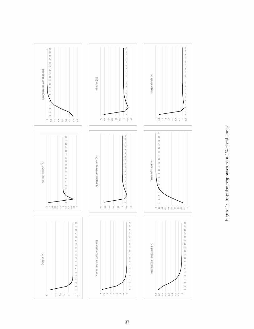
‐0.2

 

0 

0.2

 

0.4

 

0.6

 

0.8

 

1 

1.2

 

1 

2 

3 

4 

5 

6 

7 

8 

9 

10 

11 

12 

13 

14 

15 

16 

17 

18 

19 

20 

Outp

ut (%

) 

‐0.2

 

‐0.1

 

0 

0.1

 

0.2

 

0.3

 

0.4

 

0.5

 

1 

2 

3 

4 

5 

6 

7 

8 

9 

10 

11 

12 

13 

14 

15 

16 

17 

18 

19 

20 

?;;<@

;80@

 A:6B/

C19:6 23

4 

‐1 

‐0.9

 

‐0.8

 

‐0.7

 

‐0.6

 

‐0.5

 

‐0.4

 

‐0.3

 

‐0.2

 

‐0.1

 

0 

1 

2 

3 

4 

5 

6 

7 

8 

9 

10 

11 

12 

13 

14 

15 

16 

17 

18 

19 

20 

Term

s of tr

ade (%

) 

‐0.1

 

‐0.0

5 

0 

0.0

5 

0.1

 

0.1

5 

0.2

 

0.2

5 

0.3

 

1 

2 

3 

4 

5 

6 

7 

8 

9 

10 

11 

12 

13 

14 

15 

16 

17 

18 

19 

20 

56789:6 23

4 

0 

0.1

 

0.2

 

0.3

 

0.4

 

0.5

 

0.6

 

0.7

 

0.8

 

1 

2 

3 

4 

5 

6 

7 

8 

9 

10 

11 

12 

13 

14 

15 

16 

17 

18 

19 

20 

Inte

rest

 rate

 (annualise

d %

) 

‐0.8

 

‐0.7

 

‐0.6

 

‐0.5

 

‐0.4

 

‐0.3

 

‐0.2

 

‐0.1

 

0 

1 

2 

3 

4 

5 

6 

7 

8 

9 

10 

11 

12 

13 

14 

15 

16 

17 

18 

19 

20 

HEA

8<F

E86 A

:6B/

C19:6 23

4 

‐1 

‐0.8

 

‐0.6

 

‐0.4

 

‐0.2

 

0 

0.2

 

0.4

 

0.6

 

0.8

 

1 

1.2

 

1 

2 

3 

4 

5 

6 

7 

8 

9 

10 

11 

12 

13 

14 

15 

16 

17 

18 

19 

20 

Outp

ut gro

wth

 (%

) 

0 

0.5

 

1 

1.5

 

2 

2.5

 

3 

3.5

 

4 

1 

2 

3 

4 

5 

6 

7 

8 

9 

10 

11 

12 

13 

14 

15 

16 

17 

18 

19 

20 

G:6!H

EA8<F

E86 A

:6B/

C19:6 23

4 

‐0.2

 

0 

0.2

 

0.4

 

0.6

 

0.8

 

1 

1.2

 

1.4

 

1.6

 

1 

2 

3 

4 

5 

6 

7 

8 

9 

10 

11 

12 

13 

14 

15 

16 

17 

18 

19 

20 

Marg

inal co

st (%

) 

Fig

ure

1:Im

pu

lse

resp

onse

sto

a1%

fisc

alsh

ock

37

‐1.4

 

‐1.2

 

‐1 

‐0.8

 

‐0.6

 

‐0.4

 

‐0.2

 

0 

1 

2 

3 

4 

5 

6 

7 

8 

9 

10 

11 

12 

13 

14 

15 

16 

17 

18 

19 

20 

Outp

ut (%

) 

‐1.2

 

‐1 

‐0.8

 

‐0.6

 

‐0.4

 

‐0.2

 

0 

1 

2 

3 

4 

5 

6 

7 

8 

9 

10 

11 

12 

13 

14 

15 

16 

17 

18 

19 

20 

I556D

5=0D

 <7?@/

A1B7? 23

 

‐1 

‐0.9

 

‐0.8

 

‐0.7

 

‐0.6

 

‐0.5

 

‐0.4

 

‐0.3

 

‐0.2

 

‐0.1

 

0 

1 

2 

3 

4 

5 

6 

7 

8 

9 

10 

11 

12 

13 

14 

15 

16 

17 

18 

19 

20 

Term

s of tr

ade (%

) 

‐1.6

 

‐1.4

 

‐1.2

 

‐1 

‐0.8

 

‐0.6

 

‐0.4

 

‐0.2

 

0 

1 

2 

3 

4 

5 

6 

7 

8 

9 

10 

11 

12 

13 

14 

15 

16 

17 

18 

19 

20 

C?F=B7? 23

4 

0 

0.2

 

0.4

 

0.6

 

0.8

 

1 

1.2

 

1 

2 

3 

4 

5 

6 

7 

8 

9 

10 

11 

12 

13 

14 

15 

16 

17 

18 

19 

20 

Inte

rest

 rate

 (annualise

d %

) 

‐1.5

 

‐1 

‐0.5

 

0 

0.5

 

1 

1 

2 

3 

4 

5 

6 

7 

8 

9 

10 

11 

12 

13 

14 

15 

16 

17 

18 

19 

20 

Outp

ut gro

wth

 (%

) 

‐2.5

 

‐2 

‐1.5

 

‐1 

‐0.5

 

0 

1 

2 

3 

4 

5 

6 

7 

8 

9 

10 

11 

12 

13 

14 

15 

16 

17 

18 

19 

20 

K7?‐:

;<=6>

;=? <

7?@/

A1B7? 23

4 

‐3 

‐2.5

 

‐2 

‐1.5

 

‐1 

‐0.5

 

0 

1 

2 

3 

4 

5 

6 

7 

8 

9 

10 

11 

12 

13 

14 

15 

16 

17 

18 

19 

20 

Marg

inal co

st (%

) 

Fig

ure

2:Im

pu

lse

resp

onse

sto

a1%

inte

rest

rate

shock

38

0 

0.0

5 

0.1

 

0.1

5 

0.2

 

0.2

5 

0.3

 

0.3

5 

0.4

 

1 

2 

3 

4 

5 

6 

7 

8 

9 

10 

11 

12 

13 

14 

15 

16 

17 

18 

19 

20 

Outp

ut (%

) 

0 

0.0

5 

0.1

 

0.1

5 

0.2

 

0.2

5 

0.3

 

0.3

5 

1 

2 

3 

4 

5 

6 

7 

8 

9 

10 

11 

12 

13 

14 

15 

16 

17 

18 

19 

20 

45567

58/7

 9:;<.

=0>:; 12

3 

0 

0.1

 

0.2

 

0.3

 

0.4

 

0.5

 

0.6

 

1 

2 

3 

4 

5 

6 

7 

8 

9 

10 

11 

12 

13 

14 

15 

16 

17 

18 

19 

20 

Term

s of tr

ade (%

) 

‐0.4

5 

‐0.4

 

‐0.3

5 

‐0.3

 

‐0.2

5 

‐0.2

 

‐0.1

5 

‐0.1

 

‐0.0

5 

0 

0.0

5 

1 

2 

3 

4 

5 

6 

7 

8 

9 

10 

11 

12 

13 

14 

15 

16 

17 

18 

19 

20 

C;D8>:; 12

3 

‐0.7

 

‐0.6

 

‐0.5

 

‐0.4

 

‐0.3

 

‐0.2

 

‐0.1

 

0 

1 

2 

3 

4 

5 

6 

7 

8 

9 

10 

11 

12 

13 

14 

15 

16 

17 

18 

19 

20 

Inte

rest

 rate

 (annualise

d %

) 

0 

0.0

5 

0.1

 

0.1

5 

0.2

 

0.2

5 

0.3

 

0.3

5 

0.4

 

0.4

5 

1 

2 

3 

4 

5 

6 

7 

8 

9 

10 

11 

12 

13 

14 

15 

16 

17 

18 

19 

20 

HF9

86A

F8; 9

:;<.

=0>:; 12

3 

‐0.2

 

‐0.1

 

0 

0.1

 

0.2

 

0.3

 

0.4

 

1 

2 

3 

4 

5 

6 

7 

8 

9 

10 

11 

12 

13 

14 

15 

16 

17 

18 

19 

20 

Outp

ut gro

wth

 (%

) 

‐0.5

 

‐0.4

 

‐0.3

 

‐0.2

 

‐0.1

 

0 

0.1

 

0.2

 

0.3

 

1 

2 

3 

4 

5 

6 

7 

8 

9 

10 

11 

12 

13 

14 

15 

16 

17 

18 

19 

20 

K:;‐H

F986A

F8; 9

:;<.

=0>:; 12

3 

‐1.6

 

‐1.4

 

‐1.2

 

‐1 

‐0.8

 

‐0.6

 

‐0.4

 

‐0.2

 

0 

0.2

 

1 

2 

3 

4 

5 

6 

7 

8 

9 

10 

11 

12 

13 

14 

15 

16 

17 

18 

19 

20 

Marg

inal co

st (%

) 

Fig

ure

3:Im

pu

lse

resp

onse

sto

a1%

pro

du

ctiv

ity

shock

39

‐0.0

1 

0 

0.0

1 

0.0

2 

0.0

3 

0.0

4 

0.0

5 

0.0

6 

0.0

7 

0.0

8 

1 

2 

3 

4 

5 

6 

7 

8 

9 

10 

11 

12 

13 

14 

15 

16 

17 

18 

19 

20 

Outp

ut (%

) 

‐0.0

5 

0 

0.0

5 

0.1

 

0.1

5 

0.2

 

0.2

5 

1 

2 

3 

4 

5 

6 

7 

8 

9 

10 

11 

12 

13 

14 

15 

16 

17 

18 

19 

20 

H887I

860I

 <=:>/

B1C=: 23

4 

‐1.2

 

‐1 

‐0.8

 

‐0.6

 

‐0.4

 

‐0.2

 

0 

1 

2 

3 

4 

5 

6 

7 

8 

9 

10 

11 

12 

13 

14 

15 

16 

17 

18 

19 

20 

Term

s of tr

ade (%

) 

‐0.2

5 

‐0.2

 

‐0.1

5 

‐0.1

 

‐0.0

5 

0 

0.0

5 

0.1

 

0.1

5 

1 

2 

3 

4 

5 

6 

7 

8 

9 

10 

11 

12 

13 

14 

15 

16 

17 

18 

19 

20 

D:E6C=: 23

4 

‐0.3

5 

‐0.3

 

‐0.2

5 

‐0.2

 

‐0.1

5 

‐0.1

 

‐0.0

5 

0 

0.0

5 

1 

2 

3 

4 

5 

6 

7 

8 

9 

10 

11 

12 

13 

14 

15 

16 

17 

18 

19 

20 

Inte

rest

 rate

 (annualise

d %

) 

‐0.0

5 

0 

0.0

5 

0.1

 

0.1

5 

0.2

 

0.2

5 

1 

2 

3 

4 

5 

6 

7 

8 

9 

10 

11 

12 

13 

14 

15 

16 

17 

18 

19 

20 

@9<

67A

96: <

=:>/

B1C=: 23

4 

‐0.0

6 

‐0.0

4 

‐0.0

2 

0 

0.0

2 

0.0

4 

0.0

6 

0.0

8 

1 

2 

3 

4 

5 

6 

7 

8 

9 

10 

11 

12 

13 

14 

15 

16 

17 

18 

19 

20 

Outp

ut gro

wth

 (%

) 

‐0.0

5 

0 

0.0

5 

0.1

 

0.1

5 

0.2

 

0.2

5 

0.3

 

1 

2 

3 

4 

5 

6 

7 

8 

9 

10 

11 

12 

13 

14 

15 

16 

17 

18 

19 

20 

?=:‐@

9<67A

96: <

=:>/

B1C=: 23

4 

‐0.0

4 

‐0.0

2 

0 

0.0

2 

0.0

4 

0.0

6 

0.0

8 

0.1

 

0.1

2 

1 

2 

3 

4 

5 

6 

7 

8 

9 

10 

11 

12 

13 

14 

15 

16 

17 

18 

19 

20 

Marg

inal co

st (%

) 

Fig

ure

4:Im

pu

lse

resp

onse

sto

a1%

wor

ldou

tpu

tsh

ock

40

Figure 5: Cumlative fiscal multiplier for a 1% fiscal shock

Figure 6: Observed output growth from the data (demeaned)

Figure 7: Observed G(t)/Y(t) ratio from the data

41

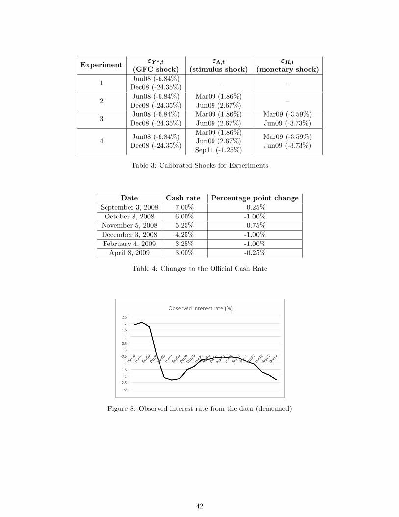
ExperimentεY ∗,t

(GFC shock)εΛ,t

(stimulus shock)εR,t

(monetary shock)

1Jun08 (-6.84%)Dec08 (-24.35%)

– –

2Jun08 (-6.84%)Dec08 (-24.35%)

Mar09 (1.86%)Jun09 (2.67%)

–

3Jun08 (-6.84%)Dec08 (-24.35%)

Mar09 (1.86%)Jun09 (2.67%)

Mar09 (-3.59%)Jun09 (-3.73%)

4Jun08 (-6.84%)Dec08 (-24.35%)

Mar09 (1.86%)Jun09 (2.67%)Sep11 (-1.25%)

Mar09 (-3.59%)Jun09 (-3.73%)

Table 3: Calibrated Shocks for Experiments

Date Cash rate Percentage point change

September 3, 2008 7.00% -0.25%

October 8, 2008 6.00% -1.00%

November 5, 2008 5.25% -0.75%

December 3, 2008 4.25% -1.00%

February 4, 2009 3.25% -1.00%

April 8, 2009 3.00% -0.25%

Table 4: Changes to the Official Cash Rate

Figure 8: Observed interest rate from the data (demeaned)

42

Exp

erim

ent

1

Exp

erim

ent

2

Fig

ure

9:

Exp

erim

ents

1(G

FC

shock

s)an

d2

(GF

Can

dfi

scal

shock

s)

43

Exp

erim

ent

2

Exp

erim

ent

3

Fig

ure

10:

Exp

erim

ents

2(G

FC

and

fisc

alsh

ock

s)an

d3

(GF

C,

fisc

alan

dm

onet

ary

shock

s)

44

Exp

erim

ent

3

Exp

erim

ent

4

Fig

ure

11:

Exp

erim

ents

3(G

FC

,fi

scal

and

mon

etar

ysh

ock

s)an

d4

(plu

sn

egat

ive

fisc

alsh

ock

inm

ediu

mru

n)

45