ECONOMIC GROWTH CENTER

YALE UNIVERSITY

P.O. Box 208629New Haven, CT 06520-8269

http://www.econ.yale.edu/~egcenter/

CENTER DISCUSSION PAPER NO. 893

EFFECTIVE LABOR REGULATIONAND MICROECONOMIC FLEXIBILITY

Ricardo J. CaballeroMIT

Devin N. CowanInter-American Development Bank

Eduardo M.R.A. EngelYale University

Alejandro MiccoInter-American Development Bank

September 2004

Notes: Center Discussion Papers are preliminary materials circulated to stimulate discussions andcritical comments.

We thank Joseph Altonji, John Haltiwanger, Michael Keane, Norman Loayza andparticipants at the LACEA 2003 conference for useful comments. Caballero thanks the NSFfor financial support.

This paper can be downloaded without charge from the Social Science Research Network electroniclibrary at: http://ssrn.com/abstract=581021

An index to papers in the Economic Growth Center Discussion Paper Series is located at: http://www.econ.yale.edu/~egcenter/research.htm

Effective Labor Regulation and Microeconomic Flexibility

Ricardo J. CaballeroKevin N. Cowan

Eduardo M.R.A. EngelAlejandro Micco

Abstract

Microeconomic flexibility, by facilitating the process of creative-destruction, is at the coreof economic growth in modern market economies. The main reason for why this process is notinfinitely fast is the presence of adjustment costs, some of them technological, others institutional.Chief among the latter is labor market regulation. While few economists would object to such aview, its empirical support is rather weak. In this paper we revisit this hypothesis and find strongevidence for it. We use a new sectoral panel for 60 countries and a methodology suitable for sucha panel. We find that job security regulation clearly hampers the creative-destruction process,especially in countries where regulations are likely to be enforced. Moving from the 20th to the 80th

percentile in job security, in countries with strong rule of law, cuts the annual speed of adjustmentto shocks by a third while shaving off about one percent from annual productivity growth. The samemovement has negligible effects in countries with weak rule of law.

Keywords: Microeconomic rigidities, creative-destruction, job security regulation, adjustmentcosts, rule of law, productivity growth

JEL Codes: E24, J23, J63, J64, K00

1 Introduction

Microeconomic flexibility, by facilitating the ongoing process of creative-destruction, is at the core of eco-

nomic growth in modern market economies. This basic idea has been with economists for centuries, was

brought to the fore by Schumpeter fifty years ago, and has recently been quantified in a wide variety of con-

texts.1 In US Manufacturing, for example, more than half of aggregate productivity growth can be directly

linked to this process.2

The main obstacle faced by microeconomic flexibility is adjustment costs. Some of these costs are

purely technological, others are institutional. Chief among the latter is labor market regulation, in partic-

ular job security provisions. The literature on the impact of labor market regulation on the many different

economic, political and sociological variables associated to labor markets and their participants is extensive

and contentious. However, the proposition that job security provisions reduce restructuring is a point of

agreement.

Despite this consensus, the empirical evidence supporting the negative impact of labor market regulation

on microeconomic flexibility has been scant at best. This is not too surprising, as the obstacles to empiri-

cal success are legions, including poor measurement of restructuring activity and labor market institutions

variables, both within a country and more so across countries. In this paper we make a new attempt. We

develop a methodology that allows us to bring together the extensive new data set on labor market regula-

tion constructed by Djankov et al. (2003) with comparable cross-country cross-sectoral data on employment

and output from the UNIDO (2002) data-set. We also emphasize the key distinction betweeneffectiveand

official labor market regulation.

The methodology builds on the simple partial-adjustment idea that larger adjustment costs are reflected

in slower employment adjustment to shocks.3 The accumulation of limited adjustment to these shocks

builds a wedge between frictionless and actual employment, which is the main right hand side variable in

this approach. We propose a new way of estimating this wedge, which allows us to pool data on labor market

legislation with comparable employment and output data for a broad range of countries. As a result, we are

able to enlarge the effective sample to 60 economies, more than double the country coverage of previous

studies in this literature.4 Our attempt to measureeffectivelabor regulation interacts existing measures of

job security provision with measures of rule of law and government efficiency.

Our results are clear and robust: countries with less effective job security legislation adjust more quickly

to imbalances between frictionless and actual employment. In countries with strong rule of law, moving

from the 20th to the 80th percentile of job security lowers the speed of adjustment to shocks by 35 percent

and cuts annual productivity growth by0.86percent. The same movement for countries with low rule of law

1See, e.g., the review in Caballero and Hammour (2000).2See, e.g., Foster, Haltiwanger and Krizan (1998).3For surveys of the empirical literature on partial-adjustment see Nickell (1986) and Hammermesh (1993).4To our knowledge, the broadest cross-country study to date – Nickell and Nuziata (2000) – included 20 high income OECD

countries. Other recent studies, such as Burgess and Knetter (1998) and Burgess et al. (2000), pool industry-level data from 7OECD economies.

1

only reduces the speed of adjustment by approximately 1 percent and productivity growth by 0.02 percent.

The paper proceeds as follows. Section 2 presents the methodology and describes the new data set.

Section 3 discusses the main results and explores their robustness. Section 4 gauges the impact of effective

labor protection on productivity growth. Section 5 concludes.

2 Methodology and Data

2.1 Methodology

2.1.1 Overview

The starting point for our methodology is a simple adjustment hazard model, where the change in the

number of (filled) jobs in sectorj in countryc between timet − 1 andt is a probabilistic (at least to the

econometrician) function of the gap between desired and actual employment:

∆ejct = ψ jctGapjct Gapjct ≡ e∗jct −ejc,t−1, (1)

whereejct ande∗jct denote the logarithm of employment and desired employment, respectively. The random

variableψ jct , which is assumed i.i.d. both across sectors and over time, takes values in the interval[0,1] and

has country-specific meanλc and varianceωcλc(1−λc), with 0≤ ωc ≤ 1. The caseωc = 0 corresponds

to the standard quadratic adjustment model, the caseωc = 1 to the Calvo (1983) model. The parameter

λc captures microeconomic flexibility. Asλc goes to one, all gaps are closed quickly and microeconomic

flexibility is maximum. Asλc decreases, microeconomic flexibility declines.

Equation (1) hints at two important components of our methodology: We need to find a measure of

the employment gap and a strategy to estimate the average (overj and t) speeds of adjustment (theλc).

We describe both ingredients in detail in what follows. In a nutshell, we construct estimates ofe∗jct , the

only unobserved element of the gap, by solving the optimization problem of a sector’s representative firm,

as a function of observables such as labor productivity and a suitable proxy for the average market wage.

We estimateλc from (1), based upon the large cross-sectional size of our sample and the well documented

heterogeneity in the realizations of the gaps and theψ jct ’s (see, e.g., Caballero, Engel and Haltiwanger

(1997) for US evidence).

2.1.2 Details

Output and demand for a sector’s representative firm are given by:

y = a+αe+βh, (2)

p = d− 1η

y, (3)

2

wherey, p, e, a, h, d denote output, price, employment, productivity, hours worked and demand shocks, and

η is the price elasticity of demand. We letγ ≡ (η−1)/η, with η > 1, 0 < α < 1, 0 < β < 1 andγ < 1/α.

All variables are in logs.

Firms are competitive in the labor market but pay wages that increase with the number of hours worked:

w = ko + log(Hµ+Ω).

This can be approximated by:

w = wo +µ(h−h), (4)

with wo andµ determined byko andΩ, andh constant over time and interpreted below. In order to ensure

interior solutions, we assumeαµ> β andµ> βγ.

A key assumption is that the representative firm within each sector only faces adjustment costs when it

changes employment levels, not when it changes the number of hours worked (beyond overtime payments).5

It follows that the sector’s choice of hours in every period can be expressed in terms of its current level of

employment, by solving the corresponding first order condition for hours.

In a frictionless labor market the firm’s employment level also satisfies a simplestaticfirst order condi-

tion for employment. Our functional forms then imply that the optimal choice of hours,h, does not depend

on the employment level. A patient calculation shows that

h =1µ

log

(βΩ

αµ−β

).

We denote the corresponding employment level byeand refer to it as thestatic employment target:

e= C+1

1−αγ[d+ γa−wo],

with C a constant that depends onµ, α, β andγ.

The following relation between the employment gap and the hours gap then follows:

e−e =µ−βγ1−αγ

(h−h). (5)

This is the expression used by Caballero and Engel (1993). It is not useful in our case, since we do

not have information on worked hours. Yet the argument used to derive (5) also can be used to express the

employment gap in terms of the marginal labor productivity gap:

e−e =φ

1−αγ(v−wo),

wherev denotes marginal productivity,φ ≡ µ/(µ−βγ) is decreasing in the elasticity of the marginal wage

5For evidence on this see Sargent (1978) and Shapiro (1986).

3

schedule with respect to average hours worked,µ− 1, andwo was defined in (4). Note thate− e is the

difference between the static targeteand realized employment, not the dynamic employment gape∗jct −ejct

related to the term on the right hand side of (1). However, if we assume thatd+ γa−wo follows a random

walk (possibly with an exogenously time varying drift) —an assumption consistent with the data6 — we

have thate∗jct is equal toejct plus a constantδct. It follows that

e∗jct −ejct−1 =φ

1−αγ j

(v jct −wo

jct

)+∆ejct +δct, (6)

where we have allowed for sector-specific differences inγ. Note that both marginal product and wages are

in nominal terms. However, since these expressions are in logs, their difference eliminates the aggregate

price level component.

We estimate the marginal productivity of labor,v jct , using output per worker multiplied by an industry-

level labor share, assumed constant whithin income groups and over time.

Two natural candidates to proxy forwojct are the average (across sectors within a country, at a given

point in time) of either observed wages or observed marginal productivities. The former is consistent with a

competitive labor market, the latter may be expected to be more robust in settings with long-term contracts

and multiple forms of compensation, where the salary may not represent the actual marginal cost of labor.7

We performed estimations using both alternatives and found no discernible differences (see below). This

suggests that statistical power comes mainly from the cross-section dimension, that is, from the well docu-

mented and large magnitude of sector-specific shocks. In what follows we report the more robust alternative

and approximatewo by the average marginal productivity, which leads to:

e∗jct −ejct−1 =φ

1−αγ j(v jct −v·ct)+∆ejct +δct ≡ Gapjct +δct, (7)

wherev·ct denotes the average, overj, of v jct , and we use this convention for other variables as well. The

expression above ignores systematic variations in labor productivity across sectors within a country, for

example, because (unobserved) labor quality may differ systematically across sectors. The presence of

such heterogeneity would tend to bias estimates of the speed of adjustment downward. To incorporate this

possibility we subtract from(v jct−v·ct) in (7) a moving average of relative sectoral productivity,θ jct , where

θ jct ≡ 12[(v jct−1−v·ct−1) + (v jct−2−v·ct−2)].

As a robustness check, for our main specifications we also computedθ jct using a three and four periods

moving average, without significant changes in our results (more on this when we check robustness in

6Pooling all countries and sectors together, the first order autocorrelation of the measure of∆e∗jct constructed below is−0.018.Computing this correlation by country the mean value is 0.011 with a standard deviation of 0.179.

7While we have assumed a simple competitive market for the base salary (salary for normal hours) within each sector, ourprocedure could easily accommodate other, more rent-sharing like, wage setting mechanisms (with a suitable reinterpretation ofsome parameters, but notλc).

4

Section 3.2). The resulting expression for the estimated employment-gap is:

e∗jct −ejct−1 =φ

1−αγ j(v jct − θ jct −v·ct)+∆ejct +δct ≡ Gapjct +δct, (8)

whereαγ j is constructed using the sample median of the labor share for sector j across year and income

groups.

Rearranging (8), we estimateφ from

∆ejct = − φ1−αγ j

(∆v jct −∆v·ct)+κct +υit +∆e∗jct ≡ −φzjct +κct + ε jct , (9)

where κ is a country-year dummy,∆e∗jct is the change in the desired level of employment andzjct ≡(∆v jct −∆v·ct)/(1−αγ j). We assume that changes in sectoral labor composition are negligible between

two consecutive years. In order to avoid the simultaneity bias present in this equation (∆v and ∆e∗ are

clearly correlated) we estimate (9) using(∆w jct−1−∆w·ct−1) as an instrument for(∆v jct −∆v·ct).8 Table 1

reports the estimation results of (9) for the full sample of countries and across income groups. The first two

columns use the full sample, with and without two percent of extreme values for the independent variable,

respectively. The remaining columns report the estimation results for each of our three income groups and

job security groups (more on both of these measures in Section 2.2). Based on our results for the baseline

case, we set the value ofφ at its full sample estimate of0.4 for all countries in our sample.

It is important to point out that our methodology has some advantages over standard partial adjustment

estimations. First, it summarizes in a single variable all shocks faced by a sector. This feature allows us to

increase precision and to study the determinants of the speed of adjustment using interaction terms. Second,

and related, it only requires data on nominal output and employment, two standard and well-measured

variables in most industrial surveys. Most previous studies on adjustment costs required measures of real

output or an exogenous measure of sector demand.9

2.1.3 Regressions

The central empirical question of the present study is how cross-country differences in job security regulation

affect the speed of adjustment. Accordingly, from (1) and (8) it follows that the basic equation we estimate

is:

∆ejct = λct(Gapjct +δct), (10)

8We lag the instrument to deal with the simultaneity problem and use the wage rather than productivity to reduce the (potential)impact of measurement error bias.

9Abraham and Houseman (1994), Hammermesh (1993), and Nickel and Nunziata (2000)) evaluate the differential response ofemployment to observed real output. A second option is to construct exogenous demand shocks. Although this approach overcomesthe real output concerns, it requires constructing an adequate sectorial demand shock for every country. A case in point are thepapers by Burgess and Knetter (1998) and Burgess et al. (2000), which use the real exchange rate as their demand shock. Theestimated effects of the real exchange rate on employment are usually marginally significant, and often of the opposite sign thanexpected.

5

where∆ejct is the log change in employment andλct denotes the speed of adjustment. We assume that the

latter takes the form:

λct = λ1 +λ2JSeffct , (11)

whereJSeffct is a measure ofeffectivejob security regulation. In practice we observe job security regulation

(imperfectly), but not the rigor with which it is enforced. We proxy the latter with a “rule of law” variable,

so that

JSeffct = JSct(1+aRLct), (12)

wherea is a constant andRLct is a standard measure of rule of law (see below). Substituting this expression

in (11) and the resulting expression forλct in (10), yields our main estimating equation:

∆ejct = λ1 Gapjct +λ2(Gapjct ×JSct

)+λ3

(Gapjct ×JSct×RLct

)+ δct + ε jct , (13)

with λ3 = aλ2 andδct denotes country×time fixed effects (proportional to theδct defined above).

The main coefficients of interest areλ2 andλ3, which measure how the speed of adjustment varies across

countries depending on their labor market regulation (bothde jureandde facto).

2.2 The Data

This section describes our sample and main variables. Additional variables are defined as we introduce them

later in the text.

2.2.1 Job Security and Rule of Law

We use two measures of job security, or legal protection against dismissal: the job security index constructed

by Djankov et al. (2003) for 60 countries world-wide (henceforthJSc) and the job security index constructed

by Heckman and Pages (2000) for 24 countries in OECD and Latin America (henceforthHPct). TheJSc

measure is available for a larger sample of countries and includes a broader range of job security variables.

TheHPct measure has the advantage of having time variation.

Our main job security index,JSc, is the sum of four variables, measured in 1997, each of which takes

on values between 0 and 1:(i) grounds for dismissal protectionPGc, (ii) protection regarding dismissal

proceduresPPc, (iii ) notice and severance paymentsPSc, and(iv) protection of employment in the constitu-

tion PCc. The rules on grounds of dismissal range from allowing the employment relation to be terminated

by either party at any time (employment at will) to allowing the termination of contracts only under a very

narrow list of “fair” causes. Protective dismissal procedures require employers to obtain the authorization

of third parties (such as unions and judges) before terminating the employment contract. The third vari-

able, notice and severance payment, is the one closest to theHPct measure, and is the normalized sum of

two components: mandatory severance payments after 20 years of employment (in months) and months of

advance notice for dismissals after 20 years of employment(NStc = bct+20+SPct+20, t = 1997). The four

6

components ofJSc described above increase with the level of job security.

The Heckman and Pages measure is narrower, including only those provisions that have a direct impact

on the costs of dismissal. To quantify the effects of this legislation, they construct an index that computes

the expected (at hiring) cost of a future dismissal. The index includes both the costs of advanced notice

legislation and firing costs, and is measured in units of monthly wages.

Our estimations also adjust for the level of enforcement of labor legislation. We do this by including

measures of rule of lawRLc and government efficiencyGEc from Kaufmann at al. (1999), and interact them

with JSc andHPct.10 We expect labor market legislation to have a larger impact on adjustment costs in

countries with a stronger rule of law (higherRLc) and more efficient governments (higherGEc).

The institutional variables as well as the countries in our sample and their corresponding income group

are reported in Table 2. Table 3 reports the sample correlations between our main cross-country variables

and summary statistics for each of these measures for three income groups (based on World Bank per capita

income categories).11 As expected, the correlation between the two measures of job security is positive and

significant. Differences can be explained mainly by the broader scope of theJSct index. Also as expected,

rule of law and government efficiency increase with income levels. Note, however, that neither measure of

job security is positively correlated with income per capita, since bothJSct andHPc are highest for middle

income countries.

2.2.2 Industrial Statistics

Our output, employment and wage data come from the 2002 3-digit UNIDO Industrial Statistics Database.

The UNIDO database contains data for the period 1963-2000 for the 28 manufacturing sectors that corre-

spond to the 3 digit ISIC code (revision 2). Because our measures of job security and rule of law are time

invariant and measured in recent years, however, we restrict our sample to the period 1980-2000. Data on

output and labor compensation are in current US dollars (inflation is removed through time effects in our

regressions). Throughout the paper our main dependent variable is∆ejct , the log change in total employment

in sectorj of countryc in periodt.

A large number of countries are included in the original dataset — however our sample is constrained

by the cross-country availability of the independent variables measuring job security. In addition, we drop

two percent of extreme employment changes in each of the three income groups. For our main specification

the resulting sample includes 60 economies. Table 3 shows descriptive statistics for the dependent variable

by income group.

10For rule of law and government efficiency we use the earliest value available in the Kaufmann et al. (1999) database: 1996,since this is closest to the Djankov et al. (2003) measure, which is for 1997.

11Income groups are: 1=High Income OECD, 2=High Income Non OECD and Upper Middle Income, 3=Lower Middle Incomeand Low Income.

7

3 Results

This section presents our main result, showing that effective job security has a significant negative effect on

the speed of adjustment of employment to shocks in the employment-gap. It also presents several robustness

exercises.

3.1 Main results

Recall that our main estimating equation is:

∆ejct = λ1 Gapjct +λ2(Gapjct ×JSc

)+λ3

(Gapjct ×JSc×RLc

)+ δct + ε jct . (14)

Note that we have dropped time subscripts fromJSc andRLc as we only use time invariant measures of

rule of law and job security in our baseline estimation. Note also that in all specifications that include the

(Gapict ×JSct×RLc) interaction we also include the respectiveGapict ×RLc as a control variable.

We start by ignoring the effect of job security on the speed of adjustment, and setλ2 and λ3 equal

to zero. This gives us an estimate of the average speed of adjustment and is reported in column 1 of

Table 4. On average (across countries and periods) we find that 60% of the employment-gap is closed in

each period. Furthermore, our measure of the employment-gap and country×year fixed effects explain 60%

of the variance in log-employment growth.

The next three columns present our main results, which are repeated in columns 5 to 7 allowing for

different λ1 by sectors and country income level.12 Column 2 (and 5) presents our estimate ofλ2. This

coefficient has the right sign and is significant at conventional confidence levels. Employment adjusts more

slowly to shocks in the employment-gap in countries with higher levels of official job security.

Next, we allow for a distinction between effective and official job security. Results are reported in

columns 3 and 4 (and, correspondingly, 6 and 7) for different rules-enforcement criteria. In columns 3 and

6 the distinction between effective and official job security is captured by the product ofJSc andDSRLc,

whereDSRLc is a dummy variable for countries with strong rule of law (RLc≥RLGreece— where Greece is

the OECD country with the lowest RL score). The three panels in Figure 1 show the value of the job security

index for countries in the high, medium and low income groups, respectively. Nowλ2 becomes insignificant,

while λ3 has the right sign and is highly significant. That is, the same change inJSc will have a significantly

larger (downward) effect on the speed of adjustment in countries with stricter enforcement of laws, as

measured by our rule-of-law dummy. The effect of the estimated coefficients reported in column 3 is large.

In countries with strong rule of law, moving from the 20th percentile of job security(−0.19) to the 80th

percentile(0.23) reducesλ by 0.22. The same change in job security legislation has a considerable smaller

effect, 0.006, on the speed of adjustment in the group of economies with weak rule of law. Employment

12We allow for an interaction betweenGapjct and 3 digit ISIC sector dummies (we also include sector fixed effects). We alsocontrol for the possibility that our results are driven by omitted variables, correlated with our measures of job security. For this, weinclude an additional interaction betweenGapjct and three income-group dummies.

8

adjusts more slowly to shocks in the employment-gap in countries with higher levels of effective job security.

Columns 4 and 7 address whether the negative coefficient onλ3 is robust to other measures of legal

enforcement. To do so we use an alternative variable from the Kaufmann et al. (1999) dataset – government

effectiveness (GE) – and construct a dummy variable for high effectiveness countries (GEc ≥GEGreece).

Clearly, the results are very close to those reported in columns 3 and 7. Job security legislation has a

significant negative effect on the estimated speed of adjustment when governments are effective – a proxy

for enforcement of existing labor regulation.

Finally, the last column in Table 4 uses an alternative measure of job security. We repeat our specification

from column 7 (including sector and income dummies) using the Heckman-Pages (2000) measure of job

security. TheHPct data are only available for countries in the OECD and Latin America so our sample

size is reduced by half, and most low income countries are dropped. The flip side is that this measure is

time varying which potentially allows us to capture the effects of changes in the job security regulation. As

reported in column 8, we find a negative and significant effect ofHPct on the speed of adjustment.

3.2 Further robustness

We continue our robustness exploration by assessing the impact of three broad econometric issues: alterna-

tive gap-measures, exclusion of potential (country) outliers, and misspecification due to endogeneity of the

gap measure.

3.2.1 Alternative gap-measures

Table 4 suggests that conditional on our measure of the employment-gap, our main findings are robust: job

security, when enforced, has a significant negative impact on the speed of adjustment to the employment-gap.

Table 5 tests the robustness of this result to alternative measures of the employment-gap. Columns 1 and 2

relax the assumption of aφ common across all countries. They repeat our baseline specifications —columns

2 and 3 in Table 4— using the values ofφ estimated per income-group reported in Table 1. In turn, columns

3 and 4 report the results of using values ofφ estimated across countries grouped by level of job security.13

Next, columns 5 through 8 repeat our baseline specifications using a three and four period moving average

to estimateθ jct . The final two columns (9 and 10) use an alternative specification forwojct based on average

wages instead of average productivity (see equation 8) to buildGapjct . In all of the specifications reported

in Table 5, our results remain qualitatively the same as in Table 4.

3.2.2 Exclusion of potential (country) outliers

Table 6 reports estimates ofλ2 andλ3 using the specification from column 3 in Table 4 but dropping one

country from our sample at a time. In all cases the estimated coefficient onλ3 is negative and significant at

conventional confidence intervals.13Countries are grouped into the upper, middle and lower thirds of job security.

9

However, it is also apparent in this table that excluding either Hong Kong or Kenya makes a substantial

difference in the point estimates. For this reason, we re-estimate our model from scratch (that is, fromφup) now excluding these two countries. In this case the value ofφ rises from 0.40 to 0.42. Qualitatively,

however, the main results remain unchanged. Table 7 reports these results.

3.2.3 Potential endogeneity of the gap measure

One concern with our procedure is that the construction of the gap measure includes the change in employ-

ment. While this does not represent a problem under the null hypothesis of the model, any measurement

error in employment andφzjt could introduce important biases. We address this issue with two procedures.

Before describing these procedures, we note that the standard solution of passing the∆e-component of

the gap defined in (8) to the left hand side of the estimating equation (10) does not work in our context.

Passing∆e to the left suggests that the coefficient on the resulting gap will be equal toλ/(1− λ). As

shown in Appendix A, this holds only in the case of a partial adjustment model (ω = 0 in the notation of

Section 2.1). By contrast, in the case of a Calvo-type adjustment (ω = 1), the corresponding coefficient will,

on average, be negative.14 More important, even small departures from a partial adjustment model (small

values ofω) introduce significant biases when estimatingλ using this approach.

Next we turn to the two procedures. The first procedure maintains our baseline specification, but in-

struments for the contemporaneous gap measure. Given thatGapjct = φzjt + ∆ejct can be rewritten as

φzj,t−1 + ∆e∗jct , a natural instrument is the lag of the ex-post gap,φzjc,t−1. Unfortunately, the latter is not a

valid instrument if it is computed with measurement error and this error is serially correlated. In our speci-

fication this could be the case because we use a moving average to construct the estimate of relative sectoral

productivity,θ jct . To avoid this problem, we construct an alternative measure of the ex-post gap letting wage

data play the role of productivity data when calculating thev andθ terms on the right hand side of (8).

The second procedure re-writes the model in a standard dynamic panel formulation that removes the

contemporaneous employment change from the right hand side:15

∆Gapjct = (1−λc)∆Gapjct−1 + ε jct . (15)

Table 8 reports the values of the averageλ estimated with these two alternative, and much less precise,

procedures. For comparison purposes, the first row reproduces the first column in Table 4. The second row

shows the result for the IV procedure based on using lagged wages as instruments. Finally, Row 3 reports

the estimate from the dynamic panel. It is apparent from the table that the estimates of averageλ are in the

right ballpark, and hence we conclude that the bias due to a potentially endogenous gap is not significant.

14In the Calvo-case, for every observation either the (modified) gap or the change in employment is zero. The former happenswhen adjustment takes place, the latter when it does not. It follows that the covariance of∆eand the (modified) gap will be equal tominus the product of the mean of both variables. Since these means have the same sign, the estimated coefficient will be negative.See Appendix A for a formal derivation.

15To estimate this equation we follow Anderson and Hsiao (1982) and use twice and three-times lagged values of∆Gapjct asinstruments for the RHS variable. Similar results are obtained if we follow Arellano and Bond (1991).

10

4 Gauging the Costs of Effective Labor Protection

By impairing worker movements from less to more productive units, effective labor protection reduces ag-

gregate output and slows down economic growth. In this section we develop a simple framework to quantify

this effect. Any such exercise requires strong assumptions and our approach is no exception. Nonetheless,

our findings suggest that the costs of the microeconomic inflexibility caused by effective protection is large.

In countries with strong rule of law, moving from the 20th to the 80th percentile of job security lowers an-

nual productivity growth somewhere between 0.9 and 1.2 percent. The same movement for countries with

low rule of law has a negligible impact on TFP.

Consider a continuum of establishments, indexed byi, that adjust labor in response to productivity

shocks, while their share of the economy’s capital remains fixed over time. Their production functions

exhibit constant returns to (aggregate) capital,Kt , and decreasing returns to labor:

Yit = Bit KtLαit , (16)

whereBit denotes plant-level productivity and0 < α < 1. TheBit ’s follow geometric random walks, that

can be decomposed into the product of a common and an idiosyncratic component:

∆ logBit ≡ bit = vt +vIit ,

where thevt are i.i.d.N (µA,σ2A) and thevit ’s are i.i.d. (across productive units, over time and with respect to

the aggregate shocks)N (0,σ2I ). We setµA = 0, since we are interested in the interaction between rigidities

and idiosyncratic shocks, not in Jensen-inequality-type effects associated with aggregate shocks.

The price-elasticity of demand isη > 1. Aggregate labor is assumed constant and set equal to one. We

defineaggregate productivity, At , as:

At =Z

Bit Lαit di, (17)

so that aggregate output,Yt ≡R

Yit di, satisfies

Yt = AtKt .

Units adjust with probabilityλc in every period, independent of their history and of what other units

do that period.16 The parameter that captures microeconomic flexibility isλc. Higher values ofλc are

associated with a faster reallocation of workers in response to productivity shocks.

Standard calculations show that the growth rate of output,gY, satisfies:

gY = sA−δ, (18)

16More precisely, whether uniti adjusts at timet is determined by a Bernoulli random variableξit with probability of successλc,where theξit ’s are independent across units and over time. This corresponds to the caseω = 1 in Section 2.1.

11

wheresdenotes the savings rate (assumed exogenous) andδ the depreciation rate for capital.

Now compare two economies that differ only in their degree of microeconomic flexibility,λc,1 < λc,2.

Tedious but straightforward calculations relegated to Appendix B show that:

gY,2−gY,1 ' (gY,1 +δ)[

1λc,1

− 1λc,2

]θ, (19)

with

θ =αγ(2−αγ)2(1−αγ)2 σ2,

γ = (η−1)/η, σ2 = σ2I +σ2

A.17

We choose parameters to apply (19) as follows: The mark-up is set at 20% (so thatγ = 5/6), gY,1 to the

average rate of growth per worker in our sample for the 1980-1990 period, 0.7%,σ = 27%,18 α = 2/3, and

δ = 6%.

Table 9 reports estimated speeds of adjustment across countries. Table 10 reports the average annual

productivity costs of the deviation between each quintile and the bottom quintile in estimated speed of

adjustment. These numbers are large. More important, they imply that moving from the 20th to the 80th

percentile in job security, in countries with strong rule of law, reduces annual productivity growth by0.86%.

The same change in job security legislation has a much smaller effect on TFP growth, 0.02%, in the group

of economies with weak rule of law.

We are fully aware of the many caveats that such ceteris-paribus comparison can raise, but the point of

the table is to provide an alternative metric of the potential significance of observed levels of effective labor

protection. Moreover, these numbers are roughly consistent with what we obtain when running a regression

of productivity growth on the estimatedλc’s for all the economies in our sample from 1980 to 1990 (see

Table 11 and Figure 2). Focusing on the results controlling for income groups (column 3), the coefficient on

λc is around 0.05 and significant at the 1 percent level. Combining these estimates with those in Column 3

of Table 4 implies that when moving from the 20th to the 80th percentile in job security, annual TFP growth

falls by as much as 1.18% in countries with high rule of law. In contrast, a similar improvement in labor

regulation in countries with low rule law reduces TFP growth by only 0.03%.

5 Concluding Remarks

Many papers have shown that, in theory, job security regulation depresses firm level hiring and firing de-

cisions. Job security provisions increase the cost of reducing employment and therefore lead to fewer dis-

17There also is a (static) jump in the level of aggregate productivity whenλ increases, given by:

A2−A1

A1'

[1λ1− 1

λ2

]θ.

See Appendix B for the proof.18This is the average across the five countries considered in Caballero et al. (2004).

12

missals when firms are faced with negative shocks. Conversely, when faced with a positive shock, the

optimal employment response takes into account the fact that workers may have to be fired in the future, and

the employment response is smaller. The overall effect is a reduction of the speed of adjustment to shocks.

However, conclusive empirical evidence on the effects of job security regulation has been elusive. One

important reason for this deficit has been the lack of information on employment regulation for a sufficiently

large number of economies that can be integrated to cross sectional data on employment outcomes. In this

paper we have developed a simple empirical methodology that has allowed us to fill some of the empiri-

cal gap by exploiting: (a) the recent publication of two cross-country surveys on employment regulations

(Heckman and Pages (2000) and Djankov et al. (2003)) and, (b) the homogeneous data on employment and

production available in the UNIDO dataset. Another important reason for the lack of empirical success is

differences in the degree of regulation enforcement across countries. We address this problem by interacting

the measures of employment regulation with different proxies for law-enforcement.

Using a dynamic labor demand specification we estimate the effects of job security across a sample of

60 countries for the period from 1980 to 1998. We consistently find a relatively lower speed of adjustment

of employment in countries with high legal protection against dismissal, especially when such protection is

likely to be enforced.

13

References

[1] Abraham, K. and S. Houseman (1994). “Does Employment Protection Inhibit Labor Market Flexibil-

ity: Lessons From Germany, France and Belgium.” In: R.M. Blank, editor,Protection Versus Economic

Flexibility: Is There A Tradeoff?. Chicago: University of Chicago Press.

[2] Anderson, T.W. and C. Hsiao (1982). “Formulation and Estimation of Dynamic Models Using Panel

Data,”Journal of Econometrics, 18, 67–82.

[3] Arellano, M. and S.R. Bond (1991). “Some Specification Tests for Panel Data: Montecarlo Evidence

and an Application to Employment Equations,”Review of Economic Studies, 58, 277-298.

[4] Barro, R.J. and J.W. Lee (1996). “International Measures of Schooling Years and Schooling Quality,”

American Economic Review, Papers and Proceedings, 86, 218–223.

[5] Burgess. S. and M. Knetter (1998). “An International Comparison of Eployment Adjustment to Ex-

change Rate Fluctuations.”Review of International Economics.6(1): 151-163.

[6] Burgess, S., M. Knetter and C. Michelacci (2000). “Employment and Output Adjustment in the OECD:

A Disaggregated Analysis of the Role of Job Security Provisions.”Economica67: 419-435.

[7] Caballero R. and E. Engel (1993). “Microeconomic Adjustment Hazards and Aggregate Dynamics.”

Quarterly Journal of Economics.108(2): 359-83.

[8] Caballero R., E. Engel, and J. Haltiwanger (1997), “Aggregate Employment Dynamics: Building from

Microeconomic Evidence,”American Economic Review87(1), 115–137.

[9] Caballero R., E. Engel, and A. Micco (2004), “Microeconomic Flexibility in Latin America,” NBER

Working Paper No. 10398.

[10] Caballero, R. and M. Hammour (2000). “Creative Destruction and Development: Institutions, Crises,

and Restructuring,”Annual World Bank Conference on Development Economics 2000, 213-241.

[11] Calvo, G (1983). “Staggered Prices in a Utility Maximizing Framework.”Journal of Monetary Eco-

nomics.12: 383-98.

[12] Djankov, S., R. La Porta, F. Lopez-de-Silanes, A. Shleifer and J. Botero (2003). “The Regulation of

Labor.” NBER Working Paper No. 9756.

[13] Foster L., J. Haltiwanger and C.J. Krizan (1998). “Aggregate Productivity Growth: Lessons from

Microeconomic Evidence,” NBER Working Papers No. 6803.

[14] Heckman, J. and C. Pages (2000). “The Cost of Job Security Regulation: Evidence from Latin Ameri-

can Labor Markets.” Inter-American Development Bank Working Paper 430.

14

[15] Hamermesh, D. (1993).Labor Demand, Princeton: Princeton University Press.

[16] Kaufmann, D., A. Kraay and P. Zoido-Lobaton (1999). “Governance Matters”. World Bank Policy

Research Department Working Paper No. 2196.

[17] Mankiw, G.N. (1995). “The Growth of Nations,”Brookings Papers on Economic Activity, 275–326.

[18] Nickell, S. (1986). “Dynamic Models of Labour Demand”, in O. Ashenfelter and R. Layard (eds.)

Handbook of Labor Economics, Elsevier.

[19] Nickell, S. and L. Nunziata (2000). “Employment Patterns in OECD Countries.” Center for Economic

Performance Dscussion Paper 448.

[20] Sargent, T. (1978). “Estimation of Dynamic Labor Demand under Rational Expectations,”J. of Politi-

cal Economy, 86, 1009–44.

[21] Shapiro, M.D. (1986). “The Dynamic Demand for Capital and Labor,”Quarterly Journal of Eco-

nomics, 101, 513–42.

[22] UNIDO (2002).Industrial Statistics Database 2002 (3-digit level of ISIC code (Revision 2)).

15

APPENDICES

A Endogeneity of the Gap Measure

The model is the one described in Section 2.1. Ignoring country differences and fixingt,19 we have that

∆ej = ψ jx j , (20)

wherex j ≡ e∗jt − ej,t−1 and theψ are i.i.d., independent of thexi , with meanλ and varianceωλ(1− λ),0≤ ω≤ 1. It follows from (20) that:

∆ej = λx j +u j , (21)

with u j ≡ (ψ j −λ)x j satisfying the properties of an error term in a standard regression setting. Thus, if we

observe the∆ej andx j and estimate (21), we obtain an unbiased and consistent estimator forλ.20

Removing∆e from the gap measure is equivalent to replacingx j by zj ≡ x j −∆ej in (21). It is obvious

thatzj = 0 whenψ = 1 and∆ej = 0 whenψ j = 0. Since the two valuesψ j takes in the Calvo case (ω = 1)

are 0 and 1, we have that when estimating the regression coefficient via OLS the covariance in the numerator

will be equal to minus the product of the average of∆ej and the average of thezj . Since both averages have

the same sign, it follows that the regression coefficient will be negative (or zero if both averages are equal to

zero).

Since we are considering sectoral data, the caseω = 1 may seem somewhat extreme. The following

proposition shows that even for small departures from the partial adjustment case, the bias is likely to be

significant.

Proposition 1 Consider the setting described above. Denote byβ the OLS estimate of the cofficientβ in

∆ej = const+βzj +error.

Denote byµ andσ2 the (theoretical) mean and variance of thex j ’s. Then:

plimN→∞β =(1−ω)σ2−ωµ2

[1− (1−ω)λ]σ2 +ωλµ2 λ. (22)

Proof From∆ej = ψ jx j andzj = (1−ψ j)x j it follows that:

Cov(∆e,z) =1N ∑

i

ψi(1−ψi)x2i −

(1N ∑

i

ψixi

)(1N ∑

i

(1−ψi)xi

),

19The latter is justified by the fact that most of our identification comes from cross-sectional variation.20This, in a nutshell, is the essence of the estimation procedure described in detail in Section 2 of the main text, withx j corre-

sponding to the gap measure defined in (8).

16

and

Var(z) =1N ∑

i

(1−ψi)2x2i −

[1N ∑

i

(1−ψi)xi

]2

.

Taking expectations over theψi , conditional on thexi , and lettingN tend to infinity leads to:

E[β] =E[ψ(1−ψ)](σ2 +µ2)−λ(1−λ)µ2

E[(1−ψ)2](σ2 +µ2)− (1−λ)2µ2 .

The result now follows from the expression above and the fact that:

E[ψ(1−ψ)] = (1−ω)λ(1−λ),

E[(1−ψ)2] = [1− (1−ω)λ](1−λ).

It follows that plimN→∞β is decreasing inω, varying fromλ/(1−λ) whenω = 0 to−λµ2/(σ2 + λµ2)whenω = 1. It also follows that plimN→∞β is decreasing in|µ|, so that:

plimN→∞β≤ (1−ω)λ1− (1−ω)λ

.

B Gauging the Costs

In this appendix we derive (19). From (18) and (19) it follows that it suffices to show that under the assump-

tions in Section 4 we have:A2−A1

A1'

[1λ1− 1

λ2

]θ, (23)

where we have dropped the subindexc from theλ and

θ =αγ(2−αγ)2(1−αγ)2 (σ2

I +σ2A), (24)

with γ = (η−1)/η.

The intuition is easier if we consider the following, equivalent, problem. The economy consists of a very

large and fixed number of firms (no entry or exit). Production by firmi during periodt is Yi,t = Ai,tLαi,t ,

21

while (inverse) demand for goodi in periodt is Pi,t =Y−1/ηi,t , whereAi,t denotes productivity shocks, assumed

to follow a geometric random walk, so that

∆ logAi,t ≡ ∆ai,t = vAt +vI

i,t ,

21That is, we ignore hours in the production function.

17

with vAt i.i.d. N (0,σ2

A) andvIi,t i.i.d. N (0,σ2

I ). Hence∆ai,t follows a N (0,σ2T), with σ2

T = σ2A + σ2

I . We

assume the wage remains constant throughout.

In what follows lower case letters denote the logarithm of upper case variables. Similarly,∗-variables

denote the frictionless counterpart of the non-starred variable.

Solving the firm’s maximization problem in the absence of adjustment costs leads to:

∆l∗i,t =γ

1−αγ∆ai,t , (25)

and hence

∆y∗i,t =1

1−αγ∆ai,t . (26)

Denote byY∗t aggregate production in periodt if there were no frictions. It then follows from (26) that:

Y∗i,t = eτ∆ai,tY∗i,t−1, (27)

with τ≡ 1/(1−αγ), Taking expectations (overi for a particular realization ofvAt ) on both sides of (27) and

noting that both terms being multiplied on the r.h.s. are, by assumption, independent (random walk), yields

Y∗t = eτvAt + 1

2τ2σ2I Y∗t−1, (28)

Averaging over all possible realizations ofvAt (these fluctuations are not the ones we are interested in for the

calculation at hand) leads to

Y∗t = e12τ2σ2

TY∗t−1,

and therefore fork = 1,2,3, ...:

Y∗t = e12kτ2σ2

TY∗t−k. (29)

Denote:

• Yt,t−k: aggregateY that would attain in periodt if firms had the frictionless optimal levels of labor

corresponding to periodt−k. This is the averageY for units that last adjustedk periods ago.

• Yi,t,t−k: the corresponding level of production of firmi in t.

From the expressions derived above it follows that:

Yi,t,t−1

Y∗i,t=

(L∗i,t−1

L∗i,t

)α

= e−αγτ∆ai,t ,

and therefore

Yi,t,t−1 = e∆ai,tY∗i,t−1.

18

Taking expectations (with respect to idiosyncratic and aggregate shocks) on both sides of the latter expres-

sion (here we use that∆ai,t is independent ofY∗i,t−1) yields

Yt,t−1 = e12σ2

TY∗t−1,

which combined with (29) leads to:

Yt,t−1 = e12(1− τ2)σ2

TY∗t .

A derivation similar to the one above, leads to:

Yi,t,t−k = e∆ai,t+∆ai,t−1+...+∆ai,t−k+1Y∗t−k,

which combined with (29) gives:

Yt,t−k = e−kθY∗t , (30)

with θ defined in (24).

Assuming Calvo-type adjustment with probabilityλ, we decompose aggregate production into the sum

of the contributions of cohorts:

Yt = λY∗t +λ(1−λ)Yt,t−1 +λ(1−λ)2Yt,t−2 + . . .

Substituting (30) in the expression above yields:

Yt =λ

1− (1−λ)e−θY∗t . (31)

It follows that the production gap, defined as:

Prod. Gap≡ Y∗t −Yt

Y∗t,

is equal to:

Prod. Gap=(1−λ)(1−e−θ)1− (1−λ)e−θ . (32)

A first-order Taylor expansion then shows that, when|θ|<< 1:

Prod. Gap' (1−λ)λ

θ. (33)

Subtracting this gap evaluated atλ1 from its value evaluated atλ2, and noting that this gap difference

corresponds to(A2−A1)/A1 in the main text, yields (23) and therefore concludes the proof.

19

Figure 1: Job Security and Rule of Law in Countries with High, Medium and Low Income

Jo

b S

ecu

rity

Rule of Law

Inc_3==1

−.327817

.382183

FIN

JPN

GRC

AUT

DNK

DEU

CANIRL

NZL

PRT

NLD

BEL

AUS

ESP

USA

GBR

SWE

NOR

ITA

FRA

Inc_3==2

−1.92079 1.26311

MYS

ARG

HKG

PAN

URY

KOR

SGP

BRA

CHL

VEN

MEX

ISRTUR

ZAF

TWN

Inc_3==3

−1.92079 1.26311−.327817

.382183

GHAPAK

MARJAM

TUNIDN

JOR

BFA

KEN

MWI

PHL

SEN

BOL

ECUCOL

NGA

ZWE

LKA

MDG

MOZ

IND

ZMB

PER

THAEGY

20

Figure 2: Productivity Growth and Speed of Adjustment

coef = .05275722, se = .01829659, t = 2.88

An

nu

al T

FP

gro

wth

(1

98

0−

19

90

)

Speed of Adj. (contr.by sector)−.4 0 .3

−.04

0

.04

KEN BEL

ARG

PER

FRA

MEX

MWI

ITA

TUR

THA

ZMB

PRT

VEN

JAM

NLD

FIN

PAN

NZLBOL

DEU

JPNISR

NORESP

IRL

DNK

CHL

COL

AUT

ECU

GRCAUS

USACANPHLSWE

GBR

KOR

LKAIND

ZWE

HKG

21

Table 1:ESTIMATING φ

Specification: (1) (2) (3) (4) (5) (6) (7) (8)Change in Employment (ln)

zjct −0.280 −0.394 −0.558 −0.355 −0.387 −0.363 −1.168 −0.352(0.044) (0.068) (0.135) (0.119) (0.116) (0.091) (.357) (0.103)

Observations 22,810 22,008 8,311 6,378 7,319 7,730 6,883 7,036Income Group All All 1 2 3 All All AllJob Sec. Group All All All All All 1 2 3Extreme obs. of instrument Yes No No No No No No No

Standard errors reported in parentheses. All estimates are significant at the 1% level. All regressions use lagged∆wict −∆w·ct asinstrumental variable. As described in the main text,zjct represents the log-change of the nominal marginal productivity of laborin each sector, minus the country average, divided by one minus the estimated labor share. All regressions includes a country-yearfixed effect (κct in (9)). Income groups are 1: High Income OECD, 2: High Income Non OECD and Upper Middle Income, and 3:Lower Middle Income and Low Income. Job Security Groups correspond to the highest, middle an lowest third of the measure inDjankov et al. (2003).

22

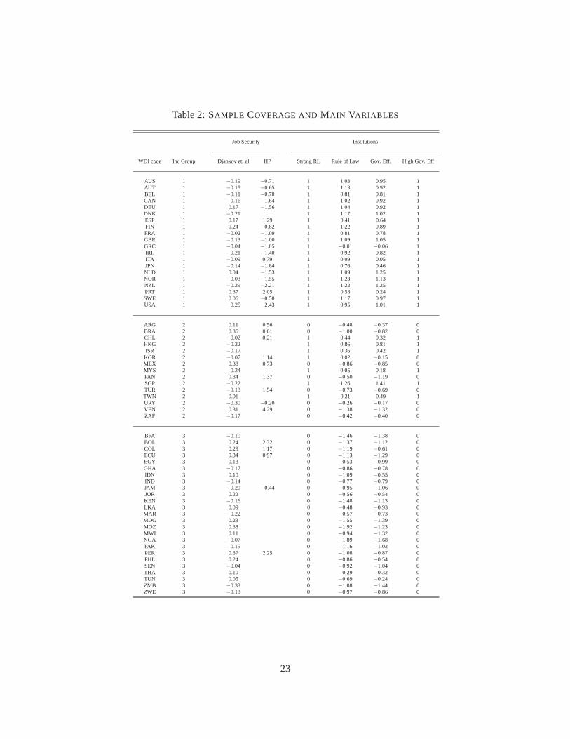
Table 2:SAMPLE COVERAGE AND MAIN VARIABLES

Job Security Institutions

WDI code Inc Group Djankov et. al HP Strong RL Rule of Law Gov. Eff. High Gov. Eff

AUS 1 −0.19 −0.71 1 1.03 0.95 1AUT 1 −0.15 −0.65 1 1.13 0.92 1BEL 1 −0.11 −0.70 1 0.81 0.81 1CAN 1 −0.16 −1.64 1 1.02 0.92 1DEU 1 0.17 −1.56 1 1.04 0.92 1DNK 1 −0.21 1 1.17 1.02 1ESP 1 0.17 1.29 1 0.41 0.64 1FIN 1 0.24 −0.82 1 1.22 0.89 1FRA 1 −0.02 −1.09 1 0.81 0.78 1GBR 1 −0.13 −1.00 1 1.09 1.05 1GRC 1 −0.04 −1.05 1 −0.01 −0.06 1IRL 1 −0.21 −1.40 1 0.92 0.82 1ITA 1 −0.09 0.79 1 0.09 0.05 1JPN 1 −0.14 −1.84 1 0.76 0.46 1NLD 1 0.04 −1.53 1 1.09 1.25 1NOR 1 −0.03 −1.55 1 1.23 1.13 1NZL 1 −0.29 −2.21 1 1.22 1.25 1PRT 1 0.37 2.05 1 0.53 0.24 1SWE 1 0.06 −0.50 1 1.17 0.97 1USA 1 −0.25 −2.43 1 0.95 1.01 1

ARG 2 0.11 0.56 0 −0.48 −0.37 0BRA 2 0.36 0.61 0 −1.00 −0.82 0CHL 2 −0.02 0.21 1 0.44 0.32 1HKG 2 −0.32 1 0.86 0.81 1ISR 2 −0.17 1 0.36 0.42 1KOR 2 −0.07 1.14 1 0.02 −0.15 0MEX 2 0.38 0.73 0 −0.86 −0.85 0MYS 2 −0.24 1 0.05 0.18 1PAN 2 0.34 1.37 0 −0.50 −1.19 0SGP 2 −0.22 1 1.26 1.41 1TUR 2 −0.13 1.54 0 −0.73 −0.69 0TWN 2 0.01 1 0.21 0.49 1URY 2 −0.30 −0.20 0 −0.26 −0.17 0VEN 2 0.31 4.29 0 −1.38 −1.32 0ZAF 2 −0.17 0 −0.42 −0.40 0

BFA 3 −0.10 0 −1.46 −1.38 0BOL 3 0.24 2.32 0 −1.37 −1.12 0COL 3 0.29 1.17 0 −1.19 −0.61 0ECU 3 0.34 0.97 0 −1.13 −1.29 0EGY 3 0.13 0 −0.53 −0.99 0GHA 3 −0.17 0 −0.86 −0.78 0IDN 3 0.10 0 −1.09 −0.55 0IND 3 −0.14 0 −0.77 −0.79 0JAM 3 −0.20 −0.44 0 −0.95 −1.06 0JOR 3 0.22 0 −0.56 −0.54 0KEN 3 −0.16 0 −1.48 −1.13 0LKA 3 0.09 0 −0.48 −0.93 0MAR 3 −0.22 0 −0.57 −0.73 0MDG 3 0.23 0 −1.55 −1.39 0MOZ 3 0.38 0 −1.92 −1.23 0MWI 3 0.11 0 −0.94 −1.32 0NGA 3 −0.07 0 −1.89 −1.68 0PAK 3 −0.15 0 −1.16 −1.02 0PER 3 0.37 2.25 0 −1.08 −0.87 0PHL 3 0.24 0 −0.86 −0.54 0SEN 3 −0.04 0 −0.92 −1.04 0THA 3 0.10 0 −0.29 −0.32 0TUN 3 0.05 0 −0.69 −0.24 0ZMB 3 −0.33 0 −1.08 −1.44 0ZWE 3 −0.13 0 −0.97 −0.86 0

23

Table 3:BASELINE SAMPLE STATISTICS∗

Employment Growth (Yearly Avge.): 1980-2000Inc. Group Obs. Mean SD Min Max

1 8,607 −0.01 0.06 −0.24 0.262 6,063 0.00 0.11 −0.43 0.423 7,063 0.02 0.16 −0.78 0.96

Total 21,733 0.00 0.11 −0.78 0.96

Job Securityfrom Djankov et al. (2003): JSInc. Group Countries Mean SD Min Max

1 20 −0.05 0.18 −0.29 0.372 15 −0.01 0.25 −0.32 0.383 25 0.05 0.21 −0.33 0.38

Total 60 0.00 0.21 −0.33 0.38

Job Securityfrom Heckman and Pages (2001): HPInc. Group Countries Mean SD Min Max

1 19 −0.87 1.15 −2.43 2.052 9 1.14 1.30 −0.20 4.293 5 1.26 1.13 −0.44 2.32

Total 33 0.00 1.54 −2.43 4.29

Rule of Law fromKaufmann et al. (1999): RLInc. Group Countries Mean SD Min Max

1 20 0.88 0.37 −0.01 1.232 15 −0.16 0.72 −1.38 1.263 25 −1.03 0.42 −1.92 −0.29

Total 60 −0.18 0.96 −1.92 1.26

Government Effectivenessfrom Kaufmann et al. (1999): GEInc. Group Countries Mean SD Min Max

1 20 0.80 0.37 −0.06 1.252 15 −0.16 0.76 −1.32 1.413 25 −0.95 0.36 −1.68 −0.24

Total 60 −0.17 0.90 −1.68 1.41

Correlation Country MeansJS HP RL GE

JS 1.00HP 0.66 1.00RL −0.36 −0.77 1.00GE −0.35 −0.77 0.97 1.00

∗Income groups are: 1=High Income OECD, 2=High In-come Non OECD and Upper Middle Income, 3=Lower Mid-dle Income and Low Income.

24

Table 4:ESTIMATION RESULTS

(1) (2) (3) (4) (5) (6) (7) (8)Change in Log-Employment

Gap (λ1) 0.600 0.603 0.607 0.611(0.009)∗∗∗ (0.008)∗∗∗ (0.012)∗∗∗ (0.012)∗∗∗

Gap×JS (λ2): −0.080 −0.015 −0.025 −0.126 −0.027 −0.038(0.037)∗∗ (0.051) (0.051) (0.041)∗∗∗ (0.052) (0.051)

Gap×JS×DSRL (λ3) −0.514 −0.314(0.068)∗∗∗ (0.070)∗∗∗

Gap×JS×DHGE (λ3) −0.515 −0.326(0.068)∗∗∗ (0.071)∗∗∗

Gap×HP (λ2) −0.022(0.007)∗∗∗

Controls

Gap×Dummy High RL −0.076 0.086(0.015)∗∗∗ (0.023)∗∗∗

Gap×Dummy High GE −0.091 0.045(0.015)∗∗∗ (0.023)∗

Observations 21,733 21,733 21,733 21,733 21,733 21,733 21,733 12,012R-squared 0.60 0.60 0.60 0.60 0.61 0.61 0.61 0.62Gap-Income Interaction No No No No Yes Yes Yes YesGap-Sector Interaction No No No No Yes Yes Yes Yes

* significant at 10%; ** significant at 5%; *** significant at 1%. Robust standard errors in parentheses. JS and HP stand for the Djankov et al.

(2003) and Heckman and Pages (2000) job security measures, respectively. DSRL and DHGE stand for strong Rule of Law and high Government

Efficiency dummies (in both cases the threshold is given by Greece, see the main text), respectively, using the Kaufmann et al. (1999) indices. Each

regression has country-year fixed effects. Gaps are estimated using a constantφ = 0.40. Sample excludes the upper and lower 1% of∆e and of the

estimated values of Gap.

25

Tabl

e5:

RO

BU

ST

NE

SS

OFM

AIN

RE

SU

LTS

TO

ALT

ER

NA

TIV

ES

PE

CIF

ICA

TIO

NS

φva

ries

acro

ssφ

varie

sac

ross

φ=

0.40

inco

me

grou

psjo

bse

curit

ygr

oups

θ=

ma(

3)θ

=m

a(4)

dw(1

)(2

)(3

)(4

)(5

)(6

)(7

)(8

)(9

)(1

0)

Cha

nge

inLo

g-E

mpl

oym

ent

Gap

0.56

80.

574

0.56

40.

529

0.59

0(0

.009

)∗∗∗

(0.0

08)∗∗∗

(0.0

08)∗∗∗

(0.0

08)∗∗∗

(0.0

09)∗∗∗

Gap×J

S−0

.094

−0.0

13−0

.027

0.04

6−0

.069

−0.0

08−0

.009

0.06

3−0

.108

−0.1

35(0

.038

)∗∗∗

(0.0

51)

(0.0

37)

(0.0

51)

(0.0

37)

∗(0

.050

)(0

.036

)(0

.050

)(0

.038

)∗∗∗

(0.0

50)∗∗∗

Gap×D

SR

L−0

.051

−0.0

71−0

.085

−0.0

82−0

.106

(0.0

15)∗∗∗

(0.0

15)∗∗∗

(0.0

15)∗∗∗

(0.0

15)∗∗∗

(0.0

16)∗∗∗

Gap×J

S×D

SR

L−0

.501

−0.5

32−0

.515

−0.5

38−0

.258

(0.0

69)∗∗∗

(0.0

69)∗∗∗

(0.0

68)∗∗∗

(0.0

68)∗∗∗

(0.0

71)∗∗∗

Obs

erva

tions

21,7

3321

,732

20,9

0220

,219

20,4

39R

-squ

ared

0.58

0.58

0.58

0.58

0.59

0.59

0.58

0.58

0.60

0.60

Gap

-Sec

tor

Int.

No

Yes

No

Yes

No

Yes

No

Yes

No

Yes

*si

gnifi

cant

at10

%;*

*si

gnifi

cant

at5%

;***

sign

ifica

ntat

1%.

Rob

usts

tand

ard

erro

rsin

pare

nthe

ses.

JSst

ands

for

the

Dja

nkov

etal

.(20

03)

job

secu

rity

mea

sure

.D

SR

Lst

ands

for

high

(abo

veG

reec

e,se

em

ain

text

)R

ule

ofLa

wus

ing

the

Kau

fman

net

al.(

1999

)m

easu

re.

Col

umns

(1),

(2),

(3)

and

(4)

use

valu

esofφ

estim

ated

inTa

ble

1.S

ampl

esex

clud

eth

eup

per

and

low

er1%

of∆e

and

ofth

ees

timat

edva

lues

ofG

ap.

26

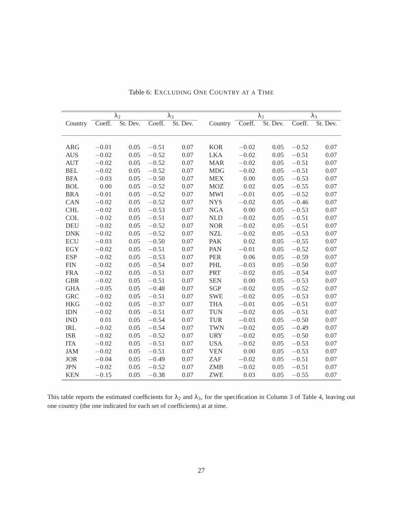
Table 6:EXCLUDING ONE COUNTRY AT A TIME

λ2 λ3 λ2 λ3

Country Coeff. St. Dev. Coeff. St. Dev. Country Coeff. St. Dev. Coeff. St. Dev.

ARG −0.01 0.05 −0.51 0.07 KOR −0.02 0.05 −0.52 0.07AUS −0.02 0.05 −0.52 0.07 LKA −0.02 0.05 −0.51 0.07AUT −0.02 0.05 −0.52 0.07 MAR −0.02 0.05 −0.51 0.07BEL −0.02 0.05 −0.52 0.07 MDG −0.02 0.05 −0.51 0.07BFA −0.03 0.05 −0.50 0.07 MEX 0.00 0.05 −0.53 0.07BOL 0.00 0.05 −0.52 0.07 MOZ 0.02 0.05 −0.55 0.07BRA −0.01 0.05 −0.52 0.07 MWI −0.01 0.05 −0.52 0.07CAN −0.02 0.05 −0.52 0.07 NYS −0.02 0.05 −0.46 0.07CHL −0.02 0.05 −0.53 0.07 NGA 0.00 0.05 −0.53 0.07COL −0.02 0.05 −0.51 0.07 NLD −0.02 0.05 −0.51 0.07DEU −0.02 0.05 −0.52 0.07 NOR −0.02 0.05 −0.51 0.07DNK −0.02 0.05 −0.52 0.07 NZL −0.02 0.05 −0.53 0.07ECU −0.03 0.05 −0.50 0.07 PAK 0.02 0.05 −0.55 0.07EGY −0.02 0.05 −0.51 0.07 PAN −0.01 0.05 −0.52 0.07ESP −0.02 0.05 −0.53 0.07 PER 0.06 0.05 −0.59 0.07FIN −0.02 0.05 −0.54 0.07 PHL −0.03 0.05 −0.50 0.07FRA −0.02 0.05 −0.51 0.07 PRT −0.02 0.05 −0.54 0.07GBR −0.02 0.05 −0.51 0.07 SEN 0.00 0.05 −0.53 0.07GHA −0.05 0.05 −0.48 0.07 SGP −0.02 0.05 −0.52 0.07GRC −0.02 0.05 −0.51 0.07 SWE −0.02 0.05 −0.53 0.07HKG −0.02 0.05 −0.37 0.07 THA −0.01 0.05 −0.51 0.07IDN −0.02 0.05 −0.51 0.07 TUN −0.02 0.05 −0.51 0.07IND 0.01 0.05 −0.54 0.07 TUR −0.03 0.05 −0.50 0.07IRL −0.02 0.05 −0.54 0.07 TWN −0.02 0.05 −0.49 0.07ISR −0.02 0.05 −0.52 0.07 URY −0.02 0.05 −0.50 0.07ITA −0.02 0.05 −0.51 0.07 USA −0.02 0.05 −0.53 0.07JAM −0.02 0.05 −0.51 0.07 VEN 0.00 0.05 −0.53 0.07JOR −0.04 0.05 −0.49 0.07 ZAF −0.02 0.05 −0.51 0.07JPN −0.02 0.05 −0.52 0.07 ZMB −0.02 0.05 −0.51 0.07KEN −0.15 0.05 −0.38 0.07 ZWE 0.03 0.05 −0.55 0.07

This table reports the estimated coefficients forλ2 andλ3, for the specification in Column 3 of Table 4, leaving outone country (the one indicated for each set of coefficients) at at time.

27

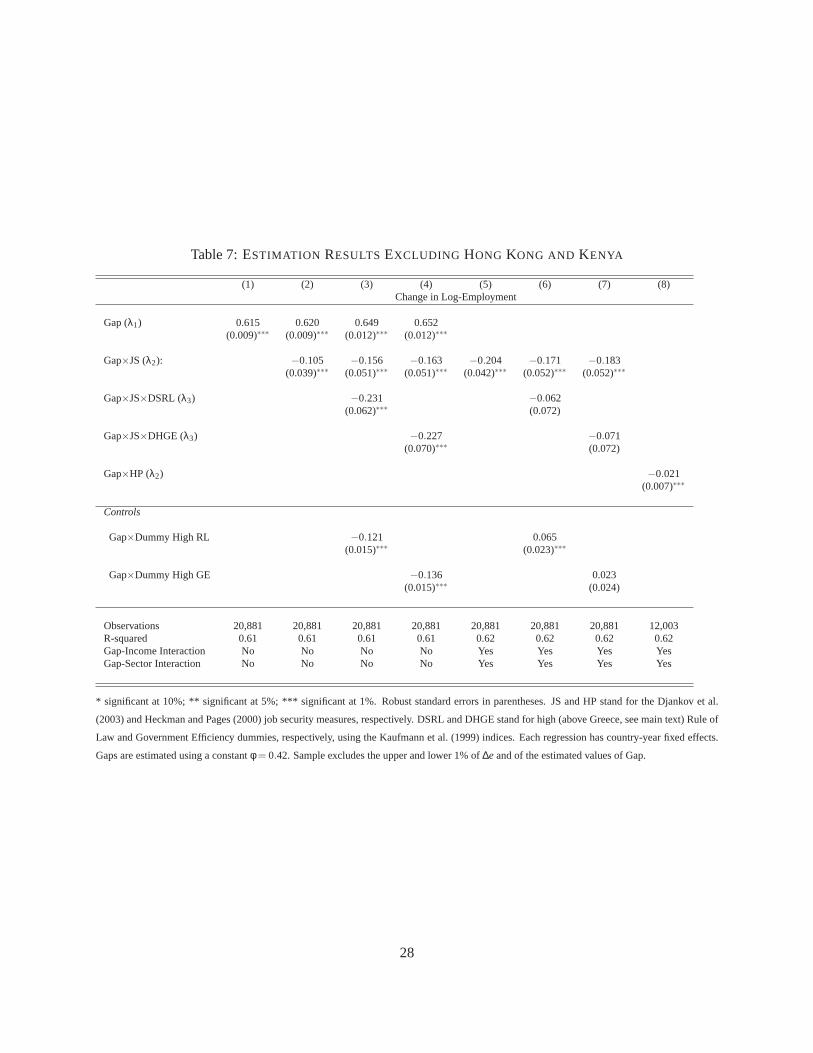
Table 7:ESTIMATION RESULTSEXCLUDING HONG KONG AND KENYA

(1) (2) (3) (4) (5) (6) (7) (8)Change in Log-Employment

Gap (λ1) 0.615 0.620 0.649 0.652(0.009)∗∗∗ (0.009)∗∗∗ (0.012)∗∗∗ (0.012)∗∗∗

Gap×JS (λ2): −0.105 −0.156 −0.163 −0.204 −0.171 −0.183(0.039)∗∗∗ (0.051)∗∗∗ (0.051)∗∗∗ (0.042)∗∗∗ (0.052)∗∗∗ (0.052)∗∗∗

Gap×JS×DSRL (λ3) −0.231 −0.062(0.062)∗∗∗ (0.072)

Gap×JS×DHGE (λ3) −0.227 −0.071(0.070)∗∗∗ (0.072)

Gap×HP (λ2) −0.021(0.007)∗∗∗

Controls

Gap×Dummy High RL −0.121 0.065(0.015)∗∗∗ (0.023)∗∗∗

Gap×Dummy High GE −0.136 0.023(0.015)∗∗∗ (0.024)

Observations 20,881 20,881 20,881 20,881 20,881 20,881 20,881 12,003R-squared 0.61 0.61 0.61 0.61 0.62 0.62 0.62 0.62Gap-Income Interaction No No No No Yes Yes Yes YesGap-Sector Interaction No No No No Yes Yes Yes Yes

* significant at 10%; ** significant at 5%; *** significant at 1%. Robust standard errors in parentheses. JS and HP stand for the Djankov et al.

(2003) and Heckman and Pages (2000) job security measures, respectively. DSRL and DHGE stand for high (above Greece, see main text) Rule of

Law and Government Efficiency dummies, respectively, using the Kaufmann et al. (1999) indices. Each regression has country-year fixed effects.

Gaps are estimated using a constantφ = 0.42. Sample excludes the upper and lower 1% of∆eand of the estimated values of Gap.

28

Table 8:IV ESTIMATION

Average speed of adjustment

Estimation Method Point Estimate Robust Standard Error

Baseline Model (Column 1 in Table 4 0.600 0.009

Gap instrumented with wage data 0.570 0.065

Standard dynamic panel formulation 0.543 0.078

See section 3.2.3 for details.

29

Table 9:ESTIMATING COUNTRY-SPECIFICSPEEDS OFADJUSTMENT

Country λc,1 St. Dev. λc,2 St. Dev. Country λc,1 St. Dev. λc,2 St. Dev.

ARG 0.380 0.060 0.364 0.071 KOR 0.719 0.028 0.696 0.052AUS 0.558 0.048 0.537 0.063 LKA 0.744 0.041 0.729 0.056AUT 0.521 0.040 0.504 0.056 MAR 0.572 0.060 0.569 0.071BEL 0.160 0.046 0.158 0.062 MDG 0.688 0.067 0.666 0.075BFA 0.327 0.066 0.309 0.076 MEX 0.467 0.042 0.451 0.058BOL 0.562 0.049 0.545 0.064 MOZ 0.414 0.111 0.370 0.122BRA 0.385 0.067 0.346 0.078 MWI 0.499 0.095 0.437 0.094CAN 0.565 0.038 0.547 0.055 NYS 0.750 0.032 0.723 0.053CHL 0.631 0.045 0.618 0.061 NGA 0.782 0.094 0.754 0.102COL 0.624 0.030 0.591 0.052 NLD 0.467 0.060 0.414 0.073DEU 0.463 0.048 0.458 0.062 NOR 0.472 0.037 0.468 0.054DNK 0.500 0.058 0.488 0.070 NZL 0.483 0.065 0.443 0.076ECU 0.645 0.044 0.624 0.059 PAK 0.771 0.054 0.740 0.069EGY 0.694 0.052 0.671 0.065 PAN 0.575 0.049 0.561 0.064ESP 0.488 0.033 0.469 0.052 PER 0.379 0.038 0.376 0.056FIN 0.445 0.032 0.428 0.051 PHL 0.664 0.036 0.652 0.055FRA 0.292 0.032 0.278 0.052 PRT 0.369 0.029 0.362 0.050GBR 0.577 0.037 0.565 0.054 SEN 0.716 0.080 0.707 0.090GHA 0.502 0.064 0.498 0.075 SGP 0.631 0.039 0.605 0.057GRC 0.552 0.032 0.536 0.052 SWE 0.578 0.037 0.555 0.054HKG 0.837 0.029 0.821 0.050 THA 0.490 0.143 0.450 0.142IDN 0.676 0.046 0.645 0.061 TUN 0.633 0.099 0.605 0.099IND 0.746 0.051 0.736 0.067 TUR 0.506 0.031 0.475 0.051IRL 0.516 0.031 0.488 0.051 TWN 0.406 0.037 0.379 0.056ISR 0.606 0.040 0.592 0.057 URY 0.584 0.034 0.575 0.053ITA 0.364 0.047 0.341 0.062 USA 0.544 0.040 0.542 0.056JAM 0.563 0.411 0.510 0.364 VEN 0.519 0.037 0.515 0.056JOR 0.697 0.041 0.681 0.057 ZAF 0.581 0.044 0.548 0.059JPN 0.470 0.035 0.463 0.054 ZMB 0.482 0.095 0.457 0.106KEN 0.224 0.038 0.201 0.055 ZWE 0.774 0.051 0.749 0.064

1st quintile 0.346 0.3252nd quintile 0.482 0.4573rd quintile 0.546 0.5274th quintile 0.619 0.6005th quintile 0.743 0.723

This table reports estimated coefficients forλ at the country level. A common value ofφ = 0.40 is used throughout.λc,2 includes sectoral controls, whileλc,1 does not.

30

Table 10:PRODUCTIVITY GROWTH AND SPEED OFADJUSTMENT I

Change inλc-Quintile Change in Annual Growth Rate

1st to 2nd 0.88%

2nd to 3rd 0.29%

3rd to 4th 0.23%

4th to 5th 0.28%

1st to 5th 1.68%

Reported: change in annual growth rates associated with moving from the average adjustment speed of one quintile to the

next. Quintiles forλc from Table 9, column with sectoral controls. Calculation based on model described in Section 4 (see

equation (19)). Parameter values:γ = 5/6), gY,1 = 0.007, σ = 0.27 α = 2/3, andδ = 0.06.

31

Table 11:PRODUCTIVITY GROWTH AND SPEED OFADJUSTMENT II

(1) (2) (3) (4) (5) (6)Annual Average Change in TFP 1980-1990

Speed of adjustment: 0.040 0.031 0.053 0.026 0.026 0.046(0.018)∗∗ (0.019)∗ (0.018)∗∗∗ (0.019) (0.019) (0.019)∗∗

Constant: −0.016 −0.013 −0.016 −0.012 −0.012 −0.014(0.010) (0.010) (0.009)∗ (0.011) (0.010) (0.009)

Observations 42 42 42 42 42 42R-squared 0.108 0.066 0.294 0.043 0.041 0.230Income Fixed Effects No No Yes No No YesEstimation via WLS WLS WLS OLS OLS OLS

* significant at 10%; ** significant at 5%; *** significant at 1%. Robust standard errors in parentheses. Sample-

size determined by availability of TFP data. TFP growth at the country level calculated following Mankiw (1995):

TFP growth = Per-capita GDP growth - 0.3 Per-capita capital growth - 0.5 Avge. Schooling growth. The data

comes from World Penn Tables 5.6 and Barro and Lee (1996). WLS refers to weighted least squares, with

weights inversely proportional to the standard deviation of estimatedλc’s. OLS refers to ordinary least squares.

32