Embed Size (px)
Citation preview
Semantic Web tbd (2016) 1–39 1IOS Press
Effective and Efficient Semantic TableInterpretation using TableMiner+
Editor(s): Pascal Hitzler, Wright State University, USA; Isabel Cruz, University of Illinois at Chicago, USASolicited review(s): Michael Granitzer, Universität Passau, Germany; Mike Cafarella, University of Michigan, USA; Venkat Raghavan Ganesh,University of Illinois at Chicago, USA
Ziqi ZhangSchool of Science and Technology, Nottingham Trent University, 50 Shakespeare Street, Nottingham, NG1 4FQ(This work was carried out while the author was a member of the Department of Computer Science, University ofSheffield)E-mail: [email protected]
Abstract. This article introduces TableMiner+, a Semantic Table Interpretation method that annotates Web tables in a botheffective and efficient way. Built on our previous work TableMiner, the extended version advances state-of-the-art in several ways.First, it improves annotation accuracy by making innovative use of various types of contextual information both inside and outsidetables as features for inference. Second, it reduces computational overheads by adopting an incremental, bootstrapping approachthat starts by creating preliminary and partial annotations of a table using ‘sample’ data in the table, then using the outcome as‘seed’ to guide interpretation of remaining contents. This is then followed by a message passing process that iteratively refinesresults on the entire table to create the final optimal annotations. Third, it is able to handle all annotation tasks of SemanticTable Interpretation (e.g., annotating a column, or entity cells) while state-of-the-art methods are limited in different ways.We also compile the largest dataset known to date and extensively evaluate TableMiner+ against four baselines and two re-implemented (near-identical, as adaptations are needed due to the use of different knowledge bases) state-of-the-art methods.TableMiner+ consistently outperforms all models under all experimental settings. On the two most diverse datasets coveringmultiple domains and various table schemata, it achieves improvement in F1 by between 1 and 42 percentage points dependingon specific annotation tasks. It also significantly reduces computational overheads in terms of wall-clock time when comparedagainst classic methods that ‘exhaustively’ process the entire table content to build features for inference. As a concrete example,compared against a method based on joint inference implemented with parallel computation, the non-parallel implementationof TableMiner+ achieves significant improvement in learning accuracy and almost orders of magnitude of savings in wall-clocktime.
Keywords: Web table, Named Entity Recognition, Named Entity Disambiguation, Relation Extraction, Linked Data, SemanticTable Interpretation, table annotation
1. Introduction
Recovering semantics from tables is a crucial taskin realizing the vision of the Semantic Web. On theone hand, the amount of high-quality tables containinguseful relational data is growing rapidly to hundreds ofmillions [3,4]. On the other hand, search engines typ-ically ignore underlying semantics of such structuresat indexing, hence performing poorly on tabular data
[21,24]. Research directed to this particular problem isSemantic Table Interpretation [14,15,21,25,7,23,35,36,2,24,26], which deals with three types of annotationtasks in tables. Starting with the input of a well-formedrelational table (e.g., Figure 1), and reference sets ofconcepts (or classes, types), named entities (or simply‘entities’) and relations, semantic table interpretationaims to: (1) link entity mentions in content cells (orsimply ‘cells’) to the reference entities (disambigua-
1570-0844/16/$27.50 © 2016 – IOS Press and the authors. All rights reserved

2 Z. Zhang / Effective and Efficient Semantic Table Interpretation using TableMiner+
tion); (2) annotate columns with semantic concepts ifthey contain entity mentions (NE-columns), or prop-erties of concepts if they contain data literals (literal-columns); and (3) identify the semantic relations be-tween columns. The annotations created can enable se-mantic indexing and search of the data and used to cre-ate Linked Open Data (LOD).
Although classic Natural Language Processing (NLP)and Information Extraction (IE) techniques addresssimilar research problems [45,10,5,28], they are tai-lored for well-formed sentences in unstructured texts,and are unlikely to succeed on tabular data [21,24].Typical Semantic Table Interpretation methods makeextensive use of structured knowledge bases, whichcontain candidate concepts and entities, each definedwith rich lexical and semantic information and linkedby relations. The general workflow involves: (1) re-trieving candidates corresponding to table components(e.g., concepts given a column header, or entities giventhe text of a cell) from the knowledge base, (2) repre-sent candidates using features extracted from both theknowledge base and tables to model semantic inter-dependence between table components and candidates(e.g., the header text of a column and the name of acandidate concept), and between various table compo-nents (e.g., a column should be annotated by a con-cept that is shared by all entities in the cells from thecolumn), and (3) applying inference to choose the bestcandidates.
This work addresses several limitations of state-of-the-art on three dimensions: effectiveness, efficiency,and completeness.
Effectiveness - Semantic Table Interpretation meth-ods so far have primarily exploited features derivedfrom two sources: the knowledge bases, and table com-ponents such as header and row content (to be called‘in-table context’). In this work, we propose to uti-lize the so-called ‘out-table context’, i.e., the textualcontent around and outside tables (e.g., paragraphs,captions), to further improve interpretation accuracy.As an example, the first column in the table shownin Figure 1 (to be called the ‘example table’) hasa header ‘Title’, which is highly ambiguous and ar-guably irrelevant to the concept we should use to an-notate the column. However, on the containing web-page, the word ‘film’ is repeated 17 times. This is astrong indicator for us to select a suitable concept forthe column. A particular type of out-table context weutilize is the semantic markups inserted within web-pages by data publishers such as RDFa/Microdata an-notations. These markups are growing rapidly as major
search engines use them to enable semantic indexingand search. When available, they provide high-quality,important information about the webpages and tablesthey contain.
We show empirically that we can derive useful fea-tures from out-table context to improve annotation ac-curacy. Such out-table features are highly generic andgenerally available. While on the contrary, many exist-ing methods use knowledge base specific features thatare impossible to generalize, or suffer substantially interms of accuracy when they can be adapted, which weshall show in experiments.
Efficiency - We argue that efficiency is also an im-portant factor to consider in the task of Semantic TableInterpretation, even though it has never been explic-itly addressed before. The major bottleneck is mainlydue to three types of operations: querying the knowl-edge bases, building feature representations for can-didates, and computing similarity between candidates.Both the number of queries and similarity computationcan grow quadratically with respect to the size of a ta-ble as often such operations are required for each pairof candidates [21,24,27]. Empirically, Limaye et al.[21] show that the actual inference algorithm only con-sumes less than 1% of total running time. Using a localcopy of the knowledge base only partially addressesthe issue but introduces more problems. First, hostinga local knowledge base requires infrastructural supportand involves set-up and maintenance. As we enter the‘Big-Data’ era, knowledge bases are growing rapidlytowards a colossal structure such as the Google Knowl-edge Graph [33], which constantly integrates increas-ing numbers of heterogeneous sources. Maintaining alocal copy of such a knowledge base is likely to requirean infrastructure that not every organization can afford[29]. Second, local data are not guaranteed to be up-to-date. Third, scaling up to very large amount of inputdata requires efficient algorithms in addition to paral-lelization [32], as the process could be bound by thelarge number of I/O operations. Therefore in our view,a more versatile solution is cutting down the numberof queries and data items to be processed. This reducesI/O operations in both local and remote scenarios, alsoreducing costs associated with making remote calls toWeb service providers.
In this direction, we identify an opportunity to im-prove state-of-the-art in terms of efficiency. To illus-trate, consider the example table that in reality con-tains over 60 rows. To annotate each column, existingmethods would use content from every row in the col-umn. However, from a human reader’s point of view,

Z. Zhang / Effective and Efficient Semantic Table Interpretation using TableMiner+ 3
Fig. 1. An example Wikipedia webpage containing a relational table (Last retrieved on 9 April 2014).
this is unnecessary. Simply reading the eight rows onecan confidently assign a concept to the column to bestdescribe its content. Being able to make such inferencewith limited data would give substantial efficiency ad-vantage to Semantic Table Interpretation algorithms,as it will significantly reduce the number of queriesto the underlying knowledge bases and the number ofcandidates to be considered for inference.
Completeness - Many existing methods only dealwith one or two types of annotation tasks in a table[35,36]. In those that deal with all tasks [21,25,23,24,7], only NE-columns are considered. As shown inFigure 1, tables can contain both NE-columns con-taining entity mentions, and literal-columns contain-ing data values of entities on the corresponding rows.Methods such as Limaye et al. [21] and Mulwad etal. [24] can recognize relations between the first andthird columns, but are unable to identify the relationbetween the first and the second columns. We arguethat a Semantic Table Interpretation method should beable to annotate both NE-columns and literal-columns.
To address these issues, we developed TableMinerpreviously [42] that uses features from both in- andout-table context and annotates NE-columns and cellsin a relational table based on the principle of ‘startsmall, build complete’. That is, (1) create prelimi-nary, likely erroneous annotations based on partial ta-ble content and a simple model assuming limited in-
terdependence between table components; (2) and theniteratively optimize the preliminary annotations by en-forcing interdependence between table components. Inthis work we extend it to build TableMiner+, by adding‘subject column’ [35,36] detection, relation enumera-tion, and improving the iterative optimization process.Concretely, TableMiner+ firstly interprets NE-columns(to be called column interpretation), while couplingcolumn classification and entity disambiguation in amutually recursive process that consists of a LEARN-ING phase and an UPDATE phase. The LEARNINGphase interprets each column independently by firstlylearning to create preliminary column annotations us-ing an automatically determined ‘sample’ from thecolumn, followed by ‘constrained’ entity disambigua-tion of the cells in the column (limiting candidate en-tity space using preliminary column annotations). TheUPDATE phase iteratively optimizes the classificationand disambiguation results in each column based ona notion of ‘domain consensus’ that captures inter-column and inter-task dependence, creating a globaloptimum. For relation enumeration, TableMiner+ de-tects a subject column in a table and infers its relationswith other columns (both NE- and literal-columns) inthe table.
TableMiner+ is evaluated on four datasets contain-ing over 15,000 tables, against four baselines and two
4 Z. Zhang / Effective and Efficient Semantic Table Interpretation using TableMiner+
re-implemented near-identical1 state-of-the-art meth-ods. It consistently obtains the best performance onall datasets. On the two most diverse datasets coveringmultiple domains and various table schemata, it ob-tains an improvement of about 1-18 percentage pointsin disambiguation, 6-42 in classification, and 4-16 inrelation enumeration. It is also very efficient, con-tributing up to 66% reduction in terms of the amountof candidates to be processed and up to 29% savingsin wall-clock time compared against exhaustive base-line methods. Even in the setting where a local copyof the knowledge base is used, TableMiner+ deliversalmost orders of magnitude savings in wall-clock timecompared against one re-implemented state-of-the-artmethod.
The remainder of this paper is organized as follows.Section 2 defines terms and concepts used in the rel-evant domain. Section 3 discusses related work. Sec-tions 4 to 9 introduce TableMiner+ in detail. Sections10 and 11 describe experiment settings and discuss re-sults, followed by conclusion in Section 12.
2. Terms and concepts
A relational table contains regular rows and columnsresembling tables in traditional databases. In practice,Web tables containing complex structures constitute asmall population and have not been the focus of re-search. In theory, complex tables can be interpretedby adding a pre-process that parse complex structuresusing methods such as Zanibbi et al. [39]
Relational tables may or may not contain a headerrow, which is typically the first row in a table. They of-ten contain a subject column that usually (but not nec-essarily) corresponds to the ‘primary key’ columns in adatabase table [35,36]. This contains the set of entitiesthe table is about (subject entities, e.g., column ‘Title’in Figure 1 contains a list of films the table is about),while other columns contain either entities forming bi-nary relationships with subject entities, or literals de-scribing attributes of subject entities.
A knowledge base defines a set of concepts (ortypes, classes), their object instances or entities, liter-als representing concrete data values, and semantic re-lations that define possible associations between enti-ties (hence also between concepts they belong to), or
1Despite our best effort, identical replication of existing systemsand experiments has been not possible due to many reasons, see Ap-pendix D.
between an entity and a literal, in which case the rela-tion is usually called a property of the entity (hencea property of its concept) and the literal as the prop-erty value. In the generic form, a knowledge base is aliked data set containing a set of triples, statements,or facts, each composed of a subject, predicate and ob-ject. The subject could be a concept or entity, the ob-ject could be a concept, entity, or literal, and the predi-cate could be a relation or property. A knowledge basecan be a populated ontology, such as the YAGO2 andDBpedia3 datasets, in which case a concept hierarchyis defined. However this is not always true as someknowledge bases do not define strict ontology but looseconcept networks, such as Freebase4.
The task of Semantic Table Interpretation addressesthree annotation tasks. Named Entity Disambiguationassociates each cell in NE-columns with one canon-ical entity; column classification annotates each NE-column with one concept, or in the case of literal-columns, associates the column to one property of theconcept assigned to the subject column of the table;Relation Extraction (or enumeration) identifies binaryrelations between NE-columns, or in the case of oneNE-column and a literal-column and given that theNE-column is annotated by a specific concept, identi-fies a property of that concept that could explain thedata literals. The candidate entities, concepts and rela-tions are drawn from the knowledge base.
Using the example table and Freebase as example,the first column can be considered a reasonable subjectcolumn and should be annotated by the Freebase type‘Film’ (URI ‘fb5:/film/film’). ‘A Difficult Life’ in thefirst column should be annotated by ‘fb:/m/02qlhz2’that denotes a movie directed by ‘Dino Risi’ (in thethird column, ‘fb:/m/0j_nhj’). The relation between thefirst and third column should be annotated as ‘Directedby’ (‘fb:/film/film/directed_by’). And the relation be-tween the first and second column (which is a literal-column) should be the property of ‘Film’: ‘initial re-lease date’ (‘fb:/film/film/initial_release_date’), whichwe also use to annotate the second column.
2http://www.mpi-inf.mpg.de/yago-naga/yago/3http://wiki.dbpedia.org/Ontology4http://www.freebase.com5fb:http://www.freebase.com

Z. Zhang / Effective and Efficient Semantic Table Interpretation using TableMiner+ 5
3. Related work
3.1. Legacy tabular data to linked data
Research on converting tabular data in legacy datasources to linked data format has made solid contri-bution toward the rapid growth of the LOD cloud inthe past decade [12,19,30,6]. The key difference fromthe task of Semantic Table Interpretation is that thefocus is on data generation rather than interpretation,since the goal is to pragmatically convert tabular datafrom databases, spreadsheets, and similar data struc-tures into RDF. Typical methods require manually (orpartially automated) mapping the two data structures(input and output RDF), and they do not link data toexisting concepts, entities and relations from the LODcloud. As a result, the implicit semantics of the dataremain uncovered.
3.2. General NLP and IE
Some may argue to use the general purpose NLP/IEmethods for Semantic Table Interpretation, due to theirhighly similar objectives. This is infeasible for a num-ber of reasons. First, state-of-the-art methods [31,17]are typically tailored to unstructured text content thatis different from tabular data. The interdependenceamong the table components cannot be easily modeledin such methods [22]. Second and particularly for thetasks of Named Entity Classification and Relation Ex-traction, classic methods require each target semanticlabel (i.e., concept or relation) to be pre-defined andlearning requires training or seed data [28,40]. In Se-mantic Table Interpretation however, due to the largedegree of variations in table schemata (e.g., Limaye etal. [21] use a dataset of over 6,000 randomly crawledWeb tables of which no information about the tableschemata is known a priori), defining a comprehen-sive set of semantic concepts and relations and sub-sequently creating necessary training or seed data areinfeasible.
A related IE task tailored to structured data is wrap-per induction [18,9], which automatically learns wrap-pers that can extract information from regular, recur-rent structures (e.g., product attributes from Amazonwebpages). In the context of relational tables, wrap-per induction methods can be adapted to annotate tablecolumns that describe entity attributes. However, theyalso require training data and the table schemata to beknown a priori.
3.3. Table extension and augmentation
Table extension and augmentation aims at gather-ing relational tables that contain the same entities butcover complementary attributes of the entities, and in-tegrate these tables by joining them on the same en-tities. For example, Yakout et al. [38] propose Info-Gather for populating a table of entities with their at-tributes by harvesting related tables on the Web. Theusers need to either provide the desired attribute namesof the entities, or example values of their attributes.The system can also discover the set of attributes forsimilar entities. Bhagavatula et al. [1] introduce Wik-iTables, which given a query table and a collection ofother tables, identifies columns from other tables thatwould make relevant additions to the query table. Theyfirst identify a reference column (e.g., country namesin a table of country population) in the query table touse for joining, then find a different table (e.g. a list ofcountries by GDP) with a column similar to the refer-ence column, and perform a left outer join to augmentthe query table with an automatically selected columnfrom the new table (e.g., the GDP amounts). Lehm-berg et al. [20] create the Mannheim Search Joins En-gine with the same goal as WikiTables but focus onhandling tens of millions of tables from heterogeneoussources.
The key difference between these systems and thetask of Semantic Table Interpretation is that they focuson integration rather than interpretation. The data col-lected are not linked to knowledge bases and ambigu-ity still remains.
3.4. Semantic Table Interpretation
Hignette et al. [14,15] and Buche et al. [2] pro-pose methods to identify concepts represented by ta-ble columns and detect relations present in tables in adomain-specific context. An NE-column is annotatedbased on two factors: similarity between the headertext of the column and the name of a candidate con-cept; plus the similarities calculated for each cell in thecolumn and each term in the hierarchical paths con-taining the candidate concept. For relations, they onlydetect the presence of semantic relations in the tablewithout specifying the columns that form binary rela-tions.
Venetis et al. [35] annotate table columns and iden-tify relations between the subject column and othercolumns using types and relations from a database con-structed by mining the Web using lexico-syntactic pat-

6 Z. Zhang / Effective and Efficient Semantic Table Interpretation using TableMiner+
terns such as the Hearst patterns [13]. The databasecontains co-occurrence statistics about the subject andobject of triples, such as the number of times theword ‘cat’ and ‘animal’ extracted by the pattern <?, suchas, ? > representing the is-a relation betweenconcept and instances. A maximum likelihood infer-ence model predicts the best type for a column to be theone maximizing the probability of seeing all the val-ues in the column given that type for the column. Suchprobability is computed based on the co-occurrencestatistics gathered in the database. Relation interpreta-tion follows the same principle.
Likewise, Wang et al. [36] argue that tables describea single entity type (concept) and its attributes andtherefore, consist of an entity column (subject column)and multiple attribute columns. The goal is to firstlyidentify the entity column in the table, then associatea concept from the Probase knowledge base [37] thatbest describes the table schema. Essentially this allowsannotating the subject NE-column and literal-columnsusing properties of the concept, also identifying rela-tions between the subject column and other columns.Probase is a probabilistic database built in the similarway as that in Venetis et al. [35] and contains an in-verted index that supports searching and ranking can-didate concepts given a list of terms describing pos-sible concept properties, or names describing possi-ble instances. The method heavily depends on thesefeatures and the probability statistics gathered in thedatabase.
Muñoz et al. [26] extract RDF triples for relationaltables from Wikipedia articles. The cells in the tablesmust have internal links to other Wikipedia articles.These are firstly mapped to DBpedia named entitiesbased on the internal links, then to derive relations be-tween two entities on the same row and from differ-ent columns, the authors query the DBpedia dataset fortriples in the form of < subject, ?, object >, wheresubject and object are replaced by the two mapped en-tities. Any predicates found in the query result are con-sidered as relations between the two entities. The workis later extended in Muñoz et al. [27] by adding a ma-chine learning process to filter triples that are likely tobe incorrect, exploiting features derived from both theknowledge base and the text content from the targetcells.
Zwicklbauer et al. [46] use a simple majority votemodel for column classification. Each candidate entityin the cells of the column casts a vote to the conceptit belongs to, and the one that receives the most votesis the concept used to annotate the column. They show
that for this very specific task, it is unnecessary to ex-haustively disambiguate each cell in a column. Instead,comparable accuracy can be obtained by using a frac-tion of the cells from the column. However, the samplesize is arbitrarily decided.
Syed et al. [7] deal with all three annotation tasks us-ing DBpedia and Wikitology [34], the latter of whichcontains an index of Wikipedia articles describing en-tities and a classification system that integrates severalvocabularies including the DBpedia ontology, YAGO,WordNet6 and Freebase. The method begins by firstlyannotating each NE-column based on candidate en-tities from every cell in the column. Candidate enti-ties for each cell are retrieved by composing structuredqueries to match the cell text, the row content, and thecolumn header against different fields defined in theWikitology index, such as the title and redirects, thefirst sentence and links from candidate entities’ origi-nal Wikipedia articles. Candidate concepts for the col-umn combines the types associated with each candi-date entity from each cell, and the scores are based onthe number of candidate entities associated with thatconcept and the relevance score of candidate entitiesin the search results returned by Wikitology. The col-umn annotations are then used as input in Named En-tity Disambiguation, which is cast as queries to Wiki-tology with new constraints using the column’s anno-tation. Finally, relations between two NE-columns arederived based on the similar method by Muñoz et al.[26] using DBpedia. This method is later used in Mul-wad et al. [25] and Mulwad et al. [23].
Limaye et al. [21] propose to model table compo-nents and their interdependence using a probabilisticgraphical model. The model consists of two compo-nents: ‘variables’ that model different table compo-nents, and ‘factors’ that are further divided into nodefactors modeling the compatibility between the vari-able and each of its candidate, and edge factors mod-eling the compatibility between the variables believedto be correlated. For example, given an NE-column,the header of the column is a variable that takes val-ues from a set of candidate concepts; and each cell inthe column is a variable that takes values from a set ofcandidate entities. The node factor for the header couldmodel the compatibility between the header text andthe names of each candidate concept; while the edgefactor could model the compatibility between any can-didate concept for the header and any candidate entity
6http://wordnet.princeton.edu/

Z. Zhang / Effective and Efficient Semantic Table Interpretation using TableMiner+ 7
from each cell. The strength of compatibility could bemeasured using methods such as string similarity met-rics [11] and semantic similarity measures [43]. Thenthe task of inference amounts to searching for an as-signment of values to the variables that maximizes thejoint probability. A unique feature of this method isthat it solves the three annotation tasks simultaneously,capturing interdependence between various table com-ponents at inference, while other methods either tackleindividual annotation tasks or tackles each separatelyand sequentially.
Mulwad et al. [24] argue that computing the jointprobability distribution in Limaye’s method is very ex-pensive. Built on the earlier work by Syed et al. [7]and Mulwad et al. [25,23], they propose a light-weightsemantic message passing algorithm that applies infer-ence to the same kind of graphical model. This is sim-ilar to TableMiner+ in the way that the UPDATE phaseof TableMiner+ can be considered as a similar seman-tic message passing process. However, TableMiner+
is fundamentally different since it (1) adds a subjectcolumn detection algorithm; (2) deals with both NE-columns and literal-columns, while Mulwad et al. onlyhandle NE-columns; (3) uses an efficient approachbootstrapped by sampled data from the table whileMulwad et al. build a model that approaches the task inan exhaustive way; (4) defines and uses context aroundtables as features while Mulwad et al. has used knowl-edge base specific features; (5) uses different methodsfor scoring and ranking candidate entities, conceptsand relations; and (6) models interdependence differ-ently which, if transforms to an equivalent graphicalmodel, would result in fewer factor nodes.
3.5. Remark
Existing Semantic Table Interpretation methodshave several limitations. First, they have not consid-ered using features from out-table context, which ishighly generic and generally available. Instead, manyhave used knowledge base specific features that aredifficult or impossible to generalize. For example, theco-occurrence statistics used by Venetis et al. [35]and Wang et al. [36] are unavailable in knowledgebases such as YAGO, DBpedia, and Freebase. Meth-ods such as Limaye et al. [21] and Mulwad et al. [24]use the concept hierarchy in their knowledge bases.However, Freebase does not have a strict concept hier-archy. These methods can become less effective whenadapted to different knowledge bases, as we shall showlater.
Second, no existing methods explicitly address effi-ciency, which we argue as an important factor in Se-mantic Table Interpretation tasks. Current methods arenon-efficient because they typically adopt an exhaus-tive strategy that examines the entire table content,e.g., column classification depends on every cell in thecolumn. This results in quadratic growth of the num-ber of computations and knowledge base queries withrespect to the size of tables, as such operations are usu-ally required for every pair of candidates, e.g., candi-date relation lookup between every pair of entities onthe same row [24,26,27], or similarity computation be-tween every pair of candidate entity and concept in acolumn [21]. This can be redundant as Zwicklbauer etal. [46] have empirically shown that comparable accu-racy can be obtained by using only a fraction of data(i.e., sample) from the column. However, there remainsthe challenge to automatically determine the optimalsample size and elements.
Further, existing methods are incomplete, since theyeither only tackle certain annotation tasks [35,36], oronly deal with NE-columns [21,25,23,24,7].
In an attempt to address some of the above issues,we previously developed a prototype TableMiner [42]that is able to annotate NE-columns and disambiguateentity cells in an incremental, mutually recursive andbootstrapping approach seeded by automatically se-lected sample from a table. And in Zhang [41] we fur-ther explored different methods for selecting the sam-ple and its effect on accuracy. This work joins the twoand largely extends them in a number ways: (1) addinga new algorithm for subject column detection and forrelation enumeration; (2) revising the column classifi-cation and entity disambiguation processes (primarilyin the UPDATE process); (3) performing significantlymore comprehensive experiments to thoroughly evalu-ate the new method; and (4) releasing both the datasetand software to encourage future research.
4. Overview
Figure 2 shows the data flow and processes ofTableMiner+. Given a relational table it firstly detects asubject column (Section 6), which is used by later pro-cesses of column interpretation and relation enumer-ation. Then TableMiner+ performs NE-column inter-pretation, coupling column classification with entitydisambiguation in an incremental, mutually recursive,bootstrapping approach. This starts with a LEARNINGphase (Section 7) that interprets one NE-column at a

8 Z. Zhang / Effective and Efficient Semantic Table Interpretation using TableMiner+
Fig. 2. The overview of TableMiner+. (a) a high-level architecture diagram; (b) detailed architecture with input/output. d - table data. Grey colourindicates annotated table elements. Angle brackets indicates annotations. Inside a table: H - header. E, a, b, x, z - content cells
time independently to create preliminary concept an-notation for an NE-column and entity annotation forthe cells, followed by an UPDATE phase (Section 8)that iteratively revises the annotations by enforcinginterdependence between columns, and between theclassification and disambiguation results.
In the LEARNING phase, for preliminary columnclassification (Section 7.2), TableMiner+ works in anincremental, iterative manner to gather evidence fromeach cell in the column at a time until it reaches astopping criteria (automatically determined), usuallybefore covering all cells in the column. Therefore,TableMiner+ can use only partial content in the columnto perform column classification. We say that it usesa ‘sample’ from the column for the task and each el-ement in the sample is a cell which TableMiner+ hasused as evidence for preliminary column classificationuntil stop. In theory, the size and elements of the sam-
ple can affect the outcome and hence the accuracy ofclassification. For this reason, a sample ranking pro-cess (Section 7.1) precedes preliminary column clas-sification to re-order table rows based on the cells inthe target column with a goal to optimize the sam-ple to obtain the highest accuracy of classification.Next, the preliminary concept annotation for the col-umn is used to constrain entity candidate space in dis-ambiguating cells in the column (preliminary cell dis-ambiguation, Section 7.3). Using a sample for columnclassification and constraining entity candidate spaceallows TableMiner+ to be more efficient than state-of-the-art methods that exhaustively process all contentfrom a column.
The UPDATE phase begins by taking the entity an-notations in all NE-cells to create a ‘domain represen-tation’ (Section 8.1), which is compared against candi-date concepts for each NE-column to revise the prelim-

Z. Zhang / Effective and Efficient Semantic Table Interpretation using TableMiner+ 9
inary column classification results (Section 8.2). If anyNE-column’s annotation changes due to this process,the newly elected concept is then used to revise dis-ambiguation results in that column (Section 8.3). Thisprocess repeats until no changes are required.
Finally relation enumeration (Section 9) discoversbinary relations between the subject column and otherNE-columns; or identifies a property of the conceptused to annotate the subject column to best describedata in the literal-columns. In the latter case, the prop-erty is considered both the annotation for the literal-column, and the relation between the subject columnand the literal-column.
The incremental, iterative process used by prelimi-nary column classification is implemented as a genericincremental inference with stopping algorithm (I-Inf ),which is also used for subject column detection and isdescribed in Section 5.
At different steps, TableMiner+ uses features fromboth in-table and out-table context listed in Table1. In particular, out-table context includes table cap-tions, webpage title, surrounding paragraphs, seman-tic markups inserted within webpages if any. Tablecaptions and the title of the webpage may mentionkey terms that are likely to be the focus concept ina table. Paragraphs surrounding tables may describethe content in the table, thus containing indicativewords of the concepts, relations, or entities in the ta-ble. Semantic markups use certain vocabularies (e.g.,schema.org) to annotate important pieces of informa-tion on a webpage. For example, Figure 3 shows anannotation on the IMDB webpage of the movie ‘TheGodfather (1972)’. Here it annotates the name of thedirector for the movie. Intuitively if we use this nameas contextual features to disambiguate names in the ta-ble of cast members on this webpage, we may want togive it a higher weight than other features not includedin such semantic markups.
Fig. 3. Example semantic markup in a webpage.
In the following sections we describe details of eachcomponent, and we will highlight the changes or addi-tions to the previous TableMiner (if any) in each sec-
Table 1Types of context from which features are created for Semantic TableInterpretation.
In-table context Out-table contextcolumn header webpage titlerow content table caption and/or titlecolumn content paragraphs (unstructured text)
semantic markups
tion. In Appendix F we list an index of mathemati-cal notations and equations that are used throughoutthe remainder of this article. Readers may use this forquick access to their definitions.
5. I-Inf
We firstly describe the I-Inf algorithm that we havepreviously introduced in [42]. Here we generalize it soit can be used by both subject column detection andpreliminary column classification. As shown in Algo-rithm 1, it starts by taking input a dataset D, an emptyset of key-value pairs < k, v > denoting the state, andi indicates the current iteration number. Then it itera-tively processes each single data item d from D (func-tion process) to generate a set of key-value pairs, whichare used to update the state (function update) by eitherresetting scores of existing key-value pairs or addingnew pairs. At the end of each iteration, I-Inf checks forconvergence (function convergence), in which case thealgorithm stops. To do so, it computes entropy of thecurrent and previous iterations using the correspondingsets of key-value pairs (Equation 1), and convergencehappens if the difference between the two entropy val-ues is less than a threshold.
Algorithm 1 I-inf1: Input: i = 0, D, {< k, v >}i ← ∅2: Output: the collection of < k, v > ranked by v3: for all d ∈ D do4: i = i+ 15: {< k, v >}i−1 ← {< k, v >}i6: {< k′, v′ >} ← process(d)7: update({< k, v >}i, {< k′, v′ >})8: if convergence({< k, v >}i, {< k, v >}i−1)
then9: break
10: end if11: end for

10 Z. Zhang / Effective and Efficient Semantic Table Interpretation using TableMiner+
entropy(i) =
−∑
<k,v>∈{<k,v>}i
P (< k, v >) log2 P (< k, v >)
(1)
P (< k, v >) =v∑
<k,v>∈{<k,v>}i v(2)
where i indicates the ith iteration. Intuitively, whenthe entropy converges, we expect P (< k, v >) foreach key-value pair to also converge. This couldsuggest that the processing of additional data itemschanges little the value of each key-value pair with re-spect to the sum for all pairs (i.e., the denominator inEquation 2). Effectively this means that although theabsolute value for each pair still changes upon addi-tional data items, the change in their relative valuesmay be neglectable and hence their rankings are sta-bilized. I-Inf will be discussed in more details laterwhere they are used in specific cases.
6. Subject column detection
6.1. Preprocessing
Subject column detection begins by classifying cellsfrom each column (denoted by Tj) into one of thedata types: ‘empty’, ‘named entity’, ‘number’, ‘dateexpression’, ‘long text’ (e.g., sentence, or paragraph),and ‘other’. This is done by using simple regular ex-pressions that examine the syntactic features of celltext, such as number of words, capitalization, mentionsof months or days in a week. A vast amount of liter-ature can be found on this topic [2,14,15]. Then eachcolumn is assigned a most frequent datatype by count-ing the number of cells belonging to that type. Theonly exception is that a column is empty only if allcells are empty.
Next, if a candidate NE-column has a column headerthat is a preposition word, it is discarded. An examplelike this is shown in Figure 4, where the columns ‘For’and ‘Against’ are clearly not subject columns but ratherform relations with the subject column ‘Batsman’.
6.2. Features
Next, features listed in Table 2 are constructed foreach remaining candidate NE-column. The fraction of
Fig. 4. An example table containing columns with preposition wordsas headers.
empty cells (emc) of a column is simply the numberof empty cells divided by the number of rows in thecolumn. Likewise, the fraction of cells with uniquecontent (uc) is a ratio between the number of cellswith unique text content and the number of rows. Thedistance from the first NE-column (df ) counts howmany columns the current column is away from thefirst candidate NE-column from the left. NE-columnsare also checked by regular expressions to identify thenumber of cells likely to contain acronyms or ids suchas airline IACO codes (e.g., using features like upper-case letters and presence of white spaces). A columnthat is an acronym or id column (ac(Tj) = 1, or 0otherwise) is disfavored. The intuition is that as thesubject of a table one would prefer to use full names ofentities for the purpose of clarity.
Context match score (cm) for a column Tj countsthe frequency of the column header’s composingwords in the header’s context:
cm(Tj) =∑xj∈Xj
∑w∈bow(Tj)
freq(w, xj)× wt(xj)
(3)
where xj ∈ Xj are different types of context forthe header of column Tj , bow(Tj) returns the bag-of-words representation of the column header’s text l(Tj),and wt(xj) is the weight given to a specific type ofcontext. Intuitively, the more frequent a column headertext is repeated in the table’s context the more likelyit is the subject column of the table. The context el-ements used for computing cm include webpage title,table caption and surrounding paragraphs.
Web search score (ws) of a column gathers evi-dence from the Web to predict the likelihood of it beingthe subject column, and it is contributed by individualrows in the table. Given a table row Ti, a query stringis firstly created by concatenating all text content fromcells on this row, i.e., l(Ti,j) for all j. Then the query issent to a search engine to retrieve the top n webpages.Let P denote these webpages, then each NE-cell thatcomposes the query receives a score as:

Z. Zhang / Effective and Efficient Semantic Table Interpretation using TableMiner+ 11
Table 2Features used for subject column detection. Examples are based onthe visible content in the example table
Feature Notation ExampleFraction of empty cells emc 0.0 for column ‘Title’Fraction of cells with unique content uc 1.0 for column ‘Title’, 5/8 for column ‘Director’If >50% cells contain acronym or id ac -Distance from the first NE-column df 0 for column ‘Title’, 2 for column ‘Director’Context match score cm -Web search score ws -
ws(Ti,j) = countp(Ti,j , P )+countw(Ti,j , P ) (4)
countp(Ti,j , P ) =∑p∈P
(freq(l(Ti,j), ptitle)× 2 + freq(l(Ti,j), psnippet))
(5)
countw(Ti,j , P ) =∑p∈P
∑w∈bowset(Ti,j)
freq−(w, ptitle)× 2 + freq−(w, psnippet)
|bow(Ti,j)|
(6)
countp sums up the frequency of the cell text l(Ti,j)in both the titles (ptitle) and snippets (psnippet) of re-turned webpages. Frequency in titles are given doubleweight as they are considered to be more important.countw firstly transforms cell text into a set of uniquewords bowset(Ti,j), then counts frequency of eachword. freq− ensures those occurrences of w that arepart of occurrences of l(Ti,j) are eliminated and notdouble counted. bow(Ti,j) returns the bag-of-wordsrepresentation of the cell text.
For each row, the cell that receives the highest scoreis considered to be containing the subject entity for therow. The intuition is that the query should contain thename of the subject entity plus contextual informationof the entity’s attributes. When searched, it is likelyto retrieve more documents regarding the subject en-tity than its attributes, and the subject entity is also ex-pected to be repeated more frequently.
Example 1. For the first content row in the exampletable, we create a query by concatenating text from the1st, 3rd and 4th cells on the row (only NE-columnsare candidates of subject columns), i.e., ‘big deal
on madonna street, mario monicelli, marcello mas-troianni’. This is searched on the Web to return a list ofdocuments. Then for each document, we count the fre-quency of each phrase in the title and snippet and com-pute countp for each corresponding cell. Next, take the1st cell for example, ‘big deal on madonna street’ istransformed to a set of unique words {‘big’, ‘deal’,‘madonna’, ‘street’}, and we count the frequency ofeach word in the titles and snippets of each documentto compute countw. If any occurrence is part of an oc-currence of the whole phrase that is already counted incountp, we ignore them. Likewise, we repeat this forthe 3rd and 4th cells. Finally, we find that the 1st cellreceives the highest Web search score, and we mark itas the subject entity for this row.
In principle the Web search score of a columnws(Tj) simply adds up ws(Ti,j) for every row i in thecolumn. However, this is practically inefficient and ex-tremely resource consuming as Web search APIs typ-ically has limited quota. In fact, it is also unneces-sary. Again using the example table, we do not needto read all 60 rows to decide the column ‘Title’ as thesubject column. Therefore, we compute Web searchscores of a column in the context of the I-Inf algo-rithm. To do so, we simply need to define D as thecollection of table rows Ti, and each key-value pair as< Tj , ws(Tj) >.
Example 2. Following Example 1, we obtain threekey-value pairs after processing the first content row:< T1, 10 >, < T3, 5 > and < T4, 2 >, where T1, T3
and T4 are columns and 10, 5 and 2 are hypotheticalWeb search scores for the cell T1,1, T1,3, and T1,4 re-spectively. We continue to process the remaining rowsone at a time by repeating the process, each time up-dating the set of key-value pairs with the Web searchscores obtained for the cells from the new row. Theentropy of the current and the previous iterations arecalculated based on the key-value pairs, and if conver-

12 Z. Zhang / Effective and Efficient Semantic Table Interpretation using TableMiner+
gence happens we stop and obtain the final scores ofeach column.
6.3. Detection
Features (except df ) are then normalized into rela-tive scores by the maximum score of the same featuretype. Next, they are combined to compute a final sub-ject column score subcol(Tj) and the column with thehighest score is chosen as subject column.
subcol(Tj) =
ucnorm(Tj) + 2(cmnorm(Tj) + wsnorm(Tj))− emcnorm(Tj)√df(Tj) + 1
(7)
where norm indicates normalized scores. uc, cm andws are all indicative features of subject column in a ta-ble. However, uc is given half the weight of cm andws. This is rather arbitrary and the intuition is that sub-ject columns do not necessarily contain unique valuesat every row [35], hence uc is a weaker indicator thanothers. A column that contains empty cells is penal-ized, and the total score is normalized by its distancefrom the left-most NE-column as subject columns tendto appear on the left and before columns describingsubject entities’ attributes.
An alternative approach would be to train a machinelearning model using these features to predict subjectcolumn. However, we did not explore this extensivelyas we want to keep TableMiner+ unsupervised. Alsowe want to focus on creating semantic annotations intables in this work.
7. NE-Column interpretation - the LEARNINGphase
After subject column detection, TableMiner+ pro-ceeds to the LEARNING phase where the goal is to per-form preliminary column classification and cell disam-biguation on each NE-column independently.
In preliminary column classification (Section 7.2),TableMiner+ generates candidate concepts for an NE-column and computes confidence scores for each can-didate. Intuitively, if we already know the entity an-notation for each cell, we can define candidate con-cepts as the set of concepts associated with the entityfrom each cell. However, cell annotations are not avail-able at this stage. To cope with this ‘cold-start’ prob-lem, preliminary column classification encapsulates a
cold-start disambiguation process in the context of theI-Inf algorithm. Specifically, in each iteration, a celltaken from the column is disambiguated by compar-ing the feature representation of each candidate entityagainst the feature representation of that cell. Then theconcepts associated with the highest scoring (i.e., thewinning) entity7 are gathered to create a set of candi-date concepts for the column. The candidate conceptsare scored, and compared against those from the previ-ous iteration. Preliminary column classification ends ifconvergence happens, and the winning concept for thecolumn is selected to annotate the column. Note thatthe ultimate goal of cold-start disambiguation is to cre-ate candidate concepts for the column. Thus the dis-ambiguation results can be changed in the later phase.
Since I-Inf enables TableMiner+ to use only a sam-ple of the column data to create preliminary columnannotations, the sample ranking process (Section 7.1)is applied before preliminary column classification toensure that the latter uses an optimal sample which po-tentially contributes to the highest accuracy.
In preliminary cell disambiguation (Section 7.3),the annotation of the column created in the previousstage is used to (1) revise cold-start disambiguation re-sults in cells that have been processed; and (2) con-strain candidate entity space in the disambiguation ofthe remaining cells.
For both preliminary column classification andcell disambiguation, we mostly8 follow our previousmethod in Zhang [42]. For the sample ranking pro-cess we use our method described in Zhang [41]. Forthe sake of completeness we describe details of thesework below. We also renamed many concepts and acomprehensive list can be found in Appendix A.
7.1. Sample ranking
Preliminary column annotations depend on cold-start disambiguation of the cells in the sample. For thisreason, we hypothesize that a good sample should con-tain cells that are ‘easy’ to disambiguate, such that itis more likely to obtain high disambiguation accuracy,which then may contribute to high classification ac-curacy. We further hypothesize that a cell makes an
7Practically, our implementation also takes into account the factthat there can be multiple entities with the same highest score froma cell. For the sake of simplicity, throughout the discussion we as-sume there is only one. This also applies to the winning concept ona column and relation between two column.
8Minor modifications will be pointed out.

Z. Zhang / Effective and Efficient Semantic Table Interpretation using TableMiner+ 13
easy disambiguation target if: (1) we can create richfeature representation of its candidate entities, or itscontext, or both; and (2) the text content is less am-biguous hence fewer candidates are retrieved (i.e., if aname is used by one or very few entities). Previously,we introduced four methods based on these hypothe-sis and have shown that they have comparable perfor-mance in terms of both accuracy and efficiency. Herewe choose the method based on ‘feature representationsize’, which is slightly more balanced.
Given an NE-column, each cell is firstly given apreference score. Then the rows containing these cellsare re-ordered based on the descending order of thescores. Since preliminary column classification fol-lows an incremental, iterative procedure using the I-Infalgorithm until convergence, effectively by changingthe order of the cells (and rows), a different set of cellscould have been processed by the time of convergence(thus a different sample is used). And this possibly re-sults in different classification outcome.
To compute the preference score of each cell, wefirstly introduce a ‘one-sense-per-discourse’ hypothe-sis in the context of a non-subject NE-column. One-sense-per-discourse is a common hypothesis in sensedisambiguation. The idea is that that a polysemousword appearing multiple times in a well-written dis-course is very likely to share the same sense [8].Though this is widely followed in sense disambigua-tion in free texts, we argue that it is also commonin relational tables: given a non-subject column, cellswith identical text are extremely likely to express thesame meaning (e.g., same entity or concept). Note thatone-sense-per-discourse is more likely to hold in non-subject columns than subject-columns, as the lattermay contain cells with identical text content that ex-presses different meanings. A typical example is theWikipedia article ‘List of peaks named Bear Moun-tain’9, which contains a disambiguation table witha subject column containing the same value ‘BearMountain’ on every row, and several other attributecolumns to disambiguate these names. A screenshot isshown in Figure 5.
The principle of one-sense-per-discourse allows usto treat cells with identical text content as singleton,to build a shared and combined in-table context by in-cluding the rows of each cell. As a result, we can createa larger and hence richer feature representation based
9http://en.wikipedia.org/wiki/List_of_peaks_named_Bear_Mountain,last retrieved 28 May 2015.
Fig. 5. One-sense-per-discourse does not always hold in subject–columns.
on the enlarged context. Next, we count the number offeatures in the feature representation of a cell and usethe number as the preference score.
Example 3. Following Example 2 and assuming thatwe now need to interpret the non-subject column ‘Di-rector’ (column 3), and the table is complete. By ap-plying the rule of one-sense-per-discourse, we will putthe content rows 3, 4 and 7 adjacent to each other, asthe target cells (3,3), (4,3) and (7,3) contain identicaltext ‘Dino Risi’, which we assume to have the samemeaning. Then suppose we use the row context of acell to create a bag-of-words feature representation.The three cells will share the same feature representa-tion, which takes the text content from rows 3, 4 and7 (excluding the three target cells in question) and ap-plies the bag-of-words transformation. This gives us abag-of-words representation of 16 features and we usethe number 16 as the preference score for the three tar-get cells. We repeat this to other cells in the column,and eventually we re-rank the rows to obtain the ta-ble shown in Figure 6. Another example is shown inFigure 2 (from data d2 to d3).
Fig. 6. Sample ranking result based on the example table. The three‘Dino Risi’ cells will have the same feature representation based onthe row context highlighted within dashed boxes.
7.2. Preliminary column classification
Next, with the table rows re-arranged by sampleranking, TableMiner+ proceeds to classify the columnusing the I-Inf algorithm. Using Algorithm 1, D con-tains the ranked list of cells from the column where

14 Z. Zhang / Effective and Efficient Semantic Table Interpretation using TableMiner+
each element d is an individual cell; for a key-valuepair the key (k) is a candidate concept for the column,and the value v is the confidence score. The processoperation (line 6) performs cold-start disambiguationof a cell to generate candidate concepts and computetheir scores (Section 7.2.1); the update operation (line7) takes the output of cold-start disambiguation from acell and updates the set of candidate concepts for theentire column (Section 7.2.2). This repeats until con-vergence.
7.2.1. Cold-start disambiguationWe first retrieve candidate entities for a cell and then
disambiguate the cell based on the similarity betweenthe feature representation of the cell and candidate en-tities.Candidate entity generation Given a cell, we searchits text content l(Ti,j) in a knowledge base to retrievecandidate entities Ei,j . If a candidate’s name l(ei,j)does not have overlap with l(Ti,j), the candidate is dis-carded.Confidence score of entity Given a candidate entityei,j ∈ Ei,j , we calculate its confidence score de-pending on two components: an entity context scoreec comparing ei,j and each type of the cell’s contextxi,j ∈ Xi,j , and an entity name score en comparingl(ei,j) and l(Ti,j).
To compare ei,j with the cell’s context xi,j ∈Xi,j , we compute the overlap between the bag-of-words representation of the candidate entity bow(ei,j)and the bag-of-words representation of each contextbow(xi,j). To build bow(ei,j), the triples containingei,j as subject are retrieved from the knowledge base.Then bow(ei,j) simply concatenates objects of alltriples and transforms them into a bag-of-words.
The context of the cell Xi,j contains out-table andin-table context shown in Table 1. Row content con-catenates l(Ti,j′) where j 6= j′. These are likely to beattribute data values of entities. Column content con-catenates l(Ti′,j) where i 6= i′. These are likely to referto entities that are semantically similar or related. Col-umn header could contain useful features as entitiessometimes use words that indicate its semantic typein its names (e.g., ‘River Sheaf’). Webpage title, tablecaptions/titles and surrounding paragraphs can containwords that are important to entities. Semantic markupsmay annotate important entities or their attributes onthe webpage. They are extracted as RDF triples and theobjects of triples that are literals are concatenated.
The overlap between ei,j and any out-table contextis computed using a frequency weighted dice function:
dice(ei,j , xi,j) =
2×∑
w∈bowset(ei,j)∩bowset(xi,j)
(freq(w, ei,j) + freq(w, xi,j))
|bow(ei,j)|+ |bow(xi,j)|(8)
The overlap between ei,j and any in-table contextis measured based on coverage, as intuitively the pres-ence of any in-table features in the bag-of-words rep-resentation of a candidate entity is a stronger signal ofrelevance.
coverage(ei,j , xi,j) =
∑w∈bowset(ei,j)∩bowset(xi,j)
freq(w, xi,j)
|bow(xi,j)|(9)
Then let overlap(ei,j , xi,j) be the generalized func-tion (either dice or coverage) that measures overlapbetween a candidate entity and its source cell’s contextxi,j , the entity context score is the weighted sum of theoverlap between ei,j and each xi,j ∈ Xi,j :
ec(ei,j) =∑
xi,j∈Xi,j
overlap(ei,j , xi,j)× wt(xi,j)
(10)
The entity name score is measured based on thename of ei,j and the text content in Ti,j using the stan-dard Dice coefficient as:
en(ei,j) =
√2× |bowset(ei,j) ∩ bowset(Ti,j)||bowset(ei,j)|+ |bowset(Ti,j)|
(11)
Finally, an overall confidence score cf(ei,j) is com-puted using Equation 12 below. Note that this isdifferent from our previous work [42]. The factor√|bow(Ti,j)| balances the weight between the can-
didate entity’s context and name scores by the num-ber of tokens in bow(Ti,j). Intuitively, an entity men-tion that is a long name consisting of multiple tokens(e.g., ‘Harry Potter and the Philosopher’s Stone’) isless likely to be ambiguous than a single-token name(‘Harry’). Therefore the entity name score in the for-mer case should be given higher weight (or conversely,the entity context score is given less weight). When themention has only a single token, both scores are giventhe equal weight.
Z. Zhang / Effective and Efficient Semantic Table Interpretation using TableMiner+ 15
cf(ei,j) = en(ei,j) +ec(ei,j)√|bow(Ti,j)|
(12)
Candidate concept generation Then the set of can-didate concepts associated with the winning entity arecollected and added to the set of candidate concepts forthe column Cj . Mathematically,
Cj ←⋃i∈I
con(e+i,j) (13)
where e+i,j denotes the winning entity for cell Ti,j
and con(e+i,j) returns the set of concepts that the entity
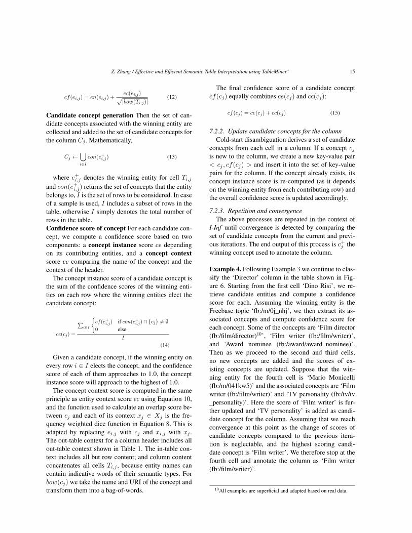
belongs to, I is the set of rows to be considered. In caseof a sample is used, I includes a subset of rows in thetable, otherwise I simply denotes the total number ofrows in the table.Confidence score of concept For each candidate con-cept, we compute a confidence score based on twocomponents: a concept instance score ce dependingon its contributing entities, and a concept contextscore cc comparing the name of the concept and thecontext of the header.
The concept instance score of a candidate concept isthe sum of the confidence scores of the winning enti-ties on each row where the winning entities elect thecandidate concept:
ce(cj) =
∑i∈I
{cf(e+
i,j) if con(e+i,j) ∩ {cj} 6= ∅
0 else
I
(14)
Given a candidate concept, if the winning entity onevery row i ∈ I elects the concept, and the confidencescore of each of them approaches to 1.0, the conceptinstance score will approach to the highest of 1.0.
The concept context score is computed in the sameprinciple as entity context score ec using Equation 10,and the function used to calculate an overlap score be-tween cj and each of its context xj ∈ Xj is the fre-quency weighted dice function in Equation 8. This isadapted by replacing ei,j with cj and xi,j with xj .The out-table context for a column header includes allout-table context shown in Table 1. The in-table con-text includes all but row content; and column contentconcatenates all cells Ti,j , because entity names cancontain indicative words of their semantic types. Forbow(cj) we take the name and URI of the concept andtransform them into a bag-of-words.
The final confidence score of a candidate conceptcf(cj) equally combines ce(cj) and cc(cj):
cf(cj) = ce(cj) + cc(cj) (15)
7.2.2. Update candidate concepts for the columnCold-start disambiguation derives a set of candidate
concepts from each cell in a column. If a concept cjis new to the column, we create a new key-value pair< cj , cf(cj) > and insert it into the set of key-valuepairs for the column. If the concept already exists, itsconcept instance score is re-computed (as it dependson the winning entity from each contributing row) andthe overall confidence score is updated accordingly.
7.2.3. Repetition and convergenceThe above processes are repeated in the context of
I-Inf until convergence is detected by comparing theset of candidate concepts from the current and previ-ous iterations. The end output of this process is c+j thewinning concept used to annotate the column.
Example 4. Following Example 3 we continue to clas-sify the ‘Director’ column in the table shown in Fig-ure 6. Starting from the first cell ‘Dino Risi’, we re-trieve candidate entities and compute a confidencescore for each. Assuming the winning entity is theFreebase topic ‘fb:/m/0j_nhj’, we then extract its as-sociated concepts and compute confidence score foreach concept. Some of the concepts are ‘Film director(fb:/film/director)10’, ‘Film writer (fb:/film/writer)’,and ‘Award nominee (fb:/award/award_nominee)’.Then as we proceed to the second and third cells,no new concepts are added and the scores of ex-isting concepts are updated. Suppose that the win-ning entity for the fourth cell is ‘Mario Monicelli(fb:/m/041kw5)’ and the associated concepts are ‘Filmwriter (fb:/film/writer)’ and ‘TV personality (fb:/tv/tv_personality)’. Here the score of ‘Film writer’ is fur-ther updated and ‘TV personality’ is added as candi-date concept for the column. Assuming that we reachconvergence at this point as the change of scores ofcandidate concepts compared to the previous itera-tion is neglectable, and the highest scoring candi-date concept is ‘Film writer’. We therefore stop at thefourth cell and annotate the column as ‘Film writer(fb:/film/writer)’.
10All examples are superficial and adapted based on real data.

16 Z. Zhang / Effective and Efficient Semantic Table Interpretation using TableMiner+
7.3. Preliminary cell disambiguation
Next, c+j is used as constraint to perform prelimi-nary cell disambiguation in the column. The processre-starts from the first cell in the column. For cells thathave already passed a cold-start disambiguation pro-cess during preliminary column classification, we sim-ply need to re-select the highest scoring candidate en-tities satisfying the condition: con(ei,j) ∩ {c+j } 6= ∅.For any new cells, disambiguation follows the sameprocedure as cold-start disambiguation (Section 7.2.1)with one modification: candidate generation uses c+j asa filter to select only entities that are associated withc+j as disambiguation candidates. Compared to the ex-haustive strategy adopted by state-of-the-art methods,this reduces computation by cutting down the numberof candidate entities for consideration.
Disambiguation of each new cell generates a set ofconcepts, of which some can be new while others mayalready exists in Cj . By the end of the process, Cjis updated by: (1) adding newly derived concepts; (2)for those already exist in Cj at the beginning, revisingtheir confidence scores. This changes Cj and in somecases, causes the winning concept for the column tobe inconsistent from that at the beginning of the pre-liminary cell disambiguation stage. This is handled bythe UPDATE phase to be discussed in the followingsection.
Example 5. Following Example 4, we use ‘Film writer(fb:/film/writer)’ as constraint to disambiguate thecells in the column. For the four cells already pro-cessed in Example 4, we simply re-select from theircandidate entities the highest scoring one that is alsoan instance of this concept. To disambiguate the newcell ‘Nanni Loy’, we only consider candidate enti-ties that are instances of the concept for the col-umn:‘Film writer’. Assuming that the winning entityis ‘fb:/m/02qmpfs’. Then its associated concepts ‘Filmwriter’, ‘Film director (fb:/film/director)’, ‘Film actor(fb:/film/actor)’ are used to further update the candi-date concepts on the column. At the end of the process,it is likely that the highest scoring concept for the col-umn has changed to ‘Film director (fb:/film/director)’.
8. NE-Column interpretation - the UPDATE phase
Once the LEARNING phase is applied to all NE-columns in the table, the UPDATE phase begins to en-force interdependence between classification and dis-
ambiguation within each column as well as across dif-ferent columns. This is done by an iterative optimiza-tion process shown in Algorithm 2. Note that our previ-ous work [42] only captures interdependence betweenclassification and disambiguation within each separatecolumn. Here we improve it by also capturing cross-column interdependence with a notion of ‘domain con-sensus’.
Algorithm 2 UPDATE1: Input: C, E , prev_C ← ∅, prev_E ← ∅2: while stabilized(C, E , prev_C, prev_E)=false do3: prev_C ← C, prev_E ← E4: bow(domain)← domainrep(E)5: for all Cj ∈ C do6: for all cj ∈ Cj do7: cf(cj) = ce(cj) + cc(cj) + dc(cj)8: end for9: c+j ← electConcept(Cj)
10: Cj , Ei,j ← disambiguate(Ti,j , c+j )11: update(Cj , C, Ei,j , E)12: end for13: end while
8.1. Domain representation
In each iteration, the process starts with creating abag-of-words representation of the domain using thewinning entities from all cells (E) in the table at thecurrent iteration (line 4 in Algorithm 2):
bow(domain)←⋃i,j
defbow(e+i,j) (16)
where defbow denotes ‘definitional’ bag-of-words,and takes a definitional sentence about an entity andconverts it into a bag-of-words representation in thesame way as bow(·). A definitional sentence is com-monly found in almost any knowledge base. For exam-ple, WordNet has a one-sentence definition for everysynset; the first sentence in an Wikipedia article usu-ally defines an entity [16]; this also applies to the de-scription of a Freebase topic (e.g., a concept or namedentity) or a DBpedia resource. The idea is that the def-initional sentence provides a focused description ofthe entity, likely to contain informative words aboutthe general domain it is related to. In particular, it of-ten contains words forming hypernymy relation withthe entity [16,44]. For example, the Freebase defini-tional sentence about the English city ‘Sheffield’ con-

Z. Zhang / Effective and Efficient Semantic Table Interpretation using TableMiner+ 17
tains words11 ‘city’, ‘metropolitan’, ‘borough’, ‘York-shire’, and ‘England’, which are useful words definingthe concept space of the entity.
8.2. Column annotation revision
The bag-of-words representation of the domain isthen used to revise the concept annotations on all NE-columns (C). To do so, we compute a domain consen-sus score dc for each candidate concept from each NE-column, and add this to their overall confidence score(line 7 in Algorithm 2). The domain consensus scoreis based on the frequency weighted dice overlap be-tween the bag-of-words representations of the conceptand the domain.
dc(cj) =√dice(cj , domain) (17)
Since the sizes of bow(cj) and bow(domain) areoften different orders of magnitude, square root isused to balance the score. Also domain consensusis computed with respect to entities from all cellsfrom any columns, which serves as a way of ensur-ing inter-column dependence. After revising the confi-dence scores of candidate concepts, the winning con-cepts for each column are re-selected (Line 9).
8.3. Cell annotation revision
For any column, if the new winning concept is dif-ferent from the that generated in the previous itera-tion, the disambiguation result on that column is re-vised (Line 10). This follows the procedure of prelim-inary cell disambiguation (Section 7.3).
These updating processes are repeated until all an-notations are stabilized. Specifically, in each iterationfunction stabilized checks the winning concepts forall NE-columns and the winning entities for all cells inthe previous iteration against those in the current itera-tion. The UPDATE process is called to be stabilized ifno difference is detected.
Note that re-computing disambiguation and classifi-cation may require retrieving data of new entity candi-dates from the knowledge base and subsequently con-structing their feature representation for disambigua-tion due to the possible change of c+j at each itera-tion. However, this design still largely improves theexhaustive strategy because: (1) empirically the UP-
11http://www.freebase.com/m/0m75g, last retrieved on 13 April2014.
DATE phase stabilizes fast and in most cases involvesmerely re-selecting those ‘losing’ candidate entitiesthat were already seen in the LEARNING phase; (2)when new candidates are indeed added it only happensin significantly fewer cells than the entire column thatan exhaustive strategy would otherwise have to dealwith.
Example 6. Following Example 5, assuming we haveannotated all NE-columns and their cells (also see d6
in Figure 2). We begin the UPDATE process by tak-ing the winning entity annotations from columns 1, 3,and 4 in the Table shown in Figure 6 to create a bag-of-words representation of the domain. Again usingthe ‘Director’ column, we proceed to compute a do-main consensus score for each candidate concept forthis column (i.e., ‘Film director’, ‘Film writer’ etc) andupdate their confidence scores. The winning conceptis re-selected, which we assume is changed to ‘Filmdirector’. This is different from that at the beginning(‘Film writer’). Therefore, we take the new conceptand use it to revise cell annotations in the column. Wedo this for the other two columns and repeat this pro-cess until all annotations are no longer changed.
9. Relation enumeration and annotatingliteral-columns
9.1. Relation enumeration
Relation enumeration firstly begins by interpretingrelations between the subject column and any othercolumns on each row independently. Let Tj be thesubject column in a table and Tj′ denote any othercolumns. Given the winning subject entity e+
i,j for cellTi,j and Ti,j′(j 6= j′) as another cell on the samerow, the candidate set of relations between Ti,j andTi,j′ , denoted by Rij,j′ , is derived from the triplescontaining e+
i,j as subject, denoted by Ψi,j = {<e+i,j , predicate, object >}. Then let ψi,j ∈ Ψi,j be
one of the triples, and functions p(ψi,j), o(ψi,j) returnthe predicate and object from the triple respectively,the candidate relations Rij,j′ is the set of unique predi-cates in Ψi,j , i.e., {p(ψi,j)|∀ψi,j ∈ Ψi,j}.
Then a confidence score is computed for each can-didate relation rij,j′ ∈ Rij,j′ . To do so, the subset oftriples from Ψi,j containing rij,j′ as predicate are se-lected. Then the object of each triple in this set ismatched against the content in Ti,j′ using the fre-
18 Z. Zhang / Effective and Efficient Semantic Table Interpretation using TableMiner+
quency weighted dice function (Equation 8), and thehighest score is assigned to be the confidence score forthe candidate relation:
cf(rij,j′) =
maxψi,j∈Ψi,j ,p(ψi,j)=ri
j,j′
dice(Ti,j′ , o(ψi,j))(18)
where function dice(Ti,j′ , o(ψi,j)) computes anoverlap score between the bag-of-words representa-tions of the cell and the object of a triple that containsrij,j′ as predicate. The winning relation for the row isdenoted by ri+j,j′ .
After the winning relation is computed for each rowbetween Tj and Tj′ , the candidate set of relations forthe two columns R(j, j′) is derived by collecting thewinning relations on all rows:
R(j, j′)←⋃i
ri+i,j′ (19)
Then a confidence score is computed for each in-stance rj,j′ ∈ R(j, j′), and it consists of two parts:a relation instance score re and a relation contextscore. The relation instance score is computed in thesame way as concept instance score:
re(rj,j′) =
∑i
{cf(ri+j,j′) if ri+j,j′ ≡ rj,j′0 else
|{Ti}|(20)
where i denotes the row index of the table and |{Ti}|returns the number of rows in the table.
The relation context score is computed in the sameway as entity context score using Equation 10, and thefunction used to calculate an overlap score betweenrj,j′ and each of its context is the frequency weighteddice function in Equation 8. This is adapted by re-placing ei,j with rj,j′ and xi,j with xj,j′ . The bag-of-words representation bow(rj,j′) is based on l(rj,j′)which returns the name and URI of the relation. Thecontext of a relation includes column header (whichsometimes indicates the relation with the subject col-umn), surrounding paragraphs and semantic markups.Other types of context are less likely to contain men-tions of relations.
The final confidence score of a candidate relationadds up its instance and context score with equalweights, and the final binary relation that associatessubject column Tj with column T ′j is the candidatewith the highest confidence score.
Example 7. Assuming the entity annotation for cellT3,1 in the table of Figure 6 is ‘A Difficult Life(fb:/m/02qlhz2)’, which has two triples<fb:/m/02qlhz2,fb:/film/film/directed_by, ‘Dino Risi’> and <fb:/m/02qlhz2, fb:/film/film/starring, ‘Dino Sordi’>. To pre-dict the relation between columns T1 and T3 on thisrow, the object values of the two triples are matchedagainst the text value ‘Dino Risi’ in cell T3,3 based onoverlap. Then the first triple will receive a score of 1.0while the second 0.5. Hence the relation between thetwo columns elected by this row (r3+
1,3) is the predicate‘fb:/film/film/directed_by’ and cf(r3+
1,3) = 1.0. Nextwe repeat this process for the remaining rows to elect arelation for every other row between the two columns,and the set of all these relations become R3,3. Sup-pose that r4+
1,3 is also ‘fb:/film/film/directed_by’ andcf(r4+
1,3) = 0.9. Then to compute the overall confi-dence score of ‘fb:/film/film/directed_by’ across thetwo columns, the relation instance score adds up thetwo values and become 1.9. We then calculate the re-lation context score and add it to the instance score toderive the final score.
9.2. Labeling literal-columns
Literal-columns are expected to contain attributedata of entities in the subject column. They do not de-note entities and therefore, cannot be interpreted us-ing the column interpretation method described above.In previous work [21,7,25,23,24] they are simply ig-nored. This work also assigns a column annotation thatbest describes the attribute data in literal-columns.
Given a literal-column T ′j that forms a binary rela-tion rj,j′ with the subject column Tj , the annotationfor this column is simply l(rj,j′), since rj,j′ typicallydescribes a property of the subject column concept insuch cases.
10. Experiment settings
Semantic Table Interpretation can be evaluated byboth in-vitro (assessing the annotations directly) andin-vivo (assessing the accuracy of applications built ontop of the annotations) experiments. In this work, weuse in-vitro experiments because (1) they are the mostcommonly used evaluation approach and (2) standarddatasets are available.

Z. Zhang / Effective and Efficient Semantic Table Interpretation using TableMiner+ 19
10.1. Knowledge base and datasets
We use Freebase as the knowledge base for Seman-tic Table Interpretation, as it is currently the largestknowledge base and linked data set in the world. Itcontains over 3.1 billion facts about over 58 milliontopics (e.g., entities, concepts), significantly exceed-ing other popular knowledge bases such as DBpediaand YAGO. Further it has direct mappings to resourcesfrom other datasets, making them easier to be used asgold standard. For evaluation, we compiled and an-notated four datasets using Freebase: Limaye200, Li-mayeAll, IMDB and MusicBrainz. To the best ofour knowledge, this is the largest dataset for this taskand we make them available to encourage comparativestudies12.
10.1.1. LimayeAll and Limaye200These datasets are the rebuilt versions of the origi-
nal four datasets used by Limaye et al. [21]. The orig-inal datasets consist of over 6,000 tables, 94% col-lected from Wikipedia and the rest from the generalWeb. Entities in the tables were annotated with linksto Wikipedia articles; columns and binary relations be-tween columns were annotated by concepts and rela-tions in the YAGO knowledge base (2008 version).
These datasets are re-created for a number ofreasons. First, Wikipedia has undergone significantchanges since the publication of the datasets such thata large proportion of the source webpages - as wellas the contained tables - have been changed. Second,we notice that the original ground truth for named en-tity disambiguation were very sparse and possibly bi-ased. As shown in Appendix C, it is less well-balancedthan the re-created dataset and a simple exact namematch baseline has achieved significantly higher accu-racy than the original reported results in Limaye et al.[21]. Third, this work uses a different knowledge basefrom YAGO, such that the original ground truth cannotbe directly used.Entity ground truth - LimayeAll We run a processto automatically update the webpages in the originaldataset and re-annotate entity cells by mapping the
12Please contact the author on how to obtain, as the dataset is verylarge. Although Freebase has been closed, this work was however,first submitted in May 2013, at which time the close-down of Free-base was not foreseeable. To enable comparative studies, we also re-lease cached Freebase data for this work. Also the current API onGitHub implements an interface with DBpedia, and a plan is madeto migrate relevant software to the Google Knowledge Graph oncean appropriate API is available.
original Wikipedia ground truth to Freebase. Details ofthis process is described in Appendix B.Column annotation and relation ground truth - Li-maye200 To create the ground truth for evaluatingcolumn classification and relation enumeration, a ran-dom set of 200 tables are drawn from the LimayeAlldataset. These tables are firstly manually examinedto identify subject columns, then annotated followinga similar process as Venetis et al. [35]. Specifically,TableMiner+ and the baselines (Section 10.3) are runon these tables and the candidate concepts for all tablecolumns and relations between the subject column andother columns in each table are collected and presentedto annotators. The annotators mark each label as ‘best’,‘okay’, or ‘incorrect’. The basic principle is to preferthe most specific concept/relation among all suitablecandidates. For example, given a cell ‘Penrith Pan-thers’, the concept ‘Rugby Club’ is the ‘best’ candidateto label its parent column while ‘Sports Team’ and ‘Or-ganization’ are ‘okay’. The annotators may also insertnew labels if none of the candidates are suitable.
10.1.2. IMDBThe IMDB dataset contains over 7,000 tables ex-
tracted from a random set of IMDB movie webpages.Each IMDB movie webpage13 contains a table listing a‘cast’ column of actors/actresses and a column of cor-responding characters played. Cells in the actor/actresscolumn are linked with an IMDB item id, which, whensearched in Freebase, returns a unique (if any) mappedFreebase URI. Thus entities in these columns are an-notated automatically in such a way. The ‘character’column is not used since they are not mapped in Free-base. The cast column is also manually labeled with‘best’ and ‘okay’ concepts in the same way as for Li-maye200. No subject column or relations are annotatedbecause only one column is considered in this dataset.
10.1.3. MusicBrainzThe MusicBrainz dataset contains some 1,400 tables
extracted from a random set of MusicBrainz recordlabel webpages. Each MusicBrainz record label web-page14 contains a table listing the music released bya production company. Each webpage uses paginationto separate very large tables, and only the first pageis downloaded. The table typically has 8 columns, ofwhich one lists music release titles (subject column)and one lists music artists. Each release title or artist
13E.g., http://www.imdb.com/title/tt0071562/14E.g., http://musicbrainz.org/label/9e6b4d7f49584db78504-
d89e315836af

20 Z. Zhang / Effective and Efficient Semantic Table Interpretation using TableMiner+
has a MusicBrainz id, which can be mapped to a Free-base URI in the same way as for the IMDB dataset.Thus entities in these two columns are annotated insuch a way. Then the table columns and binary rela-tions between the subject column and others are alsoannotated manually following the same procedure asfor IMDB and Limaye200.
10.1.4. Dataset statisticsTable 3 shows general statistics of the datasets. Fig-
ure 7 shows the distribution of rows and columnscontaining entity annotations in the ground truth, andlength of text in cells by number of tokens. Tables inMusicBrainz contain no more than 50 rows becauseof the pagination on the webpage and only the firstpage is downloaded. The IMDB entity ground truth hasonly 1 column in every table; while for MusicBrainz,this is either 1 or 2 columns. Very long cell text isfound to be rare in LimayeAll, but slightly more fre-quent in MusicBrainz due to long names of classicmusic titles. Cells in IMDB tables are typically per-son names and usually contains 1 or 2 tokens. Ar-guably, LimayeAll and Limaye200 are the most di-verse datasets, since they cover a significantly largernumber of domains and more diverse table structuresand schemata, whereas IMDB and MusicBrainz eachcontains only one table structure and schema.
Table 4 compares against datasets used by otherstudies. Arguably, TableMiner+ is evaluated using themost comprehensive collection of datasets known todate.
10.2. Evaluation metrics
Effectiveness - Subject column detection is evaluatedby Precision. Then the three annotation tasks of Se-mantic Table Interpretation are evaluated using thestandard Precision, Recall and F1 measures. SinceTableMiner+ ranks candidates by scores, only the high-est ranked prediction by TableMiner+ is considered.Each ‘best’ label is awarded a score of 1 while each‘okay’ label is awarded 0.5. Further, if there are mul-tiple highest-ranked candidates, each candidate con-sidered correct only receives a fraction of its score as
score#topranked . For example, if a column containing filmtitles has two concept candidates with the same highestscore: ‘Film’ (best) and ‘Book’ (incorrect), this pre-diction receives a score of 0.5 instead of 1. This isto penalize the situation where the Semantic Table In-terpretation system fails to discriminate false positivesfrom true positives. From a knowledge base population
point of view, false positives cause incorrect triples tobe populated into knowledge bases and the LOD cloud.
For column classification and relation enumeration,evaluation reports results under both ‘strict’ and ‘tol-erant’ mode. To evaluate column classification, thestrict mode only considered ‘best’ annotations; whilethe tolerant mode considers both ‘best’ and ‘okay’ an-notations. Evaluating relation enumeration under thestrict mode only considers relations between subjectcolumn and other columns in a table, and only ‘best’annotations are included. Under the tolerant mode,in addition to also including ‘okay’ annotations, ifTableMiner+ predicts correct relations between non-subject columns or the reversed relation between thesubject column and other columns, then each predic-tion is awarded a score of 0.5.
Moreover, since most state-of-the-art methods havefocused on only NE-columns, we report results ob-tained on NE-columns as well as both NE- and literal-columns for column classification and relation enu-meration.The efficiency of TableMiner+ is assessed by empiricalwall-clock time and savings in terms of candidate en-tities needed to be considered for disambiguation. Asdiscussed before, retrieving candidate entities and theirdata, constructing feature space and computing sim-ilarities consume the large majority of time. A morereliable way of improving efficiency is thus reducingthe size of the candidate space. To reduce network la-tency we use a caching mechanism in each compara-tive model and TableMiner+ (see Section 10.3). Specif-ically, when a request to the knowledge base is sent forthe first time, we cache the query results locally. Thenall subsequent identical requests will only be served bythe local cache.
10.3. Comparative models and configurations
TableMiner+ is evaluated against four baseline meth-ods and two re-implemented state-of-the-art methods.The implementation of all these methods are releasedon GitHub15.
10.3.1. BaselinesEach baseline starts with the same subject column
detection component, but uses different methods fordisambiguating entity cells, classifying columns, andannotating relations between subject column and othercolumns.
15https://github.com/ziqizhang/sti

Z. Zhang / Effective and Efficient Semantic Table Interpretation using TableMiner+ 21
Table 3Statistics of the datasets for evaluation. ‘All’ under ‘Labeled columns’ shows the number of both labeled NE- and literal-columns, while ‘NE’refers to only NE-columns. Likewise ‘All’ under ‘Labeled relations’ shows the number of labeled relations between subject columns and eitherNE- or literal columns, while ‘NE’ refers to only relations with NE-columns.
Dataset Tables Subject column Entities Labeled columns Labeled relationsAll NE All NE
Limaye200 200 X - 615 415 361 204LimayeAll 6,310 227,046 - - - -IMDB 7,416 92,321 7,416 7,416 - -MusicBrainz 1,406 X 93,266 9,842 4,218 7,030 5,624
Fig. 7. Dataset statistics (min., max. avg. (black diamonds), kth quantile): #r - number of rows; #nec - number of columns containing annotatednamed entities in ground truth; cl - content cell text length in terms of number of tokens delimited by non-alphanumeric characters.
Table 4Comparison against datasets used by state-of-the-art. ‘-’ indicates unknown or not clear.
Method Dataset Tables Columns Entities Relations
TableMiner+
Limaye200 200 615 - 361LimayeAll 6,310 - 227,046 -IMDB 7,416 7,416 92,321 -MusicBrainz 1,406 9,842 93,266 -
Hignette et al. [14,15] 1 dataset - 81 - -Limaye et al. [21] 4 datasets 6,310 747 142,737 90Syed et al. [7] 1 dataset 5 21 171 -Venetis et al. [35] 1 dataset 168 - - -Buche et al. [2] 1 dataset 90 81 - 316Mulwad et al. [24] 1 dataset 203-490 - - -Zhang [42] 2 datasets 7,446 7,608 94,406 -Zhang [41] 2 datasets 6,310 615 227,046 -
Baseline ‘name match’ Bnm firstly disambiguates ev-ery cell in an NE-column by retrieving candidate enti-ties from Freebase using the text content in the cell asquery, then selecting a single entity: the highest rankedcandidate whose name matches exactly the cell text.If no candidates are found to match, the top-ranked
candidate is chosen. Freebase adopts a ranking algo-
rithm that reflects both the relevance and popularity of
a topic in the knowledge base.
Next, to classify the NE-column with a concept, en-
tities from each cell cast a vote for the concepts they
22 Z. Zhang / Effective and Efficient Semantic Table Interpretation using TableMiner+
are associated to, and the one receiving the most votesis chosen as the annotation for the column.
Relation enumeration follows a similar procedure.Candidate relations on each row is derived and theirscores computed in the same way as TableMiner+
(Section 9.1, Equation 18). Then each candidate with ascore greater than 0 is selected from the row and con-sidered as a candidate relation for the two columns andcasts a vote toward the candidate. The best relationsfor the two columns are those receiving the most votes.
Literal-columns are annotated the same way asTableMiner+ (Section 9.2).Baseline ‘similarity-based’ firstly disambiguates ev-ery cell in an NE-column, then derives column anno-tations based on the winning entity from every cell.
For cell disambiguation, we compute a score foreach candidate entity as the sum of a simple contextscore and the string similarity between the name of thecandidate and the cell text. The context score is com-puted using Equation 9, where x is the row contentonly.
For column classification, candidate concepts for anNE-column are firstly gathered based on the winningentities from each cell. The final score of a candidateconcept consists of two parts: (1) the number of win-ning entities associated with the concept normalizedby the number of rows in the table, and (2) a stringsimilarity score between the concept’s name and theheader text (if exists).
For relation enumeration and the annotation ofliteral-columns, we use the same procedures from thename match baseline Bnm.
To compute string similarity, we test three metricsand therefore create three similarity baselines: Cosine(Bcos), Dice (Bdice) coefficient, and Levenshtein (Blev).
The key differences between the four baselines andTableMiner+ are: (1) TableMiner+ uses out-table con-text while the baselines do not; (2) TableMiner+ adoptsa bootstrapping, incremental approach with an itera-tive, recursive optimization process to enforce inter-dependence between different annotation tasks. Thebaselines however, use an exhaustive strategy and arebased on very simple interdependence (i.e., both rela-tion enumeration and column classification depend oncell disambiguation).
10.3.2. Re-implementation of state-of-the-artWe re-implemented two state-of-the-art methods
and adapted them to Freebase as there are no existingsoftware that can be directly used, and also differentknowledge bases have been used in the original work.
We choose to implement the methods by Limaye et al.[21] and Mulwad et al. [24], as they are able to addressall three annotation tasks in Semantic Table Interpreta-tion. Re-implementation of these methods is not a triv-ial task. First, the use of different knowledge bases im-plies that certain features used in the original work areunavailable, must be adapted or replaced. Second, eachmethod has used in-house tools for pre-processing ortraining. Therefore, our re-implementation has focusedon the core inference algorithm in the two methods.We advise readers that the re-implementation is notguaranteed to be an identical replication of the originalsystems. We describe details of re-implementation inAppendix D, and here we summarize key points. Notethat both methods can only deal with NE-columns.Limaye et al. (Limaye2010) model a table as a factorgraph and apply joint inference to solve the three anno-tation tasks simultaneously. A factor encodes the com-patibility between a variable (e.g., a cell) and its can-didates (e.g., candidate entities), or between variablesbelieved to be interdependent. In the original work, thecompatibility is calculated based on a number of fea-tures, the weight of which is learned using a super-vised model. Our implementation16 simply uses equalweights. Further, we discard all relation variables andonly build a smaller factor graph of concept and en-tity variables. This is because empirically, we have no-ticed that adding relation variables caused drop in theaccuracy of column classification (see Appendix D).Mulwad et al. model a table using a similar factorgraph, then apply a light-weight inference algorithmbased on semantic message passing. Their method de-pends on a pre-process that disambiguates entity cells(i.e., the so-called ‘entity ranker’). This process usesa supervised model built on features that are specificto the knowledge bases used in the original work. Wecreate two models each with a different substitute ofthe ‘entity ranker’. Mulwad2013 uses a simple rankerthat linearly combines features equivalent to thoseused in the original work (but derived from Freebase)to score and rank candidate entities. Mulwad2013tm+
uses TableMiner+’s formula of entity confidence score(cf(ei,j) in Section 7.2.1) to score and rank candidateentities.
16We used Mallet GRMM: http://mallet.cs.umass.edu/grmm/
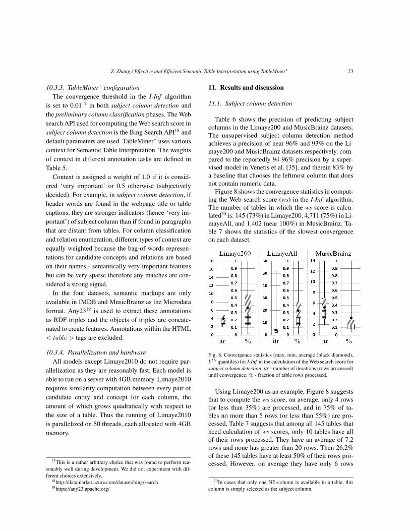
Z. Zhang / Effective and Efficient Semantic Table Interpretation using TableMiner+ 23
10.3.3. TableMiner+ configurationThe convergence threshold in the I-Inf algorithm
is set to 0.0117 in both subject column detection andthe preliminary column classification phases. The Websearch API used for computing the Web search score insubject column detection is the Bing Search API18 anddefault parameters are used. TableMiner+ uses variouscontext for Semantic Table Interpretation. The weightsof context in different annotation tasks are defined inTable 5.
Context is assigned a weight of 1.0 if it is consid-ered ‘very important’ or 0.5 otherwise (subjectivelydecided). For example, in subject column detection, ifheader words are found in the webpage title or tablecaptions, they are stronger indicators (hence ‘very im-portant’) of subject column than if found in paragraphsthat are distant from tables. For column classificationand relation enumeration, different types of context areequally weighted because the bag-of-words represen-tations for candidate concepts and relations are basedon their names - semantically very important featuresbut can be very sparse therefore any matches are con-sidered a strong signal.
In the four datasets, semantic markups are onlyavailable in IMDB and MusicBrainz as the Microdataformat. Any2319 is used to extract these annotationsas RDF triples and the objects of triples are concate-nated to create features. Annotations within the HTML< table > tags are excluded.
10.3.4. Parallelization and hardwareAll models except Limaye2010 do not require par-
allelization as they are reasonably fast. Each model isable to run on a server with 4GB memory. Limaye2010requires similarity computation between every pair ofcandidate entity and concept for each column, theamount of which grows quadratically with respect tothe size of a table. Thus the running of Limaye2010is parallelized on 50 threads, each allocated with 4GBmemory.
17This is a rather arbitrary choice that was found to perform rea-sonably well during development. We did not experiment with dif-ferent choices extensively.
18http://datamarket.azure.com/dataset/bing/search19https://any23.apache.org/
11. Results and discussion
11.1. Subject column detection
Table 6 shows the precision of predicting subjectcolumns in the Limaye200 and MusicBrainz datasets.The unsupervised subject column detection methodachieves a precision of near 96% and 93% on the Li-maye200 and MusicBrainz datasets respectively, com-pared to the reportedly 94-96% precision by a super-vised model in Venetis et al. [35], and therein 83% bya baseline that chooses the leftmost column that doesnot contain numeric data.
Figure 8 shows the convergence statistics in comput-ing the Web search score (ws) in the I-Inf algorithm.The number of tables in which the ws score is calcu-lated20 is: 145 (73%) in Limaye200, 4,711 (75%) in Li-mayeAll, and 1,402 (near 100%) in MusicBrainz. Ta-ble 7 shows the statistics of the slowest convergenceon each dataset.
Fig. 8. Convergence statistics (max, min, average (black diamond),kth quantiles) for I-Inf in the calculation of the Web search score forsubject column detection. itr - number of iterations (rows processed)until convergence; % - fraction of table rows processed.
Using Limaye200 as an example, Figure 8 suggeststhat to compute the ws score, on average, only 4 rows(or less than 35%) are processed, and in 75% of ta-bles no more than 5 rows (or less than 55%) are pro-cessed. Table 7 suggests that among all 145 tables thatneed calculation of ws scores, only 10 tables have allof their rows processed. They have an average of 7.2rows and none has greater than 20 rows. Then 26.2%of these 145 tables have at least 50% of their rows pro-cessed. However, on average they have only 6 rows
20In cases that only one NE-column is available in a table, thiscolumn is simply selected as the subject column.

24 Z. Zhang / Effective and Efficient Semantic Table Interpretation using TableMiner+
Table 5Different context weight used in different components.
Component In-table context Out-table contextcolumnheader
rowcontent
columncontent
webpagetitle
table caption/title paragraphs
semanticmarkups
Sub.Col. detection §6.2 - - - 1.0 1.0 0.5 -Entity context score §7.2.1 1.0 1.0 0.5 1.0 1.0 0.5 1.0Concept context score §7.2.1 1.0 - 1.0 1.0 1.0 1.0 1.0Relation context score §9.1 1.0 - - - - 1.0 1.0
Table 6Subject column detection results in Precision
Dataset Tables PrecisionLimaye200 200 95.5MusicBrainz 1406 92.7
Table 7Statistics of the slowest convergence in the calculation of the Websearch score for subject column detection.
Limaye200 LimayeAll MusicBrainz100% of rows processed in
% of tables 6.9% 5.9% 6.5%Avg. rows 7.2 6.5 4.6Rows >20 0 4 0
>50% of rows processed in% of tables 26.2% 19.8% 12.6%Avg. rows 6.0 6.0 5.2Rows >20 0 7 0
and none of them have greater than 20 rows. Thesefigures suggest potentially significant improvement inefficiency over an exhaustive approach that computesthe ws score using all rows in tables. The figures onthe LimayeAll and MusicBrainz datasets suggest evengreater savings. Consider that typical Web search APIsare quota-limited and pay-per-use, and it is extremelyexpensive (if not impossible) to run a local search en-gine on a reasonable sample of the entire Web. We be-lieve that the I-Inf algorithm delivers substantial bene-fits in the task of subject column detection.
Manual inspection shows that in most cases the er-rors fall under several categories. The first is due to du-plicate values in subject columns. An extreme exam-ple is the disambiguation table discussed before (i.e.,‘List of peaks named Bear Mountain’), in which thesubject column contains only a single unique value.The second is caused by long-named entities in sub-ject columns. For example, the subject column in theMusicBrainz tables lists titles of music releases, some
of which has a name consisting of more than 10 to-kens. This severely penalizes their context match cmand ws scores as it is unlikely to find exact match oftheir names in table context and search result docu-ments. The third category includes arguable (few) ta-bles that in strict terms, do not necessarily have a sub-ject column. This includes tables listing events, such aslap records of racing car drivers in a particular tourna-ment. In these cases, annotators typically selected theleftmost NE-column.
11.2. Effectiveness
11.2.1. Against baselinesTables 8, 9 and 10 compare TableMiner+ against the
four baselines in the cell disambiguation, column clas-sification and relation enumeration tasks respectively.The highest figures are marked in bold. Overall, it isclear that TableMiner+ always obtains the best perfor-mance in all tasks and on all datasets. It also showsstronger improvement in the classification and relationenumeration tasks.
For disambiguation, even the simplistic baselineBnm obtains surprisingly competitive results on the Li-mayeAll and IMDB datasets. In fact, on the originaldatasets by Limaye et al. [21] Bnm obtains a surpris-ingly high F1 of 92.6, significantly higher than theweighted average21 of 84.1 based on figures reportedin Limaye et al. [21]. As discussed earlier, our analy-sis - shown in Appendix C - suggests that the originaldatasets are sparse and less balanced.
Its highly competitive performance on the IMDBdataset could be explained by the domain and themethod for ranking search results by Freebase. Movieis a highly popular domain representing a fair largeproportion of Freebase. Since Freebase Search APIpromotes popular topics, when a person name is
21Macro-average over all datasets taking into account the size ofeach dataset.

Z. Zhang / Effective and Efficient Semantic Table Interpretation using TableMiner+ 25
Table 8Disambiguation results (F1) on four datasets.
Limaye200 LimayeAll IMDB MusicBrainzBnm 78.3 82.2 92.8 57.0Blev 78 82.1 93.5 84.83Bcos 79.2 82.7 93.4 84.76Bdice 79.9 82.8 93.5 84.84TableMiner+ 82.3 83.7 97.6 84.87
Table 9Classification results (F1) on three datasets.
Bnm Blev Bcos Bdice TableMiner+
Lim
aye2
00 NE-columns onlystrict 23.9 45.4 43.5 48.9 65.8tolerant 48.8 63.8 62.2 66.1 75.0
All columnsstrict 31.4 48.7 46.9 51.3 64.0tolerant 51.1 63.3 61.8 65.0 71.5
IMD
B
NE-/All columnsstrict 22.7 32.3 31.9 32.0 97.0tolerant 60.0 64.6 64.4 64.5 97.2
Mus
icB
rain
z
NE-columns onlystrict 59.1 82.6 83.4 83.9 85.2tolerant 61.7 82.6 83.6 83.9 85.9
All columnsstrict 54.6 72.2 72.6 72.9 74.3tolerant 55.9 72.2 72.7 72.9 74.7
Table 10Relation enumeration results (F1) on two datasets.
Bnm Blev Bcos Bdice TableMiner+
Lim
aye2
00 NE-columns onlystrict 61.3 61.7 61.8 61.8 72.5tolerant 65.8 66.3 66.5 66.4 76.0
All columnsstrict 59.7 61.0 60.6 61.1 66.2tolerant 63.0 64.4 64.1 64.4 68.7
Mus
icB
rain
z
NE-columns onlystrict 63.8 67.2 67.1 67.1 67.9tolerant 65.0 68.3 68.2 68.2 69.1
All columnsstrict 78.7 82.0 81.9 81.9 82.6tolerant 79.2 82.5 82.4 82.4 83.1
searched it is more likely to obtain movie-related top-ics as top results than any other domains. Hence byselecting the top result Bnm is very likely to succeed.
While although music is also a highly popular do-main, Bnm could not replicate similar performance.Manual inspection shows that a fair proportion of mu-sic titles and artists uses very ambiguous names (e.g.,‘Trouble’, a musical release, ‘Pine’, an artist). In con-trast, other baselines perform significantly better byconsidering row content in tables.
Compared to the baselines, TableMiner+ consis-tently obtains the best performance. On the most di-
verse dataset LimayeAll, it improves F1 by between0.9 and 1.5 points. On the MusicBrainz dataset, itmakes little difference from Blev, Bcos, and Bdice. Byexamining the data it is found that the out-table con-text on MusicBrainz webpages are very sparse. In mostcases, the webpage contains only the table. Microdataannotations are also predominantly found inside tablestructures, which are not used by TableMiner+. On thecontrary, the IMDB dataset is completely the opposite:the webpages contain much richer out-table context(including pre-defined Microdata annotations), but lit-tle in-table context as the tables have only two columns

26 Z. Zhang / Effective and Efficient Semantic Table Interpretation using TableMiner+
and neither has column headers. TableMiner+ achievessignificant improvement (between 3.9 and 4.6) overbaselines on IMDB. This strongly suggests that out-table context serves as useful clues for disambiguatingentities in table cells, particularly when in-table con-text is absent. Further, the Microdata-annotations ex-tracted from these webpages could have been a strongcontributor considering that the only difference in out-table context used on LimayeAll and IMDB is that thelatter also uses them as features.
For classification, TableMiner+ in most cases out-performs baselines by a very large margin. Experi-ments on the most diverse dataset Limaye200 see animprovement of between 16.9 and 41.9 under strictmode and 8.9-26.2 under tolerant mode when onlyNE-columns are considered. When all columns are in-cluded, the figures are 12.7-32.6 strict and 6.5-20.4 tol-erant. MusicBrainz sees the smallest improvement ofthe minimum of 1.3 strict and 2.0 (both v.s. Bdice) whenonly NE-columns are considered, or 1.4 strict and 1.8tolerant when all columns are included. This is due tothe same reason behind TableMiner+’s moderate per-formance in the disambiguation task on this dataset:the out-table context is very sparse, thus TableMiner+
in most cases only uses in-table context. Again themost significant improvement is obtained on the IMDBdataset. With the lack of in-table context, particu-larly column headers that are considered a crucial fea-ture in annotating table columns, all baselines performpoorly compared against TableMiner+. TableMiner+
more than tripled their performance under the strictmode and significantly outperforms under the tolerantmode, achieving near-perfect accuracy in both cases.
Also note that the performance by Bnm is generallyinferior on any dataset. This is due to its inability topromote a single top ranked candidate concept in mostcases, or in other words, multiple winning candidatesare penalized by the scoring method. Other baselinesimprove this by also considering the string similaritybetween candidate concept’s label and table columnheaders.
For relation enumeration, on the multi-domain Li-maye200 dataset, an improvement of between 10.7-11.2 strict and 9.5-10.2 tolerant is obtained when onlyrelations between NE-columns are considered. Re-gardless of column types, the figures are 5.1-6.5 strictand 4.3-5.7 tolerant. Improvement on MusicBrainz issmaller: the minimum of 2.8 strict and 0.8 tolerantwith NE-columns only, and the minimum of 0.6 strictand 0.7 tolerant if all columns are included. Again this
could be attributed to the lack of out-table context inthis dataset.
11.2.2. Against state-of-the-artTable 11 shows that TableMiner+ outperforms the
re-implemented state-of-the-art models by a large mar-gin in most cases. Surprisingly, models Limaye2010and Mulwad2013 have underperformed many base-lines in most occasions, particularly in the disambigua-tion task. This may be attributed to two reasons. First,as discussed before, the original work has used knowl-edge base specific features that are unavailable in Free-base, or supervised processes to optimize features.This has made the adaptation work difficult and al-though we have made careful attempt to implement al-ternatives, we cannot guarantee an identical replica-tion of the original methods. Second, we observe thatin the cell disambiguation task, both Limaye2010 andMulwad2013 have only used features that are based onstring similarity metrics. Our similarity baselines (Blev,Bcos, Bdice) also use string similarity features but add animportant type of feature that proves to be very effec-tive: a context score that compares the bag-of-wordsrepresentation of candidate entities of a cell against therow context of the cell.
By using the disambiguation component of Table-Miner+, Mulwad2013tm+ made significant improve-ment over Mulwad2013 on the cell disambiguation andcolumn classification tasks. It also outperforms base-lines in several occasions, but still obtained lower ac-curacy than TableMiner+.
The poor performance of all three models on thecolumn classification task under strict mode is mainlydue to the fact that the algorithms empirically favoredgeneral concepts (‘Person’) over more specific ones(‘Movie Directors’). Again this could be caused by thelack of a clean, strict concept hierarchy that could bemore reliable reference of concept specificity than thealternative features we have to use in Freebase. How-ever, concept hierarchies are not necessarily availablein all knowledge bases. Nevertheless, TableMiner+ isable to predict a single best concept candidate in mostcases without such knowledge. Additionally, the ex-tremely poor accuracy on the IMDB dataset under thestrict mode is largely because all tables in the datasetshare the same schema.
We must re-iterate that despite our best effort, there-implementation is not identical to the original worksdue to many reasons stated above. Hence following thepractice adopted by Mulwad et al. [24], we also com-pare against state-of-the-art using reported figures in

Z. Zhang / Effective and Efficient Semantic Table Interpretation using TableMiner+ 27
Table 11Comparison (F1) against the two re-implemented state-of-the-art (NE-columns only). Note that the re-implementation is not guaranteed to beidentical to the original works due to reasons such as the use of specific tools, change of knowledge bases and datasets.
Limaye2010 Mulwad2013 Mulwad2013tm+ TableMiner+
Dis
ambi
g. Limaye200 - 64.3 68.3 80.2 82.3LimayeAll - 66.0 70.1 81.9 83.7IMDB - 80.6 76.0 96.0 97.6MusicBrainz - 66.4 73.4 83.0 84.87
Cla
ssifi
catio
n Limaye200strict 28.4 30.5 37.4 65.8tolerant 51.9 52.3 58.9 75.0
IMDBstrict 1.7 15.1 59.8 97.0tolerant 49.3 55.2 78.2 97.2
MusicBrainzstrict 72.4 65.6 71.0 85.2tolerant 72.4 74.2 79.3 85.9
Rel
atio
n
Limaye200strict - 55.9 55.1 72.5tolerant - 60.5 58.5 76.0
MusicBrainzstrict - 60.5 49.5 67.9tolerant - 67.6 62.7 69.1
Table 12TableMiner+ on Limaye200 (classification and relation enumeration)and LimayeAll (disambiguation) and state-of-the-art reported figures.All results are based on NE-columns only. [24] and [35] report resultsunder tolerant mode only, weigted average are used where necessary.
Disamb. Class. RelationTableMiner strict
83.765.8 72.5
TableMiner tolerant 75.0 76.0Limaye et al. [21] 84.1 44.5 58.3Mulwad et al. [24] 75.9 54.9 83.5Venetis et al. [35] - 68.6 54.8
Table 12. As it is shown, TableMiner+ has obtainedvery competitive results.
11.2.3. RemarkOverall, we believe these results are very positive.
The rich context model adopted by TableMiner+ -especially the usage of out-table context - enablesTableMiner+ to achieve the best performance in alltasks, and significantly outperform both baseline andstate-of-the-art methods that ignore out-table contex-tual features in most cases. In particular, column clas-sification appears to benefit most, suggesting that out-table context provides very useful clues for annotatingtable columns. The superior performance observed onthe IMDB dataset further confirms this, and also showsthat existing semantic markups within webpages canbe very useful features in this task. Intuitively, whendescribing table content we tend to focus on the gen-eral information rather than specific data in individual
table components, which possibly explains the partic-ular contribution by out-table context to the columnclassification task. Moreover, results on the IMDBdataset also suggest that TableMiner+ can be easilyadapted to solve tasks in list structures, which are es-sentially single column tables without headers.
11.3. Efficiency
Firstly, the efficiency of TableMiner+ is comparedagainst the baselines Blev, Bcos and Bdice that representthe exhaustive strategy. The three baselines are almostidentical in terms of efficiency since they only differ inthe string similarity metric used. Therefore, only Blev
is compared as an example.Table 13 compares the wall-clock hours of Table-
Miner+ against Blev on the four datasets, and showsthe proportion of time spent by TableMiner+ on dataretrieval - including searching for candidate entitiesand retrieving their data from Freebase or cache.TableMiner+ is shown to be faster than Blev, despite itscomplicated feature modeling and algorithmic compu-tation.
TableMiner+ achieves efficiency improvement byusing sample-driven column classification and reduc-ing the number of candidates for cell disambigua-tion, therefore cutting down both the number of dataretrieval and feature construction operations. Specifi-cally, it benefits from two design features. First, theone-sense-per-discourse hypothesis ensures that val-

28 Z. Zhang / Effective and Efficient Semantic Table Interpretation using TableMiner+
Table 13Wall-clock hours observed for TableMiner+ as savings against thebaseline Blev .
Savings(hours)
Savings(% of Blev)
% of timeon dataretrieval
Limaye200 3.7 21.7% 99%LimayeAll 45.7 15.2% 97%IMDB 3.9 4.1% 96%MusicBrainz 34.3 28.6% 97%
Table 14Candidate entity reduction in disambiguation operations byTableMiner+ compared against exhaustive baseline Blev and awould-be exhaustive TableMiner (exh-TableMiner).
Blev exh-TableMinerOverall Overall Constrained Dis-
ambiguation phaseLimaye200 48.4% 30.4% 39.2%LimayeAll 52.2% 32.7% 41.4%IMDB 10.6% 10.6% 59.4%MusicBrainz 66.4% 44.3% 50.4%
ues repeating on multiple cells in non-NE columns aredisambiguated collectively costing only one operation.This avoids both repeated data retrieval and featureconstruction operations for the same set of entity can-didates. Whereas classic methods disambiguate thesecells individually, costing extra computation. Second,the bootstrapping approach in TableMiner+ reduces thetotal number of candidate entities by firstly creatingpreliminary column annotations using a sample insteadof the entire column content, then using this outcometo constrain candidate space in entity disambiguation.Table 14 compares the total number of candidate en-tities processed during disambiguation operations inTableMiner+ against (1) the exhaustive baseline Blev,and (2) a ‘would-be exhaustive TableMiner+’ (exh-TableMiner+) which exploits one-sense-per-discoursebut is forced to disambiguate every unique cell inthe column before running column classification (i.e.,without using I-Inf to create preliminary column an-notations to constrain disambiguation). TableMiner+’simprovement is shown as reduction in % against thetwo reference methods.
Compared against the exhaustive baseline Blev,TableMiner+ reduces the total number of candidate en-tities to be disambiguated by 10-67%. Note that thesmallest improvement on the IMDB dataset is due to(1) the dataset being dominated by very small tables
Table 15Number of entity candidates need to be retrieved from Freebase atthe UPDATE phase.
Number hof totalLimaye200 177 3.9hLimayeAll 7,762 5.1hIMDB 418 0.8hMusicBrainz 867 1.6h
(see Figure 7 on average less than 15 rows), and as aresult, I-Inf in the LEARNING phase does not convergeor converges relatively slowly (to be discussed in Ap-pendix E); and (2) one-sense-per-discourse being voidsince only one column (hence the subject column) isavailable. Empirically, this translates to the very smallimprovement in wall-clock time shown in Table 13.
The reduction narrows when compared against exh-TableMiner+, however it still represents a substantialimprovement. If we only consider the new cells to bedisambiguated after the preliminary column classifica-tion phase, in which case the disambiguation candidatespace is constrained by the preliminary column anno-tations (i.e., ‘constrained disambiguation phase’ in Ta-ble 14), TableMiner+ improves over exh-TableMiner+
by a significant 39-60%.Furthermore, as mentioned before, one potential is-
sue that may damage TableMiner+’s efficiency is thatduring the UPDATE phase, new entity candidates canbe retrieved and processed, due to the change of win-ning concepts on a column in each update iteration.In the worst case, the total number of candidates tobe retrieved from Freebase equals that in an exhaus-tive method. However, empirically it is found thatthis rarely happens. The number of entity candidatesto be retrieved from Freebase in the UPDATE phaseare shown in Table 15, compared to the total numberof new entity candidates retrieved from Freebase byTableMiner+ in all phases. Further, Table 16 shows thenumber of iterations until stabilization is reached in theUPDATE phase. It suggests that the UPDATE phasestabilizes very fast. Compared to the semantic mes-sage passing algorithm in Mulwad et al. [24], at high-level, the iterative UPDATE phase is similar to runningsemantic message passing on a graph containing twotypes of variable nodes - column headers and contentcells - and one type of factor nodes that model com-patibility between the variable nodes. This is a muchsimpler graph than that used by Mulwad et al., whichcan fail to converge and empirically a threshold mustbe used to exit the loop.

Z. Zhang / Effective and Efficient Semantic Table Interpretation using TableMiner+ 29
Table 16Number of iterations until stabilization at the UPDATE phase. 1 itr- fraction of tables on which the UPDATE phase stabilizes after 1iteration.
Max. Avg. 1 itr.Limaye200 4 1.3 72.8%LimayeAll 5 1.3 75.8%IMDB 4 1.2 79.7%MusicBrainz 4 1.3 73.1%
Table 17Wall-clock hours observed for TableMiner+ (1 thread), Mulwad2013(1 thread), and Limaye2010 (50 threads) when only local cache isused
TableMiner+
Mulwad2013
Limaye2010
LimayeAll 4.6 5.4 76.0IMDB 2.3 2.5 28.5MusicBrainz 1.0 1.9 9.0
Secondly, we compare TableMiner+ against Li-maye2010 and Mulwad2013. To factor out network la-tency we re-run the three systems using cached Free-base data and compare the wall-clock time. Note thatTableMiner+ and Mulwad2013 are both run in a singlethread while Limaye2010 is run with parallelizationusing 50 threads. Both Mulwad2013 and Limaye2010exhaustively process the entire table before running in-ference algorithms. Table 17 shows that TableMiner+
is the most efficient, completing the annotation tasksfaster than the other two systems. It is significantlyfaster than Limaye2010, which spent an enormousamount of time on computing similarity between pairsof entity and concept candidates in each column. Theimprovement by TableMiner+ is rather compelling:had we implemented parallelization for TableMiner+,the savings in wall-clock time would be in the orders ofmagnitude. We believe this is convincing evidence thatSemantic Table Interpretation can significantly bene-fit from efficient algorithms, while parallelization canonly be partial solution.
11.4. The effect of using partial content forinterpretation
TableMiner+ uses partial content from a table col-umn to perform preliminary column classification, theoutcome of which is used to guide preliminary cell dis-ambiguation. The annotations are then revised by theUPDATE process, which allows evidence from the re-
maining content from the table to feed back into theannotation process. Hence one question that remainsto be answered is whether a Semantic Table Interpreta-tion system that is purely based on partial data can beas good as systems that use the entire table content.
To answer this question we carry out additional ex-periments that are detailed in Appendix E. First, wedrop the UPDATE phase from TableMiner+ to createa model TMnu
iinf (nu means ‘no update’). Effectively,this means that preliminary column classification inTMnu
iinf will create the final column annotations usinga sample from each column, and preliminary cell dis-ambiguation will create the final cell annotations basedon the column classification results. Next, we create al-ternative models by replacing the stopping criteria au-tomatically calculated by I-Inf in TMnu
iinf with arbi-trarily set sample size. For example, we may config-ure the system to use a maximum of 10 rows from acolumn in preliminary column classification.
Results have shown that TMnuiinf still consistently
outperforms the best performing baseline in almostall occasions. Compared against the alternative mod-els using arbitrarily set sample size, it is able to ob-tain either the best or very close (with a difference ofmerely 0.1-0.6 point) performance in accuracy. We be-lieve that these further confirm that: (1) Semantic Ta-ble Interpretation can benefit from using various in-table and out-table features; (2) it is possible to achievehigher accuracy using only partial data in the task, im-proving both effectiveness and efficiency; (3) the I-Infalgorithm is very robust as it is able to automaticallydetermine an optimal sample size for column classifi-cation.
12. Conclusion
This work introduced TableMiner+, a Semantic Ta-ble Interpretation method that annotates tabular datafor semantic indexing, search and knowledge basepopulation. We have made several contributions tostate-of-the-art. First, TableMiner+ uses various con-text both inside and outside tables as features in Se-mantic Table Interpretation. This is shown to be partic-ularly useful for improving annotation accuracy. Sec-ond, TableMiner+ is able to make inference based onpartial content sampled from a table. This is shownto deliver significant efficiency improvement againststate-of-the-art methods that exhaustively process theentire table. Third, TableMiner+ offers a comprehen-sive solution, solving all annotation tasks of Semantic

30 Z. Zhang / Effective and Efficient Semantic Table Interpretation using TableMiner+
Table Interpretation and deals with both entity and lit-eral columns. And finally, we release the largest col-lection of datasets as well as the first publicly availablesoftware for the task.
Extensive experiments show that TableMiner+ out-performs all baselines and re-implemented (near iden-tical) state-of-the-art methods on any datasets underany settings. On the two most diverse datasets cov-ering multiple domains and different table schemata,it significantly improves over all the other models byup to 42 percentage points. Compared against classic,exhaustive baselines, TableMiner+ reduces empiricalwall-clock time by up to 29% and in the column clas-sification task alone, but uses only 55% of table con-tent (as opposed to 100% by exhaustive methods) toclassify columns in the two most diverse datasets. It isalso significantly faster than the re-implemented meth-ods even when network latency is eliminated by usinga local copy of the knowledge base.
TableMiner+ is however, still limited in a numberof ways. First, relation enumeration is yet incomplete,as TableMiner+ only handles binary relations betweenthe subject column and other columns. Second, severalthreshold setting (e.g., I-Inf convergence threshold)and weighting in formulas (e.g., subject column scoreformula) could be improved by using machine learningtechniques to learn optimal configurations from data.Third, TableMiner+ is evaluated using Freebase, and inthe general domain. Plans are made to adapt it to otherknowledge bases such as DBpedia and WikiData, aswell as adpating to domain specific contexts. Finally,We will explore these directions in the future work.
Acknowledgement Part of this research has beensponsored by the EPSRC funded project LODIE:Linked Open Data for Information Extraction, EP/J019488/1. I am particularly grateful to reviewers andeditors for their invaluable time and effort devoted tothis work to help improve this article substantially.
References
[1] Chandra Sekhar Bhagavatula, Thanapon Noraset, and DougDowney. Methods for exploring and mining tables onWikipedia. In Duen Horng Chau, Jilles Vreeken, Matthijs vanLeeuwen, and Christos Faloutsos, editors, Proceedings of theACM SIGKDD Workshop on Interactive Data Exploration andAnalytics, IDEA@KDD 2013, Chicago, Illinois, USA, August11, 2013, pages 18–26, New York, NY, USA, 2013. ACM.10.1145/2501511.2501516.
[2] Patrice Buche, Juliette Dibie-Barthélemy, Liliana Ibanescu,and Lydie Soler. Fuzzy web data tables integration guided byan ontological and terminological resource. IEEE Transactionson Knowledge and Data Engineering, 25(4):805–819, 2013.10.1109/TKDE.2011.245.
[3] Michael J. Cafarella, Alon Halevy, Daisy Zhe Wang, EugeneWu, and Yang Zhang. Webtables: exploring the power of tableson the web. Proceedings of VLDB Endowment, 1(1):538–549,August 2008. 10.14778/1453856.1453916.
[4] Michael J. Cafarella, Alon Y. Halevy, Yang Zhang, Daisy ZheWang, and Eugene Wu. Uncovering the relational web. In 11thInternational Workshop on the Web and Databases, WebDB2008, Vancouver, BC, Canada, June 13, 2008, June 2008.
[5] Silviu Cucerzan. Large-scale named entity disambiguationbased on Wikipedia data. In Jason Eisner, editor, EMNLP-CoNLL 2007, Proceedings of the 2007 Joint Conference onEmpirical Methods in Natural Language Processing and Com-putational Natural Language Learning, June 28-30, 2007,Prague, Czech Republic, pages 708–716, Prague, Czech Re-public, June 2007. Association for Computational Linguistics.http://www.aclweb.org/anthology/D/D07/D07-1074.
[6] Li Ding, Dominic DiFranzo, Alvaro Graves, James Michaelis,Xian Li, Deborah L. McGuinness, and James A. Hendler.TWC Data-Gov corpus: Incrementally generating linked gov-ernment data from Data.gov. In Michael Rappa, Paul Jones,Juliana Freire, and Soumen Chakrabarti, editors, Proceed-ings of the 19th International Conference on World WideWeb, WWW 2010, Raleigh, North Carolina, USA, April 26-30,2010, pages 1383–1386, New York, NY, USA, 2010. ACM.10.1145/1772690.1772937.
[7] Tim Finin, Zareen Syed, Varish Mulwad, and Anupam Joshi.Exploiting a web of semantic data for interpreting tables. InWebSci10: Extending the Frontiers of Society On-Line. ACM,2010. http://journal.webscience.org/322/.
[8] William A. Gale, Kenneth W. Church, and David Yarowsky.One sense per discourse. In Proceedings of the Workshopon Speech and Natural Language, HLT ’91, pages 233–237,Stroudsburg, PA, USA, 1992. Association for ComputationalLinguistics.
[9] Anna Lisa Gentile, Ziqi Zhang, Isabelle Augenstein, and FabioCiravegna. Unsupervised wrapper induction using linked data.In V. Richard Benjamins, Mathieu d’Aquin, and Andrew Gor-don, editors, Proceedings of the 7th International Conferenceon Knowledge Capture, K-CAP 2013, Banff, Canada, June 23-26, 2013, pages 41–48, New York, NY, USA, 2013. ACM.10.1145/2479832.2479845.
[10] Claudio Giuliano, Alberto Lavelli, and Lorenza Romano. Ex-ploiting shallow linguistic information for relation extractionfrom biomedical literature. In Diana McCarthy and ShulyWintner, editors, EACL 2006, 11st Conference of the Euro-pean Chapter of the Association for Computational Linguis-tics, Proceedings of the Conference, April 3-7, 2006, Trento,Italy, Trento, Italy, April 2006. The Association for ComputerLinguistics. http://acl.ldc.upenn.edu/E/E06/E06-1051.pdf.
[11] Wael H. Gomaa and Aly A. Fahmy. A survey of text similarityapproaches. International Journal of Computer Applications,68(13):13–18, April 2013. 10.5120/11638-7118.
[12] Lushan Han, Tim Finin, Cynthia Sims Parr, Joel Sachs, andAnupam Joshi. RDF123: from spreadsheets to RDF. In Amit P.Sheth, Steffen Staab, Mike Dean, Massimo Paolucci, DianaMaynard, Timothy W. Finin, and Krishnaprasad Thirunarayan,
Z. Zhang / Effective and Efficient Semantic Table Interpretation using TableMiner+ 31
editors, The Semantic Web - ISWC 2008, 7th InternationalSemantic Web Conference, ISWC 2008, Karlsruhe, Germany,October 26-30, 2008. Proceedings, volume 5318 of LectureNotes in Computer Science, pages 451–466. Springer, 2008.10.1007/978-3-540-88564-1_29.
[13] Marti A. Hearst. Automatic acquisition of hyponyms fromlarge text corpora. In 14th International Conference on Com-putational Linguistics, COLING 1992, Nantes, France, Au-gust 23-28, 1992, volume 2, pages 539–545, Stroudsburg,PA, USA, 1992. Association for Computational Linguistics.10.3115/992133.992154.
[14] Gaëlle Hignette, Patrice Buche, Juliette Dibie-Barthélemy, andOllivier Haemmerlé. An ontology-driven annotation of datatables. In Mathias Weske, Mohand-Said Hacid, and ClaudeGodart, editors, Web Information Systems Engineering - WISE2007 Workshops, WISE 2007 International Workshops, Nancy,France, December 3, 2007, Proceedings, volume 4832 of Lec-ture Notes in Computer Science, pages 29–40. Springer, 2007.10.1007/978-3-540-77010-7_4.
[15] Gaëlle Hignette, Patrice Buche, Juliette Dibie-Barthélemy, andOllivier Haemmerlé. Fuzzy annotation of web data tablesdriven by a domain ontology. In Lora Aroyo, Paolo Traverso,Fabio Ciravegna, Philipp Cimiano, Tom Heath, Eero Hyvö-nen, Riichiro Mizoguchi, Eyal Oren, Marta Sabou, and ElenaPaslaru Bontas Simperl, editors, The Semantic Web: Researchand Applications, 6th European Semantic Web Conference,ESWC 2009, Heraklion, Crete, Greece, May 31-June 4, 2009,Proceedings, volume 5554 of Lecture Notes in Computer Sci-ence, pages 638–653. Springer, 2009. 10.1007/978-3-642-02121-3_47.
[16] Jun’ichi Kazama and Kentaro Torisawa. Exploiting Wikipediaas external knowledge for named entity recognition. In JasonEisner, editor, EMNLP-CoNLL 2007, Proceedings of the 2007Joint Conference on Empirical Methods in Natural LanguageProcessing and Computational Natural Language Learning,June 28-30, 2007, Prague, Czech Republic, pages 698–707.ACL, 2007. http://www.aclweb.org/anthology/D07-1073.
[17] Vijay Krishnan and Christopher D. Manning. An effective two-stage model for exploiting non-local dependencies in namedentity recognition. In Nicoletta Calzolari, Claire Cardie, andPierre Isabelle, editors, ACL 2006, 21st International Confer-ence on Computational Linguistics and 44th Annual Meetingof the Association for Computational Linguistics, Proceedingsof the Conference, Sydney, Australia, 17-21 July 2006, pages1121–1128. Association for Computational Linguistics, 2006.10.3115/1220175.1220316.
[18] Nicholas Kushmerick. Wrapper Induction for Information Ex-traction. PhD thesis, University of Washington, 1997.
[19] Andreas Langegger and Wolfram Wöß. XLWrap - query-ing and integrating arbitrary spreadsheets with SPARQL. InAbraham Bernstein, David R. Karger, Tom Heath, Lee Feigen-baum, Diana Maynard, Enrico Motta, and KrishnaprasadThirunarayan, editors, The Semantic Web - ISWC 2009, 8th In-ternational Semantic Web Conference, ISWC 2009, Chantilly,VA, USA, October 25-29, 2009. Proceedings, volume 5823 ofLecture Notes in Computer Science, pages 359–374. Springer,2009. 10.1007/978-3-642-04930-9_23.
[20] Oliver Lehmberg, Dominique Ritze, Petar Ristoski, Kai Eck-ert, Heiko Paulheim, and Christian Bizer. Extending ta-bles with data from over a million websites. In SemanticWeb Challenge 2014, 2014. http://challenge.semanticweb.org/
2014/submissions/swc2014_submission_11.pdf.[21] Girija Limaye, Sunita Sarawagi, and Soumen Chakrabarti. An-
notating and searching web tables using entities, types and re-lationships. Proceedings of the VLDB Endowment, 3(1):1338–1347, 2010. 10.14778/1920841.1921005.
[22] Chunliang Lu, Lidong Bing, Wai Lam, Ki Chan, andYuan Gu. Web entity detection for semi-structured textdata records with unlabeled data. International Journalof Computational Linguistics and Applications, 4(2):135–150, Jul-Dec 2013. http://ijcla.bahripublications.com/2013-2/IJCLA-2013-2-pp-135-150-Web.pdf.
[23] Varish Mulwad, Tim Finin, and Anupam Joshi. Automaticallygenerating government linked data from tables. In Workingnotes of AAAI Fall Symposium on Open Government Knowl-edge: AI Opportunities and Challenges. AAAI, November2011.
[24] Varish Mulwad, Tim Finin, and Anupam Joshi. Semantic mes-sage passing for generating linked data from tables. In Interna-tional Semantic Web Conference, Lecture Notes in ComputerScience, pages 363–378. Springer Berlin Heidelberg, 2013.10.1007/978-3-642-41335-3_23.
[25] Varish Mulwad, Tim Finin, Zareen Syed, and Anupam Joshi.T2ld: Interpreting and representing tables as linked data. InAxel Polleres and Huajun Chen, editors, ISWC Posters and De-mos, CEUR Workshop Proceedings. CEUR-WS.org, 2010.
[26] Emir Muñoz, Aidan Hogan, and Alessandra Mileo. Tripli-fying Wikipedia’s tables. In Anna Lisa Gentile, Ziqi Zhang,Claudia d’Amato, and Heiko Paulheim, editors, Proceedingsof the First International Workshop on Linked Data for Infor-mation Extraction (LD4IE 2013) co-located with the 12th In-ternational Semantic Web Conference (ISWC 2013), Sydney,Australia, October 21, 2013., volume 1057 of CEUR Work-shop Proceedings. CEUR-WS.org, 2013. http://ceur-ws.org/Vol-1057/MunozEtAl_LD4IE2013.pdf.
[27] Emir Muñoz, Aidan Hogan, and Alessandra Mileo. Us-ing linked data to mine RDF from Wikipedia’s tables. InBen Carterette, Fernando Diaz, Carlos Castillo, and DonaldMetzler, editors, Seventh ACM International Conference onWeb Search and Data Mining, WSDM 2014, New York, NY,USA, February 24-28, 2014, pages 533–542. ACM, 2014.10.1145/2556195.2556266.
[28] David Nadeau and Satoshi Sekine. A survey of named en-tity recognition and classification. Lingvisticæ Investigationes,30(1):3–26, January 2007. 10.1075/li.30.1.03nad.
[29] Nik Rouda. Getting real about big data: Buildversus buy. In Oracle White Paper. ESG, 2014.http://www.oracle.com/us/corporate/analystreports/esg-getting-real-bigdata-2228170.pdf.
[30] Satya S. Sahoo, Wolfgang Halb, Sebastian Hellmann, Kings-ley Idehen, Ted Thibodeau Jr, Sören Auer, Juan Sequeda, andAhmed Ezzat. A survey of current approaches for mappingof relational databases to RDF. Report, W3C RDB2RDF In-cubator Group, January 08 2009. http://www.w3.org/2005/Incubator/rdb2rdf/RDB2RDF_SurveyReport.pdf.
[31] Sunita Sarawagi and William W. Cohen. Semi-markov con-ditional random fields for information extraction. In Ad-vances in Neural Information Processing Systems 17 [NeuralInformation Processing Systems, NIPS 2004, December 13-18, 2004, Vancouver, British Columbia, Canada], pages 1185–1192. MIT Press, 2004. http://papers.nips.cc/paper/2648-semi-markov-conditional-random-fields-for-information-extraction.
32 Z. Zhang / Effective and Efficient Semantic Table Interpretation using TableMiner+
[32] Gonçalo Simões, Helena Galhardas, and Luis Gravano. Whenspeed has a price: Fast information extraction using approx-imate algorithms. Proceedings of the VLDB Endowment,6(13):1462–1473, August 2013. 10.14778/2536258.2536259.
[33] Amit Singhal. Introducing the Knowledge Graph:things, not strings. In Google Official Blog. GoogleBlog, 2012. https://googleblog.blogspot.com/2012/05/introducing-knowledge-graph-things-not.html.
[34] Zareen Saba Syed, Tim Finin, and Anupam Joshi. Wikipediaas an ontology for describing documents. In Eytan Adar,Matthew Hurst, Tim Finin, Natalie S. Glance, Nicolas Ni-colov, and Belle L. Tseng, editors, Proceedings of the Sec-ond International Conference on Weblogs and Social Media,ICWSM 2008, Seattle, Washington, USA, March 30 - April 2,2008. AAAI Press, March 2008. http://www.aaai.org/Library/ICWSM/2008/icwsm08-024.php.
[35] Petros Venetis, Alon Halevy, Jayant Madhavan, Marius Pasca,Warren Shen, Fei Wu, Gengxin Miao, and Chung Wu.Recovering semantics of tables on the Web. Proceed-ings of the VLDB Endowment, 4(9):528–538, June 2011.10.14778/2002938.2002939.
[36] Jingjing Wang, Haixun Wang, Zhongyuan Wang, andKenny Qili Zhu. Understanding tables on the Web. In PaoloAtzeni, David W. Cheung, and Sudha Ram, editors, Con-ceptual Modeling - 31st International Conference ER 2012,Florence, Italy, October 15-18, 2012. Proceedings, volume7532 of Lecture Notes in Computer Science, pages 141–155.Springer, 2012. 10.1007/978-3-642-34002-4_11.
[37] Wentao Wu, Hongsong Li, Haixun Wang, and Kenny Qili Zhu.Probase: a probabilistic taxonomy for text understanding. InK. Selçuk Candan, Yi Chen, Richard T. Snodgrass, Luis Gra-vano, and Ariel Fuxman, editors, Proceedings of the ACM SIG-MOD International Conference on Management of Data, SIG-MOD 2012, Scottsdale, AZ, USA, May 20-24, 2012, pages481–492. ACM, 2012. 10.1145/2213836.2213891.
[38] Mohamed Yakout, Kris Ganjam, Kaushik Chakrabarti, andSurajit Chaudhuri. Infogather: entity augmentation and at-tribute discovery by holistic matching with web tables. InK. Selçuk Candan, Yi Chen, Richard T. Snodgrass, Luis Gra-vano, and Ariel Fuxman, editors, Proceedings of the ACM SIG-MOD International Conference on Management of Data, SIG-MOD 2012, Scottsdale, AZ, USA, May 20-24, 2012, pages 97–108. ACM, 2012. 10.1145/2213836.2213848.
[39] Richard Zanibbi, Dorothea Blostein, and James R. Cordy.A survey of table recognition: Models, observations, trans-formations, and inferences. International Journal of Doc-ument Analysis and Recognition, 7(1):1–16, March 2004.10.1007/s10032-004-0120-9.
[40] Ziqi Zhang. Named Entity Recognition: Challenges in Doc-ument Annotation, Gazetteer Construction and Disambigua-tion. PhD thesis, University of Sheffield, UK, 2013. http://etheses.whiterose.ac.uk/3866/.
[41] Ziqi Zhang. Learning with partial data for semantic table in-terpretation. In Krzysztof Janowicz, Stefan Schlobach, PatrickLambrix, and Eero Hyvönen, editors, Knowledge Engineeringand Knowledge Management - 19th International Conference,EKAW 2014, Linköping, Sweden, November 24-28, 2014. Pro-ceedings, volume 8876 of Lecture Notes in Computer Science,pages 607–618. Springer, 2014.
[42] Ziqi Zhang. Towards efficient and effective semantic tableinterpretation. In Peter Mika, Tania Tudorache, Abraham
Bernstein, Chris Welty, Craig A. Knoblock, Denny Vrandecic,Paul T. Groth, Natasha F. Noy, Krzysztof Janowicz, and Car-ole A. Goble, editors, The Semantic Web - ISWC 2014 - 13thInternational Semantic Web Conference, Riva del Garda, Italy,October 19-23, 2014. Proceedings, Part I, volume 8796 ofLecture Notes in Computer Science, pages 487–502. Springer,2014. 10.1007/978-3-319-11964-9_31.
[43] Ziqi Zhang, Anna Lisa Gentile, and Fabio Ciravegna. Re-cent advances in methods of lexical semantic relatedness - asurvey. Natural Language Engineering, 19:411–479, 4 2013.10.1017/S1351324912000125.
[44] Ziqi Zhang and José Iria. A novel approach to automaticgazetteer generation using wikipedia. In Proceedings of the2009 Workshop on The People’s Web Meets NLP: Collabo-ratively Constructed Semantic Resources, People’s Web ’09,pages 1–9, Stroudsburg, PA, USA, 2009. Association for Com-putational Linguistics.
[45] Guodong Zhou, Jian Su, Jie Zhang, and Min Zhang. Explor-ing various knowledge in relation extraction. In Kevin Knight,Hwee Tou Ng, and Kemal Oflazer, editors, ACL 2005, 43rd An-nual Meeting of the Association for Computational Linguistics,Proceedings of the Conference, 25-30 June 2005, Universityof Michigan, USA, pages 427–434. Association for Computa-tional Linguistics, 2005. 10.3115/1219840.1219893.
[46] Stefan Zwicklbauer, Christoph Einsiedler, Michael Granitzer,and Christin Seifert. Towards disambiguating web tables. InEva Blomqvist and Tudor Groza, editors, Proceedings of theISWC 2013 Posters & Demonstrations Track, Sydney, Aus-tralia, October 23, 2013, volume 1035 of CEUR WorkshopProceedings, pages 205–208. CEUR-WS.org, 2013. http://ceur-ws.org/Vol-1035/iswc2013_poster_7.pdf.
Appendix
A. Name changes from Zhang [41]
In the following, we use italic to highlight namesadopted in our previous work.
– the LEARNING phase - the forward learningphase
– the UPDATE phase - the backward update phase– preliminary annotations/interpretation - initial
annotations/interpretation– entity context score (ec) - context score ctxe– entity name score (en) - name score nm– entity confidence score (cf ) - final confidence
score fse– concept instance score (ce) - base score bs– concept context score (cc) - context score ctxc– concept confidence score (cf ) - final confidence
score fsc

Z. Zhang / Effective and Efficient Semantic Table Interpretation using TableMiner+ 33
B. Recreation of the Limaye datasets
The original Limaye datasets are firstly divided intotables extracted from Wikipedia (wiki-table) and thosefrom the general Web (Web-table). Each wiki-table isre-created based on the live version of Wikipedia. Todo so, the corresponding Wikipedia article is down-loaded, and tables containing links to other Wikipediaarticles (internal links) are extracted. Each newly ex-tracted table is then submitted to a content checkingprocess against the original table. Let Tnew denote onesuch table from the new Wikipedia article and T old de-note the original table. bow(Tnew) and bow(T old) cre-ates a bag-of-words representation of Tnew and T old
respectively by concatenating the text content from allcells and headers in each table then converting theminto bag-of-words representations. The similarity be-tween the two tables is computed using the frequencyweighted dice function in Equation 8 to obtain a scorebetween 0 and 1.0. Then if the one Tnew that has thehighest similarity score satisfies the following condi-tions it is selected: (1) has a similarity score of greaterthan 0.5; (2) contains at least an equal number of rowsas T old and at least two columns; (3) has less than 200rows22.
If no tables are extracted from the new source articleor pass the content check, the original table T old is re-annotated by a ‘fuzzy’ matching process. First, the in-ternal links are extracted from the new Wikipedia arti-cle and a map between the links and their anchor textsis created. Multiple links that share the same anchortexts are discarded. Then, each content cell in T old
is looked up in the map. If the text of a content cellmatches any anchor text, the link is selected for thatcell.
In some cases, no Wikipedia articles can be found tocontain the original table, usually because the articlehas been deleted. In this case, the original table is keptas-is. Original Web-tables are also kept as-is, since noprovenance has been recorded for them.
Thus after re-creating all tables in these datasets,they are re-annotated according to Freebase to createthe entity annotation ground truth. Each internal link ina table is firstly searched using the MediaWiki API23
to find the corresponding Wikipedia page number. The
22Very large tables in the original datasets are split into smallerones. The criteria of splitting is unknown. In this case, tables fromthe original dataset are used.
23http://www.mediawiki.org/wiki/API:Main_page
page number is then queried on Freebase using MQL24
to find the corresponding Freebase URI. The end out-come of this process is a collection of tables whosecells are annotated by Freebase URIs.
C. Testing with the original Limaye datasets
In addition to the re-created entity ground truth de-scribed above, another version has also been created byonly re-annotating entity cells without re-downloadingthe most recent webpages. Each Wikipedia internallink in the original table ground truth is mapped toa Freebase URI using the MediaWiki API and Free-base using the MQL API, following the proceduresdiscussed in the previous section. To contrast againstthe new Limaye dataset, this is to be called the originalLimaye dataset, LimayeAll-Original.
TableMiner+ and the four baselines are tested onthis dataset for entity disambiguation and results areshown in Table 18. Surprisingly, the most simplisticbaseline Bnm obtains the highest accuracy (F1) whileTableMiner+ scores the second. Considering the intu-ition behind Bnm this could suggest that LimayeAll-Original is biased toward popular entities. To obtain abetter understanding, two types of analysis have beencarried out.
Table 18Disambiguation results (F1) on LimayeAll-Original.
Bnm Blev Bcos Bdice TableMiner+
92.6 91.2 91.8 91.5 92.0
First, the dataset statistics of LimayeAll-Original isgathered and compared against LimayeAll, as shownin Table 19. The statistics show that LimayeAll nearlydoubled LimayeAll-Original in terms of the numberof entity annotations in the ground truth. Further, Li-mayeAll also has a larger population of short entitynames, as measured by the number of tokens in cells.Typically, short names are much more ambiguous thanlonger names, thus making disambiguation tasks morechallenging. Together this could have made LimayeAlla more balanced dataset with much improved level ofdiversity, increasing the difficulty of the task and pos-sibly offsetting the bias in LimayeAll-Original.
Second, to obtain a more balanced view of the per-formance of different systems on LimayeAll-Original,
24http://www.freebase.com/query

34 Z. Zhang / Effective and Efficient Semantic Table Interpretation using TableMiner+
Table 19Comparing the statistics of the re-constructed LimayeAll datasetagainst the original LimayeAll-Original.
LimayeAll LimayeAll-Original
Avg.# rows 21.2 20.8Avg.# NE-annotated cols. 2.1 1.1Total # annotatedNE cells (A.N.C.)
227,046 118,927
# single-token A.N.C. 30.5% 24.5%# A.N.C. with two tokens 44.4% 45%
Table 20Precision on the manually annotated 903 named entity annotationsthat the three systems disagree on.
Precision Precision either-or (579)Bnm 25.3 39.4Blev 32.1 42.7TableMiner+ 48.2 75.1
the results created by the baselines and TableMiner+
are manually inspected and re-annotated. To do so, arandom set of 100 tables are selected from LimayeAll-Original and the output by Bnm, Blev and TableMiner+
are collected. The output of Bcos and Bdice are notexamined since they only differ from Blev in termsof the string similarity metric and the performanceof the three systems is not much different. Then foreach method, the predicted entity annotations that arealready covered by the ground truth in LimayeAll-Original are excluded. Then, in the remaining annota-tions, those that all three systems predict the same areremoved. The remainder are the ones that the three sys-tems ‘disagree’ on, and are manually validated. Thisresulted in a total of 903 entity annotations, of which579 is predicted correctly by at least one system. Ta-ble 20 shows the precision by the three systems basedon this part of data. TableMiner+ significantly outper-forms the two baselines. Manual inspection of 20% ofthe wrong annotations by all three methods shows thatit is largely because (over 80%) the knowledge basedoes not contain the correct candidate. When only an-notations that are correct by any one method are con-sidered (‘Precision either-or’), TableMiner+ achieves aprecision of 75.1, 35.7 higher than Bnm and 32.4 higherthan Blev.
D. Implementation of state-of-the-art
We describe adaptations of the methods by Limayeet al. [21] and Mulwad et al. [24] below.
D.1. Limaye2010
The first point of adaptation relates to features usedto compute the compatibility between candidate con-cepts and entities (Section 4.2.3 in [21], ‘Column typeand cell entity’). Limaye et al. use the YAGO concepthierarchy to compute a specificity score of a conceptwith respect to an entity. Freebase however, does nothave such a hierarchy. Instead, we compute a speci-ficity of a concept based on its number of instancesin Freebase. A concept that has a smaller number ofinstances has a higher specificity score than a con-cept with more instances. Further, Limaye et al. alsouse the concept hierarchy to compute similarity be-tween a candidate entity and concept. Our alternativeimplementation computes a similarity score based onthe bag-of-words representations of an entity and aconcept. Specifically, we retrieve the triples contain-ing the entity and the concept as subject respectively,then build their bag-of-words representations by takingthe objects from their triple sets. We then compute theoverlap between the two bag-of-words representationsusing the frequency weighted dice function in Equa-tion 8.
The second point of adaptation relates to featureweights. In the original work, the weights are learnedusing a supervised method and training data. Here weopt for a simple solution of equal weights.
The third point of adaptation is the removal of rela-tion variables from the construction of factor graphs.This is because empirically, we have noticed thatadding relation variables caused 3 percentage pointsdrop in the accuracy of column classification, and alsoresulted in inconsistent constraints on the constructedgraph. This is likely due to the lack of strict con-cept hierarchy in Freebase. In Limaye et al., candi-date relations are derived as the set of all possible re-lations between any pair of candidate concepts fromtwo columns, and candidate concepts are derived asconcepts associated with entities in the cells from eachcolumn. In Freebase, it is common to find an entity as-sociated with several concepts of different granularityand domains (e.g., ‘Tony Blair’ is a ‘Person’, ‘Politi-cian’, ‘TV Personality’, ‘Guitarist’ etc; ‘Labour Party’is a ‘Political Party’, ‘Organization’, ‘Employer’ etc.).Without a concept hierarchy we are unable to prune the

Z. Zhang / Effective and Efficient Semantic Table Interpretation using TableMiner+ 35
candidate concept space to discard the highly general,less relevant concepts, which may have caused noisycandidate relations to be generated and added to thefactor graph. Such noise may have created misleadingevidence that damages overall inference accuracy. As aresult, our implementation only builds a smaller factorgraph of concept and entity variables for each table.
D.2. Mulwad2013
The only adaptation of the method by Mulwad etal. relates to the entity ranker, for which the originalmethod uses a supervised named entity disambigua-tion module trained on manually annotated data. Theentity ranker takes a query (containing the cell’s textto be disambiguated) as input, and outputs a rankedlist of candidate entities from Wikitology. It uses anumber of features derived from Wikitology, includ-ing: a candidate entity’s index score, its Wikipediapage length, page rank, the string similarity (Leven-shtein and Dice) between the candidate entity and thestring in the query. The string similarity is calculatedbetween the query string and all possible names for thecandidate entity.
We replace the original entity ranker with an unsu-pervised method that takes the following features: acandidate entity’s index score (based on its rank in thequery results returned by Freebase), and the string sim-ilarity (Levenshtein and Dice) scores between the can-didate entity and the string in the query calculated inthe same way as in the original work. We then sim-ply take the sum of the scores as the final score for thecandidate entity.
E. The effect of using samples in TableMiner+
To specifically evaluate the accuracy of annotationsusing sample data as opposed to an entire table col-umn, four ‘slim’ versions of TableMiner+ are created.Firstly, the UPDATE phase is dropped from the col-umn interpretation component. This creates TMnu
iinf
(nu means ‘no update’). The column annotations cre-ated by preliminary column classification based onsample are considered to be final and used in pre-liminary cell disambiguation. Then, three alternativemodels are created by replacing the automatically de-termined I-Inf stopping criteria with arbitrarily setsample size. The first uses a maximum of 10 rowsas sample to create column annotations (TMnu
10 ), thesecond uses a maximum of 20 rows (TMnu
20 ), and
the third uses the entire column (TMnuall ). TM
nu10
and TMnu20 can be considered as supervised versions
of TableMiner+ without UPDATE. Ideally, the bestthreshold is to be empirically derived25. Results ofthese settings are also compared against the best per-forming baseline Bdice and the full TableMiner+.
E.1. Accuracy
Tables 21, 22 and 23 show F1 accuracy obtained onthe disambiguation, classification and relation enumer-ation tasks respectively. First and foremost, TMnu
iinf
outperforms the best performing baseline in almostall occasions except two cases: disambiguation onMusicBrainz and classification on MusicBrainz under‘NE-column only’ and ‘strict’ mode, in which casesthe difference is very small (0.2 and 0.6 point). With-out the UPDATE phase, the key differences of TMnu
iinf
from the baseline are the use of out-table context asfeatures and using partial content for column classifi-cation. The consistent improvement over the baselineis another confirmation of the benefits of using out-table context in Semantic Table Interpretation, partic-ularly in the task of column classification where theimprovement is the greatest.
Comparison against other slim versions of Table-Miner+ shows that TMnu
iinf is very competitive: it isable to obtain the best performance in many casesand where it does not, it achieves close-to-best perfor-mance (with a difference of merely 0.1-0.6 point). Inparticular, in the classification task on the Limaye200dataset, TMnu
iinf outperforms all the other versions un-der any settings. Considering that Limaye200 is themost diverse dataset for this task while IMDB and Mu-sicBrainz each has only one type of table schema, theresults suggest that the I-Inf algorithm is very muchcapable of automatically selecting optimal sample sizefor column classification.
Also interesting to note is that the exhaustive ver-sion TMnu
all appears to have little advantage over anysample-based versions. It only outperforms all the restin 5 cases, where the improvement is merely 0.1-0.2 point. In many cases, results are even worse thansample-based versions. This could be attributed to theaddition of noisy candidate concepts when more cellsare allowed to feed in evidence to column classifica-tion compared to sample-based versions.
25Zwicklbauer et al. [46] have shown that a sample size between10 and 20 rows lead to close-to-maximum performance in columnclassification.
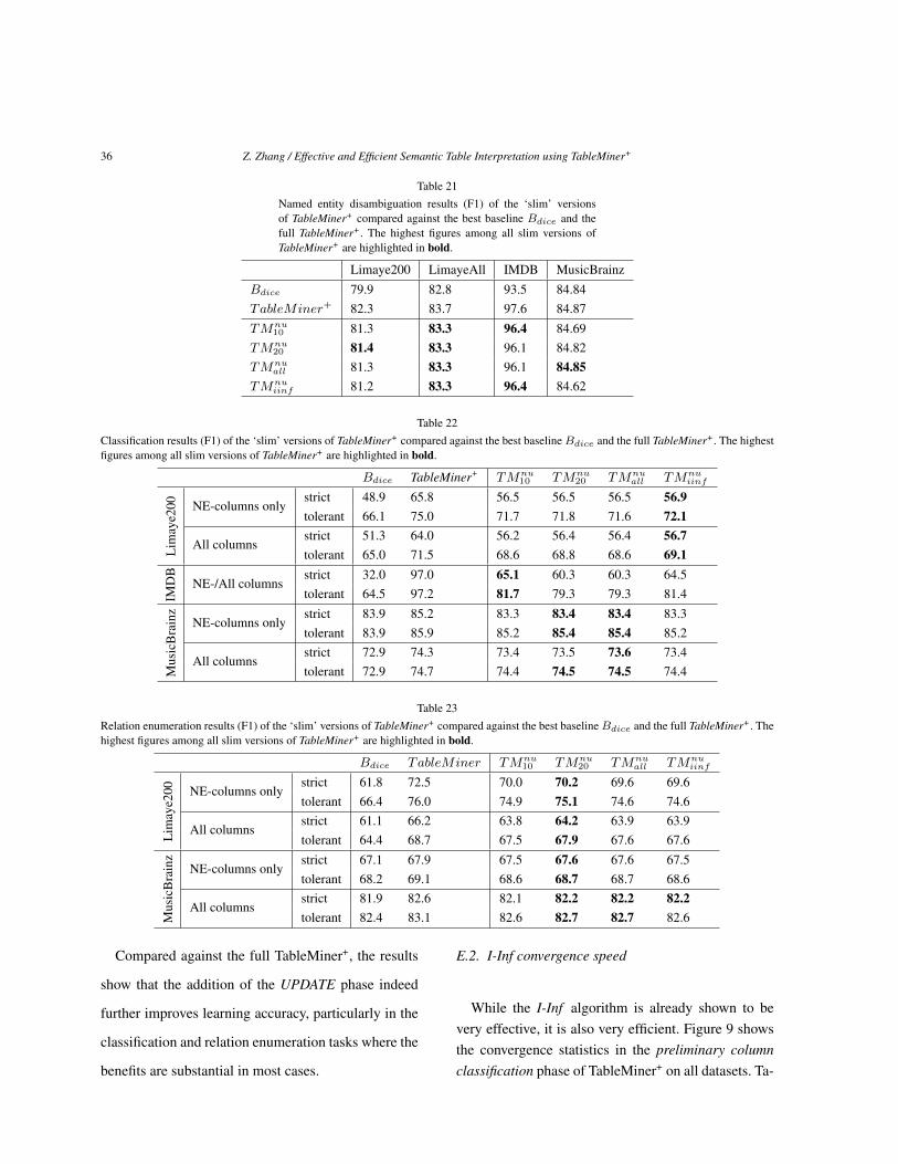
36 Z. Zhang / Effective and Efficient Semantic Table Interpretation using TableMiner+
Table 21Named entity disambiguation results (F1) of the ‘slim’ versionsof TableMiner+ compared against the best baseline Bdice and thefull TableMiner+. The highest figures among all slim versions ofTableMiner+ are highlighted in bold.
Limaye200 LimayeAll IMDB MusicBrainzBdice 79.9 82.8 93.5 84.84TableMiner+ 82.3 83.7 97.6 84.87TMnu
10 81.3 83.3 96.4 84.69TMnu
20 81.4 83.3 96.1 84.82TMnu
all 81.3 83.3 96.1 84.85TMnu
iinf 81.2 83.3 96.4 84.62
Table 22Classification results (F1) of the ‘slim’ versions of TableMiner+ compared against the best baseline Bdice and the full TableMiner+. The highestfigures among all slim versions of TableMiner+ are highlighted in bold.
Bdice TableMiner+ TMnu10 TMnu
20 TMnuall TMnu
iinf
Lim
aye2
00 NE-columns onlystrict 48.9 65.8 56.5 56.5 56.5 56.9tolerant 66.1 75.0 71.7 71.8 71.6 72.1
All columnsstrict 51.3 64.0 56.2 56.4 56.4 56.7tolerant 65.0 71.5 68.6 68.8 68.6 69.1
IMD
B
NE-/All columnsstrict 32.0 97.0 65.1 60.3 60.3 64.5tolerant 64.5 97.2 81.7 79.3 79.3 81.4
Mus
icB
rain
z
NE-columns onlystrict 83.9 85.2 83.3 83.4 83.4 83.3tolerant 83.9 85.9 85.2 85.4 85.4 85.2
All columnsstrict 72.9 74.3 73.4 73.5 73.6 73.4tolerant 72.9 74.7 74.4 74.5 74.5 74.4
Table 23Relation enumeration results (F1) of the ‘slim’ versions of TableMiner+ compared against the best baseline Bdice and the full TableMiner+. Thehighest figures among all slim versions of TableMiner+ are highlighted in bold.
Bdice TableMiner TMnu10 TMnu
20 TMnuall TMnu
iinf
Lim
aye2
00 NE-columns onlystrict 61.8 72.5 70.0 70.2 69.6 69.6tolerant 66.4 76.0 74.9 75.1 74.6 74.6
All columnsstrict 61.1 66.2 63.8 64.2 63.9 63.9tolerant 64.4 68.7 67.5 67.9 67.6 67.6
Mus
icB
rain
z
NE-columns onlystrict 67.1 67.9 67.5 67.6 67.6 67.5tolerant 68.2 69.1 68.6 68.7 68.7 68.6
All columnsstrict 81.9 82.6 82.1 82.2 82.2 82.2tolerant 82.4 83.1 82.6 82.7 82.7 82.6
Compared against the full TableMiner+, the results
show that the addition of the UPDATE phase indeed
further improves learning accuracy, particularly in the
classification and relation enumeration tasks where the
benefits are substantial in most cases.
E.2. I-Inf convergence speed
While the I-Inf algorithm is already shown to bevery effective, it is also very efficient. Figure 9 showsthe convergence statistics in the preliminary columnclassification phase of TableMiner+ on all datasets. Ta-

Z. Zhang / Effective and Efficient Semantic Table Interpretation using TableMiner+ 37
Fig. 9. Convergence statistics (max, min, average (black diamond),kth quantiles) for I-Inf at the LEARNING phase. itr - number ofiterations (rows processed) until convergence; % - fraction of contentcells processed in a column
Table 24Statistics of the slowest convergence of I-Inf when used for preliminarycolumn classification in the LEARNING phase.
Limaye200
LimayeAll
IMDB MusicBrainz
100% of rows processed in% of tables 33.8% 30.7% 27.6% 7.5%Avg. rows 11.0 10.0 13.0 8.5Rows >20 10 190 0 24
>50% of rows processed in% of tables 47.8% 47.6% 49.2% 13.9%Avg. rows 11.4 11.0 12.0 8.6Rows >20 16 442 0 47
ble 24 shows the statistics of the slowest convergenceon each dataset.
On all datasets, I-Inf in the preliminary column clas-sification phase typically converges in an average of 10iterations. In other words, only 10 cells are processedto create preliminary column classification. This alsoexplains the observation that the learning accuracy ob-tained by TMnu
iinf is very similar to TMnu10 . It repre-
sents about 55% of data in an average table from theLimaye200 and LimayeAll datasets, less than 30% inthe case of MusicBrainz, and about 75% for IMDBwhere the majority (75%) are small tables (see Figure7). In the cases that TableMiner+ does not converge orconverges slowly (Table 24), the tables are very small.
F. Mathematical notation lookup table
Continue on the next page.
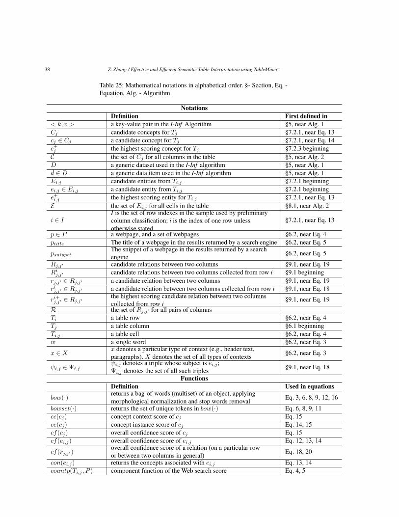
38 Z. Zhang / Effective and Efficient Semantic Table Interpretation using TableMiner+
Table 25: Mathematical notations in alphabetical order. §- Section, Eq. -Equation, Alg. - Algorithm
NotationsDefinition First defined in
< k, v > a key-value pair in the I-Inf Algorithm §5, near Alg. 1Cj candidate concepts for Tj §7.2.1, near Eq. 13cj ∈ Cj a candidate concept for Tj §7.2.1, near Eq. 14c+j the highest scoring concept for Tj §7.2.3 beginningC the set of Cj for all columns in the table §5, near Alg. 2D a generic dataset used in the I-Inf algorithm §5, near Alg. 1d ∈ D a generic data item used in the I-Inf algorithm §5, near Alg. 1Ei,j candidate entities from Ti,j §7.2.1 beginningei,j ∈ Ei,j a candidate entity from Ti,j §7.2.1 beginninge+i,j the highest scoring entity for Ti,j §7.2.1, near Eq. 13E the set of Ei,j for all cells in the table §8.1, near Alg. 2
i ∈ II is the set of row indexes in the sample used by preliminarycolumn classification; i is the index of one row unlessotherwise stated
§7.2.1, near Eq. 13
p ∈ P a webpage, and a set of webpages §6.2, near Eq. 4ptitle The title of a webpage in the results returned by a search engine §6.2, near Eq. 5
psnippetThe snippet of a webpage in the results returned by a searchengine §6.2, near Eq. 5
Rj,j′ candidate relations between two columns §9.1, near Eq. 19Rij,j′ candidate relations between two columns collected from row i §9.1 beginningrj,j′ ∈ Rj,j′ a candidate relation between two columns §9.1, near Eq. 19rij,j′ ∈ Rj,j′ a candidate relation between two columns collected from row i §9.1, near Eq. 18
ri+j,j′ ∈ Rj,j′the highest scoring candidate relation between two columnscollected from row i
§9.1, near Eq. 19
R the set of Rj,j′ for all pairs of columnsTi a table row §6.2, near Eq. 4Tj a table column §6.1 beginningTi,j a table cell §6.2, near Eq. 4w a single word §6.2, near Eq. 3
x ∈ X x denotes a particular type of context (e.g., header text,paragraphs). X denotes the set of all types of contexts §6.2, near Eq. 3
ψi,j ∈ Ψi,jψi,j denotes a triple whose subject is ei,j ;Ψi,j denotes the set of all such triples §9.1, near Eq. 18
FunctionsDefinition Used in equations
bow(·) returns a bag-of-words (multiset) of an object, applyingmorphological normalization and stop words removal Eq. 3, 6, 8, 9, 12, 16
bowset(·) returns the set of unique tokens in bow(·) Eq. 6, 8, 9, 11cc(cj) concept context score of cj Eq. 15ce(cj) concept instance score of cj Eq. 14, 15cf(cj) overall confidence score of cj Eq. 15cf(ei,j) overall confidence score of ei,j Eq. 12, 13, 14
cf(rj,j′)overall confidence score of a relation (on a particular rowor between two columns in general) Eq. 18, 20
con(ei,j) returns the concepts associated with ei,j Eq. 13, 14countp(Ti,j , P ) component function of the Web search score Eq. 4, 5
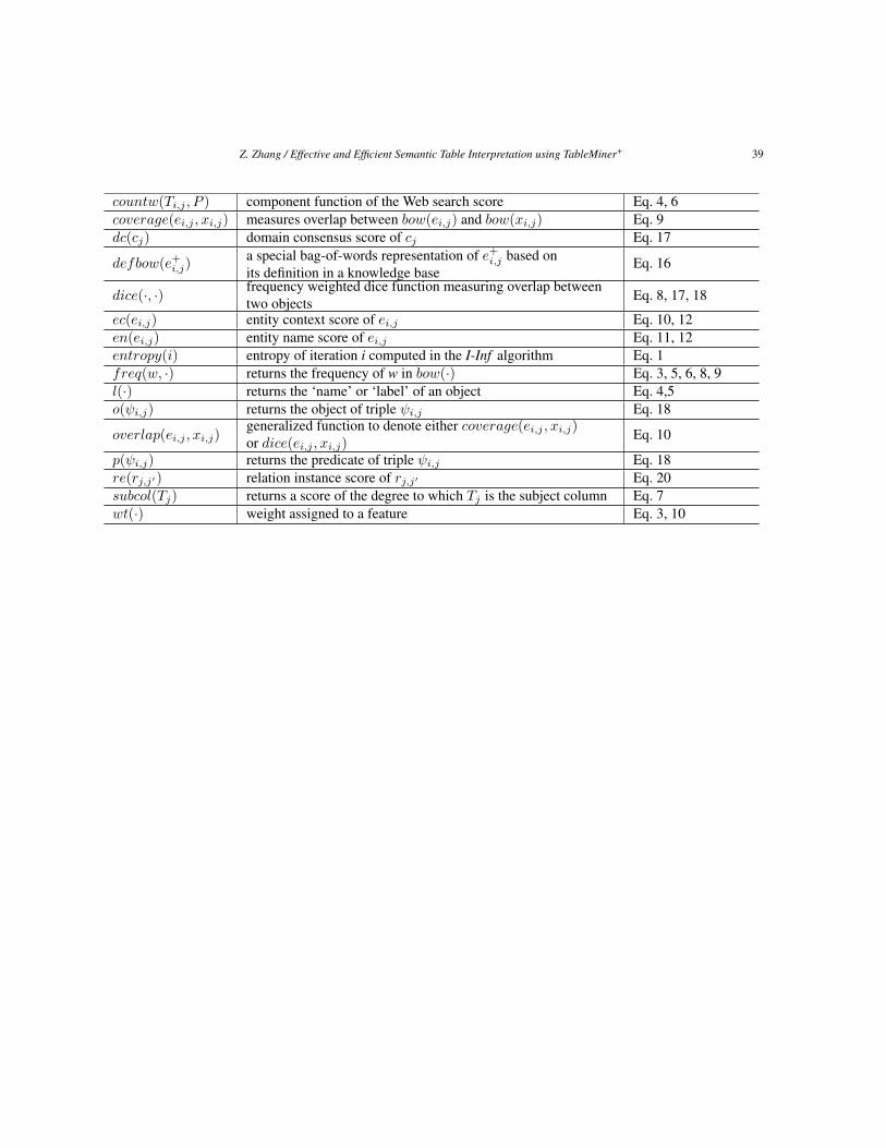
Z. Zhang / Effective and Efficient Semantic Table Interpretation using TableMiner+ 39
countw(Ti,j , P ) component function of the Web search score Eq. 4, 6coverage(ei,j , xi,j) measures overlap between bow(ei,j) and bow(xi,j) Eq. 9dc(cj) domain consensus score of cj Eq. 17
defbow(e+i,j)
a special bag-of-words representation of e+i,j based on
its definition in a knowledge baseEq. 16
dice(·, ·) frequency weighted dice function measuring overlap betweentwo objects Eq. 8, 17, 18
ec(ei,j) entity context score of ei,j Eq. 10, 12en(ei,j) entity name score of ei,j Eq. 11, 12entropy(i) entropy of iteration i computed in the I-Inf algorithm Eq. 1freq(w, ·) returns the frequency of w in bow(·) Eq. 3, 5, 6, 8, 9l(·) returns the ‘name’ or ‘label’ of an object Eq. 4,5o(ψi,j) returns the object of triple ψi,j Eq. 18
overlap(ei,j , xi,j)generalized function to denote either coverage(ei,j , xi,j)or dice(ei,j , xi,j)
Eq. 10
p(ψi,j) returns the predicate of triple ψi,j Eq. 18re(rj,j′) relation instance score of rj,j′ Eq. 20subcol(Tj) returns a score of the degree to which Tj is the subject column Eq. 7wt(·) weight assigned to a feature Eq. 3, 10