Embed Size (px)
Citation preview

Effect of wind modelling on simulation of passive ventilation
Boris Chernyavsky Hydrogen Safety Engineering and Research Centre (HySAFER)
http://hysafer.ulster.ac.uk/
HySafe Research Priorities Workshop Washington DC, 10-11 November 2014

Experimental conditions
Numerical simulations are compared against experiment WP2/25 performed by Health and Safety Laboratory (HSL) within HyIndoor project
"Accumulation of hydrogen released into an enclosure fitted with passive vents - experimental results and simple models" by Hooker P., Hoyes J.R., Hall, J., IChemE Hazards 24 Conference, 7-9 May 2014, Edinburgh, UK
Sonic release of hydrogen into an enclosure with single vent with initial tank pressure 17 bars with 169 Nl/min flow rate through 0.55 mm diameter nozzle. Release duration is 1400 seconds.
External wind with average velocity of 2.63 m/s.
Experiment WP2/25 exhibited least layering. Hydrogen concentration did not quite reached steady state maximum by the end of release.
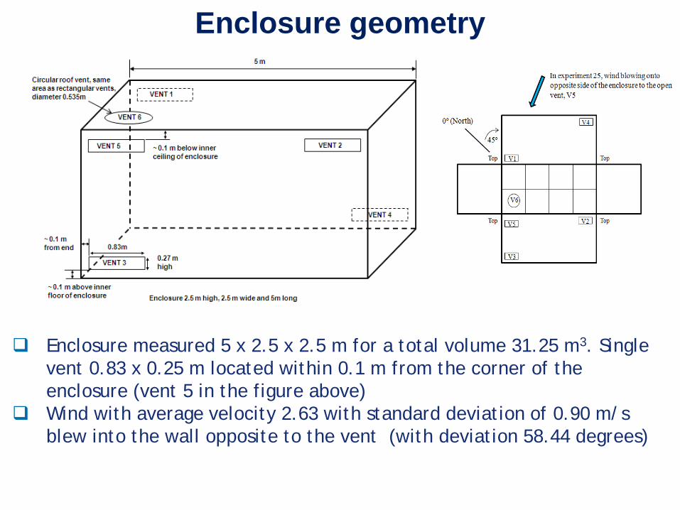
Enclosure geometry
Enclosure measured 5 x 2.5 x 2.5 m for a total volume 31.25 m3. Single vent 0.83 x 0.25 m located within 0.1 m from the corner of the enclosure (vent 5 in the figure above)
Wind with average velocity 2.63 with standard deviation of 0.90 m/s blew into the wall opposite to the vent (with deviation 58.44 degrees)
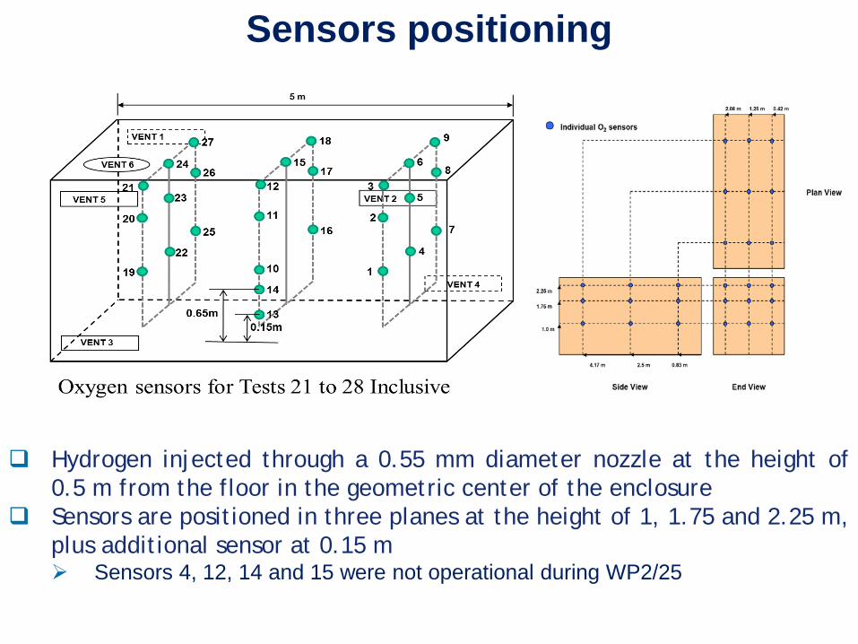
Sensors positioning
Hydrogen injected through a 0.55 mm diameter nozzle at the height of 0.5 m from the floor in the geometric center of the enclosure
Sensors are positioned in three planes at the height of 1, 1.75 and 2.25 m, plus additional sensor at 0.15 m Sensors 4, 12, 14 and 15 were not operational during WP2/25
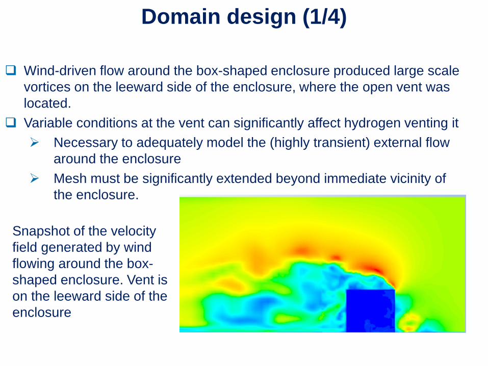
Domain design (1/4) Wind-driven flow around the box-shaped enclosure produced large scale
vortices on the leeward side of the enclosure, where the open vent was located.
Variable conditions at the vent can significantly affect hydrogen venting it Necessary to adequately model the (highly transient) external flow
around the enclosure Mesh must be significantly extended beyond immediate vicinity of
the enclosure.
Snapshot of the velocity field generated by wind flowing around the box-shaped enclosure. Vent is on the leeward side of the enclosure
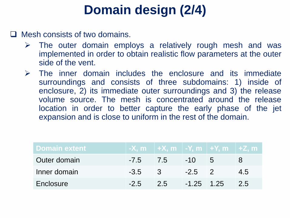
Domain design (2/4) Mesh consists of two domains. The outer domain employs a relatively rough mesh and was
implemented in order to obtain realistic flow parameters at the outer side of the vent.
The inner domain includes the enclosure and its immediate surroundings and consists of three subdomains: 1) inside of enclosure, 2) its immediate outer surroundings and 3) the release volume source. The mesh is concentrated around the release location in order to better capture the early phase of the jet expansion and is close to uniform in the rest of the domain.
Domain extent -X, m +X, m -Y, m +Y, m +Z, m Outer domain -7.5 7.5 -10 5 8 Inner domain -3.5 3 -2.5 2 4.5 Enclosure -2.5 2.5 -1.25 1.25 2.5
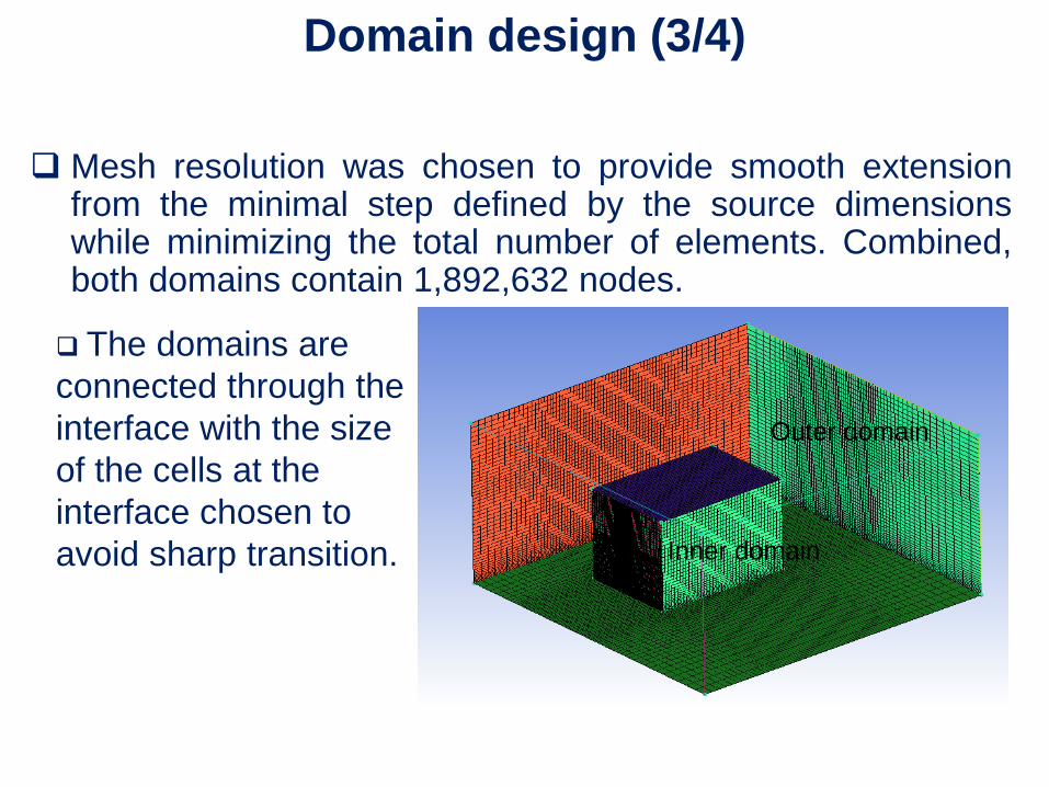
Domain design (3/4)
Mesh resolution was chosen to provide smooth extension from the minimal step defined by the source dimensions while minimizing the total number of elements. Combined, both domains contain 1,892,632 nodes.
The domains are connected through the interface with the size of the cells at the interface chosen to avoid sharp transition.
Outer domain
Inner domain
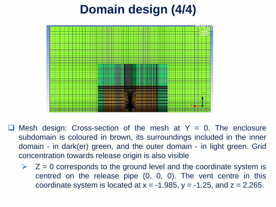
Domain design (4/4)
Mesh design: Cross-section of the mesh at Y = 0. The enclosure subdomain is coloured in brown, its surroundings included in the inner domain - in dark(er) green, and the outer domain - in light green. Grid concentration towards release origin is also visible Z = 0 corresponds to the ground level and the coordinate system is
centred on the release pipe (0, 0, 0). The vent centre in this coordinate system is located at x = -1.985, y = -1.25, and z = 2.265.
Numerical methodology
Numerical calculations were performed using ANSYS FLUENT (v.14.5) CFD simulation software.
A pressure based incompressible approach was used to solve the Navier-Stokes equation.
Turbulence closure was achieved by using the Large Eddy Simulation (LES) modelling technique with the Smagorinsky-Lilly subgrid scale (SGS) model.
Concentration was recorded at each timestep at the locations matching experimental sensor positions.
Simulation was allowed to run for ~ 80 seconds before starting hydrogen release in order to ensure correct flowfield at vent entrance
Hydrogen release continued for 1,400 seconds, after which simulation continued for approximately another 2,300 seconds in order to model hydrogen escape
Sonic release was modelled using volumetric source methodology
Volumetric source method (1/4) Volume source method had been developed to address two main
type of problems:
Simulation of release under high pressure
Simulation of blowdown
Two main features:
Utilizes distributed volume source
Utilizes Abel-Nobel equation of state for notional nozzle calculation
Originally published in:
V. Molkov, D. Makarov, and M. Bragin, Physics and modeling of under-expanded jets and hydrogen dispersion in atmosphere, Proceedings of the XXIV International Conference on Interaction of Intense Energy Fluxes with Matter, March 1-6 2009, Elbrus, Russia
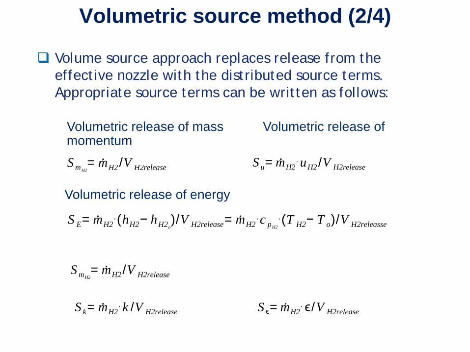
Volumetric source method (2/4) Volume source approach replaces release from the
effective nozzle with the distributed source terms. Appropriate source terms can be written as follows:
Volumetric release of mass Volumetric release of momentum
Volumetric release of energy
S mH2= mH2 /V H2release S u= mH2⋅uH2 /V H2release
S E= mH2⋅(hH2− hH2o)/V H2release= mH2⋅c pH2
⋅(T H2− T o)/V H2releasse
S mH2= mH2 /V H2release
S k= mH2⋅k /V H2release S ϵ= mH2⋅ϵ/V H2release

Volumetric source method (3/4) Previous studies indicated that volume source approach
provide accurate results with volume source dimensions up to 4 effective diameters
Validation based on comparison with HSL experiment (Roberts 2006) for P=100 bar quasi-steady release through 3 mm nozzle

Volumetric source method (4/4) Flow is effectively incompressible Relaxed numerical constrains Fester convergence Present simulation uses cube-shaped volume source with
the height and diameter of four effective diameters as calculated by Abel-Nobel equation, with four cells in each direction
Source region size Jet velocity Mach number 1 Deff 1032 m/s 0.87
2 Deff 415 m/s 0.46
4 Deff 164 m/s 0.28
8 Deff 72 m/s 0.15
Numerical results (1/5)
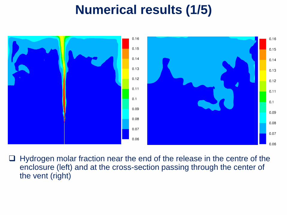
Hydrogen molar fraction near the end of the release in the centre of the
enclosure (left) and at the cross-section passing through the center of the vent (right)

Numerical results (2/5)
Hydrogen molar fraction in the vent cross-
section (left) Hydrogen concentration contours in the
release cross-section (right) Isoline plot of hydrogen concentration
field in the vent cross-section (bottom right)
Numerical results (3/5)
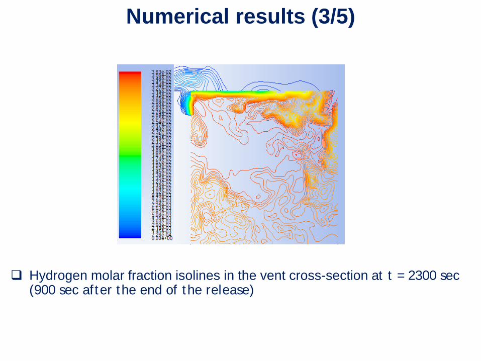
Hydrogen molar fraction isolines in the vent cross-section at t = 2300 sec
(900 sec after the end of the release)

Numerical results (4/5)
Comparison of time evolution of LES results and experimental
measurements of H2 concentrations at various heights
Numerical results (5/5)
Numerical results show good agreement with the experiment for maximum concentration level reached in the experiment (within ~2.5 %) and the shape of concentration rise curve
Numerical simulation produces higher stratification compared with experiment
Large oscillations in wind direction and vortices resulting from flow around rectangular body result in a highly unsteady conditions outside the vent
Numerical simulation is highly sensitive to the wind conditions, including vortical flows produced by flow around rectangular enclosure and turbulence levels set in the external domain Simulation with low turbulence levels in external domain
and/or with insufficient external domain extent to model vortical flow around the enclosure produced significant overestimate of hydrogen concentration inside the enclosure

Velocity field inside box
Initial velocity profiles in the vent cross-section (left) and in
the hydrogen pipe cross-section (right) prior to release start Artificial excitation of air inside the box before release did
not significantly affected concentration evolution

Wind effect (1/3)
The presence of the wind had significant effect on the mixture escape from the enclosure
In the experiment, the wind was observed to change both velocity and direction in a wide range
Simulation with a constant wind set at the external domain boundary with parameters corresponding to the average values produced significant over-prediction of the hydrogen concentration inside the enclosure
Results of the simulation with constant wind parameters resembled results of the simulation without taking into account wind effect
In order to simulate significant variations in wind direction and velocity, an artificial turbulence conditions were implemented at the external boundary Turbulence intensity on the outer boundary was set at 90% and
the turbulence length scale at 25 m, corresponding to the simulation scale
Artificial turbulence was used to mimic variation in wind parameters. Implementation of variable outer boundary conditions dramatically
improved agreement between simulation and experimentally observed results
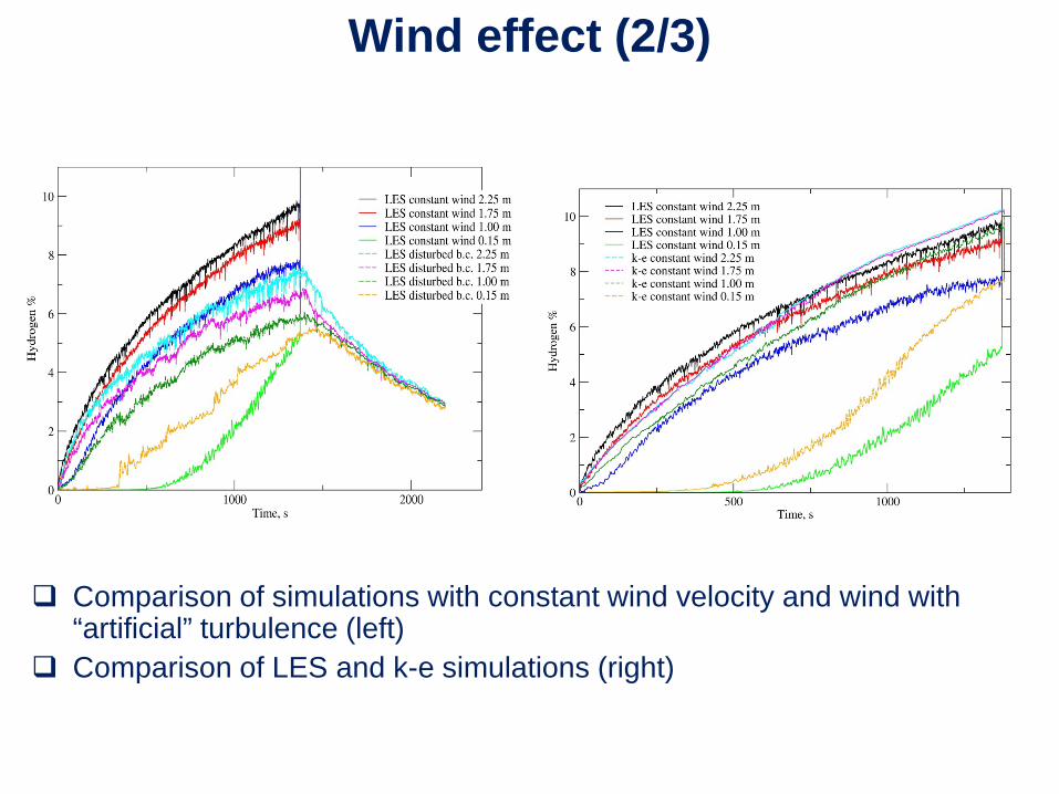
Wind effect (2/3)
Comparison of simulations with constant wind velocity and wind with
“artificial” turbulence (left) Comparison of LES and k-e simulations (right)

Wind effect (3/3)
Comparison of hydrogen concentration contours in the vent cross-section
for the case with constant wind (left) and wind with “artificial” turbulence (right)
Possible explanation for significant impact of wind variation is the destabilizing effect of variable wind on the flow condition near vent outlet. Variable wind prevent formation of the stationary vortex formed by flow around the box (with vent located high on the leeward side of the enclosure), which reduces outflow from the vent and decreases venting efficiency.

Acknowledgements: Fuel Cell and Hydrogen Joint Undertaking for support
through HyIndoor project and EC for funding of H2FC project
Health and Safety Executive for provision of experimental data


![ENERGY MODELLING AND PASSIVE DESIGN [2.2] Submittal Form](https://img.dokumen.tips/doc/110x75/6169e40111a7b741a34c8125/energy-modelling-and-passive-design-22-submittal-form.jpg)


