Effect of the Detector Dead-time Uncertainty on the

ANALYTICAL SCIENCES SEPTEMBER 2014, VOL. 30 871

Introduction

Isotope dilution mass spectrometry (IDMS) is a primary method of measurements suitable for the analysis of trace metals in inorganic materials. Though thermal ionization mass spectrometry has historically been used for a mass spectrometry device, inductively coupled plasma mass spectrometry (ICP-MS) has now become a leading method because of the high sensitivity and ability for multi-elemental analysis. In IDMS, the weighing of samples and enriched spike materials and measuring of the molar ratio of the analyte isotopes in the sample-spike mixture lead directly to analytical results. This is the reason why IDMS can be regarded as being one of primary methods. However, strictly speaking, the IDMS procedure is not traceable to the International System of Units (SI), unless the concentration of the spike is precisely determined by IDMS with an assay standard whose concentration is determined by a primary method such as gravimetry and colometric titration.1 Such a procedure in IDMS is called “reverse IDMS”. Simultaneous procedures of IDMS and reverse IDMS (“double

IDMS”) satisfy indispensable conditions for primary methods.Since an IDMS equation is expressed as a function of some

independent variables, an uncertainty statement for the analytical result can be simply written down by differentiating the equation. The parameters affecting a combined standard uncertainty of the analytical result include (a) the uncertainty of the concentration of the assay standard used for reverse IDMS, (b) the uncertainty of the isotopic composition of element in the sample and the assay standard, (c) the repeatability of the concentrations for IDMS mixtures and that for reverse IDMS mixtures, and (d) the precision and trueness of the isotope ratio measurement. Among the parameters, the most important one is the precision and the trueness of isotope ratio measurements.

As for the precision, the use of an ICP-sector field mass spectrometer operated in the low-resolution mode can produce more stable ion transmission and a lower background, resulting in better precision of the isotope ratio measurement close to the statistically limiting value.2–5 However, isotope ratio measurements in the medium-resolution mode suffer from a severer fluctuation problem in the peak top of the mass spectra, because the peak width of the spectra is in the range of several 10–3 amu. This may cause a severer effect on the precision of the isotope ratio measurement.6–11 Therefore, in the present study, a measurement procedure for the analysis of elements

2014 © The Japan Society for Analytical Chemistry

† To whom correspondence should be addressed.E-mail: [email protected]

Effect of the Detector Dead-time Uncertainty on the Analytical Result of Minor Elements in Low-alloy Steel by Isotope Dilution/ICP Sector Field Mass Spectrometry

Naoko NONOSE,† Akiharu HIOKI, and Koichi CHIBA

National Metrology Institute of Japan, National Institute of Advanced Industrial Science and Technology, 1-1-1 Umezono, Tsukuba, Ibaraki 305–8563, Japan

In the present study the effects of the detector dead-time and its uncertainties on the accuracy and uncertainty of isotope dilution mass spectrometry (IDMS) were considered through an interlaboratory study on the analysis of low-alloy steel by using an ICP-sector field mass spectrometer. Also, an optimized mixing ratio of the sample and the spike to obtain highly precise results was theoretically and experimentally investigated. The detector dead-time used in the interlaboratory study showed a negative value. However, it less affected the trueness of the analytical result if the dead-time correction for the measured isotope ratio was done properly. As many researchers have pointed out, the detector dead-time showed a clear mass dependence. Therefore, it is desirable to check the dead-time in every target element by using assay standards or isotopic standards, which would lead to an accurate result even if the detector dead-time is a negative value. On the other hand, the effect of the uncertainty of the detector dead-time can be minimized when both isotope ratios and ICP-MS signals of the [sample + spike] blend in IDMS are equal to those of [spike + assay standard] in reverse IDMS. From standpoints of error magnification theory and the precision of the isotope ratio measurement, an optimized isotope ratio of the sample-spike blend would be 1.0 for an element with a large difference in ten times and more between the atomic fractions of two isotopes used for IDMS. In the case of an element with no significant difference between the atomic fractions of two isotopes, an optimized isotope ratio can be calculated by a formula expressed as a function of the atomic fractions of the sample and the spike as well as the signal of ICP-MS.

Keywords IDMS in a medium-resolution mode, CCQM interlaboratory study, low-alloy steel, negative dead-time of the detector, uncertainty calculation

(Received April 4, 2014; Accepted July 29, 2014; Published September 10, 2014)

872 ANALYTICAL SCIENCES SEPTEMBER 2014, VOL. 30

requiring a medium-resolution mode of mass spectrometer was improved to attain a higher precision of the isotope ratio. Also, an optimized mixing ratio of the sample and the spike to obtain highly precise results was theoretically and experimentally investigated.

On the other hand, the trueness of the isotope ratio is greatly affected by (a) a mass discrimination appearing in a mass spectrometer12–14 and (b) the dead-time of an ion counting detector.12–18 When actual signals of ICP-MS exceed 100000 counts per second (cps) and in addition there is a large difference between the signals of two isotopes monitored, the effect of the detector dead-time becomes severer. The isotope ratio measurement at larger signals is preferable for higher precision; therefore, a precise correction of the effect by the detector dead-time is necessary. Accurate analytical results depend on the accuracy of the detector dead-time correction.

National Metrology Institute of Japan (NMIJ) has participated in various interlaboratory studies on trace metal impurities in inorganic materials organized by the Inorganic Analysis Working Group of the Consultative Committee for Amount of Substance-metrology in chemistry (CCQM),19 for example “Pb in water” and the “chemical composition in clay”. The CCQM is one of the consultative committees of the Bureau International des Poids et Mesures (BIPM). One of the roles of the CCQM is to ensure a worldwide uniformity (comparability) of measurements and the traceability to SI.20 The aim of our participations in the CCQM interlaboratory studies is not only to contribute to the international comparability of measurements, but also to demonstrate an analytical capability to produce reference materials as members of national metrology institutes in the world. In the present study, referring to an example of a CCQM interlaboratory study where trace metals including Cr, Ni and Mo in low-alloy steel were determined by IDMS coupled with ICP-sector field mass spectrometer, the effects of the detector dead-time and its uncertainty on the analytical result is discussed. Since two detectors employed in this experiment possessed different dead-times from each other, one showed a positive value and the other a negative value, the effect of the difference between the detectors on the accuracy of the analytical results and then the mass dependency of detector dead-time was also discussed.

Experimental

In this paper since many symbols appear in the text and formulas, explanations for these symbols are summarized in Table 1.

InstrumentationThe double-focusing sector-field inductively coupled plasma

mass spectrometer (ICP-SFMS) used in the present study was an Element 2 (Thermo Fisher Scientific Inc., Bremen, Germany), equipped with a PFA nebulizer with sample uptake rate of 100 μL min–1 and a double pass–glass spray chamber developed for stable isotope ratio measurements. In this instrument, transmitted ions strike a conversion dynode, and then electrons ejected from it are detected by a secondary electron multiplier equipped with discrete dynodes (SEM). The mass spectrometer was operated in a low-resolution mode (m/Δm = 400) for the determination of Ni and Mo, free from spectral interferences, and operated in a medium-resolution mode (m/Δm = 4000) in the determination of Cr in order to prevent spectral interferences caused by 40Ar12C+, 35Cl16O+ and 37Cl16O+. The typical operating conditions of the ICP and data-acquisition parameter for isotope

ratio measurements are listed in Table 2. For the digestion of low-alloy steel, a microwave digester ETHOS PLUS (Milestone, Socisole, Italy) with 10 high-pressure PTFE vessels was employed.

Outline of interlaboratory studyThe CCQM interlaboratory study in which we participated

involved the determination of minor elements (Cr, Ni, Mn and Mo) in low-alloy steel. The NMIJ was one of the pilot laboratories responsible for this interlaboratory study, preparing and distributing sample materials to participants and reporting the results. Thirty grams of the low-alloy steel tips were in each sample bottle. The mass fraction levels for analyte elements were in the range from 0.4 to 2%. Other than the analyte

Table 1　List of symbols used in the text and formulas

Nt number of incident ions per one secondNo number of actually observed ions per one secondτo, τ dead-time of secondary electron multiplier with

discrete dynodeP isotope ratio corrected with a tentative value of

detector dead-time τIA measured signals of ICP-MS for mass A or measured

signals of IDMS for mass AIB measured signals of ICP-MS for mass B or measured

signals of IDMS for mass BRt (IS(1)) true isotope ratio for [Isotope standard](run1)Ro (IS(1)) measured isotope ratio for [Isotope standard](run1)K1 correction factor for [Isotope standard](run1)

expressed as Rt (IS(1))/Ro (IS(1))K2 correction factor for [Isotope standard](run2)

expressed as Rt (IS(2))/Ro (IS(2))K(b-sam1) correction factor for measured isotope ratio of [blend

sam1]Rc (b-sam1) corrected isotope ratio for measured isotope ratio of

[blend sam1]Cx concentration of sample in mol kg–1 unitCy concentration of spike in mol kg–1 unitCz concentration of assay standard in mol kg–1 unitKbl correction factor for blend of sample and spikeKbl′ correction factor for blend of spike and assay standardAf (massA, x) atomic fraction of mass A in samplea atomic fraction of mass A in assay standardb atomic fraction of mass B in assay standardR′ corrected isotope ratio for blend of spike and assay

standard expressed as Kbl′Rbl′

c atomic fraction of mass A in spiked atomic fraction of mass B in spikeα (a – R′b)/(R′d – c)R corrected isotope ratio for blend of sample and spike

expressed as KblRbl

e atomic fraction of mass A in samplef atomic fraction of mass B in sampleβ (Rd – c)/(e – Rf)Il smaller signal of ICP-MS in isotope ratio measurementIh larger signal of ICP-MS in isotope ratio measurementR(1) optimized isotope ratios calculated considering

uncertainty of IDMSR(2) optimized isotope ratios calculated from error

magnification factorR(τ) dead-time corrected isotope ratio expressed as

IA(1 – τIB)/IB(1 – τIA) in IDMSI′A measured signals of reverse IDMS for mass AI′B measured signals of reverse IDMS for mass BR′ (τ) dead-time corrected isotope ratio expressed as

I′A(1 – τI′B)/I′B(1 – τI′A) in reverse IDMSγ {(R(τ)d – c)/(e – R(τ)f)}{(a – R′ (τ)b)/(R′ (τ)d – c)


elements, C, Si, Cu and V were also included in the range from 0.1 to 0.5%. While participants including the CCQM members were welcome to use any method of measurement, we employed the IDMS method, regarded as being a possible one of the primary methods of measurement by CCQM,1,20 for determining Cr, Ni, and Mo. Manganese was determined by both an ICP optical emission spectrometry and ICP-MS coupled with a matrix matched calibration method. Details of the analytical results for Mn, however, were not reported in the present study.

Chemicals and reagentsNickel, Mo and Cr stock standard solutions of 1000 mg kg–1

were gravimetrically prepared by dissolving high-purity materials: Ni in metallic form (99.99% purity), Mo in metallic form (99.99% purity), and Cr in form of K2Cr2O7 (99.99% purity), respectively. For each element, two independent stock solutions, Assay1 and Assay2, were prepared to confirm whether the preparation procedure including the dilution of stock solutions and the spike and assay standard mixture was exactly performed.

The standard uncertainties of the concentration for these solutions were estimated to be 0.5 mg kg–1. Each stock solution was stored in polyethylene containers with a middle cap in a top cap. These stock solutions were further diluted gravimetrically with 0.3 mol dm–3 HNO3 to desired concentrations.

Enriched spike materials used in the present study were 61Ni in the metallic form, 100Mo in the metallic form and 53Cr in the oxide form (Cr2O3), purchased from Oak Ridge National Laboratory (Oak Ridge, TN). The isotopic compositions for these spikes are listed in Table 3. While both the 61Ni spike solution and the 100Mo spike one were prepared by dissolving corresponding material in 1 mol dm–3 HNO3, the 53Cr spike material was dissolved in a sodium bromate maturated solution kept at 150°C. Other reagents used for sample preparation, such as nitric acid, hydrochloric acid and highly purified water, were of ultra-pure grade (Kanto Chemicals Co., Inc., Tokyo, Japan). Polypropylene containers were used throughout the solution preparation required for the IDMS analysis.

Preparation of spike mixed solutions for IDMS and reverse IDMSWhether an accurate analysis is achieved by the IDMS method

partly depends on the selection of the optimum mixing ratio of the spike and the sample. According to the protocol of the IDMS method proposed by NIST21 and the result of our previous experiment,22 the amount of spike aliquot mixed with the sample in IDMS, and that mixed with the assay standard in reverse IDMS were decided. It is needless to say that accurate weighing of the sample materials and solutions is necessary to ensure traceability to the SI; on the other hand, we do not need to know accurate dilution factors of the mixed solutions. In the present study all samples were weighed accurately with a sensitivity of 10 μg in order to omit any uncertainty due to the weighing of materials from a calculation of the uncertainty budget for the analytical result.

Sample-spike blends for IDMSAbout 0.5 g of low-alloy steel tips were weighed into a PFA

vessel, and then 20 mL of 6 mol dm–3 HNO3 was added to the vessel. After tightly capping six vessels (four samples and two reagent blanks), the vessels were placed in the microwave digester. Two steps of heating started: heating from 20 to 190°C for 15 min and heating kept at 190°C for 20 min. After cooling, each dissolved sample was diluted to 50 g with 0.3 mol dm–3 HNO3. About 2.0 g of a 130 mg kg–1 53Cr enriched spike solution, about 5.0 of a 100 mg kg–1 61Ni enriched one and about 1.0 g of a 200 mg kg–1 100Mo enriched one were mixed with a 10 g portion of the diluted sample solution in a polypropylene container, and then the mixed solution was diluted to about 100 g with 0.3 mol dm–3 HNO3. Four sample-spike blends were termed [Spike+Sam1], [Spike+Sam2], [Spike+Sam3], and [Spike+Sam4]. In the same manner as the sample-spike blends, two blank-spike blends were prepared by adding a 10-fold diluted spike solution (Spikedil) to each sample. These blends were termed [Spikedil+Blk1] and [Spikedil+Blk2].

It is desirable that a spike aliquot is added to the sample before the digestion procedure or before any dilution process so as to avoid any unexpected loss of the analyte during a sample digestion procedure. However, in the present study, a spike aliquot was mixed with a 5-fold quantitatively diluted solution of the dissolved sample, because the concentration levels of the analytes in low-alloy steel are far higher than those of spike stock solutions.

Table 2　Operating conditions of ICP–mass spectrometer and acquisition parameters for isotope ratio measurements

ICP operating conditions Rf power/W Carrier gas/L min–1

Aux. gas/L min–1

Plasma gas/L min–1

Sampling depth/mm

14501.050.83154.3

Isotope ratio measurement Resolution of mass spectrometer (m/Δm) Dwell time/ms Settling time/ms Mass window

Sampling points

Number of sweeps

Accumulation

4000 for Cr400 for Ni and Mo213% for correction of maximum peak position

150% for profile check solution3 for isotope ratio measurement60 for profile check solution600 for isotope ratio measurement10 for profile check solution10 for isotope ratio measurement5 for profile check solution

Table 3　Isotopic composition of Cr, Ni and Mo spikes

Element Isotopic compositiona

Cr 50Cr: 0.00030 ± 0.0000552Cr: 0.0265 ± 0.000253Cr: 0.9720 ± 0.000254Cr: 0.0012 ± 0.00005

Ni 58Ni: 0.0013 ± 0.000160Ni: 0.0019 ± 0.000161Ni: 0.9944 ± 0.000262Ni: 0.0005 ± 0.000164Ni: 0.0019 ± 0.0001

Mo 92Mo: 0.0033 ± 0.000494Mo: 0.0009 ± 0.000295Mo: 0.0015 ± 0.000396Mo: 0.0038 ± 0.000597Mo: 0.0012 ± 0.000298Mo: 0.0034 ± 0.0005100Mo: 0.9859 ± 0.0017

a. All are vendor values.


Spike-assay blends for reverse IDMSIn parallel with the preparation of sample-spike blends,

spike-assay standard blends were also prepared. Such a parallel procedure can compensate for the effect of any uncertainty due to the isotopic composition of the spike on the final result. About 1.0 g of a 100 mg kg–1 Cr standard solution was added to about 1.0 g of a 130 mg kg–1 53Cr enriched spike solution. In the same way, about 0.4 g of a 1000 mg kg–1 Ni standard solution was mixed with about 1.0 g of a 100 mg kg–1 61Ni enriched spike solution, and about 1.0 g of a 1000 mg kg–1 Mo standard solution was mixed with about 1.0 g of a 200 mg kg–1 100Mo enriched spike solution. For each element, two spike-assay standard blends [Spike+Assay1], [Spike+Assay2] were prepared.

The dilution factor for each spike-mixed solution was decided to yield a signal of ICP-MS in the range from 800000 to 1000000 cps for the major isotope, which corresponds to about 10 μg kg–1 of Cr, measured in the medium-resolution mode, and about 3 μg kg–1 of Mo and Ni, measured in the low-resolution mode.

Isotope ratio measurement by ICP-SFMSThe isotope pairs to be measured were 52Cr/53Cr, 60Ni/61Ni, and

95Mo/100Mo. As mentioned in the instrumentation section, the sector field mass spectrometer was operated in a medium-resolution mode (m/Δm = 4000) for Cr, and in a low-resolution mode (m/Δm = 400) for Ni and Mo, using the electrostatic scanning mode. The acquisition parameters for isotope ratio measurements are listed in Table 2. In order to obtain precise isotope ratios, several parameters including the number of scans, dwell time, points per peak, and mass window were optimized for both resolution modes.

The measurement order of the solutions prepared for reverse IDMS of Cr was; (1) [Assay standard] (correction of the maximum peak position in the mass table), (2) [Assay standard] (correction of mass discrimination), (3) [Spike+Assay1], (4) [Spike+Assay2], (5) [Assay standard] (correction of mass discrimination), (6) 1 mol dm–3 HNO3 (washing the sample introduction system of the ICP-mass spectrometer). Hereafter, “Spike+Assay1” was used as a “Working solution” for a mass discrimination correction in the IDMS measurement.

The measurement order of solutions prepared for IDMS of Cr (run1) was: (1) [Profile check solution] (correction of the

Fig. 1　Measurement procedure of IDMS samples, isotopic standards and profile check solutions for corrections of the mass discrimination and maximum peak position.


maximum peak position in the mass table), (2) [Working solution] (correction of the mass discrimination), (3) [Spike+Sam1], (4) [Spike+Sam2], (5) [Working solution], (6) [Spike+Sam3], (7) [Spike+Sam4], (8) [Working solution], (9) [Spikedil+Blk1], (10) [Spikedil+Blk2], (11) [Working solution], (12) 1 mol dm–3 HNO3. In the second run (run2), four sample-spike blends were measured in the reverse order. Double correction procedures of the maximum peak position and the mass discrimination are necessary to obtain good precision of the isotope ratio measurements, especially in the medium-resolution mode. Details of these correction methods are discussed later. In the cases of Ni and Mo, however, a correction of the maximum peak in the mass table is not necessary. The measurement order of IDMS samples, isotopic standards and profile check solutions is shown in Fig. 1.

Results and Discussion

Double correction procedures for maximum peak position and mass discrimination in the medium-resolution mode of ICP-SFMS

In ICP-SFMS, the flat-top peak shape obtained in the low-resolution mode allows for a higher precision of isotope ratio measurements, probably because of stable ion transmission in the sector field mass spectrometer, and its lower background level. Despite inevitable fluctuation effects of the ICP and the sample introduction system, the relative standard deviation (RSD) for 10 replicate measurements of isotope ratios obtained by ICP-SFMS in the low-resolution mode was by a factor of 2 – 5 superior to that obtained by the ICP-quadrupole mass spectrometer.

On the other hand, a peak shape obtained in the medium-resolution mode has a non-flat top (Fig. 2(A)). Therefore, the peak top would be more subject to the fluctuation effect of the mass analyzer than the flat-top peak in the low-resolution mode.

Fig. 2　Peak shapes observed in IDMS measurements at medium-resolution mode.(A) For correction of maximum peak position, 150% peak integration window was applied. (B) For isotope ratio measurements, only 3% peak integration window was applied.(C) Peak top after several measurements was shifted from the true mass.


In addition, the peak position in the medium-resolution mode drifts with the measurement time (Fig. 2(C)) in the range of sub-milli amu (~ 0.0005). Usually, the isotope ratio measurement requires a correction of the mass discrimination effect using isotopic standard solutions or appropriate working solutions whose isotopic ratios are calibrated. In the present study, such working solutions were measured for every two or four sample solutions in order to control the influence of the time-drift of the mass discrimination, irrespective of the resolution of the mass spectrometer. However, isotope ratio measurements in the medium-resolution mode require an additional correction of the “maximum peak position” in the mass table, which means “Mass offset and Lock mass” in the operation software of Element2. This software corrects for any difference between the “maximum peak position” in the mass table yielding the peak top and “true mass” automatically. However, even with this software for automatic mass shift correction, the drift of peak top position in a sub-milli amu range could not be entirely corrected. Therefore the correction of the “maximum peak position” was done using a “profile check solution” at a regular interval in the IDMS measurement sequence.

In correcting for mass discrimination as well as the isotope ratio measurement, three points around the peak top, corresponding to a 2 – 3% peak integration window, are measured (Fig. 2(B)) in order to obtain high precision. In the correction of the “maximum peak position”, sixty points per isotope, corresponding to 150% of the peak integration window, are measured to check the peak shape (Fig. 2(A)). After several measurements of spike+sample blend solutions, the peak top is shifted from the “true mass”. Thus, the difference between the “maximum peak position” in the mass table yielding the peak top and “true mass” is corrected by measuring the profile check solution again. As a result of the double correction procedure, 0.2% or less precision of the isotope ratio measurement (n = 10, total acquisition time of 150 s) was attained. This precision was almost the same as that obtained in the low-resolution mode, yielding a flat top peak (0.05 – 0.1%).

Correction of measured isotope ratioIn our isotope ratio measurements the isotopic standard

solution was measured every two sample-spike blend in IDMS or every two spike-assay blends in reverse IDMS to correct for both the mass discrimination and the time-drift of the mass spectrometer; [Isotope standard](run1) → [blend sam1] → [blend sam2] → [Isotope standard](run2)

The correction factors for [Isotope standard](run1) and [Isotope standard](run2) are termed K1 and K2, respectively. The K1 and K2 values are defined as

K RR

K RR

1 ISIS

ISIS

t

o

t

o

= =( ( ))( ( ))

( ( ))( ( ))

.11

2 22 (1)

Here, Rt(IS(1)) means the true isotope ratio for [Isotope standard](run1), and Ro(IS(1)) means the measured isotope ratio for [Isotope standard](run1) after a correction for the detector dead-time(τ0).

RI

Io

o

o o

ISIS massA

IS mass( ( ))

( ( ), )( ( ),

11

1 1=

− ⋅τ AAIS massB

IS massBo o

o)( ( ), )

( ( ), ).⋅ − ⋅1 1

1τ II (2)

Here, Io(IS(1), massA) and Io(IS(1), massB) are the signals at massA and massB of the sample solution [Isotope standard](run1), respectively.

Correction factors for the measured isotope ratios of [blend sam1] and [blend sam2], defined as K(b-sam1) and K(b-sam2),

respectively, are calculated considering time-drift effect of mass discrimination as follows:

KK K

KK K

( ) , ( ) .b-sam1 b-sam2= ⋅ + = + ⋅2 1 23

1 2 23

(3)

In general, because the correction factors change linearly with the measurement time, both the K(b-sam1) and K(b-sam2) values were calculated from the weighted mean of K1 and K2. Corrected isotope ratios for the measured isotope ratios of [blend sam1] and [blend sam2], termed Rc(b-sam1) and Rc(b-sam2), are calculated:

R k R

R

c o

c

b-sam1 b-sam1 b-sam1

b-sam2

( ) ( ) ( ),

( )

= ⋅= kk R( ) ( ).b-sam2 b-sam2o⋅

(4)

Here, Ro(b-sam1) and Ro(b-sam2) mean the measured isotope ratio for [blend sam1] and [blend sam2] after a correction of the detector dead-time (τ0) with Eq. (2).

Calculation of the analytical resultsThe mass fraction of the elements in the sample can be

calculated according to the IDMS equation (Eq. (5)) and reverse IDMS equation (Eq. (6)) proposed by NIST.21

C Cmm

K R A y A yAx y

y

x

bl bl f fmassB, massA,= ⋅ ⋅ ⋅ ⋅ −( ) ( )ff bl bl fmassA, massB,( ) ( )

,x K R A x− ⋅ ⋅ (5)

C C mm

A z K R Ay z

z

y

f bl bl fmassA, massB,= ⋅′⋅ − ⋅ ⋅′ ′( ) ( zzK R A y A y

)( ) ( )

.bl bl f fmassB, massA,′ ′⋅ ⋅ − (6)

Here, subscripts x, y, z, bl and bl′ indicate the sample, spike, assay standard, blend of sample and spike, blend of spike and assay standard, respectively. C indicates the concentration in mol kg–1 unit, m, mass in kg unit, R, measured isotope ratio after a correction of the detector dead-time, K, correction factor for the measured isotope ratio, and Af , atomic faction. For example, Af (massA, x) is the atomic fraction of mass A in the sample. In this IDMS calculation, isotopic composition data used were from Isotopic Compositions of the Elements 2009.23

As can be easily seen in Eqs. (5) and (6), all the variables involved in calculating the spike concentration and the sample concentration are independent variables. The uncertainty of the sample concentration (Cx) can be evaluated by combining the standard uncertainties of all the variables, following the uncertainty propagation law for independent variables, xi, to a function f in the JCGM 100:2008,24

u ffx

u x2

2

2( ) ( ).= ∂∂

Σi

i (7)

Among the variables appearing in Eqs. (5) and (6), mx, my, m′y, and mz have negligibly small uncertainties compared with other variables, resulting in a smaller contribution to the combined uncertainty of the analytical result. Since the details concerning the uncertainty calculations for reverse IDMS and IDMS were mentioned elsewhere,25 we explain only an outline of their methods here.

Uncertainty calculation of reverse IDMS and IDMSThe relative standard uncertainty of the spike concentration,

u(Cy)/Cy, can be calculated as follows. When the

A z K R A zK R A

f bl bl f

bl bl

massA, massB,( ) ( )− ⋅ ⋅⋅ ⋅

′

′ ′ ff fmassB, massA,( ) ( )y A y− part in Eq. (6) is replaced


by a R bR d c− ′ ⋅′ ⋅ −

(= α) (here, α = Af (massA, z), R′ = Kbl′·Rbl′,

b = Af (massB, z), c = Af (massA, y), d = Af (massB, y)), u(Cy)/Cy is expressed as

u CC

u CC

R d cu a

y

y

z

z

( ) ( )( )

=

+ ′ −

2 21

+

−′ −

′

+

− ′′

2

2

2

2

22

α

α

bc adR d c

u R RR d( )

( )−−

c

u b( ).

2

2α

(8)

If the repeatability of Cy (RSDmean for Cy), calculated from the measured isotope ratios of [Spike+Assay1] and [Spike+Assay2],

is larger than bc adR d c

u R−′ −

′( )

( ) /( ),2

2α should be used

alternatively:

u CC

u CC

R d cu a

y

y

z

z

( ) ( )( )

=

+ ′ −

2 21

+

+

− ′′ −

2

2

2

2

α

( )( )

RSD formean C

RR d c

u by αα 2

.

(9)

Here, u(a) and u(b), the standard uncertainties of the atomic faction in the sample, are referred from the isotopic composition data published in Isotopic Compositions of the Elements 2009.

The u(R′) values in Eq. (8) related to the measured isotope ratios were calculated according to the following procedure:(1) uncertainties of the correction factors for isotope standards, u(K1) and u(K2):

u Ki Ki u R iR i

u R( ) ( ( ))( )

( (=

+t

t

oIS( )IS( )

I2

SS( )IS( )0

iR i

i))( )

, ;

=2

1 2 (10)

(2) uncertainties of correction factors for two spike-assay standard blends: u(K(Spike+Assay1)) and u(K(Spike+Assay2)):

u Ku K u K

u K

( ( ))( ( )) ( ( ))

,

(

Spike Assay1+ = ⋅ +2 1 23

2 2

(( ))( ( )) ( ( ))

;Spike Assay2+ = + ⋅u K u K1 2 23

2 2 (11)

(3) uncertainties of the corrected isotope ratios for two spike-assay standard blends, u(Rc(Spike+Assay1)) and u(Rc(Spike+Assay2)):

u R R

u K

( ( )) ( )

( (

c cSpike Assay1 Spike Assay1

Sp

+ = + ×

iike Assay1Spike Assay1

Spo++

+))( )

( (K

u R2

iike Assay1Spike Assay1o

++

))( )

;R

2 (12)

u(Rc(Spike+Assay2)) is shown as well as Eq. (12).Finally, u(R′) is expressed as

u R R R( ) ( ( ) ( ))′ = + + +12

c cSpike Assay1 Spike Assay2 ××

++

u RR

( ( ))(

c

c

Spike Assay1Spike Assay1

2

++ ++

u RR

( ( ))(

c

c

Spike Assay2Spike Assay2

2

.. (13)

On the other hand, the relative standard uncertainty of the sample concentration, u(Cx)/Cx, can be calculated in the same manner as that of the spike concentration, Cy. When the

K R A y A yA x

bl bl f f

f

massB, massA,massA,⋅ ⋅ −

−( ) ( )

( ) KK R A xbl bl f massB,⋅ ⋅ ( ) part in Eq. (5) was

replaced by R d ce R f⋅ −− ⋅

(= β) (here, R = Kbl·Rbl, e = Af (massA, x),

f = Af (massB, x)), u(Cx)/Cx is expressed as

u CC

u CC

de cfe Rf

u( ) ( ) ( )x

x

y

y

=

+

−−2 2

2(( )

( )( )

( )

R

Rd ce Rf

u e

+

− −−

+

2

2

2

2

2

4β

β

RR Rd ce Rf

u f( )( )

( )

.

−−

2

2

2β

(14)

The u(R) values in Eq. (14) were calculated in the same manner as the (R′) values. If the repeatability of Cx (RSDmean for Cx) resulting from the measurements of [Spike+Sam1], [Spike+Sam2], [Spike+Sam3] and [Spike+Sam4] is larger than

de cfe Rf

u R−

−( )( ) /( ),

22β the following equation should be used

alternatively:

u CC

u CC

Cx( ) ( )

(x

x

y

ymeanRSD for

=

+2 2

))

( )( )

( ) ( )(

2

2

2

2

+

− −−

+

−−

Rd ce Rf

u e R Rd ce R

βff

u f)

( )

.2

2

2

β

(15)

Effects of the signal of ICP-MS and error magnification factor on the uncertainty of the analytical result

Generally speaking, the larger are the signals of isotopes measured the better is the precision of the isotope ratio. However, the precision attained by ICP-MS with single collector system are limited by Poisson statistics, expressed as

1001 1I IA B

+ (RSD, %), where, IA and IB are integrated numbers

of ions during the measurement time, not ion cps. For example, at typical signals of 106 cps for two isotopes and at the measurement time per isotope of 3.6 s, the statistical limit of the precision of the isotope ratio is estimated to be 0.075%. In our experiment using an ICP-SFMS, the typical precision, expressed as standard deviation of 10 repetitive isotope ratio measurements, was in the range from 0.09 to 0.16%, regardless of the resolution of the mass spectrometer. These experimental data were slightly larger than the theoretical limit, but were very close to the behaviors reported in the literature to measure the isotope ratio of elements in the medium-resolution mode.9

On the other hand, the effect of the detector dead-time on the uncertainty of the isotope ratio measurement becomes serious


over a signal range of 105 cps, because the product of the typical dead-time of an electron multiplier (10 ns), and the signal becomes closer to the order of magnitude of the combined standard uncertainty of IDMS results. Therefore, it is important not only to measure the detector dead-time, but also to estimate the effect of its uncertainty on the combined standard uncertainty of the IDMS results.

As mentioned in the experimental section, the amount of isotope spike added to the sample affects the uncertainty of the IDMS results. In our previous work, both effects of the isotope ratio in sample-spike blend and of the signal of ICP-MS on the uncertainty of IDMS results were theoretically investigated.22 From Eq. (5), the effect of the precision of the isotope ratio measurement, u(R)/R, on the uncertainty of the IDMS result, u(Cx)/Cx, can be expressed by

u CC

R de cfe Rf Rd c

u RRR

( ) ( )( )( )

( ) .x

x

= −− −

⋅ (16)

According to Poisson statistics, u(R)/R can be approximated as follows:

u RR

kI I

kI R

R i e R II

( ) , . .= + = +

≤ =

1 1 1 1 1 1

l h h

l

h

(17-1)

or

u RR

kI

R R i e R II

( ) ( ) , . . ,= + ≥ =

1 1 1h

l

h (17-2)

where Il and Ih are the smaller signal and the larger signal of ICP-MS, respectively, and k is a constant value that depends on the mass spectrometer and/or operating conditions of ICP. By substituting Eq. (17) in Eq. (16), we obtain

u CC

kR de cf

e Rf Rd c IR

( ) ( )( )( )

(x

x h

= −− −

+1 1 1RR

R) ( )≤1 (18-1)

or

u CC

kR de cf

e Rf Rd c IR

R

( ) ( )( )( )

(x

x h

= −− −

+1 1 )) ( ).R ≥1 (18-2)

The uncertainty of the IDMS result clearly depends on the isotope ratio of the spike-sample blend (R) and atomic fractions of the sample and spike. Table 4 presents optimized isotope ratios calculated from Eq. (18) (R(1)), in comparison with isotope ratios calculated from the error magnification factor,

ce df/ (R(2)), and the range (Rrange) of the isotope ratios yielding the u(Cx)/Cx values, which deviate within 5% from the minimum of Eq. (18). Clearly, there were big differences between the R(1) values and the R(2) values. This fact suggests that not only the error magnification factor, but also the “signal” of ICP-MS, seriously affect the uncertainty of the IDMS analytical results. As for the R(1) values, a slight difference was observed between the R(1) values for Cr and Ni and the R(1) value for Mo, because the natural isotope ratio of Mo was one order of magnitude smaller than those of Cr and Ni. In other words, the optimized isotope ratios for sample-spike blends nearly equal 1.0 when the natural isotope ratio in the sample is beyond 10 or less than 0.1. Our theoretical consideration result is mostly consistent with the IDMS protocol proposed by NIST.21

Measurement of detector dead-timeThe measurement method of the detector dead-time is

explained in Supporting Information. The detector dead-time (τo) of the ICP-SFMS employed in the present study was experimentally determined using a method proposed by Russ.26 With 0.5, 1, 2 and 4 ng g–1 Pb isotope standard solutions, prepared from NIST SRM981, the signal intensities of two isotopes, 206Pb and 208Pb , were measured. The signals of 208Pb for these solutions were in the range from 500000 to 4000000 cps, which were within the linearity of the SEM. The 208Pb/206Pb ratio, P, for each solution was plotted against a tentative τ value. The typical result of the dead-time measurement is shown in Fig. 3. In this case, the intersections of the P versus τ curves of four different solutions yielded a detector dead-time of 15 ± 3 ns (hereafter, the value following ± indicates the standard uncertainty). The standard uncertainty of the dead-time was calculated as the standard deviation of the dead-times from six different intersections among four curves.

As shown in this example, the detector dead-time initially showed positive values in the range of 10 – 50 ns. However, the behavior of the detector changed during its operation period. Held et al.,16 who examined the relationship between the experimental detector dead-time and the number of days since installation of the mass spectrometer using a VG Instrument ICP-quadrupole mass spectrometer equipped with a Channeltron electron multiplier, found that the experimental detector dead-time showed an increasing tendency at first, but then a steep reduction over 300 days since installation. More remarkable was that the dead-time showed an apparently negative value on day 329, although the gain was still high (–2625 V, 300 V higher than the initial gain). They recommended regular monitoring of the detector dead-time and replacing the detector when it shows a negative value.

Table 4　Optimized isotope ratios considering signal of ICP-MS and error magnification factor

R(1) R(2)a Rrangeb

Cr (52Cr/53Cr)Ni (60Ni/61Ni)Mo (95Mo/100Mo)

1.01.00.42

0.490.210.05

0.77 ≤ R ≤ 1.140.81 ≤ R ≤ 1.170.27 ≤ R ≤ 0.63

a. calculated from error magnification factor.b. Rrange yielding u(Cx)/Cx values which were deviated within 5% from the minimum.22

Fig. 3　Observed 208Pb/206Pb ratio plotted against the applied dead-time obtained for Pb standard solutions with the concentration ranging from 0.5 to 4 ng g–1.


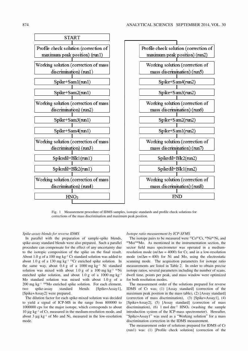
Although the detector of the ICP-SFMS showed a normal value (15 ns) at first, the detector used in the CCQM interlaboratory study presented an unpredictable value in spite of its normal gain (–2000 V). Figure 4 shows the measurement result of the detector dead-time used in the CCQM interlaboratory study. The P versus τ curves were investigated using increasing concentrations (5, 10, 20, 40, 60, 80 ng g–1) of Cr solutions. Chromium was selected as one of the target elements in the present study. The mass spectrometer was operated at the medium-resolution (m/Δm = 4000), free from the spectral interference of 40Ar12C+. The dead-time and its standard uncertainty, calculated from the intersections, were –45 and 5 ns, respectively. For other target elements, Ni and Mo, similar negative dead-times were obtained. During a CCQM interlaboratory study, the dead-time showed a negative value even if the SEM was exchanged for a new one of the same type. In other words, the dead-time showed a negative value regardless of the lifetime of the SEM detector. A negative dead-time means that the number of actually observed ions exceeds that of incident ions. The author thus supposed that some kind of noises besides an incident ion entered the SEM to generate extra counts, resulting in a negative dead-time. As a result of several examinations after the CCQM study, it was found that the reason for the noise current to the SEM was a baseplate (printed board) that applies voltage to the electron multiplier. One of the condensers set at the baseplate had a problem, and then a noise signal was generated continually from there. The dead-time showed a normal value (10 – 30 ns) by replacing the baseplate. The effects of a negative dead-time and its uncertainty on the combined standard uncertainty of analytical results are explained in the following sections.

Mass dependence of the dead-timeAnother important matter to be discussed is the mass

dependence of the detector dead-time. Figure 5 presents the result of dead-time determinations for various elements over a wide mass range. The electron multiplier was different from the detector used in the CCQM interlaboratory study, showing a positive dead-time.

The method of the dead-time determination and the uncertainty estimation was similar to that shown in Fig. 3. For the measurements of Mg, Cu, In, Lu and Pb, the mass spectrometer was operated at low resolution, while for Cr and Fe it was operated at the medium-resolution mode. Considering the

uncertainty of the measurement, the dead-times showed a decrease with increasing mass of the element. The uncertainty of the dead-time for Cr was extremely larger than those of the other elements, probably because of a larger fluctuation effect of the peak top in the mass table in the medium-resolution mode. In such a case of Cr, the use of the dead-time presumed from the other elements would be recommended. These results suggest the necessity of checking the mass dependence of the dead-time when using a new type of detector and/or instrument.

Some reports on this topic have been seen in the literature. Vanhaecke et al.15 compared the behavior of a Channeltron continuous dynode electron multiplier of an ICP-quadrupole mass spectrometer with that of an SEM equipped with an ICP-SFMS by measuring the dead-time for various elements (Mg, Ni, Sr, Ba and Pb). They found a different tendency on the mass dependence of the dead-time; the former detector showed an increasing tendency with increasing mass of the elements, and the latter one showed an almost constant dead-time over the mass range investigated. They interpreted that this difference would be due to not only a difference in the detector type, but also a difference in the mass dependence of the incident ion kinetic energies between quadrupole and sector field mass spectrometers.

On the contrary, Held et al.16 employing an ICP-quadrupole mass spectrometer system with a Channeltron continuous dynode similar to that used by Vanhaecke et al., reported no significant difference of the dead-time due to the masses of the elements, including Mg, Zr, Dy and Pb. In addition, our ICP-SFMS system showed a clear mass dependence of the detector dead-time. Both results of Held and the authors suggest that a similar type of electron multiplier and/or a similar type of ICP-mass spectrometer do not necessarily show the same behavior of mass dependence. However, the mass dependence of the dead-time would be related to the kinetic energies and/or transmission efficiencies of the incident ions, as reported by Vanhaecke et al.

A decreasing tendency of the dead-time with increasing mass of the element, shown Fig. 5, may be the slower velocity of the incident ions for a heavier mass of the element, because electrostatic energies were supposed to be constant for the whole mass range investigated in ICP-SFMS. As a result, the slower velocity would lead to less counting loss is ions.

Fig. 4　Observed 52Cr/53Cr ratio plotted against the applied dead-time obtained for Cr assay solutions with the concentration ranging from 5 to 80 ng g–1.

Fig. 5　Variation of the detector dead-time (◆) as a function of the analyte mass. The analytes are Mg, Cr, Fe, Cu, In, Lu and Pb. Each bar indicates the standard deviation for three determinations.


Effect of a negative dead-time on the result of the CCQM interlaboratory study

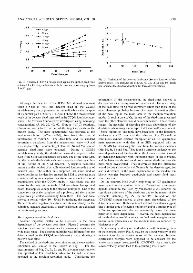
As mentioned above, the dead-time of the detector used in the CCQM interlaboratory study had a negative value of –45 ± 5 ns, in spite of its normal gain. The effects of the negative dead-time and the uncertainty of the detector on the trueness and the precision of the IDMS analytical results were examined through the CCQM interlaboratory study. Table 5 gives the IDMS analytical result of NMIJ and the uncertainty budget of Cr, Ni and Mo in a low-alloy steel, compared with reference values estimated as the simple mean ± standard deviation (1σ) for the results of all participants. No significant difference was observed between our result and the reference value for each element. These comparison results indicate that a precise IDMS analysis can be achieved by correcting the detector dead-time, even if the value of the dead-time would be negative.

Similar precisions of the isotope ratio measurement between low-resolution and medium-resolution can be clearly seen in Table 5. The standard uncertainties, (3) and (7), were related to the repeatabilities of isotope ratio measurements for reverse IDMS and IDMS, respectively. For both cases there were not

significant differences in the uncertainty due to the repeatability of the isotope ratio measurement between Ni (0.041, 0.040) in the low-resolution mode and Cr (0.051, 0.063) in the medium-resolution mode. In the case of Mo, twice or three times-larger uncertainties (0.107, 0.153) than Ni and Cr would be due to a large mass difference (95Mo and 100Mo ) to lead a time loss of mass scanning.

As for Ni, the repeatability for 2 reverse ID blends mainly contributed to the combined uncertainty, probably due to the difference in the concentration between two assay standards. The result of Mo agreed exactly with the average value of the CCQM participants; however, our expanded standard uncertainty went up to 5% due to the uncertainty of the isotopic abundance of Mo. The poorer uncertainty in the measurement of Mo emphasizes that a problem to be solved still remains in IDMS.

The standard uncertainty (9) given in Table 5 was the effect of the uncertainty due to the detector dead-time on the IDMS analytical result. While uncertainties due to the dead-time in the measurement of Ni and Mo were negligibly small (0.025 and 0.015%), that of Cr (0.24%) was the most important factor affecting the combined standard uncertainty of the analytical

Table 5　Analytical results of CCQM interlaboratory study

Analytical results of minor elements of low steel alloy (mass fraction %) Cr Ni Mo

Analytical results of NMIJ, average value ± expanded uncertainty (k = 2) 0.4917 ± 0.0042 1.9793 ± 0.0454 0.9566 ± 0.0493

Average value ± standard deviation of CCQM participants 0.4863 ± 0.0079 1.9690 ± 0.0232 0.9605 ± 0.0143

Standard uncertainty (relative %)

Reverse IDMS

(1) Uncertainty for assay standard u(Cz)/Cz 0.05 0.05 0.05

(2) Uncertainty due to atomic fraction of assay standard

12 2

2′ −

+ − ′

′ −

R d c

u a RR d c

u b( ) ( )

α

0.016 0.018 1.051

(3) Uncertainty due to repeatability of isotope ratio measurementa

bc adR d c

u R−′ −

′( )

( ) )2

2/( α0.051 0.041 0.107

(4) Repeatability of 2 reverse ID blendsa

RSDmean for Cy 0.216 1.142 0.166

(5) Uncertainty of spike concentration [combination of (1), (2), and ((3) or (4))]

u(Cy)/Cy 0.245 1.143 1.805

IDMS (6) Uncertainty due to atomic fraction of sample

− −−

+ −−

( )( )

( ) ( )( )

(Rd ce Rf

u e R Rd ce Rf

u f2

2

2))

2

2β

0.026 0.015 0.911

(7) Uncertainty due to repeatability of isotope ratio measurementb

de cfe Rf

u R−

−( )( ) /( )

22β

0.063 0.040 0.153

(8) Repeatability of 4 ID blendsb RSDmean for Cx 0.237 0.104 0.647

(9) Uncertainty due to detector dead-time ∂γ/γ 0.240 0.025 0.015

Combined standard uncertainty of sample concentration [combination of (5), (6), and ((7) or (8)), and (9)]

u(Cx)/Cx 0.430 1.149 2.575

Expanded Uncertainty (k = 2) 0.861 2.297 5.151

a. Larger one between (3) and (4) was adopted.b. Larger one between (7) and (8) was adopted.


result.The difference between the effect of the uncertainty of the

dead-time for Cr and those for Ni and Mo can be explained by the following theoretical consideration of the IDMS equation as a function of the dead-time τ. When Eq. (6) is substituted in Eq. (5), we obtain

C Cmm

mm

Rd ce Rf

a R bR d c

x zy

x

z

y

= ⋅ ⋅′

⋅ −−

⋅ − ′′ −

. (19)

When the Rd ce Rf

a R bR d c

−−

⋅ − ′′ −

part of Eq. (19) is replaced by γ,

where R and R′ are functions of dead-time τ, γ is expressed as

γ ττ

ττ

= ⋅ −− ⋅

⋅ − ′ ⋅

′ ⋅ −R d ce R f

a b bR d c

( )( )

( )( )

(20)

Here, R(τ ) and R′(τ) are

R I II I

RI I

( ) ( )( )

, ( )(τ τ

ττ τ= − ⋅

− ⋅′ = ′ − ⋅ ′A B

B A

A B11

1 ))( )

.′ − ⋅ ′I IB A1 τ

(21)

IA and IB are the measured signals of IDMS for mass A and mass B; and I′A and I′B are the measured signals of reverse

IDMS for mass A and mass B, respectively.Differentiating Eq. (20) by τ, we obtain

∂∂

=− ⋅ ′ ⋅ −

×

′ ⋅ −

γτ τ τ

τ

12 2( ( ) ) ( ( ) )

( ( ) )(

e R f R d c

R d c a −− ′ ⋅ − ∂∂

+{⋅ − −

R b de cf R

R d c e R

( ) )( ) ( )

( ( ) )( ( )

τ ττ

τ τ ⋅⋅ − ∂ ′∂ }f bc ad R)( ) ( ) .ττ

(22)

Here,

∂ ′∂

= ′′

⋅ ′ − ′− ⋅ ′

∂∂

=R II

I II

R I( )( )

( )ττ τ

ττ

A

B

A B

A

A

1 2 III I

IB

A B

A

⋅ −− ⋅( )

.1 2τ (23)

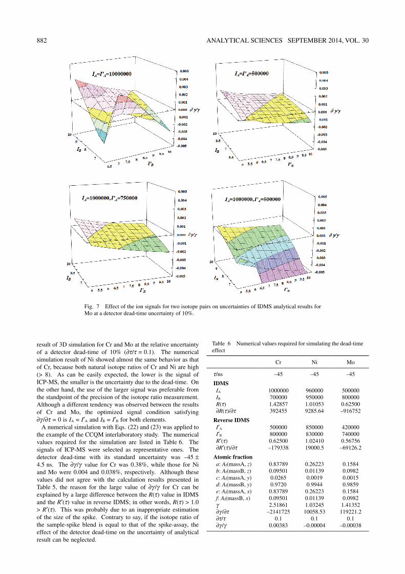
Looking at the middle parenthesis in Eq. (22), it is easily understood that the first and second terms look very much alike. In addition, the value of “de – cf” substantially equals the minus value of “bc – ad” because a ≈ e and b ≈ f. This means that the condition satisfying ∂γ/∂τ = 0 exists. The effect of the uncertainty of the dead-time (∂τ/τ) on the combined standard uncertainty of the analytical result (∂γ/γ) can be computed numerically as functions of the atomic fractions, the signals of ICP-MS and the detector dead-time. Figures 6 and 7 present the

Fig. 6　Effect of the ion signals for two isotope pairs on uncertainties of IDMS analytical results for Cr at the detector dead-time uncertainty of 10%. IA and IB are the measured signals of IDMS for mass A and mass B, and I′A and I′B are measured signals of reverse IDMS for mass A and mass B, respectively.


result of 3D simulation for Cr and Mo at the relative uncertainty of a detector dead-time of 10% (∂τ/τ = 0.1). The numerical simulation result of Ni showed almost the same behavior as that of Cr, because both natural isotope ratios of Cr and Ni are high (> 8). As can be easily expected, the lower is the signal of ICP-MS, the smaller is the uncertainty due to the dead-time. On the other hand, the use of the larger signal was preferable from the standpoint of the precision of the isotope ratio measurement. Although a different tendency was observed between the results of Cr and Mo, the optimized signal condition satisfying ∂γ/∂τ = 0 is IA = I′A and IB = I′B for both elements.

A numerical simulation with Eqs. (22) and (23) was applied to the example of the CCQM interlaboratory study. The numerical values required for the simulation are listed in Table 6. The signals of ICP-MS were selected as representative ones. The detector dead-time with its standard uncertainty was –45 ± 4.5 ns. The ∂γ/γ value for Cr was 0.38%, while those for Ni and Mo were 0.004 and 0.038%, respectively. Although these values did not agree with the calculation results presented in Table 5, the reason for the large value of ∂γ/γ for Cr can be explained by a large difference between the R(τ) value in IDMS and the R′(τ) value in reverse IDMS; in other words, R(τ) > 1.0 > R′(τ). This was probably due to an inappropriate estimation of the size of the spike. Contrary to say, if the isotope ratio of the sample-spike blend is equal to that of the spike-assay, the effect of the detector dead-time on the uncertainty of analytical result can be neglected.

Table 6　Numerical values required for simulating the dead-time effect

Cr Ni Mo

τ/ns –45 –45 –45

IDMSIA 1000000 960000 500000IB 700000 950000 800000R(τ) 1.42857 1.01053 0.62500∂R(τ)/∂τ 392455 9285.64 –916752

Reverse IDMSI′A 500000 850000 420000I′B 800000 830000 740000R′(τ) 0.62500 1.02410 0.56756∂R′(τ)/∂τ –179338 19000.5 –69126.2

Atomic fractiona: Af(massA, z) 0.83789 0.26223 0.1584b: Af(massB, z) 0.09501 0.01139 0.0982c: Af(massA, y) 0.0265 0.0019 0.0015d: Af(massB, y) 0.9720 0.9944 0.9859e: Af(massA, x) 0.83789 0.26223 0.1584f: Af(massB, x) 0.09501 0.01139 0.0982γ 2.51861 1.03245 1.41352∂γ/∂τ –2141725 10058.53 119221.2∂τ/τ 0.1 0.1 0.1∂γ/γ 0.00383 –0.00004 –0.00038

Fig. 7　Effect of the ion signals for two isotope pairs on uncertainties of IDMS analytical results for Mo at a detector dead-time uncertainty of 10%.


Conclusions

The parameters affecting the uncertainty of the analytical results of IDMS are the signal of ICP-MS and the uncertainty of the detector dead-time as well as the uncertainties of the atomic factions in the sample and assay standards, precision of isotope ratio measurements and standard deviations for analytical results of replicates prepared for “double IDMS”. Therefore, the signal intensity of ICP-MS should be carefully selected because the signal intensity of ICP-MS and the detector dead-time have opposite effects on the accuracy of the analytical result. In other words, the larger the signal of ICP-MS, exceeding 106 cps, causes not only better precision of the isotope ratio measurements, but also the poor trueness of the isotope ratio due to the counting loss of ions. In order to reduce the effects of these parameters on the analytical results, both the mixing ratios of the [spike + sample] blend for IDMS and the [spike + assay standard] blend for reverse IDMS and their dilution factors should be carefully determined while considering the atomic fractions of the two isotopes, especially in the case of Mo with similar atomic fractions of the two isotopes. On the other hand the effect of the uncertainty of the detector dead-time can be minimized when the isotope ratio of the [sample + spike] blend for IDMS almost equals that of the [spike + assay standard] blend for reverse IDMS. This conclusion applies even when the dead-time of the detector showed a negative value, as was presented in the analytical result of the CCQM interlaboratory study on low-alloy steel.

The uncertainty budget given in Table 5 will give us useful information about which parameter is the most dominant to the combined uncertainty of the analytical result, and give us a useful guideline on future improvements of the IDMS procedure. Although the uncertainties of the atomic fractions and the detector dead-time are essentially impossible to be lowered, the precision of the isotope ratio measurement and the dispersion for the analytical results of two or four replicates can be improved to a certain extent by artificial efforts. An analytical result with small uncertainty does not necessarily mean a good result. However, possible efforts to reduce the uncertainty would be required so as to make the most of the latent ability of IDMS as the primary method.

Supporting Information

This material is available free of charge on the Web at http://www.jsac.or.jp/analsci/.

References

1. W. Richter, Accred. Qual. Assur., 1997, 2, 354.

2. F. Vanhaecke, L. Moens, R. Dams, I. Papadakis, and P. Taylor, Anal. Chem., 1997, 69, 268.

3. C. Laktoczy, T. Prohaska, G. Stingeder, and M. Teschler-Micola, J. Anal. At. Spectrom., 1998, 13, 561.

4. C. R. Quetel, J. Vogl, T. Prohasca, S. Nelms, P. D. P. Taylor, and P. De Bievre, Fresenius’ J. Anal. Chem., 2000, 368, 145.

5. S. Sturup, H. Dahlgaard, and S. C. Nielsen, J. Anal. At. Spectrom., 1998, 13, 1321.

6. H. Wildner, J. Anal. At. Spectrom., 1998, 13, 573. 7. T. Prohaska, C. Latkoczy, and G. Stingeder, J. Anal. At.

Spectrom., 1999, 14, 1501. 8. A. Makishima and E. Nakamura, J. Anal. At. Spectrom.,

2000, 15, 263. 9. P. Evans and B. Fairman, J. Environ. Monit., 2001, 3, 469. 10. S. Sturup, J. Anal. At. Spectrom., 2002, 17, 1. 11. L. Yang, Z. Mester, L. Abranko, and R. E. Sturgeon, Anal.

Chem., 2004, 76, 3510. 12. J. R. Encinar, J. I. G. Alonso, A. Sanz-Medel, S. Main, and

P. J. Turner, J. Anal. At. Spectrom., 2001, 16, 315. 13. K. E. Murphy, S. E. Long, M. S. Rearick, and O. S. Ertas,

J. Anal. At. Spectrom., 2002, 17, 469. 14. Z. Y. Huang, C. Y. Yang, Z. X. Zhuang, X. R. Wang, and F.

S. C. Lee, Anal. Chim. Acta, 2004, 509, 77. 15. F. Vanhaecke, G. de Wannermacker, L. Moens, R. Dams, C.

Latkoczy, T. Prohasca, and G. Stingerder, J. Anal. At. Spectrom., 1998, 13, 567.

16. A. Held and P. D. P. Taylor, J. Anal. At. Spectrom., 1999, 14, 1075.

17. J. Moser, W. Wegscheider, and T. Meisel, J. Anal. At. Spectrom., 2003, 18, 508.

18. S. J. Hill, L. J. Pitts, and A. S. Fisher, TrAC, Trends Anal. Chem., 2000, 19, 120.

19. The BIPM key comparison database, http://kcdb.bipm.org/AppendixB/KCDB_ApB_search.asp.

20. R. Kaarls and T. J. Quinn, Metrologia, 1997, 34, 1. 21. R. L. Watters, Jr., K. R. Eberhardt, E. S. Beary, and J. D.

Fassett, Metrologia, 1997, 34, 87. 22. N. Nonose, A. Hioki, M. Kurahashi, and M. Kubota,

Bunseki Kagaku, 1998, 47, 239. 23. Isotopic compositions of the elements 2009, Pure Appl.

Chem., 2011, 83, 397. 24. JCGM-100:2008, “Evaluation of measurement data-Guide

to the expression of uncertainty in measurement”. 25. N. Nonose, C. Cheong, Y. Ishizawa, T. Miura, and A. Hioki,

Anal. Chim. Acta, 2014, 840, 10. 26. G. P. Russ, III, in “Applications of Inductively Coupled

Plasma Mass Spectrometry”, ed. A. R. Date and A. L. Gray, 1989, Chap. 4, Blackie, Glasgow and London, 90.

Documents

Effect of the Detector Dead-time Uncertainty on the