Embed Size (px)
Citation preview
This article was downloaded by: [University of Miami]On: 01 October 2013, At: 11:05Publisher: Taylor & FrancisInforma Ltd Registered in England and Wales Registered Number: 1072954 Registered office: MortimerHouse, 37-41 Mortimer Street, London W1T 3JH, UK
Journal of Hydraulic ResearchPublication details, including instructions for authors and subscription information:http://www.tandfonline.com/loi/tjhr20
Effect of selected parameters on the depositionalbehaviour of turbidity currentsEhsan Khavasi a , Hossein Afshin b & Bahar Firoozabadi ca Department of Mechanical Engineering, Sharif University of Technology, Tehran, Iran E-mail:b Department of Mechanical Engineering, Sharif University of Technology, Tehran, Iran E-mail:c Department of Mechanical Engineering, Sharif University of Technology, Tehran, IranPublished online: 07 Dec 2011.
To cite this article: Ehsan Khavasi , Hossein Afshin & Bahar Firoozabadi (2012) Effect of selected parameterson the depositional behaviour of turbidity currents, Journal of Hydraulic Research, 50:1, 60-69, DOI:10.1080/00221686.2011.641763
To link to this article: http://dx.doi.org/10.1080/00221686.2011.641763
PLEASE SCROLL DOWN FOR ARTICLE
Taylor & Francis makes every effort to ensure the accuracy of all the information (the “Content”) containedin the publications on our platform. However, Taylor & Francis, our agents, and our licensors make norepresentations or warranties whatsoever as to the accuracy, completeness, or suitability for any purpose ofthe Content. Any opinions and views expressed in this publication are the opinions and views of the authors,and are not the views of or endorsed by Taylor & Francis. The accuracy of the Content should not be reliedupon and should be independently verified with primary sources of information. Taylor and Francis shallnot be liable for any losses, actions, claims, proceedings, demands, costs, expenses, damages, and otherliabilities whatsoever or howsoever caused arising directly or indirectly in connection with, in relation to orarising out of the use of the Content.
This article may be used for research, teaching, and private study purposes. Any substantial or systematicreproduction, redistribution, reselling, loan, sub-licensing, systematic supply, or distribution in anyform to anyone is expressly forbidden. Terms & Conditions of access and use can be found at http://www.tandfonline.com/page/terms-and-conditions

Journal of Hydraulic Research Vol. 50, No. 1 (2012), pp. 60–69http://dx.doi.org/10.1080/00221686.2011.641763© 2012 International Association for Hydro-Environment Engineering and Research
Research paper
Effect of selected parameters on the depositional behaviour of turbidity currentsEHSAN KHAVASI, PhD Student, Department of Mechanical Engineering, Sharif University of Technology, Tehran, Iran.Email: [email protected]
HOSSEIN AFSHIN, Assistant Professor, Department of Mechanical Engineering, Sharif University of Technology, Tehran, Iran.Email: [email protected]
BAHAR FIROOZABADI, Professor, Department of Mechanical Engineering, Sharif University of Technology, Tehran, Iran.Email: [email protected] (author for correspondence)
ABSTRACTTurbidity currents containing kaolin particles were studied experimentally in a channel and the velocity and concentration profiles were measured usingan acoustic Doppler velocimeter. These experiments were performed to investigate the depositional behaviour of turbidity currents. The suspendedsediment flux was evaluated by experimental and analytical methods and the results of these two methods were in a good agreement. To evaluate thesuspended sediment flux, it was necessary to recognize the suspended sediment zone from the upper shear layer region and near the bed depositionalarea as well. The method of determination of these areas is discussed. The effects of important parameters including the inlet Froude number and bedslope were also studied. Based on these results, it can be concluded that the non-dimensional sediment flux decreases at the vicinity of the hydraulicjump with the inlet Froude number, whereas an increase in the bed slope reduces the non-dimensional sediment flux.
Keywords: Deposition, inlet Froude number, suspended sediment flux, turbidity current
1 Introduction
Turbidity currents develop because of the gravitational force act-ing on the density difference due to suspended particles in theflow. Because of the gravitational force acting on this type of cur-rents, they are a subcategory of gravity currents. Fluid turbulenceof the flow holds the sediments in suspension (Middleton 1993),although it is believed that this is not a true statement; in turn,the flow turbulence appears to be re-suspending the sedimentsdeposited on the bed (Toniolo et al. 2006); this effect makes thesecurrents erosive as well. Oceans, lakes and reservoirs are placeswhere turbidity currents occur (Garcia 1994). They are relevantin relation to sediment transport into subaqueous environments(Meiburg and Kneller 2009). Erosion of underwater canyons alsotakes place due to turbidity currents. The damage of submarinecables and the formation of tsunamis are due to these currents(Simpson 1982). Layers of deposits created by compacted anddeeply buried turbidity currents can serve as good hydrocarbonreservoirs (Meiburg and Kneller 2009, Toniolo et al. 2006). Fur-thermore, turbidity currents are the agents of a large amount ofreservoir sedimentation (De Cesare et al. 2001).
The importance of turbidity currents has encouraged manyresearchers to study these currents. Bell (1942) demonstrated thatthese currents have an important role in reservoir sedimentation.Ellison and Turner (1959) studied the body of the currents, find-ing that the entrainment from the ambient fluid into the denselayer is a function of the overall Richardson number. Middle-ton (1993) reviewed the role of sediment deposition, includingthe capability of turbidity currents for deposition and erosion.He concluded that their properties can be measured both in thelaboratory and in nature by interpreting the deposits.
The non-dimensional parameters of turbidity currents includethe Reynolds number, R, and the densimetric Froude or the bulkRichardson number as the reciprocal of the square of the densi-metric Froude number F = U/(g′h cos θ)0.5. Here, the reducedgravity acceleration is g′ = g(ρ − ρw)/ρw, in which ρ is themixture density, ρw is the ambient water density and g is thegravitational acceleration, U is average velocity, h is the averagecurrent height and R = ρUh/μ with μ as dynamic viscosity ofthe dense fluid. Because of the small density difference betweenwater and the dense fluid, the dynamic viscosity of the current isapproximately equal to that of water, based on Roscoe’s (1952)
Revision received 14 November 2011/Open for discussion until 31 August 2012.
ISSN 0022-1686 print/ISSN 1814-2079 onlinehttp://www.tandfonline.com
60
Dow
nloa
ded
by [
Uni
vers
ity o
f M
iam
i] a
t 11:
05 0
1 O
ctob
er 2
013

Journal of Hydraulic Research Vol. 50, No. 1 (2012) Depositional behaviour of turbidity currents 61
Figure 1 Definition sketch of an internal hydraulic jump
expression. Non-dimensional numbers determine the regime ofturbidity currents.
These currents experience a hydraulic jump from supercrit-ical to subcritical flow (Middleton 1993) along with suddenenergy dissipation. As the current height increases, the fluidslows down creating an area of turbulence. The non-dimensionalquantity characterizing the hydraulic jump is the Froude number.Three flow regimes may occur: subcritical (Fin < Fc), critical(Fin = Fc) and supercritical (Fin > Fc). In open-channel flows,the critical (subscript c) Froude number is Fc = 1. However, itsvalue may be different in internal hydraulic jumps and is deter-mined from experiments (Huang et al. 2009). Figure 1 shows aschematic sketch of an internal hydraulic jump.
Garcia (1993) conducted experiments in a flume of vari-able slope and studied the behaviour of turbidity currents nearthe slope transition. He noted that the vertical current structuredepends on the flow regime.
Kneller and Buckee (2000) reviewed the gravity currentsbased on turbidity currents. They found that the velocity profilesin natural and experimental gravity currents are similar to thoseof plane turbulent wall jets. The corresponding concentrationprofiles were also studied.
The deposition and erosion are important features of turbid-ity currents affecting the environment. Garcia (1993) observedthat the flow regime changes from supercritical to subcriticalflow through an internal hydraulic jump. In his setup, the bedslope was 8% for the supercritical portion and horizontal for thesubcritical portion. For coarse sediment, the deposition decaysexponentially.
Kostic and Parker (2006) found that the response of turbid-ity currents to a canyon–fan transition caused internal hydraulicjumps and changed the depositional signatures numerically. Theyfound that the internal hydraulic jump leads to a step-like increasein sediment deposits. Furthermore, their study showed that anincrease in the canyon slope decreases sediment deposit.
Fang and Rodi (2003) proposed a three-dimensional computercode to calculate the flow and suspended sediment transport neara dam. For both velocity and the bed level developments, therewas a good agreement between the experimental data and thenumerical results.
In the previous works, the structure of the deposition, theeffect of sediment size and the topography on the deposition andthe impact of the deposition on the behaviour of the currentswere accounted for. However, the effects of the inlet Froudenumber and the bed slope on the depositional behaviour wereoverlooked and so they are considered below. An analyticalapproach is introduced to calculate the non-dimensional sedi-ment flux. The concept was adopted from previous works onopen-channel flows. The dimensionless sediment flux was deter-mined using universal velocity and concentration profiles of theexamined currents. The approach is validated by experimentaldata to discuss the depositional behaviour.
2 Experimental setup
2.1 Test setup
A laboratory apparatus was used to study the two-dimensionalflows resulting from the release of sediment-laden densitycurrents on a sloping surface in a fresh water channel. The chan-nel was 12 m long, 0.20 m wide and 0.60 m deep. One side of thechannel was made of glass for visual observation. The channelwas divided into two sections in the longitudinal direction usinga separating Plexiglas sheet referred to as the gate in Fig. 2.A particle-laden fluid was accumulated in the shorter upstreamportion with a sluice gate. A supply pipe fed the particle-ladenfluid from a reservoir into the accumulator. A gate valve com-bined with a discharge meter controlled the constant feed rate.After kaolin had mixed with water in the reservoir and beforefeeding it into the accumulator, the mixture was transferred to aweir to keep the particle-laden fluid head constant and to preventfluctuations in the feed rate.
The adjustable gate allowed to vary the inlet velocity of theparticle-laden fluid. Its openings were 40, 50, 60 and 70 mm.The channel was filled previously with fresh water at laboratorytemperature. By removing the gate at the start of the test, theparticle-laden fluid was continuously fed into the accumulatorthrough the gate and then it was allowed to flow down the sloping
Figure 2 Schematic side view of test setup
Dow
nloa
ded
by [
Uni
vers
ity o
f M
iam
i] a
t 11:
05 0
1 O
ctob
er 2
013

62 E. Khavasi et al. Journal of Hydraulic Research Vol. 50, No. 1 (2012)
bottom at either 1% or 2%. The density current gradually spreadunder the fresh water. At the end of the channel, the particle-laden fluid impacted a back step and was withdrawn through thebottom drains.
To avoid a return flow, a 25-cm-high step was located at theoutlet. Sixty-four valves, each with a discharge of 0.6 l/min,were located under the step surface. The number of open valvesdepended on the inlet discharge. The outflow was set equal tothe inflow and kept constant during the test.
Kaolin of density ρ = 2650 kg/m3 and D50 ∼ 12 μ was usedas a suspension. Its density was measured with a hydrometer priorto supply, but the mixed flow density was not measured. Veloc-ity profiles were recorded by a remote-sensing 10 MHz acousticDoppler velocimeter (ADV) of Nortek�. This device measuresall three velocity components to ±0.1 mm/s. It was positioned in120◦ increments on a circle around the transmitter and slanted at30◦ from the axis of the transmit transducer. The echo reflectedfrom the particles suspended in the flow was assumed to movewith water velocity. The strength of the echo was quantified interms of a signal-to-noise ratio (SNR) expressed in dB. The man-ufacturer recommends SNR>15 dB for a 25 Hz sampling rate ofthe raw data.
The scattered sound signal detected by the receivers deter-mined the Doppler shift. The flow velocity follows from thisshift in the ultrasound frequency, as particles pass through themeasurement volume. The shape of the sample volume is cir-cular cylindrical with 6 mm diameter and about 9 mm height, sothat its volume is about 0.25 cm3. It is located 50–100 mm fromthe transmitter tip.
The concentration profiles were obtained by ADV probesusing the ABS theory (Nikora and Goring 2002). This theoryis based on the amplitude of waves scattering from the particlesin the flow. The ADV probes gave the amplitude of the scatter-ing waves in the NDV software developed by Nortek to performADV data acquisition. The equation c(z) = P × 100.0434A con-verts the amplitudes A to the concentration, where Pis thecalibration parameter and c(z) is the local concentration. Themeasurements were taken starting at the top of the current andwere continued towards the lower part by lowering the probes.About 14 positions were used to obtain the velocity profile ateach station. This work involved two station pairs. By using thetwo probes, the velocities were measured simultaneously at twostations spaced by 1 m. The total test duration was about 1 h.Preliminary tests were conducted to study the variation in thevelocity profiles, and yet no significant effect was observed.
The velocity profiles were measured at six stations in theflow direction, located at x = 0.5, 1.5, 2.5, 3.5, 4.5 and 5.5 m,where x is the distance of the ADV from the inlet. The resultsobtained at x = 0.5 m were excluded because of the strong inletdisturbances. The coordinate x was non-dimensionalized by thechannel length L.
The inlet discharge was always Q = 35.6 l/min, resulting inthe inlet Reynolds number of Rin = Q/bυ = 2930, with b and υ
as the channel width and kinematic viscosity of the inlet mixture,
Table 1 Inlet conditions for all experiments
S U0 h0 C0Run (%) (cm/s) (cm) (g/l) Fin
1 1 7.39 4 1 3.62 1 7.39 4 1.5 33 1 7.39 4 4 1.84 1 5.93 5 0.88 3.65 1 5.93 5 1.28 36 1 5.93 5 2.88 27 1 5.93 5 4.8 1.58 1 5.93 5 6.83 1.39 1 5.93 5 9.55 1.1
10 1 4.942 6 0.51 3.611 1 4.942 6 0.74 312 1 4.942 6 1.66 213 1 4.942 6 2.76 1.514 1 4.942 6 3.95 1.315 1 4.942 6 6.68 116 1 4.23 7 1 217 1 4.23 7 1.75 1.518 1 4.23 7 2.5 1.319 1 4.23 7 4.2 123 2 7.39 4 1.75 3.624 2 7.39 4 2.5 325 2 7.39 4 6.5 1.826 2 4.23 7 1 227 2 4.23 7 1.75 1.528 2 4.23 7 2.5 1.329 2 4.23 7 4.2 1
respectively. The inlet conditions for all experiments are listedin Table 1, with h0 as the inlet opening height, U0 as the averageinlet velocity, C0 as the weight percentage inlet concentration, Sas the bottom slope and Fin as the inlet Froude number.
3 Results and discussions
3.1 Velocity and concentration profiles
Velocity profiles
The purpose of this part is to introduce the universal velocityand concentration profiles of the current to determine the sus-pended sediment flux, which is explained in the next subsection.To investigate complex flows, proving that a flow has a similaritybehaviour helps to deal with the flow structure. In Fig. 3, non-dimensional velocity profiles are shown. Their trend follows thenon-dimensionalized profile.
The general shape of the velocity profile of turbidity currentsis similar to that of the velocity profile of turbulent plane walljets (Kneller and Buckee 2000). These have an inner and anouter region. The maximum velocity separates the two regions.The inner region is with respect to the rigid boundary on thebottom, whereas the outer region is with respect to the interfaceor diffusion boundary on top of the maximum velocity. In theinner region, the flow is mainly controlled by bottom friction.The velocity distribution follows a logarithmic or an empirical
Dow
nloa
ded
by [
Uni
vers
ity o
f M
iam
i] a
t 11:
05 0
1 O
ctob
er 2
013

Journal of Hydraulic Research Vol. 50, No. 1 (2012) Depositional behaviour of turbidity currents 63
power relation as (Altinakar et al. 1996)
u(z)Um
=(
zHm
)1/αv
(1)
where Um is the maximum velocity, Hm is its height, u(z) is themean streamwise velocity at distance z above the bed and αv isan exponent.
The effect of friction at the top boundary on the velocity pro-file is included by modelling a dense stratified layer of limitedthickness between two homogenous fluids (Kneller et al. 1999).As mentioned by Altinakar et al. (1996), the velocity profile inthe outer region is determined by the semi-Gaussian equation
u(z)Um
= exp[−βv
(z − Hm
H − Hm
)γv]
(2)
where βv and γv are empirical constants and H is the layer-averaged height (to be defined below). Equations (1) and (2)were fitted to the measured velocity profiles at the inner andouter current regions to determine the constants αv , βv and γv .
The constant αv varies considerably, namely from 3.9 to 7.The large scatter appears to be due to particle concentration. Withincreasing concentration, the viscosity increases and thereby theReynolds number decreases so that αv also decreases. The con-stant βv varies between 0.43 and 0.88. The average to be usedin Eq. (2) is 0.6, despite 1.4 being suggested by Altinakar et al.(1996). The constant γv varies between 1.75 and 3.89. The aver-ages of these constants are listed in Table 2 and compared withthose reported by Altinakar et al. (1996). Note that their exper-iments were performed using the inlet Froude numbers rangingfrom 1 to 2.33. Herein, however, the range of Fin varied between1 and 3.6. Even though the data are scattered, the agreementbetween the data of the two studies is reasonably good in viewof the experimental difficulties involved.
Using the average values given in Table 2, the inner and outervelocity profiles were derived. Figure 3 shows that (Nourmo-hammadi et al. 2011)
u(z)Um
=(
zHm
)1/5.8
(3)
u(z)Um
= exp
[−0.6
(z − Hm
H − Hm
)2.7]
(4)
Table 2 Comparison of the present experimental values withthose reported by Altinakar et al. (1996)
Constant αv βv γv
Present 5.8 0.6 2.7Altinakar et al. (1996) 6 1.4 2
Figure 3 Non-dimensional velocity profile u(z)/Um versus(z − Hm)/(H − Hm) or z/Hm
Figure 4 Non-dimensional concentration profile c(z)/Cm versus(z − Hm)/(H − Hm) or z/Hm
Concentration profiles
A stratification of the current was observed in all concentrationprofiles, involving a lower layer of high concentration gradientlocated between the rigid boundary and the height of maximumvelocity (0 < z < Hm) and a homogenous layer of less concen-tration mixing with the ambient fluid in the upper portion of thecurrent.
The concentration profiles were non-dimensionalized withheight Hm and the corresponding concentration Cm. Similar tothe velocity profile, a non-dimensional similarity profile for themean concentration distribution was proposed (Fig. 4) for theouter layer as the semi-Gaussian profile:
c(z)cm
= exp[−βc
(z − Hm
H − Hm
)γc]
(5)
For the concentration distribution in the inner region, thepresent data suggest a power law with αc as the empiricalexponent:
c(z)Cm
=(
zHm
)−ac
(6)
Dow
nloa
ded
by [
Uni
vers
ity o
f M
iam
i] a
t 11:
05 0
1 O
ctob
er 2
013

64 E. Khavasi et al. Journal of Hydraulic Research Vol. 50, No. 1 (2012)
Table 3 Comparison of the present experimental values withthose reported by Altinakar et al. (1996) for concentration profiles
Constant αc βc γc
Present 0.2 2 1.4Altinakar et al. (1996) – 2.4 1.3
This relation is valid for the region between the depositional areaand the height of maximum velocity. In the depositional area, theconcentration profile is meaningless.
To complete the above relations for the proposed concentra-tion profile in turbidity currents, the constants αc, βc and γc haveto be determined. Constant αc varies between 0.15 and 0.28, withthe average of 0.2. The constant βc scatters in the range of 1–3.1,with 2 being suggested as the average value. The correspondingrange reported by Altinakar et al. (1996) was between 1.7 and4.1. γc varies between 1.1 and 1.7 with the average of 1.4, whichis close to 1.3, as proposed by Altinakar et al. (1996). The aver-ages of these constants are given in Table 3. If introduced in therelations for the concentration distributions, the two general rela-tions for the concentration profiles of the inner and outer regionsare (Nourmohammadi 2008)
c(z)Cm
=(
zHm
)−0.2
(7)
c(z)Cm
= exp
[−2.0
(z − Hm
H − Hm
)1.4]
(8)
3.2 Vertical structure of turbidity currents
The main purpose of this research was to study the effects ofthe inlet Froude number and the bed slope on the depositionalbehaviour of turbidity currents. An analytical method developedfrom the concepts of open-channel flows was applied to obtainthe suspended sediment flux. The suspended sediment flux wascalculated so that the non-dimensional sediment flux and thedepositional behaviour of turbidity currents resulted. First, theregion of suspended sediment was distinguished from others bydividing the current into finite parts. The two regions based onthe maximum current velocity include (similar to turbulent walljets) the inner region located below and the outer region abovethe maximum velocity (Kneller and Buckee 2000, Meiburg andKneller 2009).
A density current (or saline underflow) may also be dividedinto four layers: (1) boundary layer in which bottom frictionproduces turbulence, (2) bottom layer below the density inter-face, (3) density interface in which a sharp density gradient isobserved and (4) a shear layer (Dallimore et al. 2001). Herein, anew division was defined to show the suspended sediment zoneexplicitly. Based on the concentration profile of a turbidity cur-rent, the dense layer in the normal direction was divided intothree regions: (1) upper shear layer region in which the density
(3)
z/H
u/U or c/C
(1)
(4)
Umax0
(2)
Figure 5 Non-dimensional velocity (–) and concentration (—) profilesdefining three zones: (1) upper shear layer, (2) suspended sediment zoneand (3) depositional area. Observed current height (4) is the height inwhich the density difference or concentration tends to zero
difference reduces to zero, resulting in the entrainment of freshwater into the current (Dallimore et al. 2001); note that this layeris different from the bottom shear layer; (2) suspended sedimentzone, in which the sediments are suspended and flow turbulenceis the main agent for sediment suspension (Kneller and Buckee2000) and (3) depositional area, where particles are likely to settleand deposit on the bottom. These three zones are schematicallyshown in Fig. 5. The current height, velocity and concentra-tion are non-dimensionalized by the average layer height H , theaverage velocity U and the average concentration C, respec-tively, which are defined below. Note that the observed currentheight is the location at which the concentration reduces to zero,corresponding to the thickness of the dense layer.
Upper shear layer
There is a sharp density difference between the main current bodyand pure water in turbidity currents. Above it, both velocity anddensity tend to zero. This layer is known as the upper shearlayer (Dallimore et al. 2001). Sediments diffuse into this layer,which may be erroneously included in the suspended sedimentflux. Therefore, it is necessary to set a criterion to distinguish theupper shear layer from the main current body.
Felix (2004) and Firoozabadi et al. (2009) considered threecharacteristic thicknesses, namely (Fig. 6) (i) z1/2 as the heightabove the velocity maximum Umax, where U = Umax/2, (ii) z1/4
as the height above Umax, where U = Umax/4, and (iii) H asthe layer-averaged height, where H is defined as (Ellison andTurner 1959)
H = (∫ ∞
0 u(z)dz)2∫ ∞0 u(z)2dz
(9)
These characteristic thicknesses are shown in Fig. 6 alongwith the observed current height in which the density differencereduces to zero (Fig. 5). To select the optimum observed heightamong these three alternatives, they were compared with theobservations of Firoozabadi et al. (2009), from which z1/4 wasretained.
Dow
nloa
ded
by [
Uni
vers
ity o
f M
iam
i] a
t 11:
05 0
1 O
ctob
er 2
013

Journal of Hydraulic Research Vol. 50, No. 1 (2012) Depositional behaviour of turbidity currents 65
Depositional area
To determine the suspended load zone, its upper boundary wasanalysed previously . The upper boundary is determined by z1/4.
Umax0.5Umax0 0.25Umax
u or c
z
(1)
z1/4Hz1/2
Figure 6 Velocity (–) and concentration (—) profiles along with threecharacteristic thicknesses and observed height and observed currentheight (1) (density current thickness)
To exclude the deposited sediments or bed load from the calcula-tion among the suspended sediment fluxes, they are distinguishedfrom suspended sediments. The zone of deposited sedimentsis called the “depositional area”. As the particles settle down,they accumulate, resulting in a sudden increase in density (con-centration) as observed in the concentration distribution profile.The depositional area and suspended sediment zone are thusdetermined by the concentration profile.
The non-dimensional concentration and velocity profilesare non-dimensionalized by their averages defined as (Garcia1993)
U =∫ ∞
0 u(z)2dz∫ ∞0 u(z)dz
(10)
C =∫ ∞
0 c(z)u(z)dz∫ ∞0 u(z)dz
(11)
(a) (b)
(c) (d)
(e) (f)
0
1
2
3
4
-0.5 0 0.5 1 1.5
z/H
u/U
z/H = 0.1 , u/U =1.08
0
1
2
3
4
0 1 2 3
z/H
c/C
z/H = 0.1 , c/C = 1.95
0
1
2
3
4
-0.5 0 0.5 1 1.5
z/H
u/U
z/H = 0.3, u/U = 1.25
0
1
2
3
4
0 1 2 3z/
H
c/C
z/H =0.3 , c/C =1.81
0
1
2
3
4
-0.5 0 0.5 1 1.5
z/H
u/U
z/H = 0.25, u/U = 1.2
0
1
2
3
4
0 1 2 3
z/H
c/C
z/H = 0.25, c/C = 1.76
0
1
2
3
4
-0.5 0 0.5 1 1.5
z/H
u/U
z/H = 0.3, u/U = 1.08
0
1
2
3
4
0 1 2 3
z/H
c/C
z/H = 0.3, c/C = 1.6
0
1
2
3
4
-0.5 0 0.5 1 1.5
z/H
u/U
z/H = 0.11, u/U = 1.06
0
1
2
3
4
0 1 2 3
z/H
c/C
z/H = 0.11, c/C = 2.3
0
1
2
3
4
-0.5 0 0.5 1 1.5
z/H
u/U
z/H = 0.2, u/U = 1.1
0
1
2
3
4
0 1 2 3
z /H
c/C
z/H = 0.2, c/C = 1.73
Figure 7 Near-bed depositional area based on velocity (left) and concentration (right) profiles: (a) Run 3, (b) Run 7, (c) Run 8, (d) Run 9, (e) Run13 and (f) Run 14
Dow
nloa
ded
by [
Uni
vers
ity o
f M
iam
i] a
t 11:
05 0
1 O
ctob
er 2
013

66 E. Khavasi et al. Journal of Hydraulic Research Vol. 50, No. 1 (2012)
The corresponding height, concentration and velocity of thedepositional area boundary to their averages z/H , c/C andu/Uare shown in Fig. 7. Their averages and standard deviationsindicate that the lower boundary of the suspended sediment zoneis where u/U = 1.07 ± 0.008 or z/H = 0.20 ± 0.002.
3.3 Depositional behaviour of turbidity currents
The upper shear layer and the near-bed depositional areaswere introduced previously. The suspended sediment zone is,therefore, located between these two so that the suspended sed-iment zone is now recognized. To investigate the depositionalbehaviour of turbidity currents, the suspended sediment fluxwas evaluated. Assuming that all sediments are in suspensionat the inlet, a change in the suspended sediment flux in eachstation when compared with its initial value corresponds to adepositional change along space. The suspended sediment flux
is defined as
qs =∫ ∞
lbc(z)u(z)dz (12)
where lb is the lower boundary of the suspended sediment zoneas defined previously. By comparing qs with its inlet value, thenon-dimensional sediment flux is determined.
To obtain the suspended sediment flux, two approaches wereadopted. In the first experimental method, the concentrations andvelocities obtained by the ADV were introduced into Eq. (12) toevaluate qs. In the second analytical method, qs was obtainedby using velocity and concentration profiles given in the pre-vious subsections and by evaluating the integral numerically.The comparison between these two is shown in Fig. 8, indicat-ing a good agreement in most cases (±10%). Note that qs isnon-dimensionalized by its inlet value qsin .
By calculating the difference between the suspended sedimentfluxes at each station and the inlet value, the new parameter
(a) (b) (c) (d)
(e) (f) (g) (h)
(i) (j) (k) (l)
0
1
2
0 0.25 0.5
q s/q
s(in
)
x/L
0
1
2
0 0.25 0.5
q s/q
s (in
)
x/L
0
1
2
0 0.25 0.5
q s/ q
s(in
)
x/L
0
1
2
0 0.25 0.5q s
/ qs(
in)
x/L
0
1
2
0 0.25 0.5
q s/q
s(in
)
x/L
0
1
2
0 0.25 0.5
q s/q
s(in
)
x/L
0
1
2
0 0.25 0.5
q s/q
s(in
)
x/L
0
1
2
0 0.25 0.5
q s/ q
s(in
)
x/L
0
1
2
0 0.25 0.5
q s/q
s(in
)
x/L
0
1
2
0 0.25 0.5
q s/q
s(in
)
x/L
0
1
2
0 0.25 0.5
q s/q
s(in
)
x/L
0
1
2
0 0.25 0.5
q s/q
s(in
)
x/L
Figure 8 Comparison between experimental (•) and analytical (�) results for qs. (a)–(i) equal to Runs 1–12, respectively
Dow
nloa
ded
by [
Uni
vers
ity o
f M
iam
i] a
t 11:
05 0
1 O
ctob
er 2
013

Journal of Hydraulic Research Vol. 50, No. 1 (2012) Depositional behaviour of turbidity currents 67
(c)(b)(a)
(f)(e)(d)
(i)(h)(g)
0
1
0 0.25 0.5
Ws
x/L
0
1
0 0.25 0.5
Ws
x/L
0
1
0 0.25 0.5
Ws
x/L
0
1
0 0.25 0.5
Ws
x/L
0
1
0 0.25 0.5
Ws
x/L
0
1
0 0.25 0.5
Ws
x/L
0
1
0 0.25 0.5
Ws
x/L
0
1
0 0.25 0.5
Ws
x/L
-1
0
1
0 0.25 0.5
Ws
x/L
Figure 9 Non-dimensional sediment flux illustrating general depositional behaviour: (a) Run 7, (b) Run 9, (c) Run 11, (d) Run 16, (e) Run 17, (f)Run 18, (g) Run 26, (h) Run 28 and (i) Run 29
non-dimensional sediment flux is
Ws = qsin − qs
qsin
(13)
The non-dimensional fluxes along the channel for selected runsare shown in Fig. 9. At x/L = 0.125 with a hydraulic jump closeto this station due to the inlet jet, the current’s ability to carryand suspend the sediment was remarkable as also the erosionand sediment lift-up at its neighbourhood. Thus, the suspendedsediment flux there was high and consequently Ws < 0 (Fig. 9g).
Beyond the jump, the ability to suspend and carry thesediments reduced because of a sudden reduction in the bed-shear stress (Garcia 1993) and a decrease in inertia, so thatthe sediments settled; the suspended sediment flux reduced,
therefore, beyond the jump and the non-dimensional sedimentflux increased. Due to the bed slope, the streamwise velocityincreased gradually and the ability of the current to suspendand carry the sediments increased too. Therefore, the non-dimensional sediment flux reduced. This depositional behaviouragrees qualitatively with the results reported by Alexander andMulder (2002).
Effect of the inlet Froude number on deposition
The non-dimensional sediment flux for So = 2% and various Fin
is shown in Fig. 10, indicating that the non-dimensional sedimentflux reduces near the jump as Fin increases (i.e. at x/L = 0.125).Just beyond the jump (x/L = 0.2), as the hydraulic energy lossdue to the hydraulic jump increases with Fin, the non-dimensional
Dow
nloa
ded
by [
Uni
vers
ity o
f M
iam
i] a
t 11:
05 0
1 O
ctob
er 2
013
68 E. Khavasi et al. Journal of Hydraulic Research Vol. 50, No. 1 (2012)
-1
0
1
0 0.25 0.5
Ws
x / L
Figure 10 Depositional behaviour of current Ws(x/L) for Fin = 2(–�–), 1.3 (–�–) and 1(.•.)
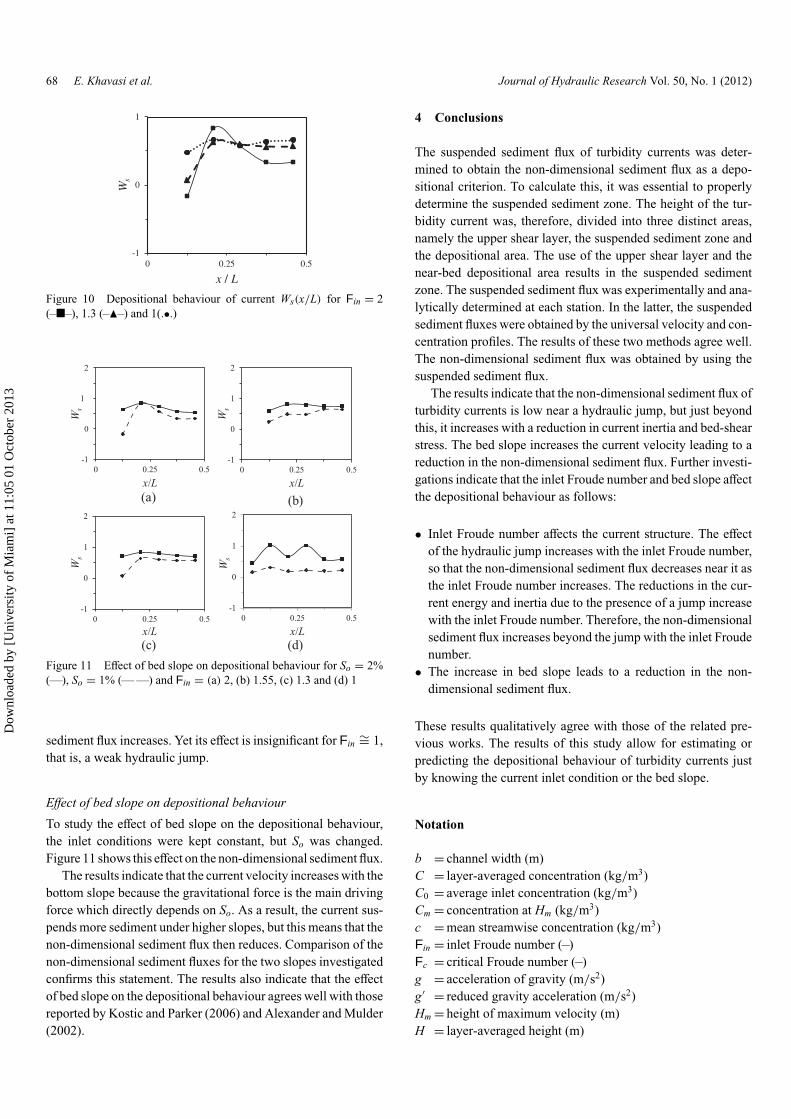
Figure 11 Effect of bed slope on depositional behaviour for So = 2%(—), So = 1% (— —) and Fin = (a) 2, (b) 1.55, (c) 1.3 and (d) 1
sediment flux increases. Yet its effect is insignificant for Fin ∼= 1,that is, a weak hydraulic jump.
Effect of bed slope on depositional behaviour
To study the effect of bed slope on the depositional behaviour,the inlet conditions were kept constant, but So was changed.Figure 11 shows this effect on the non-dimensional sediment flux.
The results indicate that the current velocity increases with thebottom slope because the gravitational force is the main drivingforce which directly depends on So. As a result, the current sus-pends more sediment under higher slopes, but this means that thenon-dimensional sediment flux then reduces. Comparison of thenon-dimensional sediment fluxes for the two slopes investigatedconfirms this statement. The results also indicate that the effectof bed slope on the depositional behaviour agrees well with thosereported by Kostic and Parker (2006) and Alexander and Mulder(2002).
4 Conclusions
The suspended sediment flux of turbidity currents was deter-mined to obtain the non-dimensional sediment flux as a depo-sitional criterion. To calculate this, it was essential to properlydetermine the suspended sediment zone. The height of the tur-bidity current was, therefore, divided into three distinct areas,namely the upper shear layer, the suspended sediment zone andthe depositional area. The use of the upper shear layer and thenear-bed depositional area results in the suspended sedimentzone. The suspended sediment flux was experimentally and ana-lytically determined at each station. In the latter, the suspendedsediment fluxes were obtained by the universal velocity and con-centration profiles. The results of these two methods agree well.The non-dimensional sediment flux was obtained by using thesuspended sediment flux.
The results indicate that the non-dimensional sediment flux ofturbidity currents is low near a hydraulic jump, but just beyondthis, it increases with a reduction in current inertia and bed-shearstress. The bed slope increases the current velocity leading to areduction in the non-dimensional sediment flux. Further investi-gations indicate that the inlet Froude number and bed slope affectthe depositional behaviour as follows:
• Inlet Froude number affects the current structure. The effectof the hydraulic jump increases with the inlet Froude number,so that the non-dimensional sediment flux decreases near it asthe inlet Froude number increases. The reductions in the cur-rent energy and inertia due to the presence of a jump increasewith the inlet Froude number. Therefore, the non-dimensionalsediment flux increases beyond the jump with the inlet Froudenumber.
• The increase in bed slope leads to a reduction in the non-dimensional sediment flux.
These results qualitatively agree with those of the related pre-vious works. The results of this study allow for estimating orpredicting the depositional behaviour of turbidity currents justby knowing the current inlet condition or the bed slope.
Notation
b = channel width (m)C = layer-averaged concentration (kg/m3)C0 = average inlet concentration (kg/m3)Cm = concentration at Hm (kg/m3)c = mean streamwise concentration (kg/m3)Fin = inlet Froude number (–)Fc = critical Froude number (–)g = acceleration of gravity (m/s2)g′ = reduced gravity acceleration (m/s2)Hm = height of maximum velocity (m)H = layer-averaged height (m)
Dow
nloa
ded
by [
Uni
vers
ity o
f M
iam
i] a
t 11:
05 0
1 O
ctob
er 2
013

Journal of Hydraulic Research Vol. 50, No. 1 (2012) Depositional behaviour of turbidity currents 69
h0 = inlet opening height (m)qs = suspended sediment flux (kg/ms)qsin = inlet suspended sediment flux (kg/ms)Rin = inlet Reynolds number (–)So = bed slope (–)U = layer-averaged velocity (m/s)U0 = average inlet velocity (m/s)Um = maximum velocity (m/s)u = mean streamwise velocity (m/s)Ws = non-dimensional sediment flux (–)x = streamwise distance (m)z = vertical coordinate (m)μ = dynamic viscosity of inlet mixture (Pa s)μw = dynamic viscosity of water (Pa s)υ = kinematic viscosity of inlet mixture (m2/s)ρ = mixture density (kg/m3)ρw = density of water (kg/m3)
References
Alexander, J., Mulder, T. (2002). Experimental quasi-steadydensity currents. Int. J. Marine Geology, Geochemistry andGeophysics 186(3–4), 195–210.
Altinakar, M.S., Graf, W.H., Hopfinger, E.J. (1996). Flowstructure in turbidity currents. J. Hydraulic Res. 34(5),713–718.
Bell, H.S. (1942). Density currents as agents for transportingsediments. J. Geol. 50(5), 512–547.
Dallimore, J.C., Imberger, J., Ishikawa, T. (2001). Entrain-ment and turbulence in saline underflow in lake Ogawara. J.Hydraulic Eng. 127(11), 937–948.
De Cesare, G., Schleiss, A., Hermann, F. (2001). Impact of tur-bidity currents on reservoir sedimentation. J. Hydraulic Eng.127(1), 6–16.
Ellison, T.H., Turner, J.S. (1959). Turbulent entrainment instratified flows. J. Fluid Mech. 6(3), 423–448.
Fang, H.W., Rodi, W. (2003). Three-dimensional calculations offlow and suspended sediment transport in the neighborhood ofthe dam for the Three Gorges Project (TGP) reservoir in theYangtze River. J. Hydraulic Res. 41(3), 379–394.
Felix, M. (2004). The significance of single value variables inturbidity currents. J. Hydraulic Res. 42(3), 323–330.
Firoozabadi, B., Afshin, H., Sheikhi, J. (2009). Experimentalinvestigation of single value variables of three-dimensionaldensity current. Canadian J. Physics 87(2), 125–134.
Garcia, M.H. (1993). Hydraulic jumps in sediment-driven bot-tom currents. J. Hydraulic Eng. 119(10), 1094–1117.
Garcia, M.H., (1994). Depositional turbidity currents ladenwith poorly sorted sediment. J. Hydraulic Eng. 120(11),1240–1263.
Huang, H., Imran, J., Pirmez, C., Zhang, Q., Chen, G. (2009).The critical densimetric Froude number of subaqueous gravitycurrents can be non-unity or non-existent. J. Sediment Res.79(7), 479–485.
Kneller, B.C., Bennet, J.S., McCaffrey, W.D. (1999). Velocitystructure, turbulence and fluid stresses in experimental gravitycurrents. J. Geophysical Res. 104(C3), 5381–5391.
Kneller, B.C., Buckee, C. (2000). The structure and mechan-ics of turbidity currents: a review of some recent studies andtheir geological implications. Int. Assoc. Sedimentologists,Sedimentology 47(1), 62–94.
Kostic, S., Parker, G. (2006). The response of turbidity cur-rents to a canyon–fan transition: internal hydraulic jumps anddepositional signatures. J. Hydraulic Res. 44(5), 631–653.
Meiburg, E., Kneller, B. (2010). Turbidity currents and theirdeposits. Ann. Rev. Fluid Mech. 42, 135–156.
Middleton, G.V. (1993). Sediment deposition from turbiditycurrents. Ann. Rev. Earth Planet. Sci. 21(1), 89–114.
Nikora, V.I., Goring, D.G. (2002). Fluctuations of suspendedsediment concentration and turbulent sediment fluxes in anopen-channel flow. J. Hydraulic Eng. 128(2), 214–224.
Nourmohammadi, Z. (2008), Role of non-dimensional numbersin density current stability. MS Thesis. School of Mech. Engng.Sharif University of Technology, Tehran.
Nourmohammadi, Z., Afshin, H., Firoozabadi, B. (2011). Exper-imental observation of the flow structure of turbidity currents.J. Hydraulic Res. 49(2), 168–177.
Roscoe, R. (1952). The viscosity of suspensions of rigid spheres.Br. J. Appl. Phys. 3(8), 267–269.
Simpson, J.E. (1982). Gravity currents in the laboratory, atmo-sphere and ocean. Ann. Rev. Fluid Mech. 14, 213–234.
Toniolo, H., Parker, G., Voller, V., Beaubouef, R.T. (2006).Depositional turbidity currents in diapiric minibasins onthe continental slope: Experiments-numerical simulation andupscaling. J. Sedimentary Res. 76(5), 798–818.
Dow
nloa
ded
by [
Uni
vers
ity o
f M
iam
i] a
t 11:
05 0
1 O
ctob
er 2
013