Effect of sea ice rheology in numerical investigations of climate

Effect of sea ice rheology in numerical investigations of climate

Jinlun Zhang and D. A. RothrockPolar Science Center, Applied Physics Laboratory, College of Ocean and Fishery Sciences, University of Washington,Seattle, Washington, USA

Received 15 July 2004; revised 8 March 2005; accepted 27 May 2005; published 31 August 2005.

[1] Plastic sea ice rheologies that employ teardrop and parabolic lens yield curves andallow varying biaxial tensile stresses have been developed. These rheologies, togetherwith the previously developed ellipse and Mohr-Coulomb-ellipse rheologies, areimplemented in a thickness and enthalpy distribution sea ice model to examine therheological effect in numerical investigations of arctic climate. The teardrop, lens, andellipse rheologies obey a normal flow rule and result in a two-peak shear stressdistribution. The first peak is at the zero shear stress; the second is near 16,000 N m�1 forthe ellipse and two lens rheologies and near 30,000 N m�1 for the two teardrop rheologies.The location of the second peak depends on the fatness of the yield curve and theamount of biaxial tensile stress allowed. In contrast, the Mohr-Coulomb-ellipse rheology,based on Coulombic friction failure, does not tend to create the second peak. Theincorporation of biaxial tensile stress tends to increase ice thickness in most of the Arctic.A fatter yield curve tends to increase the frequency of large shear stresses. An increasedfrequency of large shear stresses, in conjunction with the inclusion of biaxial tensilestress, tends to reduce ice speed and ice export, to enhance ice ridging in the Arcticinterior, and to reduce ice ridging in the coastal areas, which has a significant impact onarctic spatial ice mass distribution and the total ice budget. The teardrop rheologiesreduce spatial bias of modeled ice draft against submarine observations more than others.By changing ice motion, deformation, and thickness the choice of plastic rheologyalso considerably affects the simulated surface energy exchanges, particularly in the Arcticmarginal seas.

Citation: Zhang, J., and D. A. Rothrock (2005), Effect of sea ice rheology in numerical investigations of climate, J. Geophys. Res.,

110, C08014, doi:10.1029/2004JC002599.

1. Introduction

[2] In many regional or global climate models thatinclude sea ice dynamics, ice motion is described by amomentum equation that treats the ice cover as a two-dimensional continuum obeying a certain constitutive law,or rheology. Ice rheology describes ice internal interactionthat is recognized to be a complicated physical process ofhigh nonlinearity. Two plastic rheologies have predomi-nated in sea ice models; the elastic-plastic rheology [Coon,1974; Pritchard, 1975] and viscous-plastic rheology[Hibler, 1979]. The viscous-plastic rheology has been usedwidely in large-scale sea ice modeling because of thesubsequently development of numerical methods that solveefficiently the momentum equation employing this rheology.These include the point successive relaxation (PSR) method[Hibler, 1979], the line successive relaxation (LSR) method[Zhang and Hibler, 1997], the elastic-viscous-plastic (EVP)method [Hunke and Dukowicz, 1997], and the alternatingdirection implicit (ADI) method [Zhang and Rothrock,2000]. In particular, the EVP and LSR ice dynamics solvers

have been found useful for parallel computing [Hunke andZhang, 1999; Zhang and Rothrock, 2003]. Recently, wehave coupled a parallel dynamic thermodynamic sea icemodel, employing either the LSR or the ADI solver, to theMassachusetts Institute of Technology ocean general circu-lation model (MITgcm) (see http://mitgcm.org) for widerapplication including data assimilation [Menemenis et al.,2005].[3] With ice strength given, a viscous-plastic rheology is

mainly determined by (the shape of) a plastic yield curveand a flow rule. Although previous studies [Ip et al., 1991;Ip, 1993] implemented sine lens, square, and capped Mohr-Coulomb yield curves, perhaps the most widely used plasticrheology for climate studies consists of an ellipse yieldcurve (Figure 1) along which a normal flow rule is enforced[Hibler, 1979]. Recently, Hibler and Schulson [1997]developed a model by taking sea ice as a composite systemthat consists of strong thick ice embedded with weak thinice leads. They were able to achieve ‘‘isotropic realizations’’by dynamically treating oriented thin ice leads so that thebasic characteristics of ice flaws were captured usingisotropic rheologies. One realization led to a lens-likeplastic yield curve, another to a teardrop-like curve. Useof the teardrop yield curve [Rothrock, 1975] has, to our

JOURNAL OF GEOPHYSICAL RESEARCH, VOL. 110, C08014, doi:10.1029/2004JC002599, 2005

Copyright 2005 by the American Geophysical Union.0148-0227/05/2004JC002599$09.00

C08014 1 of 15

knowledge, never been implemented for large-scale sea icesimulations. The work of Hibler and Schulson [1997] raisesour interest in formulating and using a teardrop constitutivelaw.[4] Hibler and Schulson [2000] derived a plastic yield

curve based on Coulombic-like friction failure. This yieldcurve is a combination of an ellipse yield curve where thenormal flow rule applies and a Mohr-Coulomb yield curvewhere the normal flow rule does not apply (Figure 1). Inline with laboratory observations [e.g., Schulson, 2001], theMohr-Coulomb-ellipse (MCE) yield curve allows a certainamount of biaxial tensile stress, which differs from tension-free granular Coulombic yield curves [Smith, 1983;Overland and Pease, 1988; Tremblay and Mysak, 1997]as well as the capped Mohr-Coulomb yield curve [Ip et al.,1991].[5] The MCE, teardrop, and lens yield curves were aimed

at representing the homogeneous behavior of an ensembleof oriented ice leads or cracks that are often manifest assharp discontinuities [Stern et al., 1995]. Because they areisotropic, however, they can be as easily implemented inlarge-scale climate models as the widely used ellipse yieldcurve. How do they behave in large-scale climate modelswith a model resolution ranging from tens to hundreds of km

that cannot adequately resolve most of the oriented iceflaws? How does biaxial tension influence sea ice simula-tions in climate models? This paper aims to address thesequestions by comparing model performance of these variousrheologies. We have developed mathematical formulationsfor teardrop and parabolic lens yield curves with andwithout biaxial tensile stress (Figure 1). These plastic yieldcurves, together with the MCE and ellipse curves, havebeen integrated in an arctic ice-ocean model to investigatethe rheological effect. The ice-ocean model is brieflydescribed in section 2. The rheologies are described insection 3. A detailed derivation of the teardrop and lensrheologies is presented in Appendix A. The derivation ofthe total normalized energy dissipation rate (see section 2)needed to determine ridging and lead opening is presentedin Appendix B. Model behaviors of these rheologiesare compared in section 4; the results are summarized insection 5.

2. Model Description

[6] The coupled ice-ocean model consists of two compo-nents: a 12-category thickness and enthalpy distribution seaice model [Zhang and Rothrock, 2001] and an ocean model.The ocean model is based on the Bryan-Cox model [Bryan,1969; Cox, 1984]. Detailed information about the oceanmodel is given by Zhang et al. [1998]. For reference, someaspects of the sea ice model are described in the followingsubsections. Additional ice model information is given byZhang and Rothrock [2001].

2.1. Sea Ice Model

[7] The sea ice momentum balance follows Hibler[1979]:

m@u=@t ¼ �mf k � uþ ta þ tw � mgrHp 0ð Þ þ r � s; ð1Þ

where m is ice mass per unit area, u is ice velocity, f is theCoriolis parameter, k is the unit vector in the z direction, tais air drag, tw is water drag, g is the acceleration due togravity, p(0) is sea surface dynamic height, and s is iceinternal stress tensor (sij). The last term in (1) represents aninternal ice interaction force, with the stress tensor beingrelated to ice strain rate and strength following the viscous-plastic constitutive law:

sij ¼ 2h_eij þ V� hð Þ_ekkdij � P=2ð Þdij; ð2Þ

where _eij is the ice strain rate tensor, P is ice strength, dij isthe Kronecker delta, and z and h are the bulk and shearviscosities. The nonlinear viscosities are

V ¼ P=2D and h ¼ V=e2 ð3Þ

for the ellipse rheology and

V ¼ P=2D; h ¼ P=1:8� V_ekkð Þ= 1:4_sð Þ ð4Þ

for theMCE rheology [Hibler and Schulson, 2000]. In (3) and(4), D = [(_e11

2 + _e222 )(1 + e�2) + 4e�2_e12

2 + 2_e11_e22(1� e�2)]1/2

is a deformation function for the ellipse rheology, e = 2 is the

Figure 1. Six plastic yield curves in normalized principalstress space: (a) the yield curves that allow tensile stress and(b) the ellipse yield curve shown with those that do notallow tensile stress.

C08014 ZHANG AND ROTHROCK: EFFECT OF SEA ICE RHEOLOGY

2 of 15

C08014

ratio of principal axes of the ellipse, _ekk = _e11 + _e22 is thedivergence rate, and _s = [(_e11 � _e22)

2 + 4_e122 ]1/2 is

the maximum shear strain rate. The viscosities for teardropand lens rheologies are derived in Appendix A. The icemomentum equation, with a viscous-plastic rheology andseasonally varying air drag coefficients and turning angles[Overland and Colony, 1994], is solved using the LSR icedynamics solver [Zhang and Hibler, 1997].[8] There are two conservation equations for thickness

distributions of ridged ice and undeformed ice, respectively,which are written as [Flato and Hibler, 1995]:

@gr@t

¼ �r � ugrð Þ � @ frgrð Þ@h

þ yr þ Fr ð5Þ

@gu@t

¼ �r � uguð Þ � @ fuguð Þ@h

þ yu þ Fu; ð6Þ

where the subscript r refers to ridged ice, the subscript urefers to undeformed ice, gr(h) and gu(h) are the ridged andundeformed ice thickness distributions, respectively, fr andfu are ice growth rates, yr and yu are the redistributionfunctions that describe the change in thickness distributiondue to ridging, and Fr and Fu are lateral melting terms.[9] The redistribution functions can be written as [Flato

and Hibler, 1995]:

yr ¼ M

�a hð Þgr hð Þ þZ 1

0

b h0; hð Þa h0ð Þg h0ð Þdh0Z 1

0

a hð Þg hð Þ �Z 1

0

b h0; hð Þa h0ð Þg h0ð Þdh0� �

dh

; ð7Þ

yu ¼ d hð Þ M þ _ekk½ �

þM�a hð Þgu hð ÞZ 1

0

a hð Þg hð Þ �Z 1

0

b h0; hð Þa h0ð Þg h0ð Þdh0� �

dh

; ð8Þ

where M is the normalized mechanical energy dissipationrate due to ridge creation, d(h) is the delta function, a(h) is afunction specifying which categories of ice participate inridging, and b(h0, h) is a redistributor of the thicknessdistribution. The normalized mechanical energy dissipationrate M is written as [Flato and Hibler, 1995]:

M ¼ Cs

1

2D� _ekkj j� �

�min _ekk ; 0ð Þ; ð9Þ

where the generalized deformation function D is dependenton individual plastic yield curves and equals D in (3) or (4)for the ellipse yield curve, and Cs is the shear ridgingparameter that determines how much of the total mechanicalenergy dissipation rate is allocated for ridging (or how muchof the shear deformation work goes into ridge building).The D function can be derived from the total normalizedmechanical energy dissipation rate P�1sij_eij such that

P�1sij _eij ¼1

2�D� _ekk

� �: ð10Þ

We derive D and hence the normalized energy dissipationrate (9) in Appendix B for other yield curves underconsideration. The shear ridging parameter and otherparameters governing the ridging processes, such as thefrictional dissipation coefficient and the ridge participationconstant, are given by Flato and Hibler [1995] (see theirTable 3 for the standard case).[10] Although (5) and (6) are solved separately, they can

be combined into one equation for analyzing model results,such that

@g

@t¼ �r � ugð Þ � @ fgð Þ

@hþ yþ F; ð11Þ

where g(h) = gr(h) + gu(h) is the (total) ice thicknessdistribution that is a normalized probability function[Thorndike et al., 1975; Hibler, 1980], f(h) = fr(h) = fu(h)is ice growth rate, y = yr + yu is the total redistributionfunction due to ridging, and FL = Fr + Fu is the total lateralmelting. Note that (total) ice thickness is the summation ofridged ice thickness and undeformed ice thickness. Byridged ice thickness, we mean ridged ice volume per unitarea; likewise for undeformed ice thickness.

2.2. Numerical Framework and Surface Forcing

[11] The model domain covers the Arctic, Barents, andGIN (Greenland-Iceland-Norwegian) seas. It has a horizon-tal resolution of 40 km � 40 km, 21 ocean levels, and 12thickness categories each for undeformed ice, ridged ice, iceenthalpy, and snow. The partition of ice thickness categoriesis given by Zhang et al. [2000].[12] Daily surface atmospheric forcing for six years

1992–1997 was used to drive the model. The forcingconsists of geostrophic winds, surface air temperature,specific humidity, and downward longwave and shortwaveradiative fluxes. (The forcing can be downloaded fromthe POLES Sea Ice Model Forcing Data Set Web site athttp://psc.apl.washington.edu/POLES/model_forcings/ModelForcings.html). The geostrophic winds are calculatedusing the sea level pressure (SLP) fields from the Interna-tional Arctic Buoy Program (IABP) [see Colony and Rigor,1993]. The 2-m surface air temperature data are derivedfrom buoys, manned drifting stations, and land stations[Rigor et al., 2000]. The specific humidity and downwardlongwave and shortwave radiative fluxes are calculatedfollowing the method of Parkinson and Washington[1979] based on the SLP and air temperature fields. Modelinput also includes river runoff and precipitation as detailedby Hibler and Bryan [1987] and Zhang et al. [1998].

3. Rheology Description

[13] We examine mainly six rheologies, four with andtwo without tensile stress (Figure 1). They are denotedthroughout the paper as ellipse, MCE, teardrop, lens,teardrop 1, and lens 1. The main features of each rheologyare summarized as follows.[14] Ellipse [Hibler, 1979] allows tensile stress but does

not permit biaxial tensile stress; obeys the normal flow rule;taken as the standard yield curve because of its wide use.MCE [Hibler and Schulson, 2000] allows biaxial tensilestress; obeys the normal flow rule along the elliptical part of


3 of 15

C08014

the yield curve and is based on Coulombic friction failureelsewhere. Teardrop (section A1) allows biaxial tensilestress; obeys the normal flow rule; has the largest aspectratio or ‘‘fatness’’ among the rheologies under consider-ation. Lens (section A2) allows biaxial and uniaxial tensilestress; obeys the normal flow rule; has about the sameaspect ratio as ellipse. Teardrop 1 is the same as teardropexcept that it does not allow tensile stress. Lens 1 is thesame as lens except that it does not allow tensile stress.

[15] The maximum allowable biaxial tensile stress forteardrop and lens is set to be about the same as that forMCE (see Appendix A), and is about the same as theuniaxial tensile stress for ellipse (Figure 1). Also note thatall the rheologies except MCE allow a maximum com-pressive stress to be equal to the ice strength. As a result,teardrop and lens are slightly fatter or allow highermaximum shear stress than teardrop 1 and lens 1,respectively.

Figure 2. Normalized principal ice internal stresses for the first day of 1993. The stress at every modelcell with ice is plotted.


4 of 15

C08014

[16] We focus on the above six rheologies. However, wehave implemented and examined an additional set ofteardrop and lens rheologies in order to single out the effectof biaxial tensile stress. They are described as follows.[17] Teardrop 2 has the same maximum biaxial tensile

stress as and a smaller maximum compressive stress thanteardrop; has the same shape and fatness as teardrop 1(Appendix A); allows about the same maximum compres-sive stress as MCE. Lens 2 has the same maximum biaxialtensile stress as and a smaller maximum compressive stressthan lens, has the same shape and fatness as lens 1, andallows about the same maximum compressive stress asMCE.

4. Simulation Results

[18] To examine the effect of sea ice rheology in numer-ical investigations of climate, we conducted a model runusing each of the eight rheologies mentioned above. Theseruns were carried out for the 6-year period 1992–1997using the same initial conditions obtained by running thestandard ellipse case from 1979 to 1991. 1992 was taken asa year of transition after which the influence of the 1991conditions on the results of later years is found to beminimal. The results for 1993–1997 were compared amongmodel runs, and to buoy motion data and to submarine icedraft data.

4.1. Ice Stress and Deformation

[19] Internal ice stress in principal stress space wasnormalized by ice strength (Figure 2). The ice simulatedby each of the six models is in a reasonably good state ofviscous-plastic flow: the majority of the stresses lie on theyield curve (plastic flow) and most of the remaining stressesfall inside the yield curve (viscous flow). About 10% ofstresses fall outside the yield curve, which do not followthe true viscous-plastic rheology because of numericalinaccuracy.[20] We considered three states of the simulated stresses:

biaxial tensile (s1 > 0, s2 > 0), biaxial compressive (s1 � 0,s2 � 0), and mixed tensile/compressive (s1s2 � 0) states.The frequency of these three states is given in Table 1. Ofall cases, ellipse has the fewest biaxial compressive stressesand the most mixed tensile/compressive stresses, whileteardrop possesses the most biaxial tensile stresses and thefewest mixed stresses. The MCE has only 1 percent biaxialtensile stresses.[21] We also calculated the frequency of three strain rate

states: biaxial extension (_e1 > 0, _e2 > 0), biaxial compression

(_e1 � 0, _e2 � 0), and mixed extension/compression (_e1_e2 �0). The strain rate frequencies do not differ significantlyamong the various rheologies (Table 2). They all occupymostly mixed extension/compression states. They also oc-cupy more biaxial extension (divergence) states than biaxialcompression (convergence) states. The teardrop rheologieshave slightly more biaxial extension and biaxial compres-sion than other rheologies. The strain rate frequenciescreated by the lens and ellipse rheologies are almostidentical. This may be due to the fact that they obey thenormal flow rule and have similar fatness. Note also thatincorporating biaxial tensile stress does not change thefrequencies.[22] Figure 3a compares the distributions of shear stress

[(s11 � s22)2 + 4s12

2 ]1/2 calculated for the whole period of1993–1997. For all the rheologies that fully obey thenormal flow rule, the stress distribution exhibits a two-peaksystem; the first peak is around zero stress, and the secondpeak is around 16,000 N m�1 for ellipse and the two lensrheologies and 30,000 N m�1 for the two teardrop rheolo-gies. The teardrop rheologies are relatively fat and createmore large shear stresses than the other rheologies. Teardropand lens create more large shear stresses than teardrop 1 andlens 1, respectively. This is because their plastic yieldcurves are slightly fatter than their counterparts (Figure 1).The unique case is MCE, which does not generate a secondpeak at all. This is because MCE usually does not tendto create a second peak in spring and fall while othercases do (Figures 4b and 4d). It does create a peak around23,000 N m�1 in winter, but the peak is not as prominent asthose created by other rheologies (Figure 4a). This may bedue to its friction-based failure along the Mohr-Coulombpart of the yield curve where the normal flow rule does notapply. In summer these rheologies all have a similardistribution of shear stress with a large fraction of zeroshear stress (Figure 4c). Note also that teardrop and lensrheologies have a higher fraction of zero stress than MCEand ellipse in winter, and teardrop rheologies have a thirdpeak around 6000 N m�1 in fall.[23] The comparison of the shear deformation (_s) distri-

butions (Figure 3b) appears to be more straightforward thanthat of the shear stress distributions. By creating largershear stress, a fatter yield curve is likely to result in moresmall shear deformations and fewer large ones. The rheol-ogies all create about same percentage of 0.5% d�1 sheardeformation.

4.2. Ice Motion

[24] The 1993–1997 mean fields of modeled ice velocityand velocity difference between various rheologies are

Table 1. Frequency in Percent of Daily Stresses in Each State,

Biaxial Tensile, Mixed Tensile/Compressive, and Biaxial Com-

pressive, Calculated for All Ice Points Over 1993–1997

Case

BiaxialTensile

Stress StateTensile/Compressive

Stress StateBiaxial Compressive

Stress State

Ellipse – 21 79MCE 1 11 88Teardrop 7 9 84Lens 4 11 85Teardrop 1 – – 100Lens 1 – – 100

Table 2. Frequency in Percent of Daily Strain Rates for 1993–

1997 in Each State, Biaxial Extension, Mixed Extension/

Compression, and Biaxial Compression

CaseBiaxial

Extension Extension/Compression Biaxial Compression

Ellipse 5 92 3MCE 5 91 4Teardrop 7 88 5Lens 5 92 3Teardrop 1 7 88 5Lens 1 5 92 3


5 of 15

C08014

shown in Figure 5. In agreement with buoy observations[Rigor et al., 2002], the mean spatial pattern of arctic icemotion consists of a Beaufort Gyre, a Transpolar DriftStream, and an East Greenland Current (Figure 5a). Thevelocities for MCE and especially teardrop are smaller thanthose for ellipse (Figures 5b and 5c). This reduced motion isdue to MCE and teardrop being fatter than the ellipse, whichresults in higher shear stresses (Figure 3a) and lower icespeeds. One of the consequences is a reduced shear defor-mation (Figure 3b). Another is a reduced ice export at FramStrait (Figures 5b and 5c). On the other hand, the velocitiesfor lens and ellipse are very similar (Figure 5d), which mayhave something to do with their similar fatness and inclu-sion of tensile stress. Incorporating biaxial tensile stresswhile reducing the maximum compressive stress tends toslightly reduce ice velocity (Figures 5g and 5h); incorpo-rating biaxial tensile stress while allowing the same maxi-mum compressive stress (equal to ice strength) tends tofurther reduce ice velocity (Figures 5e and 5f), owing to itstendency to create a higher shear stress (Figure 3a).[25] The magnitude of the simulated ice velocities from

each rheology run is also reflected in a comparison withbuoy velocities that are provided by IABP [Colony andRigor, 1993]. Given the dynamical and thermodynamicalforcing and Overland and Colony’s [1994] seasonal air dragcoefficients and turning angles, the daily mean ice speedcalculated by all but the two lens rheologies is slower, to avarying degree, than the daily mean buoy speed (Table 3).Among all the rheologies, the teardrop 5-day and 10-daymean speeds are the closest to the corresponding buoyspeeds, but its bias in daily mean speed is the largest. Thedifference in daily mean speed between lens 1 and teardropis 1.1 cm s�1, or 15%. Note that the magnitude of icevelocity simulated by most of the rheology cases is smallerthan that of buoy velocity on a 1-day timescale, and greateron a longer timescale. This may indicate a model deficiencyin capturing actual ice motion variability on various time-

scales. However, model-data correlation is improved on alonger timescale (Table 3).

4.3. Ice Thickness

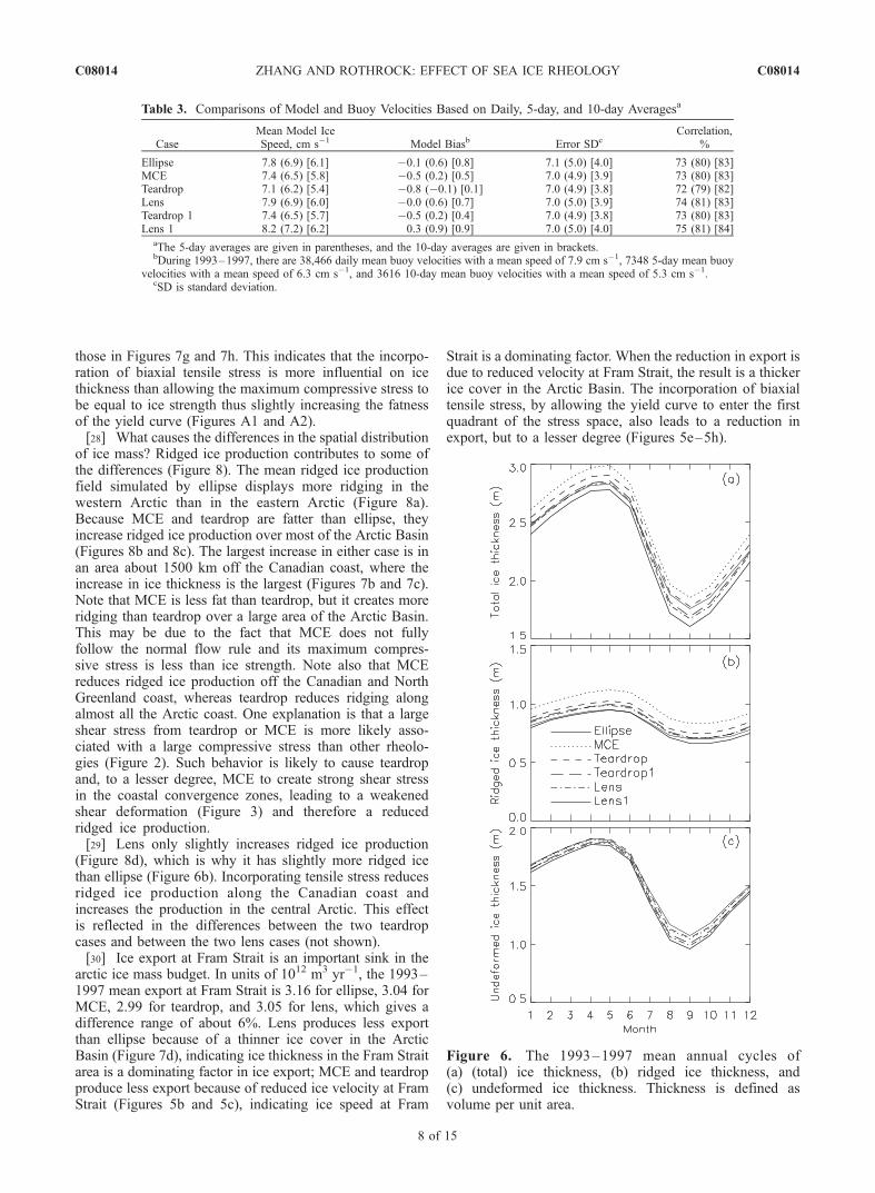
[26] Figure 6a shows annual cycles of ice thicknessaveraged over the Arctic Basin. The 1993–1997 mean icethickness from MCE is noticeably larger than those fromother cases. This is because MCE has significantly moreridged ice (Figure 6b), while the reduction in undeformedice is relatively small in comparison with ellipse (Figure 6c).The ice thickness for teardrop is only slightly larger thanthat for ellipse because the increase in ridged ice thicknessis smaller than for MCE. Teardrop 1 and the two lensrheology cases, on the other hand, produce less ice thanellipse; these cases produce a relatively large reduction inundeformed ice.[27] The mean and difference fields of ice thickness are

plotted in Figure 7. The pattern of the thickness fieldsimulated with ellipse (Figure 7a) agrees reasonably wellwith that observed by Bourke and McLaren [1992]. This is apattern of thicker ice off the Canadian Archipelago andnorth Greenland coast and thinner ice in the eastern Arctic.Compared to ellipse, MCE (Figure 7b) causes ice thicknessto increase considerably over most of the Arctic Basin, up to0.6 m. The increase in ice thickness caused by teardrop ismore limited to the Eurasian Basin, Laptev and Kara seas,and the area a certain distance away from the CanadianArchipelago; it results in less ice in most of the Chukchi andBeaufort seas (Figure 7c). Particularly, ice is reduced alongthe Alaskan and Canadian Archipelago coasts. This is asignificant spatial redistribution of ice mass, relative to

Figure 3. Distributions of simulated (a) shear stress and(b) shear deformation calculated from daily model resultsduring 1993–1997.

Figure 4. Seasonal distributions of simulated shear stresscalculated from daily model results during 1993–1997.


6 of 15

C08014

ellipse. Lens, on the other hand, creates a bit more ice offthe Canadian Archipelago and north Greenland coast and abit less ice over other areas (Figure 7d). The thicknessdifference in the GIN Sea is closely linked to the effect on

ice export at Fram Strait. In addition, allowing biaxialtensile stress tends to increase ice thickness over most ofthe Arctic Basin (Figures 7e–7h). The basic features of thethickness difference fields in Figures 7e and 7f are similar to

Figure 5. The 1993–1997 (a) mean ice velocity and (b–h) difference fields. One vector is drawn forevery nine grid cells. Note the different vector scales in different panels.


7 of 15

C08014

those in Figures 7g and 7h. This indicates that the incorpo-ration of biaxial tensile stress is more influential on icethickness than allowing the maximum compressive stress tobe equal to ice strength thus slightly increasing the fatnessof the yield curve (Figures A1 and A2).[28] What causes the differences in the spatial distribution

of ice mass? Ridged ice production contributes to some ofthe differences (Figure 8). The mean ridged ice productionfield simulated by ellipse displays more ridging in thewestern Arctic than in the eastern Arctic (Figure 8a).Because MCE and teardrop are fatter than ellipse, theyincrease ridged ice production over most of the Arctic Basin(Figures 8b and 8c). The largest increase in either case is inan area about 1500 km off the Canadian coast, where theincrease in ice thickness is the largest (Figures 7b and 7c).Note that MCE is less fat than teardrop, but it creates moreridging than teardrop over a large area of the Arctic Basin.This may be due to the fact that MCE does not fullyfollow the normal flow rule and its maximum compres-sive stress is less than ice strength. Note also that MCEreduces ridged ice production off the Canadian and NorthGreenland coast, whereas teardrop reduces ridging alongalmost all the Arctic coast. One explanation is that a largeshear stress from teardrop or MCE is more likely asso-ciated with a large compressive stress than other rheolo-gies (Figure 2). Such behavior is likely to cause teardropand, to a lesser degree, MCE to create strong shear stressin the coastal convergence zones, leading to a weakenedshear deformation (Figure 3) and therefore a reducedridged ice production.[29] Lens only slightly increases ridged ice production

(Figure 8d), which is why it has slightly more ridged icethan ellipse (Figure 6b). Incorporating tensile stress reducesridged ice production along the Canadian coast andincreases the production in the central Arctic. This effectis reflected in the differences between the two teardropcases and between the two lens cases (not shown).[30] Ice export at Fram Strait is an important sink in the

arctic ice mass budget. In units of 1012 m3 yr�1, the 1993–1997 mean export at Fram Strait is 3.16 for ellipse, 3.04 forMCE, 2.99 for teardrop, and 3.05 for lens, which gives adifference range of about 6%. Lens produces less exportthan ellipse because of a thinner ice cover in the ArcticBasin (Figure 7d), indicating ice thickness in the Fram Straitarea is a dominating factor in ice export; MCE and teardropproduce less export because of reduced ice velocity at FramStrait (Figures 5b and 5c), indicating ice speed at Fram

Strait is a dominating factor. When the reduction in export isdue to reduced velocity at Fram Strait, the result is a thickerice cover in the Arctic Basin. The incorporation of biaxialtensile stress, by allowing the yield curve to enter the firstquadrant of the stress space, also leads to a reduction inexport, but to a lesser degree (Figures 5e–5h).

Table 3. Comparisons of Model and Buoy Velocities Based on Daily, 5-day, and 10-day Averagesa

CaseMean Model IceSpeed, cm s�1 Model Biasb Error SDc

Correlation,%

Ellipse 7.8 (6.9) [6.1] �0.1 (0.6) [0.8] 7.1 (5.0) [4.0] 73 (80) [83]MCE 7.4 (6.5) [5.8] �0.5 (0.2) [0.5] 7.0 (4.9) [3.9] 73 (80) [83]Teardrop 7.1 (6.2) [5.4] �0.8 (�0.1) [0.1] 7.0 (4.9) [3.8] 72 (79) [82]Lens 7.9 (6.9) [6.0] �0.0 (0.6) [0.7] 7.0 (5.0) [3.9] 74 (81) [83]Teardrop 1 7.4 (6.5) [5.7] �0.5 (0.2) [0.4] 7.0 (4.9) [3.8] 73 (80) [83]Lens 1 8.2 (7.2) [6.2] 0.3 (0.9) [0.9] 7.0 (5.0) [4.0] 75 (81) [84]

aThe 5-day averages are given in parentheses, and the 10-day averages are given in brackets.bDuring 1993–1997, there are 38,466 daily mean buoy velocities with a mean speed of 7.9 cm s�1, 7348 5-day mean buoy

velocities with a mean speed of 6.3 cm s�1, and 3616 10-day mean buoy velocities with a mean speed of 5.3 cm s�1.cSD is standard deviation.

Figure 6. The 1993–1997 mean annual cycles of(a) (total) ice thickness, (b) ridged ice thickness, and(c) undeformed ice thickness. Thickness is defined asvolume per unit area.


8 of 15

C08014

4.4. Comparison With Submarine Ice Draft

[31] We compared the model ice draft (simulated icethickness multiplied by 0.89) with submarine observationsof ice draft. The observations, with an uncertainty of about

0.15 m, were acquired by four submarine cruises from 1993to 1997 (Figure 9). They were compared with model draftssampled at the location of each dot at the correspondingtime (Table 4 and Figure 9). Given the dynamical and

Figure 7. The 1993–1997 (a) mean ice thickness and (b–h) difference fields. The contour interval is0.5 m for the mean field and 0.05 m for the difference fields.


9 of 15

C08014

thermodynamical forcing and model parameterization,MCE and lens 1 have relatively higher bias in meanice draft along the submarine tracks. The difference in thedraft between MCE and the lens 1 is 0.30 m, or 16%.The lens rheologies generally perform worse than theteardrop rheologies. Lens 1, in particular, has relativelylow correlation and high bias and error standard deviation(SD).[32] Moderately, teardrop appears to have the best overall

performance in obtaining the highest correlation and thelowest bias and error SD. This indicates that the spatialdifference in ice mass as seen in Figure 7c helps improvemodel agreement with observations. As shown in Figure 9a,ellipse tends to overestimate ice draft in the Beaufort Seaand underestimate ice draft in the Eurasian Basin and nearthe North Pole for 1993–1997. A careful examinationreveals that, to a varying degree, teardrop tends to reducesuch model bias in all these areas (Figures 9c and 10). MCEis also able to somewhat reduce model bias in the EurasianBasin and North Pole area, but not in the Beaufort Sea. Inaddition, it tends to create more large overestimates thanother rheologies (Figure 10). In comparison with ellipse, thetwo lens rheologies actually enlarge the spatial model biasslightly (Figure 9d). It consistently underestimates ice draftsuch that its distribution of model-data difference in icedraft peaks at �0.6 m (Figure 10).

4.5. Surface Energy Exchanges

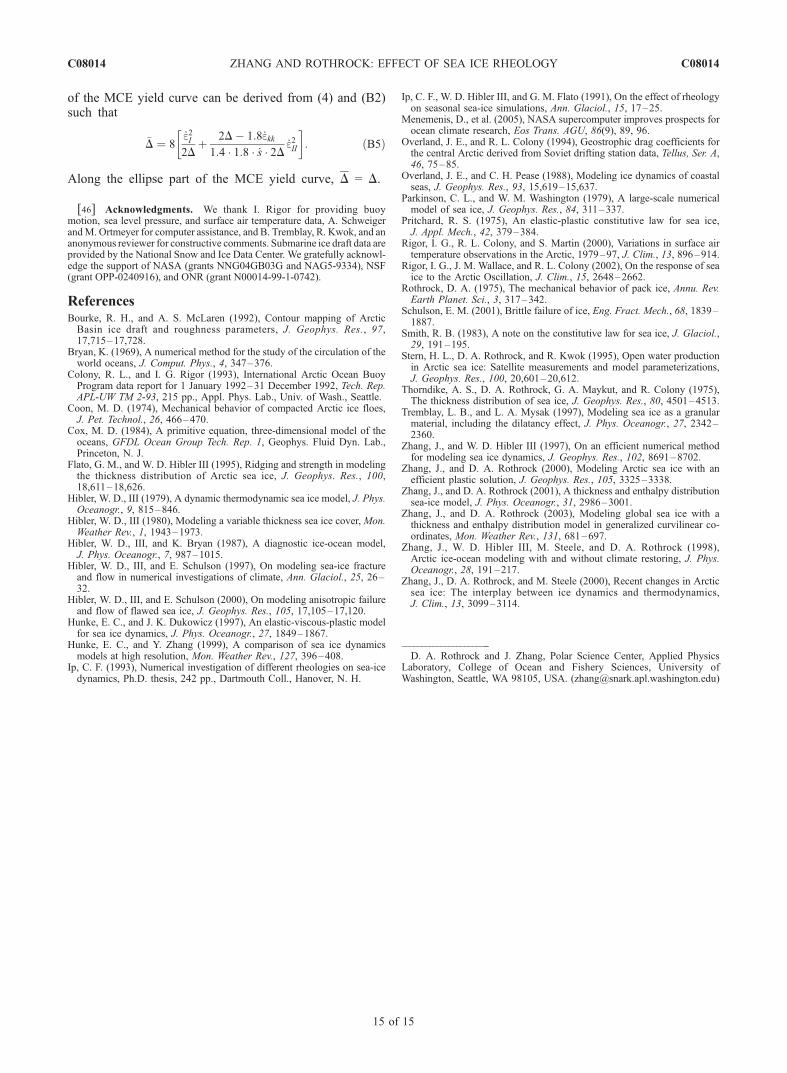
[33] To what degree does sea ice rheology affect thesurface energy exchange in climate models? To address thisquestion, we plotted the 1993–1997 mean and difference

fields of upward net surface heat flux (Figure 11). Thedifferences in the surface heat loss are generally less than0.5 Wm�2 in the central Arctic. The differences in theaveraged values over the entire ice covered areas are alsowithin 0.5 W m�2, with the average being 9.2 W m�2 forellipse, teardrop, and lens, and 9.6 W m�2 for MCE. How-ever, locally differences can reach 3 W m�2 in the Arcticmarginal seas, such as the East Siberian and Laptev seas, andin some coastal areas. Outside the Arctic Basin, mainly in themarginal ice zones in the Barents and GIN seas, the differ-ences are much larger, up to 8 W m�2 (Figures 11 and 12),owing to differences in surface conditions such as ice cover-age and thickness. The average surface heat loss over areascovered by ice thinner than 1 m is 32 W m�2 for ellipse andteardrop, 34Wm�2 forMCE, and 33Wm�2 for lens. That is,the difference between MCE and ellipse is 6%. In addition,the areas with a difference of 3Wm�2 ormore consist of up to10% of the entire ice covered areas and 27% of the areascovered by ice thinner than 1 m (Figure 12). This is also truefor the components of the surface heat flux: net shortwave andlongwave radiative fluxes and net sensible and latent heatfluxes (not shown). This indicates that sea ice rheology, bychanging ice motion, deformation, and thickness, has asignificant impact on the calculation of the surface energybudget, particularly in long-termmodeling of climate change.

5. Concluding Remarks

[34] We have developed mathematical formulations forsea ice constitutive laws that employ teardrop and paraboliclens plastic yield curves. Like the widely used ellipse

Figure 8. The 1993–1997 (a) mean ridged ice production and (b–d) difference fields. The contourinterval is 0.2 m yr�1 for the mean field and 0.05 m yr�1 for the difference fields.


10 of 15

C08014

rheology [Hibler, 1979], they are isotropic plastic rheolo-gies that obey the normal flow rule when ice fails; like theMCE rheology [Hibler and Schulson, 2000], they follow thelaboratory observations of ice mechanical property byallowing varying amount of biaxial tensile stress. In orderto examine the effects of a plastic rheology in numericalinvestigations of climate, the teardrop and lens rheologies,together with the ellipse and the MCE rheologies, werenumerically implemented in a thickness and enthalpy dis-tribution ice model for the Arctic, Barents, and GIN seas.Reasonably good viscous-plastic solutions are achievedusing each rheology, with about 90% of ice internal stressesfalling either on or inside the yield curves (Figure 2).[35] Model results from a series of integrations indicate

that plastic rheology has a significant effect on large-scalesea ice simulations. For the whole simulation period of1993–1997, rheologies that fully follow the normal flowrule have shear stress distributions with two peaks, one atthe zero shear stress and the second between 16,000–30,000 N m�1. The second peak is around 16,000 N m�1

for the ellipse and two lens rheologies and around30,000 N m�1 for the two teardrop rheologies. On thebasis of Coulombic friction failure and only partiallyobeying the normal flow rule, the MCE rheology createsa shear stress distribution without a second peak. This isbecause MCE usually does not tend to create a secondpeak in spring and fall, an interesting distinction revealedby model results.

Figure 9. Modeled minus observed ice draft (m) along submarine cruise tracks from 1993 to 1997. Dotsillustrate available observations of ice draft collected along four tracks of submarine cruises in September1993, April 1994, September 1996, and September–October 1997. Each dot in the plot represents arecord of ice thickness averaged over a distance of �10–50 km along the tracks.

Table 4. Modeled and Observed Ice Drafts Compared Along

Tracks of Four Submarine Cruises in 1993–1997a

CaseMean ModelDraft, m Bias Error SD Correlation

Ellipse 2.01 0.04 0.71 0.44MCE 2.13 0.16 0.75 0.47Teardrop 2.01 0.04 0.69 0.51Lens 1.91 �0.06 0.73 0.45Teardrop 1 1.90 �0.07 0.69 0.50Lens 1 1.83 �0.14 0.74 0.42

aThere are 639 observed drafts with a mean of 1.97 m.


11 of 15

C08014

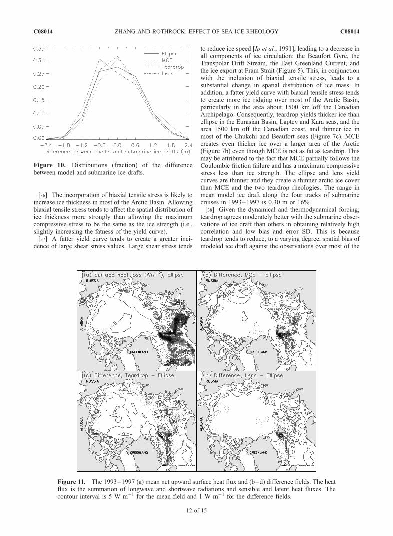
[36] The incorporation of biaxial tensile stress is likely toincrease ice thickness in most of the Arctic Basin. Allowingbiaxial tensile stress tends to affect the spatial distribution ofice thickness more strongly than allowing the maximumcompressive stress to be the same as the ice strength (i.e.,slightly increasing the fatness of the yield curve).[37] A fatter yield curve tends to create a greater inci-

dence of large shear stress values. Large shear stress tends

to reduce ice speed [Ip et al., 1991], leading to a decrease inall components of ice circulation: the Beaufort Gyre, theTranspolar Drift Stream, the East Greenland Current, andthe ice export at Fram Strait (Figure 5). This, in conjunctionwith the inclusion of biaxial tensile stress, leads to asubstantial change in spatial distribution of ice mass. Inaddition, a fatter yield curve with biaxial tensile stress tendsto create more ice ridging over most of the Arctic Basin,particularly in the area about 1500 km off the CanadianArchipelago. Consequently, teardrop yields thicker ice thanellipse in the Eurasian Basin, Laptev and Kara seas, and thearea 1500 km off the Canadian coast, and thinner ice inmost of the Chukchi and Beaufort seas (Figure 7c). MCEcreates even thicker ice over a larger area of the Arctic(Figure 7b) even though MCE is not as fat as teardrop. Thismay be attributed to the fact that MCE partially follows theCoulombic friction failure and has a maximum compressivestress less than ice strength. The ellipse and lens yieldcurves are thinner and they create a thinner arctic ice coverthan MCE and the two teardrop rheologies. The range inmean model ice draft along the four tracks of submarinecruises in 1993–1997 is 0.30 m or 16%.[38] Given the dynamical and thermodynamical forcing,

teardrop agrees moderately better with the submarine obser-vations of ice draft than others in obtaining relatively highcorrelation and low bias and error SD. This is becauseteardrop tends to reduce, to a varying degree, spatial bias ofmodeled ice draft against the observations over most of the

Figure 10. Distributions (fraction) of the differencebetween model and submarine ice drafts.

Figure 11. The 1993–1997 (a) mean net upward surface heat flux and (b–d) difference fields. The heatflux is the summation of longwave and shortwave radiations and sensible and latent heat fluxes. Thecontour interval is 5 W m�1 for the mean field and 1 W m�1 for the difference fields.


12 of 15

C08014

areas covered by 1993–1997 submarine cruises. Teardrop isalso found to reduce ice thickness along the coastal con-vergence/shear zones, which contributes to the reduction ofmodel bias in the Beaufort Sea.[39] The results also indicate that plastic rheology, which

changes the model’s solution of ice motion, deformation,and thickness, has a significant impact on the computationof surface energy exchanges. Although the local differencesin surface heat fluxes among all the rheology cases aregenerally less than 0.5 W m�2 in the central Arctic, they canbe as high as 3 W m�2 in the Arctic marginal seas and ashigh as 8 W m�2 in the marginal ice zones in the Barentsand GIN seas. Among the thin ice areas where greatersurface exchanges occur, the percentage of the areas with adifference of 3 W m�2 or more can reach 27%. In a coupledclimate model with atmosphere, ocean, and sea ice compo-nents, such differences would likely have a significantimpact on the overall energy budget of the model.[40] A variety of rheologies have been compared; all are

isotropic rheologies that can be integrated easily in climatemodels. Although varying in performance, they all simulatereasonably realistic ice motion and thickness compared withbuoy and submarine observations. These rheologies open upanother dimension for model calibration and adjustment, inaddition to traditional tuning of some model parameterssuch as air drag and ice strength. What rheology should wechoose for climate modeling? The ellipse has been widelyused and resulted in realistic results, but the MCE, teardrop,

and lens are all equipped with biaxial tensile stress that is inline with lab experiments. Teardrop is generally preferredbecause of its improved agreement with ice draft observa-tions. However, this assessment is based on only one study.Whether teardrop is better in other applications needs to beexamined.

Appendix A: Derivation of Constitutive LawsWith Teardrop and Lens Yield Curves

[41] In a normalized stress space (Figure A1), bothteardrop and lens plastic yield curves can be described bya common equation

sII=P ¼ � sI=P � að Þ 1þ aþ sI=P � að Þ½ �q; ðA1Þ

where a is the biaxial tensile stress parameter, q is thefatness factor determining the shape of the curve (q = 1/2 forteardrop and q = 1 for parabolic lens), and sI and sII aredefined as

sI ¼1

2s1 þ s2ð Þ and sII ¼

1

2s1 � s2ð Þ; ðA2Þ

where s1 and s2 are the principal stresses. If _eI and _eII aresimilarly defined in terms of principal strain rates _e1 and _e2,the relationship between stress and strain rate described by(2) can be written as

sI ¼ 2V_eI � P=2 and sII ¼ 2h_eII : ðA3Þ

A1. Constitutive Law With a Teardrop Yield Curve

[42] Squaring both sides of (A1) with a fatness factorof q = 1/2 and applying the normal flow rule gives

@F

@u¼ g_eI and

@F

@y¼ g_eII ; ðA4Þ

where

u ¼ x� a; x ¼ sI=P; y ¼ sII=P ¼ � x� að Þ 1þ xð Þ1=2; ðA5Þ

F ¼ y2 � 1þ að Þu2 � u3 ¼ 0: ðA6Þ

Figure 12. Distributions (fraction) of the difference in netsurface heat flux for 1993–1997 (a) over ice-covered areasand (b) over areas covered by ice thinner than 1 m.

Figure A1. Teardrop and lens yield curves in a sI � sIIcoordinate system, with the maximum compressive stressindependent of the maximum tensile stress (for teardrop andlens rheologies).


13 of 15

C08014

From (A4) and (A6) we get, after some algebra, thefollowing equation

9u2 þ 12 1þ að Þ � 4k2� �

uþ 4 1þ að Þ2�4k2 1þ að Þh i

¼ 0;

ðA7Þ

where k = _eI/_eII. For k � 1 the solution for (A7) is

u ¼ � 6 1þ að Þ � 2k2½ � þ 2kffiffiffiffiffiffiffiffiffiffiffiffiffiffiffiffiffiffiffiffiffiffiffiffiffiffiffik2 þ 3 1þ að Þ

p9

: ðA8Þ

Once u is determined, x and y are determined by (A5). Fork > 1, we set x = a and y = 0. The viscosities can be derivedfrom (A3) and (A5) such that

V ¼ sI þ P=2

2_eI¼ xþ 1=2

2_eIP; ðA9Þ

h ¼ sII2_eII

¼ y

2_eIIP ¼ � x� að Þ 1þ xð Þ1=2

2_eIIP: ðA10Þ

A2. Constitutive Law With a Parabolic Lens YieldCurve

[43] We similarly apply the normal flow rule on (A2) witha fatness factor of q = 1 and with

F ¼ yþ u 1þ aþ uð Þ ¼ 0: ðA11Þ

For jkj � 1 the solution for (A4) and (A11) is

u ¼ k � 1� að Þ=2: ðA12Þ

Once u is determined we have

x ¼ sI=P ¼ uþ a and y ¼ sII=P ¼ � x� að Þ 1þ xð Þ: ðA13Þ

Also, we set x = a, y = 0 for k > 1, and x = –1, y = 0for k < –1. The viscosities are

V ¼ sI þ P=2

2_eI¼ xþ 1=2

2_eIP; ðA14Þ

h ¼ sII2_eII

¼ y

2_eIIP ¼ � x� að Þ 1þ xð Þ

2_eIIP: ðA15Þ

What is the best choice for the biaxial tensile stressparameter a is not clear. In this study, however, thebiaxial tensile stress parameter a is set to 0.05 for eitherteardrop or lens rheology, which allows biaxial tensilestress comparable to that allowed by the MCE rheology(Figure 1). Setting a = 0, we obtain the teardrop 1 orlens 1 rheology that does not allow any tensile stress.[44] Note that, in addition to allowing biaxial tensile

stress, teardrop and lens yield curves are also fatter thanteardrop 1 and lens 1. In order to single out the effect ofincorporating biaxial tensile stress, teardrop 2 and lens 2(section 3) have been used also for model integrations.Teardrop 2 and lens 2 have the same fatness as teardrop 1and lens 1, while allowing biaxial tensile stress. A commonequation parallel to (A1) for describing teardrop 2 and lens2 plastic yield curves (Figure A2) can be written as

sII=P ¼ � sI=P � að Þ 1þ sI=P � að Þ½ �q:

The solutions can be similarly derived to be

u ¼ � 6� 2k2ð Þ þ 2kffiffiffiffiffiffiffiffiffiffiffiffiffik2 þ 3

p

9

for teardrop 2, and

u ¼ k � 1ð Þ=2

for lens 2.

Appendix B: Derivation of the NormalizedMechanical Energy Dissipation Rate

[45] The normalized mechanical energy dissipation rateM described in (9) is determined once the D function isdetermined. From (A2) and with a 45 rotation of theprincipal stresses, the total normalized energy dissipationrate can be written as

P�1sij _eij ¼ P�1si _ei ¼ 2P�1 sI _eI þ sII _eIIð Þ: ðB1Þ

Applying (10) and (A3) leads to

P�1sij _eij ¼ 4 V_e2I þ h_e2II� �

=P � _eI ¼1

2�D� _ekk

� �; ðB2Þ

where D = 8(V_eI2 + h_eII

2 )/P. From (A9), (A10), (A14), (A15),and (B2) we obtain

�D ¼ 4 xþ 1=2ð Þ_eI � x� að Þ 1þ xð Þ1=2 _eIIh i

ðB3Þ

for the teardrop rheologies (teardrop and teardrop 1) and

�D ¼ 4 xþ 1=2ð Þ_eI � x� að Þ 1þ xð Þ _eII½ � ðB4Þ

for the lens rheologies (lens and lens 1). Similarprocedures can be applied for teardrop 2 and lens 2.The corresponding equation for the Mohr-Coulomb part

Figure A2. Teardrop and lens yield curves in a sI � sIIcoordinate system, with the maximum compressive stressdepending on the maximum tensile stress (for teardrop 2and lens 2 rheologies).


14 of 15

C08014

of the MCE yield curve can be derived from (4) and (B2)such that

�D ¼ 8_e2I2D

þ 2D� 1:8_ekk1:4 � 1:8 � _s � 2D

_e2II

� �: ðB5Þ

Along the ellipse part of the MCE yield curve, D = D.

[46] Acknowledgments. We thank I. Rigor for providing buoymotion, sea level pressure, and surface air temperature data, A. SchweigerandM. Ortmeyer for computer assistance, and B. Tremblay, R. Kwok, and ananonymous reviewer for constructive comments. Submarine ice draft data areprovided by the National Snow and Ice Data Center. We gratefully acknowl-edge the support of NASA (grants NNG04GB03G and NAG5-9334), NSF(grant OPP-0240916), and ONR (grant N00014-99-1-0742).

ReferencesBourke, R. H., and A. S. McLaren (1992), Contour mapping of ArcticBasin ice draft and roughness parameters, J. Geophys. Res., 97,17,715–17,728.

Bryan, K. (1969), A numerical method for the study of the circulation of theworld oceans, J. Comput. Phys., 4, 347–376.

Colony, R. L., and I. G. Rigor (1993), International Arctic Ocean BuoyProgram data report for 1 January 1992–31 December 1992, Tech. Rep.APL-UW TM 2-93, 215 pp., Appl. Phys. Lab., Univ. of Wash., Seattle.

Coon, M. D. (1974), Mechanical behavior of compacted Arctic ice floes,J. Pet. Technol., 26, 466–470.

Cox, M. D. (1984), A primitive equation, three-dimensional model of theoceans, GFDL Ocean Group Tech. Rep. 1, Geophys. Fluid Dyn. Lab.,Princeton, N. J.

Flato, G. M., and W. D. Hibler III (1995), Ridging and strength in modelingthe thickness distribution of Arctic sea ice, J. Geophys. Res., 100,18,611–18,626.

Hibler, W. D., III (1979), A dynamic thermodynamic sea ice model, J. Phys.Oceanogr., 9, 815–846.

Hibler, W. D., III (1980), Modeling a variable thickness sea ice cover, Mon.Weather Rev., 1, 1943–1973.

Hibler, W. D., III, and K. Bryan (1987), A diagnostic ice-ocean model,J. Phys. Oceanogr., 7, 987–1015.

Hibler, W. D., III, and E. Schulson (1997), On modeling sea-ice fractureand flow in numerical investigations of climate, Ann. Glaciol., 25, 26–32.

Hibler, W. D., III, and E. Schulson (2000), On modeling anisotropic failureand flow of flawed sea ice, J. Geophys. Res., 105, 17,105–17,120.

Hunke, E. C., and J. K. Dukowicz (1997), An elastic-viscous-plastic modelfor sea ice dynamics, J. Phys. Oceanogr., 27, 1849–1867.

Hunke, E. C., and Y. Zhang (1999), A comparison of sea ice dynamicsmodels at high resolution, Mon. Weather Rev., 127, 396–408.

Ip, C. F. (1993), Numerical investigation of different rheologies on sea-icedynamics, Ph.D. thesis, 242 pp., Dartmouth Coll., Hanover, N. H.

Ip, C. F., W. D. Hibler III, and G. M. Flato (1991), On the effect of rheologyon seasonal sea-ice simulations, Ann. Glaciol., 15, 17–25.

Menemenis, D., et al. (2005), NASA supercomputer improves prospects forocean climate research, Eos Trans. AGU, 86(9), 89, 96.

Overland, J. E., and R. L. Colony (1994), Geostrophic drag coefficients forthe central Arctic derived from Soviet drifting station data, Tellus, Ser. A,46, 75–85.

Overland, J. E., and C. H. Pease (1988), Modeling ice dynamics of coastalseas, J. Geophys. Res., 93, 15,619–15,637.

Parkinson, C. L., and W. M. Washington (1979), A large-scale numericalmodel of sea ice, J. Geophys. Res., 84, 311–337.

Pritchard, R. S. (1975), An elastic-plastic constitutive law for sea ice,J. Appl. Mech., 42, 379–384.

Rigor, I. G., R. L. Colony, and S. Martin (2000), Variations in surface airtemperature observations in the Arctic, 1979–97, J. Clim., 13, 896–914.

Rigor, I. G., J. M. Wallace, and R. L. Colony (2002), On the response of seaice to the Arctic Oscillation, J. Clim., 15, 2648–2662.

Rothrock, D. A. (1975), The mechanical behavior of pack ice, Annu. Rev.Earth Planet. Sci., 3, 317–342.

Schulson, E. M. (2001), Brittle failure of ice, Eng. Fract. Mech., 68, 1839–1887.

Smith, R. B. (1983), A note on the constitutive law for sea ice, J. Glaciol.,29, 191–195.

Stern, H. L., D. A. Rothrock, and R. Kwok (1995), Open water productionin Arctic sea ice: Satellite measurements and model parameterizations,J. Geophys. Res., 100, 20,601–20,612.

Thorndike, A. S., D. A. Rothrock, G. A. Maykut, and R. Colony (1975),The thickness distribution of sea ice, J. Geophys. Res., 80, 4501–4513.

Tremblay, L. B., and L. A. Mysak (1997), Modeling sea ice as a granularmaterial, including the dilatancy effect, J. Phys. Oceanogr., 27, 2342–2360.

Zhang, J., and W. D. Hibler III (1997), On an efficient numerical methodfor modeling sea ice dynamics, J. Geophys. Res., 102, 8691–8702.

Zhang, J., and D. A. Rothrock (2000), Modeling Arctic sea ice with anefficient plastic solution, J. Geophys. Res., 105, 3325–3338.

Zhang, J., and D. A. Rothrock (2001), A thickness and enthalpy distributionsea-ice model, J. Phys. Oceanogr., 31, 2986–3001.

Zhang, J., and D. A. Rothrock (2003), Modeling global sea ice with athickness and enthalpy distribution model in generalized curvilinear co-ordinates, Mon. Weather Rev., 131, 681–697.

Zhang, J., W. D. Hibler III, M. Steele, and D. A. Rothrock (1998),Arctic ice-ocean modeling with and without climate restoring, J. Phys.Oceanogr., 28, 191–217.

Zhang, J., D. A. Rothrock, and M. Steele (2000), Recent changes in Arcticsea ice: The interplay between ice dynamics and thermodynamics,J. Clim., 13, 3099–3114.

��D. A. Rothrock and J. Zhang, Polar Science Center, Applied Physics

Laboratory, College of Ocean and Fishery Sciences, University ofWashington, Seattle, WA 98105, USA. ([email protected])


15 of 15

C08014

Documents

Effect of sea ice rheology in numerical investigations of climate