Effect of replenishment and backroom on retail shelf-space

ORIGINAL RESEARCH

Effect of replenishment and backroom on retailshelf-space planning

Alexander Hubner1• Kai Schaal1

Received: 16 March 2016 /Accepted: 8 December 2016 / Published online: 9 January 2017

� The Author(s) 2017. This article is published with open access at Springerlink.com

Abstract Shelf-space optimization models support retailers in making optimal

shelf-space decisions. They determine the number of facings for each item included

in an assortment. One common characteristic of these models is that they do not

account for in-store replenishment processes. However, the two areas of shelf-space

planning and in-store replenishment are strongly interrelated. Keeping more shelf

stock of an item increases the demand for it due to higher visibility, permits

decreased replenishment frequencies and increases inventory holding costs. How-

ever, because space is limited, it also requires the reduction of shelf space for other

items, which then deplete faster and must be reordered and replenished more often.

Furthermore, the possibility of keeping stock of certain items in the backroom

instead of the showroom allows for more showroom shelf space for other items, but

also generates additional replenishment costs for the items kept in the backroom.

The joint optimization of both shelf-space decisions and replenishment processes

has not been sufficiently addressed in the existing literature. To quantify the cost

associated with the relevant in-store replenishment processes, we conducted a time

and motion study for a German grocery retailer. Based on these insights, we propose

an optimization model that addresses the mutual dependence of shelf-space deci-

sions and replenishment processes. The model optimizes retail profits by deter-

mining the optimum number of facings, the optimum display orientation of items,

and the optimum order frequencies, while accounting for space-elasticity effects as

well as limited shelf and backroom space. Applying our model to the grocery

retailer’s canned foods category, we found a profit potential of about 29%. We

further apply our model to randomly generated data and show that it can be solved

to optimality within very short run times, even for large-scale problem instances.

Finally, we use the model to show the impact of backroom space availability and

& Alexander Hubner

[email protected]

1 Catholic University Eichstaett-Ingolstadt, Ingolstadt, Germany

123

Business Research (2017) 10:123–156

DOI 10.1007/s40685-016-0043-6

http://orcid.org/0000-0002-1358-1284

http://crossmark.crossref.org/dialog/?doi=10.1007/s40685-016-0043-6&domain=pdf

http://crossmark.crossref.org/dialog/?doi=10.1007/s40685-016-0043-6&domain=pdf

replenishment cost on retail profits and solution structures. Based on the insights

gained from the application of our model, the grocery retailer has decided to change

its current approach to shelf-space decisions and in-store replenishment planning.

Keywords Shelf space � Backroom � Space-elastic demand � Optimization �Replenishment

1 Introduction

Retailers use shelves to offer their products to customers. In doing so, they must

decide how much shelf space to allocate to which item. Because shelf quantities

assigned to retail shelves become depleted over time due to customer purchases,

retailers need to regularly refill shelves and reorder items. Reordering directly

impacts replenishment processes. As soon as reorders arrive at the store, the

respective items are transported to the showroom, where shelves are replenished

(i.e., direct replenishment). As a result, every order process triggers a direct

replenishment process. Items that do not fit onto the showroom shelf space are

stored in the backroom, from where shelves are later replenished (i.e., indirect

replenishment from backroom).

Both decisions, i.e., shelf space and reordering, are interrelated, because, e.g., to

meet customer demand, a retailer has the option of increasing the shelf quantity and

decreasing the order frequency for a specific item, or vice versa. If space is limited,

a higher shelf quantity for one item implies less frequent reorders and replenish-

ments for this item, but also less space available for other items, which in turn must

be reordered more frequently.

Shelf-space and reorder planning are of great importance to retailers for several

reasons: The increasing number of products is in conflict with limited shelf space.

Today, up to 30% more products than ten years ago compete for scare space (EHI

Retail Institute 2014; Hubner et al. 2016). This puts retailers under pressure to

manage profitability with narrow margins and to maintain space productivity

(Gutgeld et al. 2009). In fact, shelf space has been referred to as a retailer’s scarcest

resource (cf. e.g., Lim et al. 2004; Irion et al. 2012; Geismar et al. 2015; Bianchi-

Aguiar et al. 2015a). Above all, changes in shelf space impact customer demand

due to the higher visibility of items (Eisend 2014). In other words, the demand for

an item grows, the more shelf space is allocated to it. This is referred to as ‘‘space-

elastic demand’’. Additionally, the costs associated with in-store replenishment are

significant, because in-store logistics costs amount to up to 50% of total retail

supply chain costs (Kotzab and Teller 2005; Broekmeulen et al. 2006; Reiner et al.

2013; Kuhn and Sternbeck 2013). However, the options for changing replenishment

frequencies are subject to the availability of backroom inventory for intermediate

storage (Eroglu et al. 2013; Pires et al. 2016) and the degree of freedom to choose

different delivery frequencies (Sternbeck and Kuhn 2014). Besides product margins

and demand effects, the shelf-space planner should therefore also consider options

for arranging items on the shelf, in-store replenishment frequencies and costs, and

the availability of a backroom for replenishment.

124 Business Research (2017) 10:123–156

123

Current literature on shelf-space management mainly addresses the demand side

by modeling the effect of space-elastic demand. In this case, a retailer’s profit is

maximized under shelf-space constraints by defining the number of facings for each

product (i.e., first visible unit of an item in the front row; Hubner and Kuhn 2012;

Kok et al. 2015). Existing models do not account for replenishment frequencies and

costs, or options for leveraging backroom inventory (Hubner and Kuhn 2012;

Bianchi-Aguiar et al. 2016).

To investigate the above-mentioned relationships, we conducted a time and

motion study for a German grocery retailer and identified both the relevant in-store

replenishment processes and the associated costs. Building on these insights, we

then develop an optimization model that simultaneously optimizes shelf-space and

in-store replenishment decisions while also accounting for space-elastic demand as

well as limited showroom and backroom space. The model accounts not only for

product margins, but also for the costs of direct shelf replenishment upon delivery of

orders to the store, and for replenishment from the backroom. Furthermore, we

consider the cost of inventory kept in the showroom and the backroom. This

extended model addresses the research question of how different replenishment

procedures and the opportunity to use backroom space impact shelf-space planning.

We apply the model to show why an integrated perspective on shelf-space and in-

store replenishment optimization is worthwhile and demonstrate how retailers can

apply the model to increase their profits.

We address the trade-offs between shelf-space allocation and in-store replenish-

ment (e.g., more space, less frequent orders and replenishments). Because retailers

use backrooms as a planned buffer or for excess inventory after shelf replenishment,

we further investigate how the availability of a backroom impacts shelf-space

decisions and order frequencies.

The remainder of this paper is organized as follows: Sect. 2 provides the

conceptual background of our paper and presents the related literature on shelf-

space optimization. The time and motion study, and the description of identified

replenishment processes, are presented in Sect. 3. Section 4 explains the optimiza-

tion model and presents a solution approach. Numerical results for testing our model

and the impact of backroom space and replenishment cost on objective values and

solution structures are presented in Sect. 5. Finally, Sect. 6 has the conclusion and

outlook.

2 Conceptual background and related literature

2.1 Conceptual background and decision problem

In the following, we analyze the basic decisions retailers need to make in shelf-

space and reorder planning, namely (1) how much shelf space to allocate to items,

and (2) how often to reorder them.

(1) Shelf-space decision Shelf-space planning is a mid-term task and typically

executed every six months, requiring a retailer to assign shelf space and shelf

quantities to listed products under the constraints of limited shelf size (Hubner and

Business Research (2017) 10:123–156 125

123

Kuhn 2012; Hubner et al. 2013; Bianchi-Aguiar et al. 2016). The results of these

decisions are visualized in a planogram which displays the number of facings,

display orientation and position on the shelf for every item (cf. Fig. 1). A facing is

the first visible unit of an item in the front row of a shelf. Behind each facing, there

is certain quantity of stock, i.e., additional units of the respective item. The number

of facings and the stock per facing determine the total shelf quantity of an item.

Furthermore, items can be displayed lengthwise or crosswise (cf. Dreze et al. 1994).

Particularly when single units of an item are stored in cartons, the retailer must

decide on the display orientation of the respective carton. Figure 1, left, shows the

difference between facings and shelf quantities. For example, item a gets 2 facings

with a stock of 4 units each, resulting in a total quantity of 2 � 4 ¼ 8 units. Item

b gets 1 facing with a stock of 6 units and a total shelf quantity of 6. The right of

Fig. 1 explains the difference between length- and crosswise display orientation.

Display orientation also impacts the stock per facing since more or fewer units of

an item fit behind one facing depending on whether the item is positioned length- or

crosswise. In Fig. 1, fewer units would fit behind one facing lengthwise and more

units behind a facing with crosswise display orientation. The stock that can be

placed behind one facing is determined by the depth of the shelf and the item

dimensions. Since the space behind one facing is always filled completely after a

replenishment (i.e., filled up until the shelf depth is fully occupied), the stock per

facing is not itself a decision of the retailer, but is determined via shelf and item

dimensions as well as the decision on the display orientation.

Finally, the position of an item on the shelf is described by its vertical (i.e., which

shelf level) and horizontal position (i.e., which items are located next to each other).

We focus on the core demand effect of space elasticity, and therefore do not account

for these positioning effects in our model. For models accounting for item

positioning, we refer the reader to e.g., Hwang et al. (2009), Hansen et al. (2010),

Russell and Urban (2010) and Hubner and Schaal (2017).

Shelf-space decisions impact customer demand. Item demand depends on the

visible quantity on the shelf and the display orientation. The higher the visibility of

an item, the higher its demand. The visibility of an item increases with the number

of facings assigned to that item and its display orientation, i.e., the visible item

width the customer sees. Empirical studies examine these so-called ‘‘space-

elasticity effects’’, (cf. e.g., Cox 1964; Frank and Massy 1970; Curhan 1972; Dreze

et al. 1994; Desmet and Renaudin 1998). Chandon et al. (2009) show that the

Fig. 1 Illustration of facing, shelf quantity and display orientation


123

number of facings is the most important in-store factor affecting customer demand.

Using a meta-analysis across empirical studies, Eisend (2014) quantified the average

space-elasticity factor as 17%, which implies a demand increase of 17% each time

the number of facings is doubled. The discussion of the demand effect on other

items (referred to as ‘‘cross-space elasticity’’) is ambiguous in the pertinent

literature. For example, Zufryden (1986) and Kok et al. (2015) state that there is no

empirical evidence that product-level demand can be modeled with cross-space

elasticity. In addition, the measured effects of cross-space elasticity appear to have

only a limited influence on sales (Eisend 2014; Hubner and Schaal 2016). We

therefore comply with these results in the literature and disregard cross-space

elasticity effects in the remainder of our paper.

Furthermore, shelf-space decisions also depend on assortment planning. How-

ever, in retail practice assortment and shelf-space decisions are typically two

sequential planning steps of the category planning process (Hubner et al. 2013; Kok

et al. 2015; Bianchi-Aguiar et al. 2016). Assortment planning is usually executed in

an overarching planning step by the marketing department, whereas shelf planning

is a subordinate planning problem and generally owned by the sales department.

However, if the shelf space planner can also make assortment decisions and delist

items (due to shelf space constraints, for instance, or low profitability of items), one

needs to take into account potential substitutions due to demand switches from

delisted to listed items.

(2) Ordering decision Since ordering decisions impact store operations, thorough

reorder planning is crucial for retailers (see e.g., Fisher 2009; Zelst et al. 2009;

Donselaar et al. 2010; DeHoratius and Zeynep 2015). Kuhn and Sternbeck (2013)

use qualitative interviews to identify that space management and in-store logistics

are not yet well aligned, and that this constitutes a new area of research. Reiner

et al. (2013) identify opportunities for improving in-store logistics and show that it

is important to not only consider customer needs and the demand side when

designing store layout and taking shelf-space decisions, but also logistics

requirements. Their process analysis reveals that the efficient design of in-store

logistics processes leads to substantial service performance improvements.

Furthermore, Kotzab et al. (2005) and Kotzab et al. (2007) use qualitative

interviews with store managers to identify the relevant in-store logistics and

replenishment processes. Their findings and process descriptions form the starting

point of our research.

Because shelves are depleted over time due to customer purchases, retailers need

to reorder items and replenish shelves. Consequently, a retailer needs to decide how

often to reorder an item. This order frequency impacts in-store logistic processes,

because each order triggers a delivery from the warehouse to the store, which again

results in a direct replenishment effort to transport the delivered items to the

showroom shelves. Beyond this, the order frequency also impacts the number of

replenishments from the backroom, because the less frequently items are ordered

from warehouses, the higher the backroom quantity at the store that needs to be kept

if shelf space is not sufficient to fulfill customer demand, and the higher the number

of replenishments of showroom shelves from the backroom. We discuss the in-store


123

logistics processes related to direct and backroom replenishment in more detail in

Sect. 3.

2.2 Related literature on shelf-space optimization

Following Seuring et al. (2005) and Kotzab et al. (2005), we first defined the scope

of our contribution (as in Sect. 2.1), and then identified the related literature. The

identification step included the material collection/selection and category selection.

Finally, we completed a content analysis. Because we focus on quantitative decision

models, we excluded literature that strictly covers general management, marketing

and service management issues, and does not discuss modeling aspects and decision

support systems at all. Papers were assessed based on their decision modeling,

demand models and their relation to space and reorder planning.

In the following we introduce the fundamental modeling papers and analyze only

the shelf-space modeling papers that contain considerations of replenishment,

inventory holding and store operations. Further modeling papers dealing with shelf-

space problems that do not include any of these considerations or that are not related

to our decision problem are not the focus and not further analyzed. Shelf-space

models typically assume a given assortment with space-elastic demand, ignore

substitution (because the assortment is predetermined), and account for limited shelf

space. Our problem relates to the shelf-space literature, and we therefore focus on

this area. For comprehensive overviews of shelf-space problems, we refer to Hubner

and Kuhn (2012), Kok et al. (2015) and Bianchi-Aguiar et al. (2016).

The models reviewed here all optimize the number of facings for a given set of

items and limited shelf space. The main demand effect considered is space

elasticity. To account for the non-linearity arising from the polynomial demand

function, various solution approaches are applied and space-elasticity effects either

assumed to be linearly dependent on the number of facings, approximated by

piecewise linearization, or non-linear models applied and solved with heuristics.

Basic shelf-space management literature uses deterministic demand models to

factor in space-elasticity effects (cf. Kok et al. 2015). One of the first models is

proposed by Hansen and Heinsbroek (1979), who formulate a non-linear model with

various constraints, such as minimum and integer shelf quantities and space

elasticities of polynomial form. To solve the problem, they apply a Lagrangian

relaxation. Corstjens and Doyle (1981) propose a limited shelf-space model that

considers space and cross-space elasticities of polynomial form. Geometric

programming is applied to solve the model for up to five product groups. The

model cannot be applied to large-scale problems on an item-level, and therefore,

works with product groups rather than SKUs. Zufryden (1986) formulates a model

with space-elastic demand of polynomial form, which is solved through dynamic

programming for up to 40 products. Borin et al. (1994) propose a model that

considers space- and cross-space elasticities of polynomial form. Substitution

effects are integrated and the model is solved with a simulated annealing heuristic

for six items. Yang and Chen (1999) assumes a linear space elasticity function and

solves the model through a multi-knapsack heuristic. Urban (1998) provides the first

enhancement with available inventory and replenishment systems. The polynomial


123

demand model takes into account restrictions in backroom capacity, minimum order

quantities and ensures that replenish quantities meet demand. The decision variables

for facings and order quantities are continuous values, and thus violate integer

requirements. They are only rounded afterwards. Furthermore, the proposed

solution heuristic is only applied to a small data set and no efficiency analysis is

conducted in terms of solution quality. Hwang et al. (2005) develop a shelf-space

optimization model with inventory control aspects. Space elasticity is assumed to be

polynomial and the model solved through a genetic algorithm and a gradient search

heuristic. Tests are limited to instances of up to four items on six shelves. Hariga

et al. (2007) propose a model that simultaneously optimizes assortments, shelf-

space, store location and inventory replenishment frequencies. The model accounts

for space- and cross-space elasticities of polynomial form, but does not differentiate

between direct and backroom replenishment costs. The problem is tested with

instances of four items and solved by a standard solver. Ramaseshan et al.

(2008, 2009) determine shelf-space allocation and inventory quantities. Their

decision model is implemented in Excel and generates an approximate solution for

up to 14 items. Murray et al. (2010) present a model that considers pricing aspects

and optimizes shelf-space allocations. Best to our knowledge, this is the only

contribution so far additionally accounting for the display orientation of items. The

problem is solved through a non-linear solver and tested on large-scale instances

with up to 100 items. Hubner and Kuhn (2011) develop a MIP model to account for

polynomial space-elasticity and replenishment cost. They show that demand effects

have a significant impact on item profit. The model balances the trade-off between

over- and undersupply situations where either store staff need to refill shelves in

between two regular shelf refills or where overstocks result in capital cost. The order

frequency decision is not explicitly taken. Direct and indirect replenishment is not

distinguished and backroom capacity is not accounted for. Irion et al. (2012)

develop a non-linear model for cross-space and space elasticities that is then solved

by piecewise linear approximation, which makes it possible to handle data sets of a

size relevant in practice. They include inventory holding costs in the model. Hariga

and Al-Ahmari (2013) develop an integrated space allocation and inventory model

for a single item with stock-dependent demand. They analyze different setups

regarding the supplier-retailer relationship and optimize the order quantity, reorder

point and number of facings. However, this paper is restricted to one single product,

showroom and backroom replenishments are not distinguished, and facing-

dependent space-elasticity effects not considered. Bianchi-Aguiar et al. (2015a)

use a MIP approach to develop a model that considers product grouping and display

orientation constraints, and therefore incorporates merchandising rules. Tests for

instances with up to 256 items are conducted.

2.3 Summary and research contribution

When retail shelf space is limited, retailers need to thoroughly consider the trade-off

between shelf-space and ordering decisions. The two decisions are interdependent

and impact in-store logistics processes for shelf replenishment, since every order

triggers direct replenishment of shelves and since items that do not fit onto the


123

showroom shelf must be indirectly replenished from the backroom. Despite these

interdependencies in in-store logistics and space assignment, an integrated

optimization model is lacking in the existing literature. The contributions on

shelf-space planning mentioned all focus on optimizing the number of facings.

Demand is assumed to be facing-dependent (i.e., space-elastic). Non-linearities

arising from this are dealt with either via linear approximations or solution

heuristics that are limited in their capability to solve instances of practice-relevant

size.

To close this research gap, our contribution is threefold: (1) Based on a detailed

time and motion study for a retailer, we first quantify costs associated with direct

and backroom replenishment processes; (2) Using the insights from the time and

motion study, we propose an integrated model to optimize planograms (i.e., facings

and display orientations) and order frequencies. Our model accounts for space-

elastic demand, assumes limited showroom and backroom space, and differentiates

between direct and indirect replenishment cost as well as showroom and backroom

inventory holding cost. By means of our modeling approach, we obtain optimal

solutions within very short runtimes, even for large-scale instances. (3) By applying

our model to a real data set, we show how the retailer can increase profits with

optimized shelf-space decisions and order frequencies. Furthermore, we use our

model to show how backroom availability impacts profits and solution structures,

and prove the advantage of our model over other approaches that do not account for

the relevant costs.

3 Time and motion study for in-store replenishment processes

To accurately quantify the costs associated with the different replenishment

processes, we conducted a time and motion study. Current literature serves as a

starting point for defining the process steps for in-store logistics (e.g., Kotzab and

Teller 2005; Zelst et al. 2009; Reiner et al. 2013), but does not sufficiently detail the

costs affected by shelf-space planning and reordering. Curseu et al. (2009) conduct

a similar time and motion study on parts of the direct replenishment process. They

measure process times for shelf refilling and waste disposal but ignore transport to

the shelves from the receiving area. Moreover, backroom replenishment is not part

of the investigation. Hence, our investigations serve to further specify replenishment

processes and the interdependencies with shelf-space decisions.

3.1 Replenishment processes observed during time and motion study

Figure 2 provides an overview of the in-store logistics processes and the associated

subprocesses for replenishment. It visualizes all shelf replenishment processes, from

the unloading of a store delivery from the truck, to shelf restocking and waste

disposal. The processes can be distinguished by the respective store locations where

they are executed, namely the (1) receiving area, the (2) showroom, and the (3)

backroom. The relevant processes are described below.


123

(1) Preparation processes in the receiving area Are the starting point of related

in-store logistics. When store deliveries arrive at the receiving area, they are

unloaded and brought to a presorting area, where they are sorted by category prior to

actual shelf replenishment, and finally brought to the showroom to a central

category location (cf. Kotzab and Teller 2005). From there, the actual shelf

replenishment starts. This implies that a pallet, roll cage or other means of transport

is placed at this central category location, from which stock clerks take individual

items and transport them to the shelves.

Based on the process flow in Fig. 2, a distinction can basically be made between

two types of replenishment: direct and backroom (i.e., indirect) replenishment.

(2) Direct replenishment Occurs for every order delivered from the warehouse

and describes the processes after the items arrive in the showroom. Upon arrival at

the central category location, items are individually picked, transported to the

specific shelf location and then refilled. Finally, waste from the packaging of refilled

items is disposed of. The fact that every order (and store delivery) induces a direct

replenishment process implies that the number of orders equals the number of direct

replenishments for an item.

(3) Backroom (i.e., indirect) replenishment Refers to the processes that occur

when items that did not fit on the shelf are returned to the backroom, where they are

stored for later replenishment. As soon as items are depleted on showroom shelves,

employees restock them from the backroom. To do so, a stock clerk searches for the

relevant items in the backroom, transports them through the store to the shelves and

refills them. Because the backroom replenishment process includes both the

returning of excess units from the showroom after a direct replenishment as well as

the refilling of shelves from the backroom, indirect replenishment typically is at

least twice as expensive as direct replenishment. Retailers do not have a dedicated

ordering process for backroom inventory. Only surplus items from the showroom

are temporarily stored in the backroom.

Fig. 2 Overview of related in-store logistics processes


123

3.2 Identification of decision-relevant replenishment costs

Data collection through time and motion study To assign the cost to the in-store

replenishment processes described in the previous section, we conducted a time and

motion study for a German grocery retailer. Stock clerks were accompanied to

identify the different steps involved in the in-store replenishment process. To do so,

we made use of the methods-time measurement concept (Maynard et al. 1948).

Following Barnes (1949) and Niebel (1988), we analyzed the replenishment process

systematically by first identifying subprocesses and the most efficient way of

executing them, then categorizing and standardizing the subprocesses identified, and

ultimately determining the standard time required by a qualified stock clerk to

execute each subprocess. To level the effects of potential outliers in observed

process times due to factors such as time, staff capability or store location, we

measured the process times across two stores on all weekdays and for various

employees. Product groups were from the ambient assortment, including both fast-

and slow-movers. The division into subprocesses was as granular as possible to

accurately differentiate between constant and variable elements (Barnes 1949).

Process mapping was used to detect potential process improvements, but also to

calculate the standard time required for a task.

During the data collection period, the stores were asked to have their most

qualified and properly trained personnel perform replenishment. Moreover, the

observation days were selected such that they did not include any periods of major

demand changes (e.g., holidays). Moreover, we observed replenishments of single

units as well as whole packages (cartons) with different case pack sizes (cf. Zelst

et al. 2009).

Decision-relevant replenishment cost Retailers make use of delivery patterns,

which define specific days for store deliveries from the warehouse for each store and

each product group (Hubner et al. 2013). These delivery patterns mainly depend on

given network structures and product groups (e.g., fresh products are delivered more

often than dry foods). These fixed, mid-term delivery patterns allow for higher

stability in warehousing, transportation and in stores, especially in terms of capacity

management and workforce planning, such that external stock clerks, for instance,

can be scheduled for the day a specific category is delivered (Holzapfel et al. 2016).

The costs associated with each delivery (i.e., cost of transportation to the store,

unloading at the store, transport of a pallet to the receiving area) can only be

avoided if no single product among all the categories is ordered for a certain

delivery day. The same holds true for the costs associated with each replenishment

of an entire category (i.e., presorting by category in the receiving area, transporting

category-specific pallets to the category location in the showroom). Without

compromising on the general applicability of our approach, we assume that these

fixed delivery costs and fixed replenishment costs per category are not decision-

relevant in shelf-space planning.

In contrast, costs arising from the replenishment of single items are decision-

relevant for our problem context. Direct and backroom replenishment processes

generate decision-relevant costs of this kind due to the subprocesses described

above, e.g., from the transportation of items to shelves to replenishment from the


123

backroom on depletion. The decision-relevant costs can be divided into variable

costs, incurred for every unit refilled, and fixed costs, incurred for every

replenishment procedure:

• Fixed costs for each direct replenishment are incurred for every replenishment

process of an item. This includes further sorting in the showroom (e.g.,

readjusting the placement of pallets for better accessibility, positioning roll

cages or shopping carts), in-store transportation from the central category

location to the shelf, the search time to find the shelf location of the items,

rearranging existing stock, and finally waste disposal.

• Variable costs for direct replenishment are incurred for every delivered unit of

an item. These are quantity-dependent costs for actual shelf-stacking and shelf-

refilling activities per unit (e.g., positioning the delivered units, unpacking).

• Fixed costs for backroom replenishment are incurred for every replenishment of

shelves with items from the backroom. These costs include the return transport

of excess items from direct replenishment. These units did not fit on the shelf

and are stored in the backroom. Furthermore, these costs include searching for

the items in the backroom, in-store transport to showroom shelves, searching for

the shelf locations, preparing the shelves for refilling and disposing of waste.

• Variable costs for backroom replenishment are incurred per unit refilled from

the backroom to the showroom. These are quantity-dependent costs for actual

shelf-stacking and shelf-refilling activities per unit (e.g., positioning the

delivered units, unpacking) during the replenishment process.

Finally, depending on the quantity kept on shelves and in the backroom, inventory

holding costs are incurred. Typically, holding inventory in the showroom is slightly

more costly, because shelves cannot be used as efficiently as a storage location like

the backroom. One reason is that showroom shelves have to look appealing, which

is not necessarily a requirement for backrooms.

In summary, the relevant costs for the problem considered here must include all

in-store replenishment processes after an item has reached the showroom. The

decision-relevant costs can be separated into fixed and variable replenishment costs

for direct and backroom replenishment, as well as inventory holding costs for items

in the showroom and backroom.

4 Model development

In this section, we develop the Capacitated Shelf-Space and Reorder Problem with

Backroom Space, which addresses the decision problem described above. It is

abbreviated by CSRPBS below. A retailer considers a category with a given set of

items N where N ¼ jN| and with the item index i, i 2 N. For this set of items, the

retailer simultaneously needs to decide how much shelf space to allocate to the

items (i.e., the number of facings), whether to display them on the shelf lengthwise

or crosswise (i.e., the display orientation) and how often to order them (i.e., reorder

frequency). We assume a limited showroom shelf space of S and a limited backroom

space of B. Because we aim to investigate the interdependencies between shelf-


123

space and reorder planning and its consequences on direct and indirect replenish-

ment, we follow the majority of contributions and consider a single showroom shelf

(cf. e.g., Zufryden 1986; Corstjens and Doyle 1981; Irion et al. 2012), i.e., we do not

account for different shelf levels and assume the shelf consists of one level with a

one-dimensional space S. Accordingly, we focus on space elasticity as the dominant

demand effect (cf. Chandon et al. 2009).

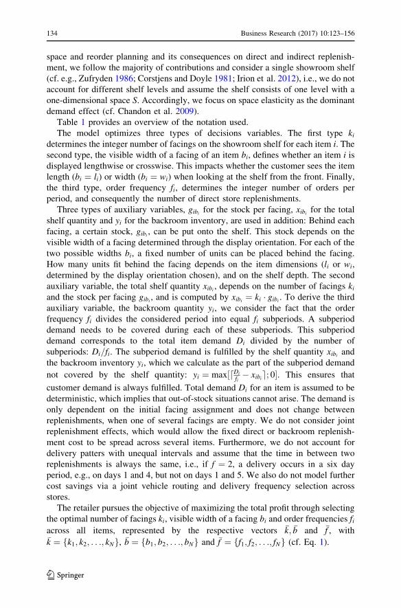
Table 1 provides an overview of the notation used.

The model optimizes three types of decisions variables. The first type kidetermines the integer number of facings on the showroom shelf for each item i. The

second type, the visible width of a facing of an item bi, defines whether an item i is

displayed lengthwise or crosswise. This impacts whether the customer sees the item

length (bi ¼ li) or width (bi ¼ wi) when looking at the shelf from the front. Finally,

the third type, order frequency fi, determines the integer number of orders per

period, and consequently the number of direct store replenishments.

Three types of auxiliary variables, gibi for the stock per facing, xibi for the total

shelf quantity and yi for the backroom inventory, are used in addition: Behind each

facing, a certain stock, gibi , can be put onto the shelf. This stock depends on the

visible width of a facing determined through the display orientation. For each of the

two possible widths bi, a fixed number of units can be placed behind the facing.

How many units fit behind the facing depends on the item dimensions (li or wi,

determined by the display orientation chosen), and on the shelf depth. The second

auxiliary variable, the total shelf quantity xibi , depends on the number of facings kiand the stock per facing gibi , and is computed by xibi ¼ ki � gibi . To derive the third

auxiliary variable, the backroom quantity yi, we consider the fact that the order

frequency fi divides the considered period into equal fi subperiods. A subperiod

demand needs to be covered during each of these subperiods. This subperiod

demand corresponds to the total item demand Di divided by the number of

subperiods: Di=fi. The subperiod demand is fulfilled by the shelf quantity xibi and

the backroom inventory yi, which we calculate as the part of the subperiod demand

not covered by the shelf quantity: yi ¼ max½dDi

fi� xibie; 0�. This ensures that

customer demand is always fulfilled. Total demand Di for an item is assumed to be

deterministic, which implies that out-of-stock situations cannot arise. The demand is

only dependent on the initial facing assignment and does not change between

replenishments, when one of several facings are empty. We do not consider joint

replenishment effects, which would allow the fixed direct or backroom replenish-

ment cost to be spread across several items. Furthermore, we do not account for

delivery patters with unequal intervals and assume that the time in between two

replenishments is always the same, i.e., if f ¼ 2, a delivery occurs in a six day

period, e.g., on days 1 and 4, but not on days 1 and 5. We also do not model further

cost savings via a joint vehicle routing and delivery frequency selection across

stores.

The retailer pursues the objective of maximizing the total profit through selecting

the optimal number of facings ki, visible width of a facing bi and order frequencies fiacross all items, represented by the respective vectors �k; �b and �f , with�k ¼ fk1; k2; . . .; kNg, �b ¼ fb1; b2; . . .; bNg and �f ¼ ff1; f2; . . .; fNg (cf. Eq. 1).


123

maxPð�k; �b; �f Þ ¼X

i2Npiðki; bi; fiÞ ð1Þ

To obtain the item profit pi, we deduct the total cost of direct replenishment CDIRi

and the total cost of backroom replenishment CBRi (cf. Eq. 2) from the total gross

margin of an item. The gross margin of an item is calculated as the product of its

Table 1 Notation

Sets and indices

i Item index

N Set of items a retailer must assign to the shelf, N ¼ f1; 2; . . .; i; . . .;NgKi Set of facings a retailer can select for item i, Ki 2 ½kmin

i ; kmaxi �

Fi Set of order frequencies a retailer can select for item i, Fi 2 ½fmini ; fmax

i �O Set of display orientations a retailer can select from O 2 f1; 2gParameters

B Available backroom space (measured in number of space units, e.g., m2)

ci Unit purchasing costs of item i

CDIRi ;CBR

iTotal direct (DIR) and backroom (BR) replenishment cost of item i

di Minimum demand rate of item i (if it is assigned one facing only and has visible

width of 1)

Di Total demand rate of item i (including space-elasticity effects)

fmini ; fmax

iLower and upper bound on the order frequency of item i

FCDIRi ; FCBR

iFixed costs per replenishment of item i for direct replenishment (DIR) and replenishment

from backroom (BR)

hSRi , hBRi Inventory holding costs per unit of item i in the showroom (SR) and in the backroom

(BR)

kmini ; kmax

iLower and upper bound on the number of facings of item i

li Length of item i (relevant if item i is displayed lengthwise)

mi Gross margin per unit of item i

ri Sales price per unit of item i

S Available showroom shelf space (one-dimensional, front row)

VCDIRi ;VCBR

iVariable costs per replenishment of one unit of item i for direct replenishment (DIR) and

replenishment from backroom (BR)

wi Width of item i (relevant if item i is displayed crosswise)

bi Space-elasticity factor of item i

Decision variables

ki Integer variable; number of facings assigned to item i on the showroom shelf; i 2 N

bi Visible width of a facing of item i depending on its display orienation, i.e., lengthwise

(bi=li) or crosswise (bi=wi), i 2 N

fi Integer variable; order frequency for item i, i.e., the number of times per period an item is

ordered and directly replenished, i 2 N

Auxiliary variables

gibi Number of units of item i per facing (i.e., stock per facing of item i), depending on bi

xibi Integer variable; total shelf quantity for each item i on the showroom shelf with

xibi ¼ ki � gibiyi Integer variable; backroom inventory for each item i with yi ¼ max½dDi

fi� xibie; 0�


123

total demand Di and its unit margin mi. The item unit margin mi corresponds to the

difference between its sales price ri and its purchase cost ci.

piðki; bi; fiÞ ¼ Diðki; biÞ � mi � CDIRi ðki; bi; fiÞ � CBR

i ðki; bi; fiÞ ð2Þ

The total period demand Diðki; biÞ of an item i is a composite function of the

minimum demand di and the facing- and display orientation-dependent demand.

The minimum demand rate di represents the retailer’s forecast for an item that is

independent of the facing and visible facing width (cf. Hansen and Heinsbroek

1979; Hubner and Kuhn 2012; Bianchi-Aguiar et al. 2015a). The forecast may be

based on historical sales, but may also incorporate further demand effects such as

shelf location in the store or other marketing effects. The higher the visibility of an

item, the higher is its demand. The visibility increases with the number of facings ki.

Furthermore, it increases when the item dimension visible to the customer increases,

which is either the item width or the item length. In accordance with prior research

(cf. e.g., Hansen and Heinsbroek 1979; Irion et al. 2012), the facing- and display

orientation-dependent demand rate is a polynomial function of the number of fac-

ings ki allocated to an item, the visible facing width bi and the space-elasticity bi(with 0� bi� 1). Most existing models assume that items have a fixed item width,

as they can be displayed in one display orientation only. We use the demand model

assumed by Irion et al. (2012) to factor in the visible facing width bi. Eq. 3 sum-

marizes the demand calculation applied.

Diðki; biÞ ¼ di � ðki � biÞbi ð3Þ

Total direct replenishment cost (CDIRi ) comprises three parts, as shown in Eq. (4):

fixed replenishment costs for each replenishment of an item (FCDIRi ), variable

replenishment costs for each unit replenished of an item (VCDIRi ) and showroom

inventory holding costs (hSRi ) per unit. Assuming continuous demand, the average

showroom inventory used for calculating the related inventory costs is calculated as

xii=2.

CDIRi ðki; fi; bijxibi¼ki�gibi Þ ¼ FCDIR

i � fi þ VCDIRi � xibi � fi þ hSRi �

xibi2

h ið4Þ

The total backroom replenishment costs (CBRi ) consist of the same three elements

(cf. Eq. 5), where we also need to consider the number of shelf refills from the

backroom (d yixibie) during a subperiod for the fixed replenishment costs, the backroom

inventory yi instead of the showroom shelf quantity, and the backroom’s inventory

holdings costs per unit (hBRi ).

CBRi ki; fi; bijxibi¼ki�gibi� �

¼ FCBRi �

yi

xibi

� �� fi þ VCBR

i � yi � fi þ hBRi �yi

2

� �ð5Þ

Solution approach Equations (3)–(5) contain several non-linear components relating

to the decision variables (e.g., space-elastic demand with ðki � biÞbi or the division of

two variables in the backroom replenishment costs d yixibie). Therefore, it is a non-

linear model. To handle the non-linearity, we precalculate the associated profit


123

piðki; bi; fiÞ and space requirements in the show- and backroom (sSRi ðki; bi; fiÞ,sBRi ðki; bi; fiÞ) for each item i and each possible combination of facings, visible

facing width and order frequencies. The precalculated data is then used in a MIP to

ultimately choose the optimal combination, and thus globally optimize profits. The

usage of a MIP comes with various computational conveniences. We handle the

non-linear model terms outside the optimization model using precalculation.

Suboptimal heuristics are therefore not required. The MIP can be solved optimally

in a time-efficient manner (see runtime tests in Sect. 5.2.1). Finally, the MIP offers

the possibility of adding further model constraints in case these are required from a

practical perspective. An example of this is the restriction that a certain item must

be positioned with a predefined display orientation. This precalculation approach

can be applied because in practice, all decision variables have upper limits. First, a

retailer will only assign a certain number of facings to an item with ki 2 Ki, typi-

cally not more than 20–25 facings. Second, only two values are possible for the

visible width of a facing of item i, i.e., bi ¼ li for lengthwise and bi ¼ wi for

crosswise display orientation. In the MIP model, we decode the visible width of a

facing of item i by o, where o ¼ 1 if bi ¼ li, and by o ¼ 2 if bi ¼ wi. Third, the

frequency of direct replenishments (i.e., orders) cannot exceed the maximum

number of warehouse deliveries with fi 2 Fi, e.g., not more than six times per week.

This allows us to precalculate the profit (denoted as pikof in the MIP) for every item

i and every possible combination of the three decision variables for the predefined

ranges ki 2 Ki, o 2 O and fi 2 Fi, i 2 N. This means that pikof is the profit for item i

if it gets k facings, is given the display orientation o and is ordered f times a period.

Similarly, we precalculate how much showroom (backroom) space item i consumes

for every combination of k, o and f. The respective space consumption is denoted as

sSRikof for the showroom and sBRikof for the backroom.

Using the precalculated profits as data input, the MIP model then selects the

binary variable cikof to indicate how many facings item i should be given, how it is

displayed and how often it should be ordered. The objective function and the

constraints for the resulting model CSRPBS can be formulated as follows:

Max!Pð�cÞ ¼X

i2N

X

k2Ki

X

o2O

X

f2Fipikof � cikof ð6Þ

Subject to:X

i2N

X

k2Ki

X

o2O

X

f2FisSRikof � cikof � S ð7Þ

X

i2N

X

k2Ki

X

o2O

X

f2FisBRikof � cikof �B ð8Þ

X

k2Ki

X

o2O

X

f2Ficikof ¼ 1 8i 2 N ð9Þ

cikof 2 ½0; 1� 8i 2 N; k 2 Ki; o 2 O; f 2 Fi ð10Þ

Equation (6) is the objective function and is the summation of all item-specific

profits. Equations (7) and (8) ensure that showroom shelf S and backroom space


123

B restrictions are met. Finally, Eq. (9) ensures that each item i gets exactly one

combination of facings, item display orientations, and order frequencies. Equa-

tion (10) declares cikof as a binary variable. Note that the available showroom space

S is the one-dimensional shelf length (front row) available for the placement of

facings, e.g., measured in centimeters or meters. In contrast, the size of the back-

room B is measured in space units, e.g., in m2, because in the backroom, items can

theoretically be stored behind each other, whereas items need to be placed next to

each other on showroom shelves for reasons of visibility. Analoguously to that, sSRikofis a one-dimensional length and sBRikof is a two-dimensional area.

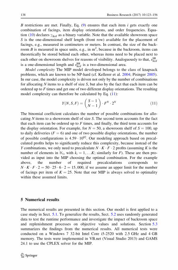
Model complexity The MIP model developed belongs to the class of knapsack

problems, which are known to be NP-hard (cf. Kellerer et al. 2004; Pisinger 2005).

In our case, the model complexity is driven not only by the number of combinations

for allocating N items to a shelf of size S, but also by the fact that each item can be

ordered up to F times and get one of two different display orientations. The resulting

model complexity can therefore be calculated by Eq. (11):

YðN; S;FÞ ¼ S� 1

N � 1

� � FN � 2N ð11Þ

The binomial coefficient calculates the number of possible combinations for allo-

cating N items to a showroom shelf of size S. The second term accounts for the fact

that each item can be ordered up to F times, and finally, the third term accounts for

the display orientation. For example, for N ¼ 50, a showroom shelf of S ¼ 100, up

to daily deliveries (F ¼ 6) and one of two possible display orientations, the number

of possible configurations is 4:59 � 1082. Our modeling approach based on precal-

culated profits helps to significantly reduce this complexity, because instead of the

Y combinations, we only need to precalculate N � K � F � 2 profits (assuming K is the

number of elements in Ki, with ki ¼ 1; . . .K; similarly for F). These are then pro-

vided as input into the MIP choosing the optimal combination. For the example

above, the number of required precalculations corresponds to

N � K � F � 2 ¼ 50 � 25 � 6 � 2 ¼ 15; 000, if we assume an upper limit for the number

of facings per item of K ¼ 25. Note that our MIP is always solved to optimality

within these assumed limits.

5 Numerical results

The numerical results are presented in this section. Our model is first applied to a

case study in Sect. 5.1. To generalize the results, Sect. 5.2 uses randomly generated

data to test the runtime performance and investigate the impact of backroom space

and replenishment processes on objective values and solutions. Section 5.3

summarizes the findings from the numerical results. All numerical tests were

conducted on a Windows 7 32-bit Intel Core i5-2520 with 2.5 GHz and 4 GB

memory. The tests were implemented in VB.net (Visual Studio 2013) and GAMS

24.1 to use the CPLEX solver for the MIP.


123

5.1 Application to real data: case study

This section applies our model to the canned foods assortment of a German grocery

retailer.

Data applied We consider the product category for which we also obtained the

process descriptions and cost structures from our time and motion study. This

category encompasses 70 different items. In this category, the retailer only puts the

items onto the shelf in case packs (i.e., cartons) and not in single customer units

(i.e., cans). We treat one carton as one facing and each carton contains a quantity of

six or twelve units. The display orientation-dependent stock per facing gibi is

derived here as follows: As the shelf depth does not allow case packs to be put

behind each other regardless of a crosswise or lengthwise positioning, the stock per

facing is given by the quantity per carton. Please note that here the space-elasticity

effect is reflected in Eq. (3) by the b-value for the crosswise/lengthwise display

orientation of the facing, i.e., demand increases when the larger of the two carton

dimensions is displayed.

We consider a sales period of one week. The average minimum demand di of the

items i 2 N is between 1 and 110 units per week. For determining di, we first

measured the average total demand Di across 10 months with the current number of

facings ki, the current visible width of a facing bi, an assumed space elasticity of biand then recalculated the average minimum demand di using Eq. (3). We assume

that space elasticity is equal for all items within the canned foods category. The

items are sold for a price of 0.50 € � ri� 2.49 €. For reasons of confidentiality, thecorresponding values for unit, replenishment and inventory cost cannot be provided.

Showroom shelf space is limited to S ¼ 5920 cm and backroom utilization is

currently very low, which is why we can consider backroom space capacity to be

unlimited. At the time of data collection, the retailer assigned between 1 and 21

facings to the items, which all have a lengthwise display orientation. The number of

facings was determined according to a sales-proportional allocation (SPA) rule,

which assigns shelf space to items based on their share of category sales, but ignores

replenishment cost (cf. Hubner and Kuhn 2012). The item length li is 14.8 cm

� li� 40.0 cm and item width wi is 22.4 cm �wi� 41.7 cm. All items are

currently ordered twice a week (fi ¼ 2).

Approaches analyzed To show the extent to which the retailer benefits from the

model, we investigate the following modeling approaches: [1] ‘‘Status quo’’—which

represents the number of facings and display orientation as observed in the current

shelf-space assignment and a given order frequency of f ¼ 2 for all items. To ensure

comparability, we evaluate the observed values of all decision variables using the

objective function (cf. Eq. 6) of the CSRPBS-model. To compute margins and

replenishment costs ‘‘a posteriori’’, we apply the respective ‘‘a posteriori’’ model,

denoted as CSRP*. Furthermore, we ensure that all constraints (7–10) are fulfilled.

From here, we derive the profit potential in steps: Approaches [2] and [3] are partial

optimizations, where either order frequencies (approach [2], model CSRPBS*ð�f Þ) orfacings and display orientations (approach [3], model CSRPBS*ð�k; �bÞ) are

optimized. In [2] we keep k and b as per current and in [3] we do so for f. All


123

profit components are evaluated by applying the respective ‘‘a posteriori’’

calculation for the non-optimized variables. Finally, in approach [4] ‘‘Integrated

optimization’’, the CSRPBSð�k; �b; �f Þ model optimizes k, b and f simultaneously, and

therefore, shows the full potential. This model corresponds to the CSRPBS

introduced in Sect. 4. To highlight the differences to approaches [1]–[3], we add

here the superscript for the decision variables. Table 2 summarizes the respective

assumptions for each modeling approach:

Results Figure 3 illustrates the advantage of the fully integrated model

(CSRPBSð�k; �b; �f Þ) over the partial optimization models and the status quo for

different values of the space elasticity. The analysis reveals several insights: First,

independent of space elasticity, a significant opportunity exists for the retailer to

improve the status quo. If we assume a space elasticity of 15% (cf. Eisend 2014 who

identified an average of 17%), the full potential of integrated optimization compared

to the status quo (approach [4] vs. [1]) amounts to approximately 29%. Second, the

retailer also profits from partial optimization, i.e., only optimizing order frequencies

([2] vs. [1]) or facings and display orientations ([3] vs. [1]). The higher potential

clearly lies in the optimization of facings and display orientations. However, the

results from [4] show that an integrated perspective is still better than partial

optimization. Finally, we see that the advantage of the integrated model

(CSRPBSð�k; �b; �f Þ) over pure shelf-space optimization (CSRPBS*ð�k; �bÞ) diminishes

with increasing space elasticity. This is due to the fact that the importance of

assigning the right amount of space to high-margin items increases as space

elasticity and the connected demand increase, which is achieved by both models.

Simultaneously, the magnitude of replenishment cost decreases and so does the

advantage of the fully integrated over the shelf-space optimization model.

To better understand the latter, Fig. 4 shows the absolute values for total profits

(P

i2N pi), total gross margins (P

i2N Di � mi) and total replenishment cost

(P

i2N CDIRi and

Pi2N CBR

i ) for the four approaches. The profit increase is mainly

driven by the increase in gross margins, while replenishment costs are much lower

in magnitude. With increasing space elasticity, the impact of the gross margin effect

rises even higher. Note that in CSRP* and CSRPBS*ð�f Þ, ki and bi are determined

regardless of the space elasticity, and are therefore, identical across all b-values.However, the gross margin increases also for these two approaches, because the

Table 2 Different approaches for case study

Approach [1] Status quo Partial optimization Full optimization

[2] Order

frequency

[3] Facings/Displ.

orient.

[4] Integrated

Model

applied

CSRP* CSRPBS*ð�f Þ CSRPBS*ð�k; �bÞ CSRPBSð�k; �b; �f Þ

Optimization None Order frequency f Facings k Facings k

Variables (all as per

current)

Visible facing width b Visible facing width

b

Order frequency f


123

demand realized increases with an increase in the assumed space elasticity (see

Eq. 2).

Table 3 shows the changes in solution structure, i.e., facings, visible facing width

and order frequencies. The comparison of the partial and full optimization models

25

20%

35

45

10

030%

5

5%

50

30

20

40

15

25%10%0% 15%

Space elasticityPercent

Profit advantagePercent

CSRPfBS* advantage over CSRP*

CSRPk,bBS* advantage over CSRP*

CSRPk,b,fBS advantage over CSRP*

Fig. 3 Relative profit advantage of integrated and partial optimization models over status quo

20%

2,250

1,750

1,2501,000

500250

30%

1,500

2,000

750

25%10%5% 15%0%

Total gross marginEUR


2,000

1,2501,000

20%5%0%0

30%15% 25%10%

1,7501,500

750500250

Total profitEUR


30%15% 20% 25%5% 10%0%

5

10

0

30

25

20

15


Total backroom replenishment costEUR

40

120140

1008060

5% 20% 30%15% 25%

20

10%0%0

Total direct replenishment costEUR


CSRPk,bBS*CSRPf

BS* CSRPk,b,fBSCSRP*

Fig. 4 Total profits, total gross margins and total replenishment cost for each modeling approach


123

with the status quo shows significant differences in all three optimization variables,

e.g., 90% of all items get a different number of facings in the full optimization

compared to the status quo. Furthermore, the comparison of the full optimization to

the partial optimizations shows that there is still a significant share of items with

differences in either order frequencies (21.4% with different order frequencies, [2]

vs. [4]) or facings and display orientations (15.7% with different facings, 2.9% with

different display orientation, [3] vs. [4]).

5.2 Generalization using randomly generated data

After having shown how the retailer can use our model to increase profits, we can

now generalize these insights by conducting more extensive analyses with randomly

generated data. Section 5.2.1 describes the data used and the test setting.

Section 5.2.2 then provides runtime tests. Section 5.2.3 investigates the impact of

backroom availability on profits and solution structures and Sect. 5.2.4 analyzes the

profit advantages retailers can achieve when thoroughly accounting for replenish-

ment processes. We compare our model to a sales-proportional allocation rule in

Sect. 5.2.5 and develop an extension to account for assortment decisions in

Sect. 5.2.6.

5.2.1 Data applied, models and test bed

The data generation process is based on the data obtained from the case study. If not

stated otherwise, we use a uniform distribution to randomly generate the item-

specific parameters which are within the following intervals: di 2 ½50; 70�;ri 2 ½10; 20�; ci 2 ½75% � ri; 80% � ri�; gibi 2 ½3; 5�; VCDIR

i ¼ ½0:02; 0:06�;VCBR

i ¼ ½0:06; 0:10�; FCDIRi ¼ ½0:08; 0:12�; FCBR

i ¼ ½0:16; 0:24�; hSRi 2 ½2:5% �ri; 3:5% � ri� and hBRi 2 ½1:5% � ci; 2:0% � ci�. In other words, replenishment from

the backroom is twice as expensive as direct replenishment on average, and

inventory holding costs are lower in the showroom than in the backroom. Space

elasticity of the single items bi is assumed to vary between 0 and 35%. To focus on

the core effects, we assume wi ¼ li ¼ 1, if not stated otherwise. Furthermore, we set

Table 3 Changes in solution structure

Models Approaches Change of

k b f

CSRP* versus CSRPBS*ð�f Þ [1] versus [2] – – 95.7%

CSRP* versus CSRPBS*ð�k; �bÞ [1] versus [3] 88.6% 61.4% –

CSRP* versus CSRPBSð�k; �b; �f Þ [1] versus [4] 90.0% 58.6% 88.6%

CSRPBS*ð�f Þ versus CSRPBS*ð�k; �bÞ [2] versus [3] 88.6% 61.4% 95.7%

CSRPBS*ð�f Þ versus CSRPBSð�k; �b; �f Þ [2] versus [4] 90.0% 57.1% 21.4%

CSRPBS*ð�k; �bÞ versus CSRPBSð�k; �b; �f Þ [3] versus [4] 15.7% 2.9% 88.6%

Scenario with bi ¼ 15%


123

K ¼ 15 and F ¼ 6 for the precalculations, were K(F) corresponds to the number of

elements in Ki with ki ¼ 1; . . .;K (Fi with fi ¼ 1; . . .;F).We use the model CSRPBS to optimize facings, visible facing width and order

frequencies, and solve it using the MIP introduced in Sect. 4 (cf. Eqs. 6–10). The

CSRP* model is used to evaluate the impact of ignoring specific effects (e.g.,

replenishment cost) ‘‘a posteriori’’. The measured effects are averages across 100

randomly generated instances of N items.

5.2.2 Runtime test

Table 4 shows the average runtime for different problem instances and shows that

our model can efficiently generate optimal results even for large-scale problem

instances. While we assumed wi ¼ li ¼ 1 for all instances up to N ¼ 400 items, for

the instance with N ¼ 2000, S ¼ 60; 000 and B ¼ 30; 000 we randomly generated

item dimensions with wi 2 ½2; 10� and li 2 ½5; 15� to test runtime performance under

more complex assumptions. The model still generates optimal results in a minimum

amount of time in less than a minute runtime on average.

The CSRPBS is a knapsack problem. It becomes a hard knapsack problem when

item weight (in our case the shelf space occupied by the item) and the item

contribution (in our case the unit margin) are strongly correlated (cf. Pisinger 2005).

To test the performance of our approach on hard knapsack problems, we run a

further test on instances with N ¼ 2000, S ¼ 60; 000 and B ¼ 30; 000, where unit

margins and space occupied correlate with R2 ¼ 0:9. The average runtime for these

100 instances is 78.06 s, with a minimum of 62.34 s and a maximum of 93.47 s,

which shows that our approach can also handle hard knapsack problems efficiently.

5.2.3 Impact of backroom space on profits and solution structures

To investigate the impact of backroom availability on profits and solutions

structures, we first present a 2-item example below and then extend the analysis to a

more comprehensive set of randomly generated data.

2-item example We consider two items (1 and 2) with identical demand and cost

parameters. Both items have a length of li ¼ 1 and a width of wi ¼ 2. The stock per

facing gibi depends on the visible facing width and is 1 in case of a lengthwise

orientation, and 2 in case of a crosswise orientation. The only difference between

the two items is that item 1 has a high space elasticity and item 2 has none

(b1 ¼ 30%; b2 ¼ 0%). Below, we analyze how facings, display orientations, order

Table 4 Runtime tests for different problem sizes, in seconds

Number of items N 5 50 100 200 400 2000

Showroom space S 20 200 400 800 1000 60,000

Backroom space B 5 100 200 400 500 30,000

Ø Runtime 0.86 1.48 1.91 3.21 6.62 45.93

Average of 100 examples


123

frequencies and backroom quantities change if showroom and backroom space

increase.

Figure 5 shows that with a showroom space of S ¼ 6 and no backroom space

(B ¼ 0), the highly space-elastic item 1 receives k1 ¼ 5 facings and is replenished

f1 ¼ 2 times a week. Item 2 receives only the minimum of k2 ¼ 1 facing because its

space elasticity is zero. Item 2 needs to be ordered more often (at f2 ¼ 6) to still

satisfy the demand for it. Both items are displayed lengthwise, and therefore, have a

stock per facing of only one unit. If backroom space now becomes available (while

showroom space remains the same), it is beneficial to decrease order frequencies for

item 2 from f2 ¼ 6 (B� 1) to f2 ¼ 2 (B� 4) and instead replenish it indirectly from

the backroom where inventory holding cost is lower (y2 ¼ 2). If showroom space

S is doubled from six to twelve (and no backroom exists), item 1 now receives only

k1 ¼ 3 facings, which are displayed crosswise. Item 2 is also positioned crosswise

and receives k2 ¼ 1 facings. Both items receive a stock of two units per facing due

to the crosswise orientations. Two interesting observations are to be made: First, a

showroom shelf space of only eight out of a total of twelve is occupied. The reason

why the shelf space is not fully occupied is the following: Further space could

theoretically be assigned to the highly space-elastic item 1, but since this would

induce additional space-elastic demand that cannot fully be supplied by the

showroom inventory, backroom quantities would need to be kept for item 1 to

satisfy the demand for it (compare scenario with S ¼ 12 and B ¼ 4, where y1 ¼ 2).

Since no backroom exists, item 1 remains at three facings. Second, the crosswise

S B Optimal shelf configuration (showroom shelf) f* y*

Item 1Space

1 2High space elasticity item No space elasticity item

6 0/1 1 1 1 1 1 2

1 1 1 1 1 22/3

1 1 1 1 1 24-6

a1

a1

a1

a2

12 0/1

a1

a1

a1 22/3

a1

a1

a14/5 a

1a

1a

2

a1

a1

a16/7 a

1a

1 2

a1

a1

a18-11 a

1a

1 2

a1

a1

a112 a

1a

1a

2

f* y*

Item 2Showroomusage

Backroomusage

6 0 2 0 6 0

6 2 2 0 3 1

6 4 2 0 2 2

8 0 2 0 3 0

7 2 2 0 3 1

12 4 1 2 3 0

11 6 1 2 3 1

11 8 1 2 2 2

12 12 1 2 1 4

Profit

100.0%

105.2%

106.7%

102.2%

105.6%

116.6%

120.0%

121.5%

122.0%

Fig. 5 Analysis of availability of showroom and backroom space on profit and solution structure, 2-itemexample (changes of decision variables between subsequent scenarios are in bold)


123

display orientation of item 2 allows for a stock of 2 units to be placed on the shelf.

This allows for a decrease in the order frequency from f2 ¼ 6 (at S ¼ 6;B ¼ 0) to

f2 ¼ 3 (at S ¼ 12;B ¼ 0). Because b2 ¼ 0% and due to showroom inventory

holding cost, it is also not beneficial to use the remaining shelf space for further

units of item 2.

Obviously, a backroom space of B ¼ 2 (or 3) is not yet sufficient to further

decrease f2, but it can be used to reduce the inventory held in the showroom. The

display orientation of item 2 therefore changes back to lengthwise, which results in

a stock of only one. Inventory moves to the backroom, where it is cheaper to keep

stock (y2 ¼ 1). If backroom space increases to B ¼ 4 (or 5), priority is immediately

given to item 1, since now the additional space-elastic demand caused by an

increased number of facings (k1 ¼ 5) can be served from the backroom, which is

completely occupied with item 1 (y1 ¼ 2). This requires putting item 2 back in a

crosswise orientation, since this allows a shelf quantity of two units that could not

be kept in the backroom fully occupied by item 1 (y2 ¼ 0). At B ¼ 6 (or 7), item 2’s

display orientation can again be changed to lengthwise, which shifts inventory

holding cost from the expensive showroom to the less expensive backroom (y2 ¼ 1).

At B ¼ 8 (or 9,10,11), the additional backroom space is used to lower f2 to f2 ¼ 2

again, similarly to the three scenarios with S ¼ 6. Finally, at B ¼ 12, f2 can even

decrease to f2 ¼ 1. Obviously backroom space is not enough to keep the lengthwise

orientation. Item 2 is placed crosswise, and a stock of g2 ¼ 2 units must be kept on

the showroom shelf.

The example shows that items with a high space elasticity should clearly be given

priority in shelf-space assignment. Furthermore, the trade-offs between availability

of showroom and backroom space, facings, order frequencies and display

orientations are illustrated. Even with this stylized example, it generally becomes

evident that the availability of backroom space impacts optimal facings, display

orientations and order frequencies. We can conclude, if retailers have the

opportunity to use backrooms for intermediate storage, they should leverage them,

because backroom space allows for more flexibility in planning showroom shelf-

space and in-store replenishment processes.

Extended analysis To underline the impact of backroom space B on profit and

solution structures, and to generalize the findings above, we analyzed additional

randomly generated data sets. Each set contains N ¼ 50 items. To focus on the main

effects, we ignore the display orientation and set li ¼ wi ¼ 1. We set F ¼ 6 and

K ¼ 15 and assume a showroom shelf space of S ¼ 200 and in the basic scenario a

backroom space of B ¼ 100, which is varied below. For each analysis, we report the

average of 100 randomly generated data sets.

Figure 6 shows the impact of changing backroom size on financial performance

(i.e., total profits, total gross margins, total direct and backroom replenishment cost).

As seen above in the 2-item example, an increase in backroom space results in

increased total profits. This is due to an increase in demand as well as lower total

direct replenishment costs, i.e., direct replenishment and showroom inventory

holding cost. By providing more flexibility in the form of additional backroom

space B, more space for beneficial items can be reserved on the showroom shelf

space to generate more sales (resulting in higher total gross margins) and the


123

backroom can be more extensively used to refill showroom shelves if this is cost-

beneficial. On the other hand, this induces an increase in total backroom

replenishment costs, i.e., backroom replenishment and backroom inventory holding

cost, which is shown in the right-hand graph.

Figure 7 provides the changes in the solution structure: Up to 80% of the items

are given a different number of facings k if backroom space B decreases. An

increase in backroom space B analogously induces changes in shelf-space

assignment, but the upper limit of K ¼ 15 limits the magnitude of this effect: Up

to 20% of the items are given a different number of facings k if backroom space B is

doubled.

In terms of order frequencies f, similar observations apply. Up to 54% of the

items have a change in order frequencies f if backroom space B changes. The right-

hand graph shows that the average number of orders per week decreases, as more

backroom space B becomes available. A larger backroom space B allows for

decreased order frequencies f, because backroom space can be used to store items

and then replenish shelves from there. Note that as soon as backroom space

B becomes available, order frequencies f increase slightly at first before gradually

decreasing. This is because less profitable and less space-elastic items can be moved

-3

-2

-1

0

1

-100% -50% 0% 50% 100%

Change in total profitPercent

Change in backroom spacePercent

-4

-3

-2

-1

0

1

-100% -50% 0% 50% 100%


Change in total gross marginPercent

-1.5-1.0-0.5

00.5

1.01.52.02.53.0

-100% -50% 0% 50% 100%

Change in total direct replenishment costPercent


-100

-80

-60

-40

-20

0

20

-100% -50% 0% 50% 100%

Change in total backroom replenishment costPercent

Change in backroom space

Percent

Fig. 6 Impact of backroom availability on financial performance


123

to the backroom to free up additional space in the showroom. This space is used to

allocate more facings to high-profit and high space-elasticity items, which generates

additional demand. Because showroom shelf S is scarce, this demand increase

enforces an increase in order frequencies. These effects decrease in magnitude the

more backroom space B becomes available, because it can be used to fulfill the

additional demand without further increases in order frequencies f.

5.2.4 Impact of replenishment and inventory costs on profit and solution structure

To analyze the impact of replenishment and inventory costs, we conducted an ‘‘a

posteriori’’ analysis. We considered a retailer who neglects the relevant cost

elements and just accounts for item demand and margins, i.e.,

VCDIRi ¼ VCBR

i ¼ FCDIRi ¼ FCBR

i ¼ hSRi ¼ hBRi ¼ 0. Based on these assumptions,

we ran the CSRP*-model and ‘‘a posteriori’’ evaluated the solution structure (k,

b and f) assuming the actual costs. We set S ¼ 800 and vary the available backroom

space from B 2 ½0� 100�. Item dimensions vary as follows: wi 2 ½2; 10� and

li 2 ½5; 15�. For these different backroom sizes, Table 5 presents the advantage a

retailer has when correctly accounting for relevant cost elements and considering

facings, display orientation and order frequency optimization from an integrated

0

10

20

30

40

50

60

70

80

-100% -50% 0% 50% 100%

Share of items with changes in showroom facingsPercent


0

10

20

30

40

50

60

-100% -50% 0% 50% 100%

Share of items with changes in order frequenciesPercent


5.0

5.1

5.2

5.3

5.4

5.5

5.6

5.7

-100% -50% 0% 50% 100%

Ø number of orders/week


Note: Figures show average of 100 randomly generated data sets

Fig. 7 Impact of backroom availability on solution structure

Table 5 Impact of neglecting replenishment and inventory costs on profits and solution structure for

varying backroom sizes

Total profit increase [%] 13.8–21.5

Share of items with changes in facings k [%] 68.1–69.1

Share of items with changes in visible facing width b [%] 42.9–45.2

Share of items with changes in order frequency f [%] 77.3–87.1

Backroom usage [%]

‘‘A posteriori’’ (CSRP*) 79.8–85.3

Optimal (CSRPBS) 45.0–63.3

S ¼ 800, B 2 ½0� 100�, 100 randomly generated data sets evaluated for each scenario


123

perspective. Depending on the size of the available backroom, the profit is up to

around 22% higher and solution structures change significantly: 70% of the items

are given a different number of facings k, 77–87% a different order frequency f and

43–45% a different visible facing width b. Moreover, we see that backroom

utilization is much higher if not all relevant costs are properly accounted for:

Backroom utilization is 80–85% versus 45–63% if replenishment and inventory

holding costs are properly incorporated.

5.2.5 Comparison to sales-proportional allocation rule

This section compares the results of the CSRPBS to those generated with a sales-

proportional allocation rule (SPA). For the SPA, we again use an ‘‘a posteriori’’

evaluation. This benchmark is denoted as CSRP* like in Sect. 5.1. The SPA rule

does not define the display orientation. To allow a good comparison we assume that

li ¼ wi and no display orientation is required. We use the same N ¼ 50 item data

sets as before. In the SPA, the overall showroom space S is allocated to the items in

proportion to their sales share, and order frequencies are fixed for all items. We

analyze six scenarios, with fi ¼ 1; . . .; 6. Table 6 shows the profit advantage of the

optimization model (that optimizes for fi and ki); the magnitude increases as order

frequencies rise. Furthermore, we see the significant differences in solution

structures. Note that the profit potential here is lower than in the case study

(Sect. 5.1) because the unit margins we assumed here are lower than the unit

margins in the case.

5.2.6 Impact of assortment decisions

In this section, we show how assortment decisions can be incorporated into the

CSRPBS. The resulting model is denoted as CASRPBS, whereas the additional ‘‘A’’

represents the assortment decision. So far, we have assumed that the assortment is

determined in a previous planning step and that the retailer must assign all items of

set N to the shelf, i.e., we did not allow zero facings ki ¼ 0. Including the

assortment decision allows more flexibility for two reasons: (1) Solutions for

situations with S\N, can now be generated and items delisted. (2) Even if S�N, it

might be beneficial to delist specific items and use the shelf space for more

beneficial items, e.g., items with a higher margin and/or space elasticity. The

inclusion of assortment decisions requires an adaptation of the demand function (cf.

Eq. 3) to account for additional demand arousing from out-of-assortment (OOA)

Table 6 Profit advantage of CSRPBS over CSRP* and changes in solution structure

Order frequency [times per week] 1 2 3 4 5 6

Profit advantage of CSRPBS over CSRP* [%] 5.33 5.33 6.91 8.58 10.30 12.07

Share of items w/facing changes [%] �� 98.00 ��!

Share of items w/order frequency changes [%] 58.00 62.00 92.00 94.00 98.00 98.00

S ¼ 1000, B ¼ 100, 100 randomly generated data sets evaluated for each scenario


123

situations (Smith and Agrawal 2000; Kok and Fisher 2007). OOA substitution

expresses the customer’s willingness to buy an alternative item if the preferred item

is not listed. By taking substitution into account, demand and the profit for an item

i also depend on the availability of all other items j; j 6¼ i. This extension increases

the combinatorial complexity of our model, since the cross-product interdependen-

cies result in a quadratic problem and the isolated precalculation of the item-specific

profits as input to the MIP (see Sect. 4) does not capture these product interlinks

anymore.

The model complexity Y of the CSRPBS with YðN; S;FÞ ¼ S� 1

N � 1

� � FN � 2N

increases to YðN; S;FÞ ¼ N þ S� 1

S

� � FN � 2N for the CASRPBS when includ-

ing the assortment decision. Due to the increased complexity and product interlinks,

we need a heuristic to iteratively determine the total demand Di for an item

considering the availability of other items. We therefore first develop the extended

solution approach for the CASRPBS and then complete numerical examples to

show its efficiency and the impact of assortment decisions.

Extension of model and solution approach To incorporate assortment decisions,

we differentiate the total set of items N into the set of listed items Nþ and the set of

delisted items N�, with Nþ;N� � N, Nþ [N� ¼ N and Nþ \N� ¼ ø. Equa-

tion (3) is extended in the following way to account for OOA substitution:

Dið�k; biÞ ¼ di � ðki � biÞbi þ dOOAi ð�kÞ ð12Þ

Total demand Di for item i now not only consists of its own space-elastic demand

(di � ðki � biÞbi ) but also of the OOA demand caused by the delisting of other items

(dOOAi ð�kÞ). We calculate this new demand component as follows:

dOOAi ð�kÞ ¼X

j2N�dj � cji 8i 2 Nþ ð13Þ

Equation (13) shows that if an item j is delisted (j 2 N� and therefore, kj ¼ 0) a

certain share (cji) of its minimum demand (dj) is substituted by item i. cji is the

substitution rate between items j and i. We allow one round of substitution as in

Smith and Agrawal (2000), Kok and Fisher (2007) or Hubner et al. (2016), i.e., sales

are lost if the substitute is not available either. In the following, we use the

aggregated substitution rate di for an item, which corresponds to the likelihood that

a delisted item gets substituted at all, and then assume that this aggregated rate is

split equally among the remaining items, i.e., cji ¼ diNþ�1, 8j 6¼ i (cf. Kok et al.

2015). To account for assortment decisions and to thoroughly compute the asso-

ciated demand function, we apply the following heuristic:

• Step 1 Ignore OOA substitution by setting dOOAi ð�kÞ ¼ 0 in Eq. (12) and solve the

MIP as introduced in Eqs. (6) to (10), including ki ¼ 0 in Ki, 8i 2 N

• Step 2 Update the demand for all items using Eqs. (12) and (13) with the values

for ki and bi obtained in Step 1


123

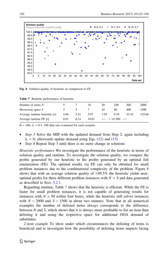
• Step 3 Solve the MIP with the updated demand from Step 2, again including

ki ¼ 0; afterwards update demand using Eqs. (12) and (13)

• Step 4 Repeat Step 3 until there is no more change in solutions

Heuristic performance We investigate the performance of the heuristic in terms of

solution quality and runtime. To investigate the solution quality, we compare the

profits generated by our heuristic to the profits generated by an optimal full

enumeration (FE). The optimal results via FE can only be obtained for small

problem instances due to the combinatorial complexity of the problem. Figure 8

shows that with an average solution quality of[99.5% the heuristic yields near-

optimal profits for three different problem instances with N[ S and data generated

as described in Sect. 5.2.1.

Regarding runtime, Table 7 shows that the heuristic is efficient. While the FE is

faster for small problem instances, it is not capable of generating results for

instances with N[ 50 within four hours, while the heuristic still solves instances

with N ¼ 2000 and S ¼ 1500 in about two minutes. Note that in all numerical

examples the number of delisted items always corresponds to the difference

between N and S, which shows that it is always more profitable to list an item than

delisting it and using the respective space for additional OOA demand of

substitutes.

2-item example To show under which circumstances the delisting of items is

beneficial and to investigate how the possibility of delisting items impacts facing

50

96.0

53520

98.5

95.5

99.5

45 85

94.5

6555 95

96.5

97.5

7520 70

97.0

99.0

90

98.0

5 15 100

100.0

601094.0

4030

95.0

80

Solution qualityPercent (heuristic profit/FE profit)

Data set

N 10, S 7N 5, S 3 N 7, S 5

Fig. 8 Solution quality of heuristic in comparison to FE

Table 7 Runtime performance of heuristic

Number of items N 5 7 10 50 100 500 2000

Showroom space S 3 5 7 45 80 400 1500

Average runtime heuristic [s] 4.66 5.41 5.97 7.54 9.45 43.19 125.66

Average runtime FE [s] 0.01 0.14 10.01 � [ 14; 400 �!

B ¼ 100, di ¼ 0:3, 100 data sets evaluated for each scenario


123

and order decisions, we again use the 2-item example. Items 1 and 2 compete for a

showroom space of S ¼ 2, i.e., the retailer can split this space or allocate it

exclusively to either one of the items. In the base scenario [1], both items are

completely identical and we choose item parameters as in the 2-item example in

Sect. 5.2.3.

To focus on the core effects, we again assume li ¼ wi ¼ 1, i 2 f1; 2g. From here,

we investigate the extended problem if item 1 is highly space-elastic and item 2 is

not (Scenario [2]), if item 1 has a high and item 2 a low margin ((ri � ciÞ=ci,Scenario [3]), and if replenishment cost factors Costi, i.e., VC

DIRi , VCBR

i , FCDIRi and

FCBRi of item 2 are 2–100 times as high as for item 1 (Scenarios [4a–4d]).

Table 8 shows that the showroom space is allocated equally (k1 ¼ k2 ¼ 1) if both

items are identical (Sc. [1]). This only changes across the seven scenarios if either

margins are extremely different ([3]), where then only the high-margin item is listed

(k1 ¼ 2 and k2 ¼ 0), or if replenishment costs are very (unrealistically) different

(Sc. [4d]), where item 2 with the 100 times higher replenishment costs is again

delisted. Significant differences in space elasticities do not result in the delisting of

items (Sc. [2]). In summary, if space is sufficient to potentially list all items,

assortment decisions are only likely to be impacted by the joint shelf-space and

reorder planning if items significantly differ in their margin. The results from this

2-item example are intuitive, and the findings do apply to larger instances in the

same way.

5.3 Summary of numerical results

The application of our model to real and randomly generated data sets reveal several

important insights. First, we show in a case study that a retailer can increase profits

by around 29% compared to the status quo if our model is applied in full.

Simultaneously optimizing facings, display orientations and order frequencies is

superior to the strictly shelf-space-based optimization of facings and display

orientation, without optimizing order frequencies. This underlines the importance of

an integrated perspective on shelf-space optimization and in-store replenishment

Table 8 Assortment changes depending on margin, space elasticity and cost

Scenario Description Facings Order frequency

k1 k2 f1 f2

[1] Both items equal 1 1 2 2

[2] b1 ¼ 35%; b2 ¼ 0% 1 1 2 2

[3] Margin1 = 50%, Margin2 = 5% 2 0 2 0

[4a] Cost2 = 2 � Cost1 1 1 2 2

[4b] Cost2 = 5 � Cost1 1 1 2 2

[4c] Cost2 = 10 � Cost1 1 1 2 2

[4d] Cost2 = 100 � Cost1 2 0 2 0

S ¼ 2, B ¼ 10


123

processes. Second, our model can be efficiently solved by a MIP model. The results

consistently are optimal and even generated within a minimum amount of time for

large-scale instances. Third, if backroom space is available, retailers can make use

of it by assigning more showroom space to highly profitable items and moving less

profitable items to the backroom, from where they are replenished more frequently.

In other words, the available backroom space gives more degrees of freedom to the

retailer in terms of shelf-space optimization. Fourth, our model can be extended to

account for assortment decisions, which is especially relevant for situations where

the available shelf space is not sufficient to list all possible items of a category.

Finally, the profit advantage a retailer has when taking an integrated approach to

facing, display orientation and order frequency optimization can amount up to

around 22% compared to a case where facings and display orientation are optimized

without considering the related costs for in-store replenishment. This is because

significantly different solution structures result in terms of facings, display

orientation and order frequencies if replenishment processes are neglected.

6 Conclusion and outlook

In this paper, we presented a capacitated shelf-space optimization model that

contributes to the existing literature by accounting for in-store replenishment and

the availability of backroom space. The model maximizes retail profits while

considering costs for direct and backroom replenishment, cost for inventory, limited

showroom and backroom space as well as space-elastic demand. Retailers are

provided with additional flexibility from the optimized display orientations of items.

We have quantified the relevant in-store processes cost by means of a time and

motion study for a German retailer. Our process descriptions serve to further define

in greater detail the in-store processes and cost types identified in the existing

literature. To solve the resulting non-linear problem, we developed a mixed-integer

model. Even for large-scale problems, our model yields optimal results efficiently

within a feasible amount of time. We applied our model to the retailer’s canned

foods category and showed how profits can be increased significantly by applying

our model. After the results were presented to the retailer, he decided to change his

current approach to shelf-space and in-store replenishment planning by applying our

model. Furthermore, we have shown that an integrated perspective on shelf-space

and replenishment optimization is crucial for retailers, because backroom space and

replenishment cost have a significant impact on retail profits and shelf-space

planning. An integrated perspective for shelf planning is specifically important,

since in practice shelf-space decisions are made by a central sales planning unit

which oftentimes ignores the consequences of shelf planning on in-store operations.

Our model will help retailers to develop this integrated perspective.

Limitations and future areas of research The limitations of our model point to a

variety of future areas of research. We follow the general literature on shelf-space

management and assume a deterministic and stationary demand for the tactical

problem. Because of this, demand is always satisfied. Hence, one area is to further

generalize the demand modeling. Some authors argue that demand volatility can be


123

handled with exogenously determined safety stocks. The resulting shelf space for

the safety stock needs to be deducted from the total shelf space and only the

remaining space can be distributed. However, our modeling approach has the

advantage of being flexible enough to determine safety stocks endogenously. As

safety stocks protect against uncertainty in demand (demand volatility) and supply

(lead time volatility), the impact of both decision variables (i.e., the impact of the

number of facings on the demand and the impact of the order frequency on supply)

need to be taken into account. Hence, for all precalculated combinations of the

decisions variables, one can calculate the safety stocks accordingly within the

model. Furthermore, our model and solution approach is a good starting point to

account for further demand effects. Focusing on demand volatility would imply the

development of a stochastic model for our decision problem with replenishment

costs to account for demand variations (cf. e.g., Hubner and Schaal 2016a). In such

cases, out-of-stock substitutions resulting from potentially insufficient shelf and

backroom quantities for specific items would need to be taken into consideration as

well (cf. e.g., Kok and Fisher 2007; Hubner et al. 2016). A stochastic model would

need to balance the trade-offs between understock and overstock situations, which is

specifically relevant in the case of perishable items. These additional costs can be

included in the precalculations. Apart from stochastic demand, further demand

effects, such as item positioning (cf. e.g., Lim et al. 2004; Bianchi-Aguiar et al.

2015b) or cross-space elasticities (cf. e.g., Corstjens and Doyle 1981), would be

worth considering when the model is applied to certain categories with these

demand effects.

Our model concentrates on the cost associated with direct and indirect

replenishment of shelves. Future models could incorporate further decisions and

associated cost, such as upstream supply chain decisions and the cost of deliveries

from warehouses to stores (cf. Sternbeck and Kuhn 2014; Holzapfel et al. 2016).

Moreover, retail managers typically try to keep shelves as filled as possible, since

empty space is generally believed to have a negative impact on sales (cf. Baron

et al. 2011). This may result in differentiated refill costs. We have shown that our

solution approach is capable of solving a problem with up to 2000 items within less

than a minute. Although shelf-space and reordering decisions are typically made for

each category separately, our model could be extended for store-wide shelf-space

optimization across all categories, where common order patterns for different

categories would also be considered.

Finally, the investigation of multi-store environments can be considered. A

corresponding model would support retailers in deciding whether planograms

should be more standardized or adjusted to store-specific needs. Such a model

would need to balance the trade-off between store-specific demand fulfillment and

the efficiency of upstream logistics processes.

Our optimization model takes the perspective of a retailer who wants to optimize

category profit. In contrast, a manufacturer follows the objective of brand profit

optimization, which raises the topic of ‘‘category captainship’’ (cf e.g., Kurtulus and

Toktay 2011; Martınez-de Albeniz and Roels 2011). A comprehensive study will

need to address all the relevant subjects of negotiation between manufacturers and

retailers, such as assortment, prices and shelf space.


123

The model and solution approach proposed within this paper will be a good

starting point to address the open areas of research mentioned above.

Open Access This article is distributed under the terms of the Creative Commons Attribution 4.0

International License (http://creativecommons.org/licenses/by/4.0/), which permits unrestricted use, dis-

tribution, and reproduction in any medium, provided you give appropriate credit to the original

author(s) and the source, provide a link to the Creative Commons license, and indicate if changes were

made.

References

Barnes, R.M. 1949. Motion and time study. New York: Wiley.

Baron, O., O. Berman, and D. Perry. 2011. Shelf space management when demand depends on the

inventory level. Production and Operations Management 20 (5): 714–726.

Bianchi-Aguiar, T., M.A. Carravilla, and J.F. Oliveira. 2015a. Replicating shelf space allocation solutions

across retail stores. Working paper University Porto.

Bianchi-Aguiar, T., A. Hubner, M.A. Carravilla, and J.F. Oliveira. 2016. Retail shelf space planning

problems: A comprehensive review and classification framework. Working paper University Porto.

Bianchi-Aguiar, T., E. Silva, L. Guimaraes, M.A. Carravilla, and J.F. Oliveira. 2015b. Allocating

products on shelves under merchandising rules: Multi-level product families with display directions.

Working paper University Porto.

Borin, N., P. Farris, and J. Freeland. 1994. A model for determining retail product category assortment

and shelf space allocation. Decision Sciences 25 (3): 359–384.

Broekmeulen, R., K. van Donselaar, J. Fransoo, and T. van Woensel. 2006. The opportunity of excess

shelf space in grocery retail store. Operations Research 49: 710–719.

Chandon, P., W.J. Hutchinson, E.T. Bradlow, and S.H. Young. 2009. Does in-store marketing work?

Effects of the number and position of shelf facings on brand attention and evaluation at the point of

purchase. Journal of Marketing 73 (November): 1–17.

Corstjens, M., and P. Doyle. 1981. A model for optimizing retail space allocations. Management Science

27 (7): 822–833.

Cox, K. 1964. The responsiveness of food sales to shelf space changes in supermarkets. Journal of

Marketing Research 1 (2): 63–67.

Curseu, A., T. van Woensel, J. Fransoo, K. van Donselaar, and R. Broekmeulen. 2009. Modelling

handling operations in grocery retail stores: An empirical analysis. Journal of the Operational

Research Society 60 (2): 200–214.

Curhan, R.C. 1972. The relationship between shelf space and unit sales in supermarkets. Journal of

Marketing Research 9 (4): 406–412.

DeHoratius, N., and T. Zeynep. 2015. The role of execution in managing product availability. In Retail

supply chain management. International series in operations research & management science, vol.

122, ed. N. Agrawal, and S.A. Smith, 53–77. New York: Springer.

Desmet, P., and V. Renaudin. 1998. Estimation of product category sales responsiveness to allocated shelf

space. International Journal of Research in Marketing 15 (5): 443–457.

Donselaar, KHv, V. Gaur, Tv Woensel, R.A. Broekmeulen, and J.C. Fransoo. 2010. Ordering behavior in

retail stores and implications for automated replenishment. Management Science 56 (5): 766–784.

Dreze, X., S.J. Hoch, and M.E. Purk. 1994. Shelf management and space elasticity. Journal of Retailing

70 (4): 301–326.

EHI Retail Institute. 2014. Retail data 2014: Structure, key figures and profiles of international retailing.

Eisend, M. 2014. Shelf space elasticity: A meta-analysis. Journal of Retailing 90: 168–181.

Eroglu, C., B.D. Williams, and M.A. Waller. 2013. The backroom effect in retail operations. Production

and Operations Management 22 (4): 915–923.

Fisher, M. 2009. Or forum-rocket science retailing: The 2006 Philip Mccord Morse Lecture. Operations

Research 57 (3): 527–540.

Frank, R.E., and W.F. Massy. 1970. Shelf position and space effects on sales. Journal of Marketing

Research 7 (1): 59–66.

Geismar, H.N., M. Dawande, B.P. Murthi, and C. Sriskandarajah. 2015. Maximizing revenue through

two-dimensional shelf-space allocation. Production and Operations Management 24: 1148–1163.


123

http://creativecommons.org/licenses/by/4.0/

Gutgeld, Y., S. Sauer, and T. Wachinger. 2009. Growth-but how? Akzente 3 (3): 14–19.

Hansen, J.M., S. Raut, and S. Swami. 2010. Retail shelf allocation: A comparative analysis of heuristic

and meta-heuristic approaches. Journal of Retailing 86 (1): 94–105.

Hansen, P., and H. Heinsbroek. 1979. Product selection and space allocation in supermarkets. European

Journal of Operational Research 3 (6): 474–484.

Hariga, M.A., and A. Al-Ahmari. 2013. An integrated retail space allocation and lot sizing models under

vendor managed inventory and consignment stock arrangements. Computers and Industrial

Engineering 64 (1): 45–55.

Hariga, M.A., A. Al-Ahmari, and A.-R.A. Mohamed. 2007. A joint optimisation model for inventory

replenishment, product assortment, shelf space and display area allocation decisions. European

Journal of Operational Research 181 (1): 239–251.

Holzapfel, A., A. Hubner, H. Kuhn, and M.G. Sternbeck. 2016. Delivery pattern and transportation

planning in grocery retailing. European Journal of Operational Research 252 (1): 54–68.

Hubner, A.H., and H. Kuhn. 2011. Shelf and inventory management with space-elastic demand. In

Operations research proceedings 2010, ed. B. Hu, K. Morasch, M. Siegle, and S. Pickl, 405–410.

Berlin: Springer.

Hubner, A.H., and H. Kuhn. 2012. Retail category management: A state-of-the-art review of quantitative

research and software applications in assortment and shelf space management. Omega 40 (2):

199–209.

Hubner, A., and K. Schaal. 2016. When does cross-space elasticity matter in shelf-space planning? A

decision analytics approach. Working Paper KU Eichstatt-Ingolstadt.

Hubner, A., and K. Schaal. 2017. A shelf-space optimization model when demand is stochastic and space-

elastic. Omega 68: 139–154.

Hubner, A.H., H. Kuhn, and M.G. Sternbeck. 2013. Demand and supply chain planning in grocery retail:

An operations planning framework. International Journal of Retail & Distribution Management 41

(7): 512–530.

Hubner, A., H. Kuhn, and S. Kuhn. 2016. An efficient algorithm for capacitated assortment planning with

stochastic demand and substitution. European Journal of Operational Research 250 (2): 505–520.

Hwang, H., B. Choi, and G. Lee. 2009. A genetic algorithm approach to an integrated problem of shelf

space design and item allocation. Computers and Industrial Engineering 56 (3): 809–820.

Hwang, H., B. Choi, and M.-J. Lee. 2005. A model for shelf space allocation and inventory control

considering location and inventory level effects on demand. International Journal of Production

Economics 97 (2): 185–195.

Irion, J., J.-C. Lu, F. Al-Khayyal, and Y.-C. Tsao. 2012. A piecewise linearization framework for retail

shelf space management models. European Journal of Operational Research 222 (1): 122–136.

Kellerer, H., U. Pferschy, and D. Pisinger. 2004. Knapsack problems. Berlin: Springer.

Kok, G., M.L. Fisher, and R. Vaidyanathan. 2015. Assortment planning: Review of literature and industry

practice. In Retail supply chain management. International series in operations research &

management science, vol. 223, ed. N. Agrawal, and S.A. Smith, 175–236. New York: Springer.

Kok, G.A., and M.L. Fisher. 2007. Demand estimation and assortment optimization under substitution:

Methodology and application. Operations Research 55 (6): 1001–1021.

Kotzab, H., G. Reiner, and C. Teller. 2007. Beschreibung, Analyse und Bewertung von Instore-

Logistikprozessen. Zeitschrift fur Betriebswirtschaft 77 (11): 1135–1158.

Kotzab, H., S. Seuring, M. Muller, and G. Reiner (eds.). 2005. Research methodologies in supply chain

management. Heidelberg: Springer.

Kotzab, H., and C. Teller. 2005. Development and empirical test of a grocery retail instore logistics

model. British Food Journal 107 (8): 594–605.

Kuhn, H., and M.G. Sternbeck. 2013. Integrative retail logistics: An exploratory study. Operations

Management Research 6 (1–2): 2–18.

Kurtulus, M., and B.L. Toktay. 2011. Category captainship vs. retailer category management and limited

retail shelf space. Production and Operations Management 20 (1): 47–56.

Lim, A., B. Rodrigues, and X. Zhang. 2004. Metaheuristics with local search techniques for retail shelf-

space optimization. Management Science 50 (1): 117–131.

Martınez-de Albeniz, V., and G. Roels. 2011. Competing for shelf space. Production and Operations

Management 20 (1): 32–46.

Maynard, H.B., G.J. Stegemerten, and J.L. Schwab. 1948. Methods-time measurement. New York:

McGraw-Hill.


123

Murray, C.C., D. Talukdar, and A. Gosavi. 2010. Joint optimization of product price, display orientation

and shelf-space allocation in retail category management: Special issue: Modeling retail

phenomena. Journal of Retailing 86 (2): 125–136.

Niebel, B.W. 1988. Motion and time study. Homewood: Richard D. Irwin.

Pires, M., J. Pratasy, J. Lizy, and P. Amorim. 2016. A framework for designing backroom areas in grocery

stores. International Journal of Retailing and Distritubtion Management (forthcoming)Pisinger, D. 2005. Where are the hard knapsack problems? Computers & Operations Research 32 (9):

2271–2284.

Ramaseshan, B., N.R. Achuthan, and R. Collinson. 2008. Decision support tool for retail shelf space

optimization. International Journal of Information Technology & Decision Making 7 (3): 547–565.

Ramaseshan, B., N.R. Achuthan, and R. Collinson. 2009. A retail category management model

integrating shelf space and inventory levels. Asia-Pacific Journal of Operational Research 26 (4):

457–478.

Reiner, G., C. Teller, and H. Kotzab. 2013. Analyzing the efficient execution on in-store logistics

processes in grocery retailing—The case of dairy products. Production and Operations Management

22 (4): 924–939.

Russell, Ra, and T.L. Urban. 2010. The location and allocation of products and product families on retail

shelves. Annals of Operations Research 179: 131–147.

Seuring, P.D.S., P.D.M. Muller, M. Westhaus, and R. Morana. 2005. Conducting a literature review—The

example of sustainability in supply chains. Research methodologies in supply chain management.

Physica-Verlag: HD, 91–106.

Smith, S.A., and N. Agrawal. 2000. Management of multi-item retail inventory systems with demand

substitution. Operations Research 48 (1): 50–64.

Sternbeck, M.G., and H. Kuhn. 2014. An integrative approach to determine store delivery patterns in

grocery retailing. Transportation Research Part E: Logistics and Transportation Review 70:

205–224.

Urban, T.L. 1998. An inventory-theoretic approach to product assortment and shelf-space allocation.

Journal of Retailing 74 (1): 15–35.

Yang, M.-H., and W.-C. Chen. 1999. A study on shelf space allocation and management. International

Journal of Production Economics 60–61 (4): 309–317.

Zelst, S, K. van Donselaar, T. van Woensel, R. Broekmeulen, and J. Fransoo. 2009. Logistics drivers for

shelf stacking in grocery retail stores: Potential for efficiency improvement. International Journal of

Production Economics 121 (2): 620–632.

Zufryden, F.S. 1986. A dynamic programming approach for product selection and supermarket shelf-

space allocation. Journal of the Operational Research Society 37 (4): 413–422.


123

Documents

Effect of replenishment and backroom on retail shelf-space