EFFECT OF RADIATION MODELS ON COAL …eccc.uno.edu/pdf/Lu-Wang radiation in gasification IMECE2012-86997.pdf · entrained flow gasifier developed for an IGCC process under ... Aspen

1 Copyright © 2012 by ASME

Proceedings of the ASME 2012 International Mechanical Engineering Congress & Exposition IMECE2012

November 9-15, 2012, Houston, Texas, USA

IMECE2012-86997

EFFECT OF RADIATION MODELS ON COAL GASIFICATION SIMULATION

Xijia Lu and Ting Wang Energy Conversion & Conservation Center

University of New Orleans New Orleans, LA 70148-222

504-280-2389, [email protected] and 504-280-7183, [email protected]

ABSTRACT Adequate modeling of radiation heat transfer is important in CFD simulation of coal gasification process. In an entrained-flow gasifer, the non-participating effect of coal particles, soot, ashes, and reactive gases could significantly affect the temperature distribution in the gasifier and hence affects the local reaction rate and life expectancy of wall materials. For slagging type gasifiers, radiation further affects the forming process of corrosive slag on the wall which can expedite degradation of the refractory lining in the gasifier. For these reasons, this paper focuses on investigating applications of five different radiation models to coal gasification process, including Discrete Transfer Radiation Model (DTRM), P-1 Radiation Model, Rosseland Radiation Model, Surface-to-Surface (S2S) Radiation Model, and Discrete Ordinates (DO) Radiation Model. The objective is to identify the pros and cons of each model's applicability to the gasification process and determine which radiation model is most appropriate for simulating the process in entrained-flow gasifiers.

The Eulerian-Lagrangian approach is applied to solve the Navier-Stokes equations, nine species transport equations, and seven global reactions consisting of three heterogeneous reactions and four homogeneous reactions. The coal particles are tracked with the Lagrangian method. Six cases are studied—one without the radiation model and the other five with different radiation models. The result reveals that the various radiation models yield uncomfortably large uncertainties in predicting syngas composition, syngas temperature, and wall temperature. The Rosseland model does not yield reasonable and realistic results for gasification process. The DTRM model predicts very high syngas and wall temperatures in the dry coal feed case. In the one-stage coal slurry case, DTRM result is close to the S2S result. The P1 method seems to behave stably and is robust in predicting the syngas temperature and composition; it yields the result most close to the mean, but it seems to underpredict the gasifier’s inner wall temperature. INTRODUCTION Gasification is an incomplete combustion process, converting a variety of carbon-based feedstock to clean

synthetic gas (syngas), which is primarily a mixture of hydrogen (H2) and carbon-monoxide (CO) as fuels. Feedstock is partially combusted with oxygen at high temperature and pressure with less than 30% of the required oxygen for complete combustion (i.e., the stoichiometric amount) being provided. The syngas produced can be used as a fuel, usually for boilers or gas turbines to generate electricity; it can also be made into a substitute natural gas (SNG) or hydrogen gas and/or other chemical products. Gasification technology is applicable to any type of carbon-based feedstock, such as coal, heavy refinery residues, petroleum coke, biomass, and municipal wastes. To help understand the gasification process in gasifiers and subsequently use the learned knowledge to guide designs of more compact, more cost effective, and higher performance gasifiers, computational fluid dynamics (CFD) has been widely employed as a powerful tool to achieve these goals. In the majority of industrial combustion devices, thermal radiation plays a significant role for an important energy transfer. Even though the coal gasification process undergoes a partial combustion process, thermal radiation may still play a very important role in heat and energy transfer between different gas species, coal particles, as well as the wall of gasifier. Furthermore, in order to extend the lifetime of the refractory bricks and to reduce the maintenance cost, keeping the process temperature relatively low, but still effective in performing the gasification process and cracking the volatiles, is one of the important goals for gasification research. Therefore, an accurate and computationally efficient thermal radiation model is needed to predict flame shape and temperature distributions of syngas at the wall of gasifier. In this study, five radiation models are applied into gasification simulation: Discrete Transfer Radiation Model (DTRM), P-1 Radiation Model, Rosseland Radiation Model, Surface-to-Surface (S2S) Radiation Model, and Discrete Ordinates (DO) Radiation Model. The objectives are to identify the pros and cons of each model's applicability to gasification process and determine which radiation model is most suitable for simulating gasification process in entrained-flow gasifiers with a consideration of the gasifier’s geometry, radiative properties


of participating medium (mainly CO, CO2, H2 and water vapor), and coal particles interactions. 1.1 Literature Review of Radiation Models Implemented in Gasification Simulation Chen et al. developed a three-dimensional simulation model for entrained-flow coal gasifiers, which applied an extended coal-gas mixture fraction model with the Multi Solids Progress Variables (MSPV) method. The model employed four mixture fractions separately track the variable coal off-gases from the coal devolatilization, char-O2, char-CO2, and char-H2O reactions. Chen et al. performed a series of numerical simulations for a 200 ton per day (tpd) two-stage air blown entrained flow gasifier developed for an IGCC process under various operation conditions (heterogeneous reaction rate, coal type, particle size, and air/coal partitioning to the two stages). In these computational models, the discrete transfer method (DTRM) based on the solution of the fundamental radiative transfer equation within discrete solid angles was used [1].

Bockelie et al. developed a comprehensive CFD modeling tool (GLACIER) to simulate entrained-flow gasifiers, including a single-stage, down-fired system and a two-stage system with multiple feed inlets. They used DO radiation model which included the heat transfer for absorbing-emitting, anisotropically scattering, turbulent, and sooting media. The radiative intensity field was solved based on properties of the surfaces and participating media, and the resulting local flux divergence appeared as a source term in the gas phase energy equation [2].

The U.S. Department of Energy/National Energy Technology Laboratory (NETL) developed a 3D CFD model of two commercial-sized coal gasifiers [3]. The commercial CFD software, FLUENT, was used to model the first gasifier, which was a two-stage, entrained-flow, slurry-fed coal gasifier. The Eulerian-Lagrangian method was used in conjunction with the discrete phase model to simulate the entrained-flow gasification process. The second gasifier was a scaled-up design of a transport gasifier. The NETL open source MFIX (Multiphase Flow Interphase Exchanges) Eulerian-Eulerian model was used for this dense multiphase transport gasifier. MFIX is a general-purpose hydrodynamic model that describes chemical reactions and heat transfer in dense or dilute fluid-solids flows, typically occurring in energy conversion and chemical processing reactors. The radiative heat transfer is not considered in this model. NETL has also developed an Advanced Process Engineering Co-Simulator (APECS) that combines CFD models and plant-wide simulation. APECS enables NETL to couple its CFD models with the steady-state process simulator, Aspen Plus.

Chodankar et al. developed a steady state model to estimate the gas production from Underground Coal Gasification (UCG) Process. This model featured surface reactions of coal char with gasification medium to produce combustible gaseous product, and predicts gas composition, temperature and gross calorific value of product gas across the gasification channel. P1 radiation model was used in their study [4]. Ajilkumar performed a numerical simulation on a steam-assisted tubular coal gasification process. The syngas temperature, carbon conversion, heating value of the exit gas, and cold gas efficiency were predicted and compared with the

experimental data. P1 model was chosen as the radiation model in their simulation model study [5]. Wu et al. used 3D CFD model for the simulation of an entrained coal slurry gasification process. The effect of particle size on coal conversion, as well as the effect of the coal slurry concentration and molar ratio of oxygen/carbon on the gasifier performance, was investigated. The P1 radiation model was also used in their study [6]. Chen used a 3-D simulation model to investigate the effect of oxygen/carbon ratio and water/coal ratio on the entrained flow coal gasification process.. P1 model was selected as the radiation model in his study [7]. From 2005 to 2011, Silaen and Wang have conducted a series of study of entrained-flow gasification process using the commercial CFD solver, FLUENT. In these studies, they investigated the effects of several parameters on gasification performance, including the coal input condition (slurry or dry powder), oxidant (oxygen-blown or air-blown), wall cooling, flow injection angles, and various coal distributions between the two stages [8] [9] [10]. They also investigated the effects of various turbulence models and devolatilization models on the result of gasification simulations [11]. Furthermore, they compared the effect of instantaneous, equilibrium and finite rate gasification models on the entrained flow coal gasification process [12]. Lu and Wang investigated the effect of Water-Gas-Shift (WGS) reaction rate on gasification process. They found that most of the published WGS reaction rates, both under catalytic and non-catalytic conditions, are too fast in gasification simulation process. By adjusting the pre-exponential rate constant value (A) against experimental data, calibrated WGS reaction rate were obtained [13]. In all of the above studies, only the P1 radiation model was used.

In collaboration with the research team of Industrial Technology Research Institute (ITRI), Wang and Silaen effectively employed the CFD gasification model to investigate gasification process under the influences of different part loads, two different injectors, and three different slagging tap sizes [14] [15] [16]. In 2011, Wang, et al. performed the simulation on the effects of potential fuel injection techniques on gasification performance in order to help design the top-loaded fuel injection arrangement for an entrained-flow gasifier using a coal-water slurry as the input feedstock. Two specific arrangements were investigated: (a) coaxial, dual-jet impingement with the coal slurry in the center jet and oxygen in the outer jet and (b) four-jet impingement with two single coal-slurry jets and two single oxygen jets [17]. Wang and Lu investigated the performance of a syngas quench cooling design in the ITRI downdraft entrained flow gasifier. Numerical simulation was performed to investigate the effect of different injection stage of cooling water, and water gap level on syngas composition, higher heating value and temperature at exit of gasifier [18]. Again, only the P1 radiation model was used. Based on the above literature review, only the P1 model has been widely used in gasification simulation. Although Chen et al. [1] and Bockelie et al. [2] used DTRM and DO radiation models respectively, to the authors’ knowledge, no study has been published in the public domain to compare the results obtained from different radiation models. The lack of information on the uncertainty of simulated results resulting


from employment of different radiation models has motivated the investigation conducted in this study. 1.2 Review of Radiation Models

1.2.1 Radiation of Participating Media (Gas Phase)

In coal gasification process, CO, H2, CO2, and water vapor are produced and participate in radiant heat transfer by the virtue of interaction of infrared radiation with vibrational and rotational modes of energy absorption by gaseous molecules.

Two aspects of radiation heat transfer in participating media need to be modeled: one is the radiant energy transfer in the participating media, described by the radiative transfer equation, the other is the absorption, emission, and scattering of radiation by the participating media itself.

For the first aspect, the transfer equation alone with a number of representative rays could be solved by discrete transfer method described by Lockwood and Shah [19] as well as by the discrete ordinate method described by Chandrasekhar [20]. The accuracy of the solution is the function of numerical errors that could be reduced to any required level by solving enough number of rays or directions.

For the second aspect, several models for participating media have been introduced in conjunction with the flow field by simultaneously solving the fluid flow equations such as the mixed grey gas models introduced by Hottel and Sarofim [21]. Grosshandler introduced the total transmittance non-homogeneous model, which is a simplified model, using total transmittance data to predict the radiance emanating from non-isothermal, variable concentration carbon dioxide and water-vapor mixtures. Computational times using this model are two-orders of magnitude less than that required by the Goody statistical narrow-band model with Curtis-Godson approximation, but with a sacrifice in accuracy of less than 10% [22].

Edwards and Balakrishnan introduced exponential wide band model and presented the generalized expressions for the calculation of the emissivity, absorptivity, and other relevant radiation properties of molecular gases [23]. Cumber et al. adapted a spectral version of the exponential-wide band for implementation within a computational fluid dynamic framework. They also showed that the spectral wide band approach is in a reasonable agreement with experimental data and achieves accuracy comparable to that of the narrow band model in total quantities while requiring almost one order of magnitude less of computational time [24]. 1.2.2 Radiation of Combustion Particles (Solid Phase) During the coal gasification process, radiation of solid particles also plays an important role in heat transfer since the coal particles will go through preheating, devolatilization, ignition, and partial combustion process at the beginning stage of the gasification process. For the field of radiation heat transfer of solid particles, most of the studies have been carried out in coal combustion system. Sarofim and Hottel gave a detailed review of the importance of radiative heat transfer in combustion systems [25]. All combustion processes are very complicated. There are intermediate chemical reactions in sequence or parallel, intermittent generation of a variety of

intermediate species, generation of soot, agglomeration of soot particles, and partial burning of the soot sequentially. Since thermal radiation contributes greatly to the heat and energy transfer mechanism of combustion, fundamental understanding and appropriate modeling of the processes of radiation of combustion particles need to be addressed and implemented for gasification process, which involves partial combustion and several other reactions. 1.2.2.1 Coal Particles and Fly Ash Dispersions To calculate the radiative properties of arbitrary size distributions of coal particles, their complex index of refraction as a function of wavelength and temperature must be investigated. Foster and Howarth have employed a Fresnel reflectance technique to measure the complex refractive index of coals at different ranks [26]. Brewster and Kunitomo questioned the validity of the reflectance technique applied to the coal. They measured the absorption index of some Australian coals to be less than 0.05 in the infrared by using a transmission technique for small coal particles [27].

Viskanta et al. summarized the representative values for the complex index of refraction in the near infrared for different coals and ashes, such as carbon, anthracite, bituminous, lignite, and fly ash. They also found that variations with particle distribution functions are relatively minor, and the different index of refraction made a difference only for mid-sized particles [28]. Buckius and Hwang analyzed the extinction and absorption coefficients, as well as the asymmetry factor for polydispersions of absorbing spherical particles. By showing that dimensionless spectral radiation properties are independent of the explicit size distribution of the particle, they indicated the usefulness of the dimensionless and mean properties for defining the optical properties of coal particles which are wavelength dependent [29]. 1.2.2.2 Char In the radiation heat transfer process of coal gasification, optical constants of char are considered to be more important than that of coal since the coal devolatilization time is generally insignificant compared with the char burning and char gasification time. Grosshandler and Monteiro investigated the absorption and scattering of thermal radiation within a dilute cloud of pulverized coal and char. They proposed an empirical equation of the form αλ = 0.78 + 0.18/λ1/2 for all coals and chars within 5 percent in the spectral region of λ= 1.2–5.3 µm. They also recommended a single total hemispherical absorptivity of 0.89 for heat transfer calculation in pulverized coal and char clouds, if the particles can be assumed to act as Mie scatters and if the volume fraction of ash and soot particles is small [30]. Brewster and Kunitomo determined the extinction efficiency from transmissivity measurements on micron-sized char suspensions by a particle extinction technique using compressed KBr tablets [31]. IM and Ahluwalia conducted a dispersion analysis of the transmissivity measurement by Brewster and Kunitomo on char particles dispersed in infrared transmissive KBr pellets. They introduced some question as to the uniqueness of the optical constants inferred purely from the extinction measurement. In order to properly resolve the contributions of absorption and scattering to extinction efficiency, they


recognized that it is necessary to measure a second independent variable [32]. 1.2.2.3 Soot Soot particles are produced in fuel-rich flames, or fuel-rich parts of flames, as a result of incomplete combustion of hydrocarbon fuels. In coal gasification process, soot production coincides with the stage of volatile matters being driven from the coal. Since soot particles are very small and are generally at the same temperature as the flame, they strongly emit thermal radiation in a continuous spectrum over the infrared region. Experiments have shown that soot emission often is considerably stronger than combustion gases’

emission. Foster and Howarth were first to report experimental measurements for the complex index of refraction of hydrocarbon soot based on various carbon black powders [33]. Lee and Tien used the dispersion theory applied to a two bound and one free-electron oscillator model to analyze the optical constants of soot. Their results show that the infrared optical properties of soot are relatively independent of the ratio of fuel hydrogen to carbon and the molecular structure of soot. Thus their dispersion constants can be treated as some mean values applicable to many fuels [34]. Since the soot effect on gasification process is very complicated, it is not investigated in the current study.

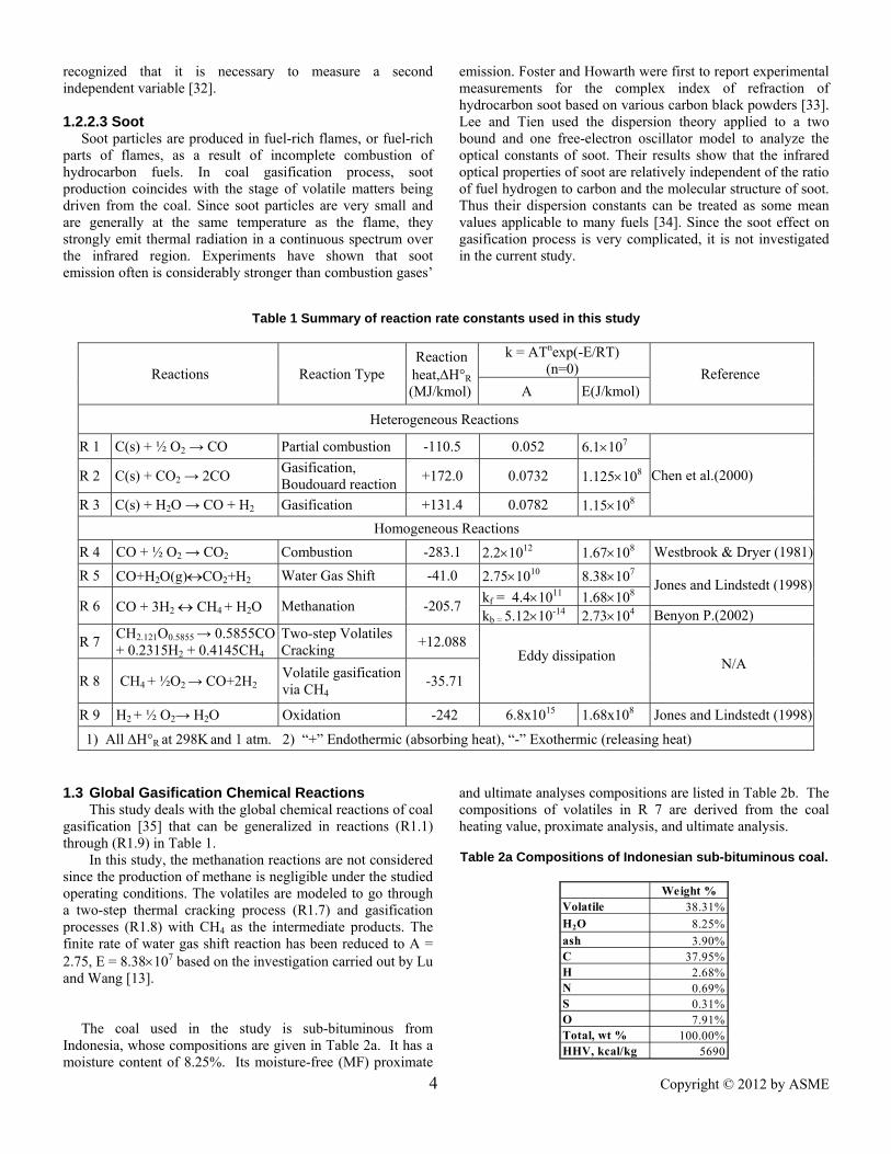
Table 1 Summary of reaction rate constants used in this study

1.3 Global Gasification Chemical Reactions This study deals with the global chemical reactions of coal gasification [35] that can be generalized in reactions (R1.1) through (R1.9) in Table 1.

In this study, the methanation reactions are not considered since the production of methane is negligible under the studied operating conditions. The volatiles are modeled to go through a two-step thermal cracking process (R1.7) and gasification processes (R1.8) with CH4 as the intermediate products. The finite rate of water gas shift reaction has been reduced to A = 2.75, E = 8.38×107 based on the investigation carried out by Lu and Wang [13]. The coal used in the study is sub-bituminous from Indonesia, whose compositions are given in Table 2a. It has a moisture content of 8.25%. Its moisture-free (MF) proximate

and ultimate analyses compositions are listed in Table 2b. The compositions of volatiles in R 7 are derived from the coal heating value, proximate analysis, and ultimate analysis.

Table 2a Compositions of Indonesian sub-bituminous coal.

Weight %Volatile 38.31%H2O 8.25%ash 3.90%C 37.95%H 2.68%N 0.69%S 0.31%O 7.91%Total, wt % 100.00%HHV, kcal/kg 5690

Reactions Reaction Type Reaction

heat,ΔH°R (MJ/kmol)

k = ATnexp(-E/RT) (n=0) Reference

A E(J/kmol)

Heterogeneous Reactions

R 1 C(s) + ½ O2 → CO Partial combustion -110.5 0.052 6.1×107

Chen et al.(2000) R 2 C(s) + CO2 → 2CO Gasification, Boudouard reaction +172.0 0.0732 1.125×108

R 3 C(s) + H2O → CO + H2 Gasification +131.4 0.0782 1.15×108 Homogeneous Reactions

R 4 CO + ½ O2 → CO2 Combustion -283.1 2.2×1012 1.67×108 Westbrook & Dryer (1981)R 5 CO+H2O(g)↔CO2+H2 Water Gas Shift -41.0 2.75×1010 8.38×107 Jones and Lindstedt (1998)R 6 CO + 3H2 ↔ CH4 + H2O Methanation -205.7 kf = 4.4×1011 1.68×108

kb = 5.12×10-14 2.73×104 Benyon P.(2002)

R 7 CH2.121O0.5855 → 0.5855CO + 0.2315H2 + 0.4145CH4

Two-step Volatiles Cracking +12.088

Eddy dissipation N/A

R 8 CH4 + ½O2 → CO+2H2 Volatile gasification via CH4

-35.71

R 9 H2 + ½ O2→ H2O Oxidation -242 6.8x1015 1.68x108 Jones and Lindstedt (1998)

1) All ΔH°R at 298K and 1 atm. 2) “+” Endothermic (absorbing heat), “-” Exothermic (releasing heat)


Table 2b Moisture-free (MF) compositions of Indonesian sub-bituminous coal. Proximate Analysis (MF), wt% Ultimate Analysis (MF), wt%Volatile 51.29 C 73.32Fixed Carbon (FC) 47.54 H 4.56Ash 1.17 O 20.12

100.00 N 0.72S 0.11Ash 1.17

100.00

2.0 COMPUTATIONAL MODEL 2.1 Governing Equations The time-averaged, steady-state Navier-Stokes equations, as well as the mass and energy conservation equations, are solved. The governing equations for the conservations of mass, momentum, and energy are given as:

(1)

(2)

(3)

where the symmetric stress tensor, τij, is given by:

. (4)

The equation for species transport is given by:

. (5)

2.2 Turbulence Models The detailed analysis of the effect of various turbulence models on the gasification process has been documented in a previous paper by Silaen and Wang [11]. They compared the results of five turbulence models, including Standard k-ε, RNG (Re-Normalized Group) k-ε, Standard k-ω Model, Shear Stress Transport (SST) k-ω Model, and Reynolds Stress Model (RSM). They reported that the standard RSM model achieved the most consistent results and the k-ε turbulence model was found to yield reasonable results next to the RSM model, but the RSM model used almost seven times more computational time than the k-ε model. Following their conclusions without repeating the same process again, the standard k-ε turbulence model with enhanced wall function is used in this study to reduce the computational time. 2.3 Discrete Phases (Coal Particles or Liquid Droplets) Discrete phases include coal particles and liquid droplets. The Lagrangian method is adopted in this study to track each particle. Particles in the airflow can encounter inertia and hydrodynamic drag. Because of the forces experienced by a

droplet in a flow field, the particles can be either accelerated or decelerated. The velocity change can be formulated by

mpdvp/dt = Fd + Fg + Fo (6)

where Fd is the drag of the fluid on the particle and Fg is the gravity. Fo represents the other body forces, which typically include the “virtual mass” force (such as centrifugal force, coriolis force, magnetic force, etc.), thermophoretic force, Brownian force, Saffman's lift force, etc. Vp is the particle velocity (vector). In this study, Saffman's lift force reaches about 30% of Fg, so it is included in this study. When the coal is injected through the injectors, the water content in the coal is treated as being in the condensed phase (i.e. liquid water), which can't be lumped into the continuous phase, so the liquid water is atomized into small droplets. Theoretically, evaporation occurs at two stages: (a) when the temperature is higher than the saturation temperature (based on the local water vapor concentration,) water evaporates from the droplet’s surface, and the evaporation is controlled by the water vapor partial pressure until 100% relative humidity is achieved; and (b) when the boiling temperature (determined by the gas-water mixture pressure) is reached, water continues to evaporate even though the relative humidity reaches 100%. After the moisture is evaporated due to either high temperature or low moisture partial pressure, the vapor diffuses into the main flow and is transported away. The rate of vaporization is governed by the concentration difference between the surface and the gas stream, and the corresponding mass change rate of the droplet can be given by:

(7)

where kc is the mass transfer coefficient and Cs is the concentration of the vapor at the particle’s surface, which is evaluated by assuming that the flow over the surface is saturated. C∞ is the vapor concentration of the bulk flow, obtained by solving the transport equations. The values of kc can be calculated from empirical correlations by Ranz and Marshall [36],

. (8)

where Sh is the Sherwood number, Sc is the Schmidt number (defined as ν/D), D is the diffusion coefficient of vapor in the bulk flow. Red is the Reynolds number, defined as uν/d, u is the slip velocity between the particle and the gas, and d is the particle diameter. When the particle temperature reaches the boiling point, the following equation can be used to evaluate its evaporation rate:

(9)

where λ is the heat conductivity of the gas/air, and hfg is the droplet latent heat. cp is the specific heat of the bulk flow. The particle temperature can also be changed due to heat transfer between particles and the continuous phase. The particle’s sensible heat changes depending on the convective heat transfer, latent heat (hfg), species reaction heat (Hreac), and radiation, as shown in the following equation:

( ) mjii

Sρux

=∂∂

( ) ( ) jjiijij

jjii

Suuρτxx

Pgρuρux

+′′−∂∂

+∂∂

−=∂∂

( ) hipii

ipi

SμΦTuρcxTλ

xTuρc

x++⎟⎟

⎠

⎞⎜⎜⎝

⎛′′−

∂∂

∂∂

=∂∂

⎟⎟⎠

⎞⎜⎜⎝

⎛

∂∂

−∂∂

+∂

∂=

k

kij

j

i

i

jij x

uδ32

xu

xu

μτ

( ) jjii

ji

iji

i

SCuρxC

ρDx

Cρux

+⎟⎟⎠

⎞⎜⎜⎝

⎛′′−

∂

∂

∂∂

=∂∂

)C(Ckπddt

dmsc

2d∞−=

0.330.5d

cd Sc0.6Re2.0

DdkSh +==

( ) pfgp0.5d

2d c/h/)TT(c1ln)0.46Re(2.0dλπd

dtdm

−++⎟⎠⎞

⎜⎝⎛= ∞


(10) where the convective heat transfer coefficient (h) can be obtained with a similar empirical correlation to Eq. 11:

(11)

where Nu is the Nusselt number, and Pr is the Prandtl number. Eq. (10) is used for both water droplets and coal particles. Stochastic Tracking of Particles -- The various turbulence models are based on the time-averaged equations. Using this flow velocity to trace the droplet will result in an averaged trajectory. In the real flow, the instantaneous velocity fluctuation would make the particle dance around this average track. However, the instantaneous velocity is not calculated in the current approach as the time averaged Navier-Stokes equations are solved. One way to simulate the effect of instantaneous turbulence on droplet dispersion is to use the stochastic tracking scheme. Basically, the particle trajectories are calculated by using the instantaneous flow velocity () rather than the average velocity ( ). The velocity fluctuation is then given as:

(12)

where ζ is a normally distributed random number. This velocity will apply during a characteristic lifetime of the eddy (te), given from the turbulence kinetic energy and dissipation rate. After this time period, the instantaneous velocity will be updated with a new ζ value until a full trajectory is obtained. When the stochastic tracking is applied, the basic interaction between the particles and the continuous phase remains the same, and is accounted for by the source terms in the conservation equations. The source terms are not directly, but rather indirectly affected by the stochastic method. For example, the drag force between particle and the airflow depends on the slip velocity calculated by the averaged Navier-Stokes equations if without the stochastic tracking. With stochastic tracking, a random velocity fluctuation is imposed at an instant of time, and the drag force and additional convective heat transfer will be calculated based on this instantaneous slip velocity. The source terms associated with this instantaneous drag force and convective heat transfer enter the momentum and energy equations without any additional formulation. For a steady-state computation, the “instant of time” means “each iteration step.” Therefore, the averaged momentum equation will not be affected by the stochastic tracking scheme; rather the trajectory of the particle will reflect the effect of the imposed instantaneous perturbation. 2.4 Devolatilization Models After all the moisture contained in the coal particle has evaporated, the particle undergoes devolatilization. Silaen and Wang [11] compared the effect of four different devolatilization models on gasification process: namely the Kobayashi model, the single rate model, the constant rate

model, and the CPD (Chemical Percolation Devolatilization) model [Fletcher and Kerstein [37], Fletcher et. al [38], and Grant et. al [39]]. The analysis concluded that the rate calculated by the Kobayashi two-competing rates devolatilization model [40] is very slow, while that of the CPD model gives a more reasonable result. Therefore, the Chemical Percolation Devolatilization (CPD) model was chosen for this study. The CPD model considers the chemical transformation of the coal structure during devolatilization. It models the coal structure transformation as a transformation of a chemical bridge network, which results in the release of light gases, char, and tar. In this study, the volatiles contained in the coal are back calculated as CH2.121O0.5855 from the coal heating value and coal composition in Table 1. The initial fraction of the bridges in the coal lattice is 1, and the initial fraction of char is 0. The lattice coordination number is 5. The cluster molecular weight is 400, and the side chain molecular weight is 50. 2.5 Reaction Models 2.5.1 Gas phase (homogeneous) reactions For the gas phase reactions, both the eddy-dissipation and finite rates are used to calculate the reaction rate, and the smaller of the two rates is used in further calculation. The Eddy-dissipation model takes into account the turbulent mixing of the gases. It assumes that the chemical reaction is faster than the time scale of the turbulence eddies. Thus, the reaction rate is determined by the turbulence mixing of the species. The reaction is assumed to occur instantaneously when the reactants meet. The net rate of production or destruction of a species is given by the smaller of the two expressions below:

⎟⎟⎠

⎞⎜⎜⎝

⎛′

′=Rw,rR,

R

Rw,iri,ri, MYmin

kεAρMR

νν (13)

⎟⎟⎟

⎠

⎞

⎜⎜⎜

⎝

⎛

′′′=

∑∑

jw,N

j rj,

P Pw,iri,ri,

M

YkεABρMR

νν (14)

where ν´i,r is the stoichiometric coefficient of the reactant i in reaction r, and ν´´j,r is the stoichiometric coefficient of the product j in reaction r. YP is the mass fraction of any product species P, and YR is the mass fraction of a particular reactant R. A is an empirical constant equal to 4.0, and B is an empirical constant equal to 0.5. The smaller of the two expressions is used because it is the limiting value that determines the reaction rate. The finite rate model does not take into account the turbulent mixing of the species. Instead, the reaction rate is expressed in an Arrhenius form. Reaction rates in Arrhenius form for all of the gas phase reactions are given in Table 1. 2.5.2 Heterogeneous reactions (coal particles) The rate of depletion of the solid, due to surface reactions, is expressed as a function of the kinetic rate, the solid species mass fraction on the surface, and particle surface area. The reaction rates are all global net rates. Reaction rate constants used in this study are summarized in Table 6. Gasification and

( )44pfg

ppp dt

dmh

dtdm

T)-h(TdtdTcm TAHfA Rppreachp −+++= ∞ θσε

33.05.0dd PrRe6.00.2

λhdNu +==

u' u + u

( )0.50.5

2 2k/3ζu'ζu' =⎟⎠⎞⎜

⎝⎛=


combustion of coal particles are dictated by the following global processes: (i) evaporation of moisture, (ii) devolatilization, (iii) gasification to CO and (iv) combustion of volatiles, CO, and char. The rate of depletion of solid due to a surface reaction is expressed as:

(15) and

(16)

where = rate of particle surface species depletion (kg/s)

Ap = particle surface area (m2) Y = mass fraction of surface the solid species in the particle η = effectiveness factor (dimensionless) R = rate of particle surface species reaction per unit area (kg/m2-s) pn = bulk concentration of the gas phase species (kg/m3) D = diffusion rate coefficient for reaction k = kinetic rate of reaction (units vary) N = apparent order of reaction. The kinetic rate of reaction is defined as: (17) The rate of particle surface species depletion for reaction order N = 1 is given by:

(18)

For reaction order N = 0, (19) The effectiveness factor (η) is set unity (i.e., not being used) for an apparent reaction rate model. 2.6 Radiation Model Five radiation models which allow you to include radiation into simulation process: Discrete Transfer Radiation Model (DTRM), P-1 Radiation Model, Rosseland Radiation Model, Surface-to-Surface Radiation Model, and Discrete Ordinates (DO) Radiation Model. The theories of these five radiation models are briefly summarized below. The detailed theories can be found in any radiation textbook such as Hottel [21], Siegel and Howell [41] and Modest [42]. 2.6.1 Radiative transfer equation The radiative transfer equation for an absorbing, emitting and scattering medium at position r

rin the direction sr is

Ω)dss()s,rI(4πσ

πσTan)s,r)I(σ(a

ds)s,rdI( 4π

0

S4

2s ′′⋅′+=++ ∫

rrrrrrrr

φ

(20) where r

r= position vector

sr = direction vector s ′r = scattering direction vector s = path length a = absorption coefficient n = refractive index sσ = scattering coefficient σ = Stefan-Boltzmann constant (5.672 × 10-8 W/m2-K4)

I = radiative intensity, which depends on position ( rr ) and direction ( sr ) T = local temperature φ = phase function Ω′ = solid angle

The sum of (a+σs) is the extinction coefficient K. Integration of K along a distance “s” in the participating medium gives the optical thickness or opacity,

ds(s)K(s)s

0 λλ ∫=κ . For a uniform gas medium with constant a

and σ, the optical thickness can be simplified as (a+ σs)×s. The refractive index n is important when considering radiation in semi-transparent media. Absorption coefficient “a” and scattering coefficient sσ can be constants, and a can also be a function of local concentrations of H2O and CO2, path length and total pressure. In this study, absorption coefficient and scattering coefficient are calculated by piecewise polynomial approximation. 2.6.2 P-1 Radiation Model For a gray medium (or on a spectral basis) with a known temperature distribution, the general problem of radiative transfer entails determining the radiative intensity from an integro-differential equation in five independent variables, including three space coordinates and two direction coordinates. The method of spherical harmonics provides a vehicle to obtain an approximate solution of arbitrarily high order, by transforming the equation of transfer into a series of simultaneous partial differential equations. To simplify the problem, an approximation is made by truncating the series of equations after very few terms. The highest value N, gives the method its order and its name, P-N approximation. It is known from neutron transport theory that approximations of odd order are more accurate than even ones of net highest order, so that P-2 approximation is never used. The P-1 radiation model is the simplest case of the more general P-N radiation model. The P-1 model requires relatively little CPU demand and can easily be applied to various complicated geometries. This model includes the effect of scattering. It is suitable for applications where the optical thickness is large. In a gasifier, the optical thickness is thick due to the presence of various gases, coal particles, soot, and ashes. There are some limitations for this model. First, P-1 model assumes all surfaces are diffuse, which means the reflection of incident radiation at the surface is isotropic with respect to the solid angle. Second, the implementation of P-1 model assumes gray radiation. Third, when optical thickness is small, P-1 model may loss some accuracy, depending on the complexity of the geometry. Meanwhile, P-1 model tends to overpredict the radiative flux from localized heat sources or sinks. The heat sources or sinks due to radiation are calculated using the equation: -∇qr = aG – 4aGσa4 (21) where (22)

and qr is the radiation heat flux, σs is the scattering coefficient, G is the incident radiation, C is the linear-anisotropic phase

RηAR p Υ=N

n DRpkR ⎟

⎠⎞

⎜⎝⎛ −=

R

( )RTEneATk −=

kDkDpAηR n +

Υ=

kAηR Υ=

( ) GCσσa3

1qss

r ∇−+

−=


function coefficient, and σ is the Stefan-Boltzmann constant. The flux of the radiation, qr,w, at the walls, caused by the incident radiation, Gw, is given as

(23)

where εw is the wall emissivity and is defined as εw = 1 - ρw and ρw is the wall reflectivity. 2.6.3 Rosseland Radiation Model The Rosseland model is valid when the medium is optically thick, ((a+ sσ )L 1). Usually this model can be used when the optical thickness is greater than 3. The Rosseland model can be derived from the P-1 model, with some approximations. The difference between the P-1 model and the Rosseland model is the incident radiation G. Rosseland model assumes the intensity is the blackbody intensity at the gas temperature, while P-1 model calculates a transport equation for incident radiation G. Thus for Rosseland model, G = 4 n2T4, where n is the refractive index. The radiation flux is obtained by

TTn16σq 32r ∇Γ−= (24)

where )Cσ)σ(3(a

1Γss −+

= and C is the linear-anisotropic

phase function coefficient. By simplification, Rosseland model has two advantages over P-1 model. Rosseland model can be calculated faster than P-1 model and requires less memory since it does not solve an extra transport equation for the incident radiation, while P-1 model does. 2.6.4 Discrete Transfer Radiation Model (DTRM) The main assumption of the DTRM model is that the radiation leaving the surface element in a certain range of solid angles can be approximated by a single ray. This “ray tracing” technique could provide a prediction of radiation heat transfer between surfaces without conducting explicit view factor calculations. Thus, the accuracy of this model really depends on the number of rays traced and the computational gird. The equation for change of radiant intensity, dI, along a path, ds, can be presented by

πσ 4TaaI

dsdI

=+ (25)

Here, the refractive index is assumed to be unity. DTRM model integrates Equation (25) along a series of rays emanating from boundary faces. Thus in DTRM model, I(s) can be represented as

as0

as4

eI)e(1πσTI(s) −− +−= (26)

where I0 is radiant intensity at the start of the incremental path, which is determined by the appropriate boundary condition. The energy source in fluid due to radiation is calculated by summing the change in intensity along the path of each ray that is traced though the fluid control volume. DTRM model is a relatively simple model, and the accuracy of this model can be increased by increasing the number of rays. Nevertheless, DTRM can be computationally expensive if there are too many surfaces to trace rays from and

too many volumes being crossed by rays. There are some limitations for DTRM model. DTRM model assumes gray radiation: all surfaces are diffuse. Meanwhile, the effect of scattering is not included in the DTRM model. 2.6.5 Discrete Ordinates (DO) Radiation Model The DO model solves the radiative transfer equation for a finite number of discrete solid angles, each associated with a vector direction sr fixed in the global Cartesian system (x, y, z). Different from DTRM model which performs ray tracing, DO model transforms the radiative transfer equation (20) into a transport equation for radiation intensity in the spatial coordinates (x, y, z). The DO model solves for as many transport equations as there are directions sr . It can be implemented by two approaches: energy uncoupled or energy coupled. The uncoupled implementation is sequential in nature and uses a conservative variant of DO model called the finite-volume scheme. The equations for the energy and radiation intensities are solved one by one, assuming prevailing values for other variables in uncoupled implementation. On the contrary, the discrete energy and intensity equations are solved simultaneously in the energy coupled method. The advantage of the coupled approach is that it can speed up applications involving high optical thicknesses and high scattering coefficients. Typically, energy coupled DO model is used when optically thickness is greater than 10. This is typically encountered in glass-melting applications. The energy coupling DO model sometimes will lead to slower convergence when there is weak coupling between energy and directional radiation intensities. The DO model considers the radiative transfer equation (RTE) in the direction sr as a field equation. Also, DO model allows the modeling of non-gray radiation by using a gray-band model. Thus, the RTE for the spectral )s,r(I

rrλ can be

written as:

Ω)dss()s,r(I4πσIna)s,r()Iσ(a)s)s,r((I

4π

0S2

s ′′⋅′+=++⋅∇ ∫rrrrrrrrr

φλλλλλλ b

(27) Here λ is the wavelength, λa is the spectral absorption

coefficient, and λbI is the black body intensity given by the Planck function. The scattering coefficient, the scattering phase function, as well as the refractive index n are assumed independent of wavelength. The total intensity )s,rI( rr

in each direction sr at position rr is computed by

kλ Δλ)s,r(I)s,rI(k∑=

k

rrrr

(28) where the summation is over the wavelength bands. Compared with other radiation models, DO model can fit for the entire range of optical thickness. Moreover, scattering effect, exchange of radiation between gas and particulates, and non-gray radiation have been considered in this model. It also allows considerations of the radiation at a semi-transparent wall, a specular wall, and a partially-specular wall. The disadvantage of DO model is that solving a problem with a fine angular discretization is computationally expensive.

( )( )w

ww

4w

w

wr, ρ12

Gρ1π

σT4ππq

+

−−−=


2.6.6 Surface-to-Surface (S2S) Radiation Model The main assumption of the S2S model is that any absorption, emission, or scattering of radiation can be ignored. Therefore, S2S model can be used to account for the radiation exchange in an enclosure of gray-diffuse surfaces. The energy exchange between two surfaces depends only on “view factor.” The energy flux leaving a given surface is composed of directly emitted and reflected energy, which is

∑=

+=N

1jjkjk

4kkk JFρσTεJ (29)

where Jk represents the energy that is given off (or radiosity) of surface k, kρ

is reflectivity of surface k. The view factor Fjk is

the fraction of energy leaving surface k that is incident on surface j, which is given by:

jiijA A

ji

i

dAdArA i j

δπ

θθ∫ ∫= 2ij

coscos1F (30)

where ijδ is determined by visibility of dAj to dAi. ijδ = 1 if

dAj is visible to dAi and 0 otherwise. S2S model is good for modeling the enclosure radiative heat transfer without participating media. Compared with DTRM and DO models, S2S model has a much faster computation time per iteration, although the view factor calculation itself is CPU-intensive. Since S2S model doesn’t include participating media, it serves as a reference case for comparing the effect of participating media on gasification process. 2.7 Physical Characteristics of the Model and Assumptions This paper studies a two-stage entrained flow coal gasifier as shown in Fig. 1. The gasifier capacity is around 1700 ton/day for coal input, and the energy output rate is around 190MW. The grid consists of 1,106,588 unstructured tetrahedral cells. In the simulations, the buoyancy force is considered, varying fluid properties are calculated for each species and the gas mixture, and the walls are assumed impermeable and adiabatic. Since each species’ properties, such as density, Cp value, thermal conductivity, absorption coefficient, et al. are functions of temperature and pressure, their local values are calculated by using piecewise polynomial approximation method. The mixture properties are calculated by mass weighted average method. The flow is steady and no-slip condition (zero velocity) is imposed on the wall surfaces. 3.0 BOUNDARY AND INLET CONDITIONS The total mass flow rates of the coal slurry and the oxidant are 11.92 kg/s and 14.50 kg/s, respectively. The total mass flow rate of the coal slurry case (Case 2) is 19.86 kg/s. The difference in fuel mass flow rates is caused by water added for making coal slurry. The inherent moisture in the coal is included in both the slurry and the dry feed cases. The coal/water weight ratio of the coal slurry is 60%-40%. Oxidant/coal slurry feed rate gives O2/C equivalence ratio of 0.5. The equivalence ratio is defined as the percentage of oxidant provided over the stoichiometric amount for complete combustion of carbon. For the dry coal case, N2 (25% of total

weight of Oxidant) has been injected with O2 to transport the coal power into the gasifier.

Top view of 1st stage

Top view of 2nd stage

• Pressure: 24atm • No slip condition at wall • Adiabatic walls • Inlet turbulence intensity 10%

Coal Slurry Coal Slurry

Coal Slurry & O2

Coal Slurry & O2

Coal Slurry & O2

Coal Slurry & O2

9m

1.5m

0.75m

2.25m

Raw Syngas

0.75m

Figure 1: Schematic of the two-stage entrained-flow gasifier

The oxidant is considered as a continuous flow and the coal slurry is considered as a discrete flow. The discrete phase only includes the fixed carbon and water from the inherent moisture content of coal (8.25% wt.) and water added to make the slurry. The slurry coal is treated as particles containing both coal and liquid water. Other components of the coal, such as N, H, S, O, and ash, are injected as gas together with the oxidant in the continuous flow. N is treated as N2, H as H2, and O as O2. S and ash are not modeled, and their masses are lumped into N2. The walls are all set to be adiabatic and imposed with the no-slip condition (i.e., zero velocity). The boundary condition of the discrete phase at the walls is assigned as “reflect,” which means the discrete phase elastically rebounds off once reaching the wall. The operating pressure inside the gasifier is set at 24 atm. The outlet is set at a constant pressure of 1 bar. The syngas is considered to be a continuous flow, and the coal and char from the injection locations are considered to be discrete particles. The particle size is uniformly given as spherical droplets with a uniform arithmetic diameter of 40 μm. Although the actual size distribution of the coal particles is non-uniform, a simulation using uniform particle size provides a more convenient way to track the devolatilization process of coal particles than a non-uniform size distribution. The computation is performed using the finite-volume-based commercial CFD software, FLUENT 12.0, from ANSYS, Inc. The simulation is steady-state and uses the pressure-based solver, which employs an implicit pressure-correction scheme and decouples the momentum and energy equations. SIMPLE algorithm is used to couple the pressure and velocity. The second-order upwind scheme is selected for spatial discretization of the convective terms. For the finite rate model, where the Eulerian-Lagrangian approach is used, the


iterations are conducted by alternating between the continuous and the discrete phases. Initially, one iteration in the continuous phase is conducted followed by one iteration in the discrete phase to avoid having the flame die out. The iteration number in the continuous phase gradually increases as the flame becomes more stable. Once the flame is stably established, fifteen iterations are performed in the continuous phase followed by one iteration in the discrete phase. The drag, particle surface reaction, and mass transfer between the discrete and the continuous phases are calculated. Based on the discrete phase calculation results, the continuous phase is updated in the next iteration, and the process is repeated. Converged results are obtained when the residuals satisfy a mass residual of 10-3, an energy residual of 10-5, and momentum and turbulence kinetic energy residuals of 10-4. These residuals are the summation of the imbalance in each cell, scaled by a representative for the flow rate. The computation is performed in a PC-cluster of 20 nodes. The following three cases are studied. Each case is performed without radiation model, with DTRM model, P-1 model, Rosseland Model and DO radiation models, respectively. S2S radiation model is investigated in the baseline case only.

Case 1: Baseline case, oxygen-blown, coal slurry, 100% in 1 stage

Case 2: Oxygen-blown, dry coal, 100% in 1 stage Case 3: Oxygen-blown, coal slurry, 50%-50% distribution

in 2 stages The summary of the studied cases are listed in Table 3. In the baseline (Case 1) of this study, dry-coal-fed and two-stage configuration is used with fuel distribution of 100%-0% between the first and the second stages. 4.0 RESULTS AND DISCUSSIONS 4.1 Baseline Case (Case 1, coal slurry) The baseline case (Case 1) is the two-stage oxygen-blown operation with coal slurry distribution of 100%-0% between the first and the second stages, which means all the fuel is injected from the first stage. Syngas temperature and species mole fraction distributions at exit for different sub-cases are shown in Table 3. It is observed that the syngas compositions at exit for the cases without radiation model, with P1 model, and with DO model have very similar results, while DTRM model, S2S model and Rosseland model yield slightly higher mole fractions of CO2 and H2. The reason for this phenomenon is that the Water-Gas-Shift (WGS) reaction CO+H2O ↔ CO2+H2 proceeds in the forward direction and yields more CO2 and H2 for the cases of DTRM, S2S and Rosseland models. The syngas temperature for the cases of DTRM, S2S, and Rosseland models are higher (200K-300K) than the rest of the three models, since an exothermic WGS reaction releases more reaction heat. By comparing the average value and standard deviation, the P1 model has the result most close to the mean.

Based on the energy balance, higher syngas temperature should yield lower syngas Higher Heating Value (HHV) since the total energy of syngas consists mainly of the internal energy and chemical energy. When the gas temperature is high, it implies that more chemical energy in the fuel has been

converted to the syngas’s internal energy, so the HHV of syngas should be low. This is verified as the total HHV values in Table 3 for Case 1: a higher syngas exit temperature results in a lower syngas total HHV (kJ). However, the unit syngas HHV value (kJ/kmol) may not follow the same principle because the total mole number of syngas is different at exit and varies for the different sub-cases.

The syngas and inner wall temperature distributions for the different sub-cases are shown in Figs 2 and 3. It is surprising to see the large variations of syngas and wall temperatures predicted by different radiation models. For syngas temperature distribution, it can be observed that the results are separated into two groups with the none radiation model, the P1 model, and the DO model forming the first group producing higher syngas temperature, while the results for cases with the S2S model, the Rosseland model, and the DTRM model form the second group, producing syngas temperatures approximately 300K lower than the first group. This large variation of predicted syngas temperature could be caused by the reason that both the S2S model and DTRM model do not consider exchange of radiation between gas and particulates, nor are the mechanisms of scattering and emissivity considered. Therefore, the syngas temperature at second stage drops more in DTRM model and S2S model because the syngas at the second stage cannot receive the radiation energy coming from the syngas at the first stage which is at a higher temperature. Nonetheless, the predicted temperatures in the combustion zone (near the first stage injection location) from all the models converge at around 2050K. This indicates that it is more consistent in predicting combustion temperatures with different radiation models, but it is very uncertain and challenging by applying an appropriate radiation model in simulating the gasification process.

The result of the Rosseland model seems unreasonable because it shows that mass-weighted average temperature maintains almost at a constant value along the gasifier. Hence, the Rosseland model is not suitable for radiation modeling of Case 1. This unreasonable result may be caused by the fact that the Rosseland model only works for optically very thick media and that it assumes the intensity to be the black-body intensity at gas temperature. This is different from the P1 model that actually calculates the radiation intensity through solving a transport equation.

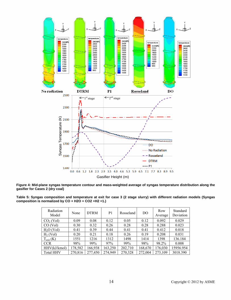
For the inner wall temperature shown in Fig. 3, the variation span (about 500K near the exit) is wider than the variation of syngas temperature. The non-radiation case has the highest value, whereas the P1 model case has the lowest wall temperature. The difference of wall temperature between these two cases is about 300K-500K. In the second stage, the S2S model gives a relatively uniform inner wall temperature when compared to other models. It appears that, when the radiation effect is included, both the syngas and wall temperatures decrease under the slurry coal gasification condition. 4.2 Case 2 (dry coal, 100%-0% for two stage injection) Case 2 is the two-stage oxygen-blown operation with dry coal distribution of 100%-0% between the first and the second stages. Syngas temperature and species mole fraction distributions at exit for different sub-cases are shown in Table


4. Similar to Case 1 (1 stage coal slurry), it is shown that the sub-cases with the none radiation, the P1 and the DO models have very similar results of syngas composition and temperature at the exit, while the results of the DTRM model and the Rosseland model yield noticeably different syngas compositions and produce very high exit syngas temperatures (400K-700K higher). Different from Case 1 with coal slurry, in the dry coal study of Case 2, the lower syngas exit temperatures predicted by the DO and P1 model could be caused by the slower forward WGS reaction rate than in the cases with Rosseland and DTRM models. Since water content in dry coal is much less than in the coal slurry, steam has not been sufficiently provided to promote forward WGS reaction to produce more H2 and CO2, so the results of syngas composition for P1 and DO models in Case 2 with more CO and less H2 are thought to be more reasonable than the sub-cases with DTRM and Rosseland models.

Figure 4 and Figure 5 provide contour and mass-weighted temperature distributions for both syngas and inner wall temperatures. It is interesting to see that the syngas temperature distributions predicted by the none radiation model, the P1 model, and the DO model are very consistent, while the DTRM model gives a higher syngas temperature (about 400K higher at the exit). The result of syngas temperature distribution for the Rosseland model is apparently not reasonable because it yields a very large and unrealistic swing of both syngas and wall temperatures along the gasifier.

For the inner wall temperature, the case with the DO model yields a similar result with the case without employing any radiation model. The wall temperature for P1 model is around 400K lower than it for DO model, while the temperature for DTRM model is about 300K higher than DO model. Note that in both the slurry coal and dry coal cases, P1 model predicts the lowest wall temperature. 4.3 Case 3 (coal slurry, 50%-50% for two stage injection) Case 3 is the two-stage oxygen-blown operation with dry coal distribution of 50%-50% between the first and the second stages. Syngas temperature and species mole fraction distributions at exit for different sub-cases are shown in Table 5. Syngas temperature and inner wall temperature distribution are shown in figures 6 and 7. Similar to Case 1, the Rosseland model gives uniform syngas temperature distribution, so this model does not work for gasification simulation. DO model, P1 model, DTRM model, and none radiation model have the same syngas temperature distribution with different levels. The combustion process is the main reaction at the first stage. The DO model yields the highest syngas temperature, while the P1 model continues to give the lowest syngas temperature; the maximum temperature difference between DO and P1 models is about 1000K between the first and second stage at around 2.5 m. Because 50% coal slurry is injected from second stage injection without oxygen, the gasification process dominates in the second stage; and, consequently, the syngas temperature drops drastically near the second stage injection location, as shown in Figure 6. The syngas temperature slightly increases at the second stage all the way to the exit of gasifier. This temperature increase may be caused by the exothermic process

from the WGS reaction in the second stage after coal slurry has been consumed completely.

At the second stage, the maximum wall temperature difference between the DO model and P1 model is about 300K. Different from the syngas temperature distribution, the inner wall temperature decreases from the first stage injection location (combustion area) all the way to the exit of gasifier. The case with the DTRM model predicts the highest inner wall temperature, while the P1 model continues to predicts the lowest one. The biggest temperature difference between these two models reaches an uncomfortably large value of approximately 1000K. 5.0 CONCLUSION Five different radiation models have been tested through three different operating conditions of gasification process. The results of syngas composition, syngas temperature, as well as the inner wall temperature in each case have been compared. The conclusions are the following:

a. Rosseland model does not yield reasonable and realistic results for gasification process. It either predicts an uncharacteristic nearly-constant syngas and wall temperature distributions along the gasifer for the slurry coal cases or a unreasonably large swing of temperature from very high to very low and back to very high value along the gasifier for the dry-coal feed case.

b. Inner wall temperature is more uniform in the case of S2S model than any other radiation models, since S2S model only considers the enclosure radiation transfer without including participating media.

c. The effect of radiation is much more significant in predicting the inner wall temperature than syngas temperature distribution.

d. The P1 model always predicts the lowest inner wall temperature in all the cases.

e. The DTRM model predicts very high syngas and wall temperatures in the dry coal feed case. In the one-stage coal slurry case, DTRM result is close to the S2S result. In this study, the various radiation models yield

uncomfortably large uncertainties in predicting syngas composition (18%), syngas temperatrure (21%), and wall temperature (28%). No solid conclusion can be derived from this study without a comparison with detailed experimental data consisting of local syngas composition and temperature information, as well as of the inner wall temperature distribution of the gasifier. However, it is fair to note that the Rosseland model does not seem to work reasonably well for simulating the gasification process. The P1 method seems to behave stably and is robust in predicting the syngas temperature and composition, but it seems to underpredict the gasifier’s inner wall temperature.


Table 3: Syngas composition and temperature at exit for case 1 (1 stage slurry) with different radiation models (Syngas composition is normalized by CO + H2O + CO2 +H2 =1.)

Radiation Model None DTRM P1 Rosseland DO S2S Average Standard

DeviationCO2 (Vol) 0.10 0.07 0.09 0.08 0.10 0.08 0.087 0.012 CO (Vol) 0.31 0.33 0.32 0.34 0.31 0.32 0.322 0.012 H2O (Vol) 0.39 0.42 0.40 0.39 0.39 0.42 0.402 0.015 H2 (Vol) 0.20 0.18 0.19 0.19 0.20 0.18 0.190 0.009 Texit (K) 1756 1415 1665 1500 1721 1480 1590 142.24 CCR 99% 97% 98% 99% 98% 98% 98% 0.008 HHV(kJ/kmol) 182,136 174,906 178,009 186,499 181,412 174,227 179,532 4705.67 Total HHV 272,809 280,556 278,650 279,890 275,986 279,171 277,844 2924.21

Gasifier Height (m)

Syn

gas

Tem

pera

ture

(K)

1st stage 2nd stage

Figure 2: Mid-plane syngas temperature contour and mass-weighted average of syngas temperature distribution along the gasifier for Cases 1 (coal slurry)


Gasifier Height (m)

Wal

l Tem

pera

ture

(K)

1st stage 2nd stage

Figure 3: Wall temperature contour and circumferential average of gasfier inner wall temperature distribution along the gasifier for Cases 1 (coal slurry) Table 4: Syngas composition and temperature at exit for case 2 (dry coal, 100%-0%) with different radiation models (Syngas composition is normalized by CO + H2O + CO2 +H2 =1.)

Radiation Model None DTRM P1 Rosseland DO Average Standard

DeviationCO2 (Vol) 0.06 0.10 0.05 0.10 0.07 0.076 0.023 CO (Vol) 0.53 0.51 0.53 0.48 0.52 0.514 0.021 H2O (Vol) 0.18 0.14 0.17 0.17 0.18 0.168 0.016 H2 (Vol) 0.23 0.25 0.23 0.26 0.23 0.24 0.014 Texit (K) 1733 2145 1747 2476 1770 1974 328.81 CCR 99% 97% 97% 99% 98% 98% 0.01 HHV(kJ/kmol) 230,941 229,188 230,658 235,206 233,943 231,987 2494.12 Total HHV 282,687 279,342 283,760 278,854 287,150 282,359 3406.295


Gasifier Height (m)

Syng

as T

empe

ratu

re (K

)

1st stage 2nd stage

Figure 4: Mid-plane syngas temperature contour and mass-weighted average of syngas temperature distribution along the gasifier for Cases 2 (dry coal) Table 5: Syngas composition and temperature at exit for case 3 (2 stage slurry) with different radiation models (Syngas composition is normalized by CO + H2O + CO2 +H2 =1.)

Radiation Model None DTRM P1 Rosseland DO Row

Average Standard Deviation

CO2 (Vol) 0.09 0.08 0.12 0.05 0.12 0.092 0.029 CO (Vol) 0.30 0.32 0.26 0.28 0.28 0.288 0.023 H2O (Vol) 0.41 0.39 0.44 0.41 0.41 0.412 0.018 H2 (Vol) 0.20 0.21 0.18 0.26 0.19 0.208 0.031 Texit (K) 1551 1216 1312 1498 1414 1398 136.184 CCR 98% 99% 97% 99% 98% 98.2% 0.008 HHV(kJ/kmol) 178,582 166,938 163,250 202,710 168,670 176,030 15956.954 Total HHV 270,816 277,450 274,949 270,328 272,004 273,109 3018.390


Gasifier Height (m)

Wal

l Tem

pera

ture

(K)

1st stage 2nd stage

Figure 5: Wall temperature contour and mass-weighted circumferential average of wall temperature distribution along the gasifier for Cases 2 (dry coal)


Gasifier Height (m)

Syng

as T

empe

ratu

re (K

)

1st stage 2nd stage

Figure 6: Mid-plane syngas temperature contour and mass-weighted average of syngas temperature along the gasifier for Cases 3 (Coal slurry, 50%-50%)

Gasifier Height (m)

Wal

l Tem

pera

ture

(K)

1st stage 2nd stage

Figure 7: Wall temperature contour and circumpherential average of inner wall temperature distribution along the gasifier for Cases 3 (Coal slurry, 50%-50%).


6.0 ACKNOWLEDGMENT This study was partially supported by the U.S. Department of Energy via a subcontract through Nicholls State University. 7.0 REFERENCES [1] Chen, C., Horio, M., and Kojima, T., 2000, “Numerical Simulation of Entrained Flow Coal Gasifiers”, Chemical Engineering Science, Vol.55, pp. 3861-3833. [2] Bockelie, M.J., Denison, K.K., Chen, Z., Linjewile, T., Senior, C.L., and Sarofim, A.F., 2002, “CFD Modeling For Entrained Flow Gasifiers in Vision 21 Systems,” Proceedings of the 19th Annual International Pittsburgh Coal Conference, Pittsburgh, PA. September 24-26, 2002. [3] Guenther, C., and Zitney, S.E., 2005, “Gasification CFD Modeling for Advanced Power Plant Simulation,” Proceedings of the 22th International Pittsburgh Coal Conference, Pittsburgh, Pennsylvania, September 12-15, 2005. [4] Chodankar, C.R., Feng, B., and Klimenko, A.Y., 2009, “Numerical Modeling of Underground Coal Gasification Process for Estimation of Product Gas Composition,” Paper 25-3, presented at the 26rd International Pittsburgh Coal-Gen Conference, Pittsburgh, Pennsylvania, Sept. 20-23, 2009. [5] Ajilkumar, A., Sundararajan, T., and Shet, U.S.P., 2009, “Numerical modeling of a steam-assisted tubular coal gasifier,” International Journal of Thermal Sciences, Vol. 48, pp. 308-321. [6] Wu, Y., Zhang, J., Smith, P., Zhang, H., Reid, C., Lv, J., and Yue, G., 2010, “Three-Dimensional Simulation for an Entrained Flow Coal Slurry Gasifier,” Energy Fuels, Vol. 24, pp. 1156–1163.

[7] Chen, M., 2010, “Numerical Simulation Analyses of an Entrained-bed Gasification Reactor,” Paper 45-4, presented at the 27th International Pittsburgh Coal Conference, Istanbul, Turkey, October 11 – 14, 2010. [8] Silaen, A., and Wang, T., 2005, “Simulation of Coal Gasification Process Inside a Two-Stage Gasifier,” Paper 20-1, Proceedings of the 22nd International Pittsburgh Coal Conference, Pittsburgh, Pennsylvania, September 19-22. [9] Silaen, A., and Wang, T., 2006, “Effect of Fuel Injection Angles on Performance of a Two-Stage Gasifier,” Paper 20-4, presented at the 23rd International Pittsburgh Coal-Gen Conference, Pittsburgh, Pennsylvania, Sept. 25-28, 2006. [10] Silaen, A., and Wang, T., 2011, “Investigation of Coal Gasification Process under Various Operating Conditions inside a Two-Stage Entrained Flow Gasifier”, accepted for publication in ASME Journal of Thermal Science and Engineering Applications, 2011. [11] Silaen, A., and Wang, T., 2010, “Effect of Turbulence and Devolatilization Models on Gasification Simulation,” International Journal of Heat and Mass Transfer, Vol. 53, pp. 2074-2091, 2010.

[12] Silaen, A., and Wang, T., 2009, “Comparison of Instantaneous, Equilibrium and Finite Rate Gasification Models in an Entrained Flow Coal Gasifier,” Paper 14-3, presented at the 26th International Pittsburgh Coal Conference, Pittsburgh, Pennsylvania, Sept. 21-24, 2009. [13] Lu, X., and Wang, T., 2011, “Water-Gas Shift Modeling in Coal Gasification in an Entrained-Flow Gasifier,” Paper 45-1, presented at the 28rd International Pittsburgh Coal-Gen Conference, Pittsburgh, Pennsylvania, Sept. 15-18, 2011.

[14] Wang, T., Silaen, A., Hsu, H.W., and Lo, M.C., 2006, “Partial Load Simulation and Experiments of a Small Coal Gasifier,” Paper 20-3, presented at the 23rd International Pittsburgh Coal-Gen Conference, Pittsburgh, Pennsylvania, Sept. 25-28, 2006. [15] Wang, T., Silaen, A., Hsu, H.W., and Shen, C.H., 2007, “Effect of Slag Tap Size on Gasification Performance and Heat Losses in a Quench-type Coal,” Paper 37-4, presented at the 24th International Pittsburgh Coal-Gen Conference, Johannesburg, South Africa, Sept. 10-14, 2007. [16] Wang, T., Silaen, A., Hsu, H.W., and Shen, C.H., 2010, “Investigation of Heat Transfer and Gasification of Two Different Fuel Injectors in an Entrained-Flow Gasifier,” ASME Journal of Thermal Science and Engineering Applications, Vol.2, pp. 011001/1-10, March 2010. [17] Wang, T., Silaen, A., Hsu, H.W., and Shen, C.H., 2011, “Top Fuel Injection Design in an Entrained-Flow Coal Gasifier Guided by Numerical Simulations,” ASME Journal of Thermal Science and Engineering Applications, Vol. 3, pp. 011009/1-8, March 2011. [18] Wang, T., Lu, X., Hsu, H.W., and Shen, C.H., 2011, “Investigation of the Performance of a Syngas Quench Cooling Design in a Downdraft Entrained-Flow Gasifier,” Paper 45-2, presented at the 28rd International Pittsburgh Coal-Gen Conference, Pittsburgh, Pennsylvania, Sept. 15-18, 2011. [19] Lockwood, F. C., and Shah, N.G., 1981, “A New Radiation Solution Method for Incorporation in General Combustion Prediction Procedures,” Eighteenth Symposium (International) on Combustion, The Combustion Institute, Pittsburgh, 1981, pp. 1405-1414.

[20] Chandrasekhar, S., 1950, Radiative Transfer, Oxford University Press, London. [21] Hottel, H.C., and Sarofim, A. F., 1967, Radiative Transfer, McGraw-Hill. [22] Grosshandler, W.L., 1980, “Radiative Heat Transfer in Non-homogeneous Gases: a Simplified Approach,” International Journal of Heat and Mass Transfer, Vol.23, pp. 1447-1459.


[23] Edwards, D.K., and Balakrishnan, A., 1973, “Thermal Radiation by Combustion Gases,” International Journal of Heat and Mass Transfer, Vol. 16, pp. 25-40. [24] Cumber, P.S., Fairweather, M., and Ledin, H.S., 1998, “Application of Wide Band Radiation Models to Non-homogeneous Combustion Systems,” International Journal of Heat and Mass Transfer, Vol. 11, pp. 1573-1584. [25] Sarofim, A.F., and Hottel, H.C., 1978, “Radiative Transfer in Combustion Chambers: Influence of Alternative Fuels,” in Proceedings of the Sixth International Heat Transfer Conference, Hemisphere, Washington, D.C., Vol.6, pp. 199-217. [26] Foster, P.J., and Howarth, C.R., 1968, “Optical constants of Carbon and Coals in the Infrared,” Carbon, Vol. 6, pp. 719-729. [27] Brewster, M.Q., and Kunitomo, T., 1984, “The Optical Constants of Coal, Char, and Limestone,” Journal of Heat Transfer, Vol. 106, pp. 678-683. [28] Viskanta, R., Ungan, A., and Menguc, M.P., 1981, “Predictions of Radiative Properties of Pulverized Coal and Fly-ash Polydispersions,” ASME paper no. 81-HT-24. [29] Buckius, R.O., and Hwang, D.C., 1980, “Radiation Properties for Polydispersions: Application to Coal,” ASME Journal of Heat Transfer, Vol. 102, pp. 99-103. [30] Grosshandler W.L., and Monteiro S.L.P., 1982, “Attenuation of Thermal Radiation by Pulverized Coal and Char,” Journal of Heat Transfer, Vol. 104, pp. 587-593. [31] Brewster, M.Q., and Kunitomo, T., 1984, “The Optical Constants of Coal, Char, and Limestone,” Journal of Heat Transfer, Vol. 106, pp. 678-683. [32] IM, K.H., and Ahluwalia, R.K., 1992, “Radiation Properties of Coal Combustion Products,” International Journal of Heat and Mass Transfer, Vol. 36, pp. 293-302. [33] Foster, P.J., and Howarth, C.R., 1968, “Optical Constants of Carbons and Coals in the Infrared,” Carbon, Vol. 6, pp. 719-729. [34] Lee, S.C., and Tien, C.L., 1981, “Optical Constants of Soot in Hydrocarbon Flames,” Eighteenth Symp. (Int.) on Combustion, Combustion Institute, Pittsburgh, pp. 1159-1166. [35] Smoot, D.L., and Smith, P.J., 1985, Coal Combustion and Gasification, Plenum Press. [36] Ranz, W.E., and Marshall, W.R., 1952, “Evaporation from Drops Part 1 and Part 2,” Chemical Engineering Progress, Vol. 48, pp. 173-180. [37] Fletcher, T.H., and Kerstein, A.R., 1992, “Chemical Percolation Model for Devolatilization: 3 Direct Use of 13C

NMR Date to Predict Effects of Coal Type,” Energy and Fuels, Vol. 6, pp. 414-431 [38] Fletcher, T.H., Kerstein, A.R., Pugmire, R.J., and Grant, D.M., 1990, “Chemical Percolation Model for Devolatilization: 2. Temperature and Heating Rate Effects on Product Yields,” Energy and Fuels Vol. 4, pp.54-60 . [39] Grant, D.M., Pugmire, R.J., Fletcher, T.H., and Kerstein, A.R., 1989, “Chemical Percolation of Coal Devolatilization Using Percolation Lattice Statistics,” Energy and Fuels, Vol. 3 pp. 175-186. [40] Kobayashi, H., Howard, J.B., and Sarofim, A.F., 1976, “Coal Devolatilization at High Temperatures”, 16th Symposium (International) on Combustion, 411-425. [41] Siegel, R., and Howell, J., 1980, Thermal Radiation Heat Transfer, Taylor & Francis. [42] Modest, M.F., 2003, Radiative Heat Transfer, Academic Press.

Documents

EFFECT OF RADIATION MODELS ON COAL …eccc.uno.edu/pdf/Lu-Wang radiation in gasification IMECE2012-86997.pdf · entrained flow gasifier developed for an IGCC process under ... Aspen