Effect of Price Reduction and Increased Service Frequency

Journal of Public Transportation, Vol. 20, No. 1, 2017 139

Effect of Price Reduction and Increased Service Frequency on

Public Transport Travel

Inge BrechanInstitute of Transport Economics, Oslo

Abstract

A random effects meta-analysis of the results from 15 projects involving price reduction and 9 projects involving increased service frequency showed that both price reduction and increased service frequency generated public transport travels. On average, the increased service frequency projects generated more travels by public transport than the price reduction projects. In the increased service frequency projects the proportion of travels generated by the increased frequency was strongly influenced by the size of the frequency increase. In the price reduction projects, we did not find a significant effect of the size of the price reduction on the proportion of travels generated by the price reduction. Finding that people’s use of public transport was related to the extent of the service offered suggests they have a need for transport that can be fulfilled with public transport. Although people appreciate lower fares in general, finding that use of public transport was not significantly related to the size of a price change suggests the effect of price change is uncertain.

Keywords: Price, service frequency, meta-analysis, travel mode choice, elasticity

Introduction

With the aim of generating more travel by public transport, several avenues may be considered. Two obvious options are to offer more service and to charge less for the service currently offered. Which of the two options brings the most success in terms of journeys generated? This research question is of interest to academia, policymakers, the public transport industry, environmental organizations, and general society. Research on longitudinal economic data (1987–1996) from France and England differ in their conclusions. Price elasticity was found to be greater than service (i.e., vehicle kilometers) elasticity in France, whereas the opposite was found in England (Bresson et al. 2003, 2004; Dargay and Hanly 2002). According to Preston (2014), research reviews

Effect of Price Reduction and Increased Service Frequency on Public Transport Travel


suggest that service elasticities in general are larger than price elasticities, but also that elasticities vary a lot. This paper investigated the research question by performing a meta-analysis of the results from customer survey data from the Norwegian trial scheme for public transport.

Use of Public Transport Related to Price and Service Frequency

At the most general level, use of public transport can be predicted by what customers give (i.e., cost) relative to what they get (i.e., service). Research on more specific factors associated with use of public transport are often related to fares (e.g., type of fare, price of petrol, income) and quality of service (e.g., intervals, reliability, interchanges) (see Balcombe et al. 2004). Although service quality may also include non-essential attributes, such as cleanliness, research has indicated that the problem-solving capability of the travel mode (i.e., taking people from where they are to where they want to go at the time they need to be there) is essential (Brechan 2006). Thus, routes and schedules are the primary service factors.

Results from meta-analyses on the effects of price and service frequency on use of public transport vary. Holmgren (2007) found average short-term service (vehicle kilometers) elasticity (1.05) to be more extreme than price elasticity (Europe -0.75 and America/ Australia -0.59). Holmgren (2007) found the service elasticity to vary more than the price elasticity. Hensher (2008) found average service (headway) elasticity (-0.29) to be less extreme than price elasticity (-0.40). Hensher (2008) found the price elasticity to vary more than the service elasticity. According to Paulley et al. (2006), the average short-term service elasticity (0.4) and price elasticity (-0.4) are similar in absolute strength. Paulley et al. (2006) concludes that there is a wide range of fare elasticities and suggests that the impact of prices is higher in the long run (vs. short run), in rural (vs. urban) areas, for leisure and shopping (vs. work and education) purposes and in off-peak (vs. traffic peak) hours. Similarly, they also suggest the impact of service (intervals) is higher in the long run (vs. short run), in rural (vs. urban) areas, and in off-peak (vs. traffic peak) hours.

Norwegian Trial Scheme for Public Transport

The Norwegian government’s Ministry of Transport established the Norwegian trial scheme for public transport in 1991, with the aim of developing public transport solutions that are more need-oriented, resource-efficient, and environmentally-friendly. Approximately 500 projects were awarded 461 million Norwegian kroner (NOK), the equivalent of approximately 60 million euro (EUR) or $70 million US, during the period 1991–1995. In total 24% of the projects were classified as route trials, including trials with increased service frequency, and 10% were classified as fare trials (i.e., trials with price reduction). Other projects in the trial scheme concerned bus terminals, information and marketing, ticketing, organization and administration, quality of vehicles, fuels, and telecommunication. Among the route and fare trials, 101 projects



were evaluated partly by means of an on-board customer survey. The results from these customer surveys constitute the data available for the current meta-analysis.

According to the database of Statistics Norway (www.ssb.no/statistikkbanken), the inland (excluding journeys starting or ending abroad) motorized passenger transport volume in Norway was 56,132 million passenger kilometres in 1995 (see Figure 1), which equals 35 km per person per day. This was divided among bus transport (7%), other road transport (81%—private car 78%, motorcycle 1%, taxi 1%, rental car 1%), rail (5%), air (6%), and sea (1%). Based on the Norwegian National Travel Study (www.toi.no/rvu) from 1992 and 1998, we estimated that people in Norway on average walked 1 km and bicycled 0.5 km per day in 1995. Thus, the non-motorized passenger travel volume was 1.5 km per person per day, compared to the motorized passenger travel volume of 35 km per person per day. There are large regional and seasonal differences. Norway is a sparsely-populated (14.29 pop. per sq. km in 1995) mountainous country (46% mountain, 43% forest, 6% lakes, 3% agriculture, 2% built) with a long coastline (25,148 km continental coastline) situated on the Arctic Circle, comparable in size to Poland, The Ivory Coast, Malaysia, or New Mexico. Most people in Norway live in cities on the coastline. Approximately 80% live in urban areas. Oslo, the capital, has a well-developed public transit system with a mix of buses, rail, and boats. All route and fare trials included in this meta-analysis took place in smaller cities (population < 150,000), where the public transit system consists of almost exclusively buses. Some of the areas have rail and/or boat service as well, but these travel modes make up only a very small part of the service. Rail’s share of passenger transport in Figure 1 stems mostly from regional and intercity train services not included in this meta-analysis, but one of the frequency trials involved a tram (trolley, streetcar) service.

FIGURE 1.Annual inland motorized

passenger transport volume in Norway

0

1,000

2,000

3,000

4,000

5,000

6,000

7,000

8,000

0

10,000

20,000

30,000

40,000

50,000

60,000

70,000

80,000

1965 1970 1975 1980 1985 1990 1995 2000 2005 2010

Popu

latio

n in

thou

sand

s

Mill

ion

pass

enge

r kilo

met

res

Sea and airRail

Bus

Road transport excl. bus

Population

Note: Includes only journeys starting and ending in Norway.



Method

The 101 customer surveys were fairly identical and included questions about the quality of public transport, travel behavior, and demographics. The questions measuring the direct impact of the price reduction or frequency increase were: “Are you aware of the recent changes in the ticket prices (or frequency of services)?” and, if so, “By what mode of transport would you have conducted this specific journey if the recent changes had not taken place?” The possible answers offered for the last question included all public modes of transport, private motorized modes of transport, non-motorized modes of transport, and the option of not traveling at all. The outcome variable included in this analysis is the proportion of respondents reporting that they were aware of the changes in the prices (or services) and that they would not have used public transport for this specific journey if the changes had not taken place.

Of the 101 projects, 12 were omitted due to very small survey sample (< 30 respondents) and another 12 were omitted because the projects were either quite unique (e.g., concerned boats rather than buses) or could not be exclusively categorized (e.g., included changes in prices as well as services). Among the remaining 77 projects, 25 were price reduction trials, 12 were increased frequency trials, and 40 were other route trials (mostly new routes). Finally, because some projects were merely continuations of earlier projects in the trial scheme and implied no further changes to the price or service, the final sample of price and frequency trials to be included in the meta-analysis consists of 15 price reduction trials and 9 increased frequency trials. All 24 trials took place in small cities (< 150,000 inhabitants), and all routes surveyed were general local bus routes (except one frequency trial that involved a tram service).

First, we calculated the average effect of each of the two groups of projects and compared the two to see if one type of project had a larger effect than the other. Then, we investigated the relationship between the outcome (i.e., proportion of journeys generated by the project) and the size of the change in price or frequency. The independent variables, price decrease and frequency increase, were measured as the price reduction in percent of the original fare and the increase in departures in percent of the original number of departures on a route.

Results

Information on the size of the price reduction or frequency increase, sample size of the customer surveys, and effect size discovered in the customer surveys are presented in Table 1 (price reduction projects) and Table 2 (service frequency increase projects). Effect sizes are presented as the number (labeled “raw effect”) of respondents reporting that they would not have used public transport for the current journey if the project (reduced price or increased frequency) had not taken place and the proportion (m) this number of respondents represents relative to the total number of people interviewed.



Project ID Region Price Reduction

Sample Size (n)

Raw Effect*

Proportion**

(m)

1-020 Østfold 30.00% 186 20 0.11

2-005 Akershus 33.33% 112 41 0.37

4-001A Hedmark 25.00% 114 37 0.32

4-001B Hedmark 25.00% 106 26 0.25

7-001 Vestfold 37.50% 270 29 0.11

9-001 Aust-Agder 18.60% 153 70 0.46

10-001 Vest-Agder 64.44% 514 238 0.46

10-002 Vest-Agder 22.22% 421 162 0.38

11-007 Rogaland 50.00% 404 89 0.22

11-009 Rogaland 36.36% 89 22 0.25

15-001 Møre og Romsdal 35.00% 805 230 0.29

15-002 Møre og Romsdal 34.21% 1125 324 0.29

15-015 Møre og Romsdal 35.00% 1955 707 0.36

18-001A Nordland 34.48% 90 26 0.29

18-001B Nordland 48.84% 90 46 0.51

Total 6434*Number of respondents reporting that journey was generated by price reduction.**Raw effect divided by sample size.

TABLE 2.Description of Projects

Involving Increase in Service Frequency

Project ID Region Frequency Increase

Sample Size (n)

Raw Effect*

Proportion**

(m)

7-005 Vestfold 67.83% 308 250 0.81

7-006 Vestfold 12.50% 235 105 0.45

10-018 Vest-Agder 42.58% 207 63 0.30

10-033 Vest-Agder 40.54% 166 77 0.46

10-036 Vest-Agder 44.44% 126 52 0.41

11-004 Rogaland 23.56% 143 39 0.27

11-027 Rogaland 45.56% 112 34 0.30

16-004 Sør-Trøndelag 26.98% 3494 329 0.09

16-009*** Sør-Trøndelag 9.32% 154 45 0.29

Total 4945* Number of respondents reporting that journey was generated by increase in service frequency.** Raw effect divided by sample size*** This trial involved tram (trolley, streetcar), whereas other trials involved buses.

We did not expect the effect sizes in the projects to be similar, because the projects differed with regard to the size of the price reduction or increase in service frequency implemented. As such, the effect sizes are not representations of a general fixed effect,

TABLE 1.Description of Projects

Involving Price Reduction



and, therefore, this is a meta-analysis of random effects (Shadish and Haddock 1994). In a fixed effects model, the effect sizes in the set of studies are all estimates of a common (i.e., fixed) effect in the population. Any difference between a study effect and the common effect would be due to sampling error, as a given study uses a sample of subjects from the population. The term “random effects” reflects the assumption that the effect sizes in a random effects meta-analysis are sampled from a larger population of effect sizes (Raudenbush 1994). We nevertheless started our analyses by investigating the homogeneity of the effect sizes.

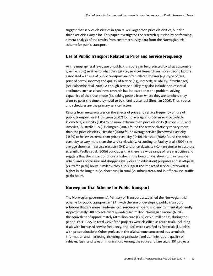
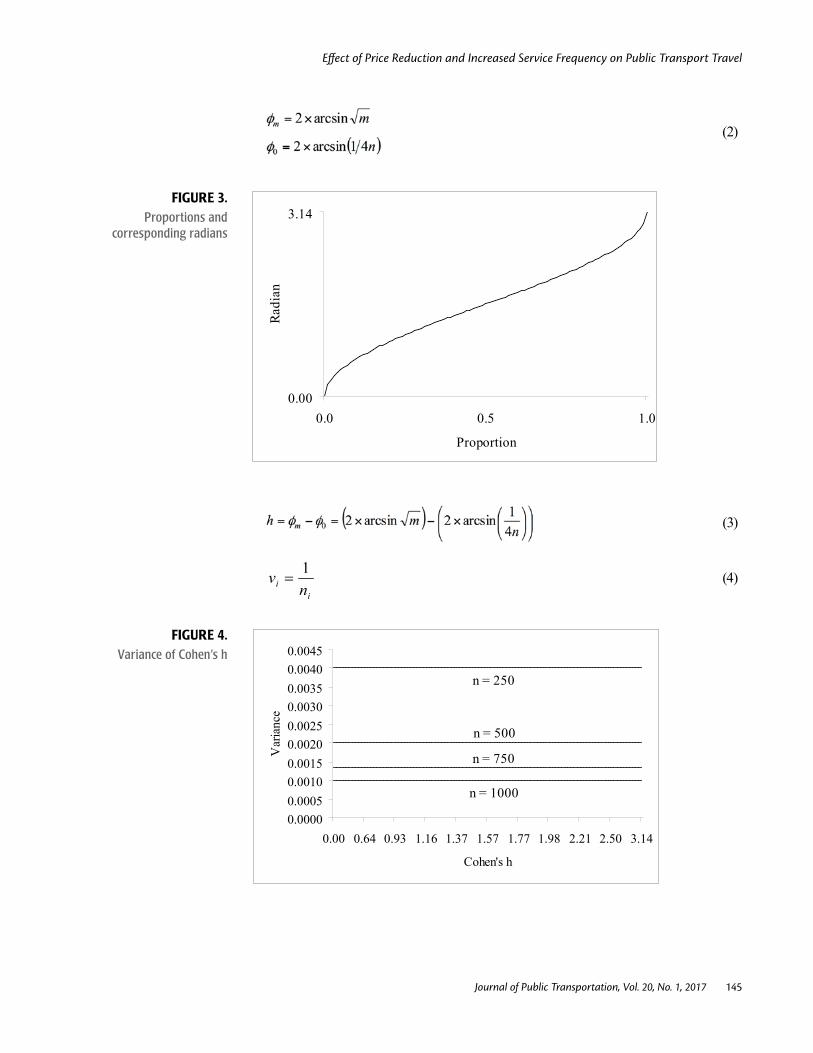
Because the variance (σ2) of a proportion (m) is determined in part by the magnitude of the proportion (see Equation 1 and Figure 2), proportions are not equally detectable, and the difference between proportions is not an appropriate measure of effect size (Cohen 1988). For example, at n = 250 and α = 0.05, the power to detect the difference between 0.1 and 0.2 is 0.89, whereas the power to detect the difference between 0.5 and 0.6 is 0.62 (Lenth 2004). Thus, we could not use proportions (or elasticities based on proportions) in our meta-analyses. Instead, we transformed the proportions to radians φ (see Equation 2, where n = sample size, and Figure 3) and calculated the effect size h representing the difference between a proportion and zero (see Equation 3) (Cohen 1988). The variance of the effect size h is not influenced by the magnitude of the effect size (see Equation 4 and Figure 4).

(1)

FIGURE 2.Variance of proportions

0.00000.00010.00020.00030.00040.00050.00060.00070.00080.00090.0010

0.0 0.1 0.2 0.3 0.4 0.5 0.6 0.7 0.8 0.9 1.0

Proportion

Var

ianc

e

n = 250

n = 500

n = 750

n = 1000



(2)

FIGURE 3. Proportions and

corresponding radians

0.00

3.14

0.0 0.5 1.0

Proportion

Radi

an

(3)

ii n

v 1= (4)

FIGURE 4.Variance of Cohen’s h

0.00000.00050.00100.00150.00200.00250.00300.00350.00400.0045

0.00 0.64 0.93 1.16 1.37 1.57 1.77 1.98 2.21 2.50 3.14

Cohen's h

Var

ianc

e

n = 250

n = 500

n = 750

n = 1000



When calculating the homogeneity test statistic (Q) (see Equation 5), the projects were weighted based on the within-study variance (vi) (see Equation 4) of the effect size ( ih ) (Shadish and Haddock 1994). Formulas for weights (wi) are given in Equation 6 (where k = number of studies).

∑

∑∑

=

=

=

−= k

ii

k

iiik

iii

w

hwhwQ

1

2

1

1

2 (5)

ii v

w 1= (6)

We used Equation 5 to calculate both overall homogeneity (QT) and the within-group (QWj) homogeneity for both types of projects. The input and computations regarding the price reduction projects are given in Table 1 (input) and Table 3 (computations), whereas the input and computations regarding the increased service frequency projects are given in Table 2 (input) and Table 4 (computations). To calculate the overall homogeneity (QT), we simply combined the numbers from Table 1 and Table 2 (input), and Table 3 and Table 4 (computations).

TABLE 3.Computational Details for

Projects Involving Price Reduction

Project ID Region h vi wi wihi wihi2

1-020 Østfold 0.67 0.0054 186 123.78 82.38

2-005 Akershus 1.30 0.0089 112 145.06 187.87

4-001A Hedmark 1.21 0.0088 114 137.70 166.33

4-001B Hedmark 1.03 0.0094 106 109.34 112.79

7-001 Vestfold 0.67 0.0037 270 179.81 119.74

9-001 Aust-Agder 1.48 0.0065 153 226.82 336.25

10-001 Vest-Agder 1.50 0.0019 514 768.85 1150.07

10-002 Vest-Agder 1.34 0.0024 421 562.93 752.70

11-007 Rogaland 0.98 0.0025 404 394.26 384.75

11-009 Rogaland 1.04 0.0112 89 92.12 95.35

15-001 Møre og Romsdal 1.13 0.0012 805 907.45 1022.93

15-002 Møre og Romsdal 1.13 0.0009 1125 1274.06 1442.86

15-015 Møre og Romsdal 1.29 0.0005 1955 2522.25 3254.10

18-001A Nordland 1.13 0.0111 90 101.64 114.79

18-001B Nordland 1.59 0.0111 90 142.87 226.80

Total 6434 7688.94 9449.72



Project ID Region h vi wi wihi wihi2

7-005 Vestfold 2.24 0.0032 308 690.61 1548.49

7-006 Vestfold 1.46 0.0043 235 343.59 502.36

10-018 Vest-Agder 1.17 0.0048 207 241.43 281.59

10-033 Vest-Agder 1.50 0.0060 166 248.24 371.23

10-036 Vest-Agder 1.39 0.0079 126 175.31 243.91

11-004 Rogaland 1.10 0.0070 143 156.65 171.60

11-027 Rogaland 1.16 0.0089 112 130.21 151.38

16-004 Sør-Trøndelag 0.62 0.0003 3494 2178.98 1358.89

16-009 Sør-Trøndelag 1.14 0.0065 154 175.40 199.77

Total 4945 4340.42 4829.22

The overall within-group homogeneity (QW) is the sum of the individual within-group homogeneity statistics (see Equation 7, where l = number of groups). The between-group homogeneity (QB) is the difference between the overall homogeneity statistic (QT) and the overall within-group homogeneity statistic (QW) (see Equation 8).

(7)

(8)

Calculations of homogeneity test statistics:

If the homogeneity statistic (Q) is larger than the upper-tail critical value of chi-square at k – 1 degrees of freedom, the observed variance in study effect sizes is significantly

TABLE 4.Computational Details for

Projects Involving Increase in Service Frequency



greater than what can be expected by chance. The results of the homogeneity test are presented in Table 5. The test revealed that overall the effect sizes were not homogenous. The effect sizes in the price reduction projects were not homogenous, nor were the effect sizes in the increased frequency projects. The test also indicated that there was a significant difference between the two groups of projects, but finding that the effect sizes within the groups are not homogeneous calls for a random effects analysis.

TABLE 5.Homogeneity

Q df pPrice reduction projects 261.07 14 <.01

Increased frequency projects 1019.47 8 <.01

Overall within groups 1280.54 22 <.01

Between groups 281.52 1 <.01

Overall 1562.06 23 <.01

Calculating the homogeneity test statistic had a purpose beyond investigating the homogeneity of the effects of the price reduction and frequency increase. In a random effects model the total variance ( ∗

iv ) of the effect of an individual study reflects both the within-study variance (vi) and the between-studies variance ( ). The relationship between the total variance ( ∗

iv ), the within-study variance (vi), and the between-studies variance ( ) is displayed in Equation 9. The within-group homogeneity test statistic (QWj) was used to estimate the between-studies variance ( ) for each of the two groups of projects (see Equation 10). When calculating the average effect size ( •h ) for each of the two groups of projects we weighed each individual effect size by its total variance rather than the within-study variance used in the homogeneity test. See Equation 11 regarding the average effect size ( •h ) and Equation 12 regarding weights ( ∗

iw ).

(9)

(10)

(11)

(12)



By completing the equations, we found the between-studies variance (see Table 6) and average effect size (see Table 7) for both types of projects. Computational details are presented in Table 8 (price reduction projects) and Table 9 (increased service frequency projects). Equation 13 gives the formula for calculating the total variance ( •v ) of the average effect size ( •h ), which was needed to calculate the confidence interval of the average effect size (see Equation 14) and for significance testing (see Equation 15 regarding a z-test of the average effect size). Equation 16 gives the formula for transforming the effect size ( •h ) back to a proportion ( •m ).

TABLE 6.Between-studies Variance

c

Price reduction projects 5418.75 0.0456

Increased frequency projects 2416.97 0.4185

(13)

(14)

α = .05 gives C.05 = 1.96

•

•=v

hz (15)

(16)

TABLE 7.Average Effects

m•h•

(95% CI*) v•z

(p)

Price reduction projects 0.301.16

(1.05-1.28)0.0034

19.94(<.01)

Increased frequency projects 0.37 1.31(0.88-1.73) 0.0471 6.03

(<.01)* CI = Confidence interval



Project ID Region wi2 vi wi wi

hi

1-020 Østfold 34596 0.0510 19.62 13.06

2-005 Akershus 12544 0.0545 18.34 23.75

4-001A Hedmark 12996 0.0544 18.39 22.22

4-001B Hedmark 11236 0.0550 18.17 18.75

7-001 Vestfold 72900 0.0493 20.28 13.51

9-001 Aust-Agder 23409 0.0521 19.18 28.44

10-001 Vest-Agder 264196 0.0475 21.03 31.46

10-002 Vest-Agder 177241 0.0480 20.85 27.87

11-007 Rogaland 163216 0.0481 20.80 20.30

11-009 Rogaland 7921 0.0568 17.60 18.21

15-001 Møre og Romsdal 648025 0.0468 21.35 24.07

15-002 Møre og Romsdal 1265625 0.0465 21.51 24.36

15-015 Møre og Romsdal 3822025 0.0461 21.69 27.98

18-001A Nordland 8100 0.0567 17.63 19.92

18-001B Nordland 8100 0.0567 17.63 27.99

Total 6532130 294.09 341.89

TABLE 8.Further Computational Details

for Projects Involving Price Reduction

TABLE 9.Further Computational Details for Projects Involving Increase

in Service Frequency

Project ID Region wi2 vi wi wi

hi

7-005 Vestfold 94864 0.4217 2.37 5.32

7-006 Vestfold 55225 0.4227 2.37 3.46

10-018 Vest-Agder 42849 0.4233 2.36 2.76

10-033 Vest-Agder 27556 0.4245 2.36 3.52

10-036 Vest-Agder 15876 0.4264 2.35 3.26

11-004 Rogaland 20449 0.4255 2.35 2.57

11-027 Rogaland 12544 0.4274 2.34 2.72

16-004 Sør-Trøndelag 12208036 0.4188 2.39 1.49

16-009 Sør-Trøndelag 23716 0.4250 2.35 2.68

Total 12501115 21.23 27.78

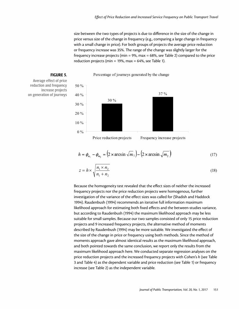
The difference between the average effect for the price reduction projects ( •m = 0.30) and the average effect for the increased frequency projects ( •m = 0.37) constituted a group difference of h = 0.15 that was highly significant (z = 7.72, p < .01). Thus, we can conclude that the increased frequency projects on average generated a larger proportion of journeys than the price reduction projects (i.e., 37% vs. 30%, see Figure 5). See Equation 17 for calculating the difference (h) between two proportions and Equation 18 for significance testing (z-test of the difference between two proportions). Note that the difference in effect size between the two groups of projects is not adjusted for difference in the size of price reduction or frequency increase. The impact of the size of the price reduction or frequency increase on journeys generated is evaluated later. There is, however, no indication that the difference in average effect

* * *

* * *



size between the two types of projects is due to difference in the size of the change in price versus size of the change in frequency (e.g., comparing a large change in frequency with a small change in price). For both groups of projects the average price reduction or frequency increase was 35%. The range of the change was slightly larger for the frequency increase projects (min = 9%, max = 68%, see Table 2) compared to the price reduction projects (min = 19%, max = 64%, see Table 1).

FIGURE 5. Average effect of price

reduction and frequency increase projects

on generation of journeys

Percentage of journeys generated by the change

30 %

37 %

0 %

10 %

20 %

30 %

40 %

50 %

Price reduction projects Frequency increase projects

(17)

21

21

nnnnhz

+×

×= (18)

Because the homogeneity test revealed that the effect sizes of neither the increased frequency projects nor the price reduction projects were homogenous, further investigation of the variance of the effect sizes was called for (Shadish and Haddock 1994). Raudenbush (1994) recommends an iterative full information maximum likelihood approach for estimating both fixed effects and the between-studies variance, but according to Raudenbush (1994) the maximum likelihood approach may be less suitable for small samples. Because our two samples consisted of only 15 price reduction projects and 9 increased frequency projects, the alternative method of moments described by Raudenbush (1994) may be more suitable. We investigated the effect of the size of the change in price or frequency using both methods. Since the method of moments approach gave almost identical results as the maximum likelihood approach, and both pointed towards the same conclusion, we report only the results from the maximum likelihood approach here. We conducted separate regression analyses on the price reduction projects and the increased frequency projects with Cohen’s h (see Table 3 and Table 4) as the dependent variable and price reduction (see Table 1) or frequency increase (see Table 2) as the independent variable.



We first conducted an ordinary least squares regression with the objective of finding an initial estimate of the between-studies variance ( ). We calculated the initial estimate of the between-studies variance ( ) by inserting the residual mean square (mean square error or MSE) from the regression into the formula presented in Equation 19. Then, we conducted a weighted least squares regression using weights ( ∗

iw ) calculated from the formula in Equation 12 based on the total variance ( ∗

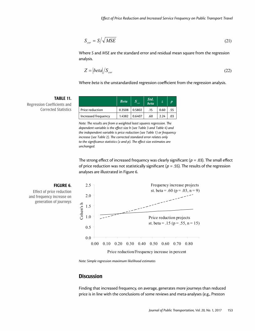
iv ) calculated from the formula in Equation 9. We used the residuals (res in Equation 20) of the first weighted least squares regression to re-estimate the between-studies variance ( ), using the formula presented in Equation 20. The re-estimate of the between-studies variance ( ) was then used to calculate weights (see Equation 12) for another weighted least squares regression. The process was repeated (iterated) until the estimates were essentially unchanged (i.e., converged). In our analyses, the estimates converged after the second iteration for both groups of projects, showing a strong (st. beta = .60) effect of frequency increase and a small effect (st. beta = .15) effect of price reduction. The results are presented in Table 10.

(19)

(20)

TABLE 10.Maximum Likelihood

Estimates

MSE† Beta Std. error*

Std. beta T* P*

Price reduction 0.0614 1.1516 0.3508 0.6226 .15 0.56 .58

Increased frequency 0.1072 1.2598 1.4382 0.7192 .60 2.00 .09

Note: The results (except between-studies variance ) are from a weighted least squares regression. The dependent variable is the effect size h (see tables 3 and 4) and the independent variable is price reduction (see Table 1) or frequency increase (see Table 2).* Uncorrected standard error yields incorrect significance statistics. The correction makes use of the residual mean square (MSE). See Table 11 for corrected statistics.

According to Hedges (1994) and Raudenbush (1994) the standard error used to calculate the significance of the weighted least square effect size must be corrected in meta-analyses. The formula for the corrected standard error is presented in Equation 21 and the formula for the significance test (z-test) of the effect size (i.e., unstandardized regression coefficient) is presented in Equation 22. The corrected standard errors, z-values, and significance statistics are presented in Table 11.



MSESScor = (21)

Where S and MSE are the standard error and residual mean square from the regression analysis.

corSbetaZ = (22)

Where beta is the unstandardized regression coefficient from the regression analysis.

TABLE 11.Regression Coefficients and

Corrected Statistics

Beta ScorStd. beta z p

Price reduction 0.3508 0.5802 .15 0.60 .55

Increased frequency 1.4382 0.6407 .60 2.24 .03

Note: The results are from a weighted least squares regression. The dependent variable is the effect size h (see Table 3 and Table 4) and the independent variable is price reduction (see Table 1) or frequency increase (see Table 2). The corrected standard error relates only to the significance statistics (z and p). The effect size estimates are unchanged.

The strong effect of increased frequency was clearly significant (p = .03). The small effect of price reduction was not statistically significant (p = .55). The results of the regression analyses are illustrated in Figure 6.

FIGURE 6.Effect of price reduction

and frequency increase on generation of journeys

0.0

0.5

1.0

1.5

2.0

2.5

0.00 0.10 0.20 0.30 0.40 0.50 0.60 0.70 0.80

Price reduction/Frequency increase in percent

Cohe

n's h

0.00 0.10 0.20 0.30 0.40 0.50 0.60 0.70 0.80

Frequency increase projectsst. beta = .60 (p = .03, n = 9)

Price reduction projectsst. beta = .15 (p = .55, n = 15)

Note: Simple regression maximum likelihood estimates

Discussion

Finding that increased frequency, on average, generates more journeys than reduced price is in line with the conclusions of some reviews and meta-analyses (e.g., Preston



2014; Holmgren 2007) and replicates the results from a longitudinal study in England (Dargay and Hanly 2002). It is also in line with Bresson et al. (2003), who suggest that structural differences in the French and English samples may account for the differences between England and France in their study. The data from France were gathered in urban areas only, whereas in England the data represent the entire country, including non-urban areas. The areas represented in our sample are mostly urban according to Norwegian standards, but more sparsely-inhabited when compared to French and English cities. Thus, our sample probably resembles the English sample more than the French sample with regard to the population density of the areas included. Also, the results from the French sample are less clear when looking at a longer period in time and including other indicators. The difference between price elasticity and service elasticity disappears when expanding the time period from 1987–1995 to 1975–1995 (Bresson et al. 2004). When using seat kilometers rather than vehicle kilometers, as a measure of service frequency the relationship shifts completely, so that service elasticity is larger than price elasticity (Bresson et al. 2004).

Finding that there is a strong relationship between the size of the frequency increase and the number of journeys generated is logical. If more departures mean more journeys, then even more departures should mean even more journeys, up to a point were lack of departures is no longer a barrier for choosing public transport. These results from Norway suggest people had a need for transport that could be satisfied with public transport. Although we do not believe the demand for transport is unlimited, the results support the “demand follows supply” hypothesis. If public transport service was increased, people used public transport more. If public transport service was increased more, people used it even more. Chen, Varley, and Chan (2011) came to a similar conclusion when investigating data on public transport between New York City and New Jersey from the period 1996 to 2009.

Not finding a significant relationship between the size of the price reduction and the number of journeys generated is puzzling. One possible explanation is that the price level of public transport in Norway was close to a level where price was no longer a barrier (i.e., very low price elasticity). Thus, a small price reduction may have been enough to reach that level, and any further reduction in prices may not serve any purpose. However, the changes in demand reported in this study does not suggest price elasticity is low. If we calculated a weighted (by sample size) average price elasticity based on the data from this study, it would be -.94, which is more extreme than the -.3 often used as a rule of thumb or the -.4 identified as average short term (1–2 years) price elasticity in another meta-analysis (Paulley et al. 2006). An alternative explanation is that any price reduction might have been considered favorably by part of the population, regardless of the size of the price reduction. This part of the population may report that choosing public transport was due to this positive event (i.e., the price reduction), a statement that may be correct or that may represent a positive attitude toward the event rather than a fact about their decision to travel by public transport. In either case, it may be the price reduction as an event and not the new price level that creates the extra journeys and/or the positive attitude. However, we did not find a fixed effect of the price reduction trials. The meta-analysis indicates great variation in the effects.



The heterogeneous effects of the price reduction projects in this meta-analysis suggest there is great uncertainty related to the outcome of price reductions. As such, this study joins the ranks of previous reviews and meta-analyses concluding there is large and unexplained variation in the effect of price changes.

The studies included in this meta-analysis have some methodological limitations. The data are from cross-sectional studies, in which travelers were asked what they have done if the changes in price or frequency had not taken place. A longitudinal study with measures taken before and after the change in price or frequency would have stronger validity. Although the participants de facto were traveling with public transport after the change in price or frequency, their former and alternative travel behavior was measured subjectively through self-reports. Future research should measure changes in travel behaviour longitudinally and with more objective measures (e.g., observation or documentation). Future research should also include information on the level of the price and service frequency before the change, as well as other information on the routes (e.g., route length, population density and socioeconomic characteristics of the area) that may explain the differences in the results.

Acknowledgment

This research was financially supported by the Research Council of Norway and the Norwegian government’s Ministry of Transport and Communication.

References

Balcombe, R., R. Mackett, N. Paulley, J. Preston, J. Shires, H. Titheridge, M. Wardman, and P. White. 2004. “The Demand for Public Transport: A Practical Guide,” TRL Report TRL593. Wokingham, UK: Transport Research Laboratory.

Brechan, I. 2006. “The Different Effect of Primary and Secondary Product Attributes on Customer Satisfaction.” Journal of Economic Psychology, 27: 441-458.

Bresson, G., J. Dargay, J.-L. Madre, and A. Pirotte. 2003. “The Main Determinants of the Demand for Public Transport: A Comparative Analysis of England and France Using Shrinkage Estimators.” Transportation Research Part A: Policy and Practice, 37: 605-27.

Bresson, G., J. Dargay, J.-L. Madre, and A. Pirotte. 2004. “Economic and Structural Determinants of the Demand for Public Transport: An Analysis on a Panel of French Urban Areas Using Shrinkage Estimators.” Transportation Research Part A: Policy and Practice, 38: 269-85.

Chen, C., D. Varley, and J. Chan. 2011. “What Affects Transit Ridership? A Dynamic Analysis Involving Multiple Factors, Lags and Asymmetric Behaviour.” Urban Studies, 48: 1893-1908.

Cohen, J. 1988. Statistical Power Analysis for the Behavioral Sciences, 2nd ed. Hillsdale, NJ: Lawrence Erlbaum Associates.



Dargay, J. M., and M. Hanly. 2002. “The Demand for Local Bus Services in England.” Journal of Transport Economics and Policy, 36: 73-91.

Hedges, L. V. 1994. “Fixed Effects Models.” In Cooper, H., and L. V. Hedges (eds.), The Handbook of Research Synthesis: 285-99. New York: Russell Sage Foundation.

Hensher, D. A. 2008. “Assessing Systematic Sources of Variation in Public Transport Elasticities: Some Comparative Warnings. Transportation Research Part A: Policy and Practice, 42: 1031-1042.

Holmgren, J. 2007. “Meta-analysis of Public Transport Demand.” Transportation Research Part A: Policy and Practice, 41: 1021-1035.

Lenth, R. 2004. Java Applets for Power and Sample Size. http://davidmlane.com/hyperstat/power.html.

Paulley, N., R. Balcombe, R. Mackett, H. Titheridge, J. Preston, M. Wardman, J. Shires, and P. White. 2006. The Demand for Public Transport: The Effect of Fares, Quality of Service, Income and Car Ownership. Transport Policy, 13: 295-306.

Preston, J. 2014. “Public Transport Demand.” In Nash, C. (ed.), Handbook of Research Methods and Applications in Transport Economics and Policy: 192-211. Cheltenham, UK: Edward Elgar.

Raudenbush, S. W. 1994. “Random Effects Models.” In Cooper, H., L. V. Hedges (eds.), The Handbook of Research Synthesis: 301-21. New York: Russell Sage Foundation.

Shadish, W. R., and C. K. Haddock. 1994. “Combining Estimates of Effect Size.” In Cooper, H., and L. V. Hedges (eds.), The Handbook of Research Synthesis: 261-81. New York: Russell Sage Foundation.

About the Author

Inge Brechan ([email protected]) is a senior lecturer in psychology at Inland Norway University of Applied Sciences. This research was conducted while he was senior research psychologist at the Institute of Transport Economics in Oslo. His research interests include transport psychology, consumer psychology, health psychology, and environmental psychology.

http://davidmlane.com/hyperstat/power.html

http://davidmlane.com/hyperstat/power.html

mailto:[email protected]

Documents

Effect of Price Reduction and Increased Service Frequency