Effect of model selection on computed water balance components

IRRIGATION AND DRAINAGE

Irrig. and Drain. 58: 492–506 (2009)

Published online 22 August 2008 in Wiley InterScience (www.interscience.wiley.com) DOI: 10.1002/ird.425

EFFECT OF MODEL SELECTION ON COMPUTED WATER BALANCECOMPONENTSy

RAJ KUMAR JHORAR1*, A. A. M. F. R. SMIT2 AND C. W. J. ROEST2

1Soil and Water Engineering, Chaudhary Charan Singh Haryana Agricultural University, Hisar, India2Alterra Green World Research, Department of Water and Environment, Environmental Science Group, Wageningen University and Research

Centre, Wageningen, The Netherlands

ABSTRACT

Soil water flow modelling approaches as used in four selected on-farm water management models, namely

CROPWAT, FAIDS, CERES and SWAP, are compared through numerical experiments. The soil water simulation

approaches used in the first three models are reformulated to incorporate an evapotranspiration process similar to

that used in SWAP. Computations are carried out for three soil types, representing sandy loam, loam and sandy clay

loam. The reformulated models are calibrated against simulation results obtained with SWAP. All the modelling

approaches predict nearly equal estimates of cumulative actual evapotranspiration for a wheat crop. When

compared with SWAP simulation results, the CERES type approach outperformed the other two approaches in

respect of estimated cumulative deep percolation losses. A new criterion is proposed to interpret simulation results

under deep water table conditions to suggest appropriate depth of water application. The resulting recommen-

dations for irrigation planning suggest that any of the modelling approaches may be used to suggest practical

irrigation considered in the present study. Copyright # 2008 John Wiley & Sons, Ltd.

key words: scheduling index; soil water modelling approaches; water balance; irrigation; deep percolation

Received 3 July 2007; Revised 5 March 2008; Accepted 6 March 2008

RESUME

Les modeles representant l’eau dans le sol selon quatre pratiques de gestion de l’eau au champ, soit CROPWAT,

FAIDS, CERES et SWAP sont compares numeriquement. Les simulations de l’eau du sol utilisees dans les trois

premiers modeles sont reformulees pour incorporer un processus d’evapotranspiration semblable a celui utilise

dans SWAP. Des calculs sont effectues pour trois types de sols representant les limons sableux, le limons et les

limons sablo-argileux. Les modeles reformules sont calibres avec des resultats de simulation obtenus avec SWAP.

Tous les modeles prevoient des evaluations presque egales de l’evapotranspiration reelle cumulee pour une culture

de ble. En comparant avec les resultats de simulation SWAP, le modele CERES a surpasse les deux autres modeles

pour l’estimation des pertes par percolation profonde cumulees. Un nouveau critere d’interpretation des resultats

dans des conditions d’aquifere profond est propose pour suggerer la dose d’eau appropriee. Il en resulte

des recommandations pour le pilotage de l’irrigation indiquant que chacun des modeles peut etre utilise pour

representer les pratiques d’irrigation considerees dans la presente etude. Copyright # 2008 John Wiley & Sons,

Ltd.

mots cles: index de pilotage; modelisation de l’eau dans le sol, bilan hydrique, irrigation, percolation profonde

*Correspondence to: Raj Kumar Jhorar, Department of Soil andWater Engineering, CCSHaryana Agricultural University, Hisar 125 004, India.E-mail: [email protected] du choix du modele sur les composantes du bilan hydrique calcule.

Copyright # 2008 John Wiley & Sons, Ltd.

COMPUTED WATER BALANCE COMPONENTS 493

INTRODUCTION

We are living in an era of increasing water scarcity due to growing competition for good-quality water between

agricultural and non-agricultural sectors. Approximately 80% of all the available fresh water supply is being used

for agriculture and food production. The efficiency of water in agricultural production is, however, low. Only

40–60% of the water is effectively used by the crops (Smith, 1996). Poor management of irrigation water at field

level is one of the reasons for this low water use efficiency in irrigation. The present situation underlines the

necessity to effectively and productively manage the limited water resources while maintaining or even improving

the environment.

Irrigation scheduling, the process to decide depth and timing of water application, is the key to improving

performance of irrigation systems at field level. However, the development of appropriate irrigation schedules,

under the present situation where a range of environmental problems such as waterlogging and salinisation are

linked to inefficient water use, requires quantification of different water and salt balance components associated

with alternative schedules. To determine these components, we need more sophisticated technologies to observe

and to measure, from which we may infer guidelines for improving irrigation water management. General

guidelines for irrigation scheduling are inherently difficult to formulate because of spatial variability of related

agro-geo-hydrological parameters. Location-specific guidelines can be formulated, provided all possible strategies

are monitored extensively in the field. Unfortunately, however, this option is expensive, time consuming and

difficult to implement under all situations. Consequently, there is a need to adopt alternative means of developing

irrigation schedules, including simulation models to perform the soil water balance using soil, crop and

meteorological data.

Simulation is an imprecise technique (Rubinstein, 1981; Silberstein, 2006). All that is required is that there be a

high correlation between prediction by the model and what would actually happen with the real system. The

purpose of a simulation model is to enable the analyst to determine how one or more changes in various aspects of

the modelled system may affect other aspects of the system or the system as a whole. Despite some deficiencies in

absolute model predictions, proper interpretation of model results makes modelling a powerful tool in solving a

variety of practical field problems (Kabat and Feddes, 1995).

The art of simulation modelling has grown rapidly over the last two decades and application studies are

expanding worldwide (Kabat et al., 1995). This is in recognition of the need to develop practical solutions for

various water management related problems such as irrigation scheduling, design of tile drainage system and

conjunctive use planning. Knowing that a simulation model (however complex it may be) is a simplified

reproduction of reality, it would be worthwhile to examine the relative credibility of different models so as to help

one to select a particular model under the prevailing conditions in the area of interest. Avast number of models have

appeared in the field of water management (Van den Broek, 1996). These vary from field-scale models to

regional-scale models involving different levels of complexity in their formulation. The study reported in this paper

assesses the reliability and applicability of some of the common soil water balance modelling approaches for

irrigation planning at the field level. The problem is not the availability of models but much more the level of

complexity desired to obtain reliable solutions.

In this study, four soil water flow modelling approaches as used in field-scale studies are compared. Cumulative

water balance components as predicted by different models are evaluated. It is also investigated how the final

recommendations for water application are affected by model choice. The main objective of this study is to

investigate the relative performance of different concepts of soil water flow simulation as used in the formulation of

on-farm water management models.

MODELLING APPROACHES

Several approaches are used for simulating the soil water balance. Answers to most of the on-farm irrigation

planning problems could be arrived at by quantifying and analysing different water and salt balance components in

one dimension (vertical) only. Therefore, the analysis and modelling examples in this paper are restricted to

one-dimensional vertical flow cases.

Copyright # 2008 John Wiley & Sons, Ltd. Irrig. and Drain. 58: 492–506 (2009)

DOI: 10.1002/ird

494 R. K. JHORAR ET AL.

The simplest modelling approach (CROPWAT: Smith, 1992) is based on the hypothesis that soil water storage

capacity is determined by the classical concept of field capacity. The amount of water held by a soil between field

capacity and wilting point in the root zone is considered as available to plants. Precipitation/rainfall in excess of the

quantity required to recharge soil moisture to field capacity is considered as deep percolation. Another approach

(CERES: Ritchie, 1972) defines soil water storage capacity by the saturation capacity of the soil. It is assumed that

water stored between saturation and field capacity can also be used by the plants. However, water stored between

saturation and field capacity is considered to drain at a rate determined by drainage rate parameter, designated as

SWCON.Water draining below the root zone is considered as percolation loss and unavailable to plants by both the

CROPWATand CERES approaches. In the above two approaches, water from upper to lower layer can only flow if

it is in excess of the storage capacity of the upper layer. Yet another modelling approach (FAIDS: Roest et al.,

1993), although based on the classical concept of field capacity, redistributes irrigation water to different soil layers

in proportion to moisture deficit in the layers. However, in the case of rainfall, water from upper to lower layer can

only flow if it is in excess of the storage capacity of the upper layer. In the FAIDS model a certain amount of water

stored in the deeper layers is also considered to be available to plants. In addition to thewater stored in the root zone,

50% of the water stored in a predefined depth located below the root zone (referred to as depth of capillary zone,

Dc), is considered available for plants.

All the above approaches neglect possible slow drainage below field capacity. Realising that soil water dynamics

is a very complex process, depending among others on soil hydraulic properties, upper and lower boundary

conditions, other kinds of models (SWAP: Van Dam et al., 1997; HYDRUS: Vogel et al., 1996; and many others)

are based on the numerical solution of the Darcy-Richards (D-R) equation. The D-R equation, extended by a sink

term to account for root water uptake, gives a full parameterisation of the one-dimensional soil water flow in

unsaturated soil and up to now has been used as the basic mathematical expression that underlies unsaturated flow

phenomena (Feddes et al., 1988).

In addition to the difference in basic flow principles as described above, diverse approaches are adopted for other

involved processes such as root water uptake. The performance of different simulation models is expected to be

dependent upon the formulation of soil–water–plant–atmospheric relationships. It is therefore imperative to study

the relative performance of different soil water flow approaches under similar conditions to judge the reliability of

their predictive capability. Four different soil water flow modelling approaches, as used in CERES, CROPWAT,

FAIDS and SWAP, are considered for this study.

METHODOLOGY

Model formulation

One of the options available for this study was to use the original versions of the selected models (CROPWAT,

CERES, FAIDS and SWAP) and compare their relative performance. SWAP and CERES simulate crop growth

differently, and FAIDS and CROPWAT require crop growth to be known in advance. Differences in crop growth

may affect the simulation results, making it difficult to quantify the exact role of the employed soil water flow

hypothesis on different water balance components. Moreover, the selected models also differ in the way

evapotranspiration (ET) is simulated. With testing of different concepts of soil water flow simulation as the basic

objective, it was considered more appropriate to reformulate different modelling approaches. We used the original

formulation of SWAP. The soil water flow processes as adopted in CROPWAT, CERES and FAIDS were

reformulated and are designated respectively as CROPWAT(A), CERES(A) and FAIDS(A), where A stands for the

approach used in this study. Daily values of potential transpiration Tp (mm d�1) and potential evaporation Ep

(mm d�1) as obtained in SWAP are input to these reformulated models. Actual evaporation Ea (mm d�1) is

estimated in a similar manner to Black’s approach (Black et al., 1969):

Copyri

Ea ¼ m �ffiffiffiffiffiffiffitdry

p�

ffiffiffiffiffiffiffiffiffiffiffiffiffiffiffitdry � 1

p� �(1)

where m is the parameter characterising the evaporation process and tdry is the time (days) since the soil was last

wetted. It was further assumed that the top 30 cm of the soil contribute towards evaporation. The parameter m was

ght # 2008 John Wiley & Sons, Ltd. Irrig. and Drain. 58: 492–506 (2009)

DOI: 10.1002/ird


adjusted to obtainEa values close to those obtained with SWAP. Actual transpiration Ta (mm d�1) was estimated in a

similar manner to the approach followed in SWAP (Feddes et al., 1978), with the difference that Tp was not

distributed among different layers. SWAP uses a semi-empirical approach to describe soil moisture uptake by roots.

The effect of moisture content on Ta is accounted for through a reduction factor b. The average moisture content in

the root zone was used to determine the reduction factor b. This approach was adopted for the following reasons:

when comparing the SWAP type model with the CROPWAT or FAIDS type approach, it seems more suitable to

make any judgement based on total moisture simulated rather than soil moisture distribution along the profile.

Moreover, the original formulation of CROPWAT is a single-layer model and FAIDS uses whole profile moisture

content to calculate actual evapotranspiration, ETa (mm d�1). A common flow diagram for the CROPWAT(A),

CERES(A) and FAIDS(A) is shown in Figure 1.

Simulation procedure

One way to judge the reliability of different models based on different concepts is to compare the ability of these

models to reproduce known field experimental observations. In this process, uncertain model parameters

are adjusted until the deviation between simulated and observed results is minimal. However, this has the

disadvantage that the findings regarding the comparative performance of the models may be valid only for the

experimental conditions, e.g. soil type and irrigation regimes. In this study, simulations are carried out for three soil

types to determine different water balance components for a wheat crop under different irrigation regimes. The

cumulative water balance components are used to decide on the appropriate depth of water application. The soil

hydraulic properties of the three soils, representing sandy loam, loam and clay loam, are given in Table I.

The selected models are used to develop practical irrigation schedules under canal water supply constraints

experienced in north India. The farmers in canal-irrigated areas of northwest India generally receive their irrigation

water on a fixed rotation basis known as warabandi. It is a system of equitable water distribution by turns according

to a predetermined schedule specifying the day, time and duration of supply to each irrigator in proportion to land

holding in the outlet command (Singh et al., 2006). Since the surface method of irrigation is most prevalent on

Indian farms, it is also not practical (if the system is to be operated efficiently) to vary depth of applied water from

one irrigation event to another. Accordingly, the irrigation scheduling criterion studied in this paper is that of fixed

irrigation of appropriate depth at pre-decided dates. This implies that the appropriate depth of water application is

the only variable that remains to be decided given the dates on which water is available. For the present simulation

study, the recommended irrigation calendar (Table II) is followed to determine the appropriate depth of water

application for different irrigation options.

For each of the three irrigation options, the depth of water application is varied from 4 to 10 cm at each irrigation

event. In the following sections, the different irrigation treatments are referred as Indm, where In and dm represent the

number of irrigation gifts and depth (cm) of application, respectively. Following this designation, I4d4 represents

irrigation treatment with four irrigations (I4) and 4 cm depth (d4) of application at each of the four irrigations.

Likewise, I6d10 represents irrigation treatment with six irrigations (I6) and 10 cm depth of application at each of the

six irrigations.

Actual evapotranspiration (ETa), deep percolation (DP) and change in soil moisture storage (DS) for alternative

strategies are computed by the different simulation models. It is assumed that no losses occur due to surface runoff.

The resulting water balance components as simulated by the selected modelling approaches and the subsequent

inferences drawn are compared to evaluate the reliability of different modelling approaches.

Model evaluation procedure

First, the cumulative ETa and DP values as predicted by CROPWAT(A), CERES(A), FAIDS(A) and SWAP are

compared. Next, various water balance components (i.e., ETa, DP, amount of irrigation I and precipitation P) are

used for alternative scenarios to suggest an appropriate irrigation application depth. The effect of the choice of

model on the final recommendations is examined. Since subjective procedures may lead to a biased decision,

particularly when comparing different models, a preferred method is to base the recommendations on some


DOI: 10.1002/ird

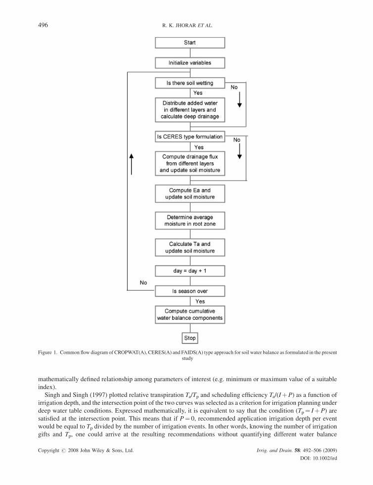
Figure 1. Common flow diagram of CROPWAT(A), CERES(A) and FAIDS(A) type approach for soil water balance as formulated in the presentstudy


mathematically defined relationship among parameters of interest (e.g. minimum or maximum value of a suitable

index).

Singh and Singh (1997) plotted relative transpiration Ta/Tp and scheduling efficiency Ta/(IþP) as a function of

irrigation depth, and the intersection point of the two curves was selected as a criterion for irrigation planning under

deep water table conditions. Expressed mathematically, it is equivalent to say that the condition (Tp¼ IþP) are

satisfied at the intersection point. This means that if P¼ 0, recommended application irrigation depth per event

would be equal to Tp divided by the number of irrigation events. In other words, knowing the number of irrigation

gifts and Tp, one could arrive at the resulting recommendations without quantifying different water balance


DOI: 10.1002/ird

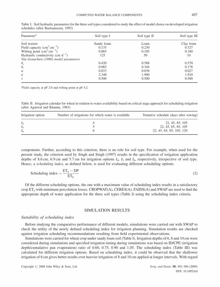
Table I. Soil hydraulic parameters for the three soil types considered to study the effect of model choice on developed irrigationschedules (after Bastiaanssen, 1993)

Parametera Soil type I Soil type II Soil type III

Soil texture Sandy loam Loam Clay loamField capacity (cm3 cm�3) 0.135 0.230 0.327Wilting point (cm3 cm�3) 0.065 0.105 0.180Hydraulic conductivity (cm d�1) 125 50 10Van Genuchten (1980) model parametersus 0.420 0.588 0.570ur 0.065 0.104 0.178a 0.033 0.038 0.027n 2.340 1.990 1.910l 0.500 0.500 0.500

aField capacity at pF 2.0 and wilting point at pF 4.2.

Table II. Irrigation calendar for wheat in relation to water availability based on critical stage approach for scheduling irrigation(after Agarwal and Khanna, 1983)

Irrigation option Number of irrigations for which water is available Tentative schedule (days after sowing)

I4 4 22, 45, 85, 105I5 5 22, 45, 65, 85, 105I6 6 22, 45, 65, 85, 105, 120


components. Further, according to this criterion, there is no role for soil type. For example, when used for the

present study, the criterion used by Singh and Singh (1997) results in the specification of irrigation application

depths of 8.6 cm, 6.9 cm and 5.7 cm for irrigation options I4, I5 and I6, respectively, irrespective of soil type.

Hence, a scheduling index, as defined below, is used for evaluating different scheduling options:

Copyri

Scheduling index ¼ ETa � DP

ETp

(2)

Of the different scheduling options, the one with a maximum value of scheduling index results in a satisfactory

crop ETa with minimum percolation losses. CROPWAT(A), CERES(A), FAIDS(A) and SWAP are used to find the

appropriate depth of water application for the three soil types (Table I) using the scheduling index criteria.

SIMULATION RESULTS

Suitability of scheduling index

Before studying the comparative performance of different models, simulations were carried out with SWAP to

check the utility of the newly defined scheduling index for irrigation planning. Simulation results are checked

against irrigation scheduling recommendations resulting from field experimental observations.

Simulations were carried for wheat crop under sandy loam soil (Table I). Irrigation depths of 6, 8 and 10 cmwere

considered during simulations and specified irrigation timing during simulations was based on ID/CPE (irrigation

depth/cumulative pan evaporation) ratio of 0.60, 0.75, 0.90 and 1.05. The scheduling index (Table III) was

calculated for different irrigation options. Based on scheduling index, it could be observed that the shallower

irrigation of 6 cm gives better results over heavier irrigation of 8 and 10 cm applied at longer intervals. With regard

ght # 2008 John Wiley & Sons, Ltd. Irrig. and Drain. 58: 492–506 (2009)

DOI: 10.1002/ird

Table III. Simulation (SWAP)-based scheduling index for wheat crop on a sandy loam soil in relation to different irrigationoptions

Irrigation depth (cm) ID/CPE ratio

0.60 0.75 0.90 1.05

6 0.62 0.72 0.77 0.748 0.53 0.59 0.68 0.6710 0.56 0.51 0.57 0.32


to timing of irrigation, the best performance is expected to occur when the 6 cm irrigation water is scheduled to

synchronise with an ID/CPE ratio of 0.9 rather than at 0.6, 0.75 and 1.05 ratios. Based on three years of field

experiments for wheat crop with similar irrigation treatments on a sandy loam soil, Agarwal and Khanna (1983),

while using observed yields and water production efficiency, came to the same conclusions. This verification

showed that the concept of scheduling index is an acceptable criterion to generate practical irrigation schedules.

Model calibration

Since the soil hydraulic parameters as used in SWAP are known (Table I), simulations were carried out with

SWAP to generate reference numerical experiments. The other three models (i.e., CROPWAT(A), CERES(A) and

FAIDS(A)) were then calibrated to determine representative soil parameter as used in these models. All three

models were calibrated to reproduce water balance components obtained for most dry (I4d4) and wet (I6d10)

irrigation treatment. One of the options was to select the treatment I5d7 for calibration, which is in the middle range

of all the irrigation options studied in the present study. The irrigation treatment I5d7 results in no percolation loss

(as simulated by SWAP) for soil types II and III. The information on percolation loss is required to determine the

drainage rate parameter SWCON for the CERES(A) model. Simulations with SWAP for I5d7 results in Ta being

equal to Tp. FAIDS(A) requires that the depth of capillary zone Dc be determined in such a way that the role of the

capillary zone is clearly evident and this happens when moisture deficit is maximal, e.g. treatment I4d4 in our case.

Considering these points DP loss as simulated by SWAP for I6d10 and theETa for I4d4 were the governing criteria for

calibrating the CROPWAT(A), CERES(A) and FAIDS(A). It is assumed that wilting point, corresponding to

pF¼ 4.2, represents the lower limit of available water. For CROPWAT(A), the only parameter to be determined is

the moisture content at field capacity. The best results with CERES(A) are obtained when field capacity is fixed

corresponding to pF¼ 2.0 for all the three soils. This means that SWCON is the only uncertain parameter to be

estimated by calibration. FAIDS(A) requires both field capacity and Dc as the calibrating parameters. We selected

I5d7 treatment for validation. The simulated water balance components for the I5d7 irrigation treatment, along with

relevant model parameter, are given in Table IV.

Simulated water balance components

Actual evapotranspiration. ETa as simulated by different models for the three soil types (Table I) and

irrigation options (Table II) studied is compared in Figure 2. All the models predict similar trends of ETa for

increasing depth of water application. However, some under- and over-predictions of ETa by CROPWAT(A),

CERES(A) and FAIDS(A) as compared to SWAP are to be noted.

Soil type I. The ETa predicted by different models is quite similar except for the consistent over-prediction by

FAIDS(A) for irrigation option I4. The over-prediction is attributed to the contribution from the capillary zone as

formulated in the FAIDS approach. The contribution from lower layers (capillary zone) in response to moisture

deficit in the root zone may undoubtedly occur. This is also demonstrated by the fact that the ETa as predicted by


DOI: 10.1002/ird

Table IV. Validation results of CROPWAT(A), CERES(A) and FAIDS(A) against SWAP for the three soil types and I5d7irrigation treatment

Model Soil type Water balance components (cm) Model parameters

ETa DP DS ufc SWCON/Dc

Reference-SWAP I 33.2 5.0 3.1 — —II 39.2 0.0 4.2 — —III 39.6 0.0 4.6 — —

CROPWAT(A) I 32.7 4.8 2.5 0.164 —II 39.0 0.0 4.0 0.300 —III 39.6 0.0 4.6 0.414 —

CERES(A) I 32.9 4.8 2.7 0.134 0.72a

II 39.0 0.0 4.0 0.229 0.57a

III 39.6 0.0 4.6 0.327 0.49a

FAIDS(A) I 33.8 5.0 3.8 0.152 47.0b

II 39.3 0.0 4.3 0.285 47.0b

III 39.6 0.0 4.7 0.393 33.0b

aSWCON.bDc (cm).


CROPWAT(A) and CERES(A) for I4d4 could not be further increased during calibration to bring it on a par with

that of SWAP. With no DP losses for I4d4 treatment, the only reason for the ETa under-prediction, though slight, by

CROPWAT(A) and CERES(A) is the neglect of any upward flow from the lower layers in these models. An account

of net flow across the bottom of the root zone for I4d4 treatment showed that SWAP simulated an upward flow of

6.4mm for the growing season of 140 days. In reality, the capillary zone may contribute to response to moisture

deficit in the bottom layer of the root zone. On the other hand, the approach used in FAIDS determines capillary

zone contribution in response to moisture deficit in the entire root zone. This results in over-prediction of capillary

zone contribution, and hence over-prediction in ETa by the FAIDS approach. For the other two schedules, the

predicted ETa by all the models is quite similar.

Soil type II. The unattainable gap in ETa by CROPWAT(A) and CERES(A) as compared to SWAP for I4d4(calibration treatment) is comparatively larger than in soil type I. Again, no DP loss for I4d4 by any of the models

indicates that the contribution from lower layers is responsible for higher ETa as predicted by SWAP and FAIDS(A).

Further, an account of net flow across the bottom of the root zone, as simulated by SWAP for I4d4 treatment, showed

an upward flow of 14.1mm for the growing season. A comparatively larger value of upward flow than that observed

for soil type I (6.4mm) points to the significance of lower layers in such soils when moisture deficit develops in the

root zone. Therefore, the CROPWATand CERES type models may underestimate ETa for dryland conditions. The

over-prediction of ETa by FAIDS(A) has the same explanation as discussed for soil type I.

The excellent match between predicted ETa for heavier depth of application is due to the attainment of near

potential values for these treatments. Prediction of higher ETa by CROPWAT(A), CERES(A) and FAIDS(A) than

SWAP for I6d5 and I6d6 is attributed to the approach adopted to simulate Ta. In case of SWAP, Tp is distributed to

different root zone layers and Ta is calculated based on the layer-wise moisture status. If the total amount of water

stored in the whole profile, between two irrigation events, is sufficient to meet potential demand, the approach

adopted in SWAP may still simulate Ta< Tp. This is due to the fact that applied water takes time to reach different

layers. For example, on an irrigation day, particularly for heavy soils, SWAP may simulate moisture distribution

such that upper layers are above field capacity and lower layers are still deficient in moisture. This moisture

distribution means that the Ta from lower layers may be less than the assigned Tp to these layers. On the other hand,

the approach used in other models instantly distributes irrigation water to the whole profile and thus Ta will be equal

to Tp. In reality, the instant recharge of different layers may be questionable for such soils.


DOI: 10.1002/ird

Figure 2. Actual evapotranspiration (ETa) as simulated by different modelling approaches. I4, I5 and I6 denote irrigation options with four, fiveand six irrigation events, respectively. Indicated irrigation depths are for each irrigation event


DOI: 10.1002/ird



Soil type III. The unattainable gap between ETa by CROPWAT(A) and CERES(A) as compared to SWAP is

similar to that of soil type II. An account of net flow across the bottom of the root zone, as simulated by SWAP for

I4d4 treatment, showed an upward flow of 15.4mm for the growing season. This indicates that the contribution from

lower layers is maximal in heavy soils (soil type III). Other aspects of ETa predictions are similar to those of soil

type II.

Deep percolation loss. The net downward flow occurring at the bottom of the root zone for SWAP and

FAIDS(A) is considered as deep percolation: DP loss. The total downward flow below the root zone is considered as

deep percolation loss for CERES(A) and CROPWAT(A). The DP as simulated by different models is compared in

Figure 3. In contrast to the almost equivalent behaviour of CROPWAT(A) and CERES(A) in respect of ETa, the DP

losses predicted by CERES(A) have much better correspondence with that predicted by SWAP than by

CROPWAT(A). It is also important to note that both CROPWAT(A) and FAIDS(A) simulate entire possible DP

losses instantaneously on the day of irrigation/rainfall, while CERES(A) simulates DP losses at a decreasing rate

depending on the value of SWCON.

Soil type I. The lower value of DP losses as predicted by CROPWAT(A) and FAIDS(A) for different treatments

(I4d6, I4d7, I4d8, etc.) is due to the relatively higher value of field capacity (Table IV). Higher field capacity values

were necessary to obtain equivalent DP for I6d10 (Figure 3). Note that, despite being based on the simple concept of

field capacity, the differences in cumulative simulated DP losses are not very serious for wet conditions (I6). The

performance of CERES(A) in predicting comparable DP to that of SWAP for all the schedules is noteworthy. Even

for dry conditions (I4), when CROPWAT(A) and FAIDS(A) under-predicts DP losses, CERES(A) predicts it quite

close to SWAP.

Soil type II and III. Except for conditions when the risk of DP loss is relatively small, the predictions of DP

by different models have excellent agreement. The results are contrary to the belief that the concept of field capacity

is most tenable for coarse-textured soils (Hillel, 1980). Again CERES(A) predicted DP losses closest to SWAP,

though some over-predictions are to be noted.

Recommended irrigation scenario

General. The scheduling index (Equation (2)) is calculated for each irrigation option (Table II) and all the three

soil types (Table I). The maximum value of scheduling index obtained for soil type I shows an increasing trend

(Figure 4) as the number of irrigation gifts is increased from 4 (irrigation option I4) to 6 (irrigation option I6). The

higher value of scheduling index obtained with more frequent irrigations indicates the necessity for more frequent

irrigation for soil type I. This conclusion can be arrived at by using any of the four models. The CROPWAT(A),

CERES(A) and FAIDS(A) approaches result in a similar trend of maximum value of scheduling index obtained for

soil type II. Following SWAP-based scheduling index, one would rate more frequent irrigation as slightly better

performing for soil type II. According to all the other three models, best performance with I4 is on a par with that of

I5, though I6 is still rated as the best among different options. For soil type III, all the models perform equivalently in

judging role of frequency of irrigation. All the models rate irrigation options I4 and I5 on a par, while option I6 is

slightly better placed. Thus, if the objective is to study the frequency of irrigation, any of the selected models is as

good as the others. It is important to note that the role of soil type has been nicely displayed by the concept of

scheduling index. As expected, frequent irrigation is a must for light soils to obtain a reasonable yield and the same

has been shown by the concept of scheduling index.

Irrigation application depth

Soil type I. Except for irrigation option I4, the recommended irrigation application depths are similar (6 cm) by

all the models. For irrigation option I4, SWAP results in an appropriate depth of application of 8 cm, while

CROPWAT(A) rates 6–9 cm depth at par. Given an equal performance of different application depths, the obvious

selection would be the shallowest (6 cm) depth because of the total quantity of water involved. FAIDS(A) and


DOI: 10.1002/ird

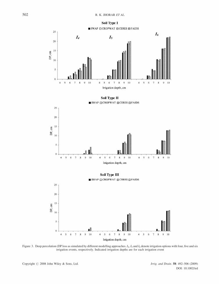
Figure 3. Deep percolation (DP loss as simulated by different modelling approaches. I4, I5 and I6 denote irrigation options with four, five and sixirrigation events, respectively. Indicated irrigation depths are for each irrigation event


DOI: 10.1002/ird


Figure 4. Scheduling index (Equation (2)) for different irrigation options. Irrigation depth corresponding to peak of curve is taken asrecommended depth


CERES(A) results in a specification of 9 cm as the recommended depth for irrigation option I4. Considering only

SWAP simulations, if the applied depth in irrigation option I6 is increased from 8 to 9 cm, deep percolation

increases from 5 to 8 cm, while relative transpiration increases from 0.79 to 0.82. On the other hand, if the

application depth is decreased from 8 to 6 cm, the resulting relative transpiration would be 0.67. Therefore, the


DOI: 10.1002/ird


recommendation resulting from CROPWAT(A) for irrigation option I4 has the risk of reduced crop production and

that of CERES(A) and FAIDS(A) has the risk of increased deep percolation loss when compared with SWAP.

Soil type II. According to the criteria of scheduling index, SWAP results in an optimum depth of application of

9, 7 and 7 cm for irrigation option I4, I5 and I6, respectively. The corresponding optimum depths resulting from

CROPWAT(A), FAIDS(A) and CERES(A) simulation are 8, 7 and 6 cm. The risk of deep percolation loss for the

recommended irrigation depths is very low for this soil type (Figure 3). Despite some differences in the

recommended irrigation application depths for I4 and I6, the expected yields may not be affected much. Considering

only SWAP simulations, when the depth of application is decreased from 9 to 8 cm for I4, the relative transpiration

decreases from 1.0 to 0.96. Decreasing irrigation application depth from 7 to 6 cm for I6 results in a relative

transpiration reduction from 1.0 to 0.95.

Soil type III. SWAP results in a specification of irrigation application depths of 9, 7 and 7 cm for I4, I5 and I6,

respectively. The corresponding optimum depths resulting from CROPWAT(A), FAIDS(A) and CERES(A)

simulation are 8, 6 and 6 cm. Again the risk of deep percolation loss for the recommended irrigation depths is very

low and expected yield is also not much affected due to differences in the recommended application depth.

CONCLUDING REMARKS

The basic purpose of this study was to check the reliability of different modelling approaches in the context of soil

water balance simulations. Therefore, the findings must not be interpreted to consider a particular model superior or

inferior in comparison to others as not all the options (e.g. interaction of environmental variables and agronomic

management vis-a-vis crop growth considered by CERES) of different models were exploited. Cumulative water

balance components have been compared to test different modelling approaches. Model predictions of water

balance components may be affected by the different approaches used for describing evapotranspiration (Clemente

et al., 1994). In this study the soil water balance subroutines of CROPWAT, CERES and FAIDS were reformulated

to incorporate a evapotranspiration process similar to that used in SWAP.

Different criteria have been proposed to interpret simulated water balance components in the form of practical

guidelines for efficient water management. In this paper, a new criterion is developed to evaluate irrigation

simulations under deep water table conditions and limited water availability. The developed scheduling index helps

in choosing an appropriate depth of application resulting in satisfactory evapotranspiration with minimum

percolation losses. Calculation of the index requires simple water balance components (actual total ET and

percolation losses) which are simulated by most irrigation simulation models.

Three of the four selected models use the concept of field capacity to determine the lower limit of drained water

below crop root zone. Typically, the moisture content at field capacity is related to 100, 300 and 500 cm soil

moisture tension in coarse, medium and fine-textured soils, respectively (Oswal, 1983). This means that at field

capacity the soil moisture tension is in increasing order for coarse, medium and fine-textured soils. The field

capacity, determined by calibration against SWAP-simulated water balance components for three soils studied in

the present study, shows a reverse trend. For example, the field capacity as calibrated for the CROPWAT approach

corresponds to soil moisture tension of 75, 60 and 55 cm for sandy loam, loam and sandy clay loam soil,

respectively. The different values of field capacity obtained for different models indicate the need to consider this a

calibration parameter rather than defining it at a particular pF. This implies that even the simple models like

CROPWAT, when used for irrigation planning, must be calibrated against observed water balance components.

The simulation results presented in this study show that cumulative actual evapotranspiration is reliably

predicted by different modelling approaches (when compared with SWAP) for normal to wet irrigation conditions.

However, the results obtained for shallow and less frequent irrigations indicate that the approach used in

CROPWATand CERES, and in FAIDS, may underestimate or overestimate actual evapotranspiration for relatively

dry conditions. The underestimation by the CROPWAT and CERES approaches is due to the neglect of possible


DOI: 10.1002/ird


upward flow from adjoining deeper wet layers. The over-predictions of actual evapotranspiration by the FAIDS

approach is attributed to the simplified principle followed to estimate upward flow.

Estimation of deep percolation loss associated with alternative irrigation options is an important consideration

for irrigation planning in arid and semi-arid regions. Comparison of predicted deep percolation for different

irrigation regimes revealed that, when compared with SWAP, the CERES approach outperformed the CROPWAT

and FAIDS approaches. As the risk of deep percolation increases (too wet conditions) all the models perform

equivalently.

Percolation loss is more sensitive to depth of application to lighter soil than on heavy soils. Therefore, it is

important to apply the precise optimal amount of irrigation for lighter soils (Burke et al., 1999). For a light soil

(sandy loam), all three modelling approaches resulted in a prescription of the same (6 cm) water application depth

for two of the three irrigation options simulated in this study. The models differed in the prescribed depth of

application for the irrigation option with less frequent irrigations. The differences in the recommended water

application depth for the other two soils (loam and sandy clay loam) were not large enough to cause any concern.

This means that, if properly calibrated, any of the modelling approaches may be used for irrigation planning.

The results presented in this paper are based on the cumulative water balance components. The findings of this

study are not valid for situations where temporal variations in fluxes are an important consideration. Also, the

presented results are for uniform soil hydraulic properties in the root zone. The effectiveness of different modelling

approaches for non-uniform soil hydraulic properties with depth need to be checked.

REFERENCES

Agarwal MC, Khanna SS. 1983. Efficient Soil and Water Management in Haryana. Haryana Agricultural University: Hisar, India.

BastiaanssenWGM. 1993.Unsaturated flowmodelling in a saline environment. Mission Report to the Indo-Dutch Operational Research Project.

Interne Mededeling 272. DLO, Winand Staring Centre, Wageningen, The Netherlands.

Black TA, GardnerWR, Thurtel GW. 1969. The prediction of evaporation, drainage, and soil water storage for a bare soil. Soil Science Society of

America Journal 33: 655–660.

Burke S, Mulligan M, Thornes JB. 1999. Optimal irrigation efficiency for maximum plant production and minimum water loss. Agricultural

Water Management 40: 372–381.

Clemente RS, de Jong R, Hayhoe HN, Raynolds WD, Hares M. 1994. Testing and comparison of three unsaturated soil water flow models.

Agricultural Water Management 25: 135–152.

Feddes RA, Kowalik PJ, Zarandy H. 1978. Simulation of field water use and crop yield. Simulation Monographs, Pudoc, Wageningen.

Feddes RA, Kabat P, van Bakel PJT, Bronswijk JJB, Halbertsma J. 1988. Modelling soil water dynamics in the unsaturated zone: sate of art.

Journal of Hydrology 100: 69–111.

Hillel D. 1980. Fundamentals of Soil Physics. Academic Press: San Diego, CA.

Kabat P, Feddes RA. 1995. Modelling soil water dynamics and crop water uptake at the field level. In Modelling and Parameterization of the

Soil–Plant–Atmosphere System, Kabat P, Marshall B, van den Broek BJ, Vos J, van Keulen J (eds). Wageningen Pers: Wageningen;

103–134.

Kabat P, Marshall B, van den Broek BJ, Vos J, van Keulen J (eds). 1995. Modelling and Parameterization of the Soil–Plant–Atmosphere

System. Wageningen Pers: Wageningen.

Oswal MC. 1983. A Textbook of Soil Physics. Vikas: New Delhi.

Ritchie JT. 1972. A model for predicting evaporation from a row crop with incomplete cover. Water Resources Research 8: 1204–1213.

Roest CWJ, Rijtema PE, Abdel Khalek MA, Boels D, Abdel Gawad ST, El Quosy DE. 1993. Formulation of the on-farm water management

model ’FAIDS’. Report 24: Reuse of Drainage Water Project. Drainage Research Institute, Quanter, Cairo.

Rubinstein RY. 1981. Simulation and the Monte Carlo Method. Wiley: New York.

Silberstein RP. 2006. Hydrological models are so good, do we still need data? Environmental Modelling and Software 21: 1340–1352.

Singh R, Singh J. 1997. Irrigation planning in wheat (Triticum aestivum) under deep water table conditions through simulation modelling.

Agricultural Water Management 33: 19–29.

Singh R, Jhorar RK, van Dam JC, Feddes RA. 2006. Distributed ecohydrological modeling to evaluate irrigation system performance in Sirsa

district, India. II: Impact of viable water management scenarios. Journal of Hydrology 329: 714–723.

Smith M. 1992. CROPWAT: a computer program for irrigation planning and management. Irrigation and Drainage Paper 46. FAO: Rome.

Smith M. 1996. Summary report, conclusions and recommendation of ICID/FAO workshop on Irrigation Scheduling, Rome, 12–13 September

1995. Water Report No. 8, FAO, Rome; 1–16.


DOI: 10.1002/ird


van Dam JC, Huygen J, Wesseling JG, Feddes RA, Kabat P, van Walsum PEV, Groenendijk P, van Diepen CA. 1997. Simulation of water flow,

solute transport and plant growth in the soil–water–atmosphere–plant environment: theory of SWAP version 2.0. Report No. 71, Department

of Water Resources, Wageningen Agricultural University, Netherlands.

van den Broek BJ (ed.). 1996. Dutch experience in irrigation water management modelling. Report No. 123, DLOWinand Starring Centre for

Integrated Land, Soil and Water Research, Wageningen, Netherlands.

van Genuchten MT. 1980. A closed form equation for predicting the hydraulic conductivity of unsaturated soils. Soil Science Society of America

Journal 44: 892–898.

Vogel T, HuangK, Zhang R, van GenuchtenMTh. 1996. TheHYDRUS code for simulating one-dimensional water flow, solute transport and heat

movement in variably saturated media. Research Report 140, US Salinity Laboratory, ARS-USDA, Riverside, CA.


DOI: 10.1002/ird

Documents

Effect of model selection on computed water balance components