Effect of individual observations on the Box–Cox transformation

Journal of Applied Statistics, 2013Vol. 40, No. 7, 1561–1571, http://dx.doi.org/10.1080/02664763.2013.789007

Effect of individual observations on theBox–Cox transformation

L.I. Pettit∗ and N. Sothinathan

School of Mathematical Sciences, Queen Mary University of London, London, E1 4NS, UK

(Received 11 June 2012; accepted 20 March 2013)

In this paper, we consider the influence of individual observations on inferences about the Box–Cox powertransformation parameter from a Bayesian point of view. We compare Bayesian diagnostic measures withthe ‘forward’ method of analysis due to Riani and Atkinson. In particular, we look at the effect of omittingobservations on the inference by comparing particular choices of transformation using the conditionalpredictive ordinate and the kd measure of Pettit and Young. We illustrate the methods using a designedexperiment. We show that a group of masked outliers can be detected using these single deletion diagnostics.Also, we show that Bayesian diagnostic measures are simpler to use to investigate the effect of observationson transformations than the forward search method.

Keywords: Bayesian methods; deletion diagnostics; influential observations; masking; outliers

1. Introduction

The main aim of this article is to analyse the influence of individual observations on the Box–Cox transformation from a Bayesian point of view and compare with the ‘forward’ method ofanalysis [13].

A number of authors have considered this problem from a classical point of view, oftenconcentrating on regression [1–4,6,8]. A Bayesian approach to this problem is given in [11].

A robust ‘forward search’ diagnostic method was proposed in [13] for the analysis of data.This used robust parameter estimates to reveal masked outliers in regression, using a forwardsearch procedure. The robust estimators used are least median of square for regression [14] andthe minimum volume ellipsoid for multivariate outliers [15]. In this article, the ordering fromthe forward search method has been used to provide information about transformations and forthe detection of outliers and influential observations in linear models. The forward search is usedon data subjected to various Box–Cox power transformations, as well as on untransformed data.Several forward plots are presented which can be used to assess the influence of the observations,possible outliers, the existence of masked outliers and also the adequacy of the transformations. Atypical output from the analysis is a plot of the score statistics for transformation as the number of

∗Corresponding author. Email: [email protected]

© 2013 Taylor & Francis

1562 L.I. Pettit and N. Sothinathan

observations used to fit the model is increased. This plot is called a ‘fan plot’, which is able to showthe influence of individual observations, not just outliers, on the evidence for a transformation.It is also shown that even if no outliers are present, the procedure provides an elegant graphicalsummary of the evidence for a transformation.

We consider this problem from a Bayesian point of view. We use well-known diagnostic mea-sures, namely the conditional predictive ordinate (CPO) [7,10] and kd [12] to search for outliersrelative to particular transformations and for observations which are influential on Bayes factorsin determining an appropriate transformation. We illustrate the methods using the poison datagiven in [5] and the modifications to it made in [13].

In Section 2, we define the Bayesian diagnostic measures we are going to use; the Bayes factor,kd and CPO. In Section 3, we reanalyse the poison data using these diagnostics and compare ourresults with those in [13].

2. Box–Cox transformations and Bayesian diagnostics

2.1 Box–Cox transformation

Consider the standard linear model

y = Xθ + ε, (1)

where y = (y1, y2, . . . , yn), θ = (θ0, θ1, . . . , θp−1) denotes a p × 1 vector of unknown coefficients,X = (xT

1 , xT2 , . . . , xT

n ) is an n × p design matrix with rank(X) = p and x1 a vector of ones and ε =(ε1, ε2, . . . , εn) represents the error term. The error terms εi are often assumed to be independentand identically distributed with a normal distribution, N(0, σ 2). Let θ̂ = (θ̂0, θ̂1, . . . , θ̂p−1) be anyestimate of parameter θ .

When the assumption of normality for the model equation (1) is not valid, [5] consider thefollowing transformation when y > 0.

y(λ) =⎧⎨⎩

yλ − 1

λλ �= 0,

log y λ = 0.(2)

The likelihood function relative to the transformed observations is

p(y | θ , σ , λ) = (2πσ 2)−n/2 exp

{− (y(λ) − Xθλ)

T(y(λ) − Xθλ)

2σ 2

}, (3)

so the likelihood function relative to the original untransformed observations is going to be

p(y | θ , σ , λ) = (2πσ 2)−n/2 exp

{−Sλ + (θ − θ̂λ)

TXTX(θ − θ̂λ)

2σ 2

}Jλ, (4)

where the Jacobian

Jλ =n∏1

yλ−1i ,

θ̂λ = (XTX)−1XTy(λ)

and

Sλ = (y(λ) − X θ̂λ)T(y(λ) − X θ̂λ).

Journal of Applied Statistics 1563

2.2 Bayes factor

We present the Bayes factor comparing two possible values of λ as in [11]. Using a non-informativeprior suggested in [9],

p(θ , σ , λ) ∝ p0(λ)

σ p+1,

it follows that the joint posterior is

p(θ , σ , λ | y) ∝ p(y | θ , σ , λ) × p(θ , σ , λ)

∝ σ−n−p−1 exp

{−Sλ + (θ − θ̂λ)

TXTX(θ − θ̂λ)

2σ 2

}Jλp0(λ).

In [9] it is assumed p0(λ) is uniform over the region of λ’s under consideration,

p0(λ) = c,

where c is a constant. To obtain the posterior of λ, we integrate the above joint posterior withrespect to θ and σ ,

p(λ | y) ∝∫ ∫

σ−n−p−1 exp

{−Sλ + (θ − θ̂λ)

TXTX(θ − θ̂λ)

2σ 2

}Jλp0(λ) dθ dσ .

It follows that

p(λ | y) ∝ Jλ(Sλ)−n/2,

so the Bayes factor comparing the choice of two particular choices of λ0 and λ1 is

B01 = p(λ0 | y)

p(λ1 | y)

= Jλ0

Jλ1

{Sλ0

Sλ1

}−n/2

.

2.3 Condtional predictive ordinate

The CPO measures how surprising observation d is. It is defined as

CPO = p(yd | y(d)), (5)

where y(d) is the data omitting the dth observation. Small values of Equation (5) indicate thatyd is surprising in the light of prior knowledge and the other observations. For the particulartransformation λ, the CPO can also be written in the following way

CPO(λ) = p(y|λ)

p(y(d)|λ).

Using standard integration, we find that

p(y | λ) = 2n/2−1 Jλ(2π)−(n−p)/2

|XTX|1/2�

(n

2

)(Sλ)

−n/2.


Similarly

p(y(d)|λ) = 2(n−3)/2 J(d)λ(2π)−(n−p−1)/2

|XT(d)X(d)|1/2

�

(n − 1

2

)(S(d)λ)

−(n−1)/2.

It follows that

CPO(λ) = (π)−(1/2)yλ−1d

�(n/2)

�((n − 1)/2)

|XT(d)X(d)|1/2

|XTX|1/2

[S(d)λ](n−1/2)

[Sλ]n/2.

2.4 The effect of observations on the Bayes factor

In [12] the diagnostic measure kd is introduced to measure the effect on a Bayes factor ofobservation d. The quantity kd is defined as follows.

kd = log10 B01 − log10 B(d)01 ,

where B(d)01 is the Bayes factor excluding observation d. If the value of kd is large, then the

observation d has a large influence on the Bayes factor. Suppose that we are interested in comparingmodel M0 with model M1 using a Bayes factor. If kd < 0, there is an increase of evidence forM0 when observation d is deleted, that is observation d itself favours model M1. Similarly, whenkd > 0 observation d favours model M0. The sign of kd (i.e. whether < 0 or > 0) is not enough tochange our beliefs whether deletion of observation d is supporting M0 to supporting M1. log B(d)

01can be plotted against d to see whether deleting observation d changes our beliefs.

First we need to decide what order to exclude observations. There is a possibility to excludethe observation with maximum value of |kd | and then to condition on excluding this. Thus, thesequence would be

kd = log B01 − log B(d)01 ,

kde = log B(d)01 − log B(de)

01

and so on. We can also write kd in a different way. If we substitute

B01 = p(y | M0)

p(y | M1)

then we get

kd = logp(y | M0)

p(y | M1)− log

p(y(d) | M0)

p(y(d) | M1).

So that kd is the difference in the logarithms of the CPO for the two models M0 and M1. That is

kd = log10

(CPOM0

CPOM1

)

= log10

[yλ0−λ1

d

(Sλ0(d)

Sλ1(d)

)(n−1)/2 (Sλ1

Sλ0

)n/2]

= (λ0 − λ1) log10 yd + n − 1

2log10

[RSSλ0(d)

RSSλ1(d)

]− n

2log10

[RSSλ0

RSSλ1

],

where RSS is the residual sum of squares and RSS(d) the residual sum of squares after deletingobservation d.

In [12] it is suggested that if |kd | > 0.5 then the observation d might be thought of as influential.


3. Application to the poison data

3.1 Riani and Atkinson’s analysis

We consider the poison data which was originally analysed in [5]. Table 1 shows the originalpoison data – survival times of 48 animals exposed to three different poisons and subject to fourdifferent treatments. The experiment was set out in a 3 × 4 factorial design with a replication of4. It is assumed that there is no interaction and if possible, the aim to find a transformation forwhich an additive model is appropriate, the cell variances are equal and the errors are normallydistributed.

This example is discussed in [13] to illustrates the behaviour of their procedure for the trans-formation of the response. Their analysis is based on five values of the transformation λ whichare −1 (inverse), −0.5 (inverse square root), 0 (log), 0.5 (square root), 1.0 (no transformation).

During their whole forward search, there is no evidence against either λ = −1 (i.e. reciprocaltransformation) or λ = −0.5 (i.e. inverse square root transformation). The log transformation isalso acceptable until the last four observations are included by the forward search. Table 2 givesthe last six observations to enter in each transformation.

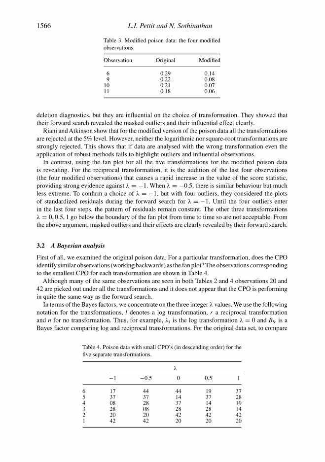
Riani and Atkinson were interested in how multiple masked outliers can indicate an incorrecttransformation. To generate masked outliers, they made four small observations even smalleras shown in Table 3. They suggested that these masked outliers cannot be detected by single

Table 1. Box and Cox poison data – survival times of 48 animalsexposed to three different poisons and subject to four differenttreatments.

Treatments

Poison A B C D

1 0.31 0.82 0.43 0.450.45 1.10 0.45 0.710.46 0.88 0.63 0.660.43 0.72 0.76 0.62

2 0.36 0.92 0.44 0.560.29 0.61 0.35 1.020.40 0.49 0.31 0.710.23 1.24 0.40 0.38

3 0.22 0.30 0.23 0.300.21 0.37 0.25 0.360.18 0.38 0.24 0.310.23 0.29 0.22 0.33

Table 2. For poison data, last six observations to enter the five separatetransformations using the forward search.

λ

m −1 −0.5 0 0.5 1

43 27 44 14 43 2844 28 37 28 28 4345 37 28 37 14 1746 44 08 17 17 1447 11 20 20 42 4248 08 42 42 20 20


Table 3. Modified poison data: the four modifiedobservations.

Observation Original Modified

6 0.29 0.149 0.22 0.08

10 0.21 0.0711 0.18 0.06

deletion diagnostics, but they are influential on the choice of transformation. They showed thattheir forward search revealed the masked outliers and their influential effect clearly.

Riani and Atkinson show that for the modified version of the poison data all the transformationsare rejected at the 5% level. However, neither the logarithmic nor square-root transformations arestrongly rejected. This shows that if data are analysed with the wrong transformation even theapplication of robust methods fails to highlight outliers and influential observations.

In contrast, using the fan plot for all the five transformations for the modified poison datais revealing. For the reciprocal transformation, it is the addition of the last four observations(the four modified observations) that causes a rapid increase in the value of the score statistic,providing strong evidence against λ = −1. When λ = −0.5, there is similar behaviour but muchless extreme. To confirm a choice of λ = −1, but with four outliers, they considered the plotsof standardized residuals during the forward search for λ = −1. Until the four outliers enterin the last four steps, the pattern of residuals remain constant. The other three transformationsλ = 0, 0.5, 1 go below the boundary of the fan plot from time to time so are not acceptable. Fromthe above argument, masked outliers and their effects are clearly revealed by their forward search.

3.2 A Bayesian analysis

First of all, we examined the original poison data. For a particular transformation, does the CPOidentify similar observations (working backwards) as the fan plot? The observations correspondingto the smallest CPO for each transformation are shown in Table 4.

Although many of the same observations are seen in both Tables 2 and 4 observations 20 and42 are picked out under all the transformations and it does not appear that the CPO is performingin quite the same way as the forward search.

In terms of the Bayes factors, we concentrate on the three integer λ values. We use the followingnotation for the transformations, l denotes a log transformation, r a reciprocal transformationand n for no transformation. Thus, for example, λl is the log transformation λ = 0 and Blr is aBayes factor comparing log and reciprocal transformations. For the original data set, to compare

Table 4. Poison data with small CPO’s (in descending order) for thefive separate transformations.

λ

−1 −0.5 0 0.5 1

6 17 44 44 19 375 37 37 14 37 284 08 28 37 14 193 28 08 28 28 142 20 20 42 42 421 42 42 20 20 20


Table 5. Values of kd for the poison data log versus reciprocaltransformation.

Treatments

Poison A B C D

1 −0.27 0.27 −0.12 −0.010.19 −0.01 −0.07 0.170.24 0.26 0.19 0.170.10 0.21 0.08 0.15

2 0.04 0.07 0.07 0.07−0.26 0.05 −0.21 −0.73

0.32 −0.27 −0.16 0.100.60 −0.87 −0.08 −0.13

3 −0.42 −0.41 −0.26 −0.22−0.40 0.01 −0.29 0.15

0.45 0.09 −0.31 −0.18−0.37 −0.42 −0.14 −0.07

λl = 0 versus λr = −1, we have log10 Blr = −2.49 which gives strong support that the appropriatetransformation is a reciprocal. The other pairwise Bayes factors log10 Bnl = −9.49 and log10 Bnr =−11.98 showing very clearly that a transformation is necessary.1

Table 5 gives the values of kd for the Bayes factor comparing the reciprocal and logarithmictransformations. As we would expect omitting the largest values gives a negative value of kd andthe smallest gives positive values of kd . We may suspect the observations 20 (poison 2, treatmentB and replicate 4), 8 (poison 2, treatment A and replicate 4) and 42 (poison 2, treatment D andreplicate 4) may be influencing our choice of transformation since these have the larger valuesof |kd |.

We now look at the effect of the modified data on the Bayes factors. We now have clearevidence against the reciprocal transformation. The pairwise Bayes factors are log10 Bnr = 15.86,log10 Bnl = −4.38 and log10 Blr = 20.24. Overall the logarithmic transformation is now preferred.

We now see whether we can detect the effect of the modified observations using our Bayesiandiagnostics. First we look at the values of kd . We consider the effect on the comparison of thereciprocal and logarithmic transformations since these are best supported for the original data.

Table 6 gives the values of kd for the modified poison data. It is clear that observation 11 ishighly influential because the value of k11 is large at 2.99.

We try omitting the 11th observation and recalculate kd for the remaining observations. Table 7gives the kd values without observation 11. We now see that observation 10 has a large value ofkd at 4.06. We now omit observation 10 as well and recalculate the values of kd . We see in Table 8that observation 9 now has a very large value of kd at 8.95. In Table 9, we see the values of kd

when we omit observations 9, 10 and 11. Now observation 6, the last of the modified values, hasa kd of 6.13. Sequential use of kd picks out all the four modified observations.

We see what happens after we delete observation 6. Table 10 gives the values of kd after deletingall four modified values. Now observation 8 has the largest value of kd . Other observations withlarge values of |kd | are 12, 20 and 42. Recall that observations 8, 20 and 42 were influentialin the original data set. Also observation 12 is now the only observation left for that particularpoison/treatment combination so is likely to be influential.

In a similar manner, we can look at the effect of the modified observations as measured by theCPO for different transformations. We see in Table 11 that the four modified observations are thefour most outlying observations for the reciprocal and square root reciprocal and all four are inthe smallest six for the logarithm and square root.


Table 6. Values of kd for the modified poison data log versusreciprocal transformation.

Treatments

Poison A B C D

1 0.44 0.47 0.36 −0.050.55 0.79 0.42 0.710.53 0.81 0.57 0.650.57 0.61 0.42 0.58

2 0.48 0.63 0.47 0.58−0.83 0.57 0.29 0.03

0.39 0.19 0.09 0.590.22 0.12 0.42 −0.01

3 0.23 0.30 0.20 0.360.97 0.49 0.21 0.392.99 0.51 0.21 0.380.10 0.25 0.19 0.39

Table 7. Values of kd for the modified poison data (without theobservation 11) log versus reciprocal transformation.

Treatments

Poison A B C D

1 0.29 0.69 0.29 −0.130.50 0.67 0.35 0.630.49 0.73 0.49 0.590.52 0.54 0.28 0.52

2 0.44 0.51 0.40 0.50−0.93 0.49 0.22 −0.18

0.38 0.11 0.03 0.490.07 −0.10 0.35 −0.09

3 1.62 0.17 0.12 0.284.06 0.42 0.14 0.32– 0.29 0.43 0.29

0.06 0.11 0.10 0.31

Table 8. Values of kd for the modified poison data (without observations10 and 11) log versus reciprocal transformation.

Treatments

Poison A B C D

1 0.10 0.59 0.19 −0.200.41 0.53 0.25 0.530.41 0.63 0.36 0.490.42 0.46 0.13 0.43

2 0.37 0.38 0.34 0.41−0.57 0.39 0.12 −0.42

0.36 0.01 −0.06 0.37−0.12 −0.35 0.27 −0.18

3 8.95 0.01 0.02 0.16– 0.42 0.04 0.23– 0.29 0.03 0.18

−0.07 −0.05 0.00 0.21


Table 9. Values of kd for the modified poison data (without observations9, 10 and 11) log versus reciprocal transformation.

Treatments

Poison A B C D

1 −0.17 0.39 −0.00 −0.220.23 0.26 0.05 0.310.24 0.41 0.19 0.290.19 0.28 0.01 0.24

2 0.23 0.22 0.18 0.216.13 0.19 −0.09 −0.540.36 −0.19 −0.24 0.22

−0.21 −0.56 0.08 −0.313 – 0.22 −0.14 −0.08

– 0.05 −0.18 0.04– 0.08 −0.17 −0.06

−0.41 −0.25 −0.09 −0.02

Table 10. Values of kd for the modified poison data (without observa-tions 6, 9, 10 and 11) log versus reciprocal transformation.

Treatments

Poison A B C D

1 −0.07 0.24 −0.09 −0.040.07 0.00 0.26 0.150.11 0.24 0.22 0.140.01 0.17 0.07 0.11

2 −0.07 0.13 −0.24 0.04– 0.01 −0.19 −0.55

0.14 −0.31 −0.09 0.141.29 −0.69 −0.25 −0.15

3 – −0.34 −0.34 −0.22– 0.04 −0.32 0.07– −0.32 −0.09 −0.20

−0.55 −0.15 −0.08 −0.11

Table 11. Modified poison data with small CPO’s (in descendingorder) for the five separate transformations.

λ

−1 −0.5 0 0.5 1

6 42 20 11 11 145 20 42 42 6 64 11 11 20 42 103 10 10 6 10 422 9 9 10 20 91 6 6 9 9 20


4. Discussion

In [13] a method is presented for detecting which observations are influential in choosing atransformation. By considering the poison data modified to include four masked outliers, theyshow that their method can cope with such contamination. In this paper, we have shown that byusing two Bayesian single deletion diagnostics, we have also been able to identify the maskedoutliers. The advantage of the Bayesian diagnostics is that they do not require nearly as muchcomputing power as the forward search method.

It has been pointed out by a referee that the results are based on a particular choice of priordistribution. How sensitive are they to this choice? To examine this question, we considered theprior originally suggested in [5]. This was, in the notation of this paper,

p0(λ) ∝ 1

σ

1

Jp/nλ

.

It follows that the joint posterior is

p(θ , σ , λ | y) ∝ p(y | θ , σ , λ) × p(θ , σ , λ)

∝ σ−n−1 exp

{−Sλ + (θ − θ̂λ)

TXTX(θ − θ̂λ)

2σ 2

}J(n−p)/nλ .

To obtain the posterior of λ we integrate the above joint posterior with respect to θ and σ ,

p(λ | y) ∝∫ ∫

σ−n−p−1 exp

{−Sλ + (θ − θ̂λ)

TXTX(θ − θ̂λ)

2σ 2

}J(n−p)/nλ dθ dσ .

It follows that

p(λ | y) ∝ J(n−p)/nλ (Sλ)

−(n−p)/2,

so the Bayes factor comparing the choice of two particular choices of λ0 and λ1 is

B01 = p(λ0 | y)

p(λ1 | y)

= Jλ0

Jλ1

(n−p)/n {Sλ0

Sλ1

}−(n−p)/2

={

Jλ0

Jλ1

{Sλ0

Sλ1

}−n/2}(n−p)/n

.

Thus the Bayes factor using the prior in [5] is the Bayes factor based on the prior in [9] raised tothe power (n − p)/n. Note that this means that although the value of kd would be slightly smaller,the ordering would be unchanged.

Note

1. Code, written for S-plus, to calculate the Bayes factors and values of kd are available from the authors.

References

[1] A.C. Atkinson, Regression and transformations and constructed variables (with discussion), J. Roy. Statist. Soc. B44 (1982), pp. 1–36.


[2] A.C. Atkinson, Plots, Transformations and Regression, Oxford University Press, Oxford, 1985.[3] A.C. Atkinson, Diagnostic tests for transformations, Technometrics 28 (1986), pp. 29–37.[4] A.C. Atkinson, Robust regression and unmasking transformations, in Proceedings of the Second International

Tampere Conference in Statistics, T. Pukkila and S. Puntanen, eds., University of Tampere, Finland, 1987, pp. 99–112.[5] G.E.P. Box and D.R. Cox, An analysis of Transformations (with discussion), J. Roy. Statist. Soc. B 26 (1964),

pp. 211–246.[6] R.D. Cook and P.C. Wang, Transformations and influential cases in regression, Technometrics 25 (1983),

pp. 337–343.[7] S. Geisser, Discussion of sampling and Bayes’ inference in scientific modelling and robustness (by G.E.P. Box),

J. Roy. Statist. Soc. 143 (1980), pp. 416–417.[8] D.V. Hinkley and S. Wang, More about transformations and influential cases in regression, Technometrics 30 (1988),

pp. 435–440.[9] L.R. Pericchi, A Bayesian approach to transformations to normality, Biometrika 68 (1981), pp. 35–43.

[10] L.I. Pettit, The conditional predictive ordinate for the normal distribution, J. Roy. Statist. Soc. B 52 (1990),pp. 175–184.

[11] L.I. Pettit, Bayes factors and the effect of individual observations on the Box–Cox transformation, in BayesianStatistics 4, J.M. Bernardo, J.O. Berger, A.P. Dawid, and A.F.M. Smith, eds., Oxford University Press, Oxford, 1992,pp. 731–739.

[12] L.I. Pettit and K.D.S. Young, Measuring the effect of observations on Bayes factors, Biometrika 77 (1990),pp. 455–466.

[13] M. Riani and A.C. Atkinson, Robust diagnostic data analysis: Transformation in regression, Technometrics 42(2000), pp. 384–394.

[14] P.J. Rousseeuw, Least median of squares regression, J. Amer. Statist. Assoc. 79 (1984), pp. 871–880.[15] P.J. Rousseeuw and B.C. Van Zomeren, Unmasking multivariate outliers and leverage points, J. Amer. Statist. Assoc.

85 (1990), pp. 633–639.

Documents

Effect of individual observations on the Box–Cox transformation