Embed Size (px)
Citation preview

Effect of Ambient Pressure on Diesel Spray AxialVelocity and Internal
Structure
Alan Kastengren, Christopher Powell Center for Transportation Research
Argonne National Laboratory
Kyoung-Su Im, Yujie Wang, and Jin Wang Advanced Photon Source
Argonne National Laboratory
DOE FreedomCAR & Vehicle TechnologiesProgram
Program Manager: Gupreet Singh

Good Understanding of Spray Structure isImportant in Diesel Combustion
�Performance and emissions of diesel engines are closely tied to the spray from the injector – Excessive penetration → wall wetting → UHC emissions – Poor spray pattern → poor fuel-air mixing → increased
emissions �Two of the most important variables that effect spray
behavior are injection pressure and ambient density– Penetration speed increased by higher injection pressure
and lower ambient density – Cone angle seems to increase as ambient density
increases
2

Current Spray Diagnostic Techniques AreInadequate
�Most spray measurements are based on optical measurements – Adequate for measuring penetration speed – Can’t probe internal spray structure in dense regions – Often not quantitative, due to strong scattering effects
�There are important parameters these optical techniques can’t show – Mass distribution of fuel in the spray – Fuel velocity away from the leading edge
�Need a nonintrusive, quantitative technique to measure sprays
3

X-Rays Give a Quantitative Determination ofFuel Distribution
N2 FlowX-Ray
Window
Fuel Injector
8 KeV X-ray Beam
I I0 Avalanche Photodiode
X-Y Slits 30 μm (V)
x200 μm (H)
I0 Incident x-ray intensity I = I e−MμM0
I Measured x-ray intensity μM Fuel absorption coefficient M = ln(I0 / I ) M Projected mass density, mass/area μM
4

Radiography Has Good Spatial and TimeResolution
�Resulting data: 2-D fuel mass distribution as a function of time �Measurement range
– 0.2 – 6.0 mm axial – -1.4 – 1.2 mm transverse – 2 ms of data
�Time step 3.68 μs – 0.07 CAD at 3000 rpm
Measurement Grid
5

Experiment Details
� Light-duty diesel common-rail injector: solenoid driven
� Axial single hole – Non-hydroground: r/D = 0.2 – Orifice diameter 207 μm – L/D = 4.7
� Injection parameters – Injection pressure: 500 and 1000 bar – Injection duration: 1000 μs – Ambient gas: N2 at room temperature – Ambient pressure: 5 bar and 20 bar – Liquid: Diesel calibration fluid with
cerium additive
6
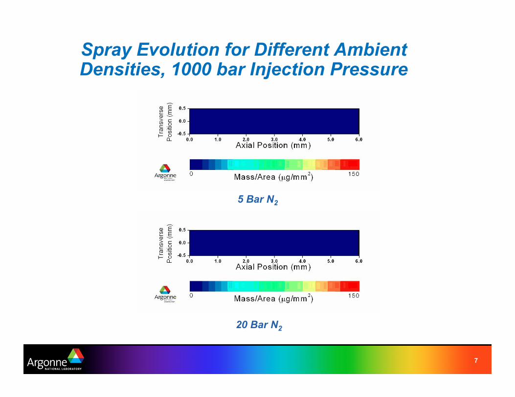
Spray Evolution for Different AmbientDensities, 1000 bar Injection Pressure
5 Bar N2
20 Bar N2
7

Spray Evolution for Different InjectionPressures, 5 Bar Ambient N2
500 bar
1000 bar
8

Penetration Results
�Penetration of leading edge vs. time � Increased ambient density
reduces penetration speed – Not as much as accepted
correlations indicate
� Lower injection pressure reduces penetration speed – More than expected
�Dynamics of injector opening are important to early penetration results Penetration
9

Previous Cone Angle Results
�Cone angle measurements help explain how the fuel mixes with the ambient gas �Typically found by examining optical spray images �X-ray radiography gives much more detail than optical
measurements on the internal mass distribution – Based on a well-defined, quantitative measure of the fuel
distribution – Can record cone angle as a function of time
10

Snapshot 100, 1000 bar, 5 bar
Use of Radiography to Find Cone Angle
11

Cone Angle Changes Significantly with Time
� Define cone angle based on the mass distributions across the spray
� Time period of few hundred µs for cone angle to reach steady state
� Much smaller than typical optical cone angles – Examining spray core – Optical measurements show
spray periphery � Injection pressure has little
effect on steady state cone angle
� Increased chamber pressure increases cone angle
12

Spray Axial Velocity Determination
�Axial velocity of spray in dense regions of the spray is not well known �Axial velocity affects:
– Penetration speed – Shear with ambient gas – Initialize spray breakup models
�Radiography can be used to determine the mass-averaged axial velocity of the spray for limited time spans near the beginning of the spray event – Due to quantitative measurement of mass as a function of time – Velocity measured as a function of both x and t – Limited to time just after the start of injection
13
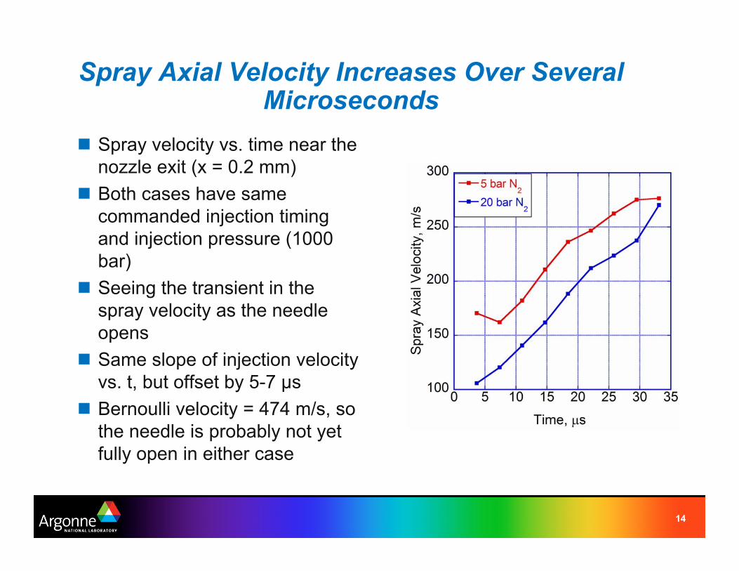
Spray Axial Velocity Increases Over SeveralMicroseconds
� Spray velocity vs. time near the nozzle exit (x = 0.2 mm)
� Both cases have same commanded injection timing and injection pressure (1000 bar)
� Seeing the transient in the spray velocity as the needle opens
� Same slope of injection velocity vs. t, but offset by 5-7 µs
� Bernoulli velocity = 474 m/s, so the needle is probably not yet fully open in either case
14

Spray Axial Velocity Is Strongly Affected byAmbient Density
� Spray velocity vs. x 33 µs after SOI
� Spray moves more slowly as distance from nozzle increases – Reduction in spray velocity due
to aerodynamic interactions
– Fluid at spray tip was injected at a slower velocity and so should move more slowly
� Difference in the two curves suggests that aerodynamic interactions slow the spray down more quickly with axial distance at higher ambient density
15

Future Work
�Continue to increase ambient pressure (density) of measurements – Further measurements at 30 bar ambient pressure in the near
future – Near the ambient density in-cylinder near TDC
�Perform measurements on multi-hole nozzles – More representative of applied nozzle geometries – More parameters to explore: spray angle, VCO vs. minisac
�Further refine the velocity determination – Improve signal/noise of measurements – Attempt to incorporate mechanical ROI measurements with the x-
ray density measurements
16
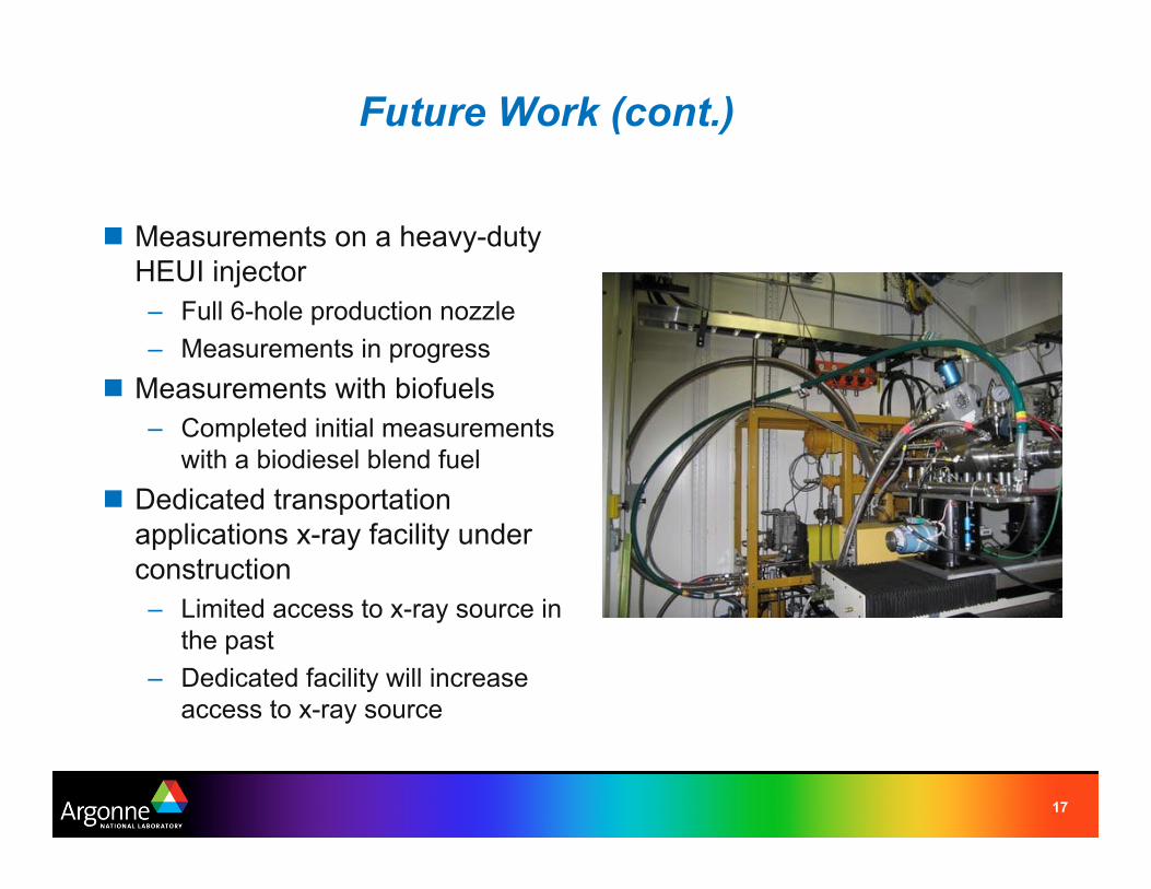
Future Work (cont.)
� Measurements on a heavy-duty HEUI injector – Full 6-hole production nozzle – Measurements in progress
� Measurements with biofuels – Completed initial measurements
with a biodiesel blend fuel � Dedicated transportation
applications x-ray facility under construction – Limited access to x-ray source in
the past – Dedicated facility will increase
access to x-ray source
17

),(),(),(
0
00 txTIM
txxmtxV cvma
>=&
Future Work: Spray Axial Velocity y Determination
Control Volume xz
Injector
Spray
x=x0
∞ ∞∞ ∞ m& cv (x > x0 , t) = − ∫ ∫ ρ(x0 , y, z, t) ⋅V (x0 , y, z, t) • n̂ ⋅ dz ⋅ dy ∫ ∫ ρ(x0, y, z, t) ⋅Vx (x0, y, z, t) ⋅ dz ⋅ dy
−∞ −∞ Vma (x0, t) = −∞ −∞ ∞ ∞ ∞ ⎡ ∞ ⎤
= ρ(x0 , y, z, t) ⋅Vx (x0 , y, z, t) ⋅ dz ⋅ dy ⎢ ρ(x0, y, z, t) ⋅ dz⎥ ⋅ dy∫ ∫ ∫ ∫⎢ ⎥−∞ −∞ −∞ ⎣−∞ ⎦
18