DOT/FAA/AR-03/65 Office of Aviation Research Washington, D.C. 20591

Effect of Airfoil Geometry on Performance With Simulated Ice Accretions Volume 2: Numerical Investigation August 2003 Final Report This document is available to the U.S. public through the National Technical Information Service (NTIS), Springfield, Virginia 22161.

U.S. Department of Transportation Federal Aviation Administration

NOTICE

This document is disseminated under the sponsorship of the U.S. Department of Transportation in the interest of information exchange. The United States Government assumes no liability for the contents or use thereof. The United States Government does not endorse products or manufacturers. Trade or manufacturer's names appear herein solely because they are considered essential to the objective of this report. This document does not constitute FAA certification policy. Consult your local FAA aircraft certification office as to its use. This report is available at the Federal Aviation Administration William J. Hughes Technical Center's Full-Text Technical Reports page: actlibrary.tc.faa.gov in Adobe Acrobat portable document format (PDF).

Technical Report Documentation Page 1. Report No. DOT/FAA/AR-03/65

2. Government Accession No. 3. Recipient's Catalog No.

4. Title and Subtitle

EFFECT OF AIRFOIL GEOMETRY ON PERFORMANCE WITH SIMULATED 5. Report Date

August 2003 ICE ACCRETIONS, VOLUME 2: NUMERICAL INVESTIGATION 6. Performing Organization Code

7. Author(s)

Jianping Pan and Eric Loth 8. Performing Organization Report No.

9. Performing Organization Name and Address

University of Illinois at Urbana-Champaign 10. Work Unit No. (TRAIS)

104 S. Wright Street Urbana, IL 61801

11. Contract or Grant No.

DTFAMB 96-6-023 12. Sponsoring Agency Name and Address

U.S. Department of Transportation Federal Aviation Administration

13. Type of Report and Period Covered

Final Report

Office of Aviation Research Washington, DC 20591

14. Sponsoring Agency Code

AIR-100 15. Supplementary Notes

The FAA William J. Hughes Technical Center Technical Monitor was James Riley. 16. Abstract

A computational study was completed in parallel with the experimental study to investigate the level of robustness of numerical methodologies for iced airfoil aerodynamic performance for a range of Reynolds and Mach numbers and to examine the effects of airfoil shape as well as ice shape location and height. The primary computational methodology employed herein was the WIND code. The grid sensitivity, turbulence model effect, and three-dimensional (3-D) capability aspects of WIND were assessed though detailed validations of selected clean and iced airfoil/wing cases. Of the various Reynolds-Averaged Navier-Stokes (RANS) turbulence models considered, the Mentor Shear Stress Transport and especially the Spalart-Allmaras models gave the best overall performance, and the latter was chosen for all the performance simulations. The WIND methodology was able to consistently predict the subtle measured trends associated with Reynolds and Mach numbers as well as the dramatic measured trends noted for variation in ice shape height and location, especially for upper surface ice locations and thick airfoils. For a leading-edge iced airfoil, the size effect is still significant but not as large and, in general, the variations in lift, drag, and pitching moment tend to vary more linearly with ice shape size. However, a significant shortcoming of the numerical methodology was the inability to predict a maximum lift coefficient (though such a maximum was noted in the experiments) for airfoils with a large upper surface ice shape; this result was consistent with other codes that use RANS turbulence models. To improve the predictive performance for iced airfoil aerodynamics with respect to stall conditions, unsteady 3-D numerical methodologies, which capture the vertical dynamics (such as Detached Eddy Simulations or Large Eddy Simulations), should be considered. 17. Key Words

Simulated ice shape, Computational fluid dynamics, Reynolds-Averaged Navier-Stokes, Turbulence model, Iced airfoil performance degradation

18. Distribution Statement

This document is available to the public through the National Technical Information Service (NTIS) Springfield, Virginia 22161.

19. Security Classif. (of this report)

Unclassified

20. Security Classif. (of this page)

Unclassified

21. No. of Pages

81 22. Price

Form DOT F1700.7 (8-72) Reproduction of completed page authorized

TABLE OF CONTENT

Page

EXECUTIVE SUMMARY

1. INTRODUCTION

2. PREVIOUS NUMERICAL STUDIES

2.1 Iced Airfoil RANS Simulations 2.2 Iced Wing RANS Simulations

3. COMPUTATIONAL METHODOLOGY

3.1 Navier-Stokes Equations 3.2 Simulation Programs

3.2.1 Overview of WIND 3.2.2 Overview of FLUENT

3.3 Turbulence Models and Transition

xi

1

2

2 4

5

5 6

6 7

7

3.3.1 Spalart-Allmaras Turbulence Model 8 3.3.2 Other Turbulence Models 9 3.3.3 Transition Point Specification 11

3.4 Grid Generation and Boundary Conditions 11

4. RESULTS AND DISCUSSION 13

4.1 Assesment of Numerical Parameters 13

4.1.1 Grid Dependence Sensitivity for Clean NACA 23012 Airfoil 13 4.1.2 Turbulence Model Sensitivity and Selection 17 4.1.3 Assessment for Clean and Iced Wings 19 4.1.4 Assessment of WIND vs FLUENT 23

4.2 Effect of Reynolds Number for NACA 23012 Airfoil 26

4.2.1 Effect of Reynolds Number for Clean Airfoil 26 4.2.2 Effect of Reynolds Number for Upper Surface Iced Airfoil 29

4.3 Effect of Mach Number for NACA 23012 Airfoil 34

4.3.1 Effect of Mach Number for Clean Airfoil 35 4.3.2 Effect of Mach Number for Upper Surface Iced Airfoil 37

iii

4.4 Effect of Ice Shape Size for Airfoils 39

4.4.1 Upper Surface Ice Shape Size Effect for NACA 23012 39 4.4.2 Leading-Edge Ice Shape Size Effect for NLF 0414 41

4.5 Effect of Wing vs Airfoil 43

5. CRITICAL ICE SHAPE METHODOLOGY 45

5.1 Effect of Ice Shape Location for Iced NACA 23012 Airfoil 45 5.2 Effect of Ice Shape Location on Other Airfoils 53 5.3 Effect of Ice Shape Location on Iced NACA 23012 Wing 62

6. SUMMARY, CONCLUSIONS, AND RECOMMENDATIONS 64

6.1 Summary 6.2 Conclusions 6.3 Recommendations

7. REFERENCES

LIST OF FIGURES

Figure

Typical Ice Accretion Shapes

64 65 67

67

Page

1

2 Lift Coefficient for a NACA 23012m Airfoil With k/c = 0.0083 Quarter-Round Ice Shape Located at x/c = 0.1 3

3 Drag Coefficient for a NACA 23012m Airfoil With k/c = 0.0083 Quarter-Round Ice Shape Located at x/c = 0.1 4

4 Typical Grid for an Iced NACA 23012 Airfoil 12

5 Lift Coefficient for a Clean NACA 23012 Airfoil at Re = 10.5x106 , M = 0.12 14

6 Drag Coefficient for a Clean NACA 23012 Airfoil at Re = 10.5x106 , M = 0.12 15

7 Pitching-Moment Coefficient for a Clean NACA 23012 Airfoil at Re = 10.5x106 , M = 0.12 16

8 Pressure Distribution for a Clean NACA 23012 Airfoil at Re = 10.5x106 , M = 0.12, α = 15° 17

iv

1

9 Lift Coefficient for an Iced NACA 23012 Airfoil at Re = 10.5x106, M = 0.12 18

10 Drag Coefficient for an Iced NACA 23012 Airfoil at Re = 10.5x106, M = 0.12 18

11 Pitching-Moment Coefficient for an Iced NACA 23012 Airfoil at Re = 10.5x106,M = 0.12 19

12 Three-Dimensional Grid for a Rectangular Clean NACA 0012 Wing 20

13 Sectional Lift Along the Span for a Clean NACA 0012 Wing at Re = 10.5x106,M = 0.15, α = 8° 20

14 Pressure Distribution for the Midspan of a Clean NACA 0012 Wing at Re = 10.5x106, M = 0.15, α = 8° 21

15 Sectional Lift Along the Span for an Iced NACA 0012 Wing at Re = 10.5x106,M = 0.15, α = 4° (8°) 21

16 Pressure Distribution for the Midspan of an Iced NACA 0012 Wing at Re = 10.5x106, M = 0.15, α = 4° 22

17 Pressure Distribution for the Midspan of an Iced NACA 0012 Wing at Re = 10.5x106, M = 0.15, α = 8° 22

18 Pressure Distribution for a Clean NACA 23012 Airfoil at Re = 10.5x106,M = 0.12, α = 0° With Second-Order Schemes 23

19 Pressure Distribution for a Clean NACA 23012 Airfoil at Re = 10.5x106,M = 0.12, α = 10° With Second-Order Schemes 24

20 Pressure Distribution for an Iced NACA 23012 Airfoil (k/c = 1.39%, x/c = 0.10) at Re = 10.5x106, M = 0.12, α = 0° for First-Order Schemes 25

21 Pressure Distribution for an Iced NACA 23012 Airfoil (k/c = 1.39%, x/c = 0.10) at Re = 10.5x106, M = 0.12, α = 0° With Second-Order Schemes 25

22 Reynolds Number Effect on Lift Coefficient for a Clean NACA 23012 Airfoil atM = 0.12 26

23 Reynolds Number Effect on Drag Coefficient for a Clean NACA 23012 Airfoil atM = 0.12 27

24 Reynolds Number Effect on Pitching-Moment Coefficient for a Clean NACA 23012 Airfoil at M = 0.12 27

25 Pressure Distributions for a Clean NACA 23012 Airfoil at Re = 10.5x106,M = 0.12 28

v

26 Reynolds Number Effect on Lift Coefficient for an Iced NACA 23012 Airfoil (k/c = 1.39%, x/c = 0.10) at M = 0.12 29

27 Lift Curve Slope for an Iced NACA 23012 Airfoil at Re = 10.5x106, M = 0.12 30

28 Reynolds Number Effect on Drag Coefficient for an Iced NACA 23012 Airfoil (k/c = 1.39%, x/c = 0.10) at M = 0.12 30

29 Reynolds Number Effect on Pitching-Moment Coefficient for an Iced NACA 23012 Airfoil (k/c = 1.39%, x/c = 0.10) at M = 0.12 31

30 Streamline Configurations for an NACA 23012 Airfoil (k/c = 1.39%, x/c = 0.10) at Re = 10.5x106, M = 0.12 33

31 Pressure Distributions for an Iced NACA 23012 Airfoil (k/c = 1.39%, x/c = 0.10) at Re = 10.5x106, M = 0.12 34

32 Mach Number Effect on Lift Coefficient for a Clean NACA 23012 Airfoil at Re = 10.5x106 35

33 Mach Number Effect on Drag Coefficient for a Clean NACA 23012 Airfoil at Re = 10.5x106 36

34 Mach Number Effect on Pitching-Moment Coefficient for a Clean NACA 23012 Airfoil at Re = 10.5x106 36

35 Mach Number Effect on Lift Coefficient for an Iced NACA 23012 Airfoil (k/c = 1.39%, x/c = 0.10) at Re = 10.5x106 37

36 Mach Number Effect on Drag Coefficient for an Iced NACA 23012 Airfoil (k/c = 1.39%, x/c = 0.10) at Re = 10.5x106 38

37 Mach Number Effect on Pitching-Moment Coefficient for an Iced NACA 23012 Airfoil (k/c = 1.39%, x/c = 0.10) at Re = 10.5x106 38

38 Ice Shape Size Effect on Lift Coefficient for a NACA 23012 Airfoil (x/c = 0.10) at M = 0.12, Re = 10.5x106 40

39 Ice Shape Size Effect on Drag Coefficient for a NACA 23012 Airfoil (x/c = 0.10) at M = 0.12, Re = 10.5x106 40

40 Ice Shape Size Effect on Pitching-Moment Coefficient for a NACA 23012 Airfoil (x/c = 0.10) at M = 0.12, Re = 10.5x106 41

41 Ice Shape Size Effect on Lift Coefficient for an NLF 0414 Airfoil (s/c = 3.4%) at M = 0.185, Re = 10.8x106 42

42 Ice Shape Size Effect on Drag Coefficient for an NLF 0414 Airfoil (s/c = 3.4%) at M = 0.185, Re = 10.8x106 42

vi

43 Ice Shape Size Effect on Pitching-Moment Coefficient for an NLF 0414 Airfoil (s/c = 3.4%) at M = 0.185, Re = 10.8x106 43

44 Surface Grid Profile of Iced NACA 23012 Wing 44

45 Lift Coefficient for the Iced NACA 23012 Airfoil and Wing (k/c = 1.39%, x/c = 0.10) at M = 0.12, Re = 10.5x106 44

46 Drag Coefficient for the Iced NACA 23012 Airfoil and Wing (k/c = 1.39%, x/c = 0.10) at M = 0.12, Re = 10.5x106 45

47 Leading-Edge Ice Shape Configurations on a NACA 23012 Airfoil With k/c = 4.44% Ice Shape at Different Leading Edge Locations 46

48 Upper Surface Ice Shape Configurations on a NACA 23012 Airfoil With k/c = 1.39% Ice Shape at Different Upper Surface Locations 46

49 Ice Shape Location Effect on Lift Coefficient for the Leading-Edge Iced NACA 23012 Airfoil (k/c = 4.44%) at M = 0.12, Re = 10.5x106 47

50 Ice Shape Location Effect on Lift Coefficient for the Upper Surface Iced NACA 23012 Airfoil (k/c = 1.39%) at M = 0.12, Re = 10.5x106 47

51 Ice Shape Location Effect on Drag Coefficient for the Leading-Edge Iced NACA 23012 Airfoil (k/c = 4.44%) at M = 0.12, Re = 10.5x106 49

52 Ice Shape Location Effect on Drag Coefficient for the Upper Surface Iced NACA 23012 Airfoil (k/c = 1.39%) at M = 0.12, Re = 10.5x106 49

53 Ice Shape Location Effect on Pitching-Moment Coefficient for the Leading-Edge Iced NACA 23012 Airfoil (k/c = 4.44%) at M = 0.12, Re = 10.5x106 50

54 Ice Shape Location Effect on Piching-Moment Coefficient for the Upper Surface Iced NACA 23012 Airfoil (k/c = 1.39%) at M = 0.12, Re = 10.5x106 50

55 Pressure Distributions for the Upper Surface Iced NACA 23012 Airfoil at α = 0°,M = 0.12, Re = 10.5x106 51

56 Streamline Configurations for the Upper Surface Iced NACA 23012 Airfoil at α = 0°, M = 0.12, Re = 10.5x106 52

57 Geometry Profiles for the Five Airfoils Studied 53

58 Ice Shape Location Effect on Lift Coefficient for a NACA 3415 Airfoil (k/c = 1.39%) at M = 0.185, Re = 10.8x106 54

59 Ice Shape Location Effect on Lift Coefficient for an NLF 0414 Airfoil (k/c = 1.39%) at M = 0.185, Re = 10.8x106 54

vii

60 Ice Shape Location Effect on Lift Coefficient for an LTHS Airfoil (k/c = 1.39%) at M = 0.12, Re = 10.5x106 55

61 Ice Shape Location Effect on Lift Coefficient for a BJMW Airfoil (k/c = 1.39%) at M = 0.12, Re = 10.5x106 55

62 Ice Shape Location Effect on Drag Coefficient for a NACA 3415 Airfoil (k/c = 1.39%) at M = 0.185, Re = 10.5x106 57

63 Ice Shape Location Effect on Drag Coefficient for an NLF 0414 Airfoil (k/c = 1.39%) at M = 0.185, Re = 10.8x106 57

64 Ice Shape Location Effect on Drag Coefficient for an LTHS Airfoil (k/c = 1.39%) at M = 0.12, Re = 10.5x106 58

65 Ice Shape Location Effect on Drag Coefficient for a BJMW Airfoil (k/c = 1.39%) at M = 0.12, Re = 10.5x106 58

66 Ice Shape Location Effect on Pitching-Moment Coefficient for a NACA 3415 Airfoil (k/c = 1.39%) at M = 0.185, Re = 10.8x106 59

67 Ice Shape Location Effect on Pitching-Moment Coefficient for an NLF 0414 Airfoil (k/c = 1.39%) at M = 0.185, Re = 10.8x106 59

68 Ice Shape Location Effect on Pitching-Moment Coefficient for an LTHS Airfoil (k/c = 1.39%) at M = 0.12, Re = 10.5x106 60

69 Ice Shape Location Effect on Pitching-Moment Coefficient for a BJMW Airfoil (k/c = 1.39%) at M = 0.185, Re = 10.8x106 60

70 Ice Shape Location Effect on Break-Lift Coefficient for the Iced Airfoils 61

71 Pressure Distributions for the Clean Airfoils at Cl = 0.5 62

72 Surface Grid for Iced NACA 23012 Wing With k/c = 1.39%, x/c = 0.02 63

73 Ice Shape Location Effect on Lift Coefficient for a NACA 23012 Wing (k/c = 1.39%) at M = 0.12, Re = 10.5x106 63

74 Ice Shape Location Effect on Drag Coefficient for a NACA 23012 Wing (k/c = 1.39%) at M = 0.12, Re = 10.5x106 64

viii

1

2

3

4

5

6

7

8

9

10

11

12

13

LIST OF TABLES

Table Page

Reynolds Number Effect for Clean NACA 23012

Reynolds Effect for Iced NACA 23012

Mach Number Effect for Clean NACA 23012 at Re = 10.5x106

Mach Number Effect for Iced NACA 23012

Ice Shape Size Effect for NACA 23012

Ice shape Size Effect for NLF 0414

Ice Shape Location (Leading-Edge) Effect for NACA 23012

Ice Shape Location (Upper Surface) Effect for NACA 23012

Ice Shape Location Effect for NACA 3415

Ice Shape Location Effect for NLF 0414

Ice Shape Location Effect for LTHS

Ice Shape Location Effect for BJMW

28

32

37

39

40

42

48

48

56

56

56

56

Relation Between Critical Ice Shape Location and Special Surface Pressure Locations 62

14 Ice Shape Location Effect for NACA 23012 64

ix/x

EXECUTIVE SUMMARY

This report summarizes the key findings of a 3-year computational investigation into the effects of ice shape and airfoil geometry on airfoil performance. The overall objective of this investigation was to improve the understanding of the relationship between airfoil geometry, ice shape geometry, and the resulting degradation in aerodynamic performance. A companion experimental study was also completed during this time, and also examined these issues. The present numerical study additionally sought to investigate the robustness of current methodologies in predicting iced airfoil aerodynamics and three-dimensional effects.

The computational methodology employed herein was the Reynolds-Averaged Navier-Stokes (RANS) technique. This was primarily evaluated with the WIND code, as it is the methodology employed by NASA Glenn engineers for iced airfoil predictions. The grid sensitivity, turbulence model effect, and three-dimensional capability aspects of the RANS approach were assessed through detailed validations of selected clean and iced airfoil and wing cases. Of the various turbulence models considered, the Mentor Shear Stress Transport model and especially the Spalart-Allmaras models gave the best overall performance, and the latter was chosen for all the performance simulations. Differences were noted between previous unstructured-grid NSU2D results and the present structured-grid WIND results and, therefore, comparison was also made herein with the FLUENT commercial code (which allows both structured and unstructured grids). With respect to the influence of the grid topology, the FLUENT results indicated that the differences between the structured and unstructured grids were small when both grids were suitably refined. However, significant variations were found for changes in the numerical scheme, e.g., use of a first-order versus second-order scheme, where use of the WIND second-order upwind scheme tended to yield the best results for lift predictions.

For clean airfoils, the effect of increasing Reynolds number (over the range of 3.5x106 to 10.5x106) was to slightly increase the maximum lift coefficient and lift curve slope, as well as to slightly decrease the drag coefficient. A similar result was noted for decreasing Mach number (over the range of 0.28 to 0.12) for clean airfoils. The RANS methodology was able to consistently predict these qualitative trends. However, it exhibited variations from the experimental data (especially for the drag coefficient) that were on the order of trend variations. For upper surface iced airfoils, the variations between Reynolds numbers were effectively negligible for both the experimental and computational results. Notably, the RANS approach did not generally predict a maximum lift coefficient (as noted in the experiments) and instead only predicted a substantial break in the lift curve slope. This was found to be related to the inability of the RANS approach to correctly predict the pressure distribution within the separated flow region at positive angles of attack. The lack of a true maximum lift coefficient and the overprediction of the separation bubble length were consistent in results obtained (a) from FLUENT and NSU2D, (b) from the investigation of other turbulence models, and (c) from the wing (versus airfoil) simulations.

Effects of ice shape size (for a fixed ice shape location) on the lift, drag, and pitching-moment coefficients (computed from the 0.25 chord length) are dramatic, consistent with previous investigations. Upper surface ice shapes yielded the largest reductions in the lift coefficient break, where the change was generally nonlinear with respect to ice shape size (consistent with

xi

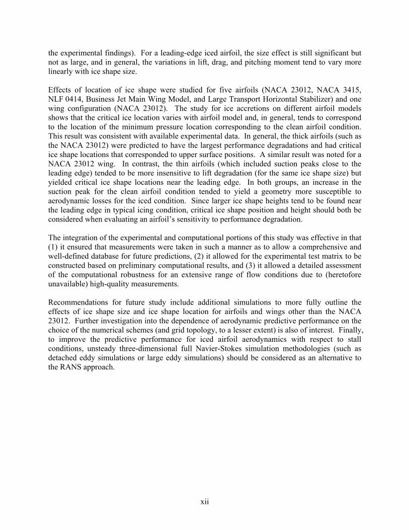
the experimental findings). For a leading-edge iced airfoil, the size effect is still significant but not as large, and in general, the variations in lift, drag, and pitching moment tend to vary more linearly with ice shape size.

Effects of location of ice shape were studied for five airfoils (NACA 23012, NACA 3415, NLF 0414, Business Jet Main Wing Model, and Large Transport Horizontal Stabilizer) and one wing configuration (NACA 23012). The study for ice accretions on different airfoil models shows that the critical ice location varies with airfoil model and, in general, tends to correspond to the location of the minimum pressure location corresponding to the clean airfoil condition. This result was consistent with available experimental data. In general, the thick airfoils (such as the NACA 23012) were predicted to have the largest performance degradations and had critical ice shape locations that corresponded to upper surface positions. A similar result was noted for a NACA 23012 wing. In contrast, the thin airfoils (which included suction peaks close to the leading edge) tended to be more insensitive to lift degradation (for the same ice shape size) but yielded critical ice shape locations near the leading edge. In both groups, an increase in the suction peak for the clean airfoil condition tended to yield a geometry more susceptible to aerodynamic losses for the iced condition. Since larger ice shape heights tend to be found near the leading edge in typical icing condition, critical ice shape position and height should both be considered when evaluating an airfoil‘s sensitivity to performance degradation.

The integration of the experimental and computational portions of this study was effective in that (1) it ensured that measurements were taken in such a manner as to allow a comprehensive and well-defined database for future predictions, (2) it allowed for the experimental test matrix to be constructed based on preliminary computational results, and (3) it allowed a detailed assessment of the computational robustness for an extensive range of flow conditions due to (heretofore unavailable) high-quality measurements.

Recommendations for future study include additional simulations to more fully outline the effects of ice shape size and ice shape location for airfoils and wings other than the NACA 23012. Further investigation into the dependence of aerodynamic predictive performance on the choice of the numerical schemes (and grid topology, to a lesser extent) is also of interest. Finally, to improve the predictive performance for iced airfoil aerodynamics with respect to stall conditions, unsteady three-dimensional full Navier-Stokes simulation methodologies (such as detached eddy simulations or large eddy simulations) should be considered as an alternative to the RANS approach.

xii

1. INTRODUCTION.

Aircraft aerodynamic degradation due to large droplet ice accretion is a severe problem faced by pilots and has caused many accidents. When an aircraft enters a region containing supercooled water droplets, ice accretions of various shapes can form at different locations on its aerodynamic surfaces under different meteorological and flight conditions. The three primary ice shapes encountered are rime ice, glaze ice, and ridge ice (figure 1). Rime ice (with a fairly streamlined round shape shown in figure 1(a)) forms when water droplets freeze on impact and occurs at low liquid water content levels at temperatures well below freezing. Glaze ice (with a more irregular ice shape) forms at temperatures near freezing when some of the water droplets freeze partly on impact and the rest run back. This often results in the development of a horn ice shape, as shown in figure 1(b). Ridge ice can form when the deicing system is activated for the leading edge and large water droplets run back forming ice accretion after the active portion of deicing system on the upper surface (figure 1(c)). This ice shape differs from the other two in that it is an upper surface ice shape, while the others are leading-edge ice shapes. All three ice accretion shapes can cause deterioration in an airfoil‘s aerodynamic performance, especially the glaze and ridge shapes.

(a) Rime Ice Shape (b) Glaze Ice Shape (c) Ridge Ice Shape

FIGURE 1. TYPICAL ICE ACCRETION SHAPES

The ice accretion effect on aerodynamics has been experimentally and numerically studied for many years. The earlier experimental studies on iced airfoils can be traced back to 1940s when several accidents were first diagnosed as being due to aircraft icing [1 and 2]. Experiments have continued leading to a extensive catalog of ice shapes and their effects for a range of conditions. Numerical simulation has become common in the last two decades and is now playing an important role as it is often a less expensive alternate investigation tool. The most popular numerical technique is the Reynolds Averaged Navier-Stokes (RANS) method whereby the viscous turbulent effects are resolved using time-averaged closure models. Previous numerical studies have shown trends similar to those obtained by experiments and as such can give the guidance at other conditions. However, the complex flow fields associated with iced airfoils do not always allow robust predictions with conventional RANS methodologies.

Previous studies have generally focused on rime and glaze ice accretion because they are more common ice shapes. Recently, the ridge ice shapes have been given more consideration because they have been found to yield severe degradation of airfoil performance under certain conditions [3]. In particular, the University of Illinois‘ icing research group has conducted detailed experimental studies on ridge ice accretions using simulated spanwise-step shapes [4-6]. This included an investigation of the effects of the Reynolds number, Mach number, ice shape size, and ice shape location on airfoil aerodynamic performance. These experiments, based on a

1

quarter-round shape on a NACA 23012 airfoil at the NASA Langley Low Turbulence Pressure Tunnel (LTPT), systematically studied Reynolds and Mach numbers effects of airfoils with ice shapes over a significant range of conditions. Additional measurements were obtained in the University of Illinois Urbana, Champaign (UIUC) Low-Speed Wind Tunnel (LSWT) for the NACA 23012 and other airfoils with simulated ridge and leading-edge ice shapes, which further complement the above data set.

Taking advantage of the above unprecedented experimental data set, a parallel numerical investigation on ice shape effect was conducted for various Reynolds and Mach numbers and airfoil and wing geometries. This study had two goals: (1) to provide a systematic view on the ice accretion effects on airfoil and wing aerodynamics and (2) to evaluate the fidelity of conventional RANS using a large range of experimental data and flow conditions.

2. PREVIOUS NUMERICAL STUDIES.

With the dramatic progress of computer technology in recent decades, computational fluid dynamics in the form of steady RANS has made significant improvements in predictive performance. The following discusses some of the two-dimensional (2-D) (airfoil) studies followed by a simple review of a few known three-dimensional (3-D) (wing) studies. A more detailed review of RANS studies of iced airfoils is available in previous publications [7 and 8].

2.1 ICED AIRFOIL RANS SIMULATIONS.

With respect to 2-D RANS simulations for iced airfoils, there have been several investigations. Potapczuk [9] used the ARC2D code on a structured grid to study the aerodynamic effects of leading-edge glaze ice on the NACA 0012 airfoil. Thin layer Navier-Stokes equations were solved with the Baldwin-Lomax algebraic two-layer eddy viscosity model. Predictions for angles of attack between 0 and 10 degrees were presented and compared with experimental data. The lift, drag, and moment results showed good agreement for angles of attack below stall. The pressure distribution was also well simulated, except for the region near the ice shape. For angles of attack above 7 degrees, Potapczuk applied a time-accurate RANS solution to model the unsteady behavior after stall. Averaged pressure values were compared with converged steady-state solution and experiment results. The predictions were improved but there were still significant deviations from the experiment.

Caruso, et al. [10 and 11] applied RANS with unstructured grids along the leading-edge ice shape with high resolution using a hole-remeshing approach with Navier-Stokes equations. The predicted flow field of the unstructured grid solutions compared well with predictions obtained on structured grid though no comparison with experiment was available. With the adaptability of unstructured grids, this method demonstrated that ice growth could be calculated as a function of time while simultaneously solving for the flow field.

Dompierre, et al. [12] reported results of computations about iced airfoil using adaptive meshing techniques. An efficient remeshing technology was employed so that the Navier-Stokes equations could be solved on a grid with a uniform distribution error. The Finite Volume Galerkin method was applied for iced airfoils using the k- ε turbulence model with wall functions. A number of ice shapes were considered for the NACA 0012 airfoil, including

2

leading-edge ice horns, an upper surface quarter-round ridge, and small-scale roughness. The computations were performed at Re = 3.1x106 and M = 0.15. The mesh was shown to appropriately adapt to the predicted viscous regions. Although flow field descriptions and a lift curve were obtained, no experimental data was available for comparison. The computations revealed a very large loss of lift due to ridge ice shape, much greater than that due to leading-edge ice accretion.

In 1999, extensive experimental data (lift, drag, aerodynamic moment, hinge moment, and pressure distribution) for upper surface spanwise-step ice shapes and leading-edge horn ice shapes became available through the work of Bragg, Lee, and Kim, et al. [4-6], which made possible a detailed comparison of the aerodynamic aspects mentioned above. Dunn and Loth [13] presented the first detailed comparison of these data with computational predictions based on a 2-D unstructured full Navier-Stokes solver, NSU2D. Simulations were concentrated on an upper surface spanwise-step ice accretion represented by a quarter-round shape on a modified NACA 23012 airfoil. Numerical results yielded good agreement with experimental data up to the stall conditions, and the ice shape size and location effects were reasonably predicted with respect to the force, pitching moment, and hinge moment data. Figures 2 and 3 show a sample NSU2D lift and drag prediction for a modified NACA 23012 airfoil with an upper surface ice shape. Later, Kumar and Loth [14] extended this study to several other airfoil geometries from the NASA Glenn Research center Modern Airfoil Program. In particular, the NACA 23012, NLF 0414, the Business Jet Main Wing Model (BJMW), and the Commercial Transport Horizontal Tailplane Model were studied, and it was found that the critical ice location was sensitive to the airfoils‘ clean aerodynamic load distribution.

Cl

α(deg)

FIGURE 2. LIFT COEFFICIENT FOR A NACA 23012M AIRFOIL WITH k/c = 0.0083 QUARTER-ROUND ICE SHAPE LOCATED AT x/c = 0.1

3

Cl

Cd

FIGURE 3. DRAG COEFFICIENT FOR A NACA 23012M AIRFOIL WITH k/c = 0.0083 QUARTER-ROUND ICE SHAPE LOCATED AT x/c = 0.1

None of the previous 2-D RANS simulations on iced airfoils included detailed investigation with respect to the effects of Reynolds and Mach numbers. This is probably due to the fact that very limited experimental data studying these effects were previously available. However, the present UIUC experiments have now systematically investigated the airfoils‘ aerodynamic degradation for a large variety of Reynolds and Mach numbers, airfoil models, ice shape sizes, ice shape locations, and ice shapes geometries. As such, it is important and now possible to assess the computational fidelity of RANS to predict the aerodynamics for a wide range of flow and geometrical conditions.

2.2 ICED WING RANS SIMULATIONS.

With respect to 3-D RANS efforts, a simulation of a finite wing with leading-edge ice shape was conducted by Kwon, et al. [15 and 16]. Flow fields of the wings with a NACA 0012 airfoil section in both rectangular and swept wing configurations were simulated by solving full 3-D Navier-Stokes equations on a structured C-type grid. The results showed the chordwise pressure predictions are quite good at α = 4° and α = 8° at several spanwise locations compared to the experimental results [17], but it was also found that the boundary condition of a computational sidewall played an important role in the prediction accuracy.

Chung, et al. [18] performed a 3-D Navier-Stokes computation on a NACA 23012 wing section with upper surface ice accretion. An ice shape with a height to chord ratio (k/c) of 0.0074 was selected based on the smoothed Icing Research Tunnel measured shapes for this wing. A full Navier-Stokes solver, NPARC, was used for the simulation with a two-block C-type grid generated by commercial grid generation software Gridgen. Both the Baldwin-Barth and the Spalart-Allmaras turbulence models were used, but no experimental data was available for comparison. While a leading-edge stall at an angle of attack of 9 degrees was predicted in the

4

2-D computation, a 13 degree stall angle with a trailing-edge stall was found for the 3-D simulation. This indicated significant modification of the stall behavior between iced airfoils and iced wings, at least for upper surface ridge ice shapes. It was also concluded by the authors that more work is needed in 3-D ice shape modeling and in grid refinement to understand the difference between 2-D and 3-D results.

While such studies have showed that there can be a significant difference between airfoil and wing geometries, there have been no iced wing studies that have examined the sensitivity to ice shape location. This is of significant interest since it is not known if 3-D effects will modify the critical ice shape location as predicted for the airfoil case.

3. COMPUTATIONAL METHODOLOGY.

The accuracy and reliability of simulations is dependent on the numerical aspects employed. The selection of the appropriate spatial and temporal discretization scheme, turbulence model, and computational grid topology can have a significant influence on the final simulation results. Each choice of a methodology aspect can have benefits and disadvantages. For example, a high-order scheme is thought to provide more accurate predictions, however, it may be more unstable compared to a low-order scheme. Also, one- and two-equation turbulence models are preferred over algebraic models in terms of accuracy but come at a price of more computing time.

With respect to grid topology, structured grids are more efficient and preferred in the boundary layer region along the airfoil surface, but unstructured grids require fewer grid points outside the boundary layer region. Considering an irregular-iced airfoil geometry, unstructured grids are easier to generate and also are more easily adapted to flow gradients. But structured grids allow efficient computation and parallelization. In addition, the structured grid approach is more typically used in industry. As such, a structured Navier-Stokes equation solver WIND [19] was primarily applied in this study. The WIND code is also chosen because it is has become the core methodology of the NASA Glenn Research Center. However, a commercial software package, FLUENT [20], which works on both structured and unstructured grids, is applied herein for a few cases to examine variations in simulation results between different grid topologies and different computational fluid dynamics code packages.

Notably, both WIND and FLUENT are finite-volume methods based on full Navier-Stokes equations with a Boussinesq assumption for turbulence. WIND uses a mapped computation grid for establishing transformed coordinate directions and the integral form of flow and is similar to a finite difference method as it is structured grid-based. However, FLUENT uses cell faces for integration since it must handle structured grids as well as hybrid meshes containing quadrilateral and triangular cells. Since FLUENT supports multielement unstructured grid types, its discretization of the RANS equations is also processed differently with WIND.

3.1 NAVIER-STOKES EQUATIONS.

For both WIND and FLUENT, the unsteady governing equations of compressible viscous flow in three dimensions in Cartesian coordinates can be represented as follows, using tensor notation

5

∂q +∂f i ∂ri (1)=

∂t ∂xi ∂xi

where

qi = (ρ, ρui , E )T

f i = (ρui , ρuiu j + pδij ,(E + p)ui )T (2)

ri = (0,τ ij ,u jτ ij − Qi ) T

Using Stokes‘ hypothesis and modeling the Reynolds stress and heat flux terms with the Boussinesq assumption, the viscous stress tensors and heat flux vectors have the form of

τ ij = (µ + µ t )[( ∂ui +

∂u j ) − 2 ∂uk

∂x j ∂xi 3 ∂xk

δ ij ] (3)

and

∂ p γ ( µ + µt ) ρ (4)Qi = −

γ −1 Pr Prt ∂xi

3.2 SIMULATION PROGRAMS.

3.2.1 Overview of WIND.

WIND is a structured Navier-Stokes equation solver using a node-centered finite-volume approach. The Navier-Stokes equations were first transformed from physical Cartesian coordinate system (x,y,z) to a computational generalized coordinate system (ξ, η, ζ) in which grid spacing is normalized. The governing equations in the new coordinate system are represented as

∂Q ∂F ∂G ∂H ∂R ∂S ∂T+ + + = + +∂t ∂ξ ∂η ∂ζ ∂ξ ∂η ∂ζ

(5)

In WIND, the transformed Navier-Stokes equations are written in conservative delta law form as follows:

[I + ∆tδξ A − ∆tδξ M ][I + ∆tδη B − ∆tδη N ][I + ∆tδζ C − ∆tδζ O] ⋅ ∆Q =

− ∆t[δξ E +δη F +δζ G −δξ R −δη S −δζ T ] (6)

where

∂E ∂F ∂G ∂R ∂S ∂TA =∂Q

B =∂Q

, C =∂Q

and M =∂Q

N =∂Q

, O =∂Q

(7)

6

For the simulations included herein, a Roe second-order upwind scheme (specialized for stretched grids) is selected to discretize the convection terms on the right-hand side of the equations. This scheme was chosen because it was considered the most robust scheme with favorable accuracy available in WIND. The steady-state solution was generally obtained with a local Courant-Fredrichs-Levy number of 1.3 to insure the numerical stability as well as to accelerate the convergence. Only fully converged RANS results are presented, where convergence was recorded when the norm residue reaches a level 10-6 or lower.

3.2.2 Overview of FLUENT.

FLUENT uses a control volume-based technique to convert the governing equations to algebraic equations that can be solved numerically. This control volume technique consists of integrating the governing equations about each control volume, yielding discrete equations that conserve each quantity. The discretization of the governing equations is similar to that of NSU2D [8 and 21], except that elements with more sides are considered and the integrations are taken along all the side faces. The flow property values are stored at the cell center. The face value, which is needed for the element flux integration, is derived from the cell center value. In this study, a second-order upwind scheme was applied in the computation for clean airfoil flows, while both first-order and second-order solvers were used for the iced airfoil cases.

When the first-order upwind scheme is employed, this value is simply taken from its upwind cell. And for the second-order upwind scheme, the value was obtained as

φf =φ + ∇ φ• ∆s (8)

Here ∆s is the distance from the cell center to face center and the gradient is calculated using the divergence theorem, which in discrete form is written as

→

∑ φf L (9)∇ φ = 1 ∫∫ ∇ φ • dS = 1

∫φ • d L = 1 N faces ~ r A A A f

~ Where φf is computed by averaging φ from the two cells adjacent to the face. Similar to NSU2D, the diffusion terms are central-differenced and are always second-order accurate.

3.3 TURBULENCE MODELS AND TRANSITION.

The quality of the turbulence model is important to the RANS flow predictions, especially for high Reynolds number flow problems. For the complex turbulent flow around iced airfoils, simple algebraic turbulence models generally are not thought to be accurate enough to describe all the turbulent flow phenomena including transport properties, boundary layer profiles, etc. Thus, most recent work has focused on one-equation and two-equation models. To compare the quality of these models, selected cases were simulated with different turbulence models, including the Spalart-Allmaras one-equation model, the Baldwin-Barth one-equation model, the Mentor Shear Stress Transport (SST) two-equation model, and the k-ε two-equation model, etc.

7

The Spalart-Allmaras model was chosen as the baseline turbulence model because of its good performance in the comparisons and previous studies [13 and 14].

3.3.1 Spalart-Allmaras Turbulence Model.

The Spalart-Allmaras model was developed in 1992 with the aim of high Reynolds number aerodynamics flow simulations [22]. The one-equation Spalart-Allmaras model was designed for aerodynamic flows and was calibrated on mixing layers, wakes, and boundary layers. It was first applied in airfoil computations and gave good results. Later it was adopted in many other flow problems such as tunnel flow, cylinder flow, and iced airfoil flow simulations. Due to its performance under different flow conditions (some are especially complex), the Spalart-Allmaras model is thought to be one of the most successful turbulence models among the available one- and two-equation RANS models [23], and it appears well suited for iced airfoil flows. The model employs a partial difference equation for the modified eddy viscosity ῦ as

~ ~ ~ ~ 1 ~ ~ ~Dν = Cb1 [1− f t 2 ] Sν +

σ[ ∇ ((ν +ν )∇ ν + Cb 2 ( ∇ ν )2 ] − [Cw1 f w −

Cb1 f t 2 ][ ν ] 2 + f t1∆U (10)Dt k 2 d

where the relation between this working variable and the turbulent kinematic eddy viscosity is ~ν t =ν fν 1 , and where the wall function is defined as

χ 3

fν 1 = χ 3 + cv13

and

~ χ = ν

ν

is the ratio of modified eddy viscosity to kinematic viscosity.

The Spalart-Allmaras model considers the influence of turbulence production, transportation, wall destruction, diffusion and trip location, and models each of these phenomena based on

~ empirical relationships. The D denotes the substantial derivative. The quality S in the

Dt production term is given by

~ ~ νS = S +κ 2d 2 fν 2

(11)

where the source term, S, is modeled with the magnitude of the vorticity

S = ω = ∂v − ∂u (12)∂x ∂y

and d in the wall destruction term is the distance to the closest wall.

8

The auxiliary equations appearing in the above equation are

χ 6 ~νfν 2 = 1 − 1 + χfν 1

; f w = g

16

+ cw 63 ; g = r + cw2 (r 6 − r); r =

S ~ k 2 d 2 (13)

g + cw3

and the constants as specified in reference 22 are

Cb1 = 0.1355, Cb2 = 0.622, Cv1 = 7.1, σ = 2/ 3, Cw2 = 0.3, Cw3 = 2.0, κ = 0.41 (14)

3.3.2 Other Turbulence Models.

The Baldwin-Barth one-equation model and the Mentor SST model were also applied in selected simulations to compare the performance with the Spalart-Allmaras turbulence model. While other turbulence models, such as the Thomas algebraic shear layer model and the Chien k-ε two-equation model, were also tried, they did not consistently provide converged results and, thus, are not discussed here.

The Baldwin-Barth model is a popular one-equation turbulence model developed earlier than the Spalart-Allmaras model and has been applied for many turbulent flow predictions. In this model, the eddy viscosityν t is express as

ν t = C µνR T D 1 D 2 (15)

where the turbulent Reynolds number is given as

k 2

RT = νε

(16)

The Baldwin-Barth model applies an eddy viscosity partial difference equation similar to the Spalart-Allmaras model.

D(νRT ) = [Cε 2 f 2 − Cε 2 ](νRT P)1/ 2 + (ν + ν t )∇ 2 (νRT ) − 1 ∇ ν t ∇ (νRT ) (17)

Dt σ ε σ ε

where

Cε1 = 1.2, Cε 2 = 2.0, C = 0.09, A0 + = 26, A2 + = 10, 1 = [Cε1 − Cε 2 ]Cµ

1 / 2 / k 2 , κ = 0.41 (18)σε

9

and

P =ν t [( ∂Ui +

∂U j ) ∂Ui − 2 ∂U k ∂U k ],

∂x j ∂xi ∂x j 3 ∂xk ∂xk

D1 = 1 − exp(− y + / A0 + ) and D2 = 1 − exp(− y + / A2

+ ), (19) +yf 2 =

Cε1 + [1 − Cε1 ][ 1

+ + D1 D2 ][(D1 D2 )1/ 2 + (D1 D2 )1/ 2 ][

D + 2 exp(− y + / A0

+ ) + D

+ 1 exp(− y + / A2

+ )Cε 2 Cε 2 κy A0 A2

The Mentor SST two-equation model was developed to combine the advantages of the k-ω model in the near wall region and k-ε model in the free-shear and outer flow regions. In this model, the eddy viscosity is defined as the function of kinetic energy, k, and specific dissipation rate of turbulent frequency, ω, as

µ t = max [ 1;

ρΩ kF/

2

ω /( a1ω )]

with a1 = 0 .31 (20)

where Ω is the absolute value of vorticity and F2 is an auxiliary function to limit the maximum value of the eddy viscosity in the turbulent boundary layer as

500 ; µ k 2

(21)F2 = tanh

max 2

0.09ωy ρy 2ω

The two transport equations of the model are defined below with a blending function F1 for the model coefficients of the original ω and ε model equations. The transport equation for kinetic energy is

∂( ρk ) + ∂∂ x j ρu j k − (µ + σ k µ t ) ∂

∂ xk

j

= [2µ t (Sij − Skkδ ij / 3)− 2ρkδ ij / 3]Sij − β * ρϖk (22)∂t

and the transport equation for the specific dissipation of turbulence is

∂( ρϖ ) + ∂∂ x j ρu jω − (µ +σ ω µ t )

∂ω = Pω − βρω2 + 2(1 − F1 )

ρσω2 ∂k ∂ω (23)∂t ∂x j ω ∂x j ∂x j

where the last term represents the cross-diffusion term that transformed from original ε equations, and the production term of ω can be approximated as proportional to the absolute value of vorticity as

Pω = 2γρ( Sij −ωSkkδ ij / 3 )Sij ≈ γρΩ 2 (24)

10

The auxiliary function F1 is defined as

2 4500 k

;; k ωρσµ 4 F1 = tanh min

max

2

0 .09ωy ρy 2ω CD kω y 2 (25)

where

CD kω = max 2 ρσ ω 2 ∂k ∂ω ; 10 − 20

(26)

ω ∂x j ∂x j

The constants of the Mentor SST model are a1 = 0.31, β = 0.09, κ = 0.41, and the model coefficients β, γ, σk, σω, denoted with Φ, are defined by blending the coefficients of the original k-ω model, denoted as Φ1, with those of the transformed k-ε model, denoted as Φ2: Φ = F1Φ1 + (1- F1)Φ2, where Φ = β, γ, σk, σω with the coefficients of the original k-ω and k-ε models defined as

*σ k1 = 0.85,σω1 = 0.85, β1 = 0.075,γ1 = β1 / β −σω1k 2 / *β = 0.553 (27)

*σ k 2 = 1.0,σω2 = 0.856, β2 = 0.0828,γ1 = β1 / β −σω1k 2 / *β = 0.440 (28)

3.3.3 Transition Point Specification.

In this study, transition points for the clean airfoil cases were based on the most upstream position of two locations: (1) the location of a trip strip (generally placed at 5% on lower surface and 2% on upper surface in experiments) and (2) the transition point location given by the integral boundary layer program of XFOIL (which incorporates an en-type amplification formulation) [24-26]. For the iced airfoils, the transition points were specified based on the most upstream position of three locations: (1) the location of a trip strip, (2) the transition point predicted for the counterpart clean airfoil at an equivalent lift, and (3) the ice shape location.

3.4 GRID GENERATION AND BOUNDARY CONDITIONS.

A single-block O-type grid is generated from the airfoil surface to 20 chords length away in all directions by using the grid generator software, Gridgen. In this software, an elliptical is solved using a Successive Over Relaxation numerical scheme to improve the grid distribution quality. The nondimensional first grid spacing in the normal direction is set as 2*10-6, consistent with a y+ of about 1 for all flow conditions. In general, 400 points are distributed along the airfoil surface (with about 100 points along the ice shape), and 100 points are assigned in the normal direction. The grid distribution is clustered on the region where high flow-field gradients are expected, such as the leading edge, trailing edge, and ice shape locations. A typical computational grid for an iced airfoil is shown in figure 4.

11

The boundary conditions are specified through Grid MANagement for WIND and GAMBIT for FLUENT. All cases include a viscous wall boundary condition on the airfoil (or wing) surface and free-stream boundary condition on the far-field boundary.

(a) Far-Field View

(b) Close-Up View

FIGURE 4. TYPICAL GRID FOR AN ICED NACA 23012 AIRFOIL

12

4. RESULTS AND DISCUSSION.

4.1 ASSESMENT OF NUMERICAL PARAMETERS.

In order to access the properties of the WIND code, such as the grid sensitivity, the turbulence model, effect, and 3-D capability, simulations were first completed with selected clean and iced airfoil and wing cases for various grid resolutions, numerical schemes, and turbulence models. Results were compared with LTPT experimental data or previous reported simulation and experimental results.

4.1.1 Grid Dependence Sensitivity for Clean NACA 23012 Airfoil.

To evaluate the grid sensitivity and optimization, WIND was validated for a clean NACA 23012 airfoil at baseline LTPT experimental condition of M = 0.12 and Re = 10.5x106. The grid dependence study was performed in both parallel and normal directions to the airfoil surface.

In total, four grids (300 x 100, 400 x 100, 400 x 50, and 400 x 200) were tested for this validation purpose. In all cases, the first grid point normal to the surface was at a distance of 2x10-6 chord length, which corresponds to a y+ of about 1 near mid-chord. Figures 5-7 show the lift curve, drag, and moment coefficient distributions for the clean NACA 23012 airfoil with different grid resolutions, as well as the experimental LTPT results of Broeren [27].

In general, the aerodynamic coefficients are well predicted for all the grids, except for the 400 x 50 grid. Increasing the grid points along the streamwise direction from 300 to 400 yields no notable difference for the predicted lift, moment, and drag curves. As for normal direction sensitivity, there are no significant differences between the predictions with 100 and 200 points. However, 50 grid points was found to be too coarse to describe the flow gradients and boundary layer properties, especially at higher angles of attack.

Figure 8 shows the pressure distribution at α = 15° for grids with different resolutions. While the suction pressure prediction based on the coarsest 400 x 50 grid is somewhat low on the upper surface, there is no obvious difference among the results for the three finer grid resolutions. The slightly underpredicted pressure distribution with the 400 x 50 grid leads to the significantly lower Cl prediction.

Although a 300 x 100 grid was found sufficient for all the aerodynamic predictions (force coefficients and pressure distributions), a 400 x 100 grid was chosen as the baseline grid with the consideration that the complex flow field around airfoil will require more grid resolution around ice shapes.

13

2

1.5

1

0.5

0

-0.5

-1-10 -5 0 5 10 15 20

LTPT Data WIND-RANS-300x100 WIND-RANS-400x100

α (deg)

(a) With Variation in Streamwise Direction

2

1.5

1

0.5

0

-0.5

-1-10 -5 0 5 10 15 20

LTPT Data WIND-RANS-400x50 WIND-RANS-400x100 WIND-RANS-400x200

α (deg)

(b) With Variation in Normalwise Direction

FIGURE 5. LIFT COEFFICIENT FOR A CLEAN NACA 23012 AIRFOIL AT Re = 10.5X106, M = 0.12

lC

l C

14

0.2

0.18

0.16

0.14

0.12

0.1

0.08

0.06

0.04

0.02

0-10 -5 0 5 10 15 20

LTPT Data WIND-RANS-300x100 WIND-RANS-400x100

α (deg)

(a) With Variation in Streamwise Direction

0.2

0.18

0.16

0.14

0.12

0.1

0.08

0.06

0.04

0.02

0-10 -5 0 5 10 15 20

LTPT Data WIND-RANS-400x50 WIND-RANS-400x100 WIND-RANS-400x200

α (deg)

(b) With Variation in Normalwise Direction

FIGURE 6. DRAG COEFFICIENT FOR A CLEAN NACA 23012 AIRFOIL AT Re = 10.5x106, M = 0.12

dC

d C

15

0.1

0.08

0.06

0.04

0.02

0

-0.02

-0.04

-0.06

-0.08

-0.1-10 -5 0 5 10 15 20

LTPT Data WIND-RANS-300x100 WIND-RANS-400x100

α (deg)

(a) With Variation in Streamwise Direction

0.1

0.08

0.06

0.04

0.02

0

-0.02

-0.04

-0.06

-0.08

-0.1-10 -5 0 5 10 15 20

LTPT Data WIND-RANS-400x50 WIND-RANS-400x100 WIND-RANS-400x200

α (deg)

(b) With Variation in Normalwise Direction

FIGURE 7. PITCHING-MOMENT COEFFICIENT FOR A CLEAN NACA 23012 AIRFOIL AT Re = 10.5x106, M = 0.12

m

C

C

m

16

-10

-8

-6

-4

-2

0

2 -0.2 0 0.2 0.4 0.6 0.8 1 1.2

LTPT Data WIND-RANS:300x100 WIND-RANS:400x100 WIND-RANS:400x50 WIND-RANS:400x200

x/c

FIGURE 8. PRESSURE DISTRIBUTION FOR A CLEAN NACA 23012 AIRFOIL AT Re = 10.5x106, M = 0.12, α = 15°

4.1.2 Turbulence Model Sensitivity and Selection.

The RANS prediction quality can be sensitive to the choice of the turbulence model. In WIND, there are many options for the turbulence model selection, including algebraic, one-equation, and two-equation models. Three representative and commonly used models, the Baldwin-Barth one-equation turbulence model, the Spalart-Allmaras one-equation turbulence model, and the Mentor SST two-equation turbulence model, were selected to evaluate their capability with the iced airfoil flows. Predictions for lift, drag, and pitching-moment coefficients based on those models are shown in figures 9-11.

C p

17

1

0.8

0.6

0.4

0.2

0

-0.2

-0.4

-0.6-10 -5 0 5 10 15 20

LTPT Data WIND-RANS-S-A WIND-RANS-B-B WIND-RANS-SST

α (deg)

FIGURE 9. LIFT COEFFICIENT FOR AN ICED NACA 23012 AIRFOIL AT Re = 10.5x106, M = 0.12

0.35

0.3

0.25

0.2

0.15

0.1

0.05

0 -10 -5 0 5 10 15 20

α (deg)

LTPT Data WIND-RANS-S-A WIND-RANS-B-B WIND-RANS-SST

C d

Cl

FIGURE 10. DRAG COEFFICIENT FOR AN ICED NACA 23012 AIRFOIL AT Re = 10.5x106, M = 0.12

18

0.02

0

-0.02

-0.04

-0.06

-0.08

-0.1-10 -5 0 5 10 15 20

LTPT Data WIND-RANS-S-A WIND-RANS-B-B WIND-RANS-SST

α (deg)

FIGURE 11. PITCHING-MOMENT COEFFICIENT FOR AN ICED NACA 23012 AIRFOIL AT Re = 10.5x106, M = 0.12

As seen in the figures, the Baldwin-Barth turbulence model generally does not provide as good results as the other two models. Results based on the Spalart-Allmaras and Mentor SST models are close to each other for the drag and moment predictions. However, the lift predicted with the Spalart-Allmaras model is more representative of the experimental data up to the experimental stall angle. At negative angles of attack, the Spalart-Allmaras model is also quite reasonable for the pitching moment predictions. In addition, as a one-equation model, Spalart-Allmaras model takes less time for computation than two-equation Mentor SST model. Due to its reasonable performance for iced airfoil flows and affordable cost, the Spalart-Allmaras model was selected as the baseline turbulence model in this study. However, it should be noted that the choice of the turbulence model yielded large variations in the results and that no single model was entirely robust.

4.1.3 Assessment for Clean and Iced Wings.

The 3-D validation for the WIND code is conducted for a rectangular NACA 0012 wing at M = 0.12 and Re = 1.5x106, and both clean and leading-edge iced shape conditions were considered. The results are compared to Khodadoust and Bragg‘s experimental data [17] and Kwon and Sankar‘s simulation results [16]. The three-zone grid has a resolution comparable with that of Kwon and Sankar, although a finer spanwise resolution was included herein. The grid configuration for clean NACA 0012 wing is shown in figure 12 with a resolution of 208*61*26 in the main wing zone (covering the wing surface), 58*48*11 in the second zone (inner zone for region extended from tip), and of 208*61*11 in the third zone (outer zone for region extended from tip). For iced NACA 0012 wing, while the same number of grid points were used in the normal and spanwise direction, ten more points were added along the chordwise direction to keep a similar grid distribution as in the clean case. The WIND code was run in parallel on the UIUC 208 dual-processor machine clusters for all the 3-D computations.

Cm

19

Zone 1

Zone 3

Zone 2

FIGURE 12. THREE-DIMENSIONAL GRID FOR A RECTANGULAR CLEAN NACA 0012 WING

The validation cases were calculated at an angle of attack of 8 degrees for the clean wing and at 4 and 8 degrees for iced wing. Figure 13 shows the sectional Cl prediction at different spanwise locations for the clean wing. Despite the slight overprediction near the tip, the performance of the present simulation is reasonable and comparable to that of Kwon and Sankar‘s predictions.

0.8

0.7

0.6

0.5

0.4

0.3

0.2 0 0.2 0.4 0.6 0.8 1

LSWT-Data WIND-3D KWON & Sankar

Spanwise location (2y/b)

FIGURE 13. SECTIONAL LIFT ALONG THE SPAN FOR A CLEAN NACA 0012 WING AT Re = 10.5x106, M = 0.15, α = 8°

The pressure coefficients at the midspan are compared in figure 14. The agreement between WIND prediction and experimental data is quite good, except for a slight underprediction of the suction peak, which was also noted in Kwon‘s simulations.

Cl

20

-3

-2.5

-2

-1.5

-1

-0.5

0

0.5

1

1.5

LSWT-Data WIND-3D Kwon & Sankar

-0.2 0 0.2 0.4 0.6 0.8 1 1.2

x/c

FIGURE 14. PRESSURE DISTRIBUTION FOR THE MIDSPAN OF A CLEAN NACA 0012 WING AT Re = 10.5x106, M = 0.15, α = 8°

For the iced NACA 23012 wing, figure 15 shows the sectional lift coefficient at different spanwise locations for the two angles of attack. At the lower angle of attack of 4 degrees, the predicted lift value fits the experimental data quite well. However, there is somewhat of an overprediction for the angle of attack of 8 degrees (presumably since it is close to the stall angle of attack). Compared with Kwon and Sankar‘s simulation, the present predictions tend to have a better performance, especially for the section lift near the root plane at 8 degrees. This may be attributed to the finer grid resolution in the spanwise direction applied in this study for which 26 points were distributed (compared to Kwon and Sankar‘s 14 points). Also, there may be differences in the numerical schemes within the applied Navier-Stokes equation solvers.

1

0.9

0.8

0.7

0.6

0.5

0.4

0.3

0.2

0.1

0 0 0.2 0.4 0.6 0.8 1

LSWT-Data WIND-3D KWON & Sankar

α = 4o

α = 8o

Spanwise location (2y/b)

C l

Cp

FIGURE 15. SECTIONAL LIFT ALONG THE SPAN FOR AN ICED NACA 0012 WING AT Re = 10.5x106, M = 0.15, α = 4° (8°)

21

Figures 16 and 17 show the pressure distributions at the midspan section. While the upper surface suction peak and reattachment are well predicted for 4 degrees, they are overpredicted for 8 degrees, indicating an inability to accurately predict the large separation region aft of the ice shape that is associated with stall.

In the 3-D validation cases, the WIND code reasonably predicted the section lift and pressure distribution for both clean and iced NACA 0012 wing configurations. Compared with a previous numerical study by Kwon and Sankar, the present WIND results tend to show a similar, but somewhat better, performance.

-3.5

-3

-2.5

-2

-1.5

-1

-0.5

0

0.5

1

1.5

LSWT-Data WIND-3D Kwon & Sankar

-0.2 0 0.2 0.4 0.6 0.8 1 1.2 x/c

FIGURE 16. PRESSURE DISTRIBUTION FOR THE MIDSPAN OF AN ICED NACA 0012 WING AT Re = 10.5x106, M = 0.15, α = 4°

-3

-2.5

-2

-1.5

-1

-0.5

0

0.5

1-0.2 0 0.2 0.4 0.6 0.8 1 1.2

LSWT-Data WIND-3D Kwon & Sankar

x/c

FIGURE 17. PRESSURE DISTRIBUTION FOR THE MIDSPAN OF AN ICED NACA 0012 WING AT Re = 10.5x106, M = 0.15, α = 8°

22

C p

C

p

4.1.4 Assessment of WIND vs FLUENT.

The characteristics of the WIND code were compared to a different Navier-Stokes equation solver for a few clean and iced NACA 23012 airfoil cases. In particular, numerical simulations were performed with FLUENT at the baseline LTPT experimental conditions, i.e., M = 0.12 and Re = 10.5x106. Since it can employ both structured grids and unstructured grids, FLUENT was used with both grid types to examine the possible grid topology effect on simulation results. The structured grid used with FLUENT is exactly the same one used in the WIND simulations, while the unstructured grid was developed from the structured grid by keeping the boundary layer grids fixed and regenerating the outer region with the triangle grids.

For the clean NACA 23012 cases, FLUENT was run with a second-order space discretion scheme, and for the iced NACA 23012 simulations, FLUENT was run with both first- and second-order schemes (since the second-order scheme was not easy to converge due to the complex flow condition around the ice shape). These FLUENT simulation results were compared with WIND predictions and the LTPT experimental data.

Figures 18 and 19 show the pressure distributions for the clean NACA 23012 airfoil at 0 and 10 degrees angles of attack. Pressure distribution predicted by FLUENT with the same structured grid applied shows no difference compared with WIND (structured grid) result at both angles of attack. There also is no discernable difference for the FLUENT results between structured and unstructured grids, indicating the grid topology effect is negligible for the clean airfoil case.

-1.5

-1

-0.5

0

0.5

1

1.5 -0.2 0 0.2 0.4 0.6 0.8 1 1.2

LTPT-Data WIND-Structured FLUENT-Structured

x/c

Cp

FIGURE 18. PRESSURE DISTRIBUTION FOR A CLEAN NACA 23012 AIRFOIL AT Re = 10.5x106, M = 0.12, α = 0° WITH SECOND-ORDER SCHEMES

23

-5

-4

-3

-2

LTPT-Data WIND-Structured FLUENT-Structured FLUENT-Unstructured

C p

-1

0

1

2-0.2 0 0.2 0.4 0.6 0.8 1 1.2

x/c

FIGURE 19. PRESSURE DISTRIBUTION FOR A CLEAN NACA 23012 AIRFOIL AT Re = 10.5x106, M = 0.12, α = 10° WITH SECOND-ORDER SCHEMES

Figures 20 and 21 show the pressure distribution comparisons for the iced NACA 23012 airfoil with k/c = 1.39% ice shape at x/c = 0.10 at an angle of attack of 0 degrees. Both first- and second-order spatial discretization schemes were considered in these simulations. With a first-order scheme applied, both WIND and FLUENT give poor predictions compared to the experimental values, although FLUENT shows a better prediction before the ice shape. Notably, there is no significant difference between the predictions based on the FLUENT structured versus unstructured grids in either figure. This again indicates that grid topology is not critical as long as high spatial resolution is maintained.

With the second-order scheme applied (figure 21), significant pressure distribution improvements were noted for both the WIND and FLUENT predictions, especially before the ice shape. However, after the ice shape, the pressure is somewhat underpredicted in FLUENT (as in previous NSU2D predictions) and somewhat overpredicted in WIND. It should also be noted that the second-order FLUENT scheme is segregated. Although FLUENT (and NSU2D) provides a better pressure distribution, WIND provides a better lift prediction since the overpredicted pressure after the ice shape is somewhat balanced out by the underpredicted pressure further downstream in the reattaching process.

In summary, the WIND second-order scheme reasonably predicted the flow aerodynamic force coefficients compared to FLUENT. The FLUENT predictions show that the grid topology effect is not very significant if the same discretion and interpolation method is applied. With structured grids applied, the WIND second-order upwind scheme was chosen as the baseline scheme for the present iced airfoil and wing flow studies.

24

-4

-3

-2

-1

0

1

2-0.2 0 0.2 0.4 0.6 0.8 1 1.2

LTPT Data WIND-Structured FLUENT-Structured FLUENT-Unstructured

x/c

FIGURE 20. PRESSURE DISTRIBUTION FOR AN ICED NACA 23012 AIRFOIL (k/c = 1.39%, x/c = 0.10) AT Re = 10.5x106, M = 0.12, α = 0° FOR

FIRST-ORDER SCHEMES

-3

-2.5

-2

-1.5

-1

-0.5

0

0.5

1

1.5 -0.2 0 0.2 0.4 0.6 0.8 1 1.2

LTPT Data WIND-Structured FLUENT-structured FLUENT-Unstructured

x/c

FIGURE 21. PRESSURE DISTRIBUTION FOR AN ICED NACA 23012 AIRFOIL (k/c = 1.39%, x/c = 0.10) AT Re = 10.5x106, M = 0.12, α = 0° WITH

SECOND-ORDER SCHEMES

Cp

Cp

25

4.2 EFFECT OF REYNOLDS NUMBER FOR NACA 23012 AIRFOIL.

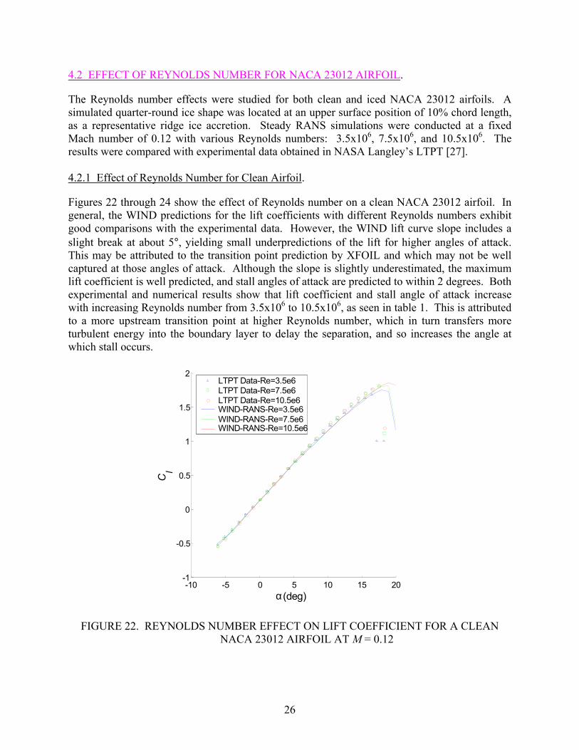
The Reynolds number effects were studied for both clean and iced NACA 23012 airfoils. A simulated quarter-round ice shape was located at an upper surface position of 10% chord length, as a representative ridge ice accretion. Steady RANS simulations were conducted at a fixed Mach number of 0.12 with various Reynolds numbers: 3.5x106, 7.5x106, and 10.5x106. The results were compared with experimental data obtained in NASA Langley‘s LTPT [27].

4.2.1 Effect of Reynolds Number for Clean Airfoil.

Figures 22 through 24 show the effect of Reynolds number on a clean NACA 23012 airfoil. In general, the WIND predictions for the lift coefficients with different Reynolds numbers exhibit good comparisons with the experimental data. However, the WIND lift curve slope includes a slight break at about 5°, yielding small underpredictions of the lift for higher angles of attack. This may be attributed to the transition point prediction by XFOIL and which may not be well captured at those angles of attack. Although the slope is slightly underestimated, the maximum lift coefficient is well predicted, and stall angles of attack are predicted to within 2 degrees. Both experimental and numerical results show that lift coefficient and stall angle of attack increase with increasing Reynolds number from 3.5x106 to 10.5x106, as seen in table 1. This is attributed to a more upstream transition point at higher Reynolds number, which in turn transfers more turbulent energy into the boundary layer to delay the separation, and so increases the angle at which stall occurs.

2

1.5

1

0.5

0

-0.5

-1 -10 -5 0 5 10 15 20

α (deg)

LTPT Data-Re=3.5e6 LTPT Data-Re=7.5e6 LTPT Data-Re=10.5e6 WIND-RANS-Re=3.5e6 WIND-RANS-Re=7.5e6 WIND-RANS-Re=10.5e6

FIGURE 22. REYNOLDS NUMBER EFFECT ON LIFT COEFFICIENT FOR A CLEAN NACA 23012 AIRFOIL AT M = 0.12

Cl

26

0.2

0.18

0.16

0.14

0.12

0.1

0.08

0.06

0.04

0.02

0-10 -5 0 5 10 15 20

LTPT Data-Re=3.5e6 LTPT Data-Re=7.5e6 LTPT Data-Re=10.5e6 WIND-RANS-Re=3.5e6 WIND-RANS-Re=7.5e6 WIND-RANS-Re=10.5e6

α(deg)

FIGURE 23. REYNOLDS NUMBER EFFECT ON DRAG COEFFICIENT FOR A CLEAN NACA 23012 AIRFOIL AT M = 0.12

0.15

0.1

0.05

0

-0.05

-0.1

LTPT Data-Re=3.5e6 LTPT Data-Re=7.5e6 LTPT Data-Re=10.5e6 WIND-RANS-Re=3.5e6 WIND-RANS-Re=7.5e6 WIND-RANS-Re=10.5e6

-10 -5 0 5 10 15 20

α(deg)

C

Cd

m

FIGURE 24. REYNOLDS NUMBER EFFECT ON PITCHING-MOMENT COEFFICIENT FOR A CLEAN NACA 23012 AIRFOIL AT M = 0.12

27

TABLE 1. REYNOLDS NUMBER EFFECT FOR CLEAN NACA 23012 (M = 0.12)

Re (x106)

Cl,stall (LTPT)

Cl,stall (WIND) ∆Cl,stall

αstall (LTPT)

αstall (WIND) ∆αstall

3.5 1.79 1.75 -0.04 16.5° 18° 1.5° 7.5 1.82 1.82 0.00 17.6° 19° 1.4°

10.5 1.82 1.85 0.03 17.6° 19° 1.4°

Figure 23 shows the drag predictions. As in the prediction of lift, a discrepancy in drag was predicted for angles of attack above 5°. With the increment of Reynolds number, the qualitative trend of decreasing drag coefficients was reasonably captured by WIND, although this effect is not significant at lower angles of attack.

Figure 24 shows the pitching moment variation with the angle of attack. The pitching-moment coefficients were well predicted by WIND when comparing with the experimental results, and the coefficients increase linearly but slowly with the angle of attack until stall. Neither numerical predictions nor experimental results showed a significant difference when the Reynolds number was varied. In general, the WIND results give a good description of the moment coefficients, suggesting a reasonable accuracy of the pressure distribution prediction. The pressure distributions, from which the moment coefficients were integrated, are shown in figure 25 for some typical angles of attack at the baseline LTPT experimental condition. The WIND predictions agree with the experimental data quite well for this clean case.

-1 LTPT Data

-0.5 WIND-RANS

0

0.5

1

1.5 -0.2 0 0.2 0.4 0.6 0.8 1 1.2

x/c (a) α = 0 o

-2 LTPT Data

-1.5 WIND-RANS

-1

-0.5

0

0.5

1 -0.2 0 0.2 0.4 0.6 0.8 1 1.2

x/c (b) α = 5o

-10 LTPT Data

-8 WIND-RANS

-6

-4

-2

0

2-0.2 0 0.2 0.4 0.6 0.8 1 1.2

x/c (c) α = 15o

C pC p

C p

FIGURE 25. PRESSURE DISTRIBUTIONS FOR A CLEAN NACA 23012 AIRFOIL AT Re = 10.5x106, M = 0.12

28

4.2.2 Effect of Reynolds Number for Upper Surface Iced Airfoil.

The effect of Reynolds number on an iced NACA 23012 airfoil is shown in figures 26 through 29 for a k/c = 1.39% quarter-round ice shape located at 10% chord. The experimental results show that the stall type changed from leading-edge bubble stall for the clean case to thin-airfoil bubble stall for the iced case. Meanwhile, the experimental maximum lift coefficient and stall angle decrease dramatically from about 1.8 at 19 degrees in the clean case to 0.35 at 3 degrees in the iced case. As similarly shown in the experiment results, the computations predicted little influence with Reynolds number variation. However, no obvious maximum lift coefficient and stall are predicted in the numerical results. This is attributed to the inability to correctly predict the recirculation bubble, as will be discussed later. Since the WIND results do not provide a maximum lift coefficient, another indication of a dramatic change of lift (with respect to angle of attack) was desired.

2

1.5

1

0.5

0

-0.5

-1 -10 -5 0 5 10 15 20

α(deg)

LTPT Data-Re = 3.5e6 LTPT Data-Re = 7.5e6 LTPT Data-Re = 10.5e6 WIND-RANS-Re = 3.5e6 WIND-RANS-Re = 7.5e6 WIND-RANS-Re = 10.5e6

FIGURE 26. REYNOLDS NUMBER EFFECT ON LIFT COEFFICIENT FOR AN ICED NACA 23012 AIRFOIL (k/c = 1.39%, x/c = 0.10) AT M = 0.12

Cl

29

0.12

0.1

0.08

0.06

0.04

0.02

0 -5 0 5 10 15 20

WIND-RANSClα,max

α at Cl,break

α

FIGURE 27. LIFT CURVE SLOPE FOR AN ICED NACA 23012 AIRFOIL AT Re = 10.5x106, M = 0.12

0.2

0.18

0.16

0.14

0.12

0.1

0.08

0.06

0.04

0.02

0

LTPT Data-Re = 3.5e6 LTPT Data-Re = 7.5e6 LTPT Data-Re = 10.5e6 WIND-RANS-Re = 3.5e6 WIND-RANS-Re = 7.5e6 WIND-RANS-Re = 10.5e6

-10 -5 0 5 10 15 20 α(deg)

FIGURE 28. REYNOLDS NUMBER EFFECT ON DRAG COEFFICIENT FOR AN ICED NACA 23012 AIRFOIL (k/c = 1.39%, x/c = 0.10) AT M = 0.12

Cd

Cl α

30

0.15

0.1

0.05

0

-0.05

-0.1

LTPT Data-Re = 3.5e6 LTPT Data-Re = 7.5e6 LTPT Data-Re = 10.5e6 WIND-RANS-Re = 3.5e6 WIND-RANS-Re = 7.5e6 WIND-RANS-Re = 10.5e6

-10 -5 0 5 10 15 20 α (deg)

FIGURE 29. REYNOLDS NUMBER EFFECT ON PITCHING-MOMENT COEFFICIENT FOR AN ICED NACA 23012 AIRFOIL (k/c = 1.39%, x/c = 0.10) AT M = 0.12

Although the stall pattern is not correctly predicted in the WIND simulations (a problem also seen in previous RANS studies), there is a dramatic change in the lift curve slope (Clα) around the experimental stall angle of attack. Figure 27 shows the lift curve slope at different angles of attack for iced NACA 23012 airfoil at Re = 10.5x106, M = 0.12. That slope change is associated with the rapid growing (with respect to angle of attack) flow separation predicted by the steady RANS simulation. As such, a lift-break angle of attack (Cl, break) was defined as the angle of attack at which Clα is 50% of Clα, max in the linear range (at lower angles of attack). In the baseline case, the maximum Clα at -4° is 0.106, so Clα at lift break is 0.053 at about 5°, and the corresponding lift coefficient 0.34 was taken as the break-lift coefficient (Cl,break). Those lift-break values are then compared with the experimental stall data.

The lift-break angles of attack and lift coefficients are roughly independent of Reynolds number and close to the experimental stall values (table 2). The reduced sensitivity to Reynolds number (compared to that observed in the clean airfoil case) is attributed to the ridge ice shape forcing the flow separation to take place at the ice shape location, independent of upstream boundary layer development.

C m

31

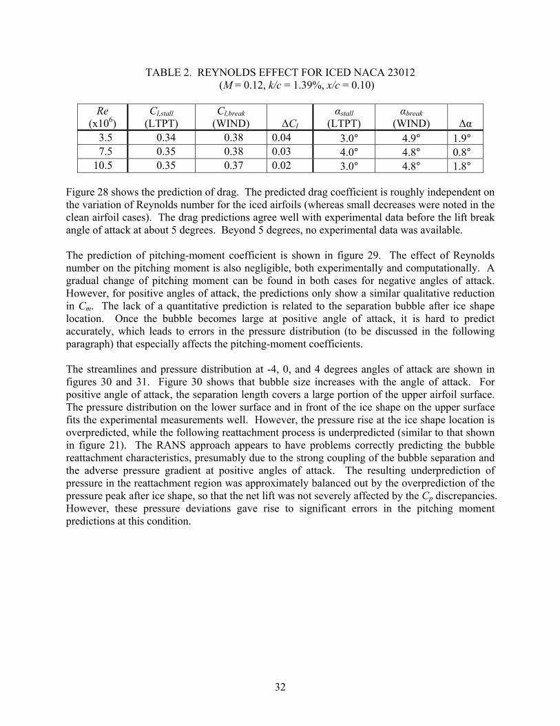
TABLE 2. REYNOLDS EFFECT FOR ICED NACA 23012 (M = 0.12, k/c = 1.39%, x/c = 0.10)

Re (x106)

Cl,stall (LTPT)

Cl,break (WIND) ∆Cl

αstall (LTPT)

αbreak (WIND) ∆α

3.5 0.34 0.38 0.04 3.0° 4.9° 1.9° 7.5 0.35 0.38 0.03 4.0° 4.8° 0.8°

10.5 0.35 0.37 0.02 3.0° 4.8° 1.8°

Figure 28 shows the prediction of drag. The predicted drag coefficient is roughly independent on the variation of Reynolds number for the iced airfoils (whereas small decreases were noted in the clean airfoil cases). The drag predictions agree well with experimental data before the lift break angle of attack at about 5 degrees. Beyond 5 degrees, no experimental data was available.

The prediction of pitching-moment coefficient is shown in figure 29. The effect of Reynolds number on the pitching moment is also negligible, both experimentally and computationally. A gradual change of pitching moment can be found in both cases for negative angles of attack. However, for positive angles of attack, the predictions only show a similar qualitative reduction in Cm. The lack of a quantitative prediction is related to the separation bubble after ice shape location. Once the bubble becomes large at positive angle of attack, it is hard to predict accurately, which leads to errors in the pressure distribution (to be discussed in the following paragraph) that especially affects the pitching-moment coefficients.

The streamlines and pressure distribution at -4, 0, and 4 degrees angles of attack are shown in figures 30 and 31. Figure 30 shows that bubble size increases with the angle of attack. For positive angle of attack, the separation length covers a large portion of the upper airfoil surface. The pressure distribution on the lower surface and in front of the ice shape on the upper surface fits the experimental measurements well. However, the pressure rise at the ice shape location is overpredicted, while the following reattachment process is underpredicted (similar to that shown in figure 21). The RANS approach appears to have problems correctly predicting the bubble reattachment characteristics, presumably due to the strong coupling of the bubble separation and the adverse pressure gradient at positive angles of attack. The resulting underprediction of pressure in the reattachment region was approximately balanced out by the overprediction of the pressure peak after ice shape, so that the net lift was not severely affected by the Cp discrepancies. However, these pressure deviations gave rise to significant errors in the pitching moment predictions at this condition.

32

(a) α = -4°

(b) α = 0°

(c) α = 4°

FIGURE 30. STREAMLINE CONFIGURATIONS FOR AN NACA 23012 AIRFOIL (k/c = 1.39%, x/c = 0.10) AT Re = 10.5x106, M = 0.12

33

-3

-2

-1

0

1

2

LTPT Data W IND-RANS

-0.2 0 0.2 0.4 0.6 0.8 1 1.2 x/c

(a) α = -4°

-3

-2

-1

0

1

2

LTPT Data W IND-RANS

-0.2 0 0.2 0.4 0.6 0.8 1 1.2 x/c

(b) α = 0°

-3

-2

-1

0

1

2-0.2 0 0.2 0.4 0.6 0.8 1 1.2

LTPT Data W IND-RANS

x/c (c) α = 4°

FIGURE 31. PRESSURE DISTRIBUTIONS FOR AN ICED NACA 23012 AIRFOIL (k/c = 1.39%, x/c = 0.10) AT Re = 10.5x106, M = 0.12

4.3 EFFECT OF MACH NUMBER FOR NACA 23012 AIRFOIL.

The effect of Mach number on airfoil aerodynamics was examined on both clean and iced NACA 23012 airfoils with the same configuration as studied above. Numerical simulations are performed at the fixed Reynolds number at 10.5x106 with three different Mach numbers (0.12, 0.21, and 0.28) corresponding to the LTPT experiment conditions.

34

C p

C pC

p

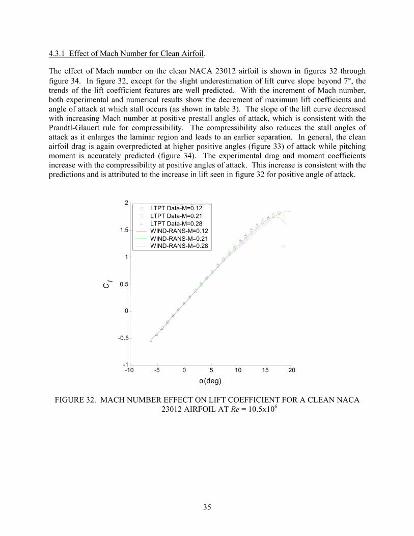
4.3.1 Effect of Mach Number for Clean Airfoil.

The effect of Mach number on the clean NACA 23012 airfoil is shown in figures 32 through figure 34. In figure 32, except for the slight underestimation of lift curve slope beyond 7°, the trends of the lift coefficient features are well predicted. With the increment of Mach number, both experimental and numerical results show the decrement of maximum lift coefficients and angle of attack at which stall occurs (as shown in table 3). The slope of the lift curve decreased with increasing Mach number at positive prestall angles of attack, which is consistent with the Prandtl-Glauert rule for compressibility. The compressibility also reduces the stall angles of attack as it enlarges the laminar region and leads to an earlier separation. In general, the clean airfoil drag is again overpredicted at higher positive angles (figure 33) of attack while pitching moment is accurately predicted (figure 34). The experimental drag and moment coefficients increase with the compressibility at positive angles of attack. This increase is consistent with the predictions and is attributed to the increase in lift seen in figure 32 for positive angle of attack.

2

1.5

1

0.5

0

-0.5

-1 -10 -5 0 5 10 15 20

LTPT Data-M=0.12 LTPT Data-M=0.21 LTPT Data-M=0.28 WIND-RANS-M=0.12 WIND-RANS-M=0.21 WIND-RANS-M=0.28

α(deg)

FIGURE 32. MACH NUMBER EFFECT ON LIFT COEFFICIENT FOR A CLEAN NACA 23012 AIRFOIL AT Re = 10.5x106

Cl

35

0.2

Cm

C

d

0.18

0.16

0.14

0.12

0.1

0.08

0.06

0.04

0.02

0

LTPT Data-M=0.12 LTPT Data-M=0.21 LTPT Data-M=0.28 WIND-RANS-M=0.12 WIND-RANS-M=0.21 WIND-RANS-M=0.28

-10 -5 0 5 10 15 20

α(deg)

FIGURE 33. MACH NUMBER EFFECT ON DRAG COEFFICIENT FOR A CLEAN NACA 23012 AIRFOIL AT Re = 10.5x106

0.15 LTPT Data-M=0.12 LTPT Data-M=0.21 LTPT Data-M=0.28

0.1 WIND-RANS-M=0.12 WIND-RANS-M=0.21 WIND-RANS-M=0.28

0.05

0

-0.05

-0.1

-10 -5 0 5 10 15 20

α(deg)

FIGURE 34. MACH NUMBER EFFECT ON PITCHING-MOMENT COEFFICIENT FOR A CLEAN NACA 23012 AIRFOIL AT Re = 10.5x106

36

TABLE 3. MACH NUMBER EFFECT FOR CLEAN NACA 23012 AT Re = 10.5x106

M Cl,stall

(LTPT) Cl,stall

(WIND) ∆Cl,stall

αstall (LTPT)

αstall (WIND) ∆αstall

0.12 1.82 1.85 0.03 17.6° 19° 1.4° 0.21 1.83 1.79 -0.04 17.6° 18° 0.4° 0.28 1.74 1.75 0.01 15.6° 17° 1.4°

4.3.2 Effect of Mach Number for Upper Surface Iced Airfoil.

Figures 35 through 37 show the compressibility effect on an iced NACA 23012 airfoil with the same ice configuration investigated in section 4.2.2. The results (experiments and predictions) show that the lift coefficients for Mach number of 0.12 are slightly greater than those for Mach number of 0.28, especially near the experimental stall (or lift-break) angle of attack. While the experimental data shows a thin-airfoil stall at 3° angle of attack, again no obvious stall is predicted in computation (as noted before in section 4.2.2). The break of the lift curve slope at around 5 degrees indicates a rapid growth of the separation bubble, and again was chosen for comparison with the experimental stall condition.

Compared to the clean airfoils, an ice shape at x/c = 0.10 makes the airfoil less sensitive to the Mach number effect since it fixes the flow separation point and renders the boundary layer development less critical, as shown in table 4. However, the Mach number effect is stronger than the Reynolds number effect for the iced case (which was also true for the clean case).

2 LTPT Data-M = 0.12 LTPT Data-M = 0.28 WIND-RANS-M = 0.12 WIND-RANS-M = 0.281.5

1

0.5

Cl

0

-0.5

-1 -10 -5 0 5 10 15 20

α(deg)

FIGURE 35. MACH NUMBER EFFECT ON LIFT COEFFICIENT FOR AN ICED NACA 23012 AIRFOIL (k/c = 1.39%, x/c = 0.10) AT Re = 10.5x106

37

0.2

0.18

0.16

0.14

0.12

0.1

0.08

0.06

0.04

0.02

0

LTPT Data-M = 0.12 LTPT Data-M = 0.28 WIND-RANS-M = 0.12 WIND-RANS-M = 0.28

Cm

C

d

-10 -5 0 5 10 15 20

α(deg)

FIGURE 36. MACH NUMBER EFFECT ON DRAG COEFFICIENT FOR AN ICED NACA 23012 AIRFOIL (k/c = 1.39%, x/c = 0.10) AT Re = 10.5x106

0.15

0.1

0.05

0

-0.05

-0.1

LTPT Data-M = 0.12 LTPT Data-M = 0.28 WIND-RANS-M = 0.12 WIND-RANS-M = 0.28

-10 -5 0 5 10 15 20

α(deg)

FIGURE 37. MACH NUMBER EFFECT ON PITCHING-MOMENT COEFFICIENT FOR AN ICED NACA 23012 AIRFOIL (k/c = 1.39%, x/c = 0.10) AT Re = 10.5x106

38

TABLE 4. MACH NUMBER EFFECT FOR ICED NACA 23012 (Re = 10.5x106, k/c = 1.39%, x/c = 0.10)

M Cl,stall

(LTPT) Cl,break

(WIND) ∆Cl,stall

αstall (LTPT)

αbreak (WIND) ∆αstall

0.12 0.35 0.37 0.02 3.0° 4.8° 1.8° 0.28 0.29 0.34 0.05 3.0° 4.4° 1.4°

Drag predictions are shown in figure 36. The compressibility effect is weak in both predictions and experiments (compared to clean airfoils), and in general, the drag is higher than in the clean case and the predictions show good agreement (actually better than in the clean case). Figure 37 shows the pitching-moment coefficient variation with angle of attack for two of the Mach numbers studied. A weak decrease in moment is found for an increasing compressibility effect, and again the experimental reduction at 0 degrees is only qualitatively predicted.

4.4 EFFECT OF ICE SHAPE SIZE FOR AIRFOILS.

The effects of ice shape size on aerodynamic performance were studied on the NACA 23012 airfoil and the NLF 0414 airfoil. The results of the upper surface quarter-round ice shape at x/c = 0.10 on the NACA 23012 and leading-edge horn ice shape at s/c = 3.4% on the NLF 0414 are shown in figures 38 through 43. The computations were conducted for the k/c = 0.83% and 1.39% upper surface ridge ice shapes and for the k/c = 2.22%, 4.44% and 6.67% leading-edge ice shapes. Reduction of the lift coefficients due to the ice shape size effect is compared with experimental data completed in the LTPT and the LSWT.

4.4.1 Upper Surface Ice Shape Size Effect for NACA 23012.

Figure 38 shows the effect of upper surface ridge ice shape size on the lift coefficient for the NACA 23012 airfoil. Computations are performed at the LTPT experimental conditions of Re = 10.5x106 and M = 0.12 for k/c = 0 and k/c = 1.39%. However, the condition for k/c = 0.83% is additionally included. The change of lift curve slope indicates that rapid changes in lift occur around 5° for k/c = 1.39% and around 6° for k/c = 0.83%. Comparing with the experimental data, for the larger ice shape (k/c = 1.39%), the significant reduction in lift curve slope and the dramatic reductions in the stall/break-lift coefficient (from about 1.8 to 0.37) and stall/break angle of attack (from about 19° to 5°) are reasonably predicted by WIND, as shown in table 5. For the smaller ice shape (k/c = 0.83%), the break-lift coefficient (0.55) was improved from the larger ice shape but still dramatically lower than the clean condition maximum lift coefficients.

Figure 39 shows the drag predictions. The trends due to the presence and height change of the ice shape are well predicted by WIND. While at lower angles of attack, both WIND and experiment predicted a small increase of drag with ice accretion, a significant increase of drag is noted at high angle of attack.

39

2 LTPT Data - Clean

1.5

1

0.5

0

-0.5

-1

LTPT Data - k/c=1.39% WIND-RANS - Clean WIND-RANS - k/c=1.39% WIND-RANS - k/c=0.83%

Cd

Cl

-10 -5 0 5 10 15 20

α(deg)

FIGURE 38. ICE SHAPE SIZE EFFECT ON LIFT COEFFICIENT FOR A NACA 23012 AIRFOIL (x/c = 0.10) AT M = 0.12, Re = 10.5x106

TABLE 5. ICE SHAPE SIZE EFFECT FOR NACA 23012 (Re = 10.5x106, k/c = 1.39%, x/c = 0.10)

k/c (%)

Cl,stall (LTPT)

Cl,break (WIND) ∆Cl,stall

αstall (LTPT)

αbreak (WIND) ∆αstall

0 1.82 1.85 0.03 17.6° 19.0° 1.4° 0.83 N/A 0.55 N/A N/A 6.2° N/A 1.39 0.35 0.37 0.02 3.0° 4.8° 1.8°

0.2

0.18

0.16

0.14

0.12

d 0.1

0.08

0.06

0.04

0.02

0

LTPT Data - Clean LTPT Data - k/c=1.39% WIND-RANS - Clean WIND-RANS - k/c=1.39% WIND-RANS - k/c=0.83%

-10 -5 0 5 10 15 20

α(deg)

FIGURE 39. ICE SHAPE SIZE EFFECT ON DRAG COEFFICIENT FOR A NACA 23012 AIRFOIL (x/c = 0.10) AT M = 0.12, Re = 10.5x106

40

Figure 40 shows pitching moment predictions. For the low angles of attack before stall, with the increment the ice shape size, the pitching-moment coefficient also increases. Near 0 degrees angle of attack for the ice shape cases, the pitching moment drops dramatically (though the effect is not quantitatively reproduced by the simulations). Note that this drop occurs significantly before the Cl,max angle of attack for the experimental case.

0.15

0.1

0.05

0

Cm

-0.05

-0.1

LTPT Data - Clean LTPT Data - k/c=1.39% WIND-RANS - Clean WIND-RANS - k/c=1.39% WIND-RANS - k/c=0.83%

-10 -5 0 5 10 15 20

α(deg)

FIGURE 40. ICE SHAPE SIZE EFFECT ON PITCHING-MOMENT COEFFICIENT FOR A NACA 23012 AIRFOIL (x/c = 0.10) AT M = 0.12, Re = 10.5x106

4.4.2 Leading-Edge Ice Shape Size Effect for NLF 0414.

The effects of leading-edge ice shape size on the NLF 0414 airfoil are shown in figures 41 through 43. A horn ice shape was attached to the NLF 0414 airfoil at a leading edge location corresponding to s/c = 3.4%, a location close to x/c = 0.02. All the cases were investigated at the LSWT experimental conditions of Re = 1.8x106 and M = 0.185.

Figure 41 shows the lift curve for the NLF 0414 with leading-edge ice shapes. With an increment of ice shape size at this location, both the stall/break angle of attack and the maximum/break-lift coefficient decrease significantly. Note that the predictions yield a Cl,max for the smallest ice shape size but only yield a break in the lift curve slope for the larger ice shapes. Therefore, the problem of predicting Cl,max noted in this case is not as severe as in figure 38, but is still significant. Considering a maximum lift coefficient of 1.35 for the clean NLF 0414, the lift degradation shown in table 6 is quite modest compared to the quarter-round ridge ice shapes. The break-lift coefficients predicted for the smallest ice shape (k/c = 2.22%) drops to 0.7 at α = 5°. Both experimental and simulation values are presented in table 6.

41

2 LSWT Data-k/c=2.22% LSWT Data-k/c=4.44% LSWT Data-k/c=6.67%

1.5 WIND-RANS-k/c=2.22% WIND-RANS-k/c=4.44% WIND-RANS-k/c=6.67%

1

0.5

0

-0.5

-1 -10 -5 0 5 10 15 20

α(deg)

FIGURE 41. ICE SHAPE SIZE EFFECT ON LIFT COEFFICIENT FOR AN NLF 0414 AIRFOIL (s/c = 3.4%) AT M = 0.185, Re = 10.8x106

TABLE 6. ICE SHAPE SIZE EFFECT FOR NLF 0414 (Re = 10.8x106, M = 0.185, s/c = 3.4%)

Cd

Cl

k/c (%)

Cl,stall (LTPT)

Cl,break (WIND) ∆Cl,stall

αstall (LTPT)

αbreak (WIND) ∆αstall

2.22 0.72 0.71 -0.01 5.1° 5.4° 0.3° 4.44 0.56 0.55 -0.01 3.1° 2.9° -0.2° 6.67 0.43 0.44 -0.01 1.1° 1.1° 0.0°

Figure 42 shows the drag prediction for various ice shape height sizes at the leading edge location s/c = 3.4%. At lower angles of attack (<-5°), the difference for the drag with different ice shape sizes is generally not as significant as that at larger angles of attack, where larger ice shapes consistently lead to increases of drag coefficient. As in the upper surface ice shape conditions, the drag predictions match quite well with experiments.

0.2

0.18

0.16

0.14

0.12

0.1

0.08

0.06

LSWT Data-k/c=2.22% LSWT Data-k/c=4.44% LSWT Data-k/c=6.67% W IND-RANS-k/c=2.22% W IND-RANS-k/c=4.44%

0.04

0.02 WIND-RANS-k/c=6.67%

0 -10 -5 0 5 10 15 20

α(deg)

FIGURE 42. ICE SHAPE SIZE EFFECT ON DRAG COEFFICIENT FOR AN NLF 0414 AIRFOIL (s/c = 3.4%) AT M = 0.185, Re = 10.8x106

42

Figure 43 shows the pitching-moment coefficients variation with angle of attack for the NLF 0414 airfoil with leading-edge ice shapes. The predictions indicate that a higher pitching moment is associated with a larger ice shape at the lower angles of attack (<0°). The largest pitching moment is also found a few degrees in advance of stall/break angle of attack. The trends are more representative of the experimental results compared to the case for the upper surface ice shapes of the NACA 23012 airfoil (figure 40).

0.15

0.1

0.05

0

LSW T Data-k/c=2.22% LSW T Data-k/c=4.44% LSW T Data-k/c=6.67% WIND-RANS-k/c=2.22% WIND-RANS-k/c=4.44% WIND-RANS-k/c=6.67%

Cm

-0.05

-0.1

-10 -5 0 5 10 15 20 α(deg)

FIGURE 43. ICE SHAPE SIZE EFFECT ON PITCHING-MOMENT COEFFICIENT FOR AN NLF 0414 AIRFOIL (s/c = 3.4%) AT M = 0.185, Re = 10.8x106

4.5 EFFECT OF WING VS AIRFOIL.

Since real flight conditions involve wings (of finite aspect ratio), it was important to consider whether the airfoil trends are similar to those for typical wing configurations. Therefore, a few 3-D numerical simulations were also performed to examine the relationship to corresponding 2-D (airfoil) computations. A wing was studied under a typical LTPT Mach number of 0.12. A Reynolds number of 10.5x106 at the root chord was specified, where a k/c = 1.39% quarter-round ice shape was located at x/c = 0.10. The simulated wing has an aspect ratio of 5 and taper ratio of 2 (such that the tip chord Reynolds number was 5.25x106). To keep the ice shape size parameter k/c fixed over the entire span, the simulated ice shape size was also tapered from the root plane to the tip. The main wing surface grid is shown in figure 44.

43

FIGURE 44. SURFACE GRID PROFILE OF ICED NACA 23012 WING

Figure 45 shows the lift curve for the iced wing and its comparison to the airfoil results. As expected, a slightly lower lift curve slope is predicted for the wing compared with the airfoil due to finite wing losses. The prediction also shows stall may be slightly delayed for the wing because the lift curve break was at about 4 degrees for the airfoil and 5 degrees for the wing. Also, it is noted that the effect of three-dimensionality produced a stronger break in the lift curve slope, nearly yielding a Clmax. Figure 46 shows the drag predictions for the 3-D wing. The simulated drag coefficient and curve slope for the wing is slightly lower than that of the airfoils, but, in general, the dimensionality had little effect on the drag. This is because the large increase in drag due to the ice shape presence overshadows the increase in induced drag for a finite aspect ratio.

1

0.8

0.6

0.4

0.2

0

-0.2

-0.4

-0.6 -10 -5 0 5 10 15 20

α(deg)

WIND-Airfoil WIND-Wing

Cl

FIGURE 45. LIFT COEFFICIENT FOR THE ICED NACA 23012 AIRFOIL AND WING (k/c = 1.39%, x/c = 0.10) AT M = 0.12, Re = 10.5x106

44

0.35

0.3

0.25

0.2

WIND-Airfoil WIND-Wing

Cd

0.15

0.1

0.05

0-10 -5 0 5 10 15 20

α(deg)

FIGURE 46. DRAG COEFFICIENT FOR THE ICED NACA 23012 AIRFOIL AND WING (k/c = 1.39%, x/c = 0.10) AT M = 0.12, Re = 10.5x106

5. CRITICAL ICE SHAPE METHODOLOGY.

The favorable airfoil aerodynamics is mainly attributed to its streamlined body shape. When ice accretes on the airfoil‘s surface, its shape is modified and its aerodynamic properties are changed, generally degraded. With the ice shape located at different positions, the effect on airfoil body shape profile and aerodynamics can vary significantly. At a critical ice shape location, the most deteriorated aerodynamics is obtained for a given ice shape size. To examine the ice shape location effect and find the critical ice shape location, simulations were performed for the NACA 23012 airfoil and wing and other airfoil models with the ice shape at different leading edge and upper surface locations under the LTPT/LSWT experimental conditions. The results are compared to experimental data when available.

5.1 EFFECT OF ICE SHAPE LOCATION FOR ICED NACA 23012 AIRFOIL.

The effect of ice shapes on the lift coefficient due to various ice shape locations was studied on a clean NACA 23012 airfoil with both leading-edge and upper surface ice shape configurations. A horn ice shape with a larger k/c = 4.4% was attached at different leading edge locations to be representative of glaze ice shape configurations (as shown in figure 47); and a quarter-round ice shape with k/c = 1.39% was attached at different upper surface locations as representative of the 2-D ridge ice shape configurations (as shown in figure 48). Simulations were performed at the LTPT condition of Re = 10.5x106 and M = 0.12 to be comparable to LTPT experimental results.

45

(a) x/c = 0.00%

(b) x/c = 0.095%

(c) x/c = 1.9%

FIGURE 47. LEADING-EDGE ICE SHAPE CONFIGURATIONS ON A NACA 23012 AIRFOIL WITH k/c = 4.44% ICE SHAPE AT DIFFERENT

LEADING EDGE LOCATIONS

(a) x/c = 0.02

(b) x/c = 0.10

(c) x/c = 0.20

FIGURE 48. UPPER SURFACE ICE SHAPE CONFIGURATIONS ON A NACA 23012 AIRFOIL WITH k/c = 1.39% ICE SHAPE AT DIFFERENT

UPPER SURFACE LOCATIONS

Figures 49 and 50 show the lift prediction for the two ice shape configurations. In figure 49, the k/c = 4.44% horn ice shapes were studied at three leading edge locations: x/c = 0.00%, 0.95%, and 1.9%. As seen before, there is a less severe reduction (from the clean case) of the lift curve slope and maximum lift coefficient for the ice shapes at the immediate leading edge location x/c = 0.00. In particular, the maximum lift coefficient reduced from 1.79 in the clean case to 1.08 and the predictions show a definite maximum lift coefficient (not just a break) at this location, though the drop-off is not as mild as was found experimentally. However, for the ice shape at x/c = 0.95%, the break-lift coefficient drops significantly from 1.08 to 0.54. For the ice shape at x/c = 1.9%, the penalty is more severe as the Cl,break drops to a lower value of 0.38.

46

The decrease of the stall (break) angles of attack and the stall (break) lift coefficients as the ice shape moves aft is seen to be significant for both the predictions and the experiments. For the range considered herein, 1.9% of chord is the most critical ice shape location. In addition, the predicted results were important in identifying that the lift from the pressure taps may be neglecting a significant force on the ice shape itself. The use of the force balance data showed a result more consistent with the predictions. This is one of the few times that the predictions helped in the interpretation of the experimental data.

2

1.5

1

0.5

0

-0.5

-1

LTPT Data-x/c=0.00(Bal) LTPT Data-x/c=0.019(Bal) WIND-RANS-x/c=0.00 WIND-RANS-x/c=0.019 WIND-RANS-x/c=0.0095

-10 -5 0 5 10 15 20

α(deg)

FIGURE 49. ICE SHAPE LOCATION EFFECT ON LIFT COEFFICIENT FOR THE LEADING-EDGE ICED NACA 23012 AIRFOIL (k/c = 4.44%) AT

M = 0.12, Re = 10.5x106

Cl

Cl

2

1.5

1

0.5

0

-0.5

-1

LTPT Data-Clean LTPT Data-x/c=0.02 LTPT Data-x/c=0.10 LTPT Data-x/c=0.20 WIND-RANS-Clean WIND-RANS-x/c=0.02 WIND-RANS-x/c=0.10 WIND-RANS-x/c=0.20

-10 -5 0 5 10 15 20

α(deg)

FIGURE 50. ICE SHAPE LOCATION EFFECT ON LIFT COEFFICIENT FOR THE UPPER SURFACE ICED NACA 23012 AIRFOIL (k/c = 1.39%) AT

M = 0.12, Re = 10.5x106

47

Figure 50 shows the lift for a k/c = 1.39% quarter-round ice shape at three upper surface positions of x/c = 0.02, 0.10 and 0.20. A thin-airfoil stall was predicted in x/c = 0.02 case with lift coefficient at 0.53, which is larger than the previous horn ice shape lift at almost the same location (x/c = 0.019) with a value of 0.39. Considering a larger ice shape involved in the leading edge case, the larger prediction of lift is reasonable. Unlike what was shown in experimental results, there are no obvious stalls existing in the two downstream location ice shape cases‘ predictions. A lift break for the x/c = 0.10 case was predicted at about angle of attack of 5 degrees, but the x/c = 0.20 case did not exhibit a strong enough change in Clα to allow determination of Cl,break. The largest reduction in the break lift is for the x/c = 0.10 case. Considering that it is larger than the x/c = 0.02 case (which was approximately shown to be the most critical location of the leading-edge shapes) and x/c = 0.20 case, the x/c = 0.10 is the critical ice shape location for NACA 23012 airfoil. The corresponding break-lift coefficient is 0.37 at α = 4.8°. This prediction is roughly compatible with the experimental stall condition. The qualitative values of lift prediction are shown in tables 7 and 8.

TABLE 7. ICE SHAPE LOCATION (LEADING-EDGE) EFFECT FOR NACA 23012 (Re = 10.5x106, M = 0.12, k/c = 4.44%)

x/c (%)

Cl,stall (LTPT)

Cl,break (WIND) ∆Cl

αstall (LTPT)

αbreak (WIND) ∆α

0 0.92 1.08 0.16 11.1° 10.0° -1.1° 0.95 N/A 0.49 N/A N/A 5.0° N/A 1.9 0.42 0.39 -0.03 4.0° 4.4° -0.4°

TABLE 8. ICE SHAPE LOCATION (UPPER SURFACE) EFFECT FOR NACA 23012 (Re = 10.5x106, M = 0.12, k/c = 1.39%)

x/c Cl,stall

(LTPT) Cl,break

(WIND) ∆Cl

αstall (LTPT)

αbreak (WIND) ∆α

0.02 0.59 0.53 -0.06 6.1° 6.0° -0.1° 0.10 0.35 0.37 -0.01 3.0° 4.8° 0.0° 0.20 0.52 N/A N/A 7.1° N/A N/A

The drag predictions are shown in figures 51 and 52. For the leading-edge ice shapes, the drag increased with the ice shape location moving downstream from x/c = 0.0% to x/c = 1.9% for the positive angles of attack. For the upper surface ice shape cases, the largest drag was predicted for x/c = 0.10 cases at the positive angles of attack. This greater drag prediction for ice shape at x/c = 0.10 again demonstrates that the most deteriorated aerodynamics takes place with the ice shape at this location once a fixed size is considered. Again, the numerical predictions fit the experimental data reasonably well.

48

0.18

0.2 LTPT Data-x/c=0.00(Bal) LTPT Data-x/c=0.019(Bal) WIND-RANS-x/c=0.00 WIND-RANS-x/c=0.019 WIND-RANS-x/c=0.0095 0.16

0.14

0.12

Cd

Cd 0.1

0.08

0.06

0.04

0.02

0 -10 -5 0 5 10 15 20

α(deg)

FIGURE 51. ICE SHAPE LOCATION EFFECT ON DRAG COEFFICIENT FOR THE LEADING-EDGE ICED NACA 23012 AIRFOIL (k/c = 4.44%) AT M = 0.12,

Re = 10.5x106

0.2

0.18

0.16

0.14

0.12

0.1

0.08

LTPT Data-Clean LTPT Data-x/c=0.02 LTPT Data-x/c=0.10 LTPT Data-x/c=0.20 WIND-RANS-Clean WIND-RANS-x/c=0.02 WIND-RANS-x/c=0.10 WIND-RANS-x/c=0.20

0.06

0.04

0.02

0 -10 -5 0 5 10 15 20

α(deg)

FIGURE 52. ICE SHAPE LOCATION EFFECT ON DRAG COEFFICIENT FOR THE UPPER SURFACE ICED NACA 23012 AIRFOIL (k/c = 1.39%) AT M = 0.12,

Re = 10.5x106

Figures 53 and 54 show the pitching moment predictions. For the leading-edge ice shape cases (figure 53) with negative angle of attack, the pitching moment increases as the ice shape is located more downstream. At positive angles of attack, the drop-off is exacerbated as the ice location move aft to 1.9%. For the upper surface ice shape cases (figure 54), the moment coefficients are very similar at lower incidences. The location x/c = 0.10 for the ice shape

49

location yields the most rapid drop-off of the pitching moment, which is consistent with its poor lift and drag performance. This confirms (experimentally and computationally) that this is the critical ice shape location.

0.15

0.1

0.05

0

-0.05

-0.1

LTPT Data-x/c=0.00(Bal) LTPT Data-x/c=0.019(Bal) WIND-RANS-x/c=0.00 WIND-RANS-x/c=0.019 WIND-RANS-x/c=0.0095

-10 -5 0 5 10 15 20

α(deg)

FIGURE 53. ICE SHAPE LOCATION EFFECT ON PITCHING-MOMENT COEFFICIENT FOR THE LEADING-EDGE ICED NACA 23012 AIRFOIL (k/c = 4.44%)

AT M = 0.12, Re = 10.5x106

0.15

0.1

0.05

0

-0.05

-0.1

LTPT Data-Clean LTPT Data-x/c=0.02 LTPT Data-x/c=0.10 LTPT Data-x/c=0.20 WIND-RANS-Clean WIND-RANS-x/c=0.02 WIND-RANS-x/c=0.10 WIND-RANS-x/c=0.20

-10 -5 0 5 10 15 20

α(deg)

FIGURE 54. ICE SHAPE LOCATION EFFECT ON PICHING-MOMENT COEFFICIENT FOR THE UPPER SURFACE ICED NACA 23012 AIRFOIL (k/c = 1.39%) AT

M = 0.12, Re = 10.5x106

Cm

Cm

50

The pressure distributions at 0 degree angle of attack for upper surface ice shape cases are shown in figure 55. As seen before, the pressure is well predicted for the lower surface and upper surface in front of the ice shape. After the ice shape, the bubble region is not well captured, especially for the x/c = 0.10 simulation case. However, both the experiments and predictions show that the x/c = 0.1 case has the largest discontinuous pressure coefficient change over the ice shape, where there is a change of nearly two (Cp drops from 0.6 to -1.3). The representative streamline profiles were shown in figure 56. Interestingly, the separation bubble for x/c = 0.20 is similar to or even larger than that for x/c = 0.10. This indicates that bubble separation length is not necessarily a robust predictor of critical ice shape location (although clearly the x/c = 0.02 location yields a much smaller separation bubble).

-3

-2

-1

0

1

2

LTPT Data WIND-RANS

-0.2 0 0.2 0.4 0.6 0.8 1 1.2

x/c (a) x/c = 0.02

-3

-2

-1

0

1

2

LTPT Data WIND-RANS

-0.2 0 0.2 0.4 0.6 0.8 1 1.2

x/c (b) x/c = 0.10

-3

-2

-1

0

1

2

LTPT Data WIND-RANS

-0.2 0 0.2 0.4 0.6 0.8 1 1.2

x/c (c) x/c = 0.20

Cp

Cp

Cp

FIGURE 55. PRESSURE DISTRIBUTIONS FOR THE UPPER SURFACE ICED NACA 23012 AIRFOIL AT α = 0°, M = 0.12, Re = 10.5x106

51

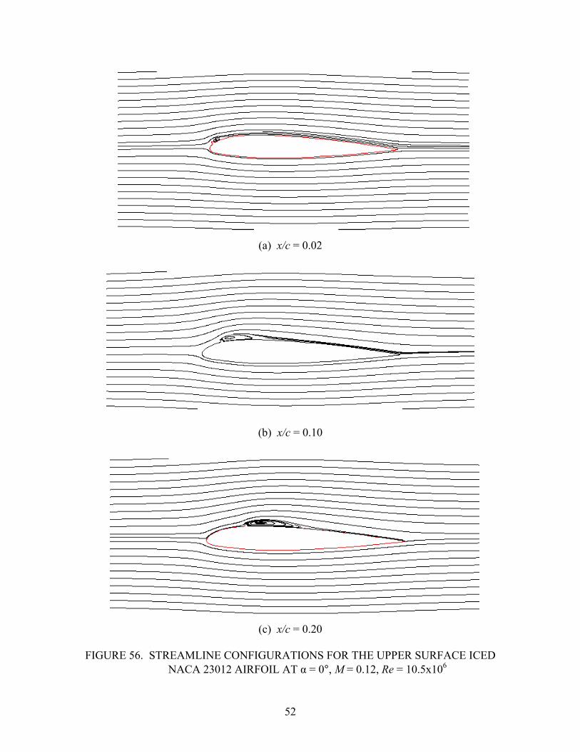
(a) x/c = 0.02

(b) x/c = 0.10

(c) x/c = 0.20

FIGURE 56. STREAMLINE CONFIGURATIONS FOR THE UPPER SURFACE ICED NACA 23012 AIRFOIL AT α = 0°, M = 0.12, Re = 10.5x106

52

5.2 EFFECT OF ICE SHAPE LOCATION ON OTHER AIRFOILS.

The effect on the lift coefficients due to variation in airfoil geometries was also studied for four other airfoils: NACA 3415, NLF 0414, Large Transportation Horizontal Stabilizer model (LTHS), and BJMW. In their iced configuration cases, each included the same chordwise forward quarter-round ice shape (k/c = 1.39%) attached at various upper surface locations. The geometries of these four airfoils and NACA 23012 airfoil are shown in figure 57. The five airfoils can be divided into two categories, where the NACA 23012 (tmax/c = 12.07%), NLF 0414 (tmax/c = 14.32%), and NACA 3415 (tmax/c = 15.18%) airfoils are much thicker than the other LTHS (tmax/c = 8.97%) and BJMW (tmax/c = 8.67%) airfoils. For the first three airfoils, simulations were conducted at both Re = 1.8x106 and Re = 10.5x106. Herein, the lower Reynolds number results for NLF 0414 and NACA 3415 to allow comparison with LSWT experimental data are shown. However, the predictions were effectively independent of Reynolds and Mach numbers. For the latter two airfoils (LTHS and BJMW), only the Re = 10.5x106 condition is presented in order to be consistent with the LTPT conditions and typical flight conditions.

NACA23012

Y

X-0.2 0 0.2 0.4 0.6 0.8 1 1.2-0.1

-0.05

0

0.05

0.1 NLF0414 NACA3415 LTHS BJMW

FIGURE 57. GEOMETRY PROFILES FOR THE FIVE AIRFOILS STUDIED

Figures 58 through 61 show the lift coefficients curves for the each airfoil in the clean status and with ice shapes attached. As shown in figures 58 and 59, the lift slope and Cl,max for the clean NACA 3415 and NLF 0414 were overpredicted for the positive angle of attack, especially for NLF 0414 airfoil. This is attributed to the difficulty in the precise prediction of complicated transition processes involved in these two more aft-loaded airfoils (a finding consistent with other clean computational fluid dynamics predictions for these type of airfoils in their clean configuration). However, the lift coefficients are reasonably predicted up to the stall angle of attack for all the iced configurations with the NACA 3415 airfoil. In particular, the critical ice shape location for this airfoil was found at x/c = 0.20 with a break-lift angle of attack at 4.5 degrees with a break-lift value of 0.43 (table 9). For the NLF 0414 airfoil, the critical ice shape moves downstream further at x/c = 0.30 with a break-lift angle at about 3 degrees. This prediction is compatible with UIUC experimental study as shown in table 10. In general, the lift is much less sensitive to x/c location for the NLF 0414 airfoil compared to that of NACA 3415 airfoil. In figures 60 and 61, the LTHS and BJMW airfoils were found to have a much more upstream critical ice shape location because x/c = 0.02 was found to yield the most deteriorated aerodynamics (also shown in tables 11 and table 12).

53

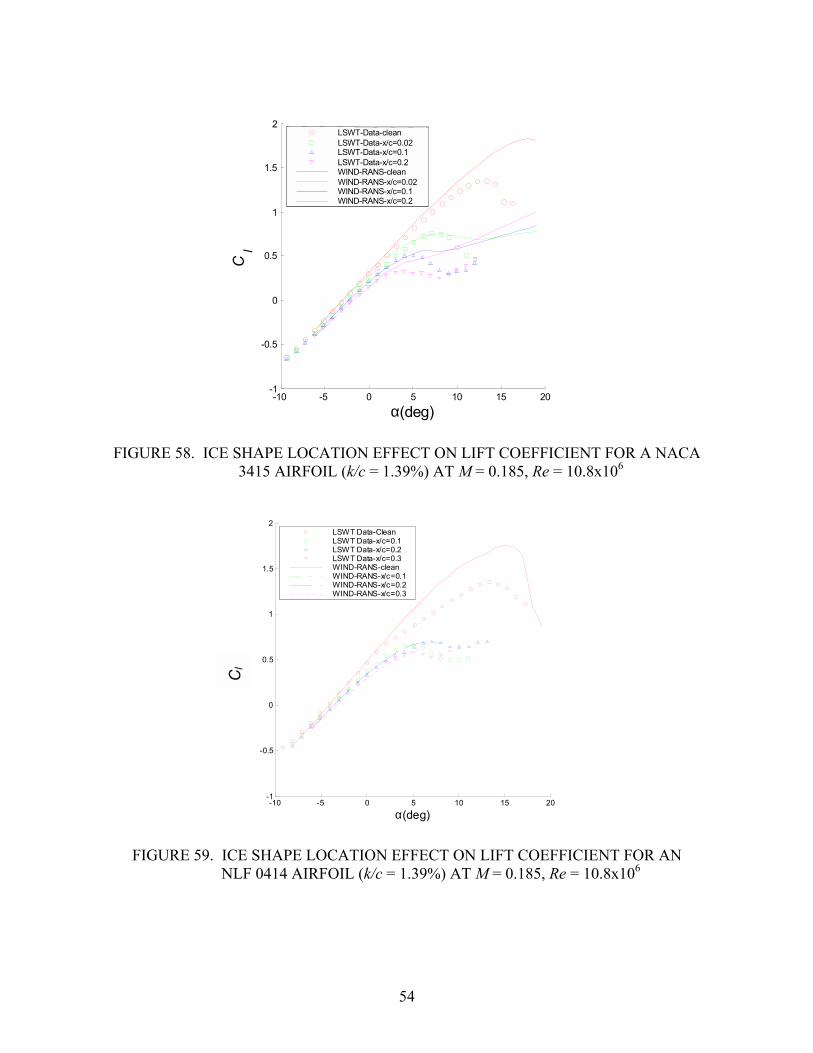
2

1.5

1

0.5

0

-0.5

-1 -10 -5 0 5 10 15 20

LSWT-Data-clean LSWT-Data-x/c=0.02 LSWT-Data-x/c=0.1 LSWT-Data-x/c=0.2 WIND-RANS-clean WIND-RANS-x/c=0.02 WIND-RANS-x/c=0.1 WIND-RANS-x/c=0.2

α(deg)

FIGURE 58. ICE SHAPE LOCATION EFFECT ON LIFT COEFFICIENT FOR A NACA 3415 AIRFOIL (k/c = 1.39%) AT M = 0.185, Re = 10.8x106

2 LSWT Data-Clean LSW T Data-x/c=0.1 LSW T Data-x/c=0.2 LSW T Data-x/c=0.3 WIND-RANS-clean WIND-RANS-x/c=0.1 WIND-RANS-x/c=0.2 WIND-RANS-x/c=0.3

1.5

1

0.5

0

-0.5

-1 -10 -5 0 5 10 15 20

α(deg)

FIGURE 59. ICE SHAPE LOCATION EFFECT ON LIFT COEFFICIENT FOR AN NLF 0414 AIRFOIL (k/c = 1.39%) AT M = 0.185, Re = 10.8x106

Cl

Cl

54

2 WIND-Clean WIND-x/c=0.02 WIND-x/c=0.10

1.5 WIND-x/c=0.20

1

0.5

0

-0.5

-1 -10 -5 0 5 10 15 20

α(deg)

FIGURE 60. ICE SHAPE LOCATION EFFECT ON LIFT COEFFICIENT FOR AN LTHS AIRFOIL (k/c = 1.39%) AT M = 0.12, Re = 10.5x106

2 WIND-Clean WIND-x/c=0.02 WIND-x/c=0.10

1.5 WIND-x/c=0.20

1

0.5

0

-0.5

-1 -10 -5 0 5 10 15 20

α(deg)

FIGURE 61. ICE SHAPE LOCATION EFFECT ON LIFT COEFFICIENT FOR A BJMW AIRFOIL (k/c = 1.39%) AT M = 0.12, Re = 10.5x106

Cl

Cl

55

TABLE 9. ICE SHAPE LOCATION EFFECT FOR NACA 3415 (Re = 10.8x106, M = 0.12, k/c = 1.39%)

x/c Cl,stall

(LTPT) Cl,break

(WIND) ∆Cl

αstall (LTPT)

αbreak (WIND) ∆α

0.02 0.76 0.75 -0.01 7.2° 8.0° -0.8° 0.10 0.50 0.51 0.01 5.0° 4.8° -0.2° 0.20 0.32 0.43 0.11 4.0° 4.5° 0.5°

TABLE 10. ICE SHAPE LOCATION EFFECT FOR NLF 0414 (Re = 10.8x106, M = 0.12, k/c = 1.39%)

x/c Cl,stall

(LTPT) Cl,break

(WIND) ∆Cl

αstall (LTPT)

αbreak (WIND) ∆α

0.10 0.66 0.68 0.02 4.1° 6.0° 1.9° 0.20 0.70 0.69 -0.01 7.1° 6.0° -1.1° 0.30 0.58 0.51 -0.07 5.0° 3.4° -1.6°

TABLE 11. ICE SHAPE LOCATION EFFECT FOR LTHS (Re = 10.5x106, M = 0.12, k/c = 1.39%)

x/c Cl,stall

(LTPT) Cl,break

(WIND) ∆Cl

αstall (LTPT)

αbreak (WIND) ∆α

0.02 N/A 0.48 N/A N/A 5.8° N/A 0.10 N/A 0.82 N/A N/A 10° N/A 0.20 N/A 0.78 N/A N/A 10° N/A

TABLE 12. ICE SHAPE LOCATION EFFECT FOR BJMW (Re = 10.5x106, M = 0.12, k/c = 1.39%)

x/c Cl,stall

(LTPT) Cl,break

(WIND) ∆Cl

αstall (LTPT)

αbreak (WIND) ∆α

0.02 N/A 0.82 N/A NA 10.0° N/A 0.10 N/A 0.95 N/A NA 12.0° N/A 0.20 N/A 0.95 N/A NA 12.0° N/A

Figures 62 through 65 show the drag predictions. Associated with a lower lift value for airfoils with ice shapes at the critical location, higher drags are measured and predicted for those conditions. Comparing with the UIUC experimental data for the NACA 3415 and NLF 0414 airfoils, the WIND simulations gave good predictions of the drag value and trends for ice shape location. Again the NLF 0414 airfoil shows the least sensitivity to ice shape location, whereas the most sensitive airfoil is the NACA 23012. Note that the LTHS is more sensitive to x/c location than the BJMW, which is attributed to a lower minimum Cp for the latter (a similar difference occurs between the NLF 0414 and the NACA 23012 airfoils).

56

0.2

0.18

0.16

0.14

0.12

0.1

0.08

0.06

0.04

0.02

LSWT-Data-clean LSWT-Data-x/c=0.02 LSWT-Data-x/c=0.1 LSWT-Data-x/c=0.2 WIND-RANS-clean WIND-RANS-x/c=0.02 WIND-RANS-x/c=0.1 WIND-RANS-x/c=0.2

0 -10 -5 0 5 10 15 20

α(deg)

FIGURE 62. ICE SHAPE LOCATION EFFECT ON DRAG COEFFICIENT FOR A NACA 3415 AIRFOIL (k/c = 1.39%) AT M = 0.185, Re = 10.5x106

0.2

0.18

LSW T Data-Clean LSW T Data-x/c=0.1 LSW T Data-x/c=0.2 LSW T Data-x/c=0.3 WIND-RANS-clean WIND-RANS-x/c=0.1 WIND-RANS-x/c=0.2 WIND-RANS-x/c=0.3

0.16

0.14

0.12

0.1

0.08

0.06

0.04

0.02

0 -10 -5 0 5 10 15 20

α(deg)

Cd

Cd

FIGURE 63. ICE SHAPE LOCATION EFFECT ON DRAG COEFFICIENT FOR AN NLF 0414 AIRFOIL (k/c = 1.39%) AT M = 0.185, Re = 10.8x106

57

0.2

0.18

WIND-Clean WIND-x/c=0.02 WIND-x/c=0.10 WIND-x/c=0.20

0.16

0.14

0.12

0.1

0.08

0.06

0.04

0.02

0-10 -5 0 5 10 15 20

α(deg)

FIGURE 64. ICE SHAPE LOCATION EFFECT ON DRAG COEFFICIENT FOR AN LTHS AIRFOIL (k/c = 1.39%) AT M = 0.12, Re = 10.5x106

0.2 WIND-Clean WIND-x/c=0.02 WIND-x/c=0.10 WIND-x/c=0.20

0.18

0.16

0.14

0.12

0.1

0.08

0.06

0.04

0.02

0-10 -5 0 5 10 15 20

α(deg)

FIGURE 65. ICE SHAPE LOCATION EFFECT ON DRAG COEFFICIENT FOR A BJMW AIRFOIL (k/c = 1.39%) AT M = 0.12, Re = 10.5x106

Figures 66 through 69 show the moment coefficients at different angles of attack with ice shapes at different locations. For the NACA 3415 airfoil with ice shapes at locations of x/c = 0.02 and 0.10, the simulation results fit well with the experimental data. With the ice shape moving forward to x/c = 0.20, which is the critical ice shape location, the moment is somewhat overpredicted after the break. This is similar to results for the NACA 23012 airfoil. Similar discrepancies in the moment are also shown in figure 67 for NLF 0414 airfoil, indicating that the

Cd

Cd

58

poorest prediction is typically at the critical ice shape location. However, the qualitative trend of the moment decreasing (nose down) with the ice shape moving downstream is still reasonably predicted. For the LTHS airfoil, the moment for the iced airfoil with ice shapes at x/c = 0.02 was not necessarily found to yield the largest drop-off. For the BJMW airfoil with ice shapes at x/c = 0.02 and x/c = 0.10, the predicted moment again does not yield the greatest drop-off at the critical ice shape location, which is at x/c = 0.02. Thus, the thinner airfoils tend to have only drag and lift degradation highly correlated with the critical ice shape location, whereas the thicker airfoils showed correlation with lift, drag, and pitching moment. This is attributed to the different types of stall patterns between the two groups.

0.15 LSWT-Data-clean LSWT-Data-x/c=0.02 LSWT-Data-x/c=0.1

0.1 LSWT-Data-x/c=0.2 WIND-RANS-clean WIND-RANS-x/c=0.02 WIND-RANS-x/c=0.10.05 WIND-RANS-x/c=0.2

0

-0.05

-0.1

-10 -5 0 5 10 15 20 α(deg)

FIGURE 66. ICE SHAPE LOCATION EFFECT ON PITCHING-MOMENT COEFFICIENT FOR A NACA 3415 AIRFOIL (k/c = 1.39%) AT M = 0.185, Re = 10.8x106

0.15 LSWT Data-Clean LSWT Data-x/c=0.1 LSWT Data-x/c=0.2

0.1LSWT Data-x/c=0.3 WIND-RANS-clean WIND-RANS-x/c=0.1 WIND-RANS-x/c=0.2 WIND-RANS-x/c=0.3

0.05

0

-0.05

-0.1

-10 -5 0 5 10 15 20 α(deg)

Cm

Cm

FIGURE 67. ICE SHAPE LOCATION EFFECT ON PITCHING-MOMENT COEFFICIENT FOR AN NLF 0414 AIRFOIL (k/c = 1.39%) AT M = 0.185, Re = 10.8x106

59

0.15 WIND-Clean WIND-x/c=0.02 WIND-x/c=0.10

0.1 WIND-x/c=0.20

0.05

0

-0.05

-0.1

-10 -5 0 5 10 15 20

α(deg)

FIGURE 68. ICE SHAPE LOCATION EFFECT ON PITCHING-MOMENT COEFFICIENT FOR AN LTHS AIRFOIL (k/c = 1.39%) AT M = 0.12, Re = 10.5x106

0.15 WIND-Clean WIND-x/c=0.02 WIND-x/c=0.10

0.1 WIND-x/c=0.20

0.05

0

-0.05

-0.1

-10 -5 0 5 10 15 20

α(deg)

FIGURE 69. ICE SHAPE LOCATION EFFECT ON PITCHING-MOMENT COEFFICIENT FOR A BJMW AIRFOIL (k/c = 1.39%) AT M = 0.185, Re = 10.8x106

The relation between the predicted break-lift coefficients and the ice shape locations for different airfoils is shown in figure 70. In the five airfoils studied, the NACA 23012, NACA 3415 and NLF 0414 airfoils yielded the most deteriorated aerodynamic performance when ice shapes were located at 10%, 20%, and 30% of chord length respectively. The two other airfoils, LTHS and BJMW, have a more forward critical ice shape location at 2% (or perhaps further forward) of chord length. Thus, the thicker airfoils were more sensitive to upper surface ice, while thinner airfoils were more sensitive to leading-edge ice.

Cm

Cm

60

1.2

1.1

1

0.9

0.8

0.7

0.6

0.5

0.4

0.3 0 0.05 0.1 0.15 0.2 0.25

WIND-NACA23012 WIND-NLF0414 WIND-NACA3415 WIND-LTHS WIND-BJMW

x/c

FIGURE 70. ICE SHAPE LOCATION EFFECT ON BREAK-LIFT COEFFICIENT FOR THE ICED AIRFOILS

The significantly different aerodynamic responses to the ice shapes for those airfoils are thought to be related to the different aerodynamic load patterns for the clean models. Figure 71 shows the pressure distribution for these five clean airfoil models with the same lift value of 0.5. The suction peaks of the two thinner airfoils, the LTHS and the BJMW, are quite close to the leading edge. For the NACA 23012 airfoil, the suction peak is located at around 7% of the chord length. For the NACA 3415 airfoil, it is at about 18% of chord length. There is no obvious suction peak for NLF 0414 airfoil, instead it includes a flat plateau from the leading edge (x/c = 2%) to the 60% chord location. The relation between the critical ice shape and the pressure load pattern for different airfoil models is shown in table 13. With the selected Cl value of 0.5, the critical ice shape location is generally between the locations of Cp,min (pressure suction peak) and (dCp/dx)min (peak adverse pressure gradient). The correlation with Cp,min can be explained as that of an ice shape located at the suction peak will lead to a reduction of that peak and, thus, of the net lift. The correlation with (dCp/dx)min can be explained as follows. The bubble size will be longer when the ice shape is located in the region of the most adverse pressure gradient, and a larger separation bubble will more strongly degrade the airfoil aerodynamic performance.

With the largest Cp,min among the thick airfoils, the NACA 23012 airfoil yields the most deteriorated aerodynamic performance with a 80% lift reduction for the critical ice shape location. The least affected thick airfoil, the NLF 0414, still has a 70% lift reduction. Among the thin airfoils, the performance degradation is not as significant and, in particular, the BJMW airfoil is the least affected and also has a less severe Cp spike compared to the LTHS airfoil. The thinner airfoils may not provide as much maximum clean airfoil lift as the thicker airfoils do, but they tend to show better resistance to the aerodynamic degradation stemming from ice shapes of a fixed size.

Cl,

brea

k

61

Cp

-5

-4

-3

-2

-1

0

1

2

WIND-NACA23012 WIND-NLF0414 WIND-NACA3415 WIND-LTHS WIND-BJMW

-0.2 0 0.2 0.4 0.6 0.8 1 1.2

x/c

FIGURE 71. PRESSURE DISTRIBUTIONS FOR THE CLEAN AIRFOILS AT Cl = 0.5

TABLE 13. RELATION BETWEEN CRITICAL ICE SHAPE LOCATION AND SPECIAL SURFACE PRESSURE LOCATIONS (Re = 10.5x106, M = 0.12, k/c = 1.39%)

Airfoil (x/c) Cp,min (x/c) crit (x/c)(dCp/dx),min (Cl,break)crit (Cl,stall)clean ∆Cl, ∆Cl (%) LTHS 0.33% ~2% 0.35% 0.38 0.84 0.46 54.76% BJMW 0.49% ~2% 0.51% 0.82 1.11 0.29 26.13%

NACA 23012 6.99% ~10% 15% 0.34 1.79 1.45 81.01% NACA 3415 17.49% ~20% 39% 0.42 1.82 1.46 80.22% NLF 0414 2%-60% ~30% 73% 0.50 1.68 1.18 70.24%

5.3 EFFECT OF ICE SHAPE LOCATION ON ICED NACA 23012 WING.

As all the above simulations were conducted for airfoils (2-D), a wing (3-D) study was also performed to investigate whether the effect of ice shape location was different. Because of its significant requirements for computer resources, this study was conducted only for an iced NACA 23012 wing with ice shapes located at x/c = 0.2, 0.10, and 0.20. As in section 4.5, the wing aspect ratio is 5.0 and taper ratio is 2 with M = 0.12 and Re = 10.5x106 (where Re was based on root chord), similar to that of the baseline LTPT experimental condition.

Figure 72 shows the surface grid for 3-D NACA 23012 wing with an ice shape located at x/c = 0.2. In the spanwise direction, the grid points were clustered at the tip because of the rapid spanwise gradients in section aerodynamics near this position. To be compatible with the 2-D airfoil study, the ice shape height was kept at a consistent ratio to the local chord, i.e., (k/c)local = 1.39%.

62

FIGURE 72. SURFACE GRID FOR ICED NACA 23012 WING WITH k/c = 1.39%, x/c = 0.02

Figure 73 shows the lift curve for the clean and iced wings. As was the case in the 2-D simulations, no obvious Cl,max and αstall were predicted for the wings with ice shape at x/c = 0.10 and 0.20, though the x/c = 0.02 did yield a maximum lift coefficient. Again, the maximum Cl changes were obtained when the ice shape location was at x/c = 0.10, the same critical ice shape location found in the airfoil study. This is reasonable considering that the wing has a NACA 23012 airfoil section along its entire span. The detailed values are shown in table 14. For the x/c = 0.02 and 0.1 cases, the differences are small between the airfoil and wing predictions. At x/c = 0.20, the lift curve slope does not undergo a strong enough change to determine a Cl,break for either the airfoil or the wing case, so a quantitative comparison cannot be made, but the curve shapes are qualitatively similar, which is the same results as for the airfoil (figure 50). Thus, the critical ice shape location for the wing is the same for the airfoil case.

2

1.5

1

0.5

0

-0.5

-1 -10 -5 0 5 10 15 20

WIND-Wing-clean WIND-Wing-x/c=0.02 WIND-Wing-x/c=0.10 WIND-Wing-x/c=0.20

α(deg)

Cl

FIGURE 73. ICE SHAPE LOCATION EFFECT ON LIFT COEFFICIENT FOR A NACA 23012 WING (k/c = 1.39%) AT M = 0.12, Re = 10.5x106

63

TABLE 14. ICE SHAPE LOCATION EFFECT FOR NACA 23012 (Re = 10.5x106, M = 0.12, k/c = 1.39%)

x/c Cl,break

(WIND-airfoil) Cl,break

(WIND-wing) ∆Cl

αbreak (WIND-airfoil)

αbreak (WIND-wing) ∆α

0.02 0.53 0.60 0.07 6.0° 8.0° 2° 0.10 0.37 0.34 -0.04 4.8° 5.0° 0.2° 0.20 N/A N/A N/A N/A N/A N/A

Figure 74 shows the drag predictions at different angles of attack for the wing. The result was similar to the drag profile predicted with the airfoil in figure 52 (although there is a noticeable difference for the clean condition, which is attributed to the addition of induced drag). Therefore, the overall effect of ice shape location on an iced wing was similar to that on the iced airfoils.

Cd

0.2

0.18

0.16

0.14

0.12

0.1

0.08

0.06

0.04

0.02

0

WIND-Wing-clean WIND-Wing-x/c=0.02 WIND-Wing-x/c=0.10 WIND-Wing-x/c=0.20

-10 -5 0 5 10 15 20 α(deg)

FIGURE 74. ICE SHAPE LOCATION EFFECT ON DRAG COEFFICIENT FOR A NACA 23012 WING (k/c = 1.39%) AT M = 0.12, Re = 10.5x106

6. SUMMARY, CONCLUSIONS, AND RECOMMENDATIONS.

6.1 SUMMARY.

The Reynolds-Averaged Navier Stokes (RANS) approach was applied in this study to investigate the ice shape effect on airfoil and wing aerodynamics under diverse conditions. Effects of Reynolds and Mach numbers as well as ice shape size and location and inclusion of a finite aspect ratio on the aerodynamic performance were studied for several clean and iced airfoil and wing models. Compared with the experimental results, steady RANS simulations predict the main aerodynamic trends reasonably well up to (but not typically beyond) the stall condition. Specific conclusions are given in the following.

64

6.2 CONCLUSIONS.

The grid sensitivity, turbulence model effect, and three-dimensional (3-D) capability aspects of WIND were assessed through detailed validations of selected clean and iced airfoil and wing cases. Results were compared with Low Turbulence Pressure Tunnel experimental data or previously reported simulation and experimental results. Of the various turbulence models considered, the Mentor-Shear Stress Transport model and especially the Spalart-Allmaras models gave the best overall performance, and the latter was chosen for all the performance simulations. However, it should be noted that the choice of the turbulence model yielded large variations in the results and that no single model was entirely robust. In general, a grid of 400 x 100 points in the chordwise and normalwise directions was found to be suitable for grid independence and, thus, was used for all the airfoil performance simulations. For the wing simulations, a somewhat coarser grid of 208 x 61 was used combined with 48 points in the spanwise direction (26 along the wing and 22 beyond the wing tip). To evaluate the possible influence of the grid topology (motivated by differences noted between the unstructured grid NSU2D results and the structured grid WIND results), the FLUENT code was employed because it allows for both structured and unstructured grids with a common numerical discretization scheme. The results indicated that the differences between the structured and unstructured grids were small when both grids were suitably refined. For the clean conditions, there were very small differences between the results for various numerical approaches, whereas the upper surface iced condition yielded the largest variations between numerical schemes and also between computations and experiments. In particular, significant variations were found for changes in the scheme, e.g., use of first- versus second-order scheme and use of segregated versus coupled schemes. The WIND second-order upwind scheme tended to yield the best results for lift predictions (though not necessarily pressure predictions) for the upper surface iced airfoils and, thus, was chosen as the numerical scheme for use in the performance studies.

For clean airfoils, the effect of increasing Reynolds number (for fixed Mach number) was to slightly increase the maximum lift coefficient, lift curve slope, and pitching moment as well as to slightly decrease the drag coefficient. The WIND methodology was able to consistently predict these trends. However, it exhibited variations from the experimental data (especially for the drag coefficient), which were on the order of trend variations. For upper surface iced airfoils, the variations between Reynolds numbers were effectively negligible for both the experimental and computational results. However, it was noted that the WIND code did not generally predict a maximum lift coefficient (as noted in the experiments) and instead only predicted a substantial break in the lift curve slope. In addition, the rapid pitching moment drop-off found in the experiments was noted to a lesser degree and at a later angle for the simulations. The latter results indicate an inability of the WIND code to correctly predict the pressure distribution at higher angles of attack. This was confirmed with analysis of the Cp plots, whereby the separated flow region was generally underpredicted in extent and overpredicted with respect to initial pressure rise behind the ice shape. The lack of a true maximum lift coefficient and the overprediction of the separation bubble length were observed in the results from FLUENT and NSU2D as well as WIND; furthermore, they were observed for all the turbulence models investigated, and for the wing as well as the airfoil simulations. Therefore, the inability to accurately predict Cl,max and the poststall behavior is attributed to the RANS formalism (and not the particular capabilities of WIND, FLUENT, or NSU2D). However, on a positive note, it is

65

significant that the break values of Cl and α reasonably match most of the experimental Cl,max and αstall values.

For the clean airfoil predictions, increasing Mach number reduced the angle of attack at which stall occurred (and hence reduced the maximum lift coefficient) and also yielded larger drag and pitching-moment coefficients. In general, the Mach number sensitivity (over the range of 0.12 to 0.28) was greater than that found for the Reynolds number effects (over the range of 3.5x106 to 10.5x106) and was consistent with the experimental trends. Compared with clean airfoils, the airfoils with upper surface ice shapes are more resistant to the effects of Mach number, which is attributed to the fact the ice shape forces the flow separation to take place just aft of the ice shape location for all conditions.

Effects of ice shape size on the lift, drag, and pitching-moment coefficients for the NACA 23012 and NLF 0414 airfoils with upper surface quarter-round ridge heights of 0.83% and 1.39% are dramatic. For the NACA 23012 airfoil, the k/c = 0.83% ice shape at x/c = 0.10 significantly reduces the break-lift coefficient from 1.85 to 0.55, whereas the k/c = 1.39% ice shape at the same location yields a break-lift coefficient of 0.37. Notably, a nearly two-fold increase in height does not lead to a commensurate reduction in lift coefficient, i.e., the change is nonlinear with respect to ice shape size. This is consistent with the experimental findings for the upper surface ice shapes. For the leading-edge iced NLF 0414 airfoil, the size effect at the leading edge (x/c = 0.00) is still significant but not as large and in general, the variations in lift, drag, and pitching moment tend to vary more linearly with ice shape size.

Effects of location of ice shape were especially studied to assess the critical ice shape position. For the NACA 23012 airfoil with a fixed ice shape size, the maximum lift coefficient and stall angle of attack are worse at the critical ice shape location of x/c = 0.10. A similar result was noted for a NACA 23012 wing. However, it should be noted that the reduction in the break-lift coefficient at an x/c of 1.9% with a k/c of 4.44% is similar to the reduction at an x/c of 10% (the critical ice shape location) for a k/c of 1.39%. This is important, since larger ice shape heights tend to be found (in accretion studies) near the leading edge compared to along the upper surface. Thus, considering the critical position for a fixed ice shape may not be representative of the typical icing scenarios.

The study for ice accretions on different airfoil models shows that the critical ice location varies with airfoil model, and in general, the location tends to be nearby (often between) the positions of the maximum pressure gradient and the minimum pressure of the clean airfoil condition. This result is consistent with available experimental data. In general, the thick airfoils tended to have the largest performance degradation and had critical ice shape locations that corresponded to upper surface positions. In contrast, the thin airfoils (which had pressure peaks close to the leading edge) tended to be more insensitive to lift degradation (for the same ice shape size) but yielded critical ice shape locations near the leading edge. For the thick airfoils, an increase in the suction peak for a given lift coefficient for the clean airfoil condition generally corresponded to performance degradation under iced conditions. In particular, the NACA23012 yielded the biggest lift losses followed by the NACA3415 airfoil and then by the relatively well-performing NLF0414 airfoil. This overall trend was consistent with experimental observations. Similarly, among the thin airfoils, the Large Transportation Horizontal Stabilizer airfoil yielded larger

66

reductions in the break-lift coefficient and had a higher clean airfoil suction peak compared to the Business Jet Main Wing model.

6.3 RECOMMENDATIONS.

Additional simulations are needed to more fully understand the details of Mach number, ice shape size, and ice shape location effects for airfoils other than the NACA 23012. Additional simulations with wing geometries for some of the above parametric studies would be of importance, since only a few such studies have been conducted, thus limiting the general interpretation of airfoil results to wing conditions. In particular, wing simulations for airfoils other than the NACA 23012 would be of interest.

While the RANS method shows reasonable prediction of the clean airfoil performance and of the iced airfoil aerodynamics before stall, the stall or poststall prediction of the flow field generally involves unsteady 3-D massively separated flows. This regime (necessary to predict the maximum lift coefficient) is generally beyond the capability of current RANS methodologies for iced airfoil conditions (particularly for large ice shapes and for upper surface ice shapes). Thus, to obtain a more robust computational capability of iced airfoil aerodynamics, unsteady 3-D full (versus thin layer) Navier-Stokes simulation methodologies (such as detached eddy simulations or large eddy simulations) should be considered.

7. REFERENCES.

1. Johnson, C.L., —Wing Loading, Icing and Associated Aspects of Modern Transport Design,“ Journal of the Aeronautical Sciences, Vol. 8, No. 2, pp. 43-54, December 1940.

2. Thoren R.L., —Icing Flight Tests on the Lockheed P2V,“ ASME Paper No. 48-SA-41, 1948.

3. Bragg M.B., —Aircraft Aerodynamic Effects Due To large Droplet Ice Accretion,“ AIAA Paper 96-0932, January 1996.

4. Lee, S. and Bragg, M.B., —Effects of Simulated-Spanwise Ice Shapes on Airfoils: Experimental Investigation,“ AIAA Paper 99-0092, January 1999.

5. Lee, S., Kim, H.S., and Bragg, M.B., —Investigation of Factors that Influence Iced-Airfoil Aerodynamics,“ AIAA Paper 2000-0099, January 2000.

6. Kim, H.S. and Bragg, M.B., —Effect of Leading-Edge Ice Accretion Geometry on Airfoil Aerodynamics,“ AIAA Paper 99-3150, January 2001.

7. Bragg, M.B. and Loth, E., —Effects of Large-Droplet Ice Accretion on Airfoil and Wing Aerodynamics and Control,“ FAA Report, DOT/FAA/AR-00/14, April 2000.

8. Dunn T., —Prediction of Iced-Airfoil Aerodynamics,“ Master Thesis, October 1998.

67

9. Potapczuk, M. —Numerical Analysis of a NACA0012 Airfoil with Leading Edge Ice Accretions,“ AIAA Paper 87-0101, January 1987.

10. Caruso, S.C., —Development of an Unstructured Mesh/Navier-Stokes Method for Aerodynamics of Aircraft with Ice Accretions,“ AIAA Paper 90-0758, January 1990.

11. Caruso, S.C. and Farshchi, M., —Automatic Grid Generation for Iced Airfoil Flowfield Predictions,“ AIAA Paper 92-0415, January 1992.

12. Dompierre, J., Cronin, D.J., Bourgault, Y., Baruzzi, G.S., Habashi, G., and Wagner, A., —Numerical Simulation of Performance Degradation of Ice Contaminated Airfoils,“ AIAA Paper 97-2235, 1997.

13. Dunn, T. and Loth, E., —Effects of Simulated-Spanwise-Ice Shapes on Airfoils: Computational Investigation,“ AIAA Paper 99-0093, January 1999.

14. Kumar, S. and Loth, E., —Aerodynamic Simulations of Airfoils with Large-Droplet Ice shapes,“ 38th Aerospace Sciences Meeting and Exhibit, Reno NV, AIAA 00-0238, 2000.

15. Kwon, O. and Sankar, O., —Numerical Study of the Effects of Icing on Finite Wing Aerodynamics,“ AIAA Paper 92-0757, January 1990.

16. Kwon, O. and Sankar, O., —Numerical Study of the Effects of Icing on Fixed and Rotary Wing Performance,“ AIAA Paper 91-0662, January 1991.

17. Bragg, M.B. and Khodadoust A., —Effect of Simulated Glaze Ice on a Rectangular Wing,“ AIAA Paper 89-0750, January 1989.

18. Chung J., Choo, Y., Reehorst, A., Potapczuk, M., and Slater, J., —Navier-Stokes Analysis of the Flowfield Characteristics of an Ice Contaminated Aircraft Wing,“ 37th AIAA Aerospace Sciences Meeting and Exhibit, AIAA Paper 99-0375, 1999.

19. Bush, R.H., Power, G.D., and Towne, C.E., —WIND: The Production Flow Solver of the NPARC Alliance,“ AIAA Paper 98-0935, January 1998.

20. —FLUENT 6.0 User‘s Guide,“ Fluent Inc., November 2001.

21. Mavriplis, D., —A CFD Package for Multi-Element Airfoil High-Lift Analysis (Revision 4),“ Scientific Simulations, December 1996.

22. Spalart, P.R. and Allmaras, S.R., —A One-Equation Turbulence Model for Aerodynamic Flows,“ AIAA Paper 92-0439, January 1992.

23. Bardina, J.E., Huang, P.G., and Coakley, T.J., —Turbulence Modeling Validation, Testing, and Development,“ NASA TM-110446, April 1997.

68

24. Drela, M. and Giles, M.B., —Viscous-Inviscid Analysis of Transonic and Low Reynolds Number Airfoils,“ AIAA Journal, Vol. 25, No. 10, pp.1347-1355, October 1987.

25. —XFOIL 6.94 User Primer,“ MIT Aero and Astro Engineering, December 6, 2001.

26. Drela, M. and Giles, M.B., —A Two-Dimensional Viscous Aerodynamic Design and Analysis Code,“ AIAA Paper 87-0424, January 1987.

27. Broeren, A., Lee, S., LaMarre, C and Bragg, M.B., —Effect of Airfoil Geometry on Performance With Simulated Ice Accretions, Volume 1: Experimental Investigation,“ FAA Report, DOT/FAA/AR-03/64, August 2003.

69/70