1

EFFECT OF A TEMPERATURE CYCLE ON A ROTATING ELASTIC-PLASTICSHAFT

A THESIS SUBMITTED TOTHE GRADUATE SCHOOL OF NATURAL AND APPLIED SCIENCES

OFMIDDLE EAST TECHNICAL UNIVERSITY

BY

ERAY ARSLAN

IN PARTIAL FULFILLMENT OF THE REQUIREMENTSFOR

THE DEGREE OF DOCTOR OF PHILOSOPHYIN

ENGINEERING SCIENCES

JANUARY 2010

Approval of the thesis:

EFFECT OF A TEMPERATURE CYCLE ON A ROTATING

ELASTIC-PLASTIC SHAFT

submitted by ERAY ARSLAN in partial fulfillment of the requirements for the degreeof Doctor of Philosophy in Engineering Sciences Department, Middle EastTechnical University by,

Prof. Dr. Canan OzgenDean, Graduate School of Natural and Applied Sciences

Prof. Dr. Turgut TokdemirHead of Department, Engineering Sciences

Prof. Dr. Ahmet N. EraslanSupervisor, Engineering Sciences Department, METU

Examining Committee Members:

Prof. Dr. Tulay OzbelgeChemical Engineering Dept., METU

Prof. Dr. Ahmet N. EraslanEngineering Sciences Dept., METU

Prof. Dr. M. Polat SakaEngineering Sciences Dept., METU

Assoc. Prof. Dr. Zafer EvisEngineering Sciences Dept., METU

Asst. Prof. Dr. A. Hakan ArgesoManufacturing Engineering Dept., Atılım University

Date: January 28, 2010

I hereby declare that all information in this document has been obtainedand presented in accordance with academic rules and ethical conduct. Ialso declare that, as required by these rules and conduct, I have fully citedand referenced all material and results that are not original to this work.

Name, Last Name: ERAY ARSLAN

Signature :

iii

ABSTRACT

EFFECT OF A TEMPERATURE CYCLE ON A ROTATING ELASTIC-PLASTICSHAFT

Arslan, Eray

Ph.D., Department of Engineering Sciences

Supervisor : Prof. Dr. Ahmet N. Eraslan

January 2010, 161 pages

The stress distribution in a rotating solid shaft with temperature dependent yield

stress subject to a temperature cycle is investigated. It is presumed that the shaft

is in a state of generalized plane strain and obeys Tresca’s yield criterion and the

flow rule associated with it. By the temperature cycle it is meant that the surface

temperature of the shaft is increased to a limiting value, it is held at this temperature

for a while, and then slowly decreased at the same rate to the reference temperature.

The isothermal shaft is rotated up to around elastic limit rotation speed and then

the temperature cycle is applied to the surface of the shaft. Even in an initially

purely elastic shaft, two plastic regions with different forms of the yield condition

emerge simultaneously at the centre and expand into the elastic region. However, the

expansion of the plastic zone ceases soon thereafter, and an unloaded region spreads

into the plastic core. It is shown that the stress distribution is altered significantly by

the temperature cycle, hence also leading to non-zero residual stresses at stand-still.

Keywords: Rotating shaft, temperature cycle, elastoplasticity, Tresca’s criterion

iv

OZ

SICAKLIK CEVRIMININ DONEN ELASTIK-PLASTIK MIL UZERINDEKIETKISI

Arslan, Eray

Doktora, Muhendislik Bilimleri Bolumu

Tez Yoneticisi : Prof. Dr. Ahmet N. Eraslan

Ocak 2010, 161 sayfa

Sıcaklık cevrimi uygulanan, sıcaklıga baglı akma gerilmesine sahip malzemeden yapılmıs

donen bir mildeki gerilim dagılımı incelenmistir. Duzlem sekil degistirme kosulu ve mil

malzemesinin Tresca akma kriteri ve ilgili akma kuralına uygun oldugu varsayılmaktadır.

Sıcaklık cevrimi, milin yuzey sıcaklıgının bir limit degerine kadar artırılması, bu

sıcaklıkta bir sure tutulması ve referans sıcaklıgına aynı oranda azaltılması olarak

tanımlanmıstır. Izotermal mil elastik limit donme hızı civarına kadar dondurulmekte

ve daha sonra milin dıs yuzeyine sıcaklık cevrimi uygulanmaktadır. Bu durumda,

baslangıcta tamamiyle elastik davranan milin merkezinde farklı akma kosullarına sahip

iki plastik bolge aynı anda ortaya cıkmakta ve bu plastik bolgeler elastik bolgeye

dogru genislemektedir. Fakat bir sure sonra plastik bolgenin genislemesi sona ermekte

ve bosaltma bolgesi (unloading region) plastik merkeze dogru yayılmaktadır. Sonuc

olarak mildeki gerilim dagılımı, sıcaklık cevrimiyle onemli olcude degismekte ve bu da

milde artık gerilmelerin (residual stresses) olusmasına sebep olmaktadır.

Anahtar Kelimeler: Donen mil, sıcaklık cevrimi, elastoplastisite, Tresca akma kriteri

v

To My Family and Prof. Werner Mack

vi

ACKNOWLEDGMENTS

I wish to express my deepest gratitude to my advisor Prof. Dr. Ahmet N. Eraslan

and Prof. Dr. Werner Mack (Vienna University of Technology, Austria) for their

guidance, advice, criticism, and insight throughout this study.

I am also indebted to Prof. Dr. Udo Gamer (Vienna University of Technology, Aus-

tria) for many helpful discussions.

I owe special thanks to my advisory committee members Prof. Dr. M. Polat Saka

and Prof. Dr. Tulay Ozbelge and examining committee members Assoc. Prof. Dr.

Zafer Evis and Asst. Prof. Dr. A. Hakan Argeso for their remarkable suggestions and

comments.

I would also like to thank Prof. Dr. M. Rusen Gecit for his helpful advices and

guidance.

I wish to extend my thanks to my roommate Baran Aydın for his useful discussions

and friendship, and to Academic Writing Center of METU for their collaborative effort

at the grammatical supervision of the study.

Finally, the biggest thanks go to my parents, my brothers and the most special person

in my life Pelin Yuksel for their endless love, patience, support and encouragement.

This study was financially supported by the State Planning Organization (DPT) Grant

No: BAP-08-11-DPT2002K120510.

vii

TABLE OF CONTENTS

ABSTRACT . . . . . . . . . . . . . . . . . . . . . . . . . . . . . . . . . . . . . iv

OZ . . . . . . . . . . . . . . . . . . . . . . . . . . . . . . . . . . . . . . . . . . . v

DEDICATON . . . . . . . . . . . . . . . . . . . . . . . . . . . . . . . . . . . . . vi

ACKNOWLEDGMENTS . . . . . . . . . . . . . . . . . . . . . . . . . . . . . . vii

TABLE OF CONTENTS . . . . . . . . . . . . . . . . . . . . . . . . . . . . . . viii

LIST OF TABLES . . . . . . . . . . . . . . . . . . . . . . . . . . . . . . . . . . xi

LIST OF FIGURES . . . . . . . . . . . . . . . . . . . . . . . . . . . . . . . . . xii

CHAPTERS

1 INTRODUCTION . . . . . . . . . . . . . . . . . . . . . . . . . . . . . 1

1.1 General Aspects . . . . . . . . . . . . . . . . . . . . . . . . . . 1

1.2 Related Literature . . . . . . . . . . . . . . . . . . . . . . . . . 1

1.2.1 Rotating Cylindrical Elements without Thermal Load-ing . . . . . . . . . . . . . . . . . . . . . . . . . . . . 2

1.2.2 Cylindrical Elements under Thermal Load . . . . . . 4

1.2.3 Rotating Cylindrical Elements under Thermal Load . 6

1.3 Scope of the Present Work . . . . . . . . . . . . . . . . . . . . 7

2 THEORY . . . . . . . . . . . . . . . . . . . . . . . . . . . . . . . . . . 9

2.1 The Stress-Strain Relation . . . . . . . . . . . . . . . . . . . . 9

2.2 Criteria of Yielding . . . . . . . . . . . . . . . . . . . . . . . . 11

2.2.1 Von Mises’ Yield Criterion . . . . . . . . . . . . . . . 11

2.2.2 Tresca’s Yield Criterion . . . . . . . . . . . . . . . . 11

2.3 Flow Rule Associated with Yield Criteria . . . . . . . . . . . . 13

2.3.1 Flow Rule Associated with Tresca Yield Function . . 15

viii

3 STATEMENT OF THE PROBLEM AND TEMPERATURE FIELD . 17

3.1 Statement of the Problem . . . . . . . . . . . . . . . . . . . . . 17

3.2 Temperature Field . . . . . . . . . . . . . . . . . . . . . . . . . 18

4 BASIC EQUATIONS AND ANALYTICAL SOLUTIONS OF ELAS-TIC AND PLASTIC REGIONS . . . . . . . . . . . . . . . . . . . . . 22

4.1 Basic Equations . . . . . . . . . . . . . . . . . . . . . . . . . . 22

4.2 Elastic Region . . . . . . . . . . . . . . . . . . . . . . . . . . . 23

4.3 Plastic (Edge Regime) Region I . . . . . . . . . . . . . . . . . 26

4.4 Plastic (Side Regime) Region II . . . . . . . . . . . . . . . . . 29

4.5 Predeformed Elastic Region . . . . . . . . . . . . . . . . . . . 34

5 EVOLUTION OF STRESSES DURING TEMPERATURE CYCLE . 37

5.1 Purely Elastic State . . . . . . . . . . . . . . . . . . . . . . . . 37

5.2 Elastic-Plastic State . . . . . . . . . . . . . . . . . . . . . . . . 38

5.3 Unloaded State . . . . . . . . . . . . . . . . . . . . . . . . . . 40

6 RESULTS AND DISCUSSION . . . . . . . . . . . . . . . . . . . . . . 43

6.1 Non-Dimensional and Normalized Quantities . . . . . . . . . . 43

6.2 Numerical Results . . . . . . . . . . . . . . . . . . . . . . . . . 44

6.3 Summary and Discussion . . . . . . . . . . . . . . . . . . . . . 111

7 CONCLUSION . . . . . . . . . . . . . . . . . . . . . . . . . . . . . . . 113

REFERENCES . . . . . . . . . . . . . . . . . . . . . . . . . . . . . . . . . . . . 114

APPENDICES

A DESCRIPTION OF FORTRAN CODES . . . . . . . . . . . . . . . . 119

B FORTRAN CODES OF PURELY ELASTIC STATE . . . . . . . . . 123

B.1 MAIN PROGRAM: PURELY ELASTIC STATE . . . . . . . 123

B.2 SUBROUTINE: TEMPERATURE DISTRIBUTION . . . . . 126

B.3 FUNCTION: TEMPERATURE . . . . . . . . . . . . . . . . . 128

B.4 FUNCTION: TEMPERATURE INTEGRAL 1 . . . . . . . . . 129

B.5 FUNCTION: SERIES 1 . . . . . . . . . . . . . . . . . . . . . . 130

B.6 FUNCTION: SERIES 2 . . . . . . . . . . . . . . . . . . . . . . 132

ix

x

C FORTRAN CODES OF ELASTIC-PLASTIC STATE . . . . . . . . . . . . . 134

C.1 MAIN PROGRAM: ELASTIC-PLASTIC STATE . . . . . . . . . . 134

C.2 SUBROUTINE: NLNEQN . . . . . . . . . . . . . . . . . . . . . . . . . . 140

C.3 SUBROUTINE: PLASTIC REGION I . . . . . . . . . . . . . . . . . . 144

C.4 SUBROUTINE: PLASTIC REGION II. . . . . . . . . . . . . . . . . . 145

C.5 SUBROUTINE: ELASTIC REGION . . . . . . . . . . . . . . . . . . . 147

C.6 FUNCTION: TEMPERATURE INTEGRAL 2 . . . . . . . . . . . . 149

C.7 FUNCTION: SERIES 3 . . . . . . . . . . . . . . . . . . . . . . . . . . . . 150

C.8 FUNCTION: HYPERGEOMETRIC FUNCTION . . . . . . . . . . 152

D FORTRAN CODES OF UNLOADED STATE . . . . . . . . . . . . . . . . . . 154

D.1 MAIN PROGRAM: UNLOADED STATE . . . . . . . . . . . . . . . 154

D.2 DATA FILE: PERMANENT PLASTIC STRAINS . . . . . . . . . . 159

VITA . . . . . . . . . . . . . . . . . . . . . . . . . . . . . . . . . . . . . . . . . . . . . . . . . . . 162

LIST OF TABLES

TABLES

Table 6.1 Calculated constants of C2 and ε0 at different rotations speeds in

purely elastic state . . . . . . . . . . . . . . . . . . . . . . . . . . . . . . . 46

Table 6.2 Calculated constants of C2 and ε0 versus time in purely elastic state 58

Table 6.3 Calculated constants in elastic-plastic state at different time values . 67

Table 6.4 Calculated constants in unloaded state at different time values until

the end of the temperature cycle . . . . . . . . . . . . . . . . . . . . . . . . 86

Table 6.5 Calculated constants in unloaded state at different time values after

the temperature cycle . . . . . . . . . . . . . . . . . . . . . . . . . . . . . 87

Table 6.6 Differences in response variables between the beginning and the end

of the thermal process . . . . . . . . . . . . . . . . . . . . . . . . . . . . . 100

Table D.1 Permanent plastic strains at τ ≥ 1.7882 . . . . . . . . . . . . . . . . 159

xi

LIST OF FIGURES

FIGURES

Figure 1.1 Categories of the studies in the literature . . . . . . . . . . . . . . . 2

Figure 2.1 Stress-strain Diagram . . . . . . . . . . . . . . . . . . . . . . . . . . 10

Figure 2.2 Tresca’s hexagon with yielding conditions on three-dimensional prin-

cipal stress space . . . . . . . . . . . . . . . . . . . . . . . . . . . . . . . . 12

Figure 3.1 Sketch of the rotating solid shaft subjected to temperature cycle . . 18

Figure 3.2 Prescribed surface temperature of the shaft . . . . . . . . . . . . . 19

Figure 3.3 Description of surface temperature with linear function . . . . . . . 20

Figure 6.1 Prescribed surface temperature of the shaft (x = 1) . . . . . . . . . 45

Figure 6.2 Transient temperature field at τ ≤ 1.2 . . . . . . . . . . . . . . . . 47

Figure 6.3 Transient temperature field at 1.2 ≤ τ ≤ 1.5 . . . . . . . . . . . . . 48

Figure 6.4 Transient temperature field at 1.5 ≤ τ ≤ 2.7 . . . . . . . . . . . . . 49

Figure 6.5 Transient temperature field at 2.7 ≤ τ ≤ 3.0 . . . . . . . . . . . . . 50

Figure 6.6 Transient temperature field at 3.0 ≤ τ ≤ 3.6 . . . . . . . . . . . . . 51

Figure 6.7 Change of temperature difference between outer surface and the

center of the shaft with time . . . . . . . . . . . . . . . . . . . . . . . . . . 52

Figure 6.8 Radial stress distribution in the shaft with increasing rotation speed 53

Figure 6.9 Circumferential stress distribution in the shaft with increasing rota-

tion speed . . . . . . . . . . . . . . . . . . . . . . . . . . . . . . . . . . . . 54

Figure 6.10 Axial stress distribution in the shaft with increasing rotation speed 55

Figure 6.11 Radial displacement distribution in the shaft with increasing rotation

speed . . . . . . . . . . . . . . . . . . . . . . . . . . . . . . . . . . . . . . . 56

xii

Figure 6.12 Stresses and radial displacement distributions in purely elastic state

under Ω = 0.9× Ωie = 1.5875 . . . . . . . . . . . . . . . . . . . . . . . . . . 57

Figure 6.13 Ratio of equivalent and yield stresses at different time until plastic

flow . . . . . . . . . . . . . . . . . . . . . . . . . . . . . . . . . . . . . . . . 59

Figure 6.14 Change of ratio of equivalent and yield stresses with time until plastic

flow at the center . . . . . . . . . . . . . . . . . . . . . . . . . . . . . . . . 60

Figure 6.15 Radial stress distribution at different time steps in purely elastic state 61

Figure 6.16 Circumferential stress distribution at different time steps in purely

elastic state . . . . . . . . . . . . . . . . . . . . . . . . . . . . . . . . . . . 62

Figure 6.17 Axial stress distribution at different time steps in purely elastic state 63

Figure 6.18 Radial displacement distribution at different time steps in purely

elastic state . . . . . . . . . . . . . . . . . . . . . . . . . . . . . . . . . . . 64

Figure 6.19 Stresses and radial displacement distributions in purely elastic state

at τ = τp = 1.5519 . . . . . . . . . . . . . . . . . . . . . . . . . . . . . . . . 65

Figure 6.20 Evolutions of plastic tangential strain component with time at x = 0

and x = x1 . . . . . . . . . . . . . . . . . . . . . . . . . . . . . . . . . . . . 69

Figure 6.21 Evolutions of derivative of plastic tangential strain with time at

x = 0 and x = x1 . . . . . . . . . . . . . . . . . . . . . . . . . . . . . . . . 70

Figure 6.22 Evolution of interface radius x2 with time . . . . . . . . . . . . . . 71

Figure 6.23 Evolution of derivative of x2 with respect to time . . . . . . . . . . 72

Figure 6.24 Stresses and radial displacement distributions in elastic-plastic state

at τ = τp = 1.5519 . . . . . . . . . . . . . . . . . . . . . . . . . . . . . . . . 73

Figure 6.25 Stresses and radial displacement distributions in elastic-plastic state

at τ = 1.57 . . . . . . . . . . . . . . . . . . . . . . . . . . . . . . . . . . . . 74

Figure 6.26 Stresses and radial displacement distributions in elastic-plastic state

at τ = 1.6 . . . . . . . . . . . . . . . . . . . . . . . . . . . . . . . . . . . . 75

Figure 6.27 Stresses and radial displacement distributions in elastic-plastic state

at τ = 1.66 . . . . . . . . . . . . . . . . . . . . . . . . . . . . . . . . . . . . 76

Figure 6.28 Stresses and radial displacement distributions in elastic-plastic state

at τ = 1.72 . . . . . . . . . . . . . . . . . . . . . . . . . . . . . . . . . . . . 77

xiii

Figure 6.29 Stresses and radial displacement distributions in elastic-plastic state

at τ = τub = 1.7882 . . . . . . . . . . . . . . . . . . . . . . . . . . . . . . . 78

Figure 6.30 Plastic strain distributions in elastic-plastic state at τ = 1.57 . . . . 79

Figure 6.31 Plastic strain distributions in elastic-plastic state at τ = 1.6 . . . . 80

Figure 6.32 Plastic strain distributions in elastic-plastic state at τ = 1.66 . . . . 81

Figure 6.33 Plastic strain distributions in elastic-plastic state at τ = 1.72 . . . . 82

Figure 6.34 Plastic strain distributions in elastic-plastic state at τ = τub = 1.7882 83

Figure 6.35 Evolution of plastic regions with time . . . . . . . . . . . . . . . . . 84

Figure 6.36 Evolution of the ratio of equivalent and yield stresses with time for

three different radii after assumed sudden unloading . . . . . . . . . . . . 85

Figure 6.37 Stresses and radial displacement distributions in unloaded state at

τ = τub = 1.7882 . . . . . . . . . . . . . . . . . . . . . . . . . . . . . . . . . 88

Figure 6.38 Stresses and radial displacement distributions in unloaded state at

τ = 1.9 . . . . . . . . . . . . . . . . . . . . . . . . . . . . . . . . . . . . . . 89

Figure 6.39 Stresses and radial displacement distributions in unloaded state at

τ = 2.1 . . . . . . . . . . . . . . . . . . . . . . . . . . . . . . . . . . . . . . 90

Figure 6.40 Stresses and radial displacement distributions in unloaded state at

τ = 2.3 . . . . . . . . . . . . . . . . . . . . . . . . . . . . . . . . . . . . . . 91

Figure 6.41 Stresses and radial displacement distributions in unloaded state at

τ = 2.5 . . . . . . . . . . . . . . . . . . . . . . . . . . . . . . . . . . . . . . 92

Figure 6.42 Stresses and radial displacement distributions in unloaded state at

τ = 2.7 . . . . . . . . . . . . . . . . . . . . . . . . . . . . . . . . . . . . . . 93

Figure 6.43 Stresses and radial displacement distributions in unloaded state at

τ = 3.0 . . . . . . . . . . . . . . . . . . . . . . . . . . . . . . . . . . . . . . 94

Figure 6.44 Stresses and radial displacement distributions in unloaded state at

τ = 3.6 . . . . . . . . . . . . . . . . . . . . . . . . . . . . . . . . . . . . . . 95

Figure 6.45 Stresses and radial displacement distributions in unloaded state at

τ = 4.0 . . . . . . . . . . . . . . . . . . . . . . . . . . . . . . . . . . . . . . 96

Figure 6.46 Stresses and radial displacement distributions in unloaded state at

τ = 10.0 . . . . . . . . . . . . . . . . . . . . . . . . . . . . . . . . . . . . . 97

xiv

Figure 6.47 Stresses and radial displacement distributions in unloaded state at

τ = 20.0 . . . . . . . . . . . . . . . . . . . . . . . . . . . . . . . . . . . . . 98

Figure 6.48 Evolution of the radial stress at the center of the shaft . . . . . . . 99

Figure 6.49 Evolution of the tangential stress on the outer surface of the shaft . 102

Figure 6.50 Evolution of the axial stress at the center of the shaft . . . . . . . . 103

Figure 6.51 Evolution of the axial stress on the outer surface of the shaft . . . . 104

Figure 6.52 Evolution of the radial displacement on the outer surface of the shaft 105

Figure 6.53 Ratio of equivalent and yield stresses at different time in the un-

loaded state . . . . . . . . . . . . . . . . . . . . . . . . . . . . . . . . . . . 106

Figure 6.54 Change of ratio of equivalent and yield stresses at the center with

time in the unloaded state . . . . . . . . . . . . . . . . . . . . . . . . . . . 107

Figure 6.55 Approximate residual stress distribution at stand-still (Ω = 0) after

cooling . . . . . . . . . . . . . . . . . . . . . . . . . . . . . . . . . . . . . . 108

Figure 6.56 Stress field in the rotating shaft mapped onto the deviatoric plane

of the principal stress space (sketch) at (a) τ = τp, (b) τp < τ < τub, (c)

τ = τub, (d) τ > τub . . . . . . . . . . . . . . . . . . . . . . . . . . . . . . . 109

Figure 6.57 Evolution of elastic, plastic and predeformed elastic regions on the

cross section of the shaft at different times . . . . . . . . . . . . . . . . . . 110

xv

CHAPTER 1

INTRODUCTION

1.1 General Aspects

Rotating shafts are commonly used in most of the engineering applications to transmit

power [1]−[3]. In some cases, such shafts are also exposed to nonuniform heating [4].

Hence, it is of engineering interest to an economical design of rotating transmission

shafts. Due to the trend to utilize the material up to its limits, the deformation

behavior of rotating shafts must carefully be analyzed in elastic and elastic-plastic

ranges.

Rotating shafts that exhibit purely elastic behavior may undergo plastic deformation

when subjected to an inhomogeneous temperature field. This is caused by the addi-

tional stress due to the temperature gradient and by softening of the material due to

transient heating [5]. The latter effect may cause plasticization even for homogeneous

heating. Indeed, rotating elastic-plastic cylindrical elements that are also subjected

to thermal loads have received attention in the literature [2]−[5].

1.2 Related Literature

Investigations on this topic in the literature can be classified into three categories (See

Figure 1.1). The studies that are related to the elastic and elastic-plastic behavior

of rotating cylindrical elements constitute the first category. The second category in-

cludes the studies concerned with analysis of cylindrical elements which are subjected

to merely thermal loading. The works that represent the solution for cylindrical ele-

1

ments under mechanical and thermal loads together form the third category.

Elastic and Elastic-Plastic

Rotating Cylindrical Elements under Thermal Load

Elastic and Elastic-Plastic

Rotating Cylindrical Elements without Thermal Loading

Elastic and Elastic-Plastic

Cylindrical Elements under Thermal Load

LITERATURE

Figure 1.1: Categories of the studies in the literature

1.2.1 Rotating Cylindrical Elements without Thermal Loading

A comprehensive treatment of the rotating cylindrical elements in the elastic state of

stress was presented by Timoshenko and Goodier [1]. They derived basic equations for

the rotating solid and hollow disk problems, and obtained a solution for purely elastic

state. In 1950, the deformation behavior beyond the elastic limits for rotating perfectly

plastic cylinders was firstly treated by Nadai [6]. He considered that only one plastic

region, which is an edge regime of Tresca’s hexagon in principal stress space, emerges

at the center of the cylinder at elastic limit rotation speed. He obtained stresses for

this region. However, he did not calculate radial displacement component and did

not check the kinematical continuity at the interface of the elastic and plastic regions.

Hence, in the solution, it was not noticed that the compatibility requirements are not

satisfied. Davis and Conelly [7] solved the rotating fully plastic strain hardening solid

and hollow shaft problems in 1959. Similar to Nadai’s solution, they assumed that

2

yielding occurs at the center of the rotating solid shaft with only one plastic region. In

1962, Hodge and Balaban [8] tried to solve the problem that was described by Nadai

with more general conditions. However, plastic behavior in their work was based on

the same plastic regime with Nadai. Lenard and Haddow [9] obtained instability speed

for rotating solid cylinders. However, they also adopted same and wrong point of view

as Nadai for plastic flow.

The common mistake that was made in the studies above was detected and corrected

by Gamer and Sayir [10] in 1984. In their remarkable study, they explored that when

yielding starts at the center of the rotating solid shaft in an edge regime of Tresca’s

hexagon in principal stress space, another plastic region in a side regime emerges

simultaneously and these two regions spread together into the elastic region with the

increasing rotation speed. With this solution, the necessary continuity requirement

of the displacement field that fails in the Nadai’s work was assured. Although all

plastic and elastic regions were derived analytically in this investigation, more details

concerning the latter process were presented by Gamer, Mack and Varga [11]. An

analytical solution to the rotating elastic-perfectly plastic solid shaft with axially

unconstrained ends was derived by Mack [12] in 1991. On the other hand, the residual

stresses in a rotating elastic-perfectly plastic solid shaft with fixed ends, which means

that the long tube is constrained at both ends in the axial direction with rigid plates,

were obtained by Lindner and Mack in another work [13].

Gamer and Lance [14] obtained stresses and radial displacement in rotating linearly

hardening hollow shaft with fixed ends in 1983. Mack [15] treated the problem of

rotating elastoplastic hollow shaft with free ends in 1991. In his another study [16], he

investigated the unloading and the secondary flow in a rotating elastic-plastic hollow

cylinder.

Some studies related with the rotating strain hardening disks, where the plane stress

state is assumed inversely to the shafts, are given below. Guven [17] obtained an exact

solution for the rotating elastoplastic hyperbolic disk that is mounted on a rigid solid

shaft. Eraslan and Orcan [18] solved the same problem analytically for the exponential

concave profiles of a solid disk. Eraslan and Argeso [19] developed a computational

model for rotating nonlinearly hardening solid disk of variable thickness. Eraslan [20]

3

then obtained an analytical solution to lineraly hardening and a numerical solution to

nonlinearly hardening rotating disks with an elliptical thickness profile.

The exact solutions for the elastic-plastic deformations of a rotating linearly strain

hardening solid shaft were firstly obtained by Eraslan [21] in 2003. One year later,

Eraslan [22] developed a computational model for rotating elastoplastic nonlinearly

strain hardening shafts. Another computational study was performed for estimating

residual stresses and secondary plastic flow limits in rotating nonlinearly hardening

shafts by Eraslan and Mack [23] in 2005.

In 1999, Horgan and Chan [24] studied the deformations of a rotating linearly elastic

disk and shaft made of Functionally Graded Material (FGM). FGMs are nonhomoge-

neous but isotropic materials. In their composition, physical properties vary through-

out the material. In Horgan and Chan’s analytical study, modulus of elasticity varies

with the radial coordinate and this variation depends on a power law. However, the

modulus of elasticity becomes zero at the center based on nonlinear power function

of the radial coordinate. This result is physically unrealistic. Hence, Eraslan and

Akis [25] used exponential and parabolic functions of the radial coordinate describing

the modulus of elasticity which then becomes non-zero and they obtained a closed

form solution for the rotating functionally graded solid shaft and disk at the elastic

range and the onset of the yield. The same authors developed an analytical model for

functionally graded hollow shaft with fixed and free ends in [26]. In 2006, the problem

of rotating functionally graded perfectly plastic hollow shafts was solved by the same

authors [27]. Then, the perfectly plastic FGM hollow shafts for free ends was solved

by Eraslan and Arslan [28] and for fixed ends by Akis and Eraslan [29] in 2007.

1.2.2 Cylindrical Elements under Thermal Load

Whenever temperature difference exists between any sections of a cylindrical element,

stresses and displacement are set in the material whose boundaries are constrained

or not. The magnitudes of the response variables depend on either the magnitude

of temperature difference if it is in the steady-state or temperature variation with

time if it is in unsteady-state [30]. On the other hand, different combinations of the

heat treatment on different geometries cause interesting and unpredictable stress state

4

combinations. Therefore, heat treatment of the metals has been a popular subject for

the most investigators. The studies, which are directly related to the current one and

may draw the attention of interested readers, are introduced below.

One of the oldest solutions to the thermal stress problem was presented by Dahl [30]

in 1924. Dahl investigated stress distribution in thick and thin walled hollow cylin-

ders, which is subjected to steady-state temperature distribution. Another old study

in heat-treated elastic and perfectly plastic shafts was presented by Weiner and Hud-

dleston [31] in 1959. Boley and Weiner [4] also presented expressions of the stresses

and displacement in an elastic disk and a shaft, which are subjected to steady-state

temperature gradient. Timoshenko and Goodier [1] and Johnson and Mellor [32] also

reviewed the elastic solution of the problem. In 1960, Landau and Zwicky [33] solved

the problem of elastic-perfectly plastic solid shaft with transient temperature distribu-

tion under the condition of temperature-dependent yield stress. In 1968, Mendelson

[34] formulated a predeformed elastic region, which emerges after unloading and in-

cludes permanent plastic strains, for a solid shaft with radial temperature distribution.

In 1974, Chu [35] obtained a solution for a thermoelastoplastic strain hardening hollow

shaft subjected to transient thermal load. Perzyna and Sawczuk [36] extensively

reviewed the thermally induced deformation of the elastoplastic cylindrical elements.

Then, Ishikawa [37] obtained an elastic-plastic solution for a solid shaft subjected to

rapid surface heating and cooling.

In 1988, Mack and Gamer [38] investigated the thermal stresses that remain in the

non-rotating elastic-plastic cylindrical elements after the unloading. In their study,

transient heating was applied to the material and the derivation of predeformed elastic

region was presented. They suggested that the exact unloading occurs all of a sudden

in the deformed part of the material. They then compared the results of the exact

and approximated unloading and concluded that the error of approximated sudden

unloading is negligibly small. In a later work, Jahanian and Sabbaghian [39] obtained

the residual stresses in an elastoplastic linearly hardening hollow shaft subjected to

rapid cooling of the surface.

Moreover, the centrally heat-generating solid or composite shafts problem whose elas-

tic solutions were obtained by Valentin and Carey [40], Citakoglu [41] and Citakoglu

5

and Eren [42] has a special importance for the nuclear investigations. Analytical solu-

tions of the elastic-perfectly plastic deformation of a centrally and slowly heated solid

shaft with fixed ends by Orcan and Gamer [43], and with free ends by Orcan [44].

Gulgec and Orcan investigated the elastic-plastic deformation of a heat generating

hollow shaft with fixed ends in [45] and with free ends in [46] under the assumption

of a linear dependence of the yield stress on the temperature. In a following study,

thermal stresses for the same problem but in an elastic-perfectly plastic hollow shaft

with temperature dependent mechanical and thermal properties were obtained by Or-

can and Eraslan [47]. Thereafter, Eraslan [48] obtained an exact solution to thermally

induced elastic-plastic stress distributions in nonuniform heat generating composite

tubes with axially fixed ends in 2003.

A closed form solution of a linearly hardening solid shaft subjected to nonuniform

steady-state thermal load and convective boundary condition were obtained by Eraslan

and Orcan [49]. In another study, Eraslan and Argeso [50] developed a computational

model to estimate elastic-plastic stress states considering temperature-dependent phys-

ical properties for nonlinearly hardening cylindrical materials. This study was detailed

in the same authors’ another work [51] and the problem was solved with different as-

sumptions.

1.2.3 Rotating Cylindrical Elements under Thermal Load

In one of the oldest studies that presents a solution for elastic rotating solid disk with

a steady-state temperature gradient was obtained by Mendelson [34] in 1968. In a

later work, Alujevic et al. [52] discussed the onset of yielding of a rotating hyperbolic

annular disk for a given steady-state temperature distribution. In another study,

Alujevic et al. [53] obtained numerical results for the previous work [52]. In 1998,

Parmaksizoglu and Guven [54] studied the combined influence of nonuniform steady-

state heating and rotation in a linearly hardening disk which is mounted on a rigid

shaft in the fully plastic state.

Tarn [55] obtained an exact solution for the elastic functionally graded anisotropic hol-

low and solid circular cylinders, which are subjected to the thermal loads and rotation.

An elastic-plastic analysis of a rotating shrink fit was obtained by Mack and Plochl in

6

[56] and Mack et al. in [57]. In 2003, Eraslan and Akis [58] analyzed the elastic-plastic

stress distribution in a rotating linearly and nonlinearly hardening hollow thin disk

which is mounted on a rigid shaft subjected to a steady-state temperature gradient.

In a later work, Eraslan, Arslan and Mack [59] obtained an exact solution for the

distribution of stresses and displacement in a rotating linearly hardening elastic-plastic

hollow shaft with free ends subject to a positive steady-state temperature gradient.

In a recent study, Arslan, Mack and Eraslan [60] completed the investigations on such

types of hollow shafts by considering a heated inner surface. Analytical solution for

the distribution of the stresses and radial displacement in a linearly hardening elastic-

plastic hollow shaft subjected to the increasing angular speed and a negative radial

temperature gradient was presented.

1.3 Scope of the Present Work

The literature review above indicates that an analogous investigation for a rotating

solid shaft which is subjected to unsteady thermal load has not been conducted.

Therefore, in the present study, a rotating solid cylinder with free surface is subjected

to a temperature cycle. The temperature cycle is structured as follows: The surface

temperature of the shaft is increased slowly and linearly with time up to a certain

maximum temperature value. Then, it remains constant at this temperature for some

time. Finally, it is decreased linearly to its reference temperature with time. In the

problem, the elastic shaft is initially rotated up to a certain rotation speed, which

is less than the elastic limit rotation speed for the isothermal shaft. Then the speed

is held constant and the heating cycle described above is applied. It is assumed

that the shaft is not axially constrained. Under presupposing circular symmetry and

generalized plane strain, the problem is amenable to an analytical treatment. The

material is presumed to be elastic-plastic and to obey Tresca’s yield criterion and its

associated flow rule. Furthermore, the yield stress decreases linearly with temperature.

The treatment is restricted to small deformations. Then, a certain type of elastoplastic

behavior is found to be typical. That is, at the axis of the shaft two plastic regions

emerge, simultaneously. The image points of the inner plastic region lie on an edge and

the ones of the other plastic region lie on an adjacent side of the Tresca’s hexagon as

7

in other cylinder problems [10]. In time, these two plastic regions move into the outer

zone of the shaft. After a certain time, the plastic zone does not expand any more, and

elastic unloading occurs at the plastic-elastic border before the fully plastic state is

obtained. Thereafter, the predeformed elastic region spreads rapidly into the plastic

zone. The distribution of the stresses, radial displacement and plastic strains are

calculated and displayed for elastic region, two plastic regions, and predeformed elastic

region at different times. The residual stresses after stand-still are also calculated and

presented.

8

CHAPTER 2

THEORY

2.1 The Stress-Strain Relation

The most common and simplest experiment, as well as the most important, is the

tensile test to determine the stress-strain relationship of a material [34]. In this ex-

periment, increasing tensile load P is applied to the specimen of the material. Then

the nominal stress which is defined by

σn =P

A0, (2.1)

where A0 is the original cross sectional area of the specimen, is calculated. Measuring

the length L of the specimen, the engineering strain given by

ε =L− L0

L0, (2.2)

in which L0 is the original length, is determined and the stress-strain diagram is drawn.

A typical stress-strain diagram of a ductile material is shown in Figure 2.1. In this

figure, the linear portion of the curve extends up to proportional limit σp. Until this

limit, the slope of the line gives modulus of elasticity E and Hooke’s law is valid there:

σn = Eε. (2.3)

Between proportional limit and yield stress, σy, the material still behaves elastic al-

though stress-strain relationship is not constant. Additionally, difference between

proportional limit and yield stress is very small for most ductile materials. Hence, it

is considered that they coincide with each other.

9

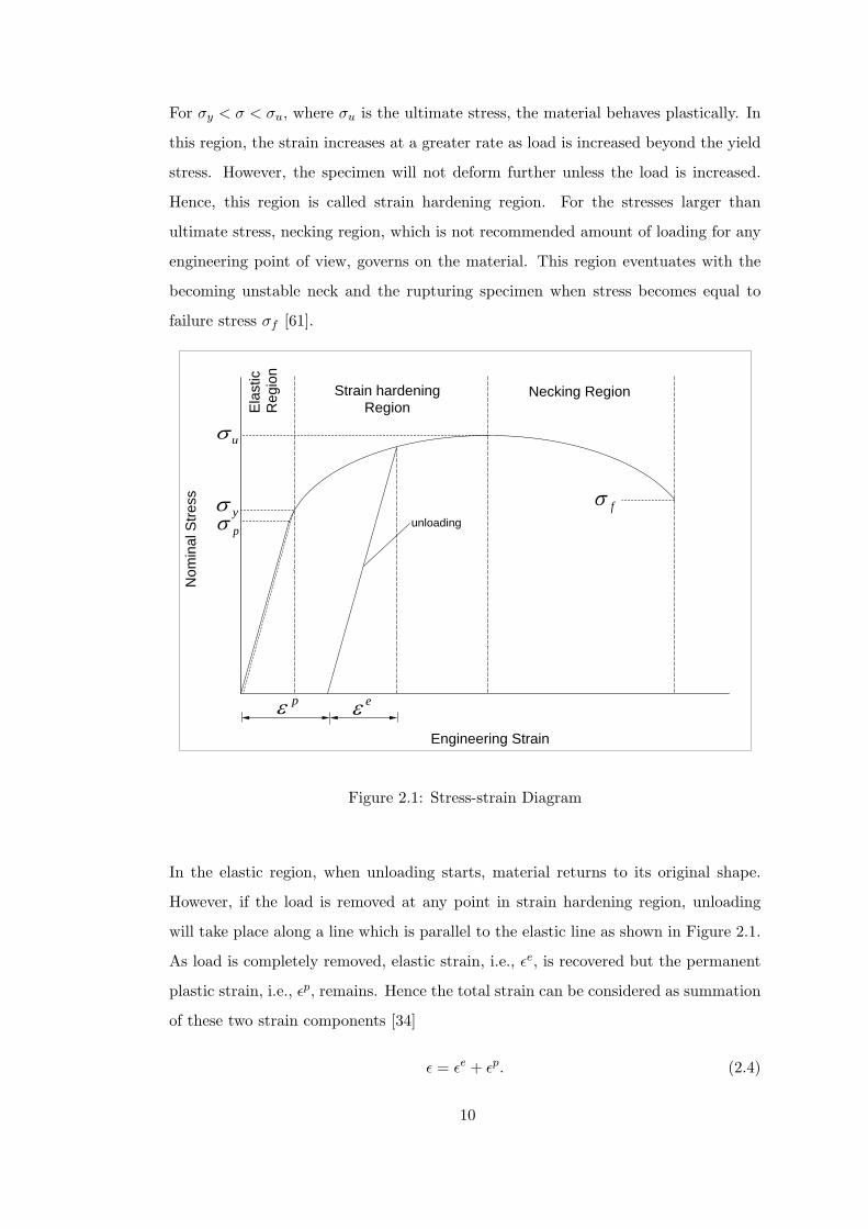
For σy < σ < σu, where σu is the ultimate stress, the material behaves plastically. In

this region, the strain increases at a greater rate as load is increased beyond the yield

stress. However, the specimen will not deform further unless the load is increased.

Hence, this region is called strain hardening region. For the stresses larger than

ultimate stress, necking region, which is not recommended amount of loading for any

engineering point of view, governs on the material. This region eventuates with the

becoming unstable neck and the rupturing specimen when stress becomes equal to

failure stress σf [61].

Engineering Strain

Nom

inal

Stre

ss

Elas

tic

Reg

ion

Strain hardening Region

Necking Region

eεpε

yσ

uσ

fσpσ unloading

Figure 2.1: Stress-strain Diagram

In the elastic region, when unloading starts, material returns to its original shape.

However, if the load is removed at any point in strain hardening region, unloading

will take place along a line which is parallel to the elastic line as shown in Figure 2.1.

As load is completely removed, elastic strain, i.e., εe, is recovered but the permanent

plastic strain, i.e., εp, remains. Hence the total strain can be considered as summation

of these two strain components [34]

ε = εe + εp. (2.4)

10

2.2 Criteria of Yielding

A law defining the limit of elasticity under any possible combination of stresses is called

a criterion of yielding [62]. As seen in Figure 2.1, for the stresses being larger than σy,

behavior of the material is described by using any yielding criterion. Plastic yielding

may depend on the magnitude of the three principal applied stresses, but not on their

directions, since the isotropic case is assumed. Numerous criteria have been proposed

for the yielding of solids, i.e. Maximum stress theory, maximum strain theory, Von

Mises’ criterion, Tresca’s criterion, etc. Among these, Von Mises’ yield criterion and

Tresca’s yield criterion are reasonably simple mathematically and accurate enough to

be highly useful for the initial yield of isotropic materials.

2.2.1 Von Mises’ Yield Criterion

The criterion, which is also known as distortion energy theory, is attributed to Von

Mises [63]. In this theory, failure by yielding occurs at any coordinate of the material

when the distortion energy per unit volume in a state of combined stress becomes equal

to that associated with yielding in a simple tension test [3]. In other words, when the

second deviatoric stress invariant reaches a specified value, yielding emerges. The

principal stress, for σ1 > σ2 > σ3, form of the Von Mises’ yield criterion in simple

tension is

(σ1 − σ2)2 + (σ2 − σ3)

2 + (σ1 − σ3)2 = 2σ2

y , (2.5)

where σy denotes the yield stress. As seen in Eq. (2.5), only the differences of the

principal stresses involved. Therefore, yielding condition is not influenced by any

additional amount to the each stress [3].

Von Mises’ yield criterion finds considerable experimental support in situations in-

volving ductile materials. Consequently, it is in common use in design [3].

2.2.2 Tresca’s Yield Criterion

Tresca’s yield criterion which is also called as maximum shear theory was firstly sug-

gested by Tresca [64]. In this work, he concludes that yielding occurs when the

11

maximum shear stress in the material equals maximum shear stress at yielding in a

simple tension test. In other words, the maximum shear stress is equal to half of dif-

ference between maximum and minimum principal stresses. Hence, for the prescribed

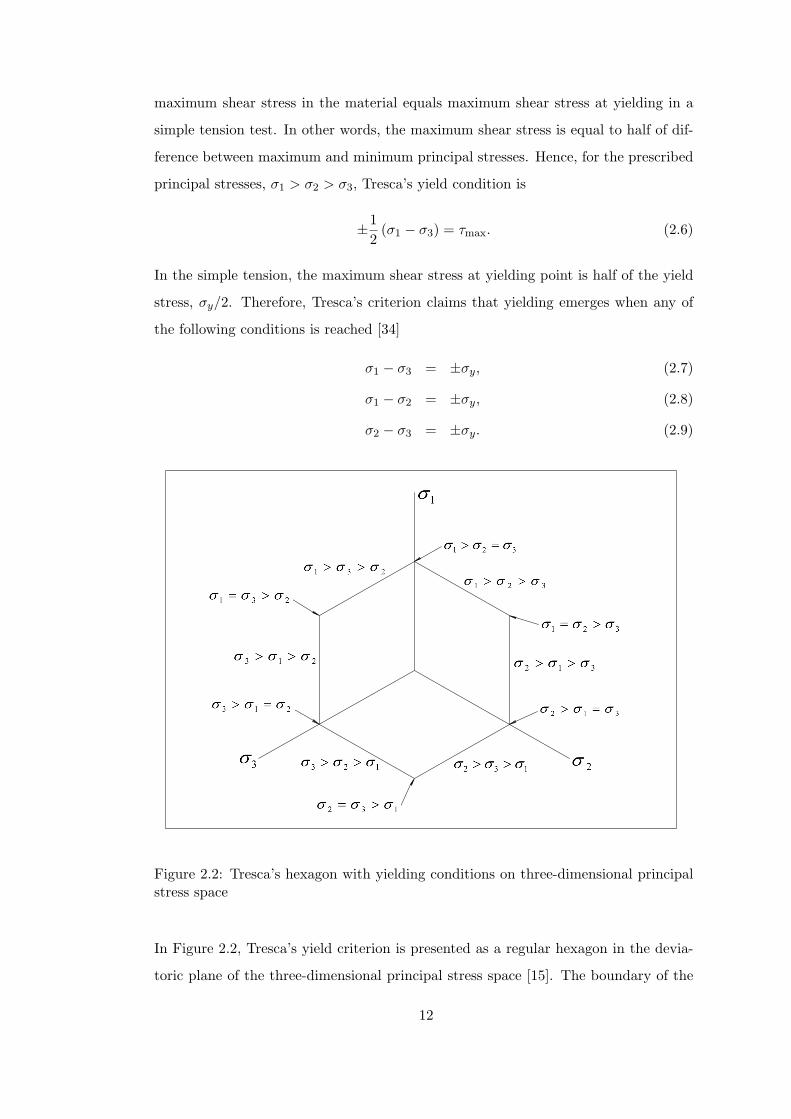
principal stresses, σ1 > σ2 > σ3, Tresca’s yield condition is

±12

(σ1 − σ3) = τmax. (2.6)

In the simple tension, the maximum shear stress at yielding point is half of the yield

stress, σy/2. Therefore, Tresca’s criterion claims that yielding emerges when any of

the following conditions is reached [34]

σ1 − σ3 = ±σy, (2.7)

σ1 − σ2 = ±σy, (2.8)

σ2 − σ3 = ±σy. (2.9)

Figure 2.2: Tresca’s hexagon with yielding conditions on three-dimensional principalstress space

In Figure 2.2, Tresca’s yield criterion is presented as a regular hexagon in the devia-

toric plane of the three-dimensional principal stress space [15]. The boundary of the

12

hexagon marks the onset of yielding and the points outside of the hexagon represents

a yielded state [3]. On this hexagon, each side and edge represent different type of

yielding conditions. At the edge regimes of the Tresca’s hexagon, two of principal

stresses are equal to each other. On the other hand, there exists an inequality be-

tween principal stresses on the side regimes. For example, for the principal stresses

space σ1 > σ3 > σ2 (see the side regime in Figure 2.2), Tresca yielding condition reads

σ1 − σ2 = σy. For the principal stress space σ1 = σ3 > σ2 (edge regime in Tresca’s

hexagon), yielding conditions become σ1−σ2 = σy and σ3−σ2 = σy. Similarly, yield-

ing conditions of remaining side and edge regimes of the Tresca’s hexagon may be

obtained.

Tresca’s yield criterion has a good agreement with experimental results for ductile

materials and the theory offers an additional advantage in its ease of applications [3].

The criterion is mostly chosen for the theoretical treatment of the yielding problem

since it generally makes a closed form solution possible.

2.3 Flow Rule Associated with Yield Criteria

The flow rule is the necessary kinematic assumption for the plastic deformation. It

gives the ratio of the plastic strain increment tensor dεpij and it also defines the direction

of the plastic strain increment vector in the strain space [65]. To obtain the plastic flow

equations, the first approach to plastic strain-stress was suggested by Saint-Venant

[66]. He proposed that the principal axes of the strain increment, but not total strain,

coincides with the axes of the principal stress. A general relationship between the

ratios of the components of strain increment and the stress was firstly suggested by

Levy [67] and then independently by Von Mises [63]. Hence, equations given below

are called Levy-Mises equations.

dεxx

Sxx=

dεyy

Syy=

dεzz

Szz=

dεxy

Sxy=

dεxz

Sxz=

dεyz

Syz= dλ, (2.10)

or more compactly,

dεij = Sijdλ, (2.11)

13

where Sij (i, j : x, y, z) is the stress deviator tensor and dλ is a positive scalar factor

of proportionality and non-zero only when plastic deformation occurs [65]. However,

these equations are only for the rigid materials in which elastic strains are zero because

total strain increments equalized to plastic strain increments. Hence, the extension of

the Levy-Mises equation to allow for the elastic strains was carried out by Prandtl [68].

Then, Reuss [69] suggested the plastic strain increments dεpij related to the deviatoric

stress components by the Prandtl-Reuss equations

dεpxx

Sxx=

dεpyy

Syy=

dεpzz

Szz=

dεpxy

Sxy=

dεpxz

Sxz=

dεpyz

Syz= dλ, (2.12)

or

dεpij = Sijdλ. (2.13)

These equations prove that the principal axes of stress and plastic strain-increment

coincide for isotropic materials [62].

To express a general stress-strain relation, a loading function f(σij) is assumed. Ac-

cording to this assumption, plastic deformation forms only for f(σij) = k and df > 0,

where k depends on the stress state and the strain history. Additionally, the increase

in the plastic strain is a linear function of the increase in stress.

The condition that df = 0 is satisfied by assuming that

dεpij = Gijdf, (2.14)

in which Gij is a symmetric tensor which are supposed to be functions of the stress

components and possibly of the previous strain history [62]. For the case of zero

plastic volume change, assumption of Gij = 0 leads to

Gij = h∂g

∂σij, (2.15)

where g and h are general function of stress and strain flow [62]. Substituting Eq.

(2.15) into Eq. (2.14) gives

dεpij = h

∂g

∂σijdf. (2.16)

14

This equation is firstly obtained by Melan [70]. When the yield function and the

plastic potential function coincide, f = g, following relation is obtained (see Hill [62])

dεpij =

∂f

∂σijdλ. (2.17)

These relations show that plastic flow develops along the normal to the flow surface

∂f/∂σij . Eq. (2.17) is known as associated flow rule with the yield condition since

the plastic flow is associated with the yield criterion. Furthermore, plastic flow can

be expressed in terms of several yield functions as following

dεpij =

∂f1

∂σijdλ1 +

∂f2

∂σijdλ2 + ... +

∂fn

∂σijdλn. (2.18)

2.3.1 Flow Rule Associated with Tresca Yield Function

If the Tresca yield function is taken as the plastic potential, the flow rule associated

with it can be expressed in the light of Section 2.3. By supposing that the ordering in

magnitude of the principal stresses is σ1 > σ2 > σ3 (a side region of Tresca’s hexagon

in principal stress space as seen in Figure 2.2), the corresponding yield function takes

the form

f = F (σij)− 2k = σ1 − σ3 − 2k = 0, (2.19)

where k is the yield value [65]. By substituting the yield function into the associated

flow rule Eq. (2.17), the principal plastic strain increments, dεp1, dεp

2, dεp3, are obtained

as follows:

dεp1 =

∂f

∂σ1dλ = dλ, (2.20)

dεp2 =

∂f

∂σ2dλ = 0, (2.21)

dεp3 =

∂f

∂σ3dλ = −dλ. (2.22)

Similar results can be obtained for the other five possible combinations in algebraic

orders of magnitude of the principal stresses. These are on the side regime of Tresca’s

hexagon in principal space. Furthermore, the increments of plastic strains are parallel

to each other and perpendicular to the side of the hexagon (see Chen and Han [65]).

On the other hand, an example to edge regime of Tresca’s hexagon (see Figure 2.2)

may be σ1 > σ2 = σ3 in principal stress space. In this more involved case, shear slip

may occur along either of two possible maximum shear planes which are [65]

15

i) σmax = σ1, σmin = σ2. Therefore

dεp1 = dλ1, (2.23)

dεp2 = −dλ1, (2.24)

dεp3 = 0, (2.25)

where dλ1 ≥ 0.

ii) σmax = σ1, σmin = σ3. Therefore

dεp1 = dλ2, (2.26)

dεp2 = 0, (2.27)

dεp3 = −dλ2, (2.28)

where for dλ2 ≥ 0. In this case, it is assumed that the resulting plastic strain increment

vector is a linear combination of the two increments (see Eq. (2.18))

dεp1 = dλ1 + dλ2, (2.29)

dεp2 = −dλ1, (2.30)

dεp3 = −dλ2. (2.31)

Similary, for remaining five edges of the Tresca’s hexagon, the associated flow rules

with Tresca’s yield criterion may be obtained.

16

CHAPTER 3

STATEMENT OF THE PROBLEM AND

TEMPERATURE FIELD

3.1 Statement of the Problem

Consider a rotating solid shaft cross section of which is shown in Figure 3.1. The

shaft is subjected to temperature cycle. In formulation, cylindrical polar coordinates,

i.e. r is radial, θ is circumferential, and z is axial directions, are considered. Notation

of Timoshenko and Goodier [1] is followed. Hence, σi and εi denote a normal stress

and a normal strain component (i : r, θ, z), respectively, u is the radial component

of the displacement vector, ρ is the mass density of the shaft material, and ω is

constant angular speed of rotation. The subject of the investigation is a rotating

elastic-perfectly plastic solid shaft with outer radius b with stress free cylindrical

surface (see Figure 3.1) [12]

r = b : σr = 0. (3.1)

Another mechanical boundary condition is that axial force Fz on any cross-section

vanishes since the ends of the shaft are free [12]

Fz = 2π

∫ b

0σzrdr = 0. (3.2)

For completeness, it is stated that the radial displacement component has to comply

with the condition (see [12])

u (0) = 0, (3.3)

since shaft is solid. A state of generalized plane strain, i. e.

εz = ε0 = Constant, (3.4)

17

where the axial strain ε0 depends on the angular speed and the temperature field, is

considered. Additionally, infinitesimal deformations are presumed. Since end effects

are ignored and cylindrical symmetry is presumed, the principal directions of stress and

strain are the radial, circumferential and axial directions [11]. As already mentioned,

the material is assumed to obey Tresca‘s yield criterion and the associated flow rule

with it [32], [65]. For a linear temperature dependence the yield stress, σth, reads

σth = σ0 (1− βT ) , (3.5)

where σ0 denotes the uniaxial yield limit at reference temperature and β the temper-

ature dependence parameter of the material [45], [56]. T , which will be examined in

the Section 3.2, means the difference of absolute and reference temperatures.

Figure 3.1: Sketch of the rotating solid shaft subjected to temperature cycle

3.2 Temperature Field

Temperature cycle that is applied to outer surface of the shaft is sketched in Figure

3.2. As seen in the figure, the temperature at the surface of the shaft is increased

18

linearly and slowly up to maximum temperature value Tm in time tt. Then, it is held

constant throughout t = tc. Finally, it is decreased linearly at the same rate to the

reference temperature until t = 2tt + tc. For t > 2tt + tc, surface temperature remains

at the reference temperature value.

0.0

0.2

0.4

0.6

0.8

1.0

1.2

0.0 0.4 0.8 1.2 1.6 2.0 2.4 2.8 3.2 3.6 4.0

Time

Tem

pera

ture

mT

tt ct tt + ct tt +2

),( tbT

Figure 3.2: Prescribed surface temperature of the shaft

To model this temperature cycle, the surface temperature of the shaft is prescribed

as a sectionally linear function of time [56]. Thus, the heat conduction problem is

described by the following differential equation:

κ

r

∂

∂r

[r∂T (r, t)

∂r

]=

∂T (r, t)∂t

, (3.6)

in which κ denotes the thermal diffusivity, subject to the initial condition

T (r, 0) = 0 for 0 ≤ r ≤ b, (3.7)

19

and to the boundary condition (see Figure 3.2)

T (b, t) =

(Tm/tt) t for 0 < t ≤ tt

Tm for tt < t ≤ tt + tc

Tm − (Tm/tt) (t− tt − tc) for tt + tc < t ≤ 2tt + tc

0 for t > 2tt + tc

. (3.8)

0.0

1.0

2.0

3.0

0.0 0.4 0.8 1.2 1.6 2.0 2.4 2.8 3.2 3.6 4.0 4.4 4.8

-3.0

-2.0

-1.0

0.0

1.0

2.0

3.0

0.0 0.4 0.8 1.2 1.6 2.0 2.4 2.8 3.2 3.6 4.0 4.4 4.8

bT

bT

mT

tt ct tt + ct tt +2 t

t

( )ttT tm /

( )( )ttm tttT −− /

( )( )cttm ttttT −−− /

( )( )cttm ttttT −− 2/

Figure 3.3: Description of surface temperature with linear function

Solution of the heat conduction equation has been obtained in [71] for zero initial

temperature (Eq. (3.7)) and the surface temperature of T (b, t) = (Tm/tt) t as following

T (r, t) =Tm

tt

[(t− b2 − r2

4κ

)+

2κb

∞∑n=1

e−κγ2nt J0 (rγn)

γ3nJ1 (bγn)

], (3.9)

where J0 and J1 indicate Bessel functions of the first kind of order zero and one,

20

respectively, and the γn are the positive roots of

J0 (bγ) = 0. (3.10)

This solution is valid for time interval 0 < t ≤ tt since boundary condition in this

interval is T (b, t) = (Tm/tt) t. In order to find the solution for the range of t > tt,

different linear functions are defined as shown in the Figure 3.3. By superposition of

these linear functions, the boundary condition for each time interval in Eq. (3.8) can

be obtained.

Hence, the solution of heat conduction problem (3.9) can be adapted for all time

intervals as

T (r, t) =

T (r, t) for 0 < t ≤ tt

T (r, t)− T (r, t− tt) for tt < t ≤ tt + tc

T (r, t)− T (r, t− tt)− T (r, t− tt − tc) for tt + tc < t ≤ 2tt + tc

T (r, t)− T (r, t− tt)− T (r, t− tt − tc)

+T (r, t− 2tt − tc) for t > 2tt + tc

.

(3.11)

21

CHAPTER 4

BASIC EQUATIONS AND ANALYTICAL

SOLUTIONS OF ELASTIC AND PLASTIC REGIONS

4.1 Basic Equations

Equation of motion that is derived by using Newton’s second law, is the primary

equation that is used for the mathematical derivation of elastic and plastic regions.

General form of equation of motion in radial direction is as derived in [1]

∂σr

∂r+

1r

∂τrθ

∂θ+

σr − σθ

r+ R = 0, (4.1)

where τrθ is shear stress and R is component of body force. In this problem, the shear

stress τrθ vanishes because of the symmetry [1]. Hence, terms of ∂τrθ/∂θ drops in Eq.

(4.1). Additionally, the body force R is described with neglecting weight of the shaft

as

R = ρω2r + ρ∂2u

∂t2, (4.2)

where ρ is mass per unit volume of the material and ω is constant angular rotation

speed of the shaft [1], [4]. In this equation, the first term, ρω2r, is an inertia force that

occurs because of rotation [1]. The second term, i.e. ρ(∂2u/∂t2

), is another inertia

term that is formed due to thermally induced wave phenomena. In case of sudden

temperature change in a material, such as quenching of a hot shaft, this term has a

significant effect on the body force. On the other hand, if the temperature is altered

slowly in time, this inertia force does not influence the material [4]. Hence, the second

term in the body force drops in this study, ρ∂2u∂t2

= 0, since the temperature cycle

(in Figure 3.2) is applied to the surface of the shaft slowly. Therefore, for constant

angular speed, in the absence of thermally induced wave phenomena, neglecting weight

22

of the shaft and in case of cylindrical symmetry, the equation of motion for the radial

direction in Eq. (4.1) takes the form

(rσr)′ − σθ = −ρω2r2. (4.3)

In this equation, a prime denotes differentiation with respect to r as radial and cir-

cumferential stresses are independent of circumferential direction θ.

Since the treatment is restricted to small deformations, radial and circumferential

strain components are described with the following geometric relations in case of

cylindrical symmetry as

εr = u′, εθ =u

r. (4.4)

Another basic relation is Generalized Hooke’s law [4], which follows as

εr =1

2 (1 + ν) G[σr − ν (σθ + σz)] + εp

r + αT, (4.5a)

εθ =1

2 (1 + ν) G[σθ − ν (σr + σz)] + εp

θ + αT, (4.5b)

εz = ε0 =1

2 (1 + ν) G[σz − ν (σr + σθ)] + εp

z + αT, (4.5c)

where ν denotes Poison’s ratio, G is modulus of rigidity, εpi are plastic strain compo-

nents and α is the coefficient of thermal expansion in material [56], [59]. It is presumed

that the strains are additively composed of elastic, plastic and thermal parts in these

equations.

4.2 Elastic Region

In the elastic deformation, Eqs. (4.5a−4.5c) are recovered by setting εpi = 0. Axial

stress is determined in terms of radial and circumferential stresses from Hooke’s law

(4.5c) in a state of generalized plane strain (Eq. (3.4)) as

σz = ν (σr + σθ) + 2G (1 + ν) [ε0 − αT (r, t)] . (4.6)

On the one hand, by making use of geometric relations (4.4) and Hooke’s law in

radial and circumferential directions (4.5a) and (4.5b), following stress components

are derived in terms of radial displacement and its derivative with help of Eq. (4.6)

23

σr =2G

r(1− 2ν)[νu + r(1− ν)u′ + rνε0 − rα(1 + ν)T (r, t)

], (4.7)

σθ =2G

r(1− 2ν)[(1− ν) u + rνu′ + rνε0 − rα(1 + ν)T (r, t)

]. (4.8)

Inserting the stresses in Eqs. (4.7) and (4.8) into the equation of motion (4.3), one

obtains the nonhomogenous Euler equation for radial displacement

r2 d2u

dr2+ r

du

dr− u = − r2

(1− ν)

[1− 2ν

2Gρω2r − α(1 + ν)T ′ (r, t)

]. (4.9)

Solution of homogeneous part of this equation is obtained effortlessly as

uh =C1

r+ C2r, (4.10)

in which C1 and C2 are arbitrary integration constants. The particular solution of the

problem is integrated by the method of variation of parameters since the equation is

suitable to the form of

d2u

dr2+

1r

du

dr− u

r2= F (r). (4.11)

as given in [72]. In this method, particular solution of the equation is obtained by

using

up(r) = Y1(r)u1(r) + Y2(r)u2(r), (4.12)

where Y1(r) and Y2(r) are defined by using homogeneous solution of the problem

(4.10) as

Y1(r) =1r, (4.13)

Y2(r) = r, (4.14)

and

u1(r) = −∫

Y2(r)F (r)W (r)

dr, (4.15a)

u2(r) =∫

Y1(r)F (r)W (r)

dr, (4.15b)

in which Wronskian of the system is obtained by using

W (r) = Y1(r)dY2(r)

dr− dY1(r)

drY2(r), (4.16)

24

as

W (r) =2r. (4.17)

and F (r) is the non-homogeneous part of the equation as

F (r) = − 1(1− ν)

[1− 2ν

2Gρω2r − α(1 + ν)T ′ (r, t)

]. (4.18)

Hence, particular solution is integrated as

up = −(1− 2ν)ρω2r3

16G(1− ν)+

α(1 + ν)r(1− ν)

∫ r

0T (ξ, t) ξdξ. (4.19)

The integral involved in this equation can be evaluated analytically. The result is∫ r

0T (ξ, t) ξdξ =

Tm

tt

[(t− b2

4κ+

r2

8κ

)r2

2+

2κb

∞∑n=1

e−κγ2nt rJ1 (rγn)

γ4nJ1 (bγn)

]. (4.20)

For the general solution of the Eq. (4.9),

u = uh + up (4.21)

is used. The result is

u =C1

r+ C2r −

(1− 2ν)ρω2r3

16G(1− ν)+

α(1 + ν)r(1− ν)

∫ r

0T (ξ, t) ξdξ. (4.22)

From Eqs. (4.7) and (4.8), radial and circumferential stress components are derived

as

σr = −2GC1

r2+

2G

1− 2ν(C2 + νε0)−

18(1− ν)

[(3− 2ν)ρω2r2

+16Gα(1 + ν)

r2

∫ r

0T (ξ, t) ξdξ

], (4.23)

σθ =2GC1

r2+

2G

1− 2ν(C2 + νε0)−

18(1− ν)

(1 + 2ν)ρω2r2

+16Gα(1 + ν)

r2

[r2T (r, t)−

∫ r

0T (ξ, t) ξdξ

]. (4.24)

Then, substituting these stresses into Eq. (4.6) gives

σz =2G

1− 2ν[2νC2 + (1− ν)ε0]−

12(1− ν)

[νρω2r2 + 4Gα(1 + ν)T (r, t)

]. (4.25)

25

The solution presented here is in agreement with those in [12],[44],[45]. On the other

hand, it should be mentioned that as r → 0 (at the center of the shaft) the terms

containing the temperature T (r, t) are finite in all equations in consistence with the

physics of the problem. In this context, following integrals that are located in the

equations are calculated in the limiting case by L’Hopital’s Rule to prevent computa-

tional singularity [4]

limr→0

[1r

∫ r

0T (ξ, t) ξdξ

]= lim

r→0rT (r, t) = 0, (4.26)

limr→0

[1r2

∫ r

0T (ξ, t) ξdξ

]= lim

r→0

rT (r, t)2r

=T (0, t)

2. (4.27)

Finally, axial force is determined by assuming the elastic region is bounded in δ ≤ r ≤

λ with help of Eq. (4.25)

F ez = 2π

∫ λ

δσzrdr = 2π

G

(λ2 − δ2

)1− 2ν

[2νC2 + (1− ν)ε0]

− 18(1− ν)

[(λ4 − δ4

)νρω2 + 16Gα(1 + ν)

∫ λ

δT (ξ, t) ξdξ

], (4.28)

to make use of condition (3.2) for further calculations.

4.3 Plastic (Edge Regime) Region I

In the plastic region I, the stress state is in an edge regime of Tresca’s hexagon in

the principal stress space with the inequality of σr = σθ > σz. Hence, Tresca’s yield

condition leads to

σθ − σz = σth, σr − σz = σth, (4.29)

where σth is the yield stress and as defined in Eq. (3.5). Accordingly, for this plastic

region, Tresca’s yielding functions are described as

f1 = σθ − σz − σth = 0, (4.30)

f2 = σr − σz − σth = 0. (4.31)

The flow rule associated with the yielding condition reads

dεpi =

2∑j=1

∂fj

∂σidλj , (4.32)

26

where the subscript i denotes a principal direction and dλj is a positive scalar factor

of proportionality [65]. Hence, for this plastic region, plastic strain increments are

dεpr =

∂f1

∂σrdλ1 +

∂f2

∂σrdλ2 = dλ2, (4.33)

dεpθ =

∂f1

∂σθdλ1 +

∂f2

∂σθdλ2 = dλ1, (4.34)

dεpz =

∂f1

∂σzdλ1 +

∂f2

∂σzdλ2 = −dλ1 − dλ2. (4.35)

Furthermore in case of a monotonically increasing load parameters, the radial and

circumferential plastic strains are positive (εpr > 0 and εp

θ > 0), and axial plastic strain

is the negative sum of the other two directions due to the plastic incompressibility

εpz = −

(εpr + εp

θ

). (4.36)

According to the yield condition (4.29), circumferential and axial stresses can be

expressed in term of radial stress as

σθ = σr, (4.37)

σz = σr − σth. (4.38)

Inserting Eq. (4.37) into the equation of motion (4.3) gives

rσ′r + ρω2r2 = 0. (4.39)

Integration of this equation leads to

σr = C3 −12ρω2r2, (4.40)

where C3 is an integration constant. It should be also kept in mind that σθ = σr. In

order to find out axial stress component, Eqs. (3.5) and (4.38) are combined:

σz = C3 −12ρω2r2 − σ0 [1− βT (r, t)] . (4.41)

By taking into account plane strain assumption (3.4) and geometric relations (4.4),

summation of strains can be displayed as (see [73])

εr + εθ + εz = u′ +u

r+ ε0. (4.42)

Here, each strain can be written in terms of stresses and plastic strains by using

Hooke’s law (4.5). Furthermore, summation of the plastic strains equals zero because

27

of plastic incompressibility (4.36). Hence, only stress terms remain in the equation.

This equation and additionally Eqs. (4.37), (4.40) and (4.41) are used to derive first

order linear differential equation for radial displacement:

u′ +u

r=

14G (1 + ν)

(1− 2ν)

(6C3 − 2σ0 − 3ρω2r2

)+2 [6Gα (1 + ν) + β (1− 2ν) σ0]T (r, t) − ε0. (4.43)

This equation is in the form of linear Bernoulli equation [72] as

u′ + p(r)u = q(r), (4.44)

with the solution of

u =1

a(r)

∫a(r)q(r)dr +

C

a(r), (4.45)

where C is a constant and a(r) is defined as

a(r) = e∫

p(r)dr. (4.46)

In Eq. (4.43)

p(r) =1r, (4.47)

a(r) = r, (4.48)

q(r) =1

4G (1 + ν)(1− 2ν)

(6C3 − 2σ0 − 3ρω2r2

)+2 [6Gα (1 + ν) + β (1− 2ν) σ0]T (r, t) − ε0. (4.49)

The general solution is adapted as

u =C4

r− ε0r

2+

14Gr (1 + ν)

(1− 2ν) r2

4(12C3 − 4σ0 − 3ρω2r2

)+2 [6Gα (1 + ν) + β (1− 2ν) σ0]

∫ r

0T (ξ, t) ξdξ

, (4.50)

in which C4 is fourth integration constant of the problem. The integral here has been

evaluated before and given in Eq. (4.20). The plastic parts of the strains are found as

the differences of the total strains and their elastic and thermal parts together with

Eqs. (4.4), (4.37), (4.40), (4.41) and (4.50) as

εpr = −C4

r2− ε0

2+

116G (1 + ν)

(1− 2ν)

(4C3 − 5ρω2r2

)− 4σ0

−8 [6Gα (1 + ν) + β (1− 2ν) σ0]r2

∫ r

0T (ξ, t) ξdξ

+8 [4Gα (1 + ν) + β (1− ν) σ0]T (r, t) , (4.51)

28

εpθ =

C4

r2− ε0

2+

116G (1 + ν)

(1− 2ν)

(4C3 + ρω2r2

)− 4σ0

+8 [6Gα (1 + ν) + β (1− 2ν) σ0]

r2

∫ r

0T (ξ, t) ξdξ

−8 [2Gα (1 + ν)− βνσ0]T (r, t) , (4.52)

εpz =

(1− 2ν)(ρω2r2 − 2C3

)+ 2σ0

4G (1 + ν)+ ε0 −

[α +

βσ0

2G (1 + ν)

]T (r, t) . (4.53)

The axial force integral for the plastic region I is calculated with the help of Eq. (4.41)

as

FPIz = 2π

∫ λ

δσzrdr = 2π

(λ2 − δ2

)2

[C3 − σ0 −

(λ2 + δ2

)ρω2

4

]

+βσ0

∫ λ

δT (ξ, t) ξdξ.

. (4.54)

Here, it should be noted that all expressions that are derived in this region for T (r, t) =

0, recovers the equations given in [12].

4.4 Plastic (Side Regime) Region II

Governing equation for this region is obtained by a procedure similar to the one

outlined in [21] as following. In plastic region II, the principal stresses satisfy σθ >

σr > σz. The stress image points are on a side regime of Tresca’s hexagon in principal

stress space. At this point, the yield condition takes the form

σθ − σz = σth. (4.55)

Accordingly, for this plastic region Tresca’s yielding function is described by

f1 = σθ − σz − σth = 0. (4.56)

By making use of Eq. (4.32) plastic strain increments become

dεpr =

∂f1

∂σrdλ1 = 0, (4.57)

dεpθ =

∂f1

∂σθdλ1 = dλ1, (4.58)

dεpz =

∂f1

∂σzdλ1 = −dλ1. (4.59)

and plastic strains satisfy εpr = 0, εp

θ > 0, and εpz < 0. In the absence of plastic

29

predeformation, the associated flow rule becomes

εpr = 0, (4.60)

εpθ = −εp

z. (4.61)

Hence, the radial strain consists of an elastic and thermal parts only:

εr =1

2 (1 + ν) G[σr − ν (σθ + σz)] + αT. (4.62)

Here and further, axial stress is eliminated by using

σz = σθ − σth, (4.63)

that is obtained from yield condition (4.55). Thus, axial plastic strain component may

be expressed by using Eqs. (4.5c) and (3.5) as

εpz = ε0 +

νσr − (1− ν) σθ + σ0 (1− βT )2G (1 + ν)

− αT. (4.64)

By using Eq. (4.64) circumferential strain leads to

εθ = −ε0 −1

G (1 + ν)

νσr − (1− ν)

[σθ −

σ0

2(1− βT )

]+ 2αT. (4.65)

Then Eqs. (4.62) and (4.65) are substituted into geometric relations (4.4) to get

σr =2G

(1− 2ν) r

[ν (u + ε0r) + (1− ν) u′r − α (1 + ν) rT (r, t)

], (4.66)

σθ =1

2 (1− 2ν)

2G

(u

r+ 2νu′ + ε0

)+ (1− 2ν) σ0

− [4Gα (1 + ν) + β (1− 2ν) σ0]T (r, t) . (4.67)

Inserting these equations into Eq. (4.3) field equation for plastic region II is obtained:

r2u′′ + ru′ − u

2 (1− ν)=

r

4G (1− ν)[(1− 2ν)

(2Gε0 + σ0 − 2ρω2r2

)−β (1− 2ν) σ0T (r, t) + 4Gα (1 + ν)

×rT ′ (r, t)]. (4.68)

Solution of homogeneous part of field equation is

uh = C5rM +

C6

rM, (4.69)

30

where C5 and C6 are arbitrary integration constants and

M =

√1

2 (1− ν). (4.70)

For the particular solution, method of Variation of parameter is used as defined in the

elastic region. For Y1(r) = rM , and Y2(r) = 1/rM , Wronksian is calculated by using

Eq. (4.16) as

W (r) =−2M

r. (4.71)

In Eq. (4.68), it is visible that

F (r) =1r2

r

4G (1− ν)[(1− 2ν)

(2Gε0 + σ0 − 2ρω2r2

)−β (1− 2ν) σ0T (r, t) + 4Gα (1 + ν) rT ′ (r, t)

] . (4.72)

By using Eqs. (4.12) and (4.15) particular solution is compiled as

up = ε0r −(1− 2ν) ρω2r3

G (17− 18ν)+

σ0

2G

r − β (1− 2ν)

4M (1− ν)

[rM

∫ r

0T (ξ, t) ξ−Mdξ

−r−M

∫ r

0T (ξ, t) ξMdξ

]+

α (1 + ν)2M (1− ν)

[rM

∫ r

0

∂T (ξ, t)∂ξ

ξ1−Mdξ

−r−M

∫ r

0

∂T (ξ, t)∂ξ

ξ1+Mdξ

]. (4.73)

Integration by parts is applied to get rid of derivatives of temperature in the integrals

and following solutions are obtained∫ r

0

∂T (ξ, t)∂ξ

ξ1−Mdξ = r1−MT (r, t)− (1−M)∫ r

0T (ξ, t) ξ−Mdξ, (4.74)∫ r

0

∂T (ξ, t)∂ξ

ξ1+Mdξ = r1+MT (r, t)− (1 + M)∫ r

0T (ξ, t) ξMdξ. (4.75)

The integrals in Eqs. (4.74) and (4.75) are amenable to analytical treatment. The

results are∫ r

0T (ξ, t) ξMdξ =

Tm

tt

r1+M [(1 + M)r2 − (3 + M)(b2 − 4κt)]

4κ(1 + M)(3 + M)

+2

κb(1 + M)

∞∑n=1

e−κγ2nt r

1+MFH(a1, a2, a3; z)γ3

nJ1 (bγn)

, (4.76)

where FH(a1, a2, a3; z) is a hypergeometric function and is described as

FH(a1, a2, a3; z) = 1 +a1

a2a3z +

a1(1 + a1)2a2(1 + a2)a3(1 + a3)

z2

+a1(1 + a1)(2 + a1)

6a2(1 + a2)(2 + a2)a3(1 + a3)(2 + a3)z3 + · · · (4.77)

31

and where

a1 =12

+M

2, (4.78)

a2 = 1, (4.79)

a3 =32

+M

2, (4.80)

z = −14r2γ2

n. (4.81)

and ∫ r

0T (ξ, t) ξ−Mdξ =

Tm

tt

r1−M [(1−M)r2 − (3−M)(b2 − 4κt)]

4κ(1−M)(3−M)

+2

κb(1−M)

∞∑n=1

e−κγ2nt r

1−MFH(a1, a2, a3; z)γ3

nJ1 (bγn)

, (4.82)

where FH(a1, a2, a3; z) is same as in Eq. (4.77) and

a1 =12− M

2, (4.83)

a2 = 1, (4.84)

a3 =32− M

2, (4.85)

z = −14r2γ2

n. (4.86)

After some simplification and with Eq. (4.21), radial displacement is acquired as

u = C5rM +

C6

rM+ r

(ε0 +

σ0

2G

)− (1− 2ν) ρω2r3

G (17− 18ν)

+1

8GM (1− ν)

4Gα (1 + M) (1 + ν) + β (1− 2ν) σ0

rM

∫ r

0T (ξ, t) ξMdξ

−rM [4Gα (1−M) (1 + ν) + β (1− 2ν) σ0]∫ r

0T (ξ, t) ξ−Mdξ

. (4.87)

Substituting radial displacement and its radial derivative into Eqs. (4.66) and (4.67)

gives radial and circumferential stresses

σr =2G

(1− 2ν) r

C5 [M (1− ν) + ν] rM − C6 [M (1− ν)− ν] r−M + (1 + ν) ε0r

+σ0r

2G

− 2 (3− 2ν) ρω2r2

17− 18ν− 1

4M (1− ν) (1− 2ν) r

[M (1− ν) + ν]

× [4Gα (1−M) (1 + ν) + β (1− 2ν) σ0] rM

∫ r

0T (ξ, t) ξ−Mdξ

+[M (1− ν)− ν] [4Gα (1 + M) (1 + ν) + β (1− 2ν) σ0]

rM

×∫ r

0T (ξ, t) ξMdξ

, (4.88)

32

σθ =G

(1− 2ν) r

[C5 (1 + 2Mν) rM + C6 (1− 2Mν) r−M + 2 (1 + ν) ε0r

+σ0r

G

]− (1 + 6ν) ρω2r2

17− 18ν− 1

8M (1− ν) (1− 2ν) r

(1 + 2Mν)

× [4Gα (1−M) (1 + ν) + β (1− 2ν) σ0] rM

∫ r

0T (ξ, t) ξ−Mdξ

−(1− 2Mν) [4Gα (1 + M) (1 + ν) + β (1− 2ν) σ0]rM

∫ r

0T (ξ, t) ξMdξ

−4Gα (1 + ν) + β (1− ν) σ0

2 (1− ν)T (r, t) . (4.89)

Axial stress component is obtained by making use of Eq. (4.63) as

σz =G

(1− 2ν) r

[C5 (1 + 2Mν) rM + C6 (1− 2Mν) r−M + 2 (1 + ν) ε0r

+2νσ0r

G

]− (1 + 6ν) ρω2r2

17− 18ν− 1

8M (1− ν) (1− 2ν) r

(1 + 2Mν)

× [4Gα (1−M) (1 + ν) + β (1− 2ν) σ0] rM

∫ r

0T (ξ, t) ξ−Mdξ

−(1− 2Mν) [4Gα (1 + M) (1 + ν) + β (1− 2ν) σ0]rM

∫ r

0T (ξ, t) ξMdξ

−4Gα (1 + ν)− β (1− ν) σ0

2 (1− ν)T (r, t) . (4.90)

Finally, axial and circumferential plastic strains are derived with the help of Eqs.

(4.61) and (4.64) as

εpz = −εp

θ = − 12r

(C5r

M +C6

rM

)+

(1− 2ν) ρω2r2

2G (17− 18ν)

+1

16GM (1− ν) r

[4Gα (1−M) (1 + ν) + β (1− 2ν) σ0] rM

×∫ r

0T (ξ, t) ξ−Mdξ − [4Gα (1 + M) (1 + ν) + β (1− 2ν) σ0]

rM

×∫ r

0T (ξ, t) ξMdξ

− βσ0

4GT (r, t) . (4.91)

Axial force integral is more complicated than those of previous regions because of

the necessity for evaluation of double integrals that are obtained by using Eq. (3.2).

33

Method of integration by parts helps to transform double integrals into single ones as∫ λ

δr−M

(∫ r

0T (ξ, t) ξMdξ

)dr =

λ1−M

1−M

∫ λ

0T (ξ, t) ξMdξ

− δ1−M

1−M

∫ δ

0T (ξ, t) ξMdξ

− 11−M

∫ λ

δT (ξ, t) ξdξ, (4.92)∫ λ

δrM

(∫ r

0T (ξ, t) ξ−Mdξ

)dr =

λ1+M

1 + M

∫ λ

0T (ξ, t) ξ−Mdξ

− δ1+M

1 + M

∫ δ

0T (ξ, t) ξ−Mdξ

− 11 + M

∫ λ

δT (ξ, t) ξdξ. (4.93)

With the help of these integrations and after some simplifications, axial force integral

for plastic region II is calculated as

FPIIz = 2π

1

1− 2ν

(λ1+M − δ1+M

)(1 + 2Mν) GC5

1 + M

+

(λ1−M − δ1−M

)(1− 2Mν) GC6

1−M+

(λ2 − δ2

)[(1 + ν) Gε0 + νσ0]

−(λ4 − δ4

)(1 + 6ν) ρω2

4 (17− 18ν)− S1

1 + M

[λ1+M

∫ λ

0T (ξ, t) ξ−Mdξ

−δ1+M

∫ δ

0T (ξ, t) ξ−Mdξ

]+

S2

1−M

[λ1−M

∫ λ

0T (ξ, t) ξMdξ

−δ1−M

∫ δ

0T (ξ, t) ξMdξ

]+

(S1

1 + M− S2

1−M− S3

)×

∫ λ

δT (ξ, t) ξdξ

, (4.94)

in which

S1 =(1 + 2Mν) [4 (1−M) (1 + ν) Gα + (1− 2ν) σ0β]

8M (1− ν) (1− 2ν), (4.95)

S2 =(1− 2Mν) [4 (1 + M) (1 + ν) Gα + (1− 2ν) σ0β]

8M (1− ν) (1− 2ν), (4.96)

S3 =4 (1 + ν) Gα− (1− ν) σ0β

2 (1− ν). (4.97)

4.5 Predeformed Elastic Region

Predeformed elastic region is an elastic region that includes permanent plastic de-

formations, which have been occured in elastic-plastic state. It becomes valid after

34

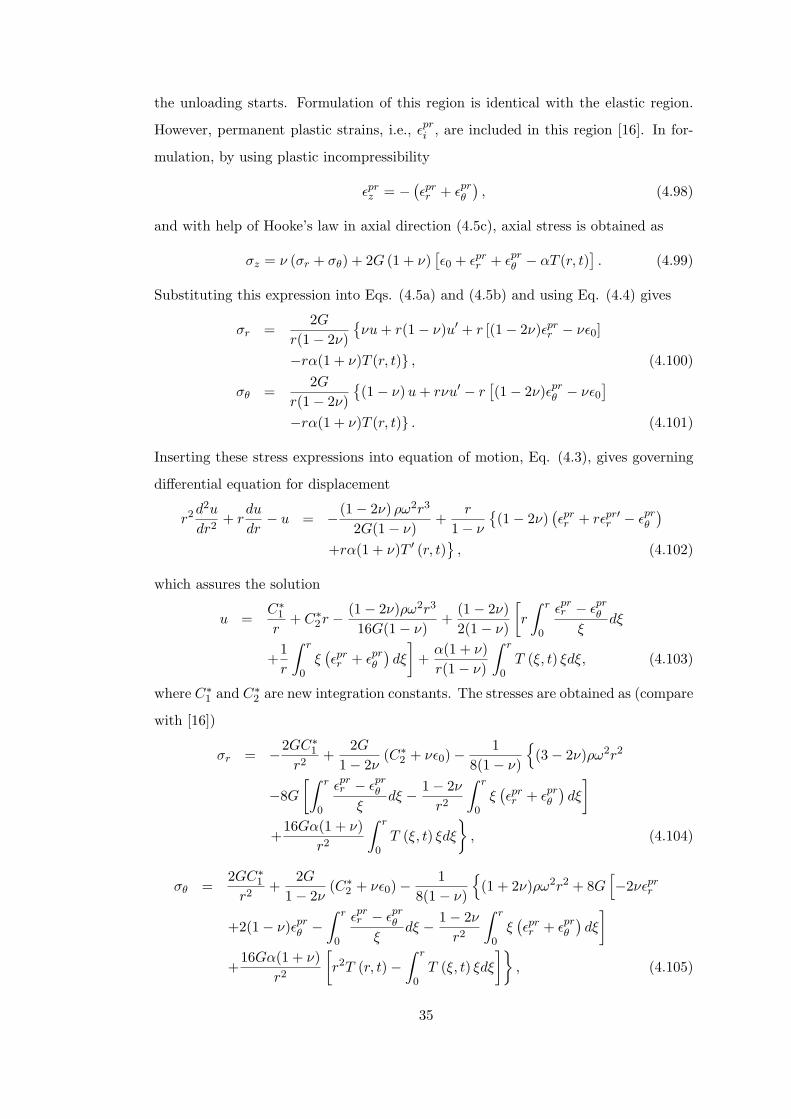
the unloading starts. Formulation of this region is identical with the elastic region.

However, permanent plastic strains, i.e., εpri , are included in this region [16]. In for-

mulation, by using plastic incompressibility

εprz = −

(εprr + εpr

θ

), (4.98)

and with help of Hooke’s law in axial direction (4.5c), axial stress is obtained as

σz = ν (σr + σθ) + 2G (1 + ν)[ε0 + εpr

r + εprθ − αT (r, t)

]. (4.99)

Substituting this expression into Eqs. (4.5a) and (4.5b) and using Eq. (4.4) gives

σr =2G

r(1− 2ν)νu + r(1− ν)u′ + r [(1− 2ν)εpr

r − νε0]

−rα(1 + ν)T (r, t) , (4.100)

σθ =2G

r(1− 2ν)(1− ν) u + rνu′ − r

[(1− 2ν)εpr

θ − νε0]

−rα(1 + ν)T (r, t) . (4.101)

Inserting these stress expressions into equation of motion, Eq. (4.3), gives governing

differential equation for displacement

r2 d2u

dr2+ r

du

dr− u = −(1− 2ν) ρω2r3

2G(1− ν)+

r

1− ν

(1− 2ν)

(εprr + rεpr′

r − εprθ

)+rα(1 + ν)T ′ (r, t)

, (4.102)

which assures the solution

u =C∗

1

r+ C∗

2r − (1− 2ν)ρω2r3

16G(1− ν)+

(1− 2ν)2(1− ν)

[r

∫ r

0

εprr − εpr

θ

ξdξ

+1r

∫ r

0ξ(εprr + εpr

θ

)dξ

]+

α(1 + ν)r(1− ν)

∫ r

0T (ξ, t) ξdξ, (4.103)

where C∗1 and C∗

2 are new integration constants. The stresses are obtained as (compare

with [16])

σr = −2GC∗1

r2+

2G

1− 2ν(C∗

2 + νε0)−1

8(1− ν)

(3− 2ν)ρω2r2

−8G

[∫ r

0

εprr − εpr

θ

ξdξ − 1− 2ν

r2

∫ r

0ξ(εprr + εpr

θ

)dξ

]+

16Gα(1 + ν)r2

∫ r

0T (ξ, t) ξdξ

, (4.104)

σθ =2GC∗

1

r2+

2G

1− 2ν(C∗

2 + νε0)−1

8(1− ν)

(1 + 2ν)ρω2r2 + 8G

[−2νεpr

r

+2(1− ν)εprθ −

∫ r

0

εprr − εpr

θ

ξdξ − 1− 2ν

r2

∫ r

0ξ(εprr + εpr

θ

)dξ

]+

16Gα(1 + ν)r2

[r2T (r, t)−

∫ r

0T (ξ, t) ξdξ

], (4.105)

35

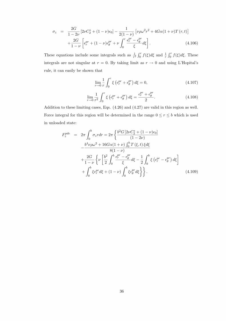
σz =2G

1− 2ν[2νC∗

2 + (1− ν)ε0]−1

2(1− ν)[νρω2r2 + 4Gα(1 + ν)T (r, t)

]+

2G

1− ν

[εprr + (1− ν)εpr

θ + ν

∫ r

0

εprr − εpr

θ

ξdξ

]. (4.106)

These equations include some integrals such as 1r2

∫ r0 f(ξ)dξ and 1

r

∫ r0 f(ξ)dξ. These

integrals are not singular at r = 0. By taking limit as r → 0 and using L’Hopital’s

rule, it can easily be shown that

limr→0

1r

∫ r

0ξ(εprr + εpr

θ

)dξ = 0, (4.107)

limr→0

1r2

∫ r

0ξ(εprr + εpr

θ

)dξ =

εprr + εpr

θ

2. (4.108)

Addition to these limiting cases, Eqs. (4.26) and (4.27) are valid in this region as well.

Force integral for this region will be determined in the range 0 ≤ r ≤ b which is used

in unloaded state:

F pdez = 2π

∫ b

0σzrdr = 2π

b2G [2νC∗

2 + (1− ν)ε0](1− 2ν)

−b4νρω2 + 16Gα(1 + ν)

∫ b0 T (ξ, t) ξdξ

8(1− ν)

+2G

1− ν

ν

[b2

2

∫ b

0

εprr − εpr

θ

ξdξ − 1

2

∫ b

0ξ(εprr − εpr

θ

)dξ

]+

∫ b

0ξεpr

r dξ + (1− ν)∫ b

0ξεpr

θ dξ

. (4.109)

36

CHAPTER 5

EVOLUTION OF STRESSES DURING

TEMPERATURE CYCLE

5.1 Purely Elastic State

Initially, the entire shaft is in a purely elastic state. Hence, the distribution of dis-

placement and stresses are described by Eqs. (4.22−4.25). These equations contain

three unknowns C1, C2, and ε0 that have to be determined. With the help of boundary

conditions (3.1−3.3), it is possible to obtain analytical expressions for these unknowns.

From condition (3.3) there follows immediately

C1 = 0, (5.1)

to assure that the mechanical variables are finite at the center. Simultaneous solution

of Eqs. (4.23) and (4.28) with substitution of δ = 0 and λ = b reveals that

C2 =1

(1− ν)

[(3− 5ν)ρω2b2

16G(1 + ν)+

α(1− 3ν)b2

∫ b

0rT (r, t) dr

], (5.2)

ε0 = − νρω2b2

4G(1 + ν)+

2α

b2

∫ b

0rT (r, t) dr. (5.3)

Since prior to the temperature cycle the shaft is at the reference temperature, it is

subjected only to mechanical load that is caused by rotation. In increasing rotation

speed, solutions show (as given in [12]) that yielding commences at the center of the

shaft as soon as

(σθ − σz)|r=0 = (σr − σz)|r=0 = σ0. (5.4)

By using this equality, the elastic limit rotation speed for isothermal shaft is obtained

ωie =

√8σ0 (1− ν)(3− 4ν) ρb2

, (5.5)

37

where superscript i denotes the isothermal case. This result is in agreement with that

in [12]. As described in the Introduction Chapter, shaft is rotated up to a certain

angular speed smaller than ωie. Thereafter, this rotation speed is kept constant and

then the temperature cycle is applied to the surface of the shaft. During merely

rotation, and at the beginning of the thermal loading, shaft will behave elastically.

Partially plastic behavior will be observed in the later stages of the thermal loading.

5.2 Elastic-Plastic State

Plastic flow starts at the center of the shaft in the course of the temperature cycle.

At time t = tp, the condition σθ − σz = σr − σz = σth is reached at the center of the

shaft due to thermal softening of the material, as a result of which plastic deformation

begins. Plastic region I and plastic region II emerge simultaneously and spread into

the shaft. Therefrom, the shaft consists of plastic region I in the range of 0 ≤ r ≤ r1,

plastic region II in r1 ≤ r ≤ r2, and an elastic region in r2 ≤ r ≤ b with r1 being

border radius separating two plastic regions and r2 is the one between plastic region II

and elastic region. Hence, the solution of this problem necessitates the evaluation of 9

unknowns: C1, C2 (from elastic region), C3, C4 (from plastic region I), C5, C6 (from

plastic region II), axial strain ε0, border radii r1 and r2. In order to determine these

unknowns, boundary conditions and interface conditions are used. Quite generally,

at any border radius ten conditions of continuity can be formulated, in principle: the

three principal stresses, the radial displacement, elastic parts and plastic parts of the

strains (as well as their thermal parts, of course) are continuous throughout the shaft.

However, the continuity of three properly chosen quantities e.g. of σr, σth and u

implies the continuity of all the other ones [11]. Nine nonredundant boundary and

interface conditions to evaluate unknowns are:

upI (0) = 0, (5.6)

σer (b) = 0, (5.7)

σpIr (r1) = σpII

r (r1) , (5.8)

upI (r1) = upII (r1) , (5.9)

σpIIr (r1)− σpII

z (r1) = σth (r1) , (5.10)

38

σpIIr (r2) = σe

r (r2) , (5.11)

upII (r2) = ue (r2) , (5.12)

σeθ (r2)− σe

z (r2) = σth (r2) , (5.13)∫ r1

0σpI

z rdr +∫ r2

r1

σpIIz rdr +

∫ b

r2

σezrdr = 0, (5.14)

where the superscript e denotes elastic region, pI is plastic region I, and pII is plastic

region II. The condition (5.14) is easily assembled with the help of already calculated

integrals in Eqs. (4.54), (4.94) and (4.28) by accordingly adjusting limits of the

integrals. By using conditions (5.6−5.8) and (5.11−5.13), the constants of integration,

Ci (i = 1 − 6), can be expressed in terms of the interface radii r1, r2 and the axial

strain ε0 since the equations are linear in constants of integration:

C1 =r22b

2

2[(1− 2ν) r2

2 + b2]G

(1− 2ν)

[r22 − (3− 2ν) b2

]ρω2

8 (1− ν)+ 2 (1 + ν) Gε0

+σ0 [1− βT (r2, t)]−2Gα (1 + ν)(1− ν) r2

2b2

[(1− 2ν) r2

2

∫ b

0ξT (ξ, t) dξ

+b2

∫ r2

0ξT (ξ, t) dξ

], (5.15)

C2 =1− 2ν

2[(1− 2ν) r2

2 + b2]G

[(1− 2ν) r4

2 + (3− 2ν) b4]ρω2

8 (1− ν)

+2(

r22 −

b2ν

1− 2ν

)Gε0 + r2

2σ0 [1− βT (r2, t)] +2Gα (1 + ν)

1− ν

×[∫ b

0ξT (ξ, t) dξ −

∫ r2

0ξT (ξ, t) dξ

], (5.16)

C3 =2G

1− 2ν

C5r

−1+M1 [M (1− ν) + ν]− C6r

−1−M1 [M (1− ν)− ν]

+ (1 + ν) ε0 +σ0

2G

+

5 (1− 2ν) ρω2r21

2 (17− 18ν)− 1

4M (1− ν) (1− 2ν)

×

r−1+M1 [M (1− ν) + ν] [4Gα (1−M) (1 + ν) + β (1− 2ν) σ0]

×∫ r1

0ξ−MT (ξ, t) dξ + r−1−M

1 [M (1− ν)− ν]

× [4Gα (1 + M) (1 + ν) + β (1− 2ν) σ0]∫ r1

0ξMT (ξ, t) dξ

, (5.17)

C4 = 0, (5.18)

39

C5 =r−M2

2M

[−C1 (1−M)

r2+ (1 + M) r2

(C2 −

σ0

2G− ε0

)−(3 + M) (1− 2ν)2 ρω2r3

2

16 (1− ν) (17− 18ν) G

]− α (1−M) (1 + ν)

2M (1− ν)

r−1−M2

∫ r2

0ξT (ξ, t) dξ

−[1 +

β (1− 2ν) σ0

4Gα (1−M) (1 + ν)

] ∫ r2

0ξ−MT (ξ, t) dξ

, (5.19)

C6 =rM2

2M

[C1 (1 + M)

r2− (1−M) r2

(C2 −

σ0

2G− ε0

)+

(3−M) (1− 2ν)2 ρω2r32

16 (1− ν) (17− 18ν) G

]+

α (1 + M) (1 + ν)2M (1− ν)

r−1+M2

∫ r2

0ξT (ξ, t) dξ

−[1 +

β (1− 2ν) σ0

4Gα (1 + M) (1 + ν)

] ∫ r2

0ξMT (ξ, t) dξ

. (5.20)

To determine remaining unknowns, r1, r2 and ε0, the nonlinear algebraic equations

(5.9), (5.10) and (5.14) are solved for these unknowns by iteration. This state of

stress is valid throughout the shaft until the beginning of the unloaded state.

5.3 Unloaded State

With increasing time, the expansion of the plastic zones becomes slower. In case that

the shaft does not turn out fully plastic (which should be avoided in any case from the

engineering point of view), its expansion ceases at time t = tub when the second plastic

region and elastic region border radius r2 attains a stationary value. Thereafter, a

predeformed elastic region begins to spread inwards rapidly, first into plastic region II

then into plastic region I and to the center. The basic criterion for unloaded state at

some radius r at time tu(r) is (see [56])

∂εpθ (r, t)∂t

∣∣t=tu(r) = 0, (5.21)

where εpθ is described according to Eq. (4.91). Inversion of the function tu(r) yields

ru(t), i.e., the time dependence of the interface radius separating the plastic and the

unloaded regions. Since the plastic strains at a fixed radius are frozen with the onset

of unloading at this radius, the permanent plastic strains then are given by

εpi (r) = εpr

i (r) = εpi [r, tu (r)] . (5.22)

40

However, the calculation of ru (t) from Eq. (5.21) and of the permanent plastic strains

according to Eq. (5.22) is not an easy task, since the latter enters the equations

which one needs for the calculation of the stresses, which in turn, influence the plastic

strain distribution. Hence, one obtains a nonlinear, coupled system of algebraic and

differential equations. In the related plane stress problem [74] such a system was

treated iteratively by a time-discretization of the equation analogous to Eq. (5.21), and

in [56] a quite concise treatment based on a universal expression for the displacement

field was possible. A necessary prerequisite for this universal expression is the absence

of plastic flow in the axial direction, which however in the present case does occur.

On the other hand, in contrast to [74], the axial strain has to be found with the

help of condition (3.2), too, which represents an additional coupling between the

unknowns. Hence, a rigorous treatment of the unloading process could be performed

in finite time steps requiring a very complex algorithm only, the achievable accuracy of

which – in view of the fast unloading process – remains an open question. Therefore,

unloading is treated in an approximate way by assuming sudden unloading in the

entire plastic core at time tub, at which the expansion of the plastic zone ends. Thus,

in the final stage the permanent plastic strains in Eqs. (4.103−4.106) are given by

εpi (r) = εpr

i (r) = εpi (r, tub), and the entire shaft behaves elastically again. This

approximation was discussed in detail in [38], where also an estimate for the occurring

error was suggested: after the assumption of sudden unloading the equivalent stress

σy, i.e., the difference of the extremal principal stresses according to Tresca’s yield

condition (which for a short interval of time exceeds the yield stress, thus slightly

violating the yield condition), is calculated and compared with the yield stress. For a

small difference of equivalent stress σy and yield stress σth, only a small error is to be

expected; as it is shown in the next Chapter, this is the case for the present problem.

In this state, shaft behaves elastically in all radius of the shaft. However it should

be noted that in the range of 0 < r < ru2 predeformed elastic region governs and

in the rest of the radial direction (ru2 < r < b) only elastic region is the one where

ru2 is the radius of interface between plastic region II and elastic region at t = tub.

Hence, for whole shaft, formulation of the predeformed elastic region can be taken into

account with considering εpri (r) = εpI

i (r, tub) in 0 < r < ru1 , εpr

i (r) = εpIIi (r, tub) in

ru1 < r < ru

2 , and εpri (r) = 0 in ru

2 < r < b in which ru1 is the interface radius between

41

plastic regions I and II at t = tub. Therefrom, to evaluate unknown constants, i.e., C∗1 ,

C∗2 and ε0, Eqs. (3.1−3.3) are used and following analytical expressions are obtained:

C∗1 = 0, (5.23)

C∗2 =

12(1− ν)b2

[(3− 5ν)ρω2b4

8G(1 + ν)− (1− 2ν) b2

∫ b

0

εprr − εpr

θ

ξdξ

+∫ b

0ξ(εprr + εpr

θ

)dξ + 2α(1− 3ν)

∫ b

0ξT (ξ, t) dξ

], (5.24)

ε0 = − νρω2b2

4G(1 + ν)− 2

b2

∫ b

0ξ(εprr + εpr

θ

)dξ +

2α

b2

∫ b

0ξT (ξ, t) dξ. (5.25)

42

CHAPTER 6

RESULTS AND DISCUSSION

6.1 Non-Dimensional and Normalized Quantities

For the presentation of numerical results, it is customary to use formal non-dimensional

and normalized parameters. They are listed below.

radial coordinate : x =r

b,

time : τ =κt

b2,

rotation speed : Ω2 =ρω2b2

σ0,

temperature dependence parameter : β∗ = βTm,

temperature :T ∗ =T

Tm,

stress : σi =σi

σ0,

displacement : u =uG

bσ0,

strain : εi =εiG

σ0.

In addition, as a measure for the maximum surface temperature during the transient

heating, the parameter q is introduced. It is defined as

q =αTmG

σ0. (6.1)

If the governing equations are rewritten in terms of these non-dimensional and nor-

malized variables, dimensionless forms of integration constants are obtained. They

43

are:

C1 =C1G

b2σ0, (6.2)

C2 =C2G

σ0, (6.3)

C3 =C3

σ0, (6.4)

C4 =C4G

b2σ0, (6.5)

C5 =C5b

−1+MG

σ0, (6.6)

C6 =C6b

−1−MG

σ0. (6.7)

Note that the term used in Eq. (3.10) may be normalized as

γn = bγn.

Finally, by using Eq. (5.5), non-dimensional elastic limit rotation speed is expressed

as

Ωie =

2√

2 (1− ν)√3− 4ν

. (6.8)

6.2 Numerical Results

Numerical results are obtained by the calculation of unknown constants, analytical

and numerical integrals and Bessel and hypergeometric functions in purely elastic,

elastic-plastic and unloaded states. These calculations are performed by executing

Fortran programs. Description of these programs are given in Appendix A and the

program codes are presented in Appendices B−D.

The temperature cycle introduced in Figure 3.2 is plotted in Figure 6.1 for the non-

dimensional time parameters τt = 1.2 and τc = 0.3. As seen in the figure, the outer

surface is heated until τ = τt = 1.2. Hence, the outer surface temperature reaches

maximum surface temperature and it is kept constant at that one until τ = τt + τc =

1.5. Then, cooling starts and it ends at τ = 2τt + τc = 2.7. Therefore, the surface

temperature drops back to the reference temperature and it remains there for τ ≥ 2.7.

The evolution of the temperature field with time for the described temperature cycle is

shown in Figures 6.2−6.6. The temperature field throughout the radial coordinate of

44

0.0

0.2

0.4

0.6

0.8

1.0

1.2

0.0 0.3 0.6 0.9 1.2 1.5 1.8 2.1 2.4 2.7 3.0 3.3 3.6 3.9

Non-dimensional time

Non

-dim

ensi

onal

tem

pera

ture

Figure 6.1: Prescribed surface temperature of the shaft (x = 1)

the shaft during heating τ ≤ 1.2 (see Figure 6.1) at different times is shown in Figure

6.2. In this heating region, a positive temperature gradient is observed between the

outer surface and the center of the shaft. Figure 6.3 shows the evolution of temperature

field in the time interval 1.2 ≤ τ ≤ 1.5. One observes that only after the onset of cooling

at τ = 1.5 does the temperature in the inner parts of the shaft reach its maximum.

Additionally, it should be noted that at τ = 1.5, the temperature distribution is very

close to isothermal case as difference of temperature between center and outer surface

temperatures is very small.

In the Figure 6.4, temperature distribution in the shaft at the cooling time interval,

i.e., 1.5 ≤ τ ≤ 2.7, is presented. At the end of this time period, temperature cycle is

completed and the outer surface temperature returns to the reference temperature.

After this moment, the outer surface stays at the reference temperature and hence

isothermal shaft behavior is obtained eventually. Figures 6.5 and 6.6 put on view the

evolution of the temperature field for τ > 2.7. With increasing time, the entire shaft

cools down and an isothermal behavior is observed. Figure 6.6 is given in a small scale

45

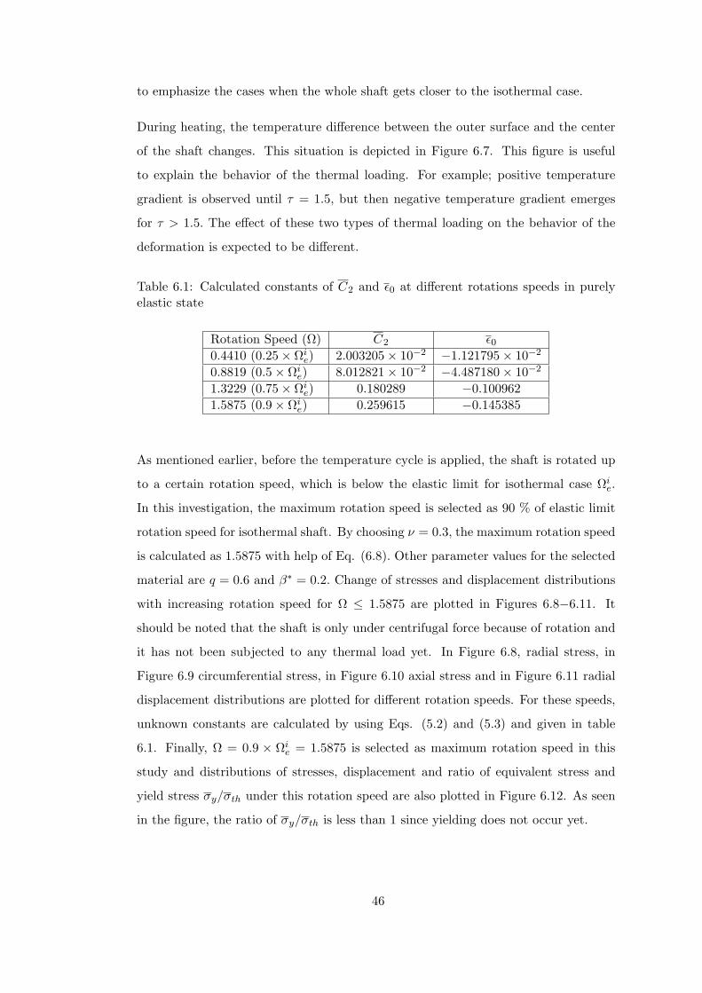
to emphasize the cases when the whole shaft gets closer to the isothermal case.

During heating, the temperature difference between the outer surface and the center

of the shaft changes. This situation is depicted in Figure 6.7. This figure is useful

to explain the behavior of the thermal loading. For example; positive temperature

gradient is observed until τ = 1.5, but then negative temperature gradient emerges

for τ > 1.5. The effect of these two types of thermal loading on the behavior of the

deformation is expected to be different.

Table 6.1: Calculated constants of C2 and ε0 at different rotations speeds in purelyelastic state

Rotation Speed (Ω) C2 ε00.4410 (0.25× Ωi

e) 2.003205× 10−2 −1.121795× 10−2

0.8819 (0.5× Ωie) 8.012821× 10−2 −4.487180× 10−2

1.3229 (0.75× Ωie) 0.180289 −0.100962

1.5875 (0.9× Ωie) 0.259615 −0.145385

As mentioned earlier, before the temperature cycle is applied, the shaft is rotated up

to a certain rotation speed, which is below the elastic limit for isothermal case Ωie.

In this investigation, the maximum rotation speed is selected as 90 % of elastic limit

rotation speed for isothermal shaft. By choosing ν = 0.3, the maximum rotation speed

is calculated as 1.5875 with help of Eq. (6.8). Other parameter values for the selected

material are q = 0.6 and β∗ = 0.2. Change of stresses and displacement distributions

with increasing rotation speed for Ω ≤ 1.5875 are plotted in Figures 6.8−6.11. It

should be noted that the shaft is only under centrifugal force because of rotation and

it has not been subjected to any thermal load yet. In Figure 6.8, radial stress, in

Figure 6.9 circumferential stress, in Figure 6.10 axial stress and in Figure 6.11 radial

displacement distributions are plotted for different rotation speeds. For these speeds,

unknown constants are calculated by using Eqs. (5.2) and (5.3) and given in table

6.1. Finally, Ω = 0.9 × Ωie = 1.5875 is selected as maximum rotation speed in this

study and distributions of stresses, displacement and ratio of equivalent stress and

yield stress σy/σth under this rotation speed are also plotted in Figure 6.12. As seen

in the figure, the ratio of σy/σth is less than 1 since yielding does not occur yet.

46

Distribution of temperature at constant time is time<timet

0.0

0.2

0.4

0.6

0.8

1.0

0.0 0.2 0.4 0.6 0.8 1.0

Non-dimensional radial coordinate

Non

-dim

ensi

onal

tem

pera

ture

2.1=τ

6.0=τ

2.0=τ

4.0=τ

8.0=τ

0.1=τ

Figure 6.2: Transient temperature field at τ ≤ 1.2

47

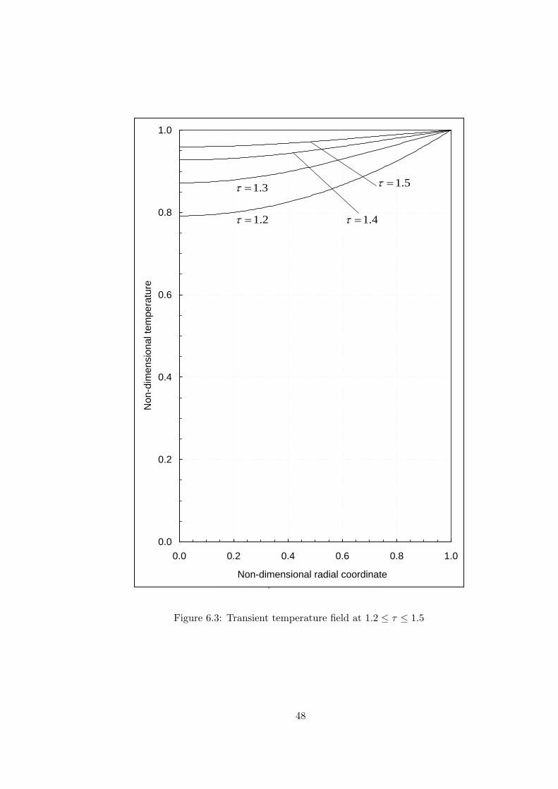
Distribution of temperature at constant time is time<timet

0.0

0.2

0.4

0.6

0.8

1.0

0.0 0.2 0.4 0.6 0.8 1.0

Non-dimensional radial coordinate

Non

-dim

ensi

onal

tem

pera

ture

2.1=τ

3.1=τ

4.1=τ

5.1=τ

Figure 6.3: Transient temperature field at 1.2 ≤ τ ≤ 1.5

48

Distribution of temperature at constant time is time<timet

0.0

0.2

0.4

0.6

0.8

1.0

0.0 0.2 0.4 0.6 0.8 1.0

Non-dimensional radial coordinate

Non

-dim

ensi

onal

tem

pera

ture

9.1=τ

3.2=τ

7.2=τ

5.1=τ

7.1=τ

5.2=τ

1.2=τ

Figure 6.4: Transient temperature field at 1.5 ≤ τ ≤ 2.7

49

Distribution of temperature at constant time is time<timet

0.0

0.2

0.4

0.6

0.8

1.0

0.0 0.2 0.4 0.6 0.8 1.0

Non-dimensional radial coordinate

Non

-dim

ensi

onal

tem

pera

ture

7.2=τ

0.3=τ

8.2=τ

9.2=τ

Figure 6.5: Transient temperature field at 2.7 ≤ τ ≤ 3.0

50

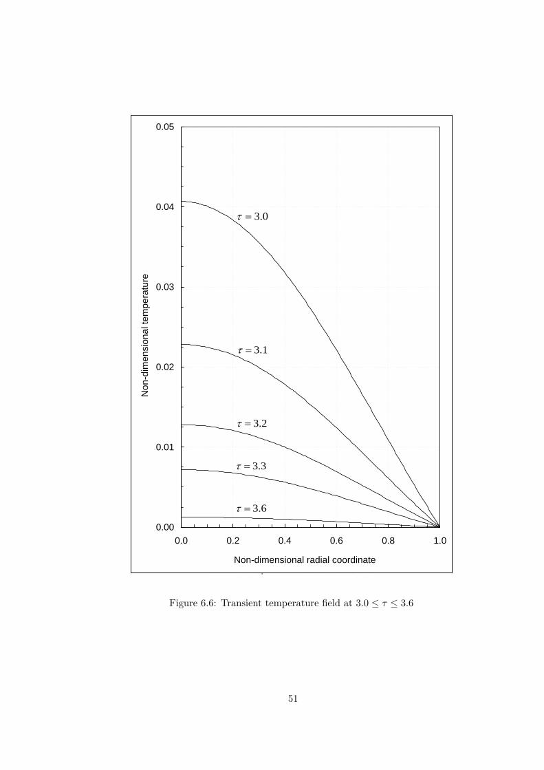
Distribution of temperature at constant time is time<timet

0.00

0.01

0.02

0.03

0.04

0.05

0.0 0.2 0.4 0.6 0.8 1.0

Non-dimensional radial coordinate

Non

-dim

ensi

onal

tem

pera

ture

0.3=τ

1.3=τ

2.3=τ

3.3=τ

6.3=τ

Figure 6.6: Transient temperature field at 3.0 ≤ τ ≤ 3.6

51

Distribution of temperature at constant time is time<timet

-0.3

-0.2

-0.1

0.0

0.1

0.2

0.3

0 1 2 3 4 5

Non-dimensional time

Tem

pera

ture

diff

eren

ce b

etw

een

oute

r sur

face

and

the

cent

er

tτ ct ττ + ct ττ +2

Figure 6.7: Change of temperature difference between outer surface and the center ofthe shaft with time

52

0.0

0.2

0.4

0.6

0.8

1.0

1.2

0.0 0.2 0.4 0.6 0.8 1.0

Non-dimensional radial coordinate

Non

-dim

ensi

onal

radi

al s

tress

ieΩ×=Ω 25.0

ieΩ×=Ω 5.0

ieΩ×=Ω 75.0

ieΩ×=Ω 9.0

Figure 6.8: Radial stress distribution in the shaft with increasing rotation speed

53

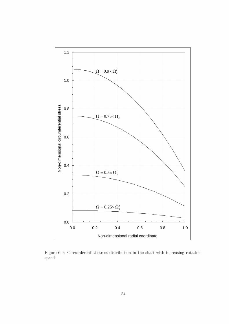
0.0

0.2

0.4

0.6

0.8

1.0

1.2

0.0 0.2 0.4 0.6 0.8 1.0

Non-dimensional radial coordinate

Non

-dim

ensi

onal

circ

umfe

rent

ial s

tress

ieΩ×=Ω 25.0

ieΩ×=Ω 5.0

ieΩ×=Ω 75.0

ieΩ×=Ω 9.0

Figure 6.9: Circumferential stress distribution in the shaft with increasing rotationspeed

54

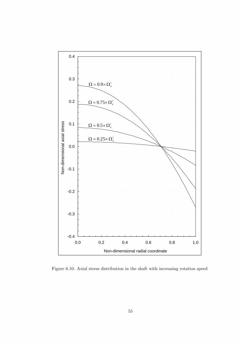
-0.4

-0.3

-0.2

-0.1

0.0

0.1

0.2

0.3

0.4

0.0 0.2 0.4 0.6 0.8 1.0

Non-dimensional radial coordinate

Non

-dim

ensi

onal

axi

al s

tress

ieΩ×=Ω 25.0

ieΩ×=Ω 5.0

ieΩ×=Ω 75.0

ieΩ×=Ω 9.0

Figure 6.10: Axial stress distribution in the shaft with increasing rotation speed

55

0.00

0.05

0.10

0.15

0.20

0.0 0.2 0.4 0.6 0.8 1.0

Non-dimensional radial coordinate

Non

-dim

ensi

onal

radi

al d

ispl

acem

ent

ieΩ×=Ω 25.0

ieΩ×=Ω 5.0

ieΩ×=Ω 75.0

ieΩ×=Ω 9.0

Figure 6.11: Radial displacement distribution in the shaft with increasing rotationspeed

56

-0.4

-0.2

0.0

0.2

0.4

0.6

0.8

1.0

1.2

0.0 0.2 0.4 0.6 0.8 1.0

Non-dimensional radial coordinate

Non

-dim

ensi

onal

stre

sses

and

dis

plac

emen

t

zσ

θσ

rσ

u

thy σσ /

Figure 6.12: Stresses and radial displacement distributions in purely elastic stateunder Ω = 0.9× Ωi

e = 1.5875

57

In the following calculations, rotation speed is fixed at Ω = 0.9 × Ωie = 1.5875 and

temperature cycle, which is described in Figure 6.1, is started to be applied. The next

step is to find the yielding time and the location where it initially starts. For this

reason, time is slowly increased in the temperature cycle and it is searched whether

the condition of σy = σth is reached. In Figure 6.13, distribution of σy/σth along the

radial direction at different times is presented. As seen in the figure, at τ = 0, which

is the beginning of the temperature cycle, this ratio is less than 1. As time passes, the

ratio decreases until around τ = 0.37. Then the ratio starts to increase dramatically.

When time reaches to τ = τp = 1.5519, which is shortly after the beginning of the

cooling time (τ = τt + τc = 1.5), σy/σth becomes equal to 1 at x = 0. It is observed

that the center of the shaft is a critical location for yielding. The evolution of the

ratio σy/σth with time at x = 0 is plotted in Figure 6.14. As seen in this figure, the

ratio decreases in the early stages until around τ = 0.37 as observed in Figure 6.13.

One observes that only after the onset of cooling at τ = 1.5 the temperature of the

inner parts of the shaft reaches its maximum. The corresponding reduction of the

yield stress σth leads to plasticization, which starts at the center. Hence, the last two

figures prove that plastic deformation emerges firstly at τ = τp = 1.5519 and on x = 0.

Table 6.2: Calculated constants of C2 and ε0 versus time in purely elastic state

Time (τ) C2 ε00.3 0.266619 −4.733532× 10−2

1.2 0.298012 0.3921731.35 0.300679 0.4295011.5 0.301720 0.444076

1.5519 (τp) 0.301329 0.438607

Elastic stresses and displacement for different time values prior to yielding (τ <

1.5519) are calculated after the determination of the corresponding integration con-

stants. These constants are presented in table 6.2. In Figures from 6.15 to 6.18,

radial stress, circumferential stress, axial stress and radial displacement distributions

at different time steps in τ < 1.5519 are presented, respectively. Finally, distributions

of stresses and radial displacement at τ = τp = 1.5519 is shown all together in Figure

6.19. It should be noted again that this figure is drawn at a time when yielding starts.

Hence, formulation of elastic-plastic state is used for τ > 1.5519 until unloaded state.

58

0.6

0.7

0.8

0.9

1.0

1.1

0.0 0.2 0.4 0.6 0.8 1.0Non-dimensional radial coordinate

Rat

io o

f equ

ival

ent s

tress

and

yie

ld s

tress

4.1=τ

5.1=τ3.1=τ

2.1=τ0.1=τ

0=τ

8.0=τ

6.0=τ

2.0=τ

4.0=τ

5519.1== pττ

Figure 6.13: Ratio of equivalent and yield stresses at different time until plastic flow

59

0.6

0.7

0.8

0.9

1.0

1.1

0.0 0.2 0.4 0.6 0.8 1.0 1.2 1.4 1.6

Non-dimensional time

Rat

io o

f equ

ival

ent s

tress

and

yie

ld s

tress

at t

he c

ente

r

5519.1== pττ

Figure 6.14: Change of ratio of equivalent and yield stresses with time until plasticflow at the center

60

0.0

0.1

0.2

0.3

0.4

0.5

0.6

0.7

0.8

0.9

1.0

1.1

1.2

1.3

0.0 0.2 0.4 0.6 0.8 1.0

Non-dimensional radial coordinate

Non

-dim

ensi

onal

radi

al s

tress

3.0=τ

2.1=τ

35.1=τ

5.1=τ

5519.1== pττ

Figure 6.15: Radial stress distribution at different time steps in purely elastic state

61

0.0

0.1

0.2

0.3

0.4

0.5

0.6

0.7

0.8

0.9

1.0

1.1

1.2

1.3

0.0 0.2 0.4 0.6 0.8 1.0

Non-dimensional radial coordinate

Non

-dim

ensi

onal

circ

umfe

rent

ial s

tress

3.0=τ

2.1=τ

35.1=τ

5.1=τ

5519.1== pττ

Figure 6.16: Circumferential stress distribution at different time steps in purely elasticstate

62

-0.6

-0.5

-0.4

-0.3

-0.2

-0.1

0.0

0.1

0.2

0.3

0.4

0.5

0.6

0.0 0.2 0.4 0.6 0.8 1.0

Non-dimensional radial coordinate

Non

-dim

ensi

onal

axi

al s

tress

3.0=τ

2.1=τ

35.1=τ

5.1=τ

5519.1== pττ

Figure 6.17: Axial stress distribution at different time steps in purely elastic state

63

0.0

0.1

0.2

0.3

0.4

0.5

0.6

0.7

0.8

0.9

0.0 0.2 0.4 0.6 0.8 1.0

Non-dimensional radial coordinate

Non

-dim

ensi

onal

radi

al d

ispl

acem

ent

3.0=τ

2.1=τ

35.1=τ5.1=τ

5519.1== pττ

Figure 6.18: Radial displacement distribution at different time steps in purely elasticstate

64

-0.5

-0.3

-0.1

0.1

0.3

0.5

0.7

0.9

1.1

1.3

0.0 0.2 0.4 0.6 0.8 1.0

Non-dimensional radial coordinate

Non

-dim

ensi

onal

stre

sses

and

dis

plac

emen

t

zσ

θσ

rσ

u

Figure 6.19: Stresses and radial displacement distributions in purely elastic state atτ = τp = 1.5519

65

As stated earlier, elastic-plastic state of stress is confined in the time interval τp <

τ < τub with onset of plasticization time τp and unloading bounding time τub being

critical time intervals to be determined. In order to determine τub, the condition that is

described in Eq. (5.21) is used. Evolution of plastic circumferential strain component

with respect to time is observed. In the shaft, there are three critical locations where

unloading may commence. These are center of the shaft x = 0, interface radius

between two plastic regions x = x1, and interface radius between plastic region II and

elastic region x = x2. Here, it should be noted that x1 and x2 are functions of time.

Evolutions of plastic circumferential strain component at x = 0 and x = x1(τ) are

plotted in Figure 6.20. Additionally, derivative of plastic circumferential strain with

respect to time is calculated by using forward difference as

dεpθ

dτ=

εpθ (τ + ∆τ)− εp

θ (τ)∆τ

, (6.9)

and plotted in Figure 6.21 using time increments of ∆τ = 0.005. As seen in these two

figures, plastic circumferential strain component increase first, then rate of the increase

slows down with time. For x = x1, increase in the strain ceases at τ = τub|x=x1=

1.8454, i.e., when the condition of (5.21) is satisfied. This time may be considered as

a possible starting time of unloaded state according to interface radius between two

plastic regions. However, unloading starts at the center at τ = τub|x=0 = 1.8469 as

followed in these figures. This shows that x1 is more critical radial coordinate than

the center of the shaft since unloading emerges earlier. Furthermore, the small time

difference of τub between these two points proves that movement of unloading from

interface radius x1 to the center is very fast.

On the other hand, another critical radial coordinate that is x = x2 should be exam-

ined for unloading condition. At this interface radius, plastic circumferential strain is

always zero because this radial coordinate is adjacent to the elastic region. Hence, it

is not possible to investigate the behavior of the plastic strains at this coordinate like

at x = 0 or x = x1. However, evolution of interface radius x2 with time gives some

hints to evaluate the behavior of the plastic strains around there. Evolution of x2(τ)

with time is plotted in Figure 6.22. Additionally, evolution of change in x2 with time

is obtained by forward difference, which is similar to the Eq. (6.9)

dx2 (τ)dτ

=x2 (τ + ∆τ)− x2 (τ)

∆τ, (6.10)

66

and plotted in Figure 6.23 by choosing ∆τ = 0.002. These two figures show that

when time reaches τ = 1.7882, expansion of x2 stops all of a sudden. This situation is

quite interesting since plastic region always moves into elastic region during loading.

Because of the termination in the expansion of plastic region II, plastic strains does not

increase at any radial coordinates beyond x2. Hence, condition of (5.21) is satisfied at

τ = 1.7882 and on x = 0.5707. Furthermore, this time value is earlier than those for

x = 0 and x = x1. Thus, we can discuss that unloading emerges at τ = τub = 1.7882

on x = 0.5707 and moves into plastic regions. Therefore, we have obtained the time

limits of elastic-plastic state.

Table 6.3: Calculated constants in elastic-plastic state at different time values

Time (τ) C1 C2 C3 C4 C5

1.5519 (τp) 0 0.301329 1.083954 0 01.57 1.556682× 10−5 0.301106 1.077291 0 4.246629× 10−3

1.6 9.963254× 10−5 0.300789 1.066483 0 1.226341× 10−2

1.66 3.467889× 10−4 0.300097 1.047876 0 2.649257× 10−2

1.72 5.436446× 10−4 0.299031 1.033410 0 3.590192× 10−2

1.7882 (τub) 6.473691× 10−4 0.297313 1.020649 0 4.118450× 10−2

Time (τ) C6 ε01.5519 (τp) 0 0.438607

1.57 1.054304× 10−6 0.4348271.6 6.492465× 10−6 0.4268671.66 2.245565× 10−5 0.4067891.72 3.529008× 10−5 0.38360

1.7882 (τub) 4.223217× 10−5 0.355186

Numerical results for the elastic-plastic state in time interval τp < τ < τub are pre-

sented in Figures 6.24−6.34. In Figure 6.24, stresses, radial displacement and the

ratio of equivalent and yield stresses are plotted at τ = τp = 1.5519, which is the

upper time limit of the purely elastic state and the lower time limit of the elastic-

plastic state. In the figure, while dots represent the results that are obtained with the

formulation of the purely elastic state, solid lines represent those of the elastic-plastic

state. As seen in the figure, these two results perfectly fit each other and this verifies

that formulations of the both states are correct. Thereafter, time instant is selected as

τ = 1.57, τ = 1.6, τ = 1.66, τ = 1.72 and τ = τub = 1.7882 to plot corresponding dis-

tributions of stresses and displacement in Figures 6.25−6.29, respectively. Similarly,

67

at these time instants, plastic strains are presented in Figures 6.30−6.34. The plastic

strains at τ = τub = 1.7882 are permanent plastic strains which will be used in the

unloaded state and are also presented in tabular form in Appendix D.2. Additionally,

the unknown integration constants that are calculated in elastic-plastic state are given

in table 6.3.

Evolution of the border radii in τp < τ < τub gives enough information about the

elastic-plastic behavior of the material under loading. This evolution with all regions

and critical time values, i.e., τp and τub, can be seen in Figure 6.35. This figure shows

that, at τ = τp = 1.5519 plastic regions I and II emerge simultaneously and spread

out (compare [12]). Up to τ = τub, the shaft consists of plastic region I at inner part,

plastic region II at the middle and elastic region at outer part. However, the expansion

of the plastic zone comes soon to an end, and at τ = τub = 1.7882 the plastic-elastic

border radius x2 attains a stationary value as explained with Figures 6.22 and 6.23.

At τ = τub = 1.7882, plastic strains that are seen in Figure 6.34, are frozen and the

quick expansion of an unloaded region is approximated by the assumption of sudden

unloading (indicated by the dashed line in Figure 6.35). Here xu separates plastic

regions and predeformed elastic region. That is, for τ > τub, the shaft consists of

predeformed elastic region, in the range 0 ≤ x ≤ xu2(= 0.5707) and elastic region in

the range xu2 ≤ x ≤ 1, and unloaded state will be valid in the whole shaft.

As discussed above, sudden unloading is approximated in this study. Error between

this approximation and exact unloading is negligibly small as shown in [38]. Further-

more, to estimate error thus introduced, Figure 6.36 depicts the ratio of the equivalent

stress σy and the yield stress σth versus time for three different radii, i.e., x = 0, x = 0.1

and x = x1 (τub) = 0.2324. One observes that the maximum violation of the yield

condition occurs at the center, but it is only about 0.3 %. Hence, one reasonably may

conclude that the stress distribution thus obtained is a very good approximation of

the true stress distribution.

68

0.000

0.005

0.010

0.015

0.020

0.025

1.5 1.6 1.7 1.8 1.9

Non-dimensional time

Non

-dim

ensi

onal

pla

stic

tang

entia

l stra

in

0=x

5519.1=pτ

8469.10=

=xubτ

8454.11=

=xxubτ

)(1 τxx =

Figure 6.20: Evolutions of plastic tangential strain component with time at x = 0 andx = x1

69

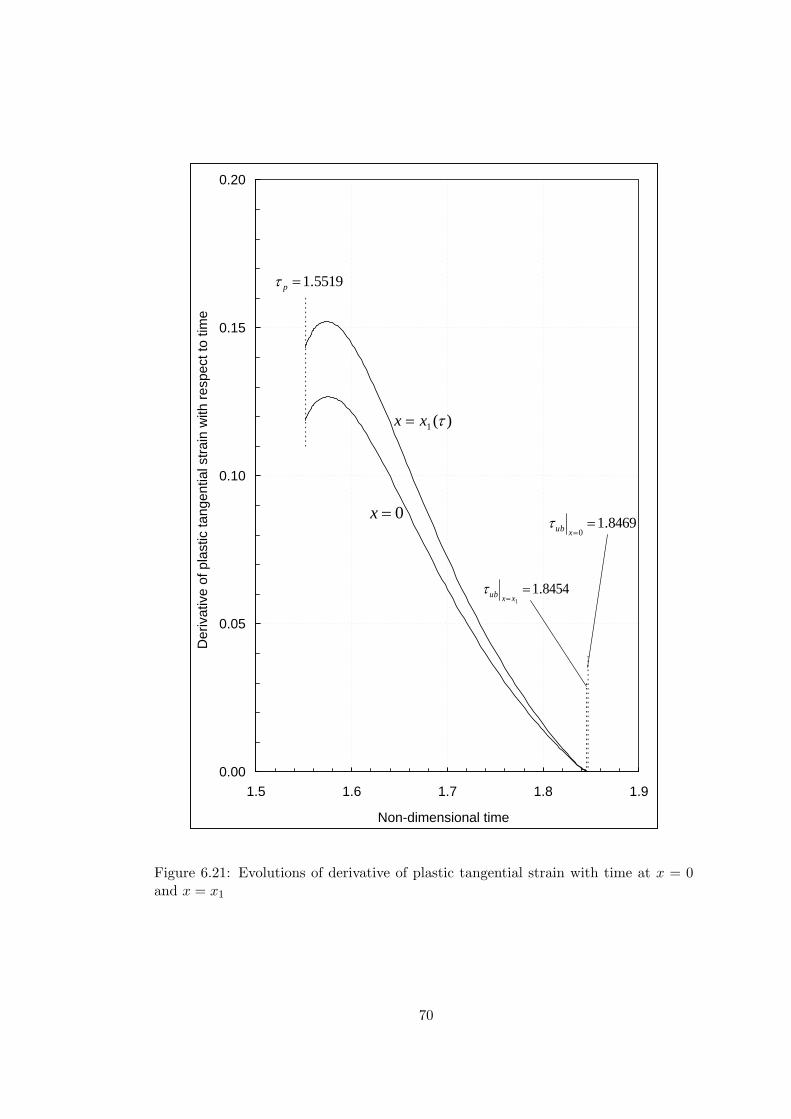
0.00

0.05

0.10

0.15

0.20

1.5 1.6 1.7 1.8 1.9

Non-dimensional time

Der

ivat

ive

of p

last

ic ta

ngen

tial s

train

with

resp

ect t

o tim

e

0=x

5519.1=pτ

8469.10=

=xubτ

8454.11=

=xxubτ

)(1 τxx =

Figure 6.21: Evolutions of derivative of plastic tangential strain with time at x = 0and x = x1

70

1.50

1.55

1.60

1.65

1.70

1.75

1.80

1.85

0.0 0.2 0.4 0.6 0.8 1.0Non-dimensional radial coordinate

Non

-dim

ensi

onal

tim

e

7882.1=ubτ

5707.02 =x

5519.1=pτ

)(2 τxx =

Figure 6.22: Evolution of interface radius x2 with time

71

0

10

20

30

40

50

60

70

80

90

100

1.5 1.6 1.7 1.8 1.9

Non-dimensional time

Der

ivat

ive

of x

2 with

resp

ect t

o tim

e

7882.1=ubτ

Figure 6.23: Evolution of derivative of x2 with respect to time

72

-0.4

-0.2

0.0

0.2

0.4

0.6

0.8

1.0

1.2

0.0 0.2 0.4 0.6 0.8 1.0Non-dimensional radial coordinate

Non

-dim

ensi

onal

stre

sses

and

dis

plac

emen

t

zσ

θσ

rσ

u

thy σσ /

Figure 6.24: Stresses and radial displacement distributions in elastic-plastic state atτ = τp = 1.5519

73

-0.4

-0.2

0.0

0.2

0.4

0.6

0.8

1.0

1.2

0.0 0.2 0.4 0.6 0.8 1.0

Non-dimensional radial coordinate

Non

-dim

ensi

onal

stre

sses

and

dis

plac

emen

t

1005.01 =x

2601.02 =x

zσ

θσ

rσ

u

thy σσ /

Figure 6.25: Stresses and radial displacement distributions in elastic-plastic state atτ = 1.57

74

-0.4

-0.2

0.0

0.2

0.4

0.6

0.8

1.0

1.2

0.0 0.2 0.4 0.6 0.8 1.0

Non-dimensional radial coordinate

Non

-dim

ensi

onal

stre

sses

and

dis

plac

emen

t

1571.01 =x 3989.02 =x

zσ

θσ

rσ

u

thy σσ /

Figure 6.26: Stresses and radial displacement distributions in elastic-plastic state atτ = 1.6

75

-0.4

-0.2

0.0

0.2

0.4

0.6

0.8

1.0

1.2

0.0 0.2 0.4 0.6 0.8 1.0

Non-dimensional radial coordinate

Non

-dim

ensi

onal

stre

sses

and

dis

plac

emen

t

2075.01 =x 5157.02 =x

zσ

θσ

rσ

u

thy σσ /

Figure 6.27: Stresses and radial displacement distributions in elastic-plastic state atτ = 1.66

76

-0.4

-0.2

0.0

0.2

0.4

0.6

0.8

1.0

1.2

0.0 0.2 0.4 0.6 0.8 1.0

Non-dimensional radial coordinate

Non

-dim

ensi

onal

stre

sses

and

dis

plac

emen

t

2266.01 =x 5586.02 =x

zσ

θσ

rσ

u

thy σσ /

Figure 6.28: Stresses and radial displacement distributions in elastic-plastic state atτ = 1.72

77

-0.4

-0.2

0.0

0.2

0.4

0.6

0.8

1.0

1.2

0.0 0.2 0.4 0.6 0.8 1.0

Non-dimensional radial coordinate

Non

-dim

ensi

onal

stre

sses

and

dis

plac

emen

t

2324.01 =x 5707.02 =x

zσ

θσ

rσ

u

thy σσ /

Figure 6.29: Stresses and radial displacement distributions in elastic-plastic state atτ = τub = 1.7882

78

-0.04

-0.03

-0.02

-0.01

0.00

0.01

0.02

0.03

0.0 0.2 0.4 0.6 0.8 1.0

Non-dimensional radial coordinate

Non

-dim

ensi

onal

pla

stic

stra

ins

1005.01 =x

2601.02 =x

prε

pθε

pzε

Figure 6.30: Plastic strain distributions in elastic-plastic state at τ = 1.57

79

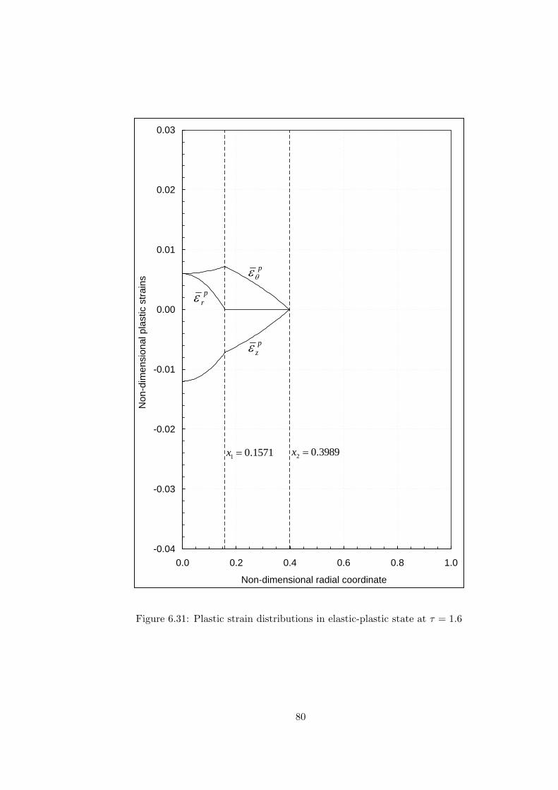
-0.04

-0.03

-0.02

-0.01

0.00

0.01

0.02

0.03

0.0 0.2 0.4 0.6 0.8 1.0

Non-dimensional radial coordinate

Non

-dim

ensi

onal

pla

stic

stra

ins

1571.01 =x 3989.02 =x

prε

pθε

pzε

Figure 6.31: Plastic strain distributions in elastic-plastic state at τ = 1.6

80

-0.04

-0.03

-0.02

-0.01

0.00

0.01

0.02

0.03

0.0 0.2 0.4 0.6 0.8 1.0

Non-dimensional radial coordinate

Non

-dim

ensi

onal

pla

stic

stra

ins

2075.01 =x 5157.02 =x

prε

pθε

pzε

Figure 6.32: Plastic strain distributions in elastic-plastic state at τ = 1.66

81

-0.04

-0.03

-0.02

-0.01

0.00

0.01

0.02

0.03

0.0 0.2 0.4 0.6 0.8 1.0

Non-dimensional radial coordinate

Non

-dim

ensi

onal

pla

stic

stra

ins

2266.01 =x 5586.02 =x

prε

pθε

pzε

Figure 6.33: Plastic strain distributions in elastic-plastic state at τ = 1.72

82

-0.04

-0.03

-0.02

-0.01

0.00

0.01

0.02

0.03

0.0 0.2 0.4 0.6 0.8 1.0

Non-dimensional radial coordinate

Non

-dim

ensi

onal

pla

stic

stra

ins

2324.01 =x 5707.02 =x

prε

pθε

pzε

Figure 6.34: Plastic strain distributions in elastic-plastic state at τ = τub = 1.7882

83

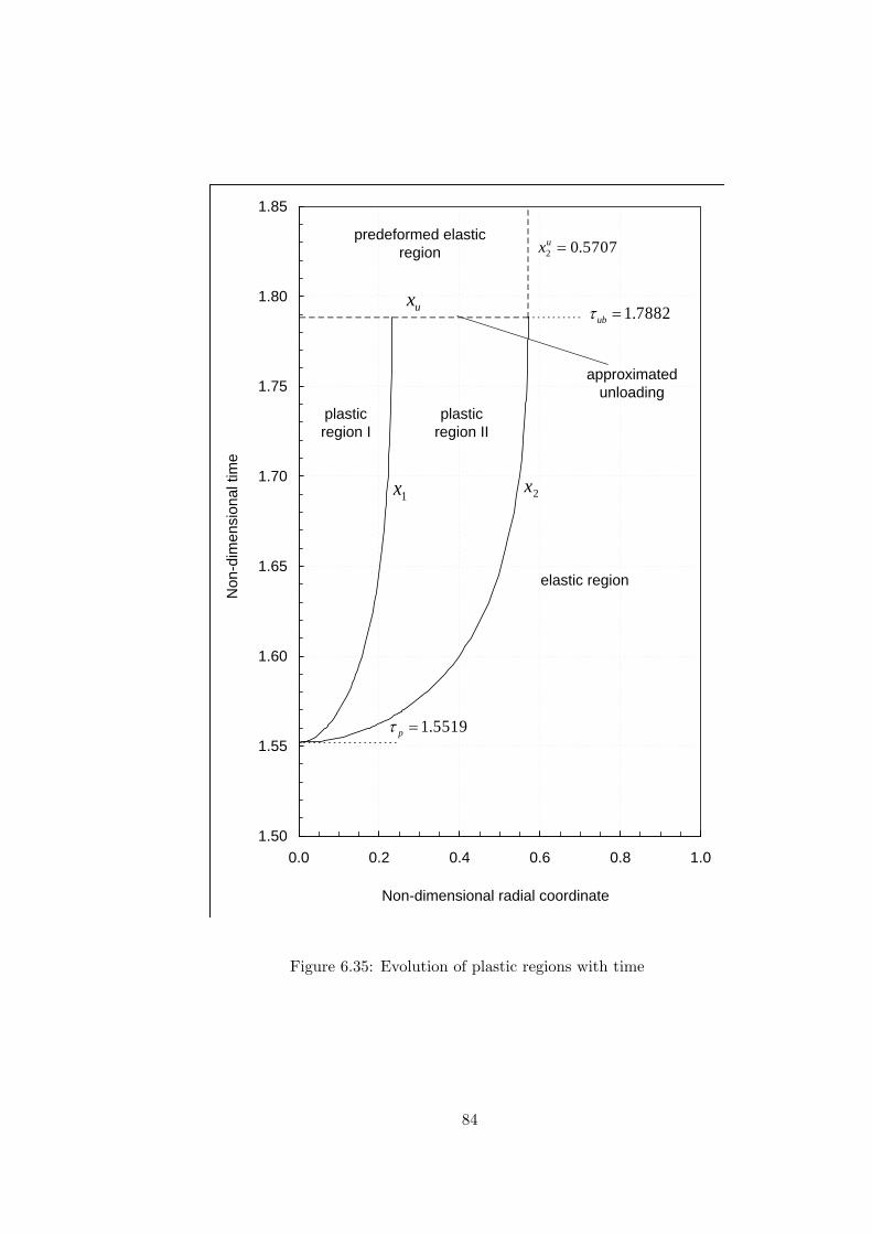
1.50

1.55

1.60

1.65

1.70

1.75

1.80

1.85

0.0 0.2 0.4 0.6 0.8 1.0

Non-dimensional radial coordinate

Non

-dim

ensi

onal

tim

e

1x 2x

plastic region I

plastic region II

elastic region

predeformed elastic region

7882.1=ubτ

5519.1=pτ

ux

approximated unloading

5707.02 =ux

Figure 6.35: Evolution of plastic regions with time

84

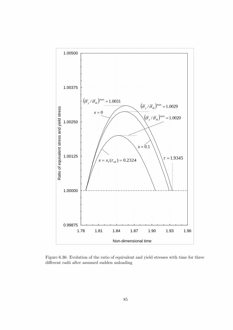
0.99875

1.00000

1.00125

1.00250

1.00375

1.00500

1.78 1.81 1.84 1.87 1.90 1.93 1.96

Non-dimensional time

Rat

io o

f equ

ival

ent s

tress

and

yie

ld s

tress

9345.1=τ

1.0=x

0=x

2324.0)(1 == ubxx τ

( ) 0031.1/ max =thy σσ( ) 0029.1/ max =thy σσ

( ) 0020.1/ max =thy σσ

Figure 6.36: Evolution of the ratio of equivalent and yield stresses with time for threedifferent radii after assumed sudden unloading

85

To observe stresses and displacement in unloaded state at 1.7882 < τ < 2.7, Figures

from 6.37 to 6.42 are plotted. Response variables are calculated at the upper time

limit of elastic-plastic state and at the beginning time of the unloaded state, τ =

τub = 1.7882, and drawn in Figure 6.37. In the figure, dots represents the results

of the elastic-plastic state, and solid lines are those of unloaded state. As seen in

the figure, fairly good agreement between two results is obtained. This verifies that

the formulations of the both states are correct. Moreover, in Figure 6.38, time is

selected as τ = 1.9 to present corresponding distributions of stresses and displacement.

Between Figures 6.39 and 6.42, 0.2 time increments are used to plot distributions of

the response variables. In the last figure, which is plotted at time instant τ = 2.7, the

temperature cycle ends and the surface temperature returns to reference temperature.

In this cooling time interval, it is visible from the figures that stresses and especially

displacement decrease dramatically with time after unloading starts. Additionally, it

should be remained that plastic strains for these time instants are the same as those

given in Figure 6.34. For these figures, the non-dimensional unknown constants C∗2

and ε0 are calculated with help of Eqs. (5.24−5.25) and the results are presented in

Table 6.4.

Table 6.4: Calculated constants in unloaded state at different time values until theend of the temperature cycle

Time (τ) C∗2 ε0

1.7882(τub) 0.304070 0.3551861.9 0.300530 0.3056252.1 0.293728 0.2103952.3 0.286692 0.1118952.5 0.279583 1.236726× 10−2

2.7 0.272450 −8.748429× 10−2

It certainly takes time to reach homogeneous temperature distribution in the whole

shaft after reaching reference temperature of the outer surface as followed in Figure

6.6. Hence, until isothermal case is obtained, stresses and displacement in the shaft

can vary with time at any point. These distributions are plotted for following time

values: τ = 3.0 in Figure 6.43, τ = 3.6 in Figure 6.44, τ = 4.0 in Figure 6.45, τ = 10.0

in Figure 6.46, and τ = 20.0 in Figure 6.47. As seen, there are not any differences

86

between Figure 6.46 and Figure 6.47. This shows that when time reaches to τ = 20.0,

the shaft behaves isothermal. Then thermal load is removed totally from the shaft.

Integration constants that are obtained to plot Figures from 6.43 to 6.47 are presented

in Table 6.5.

Table 6.5: Calculated constants in unloaded state at different time values after thetemperature cycle

Time (τ) C∗2 ε0

3.0 0.268744 −0.1393793.6 0.268014 −0.1495884.0 0.267993 −0.14988410.0 0.267991 −0.14991620.0 0.267991 −0.149916

An interesting result is observed on the evolution of stresses and radial displacement

with time at some critical locations, i.e., the center (x = 0) and the outer surface

(x = 1) of the shaft. In Figure 6.48, the evolution of the radial stress at the center

with time is presented. In the figure, the critical time values, i.e., the end of the heating

time τt, the beginning of the cooling time τt+τc, the end of the cooling time 2τt+τc, the

time when plastic flow starts τp and the time when unloaded state starts τub, separate

the time intervals. As seen in the figure, the stress tends to vary at each time interval in

different manner. The radial stress at the center initially increases during the surface

heating process (τ ≤ τt). On the other hand, it dramatically decreases with different

slopes at the time interval when the surface temperature remains constant and in

the cooling time interval (τt ≤ τ ≤ 2τt + τc). When the outer surface temperature

reaches back to the reference temperature at τ = 2τt + τc, the radial stress starts to

increase again. However, the stress tends to a certain value, which is σr = 1.1043,

with increasing time since the rotation speed is constant and the isothermal case is

approaching. This value is higher than the initial one (at τ = 0) and this proves that

some residual stresses remain in the shaft because of the temperature field. It should

also be noted that this evolution is the same as the evolution of circumferential stress

at the center since σr = σθ at this location.

87

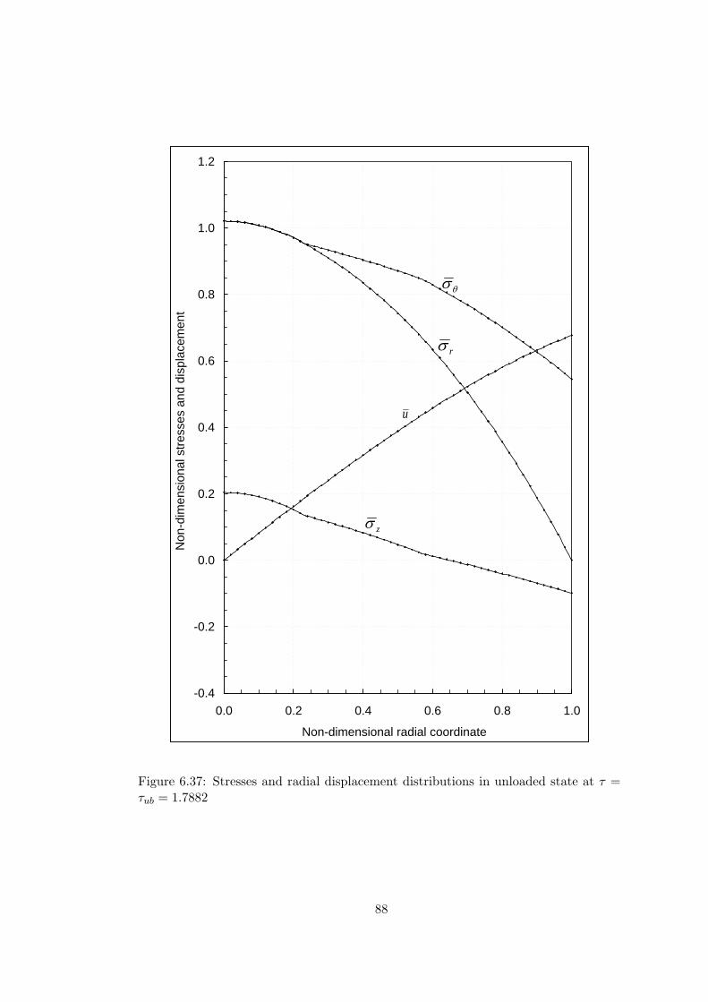
-0.4

-0.2

0.0

0.2

0.4

0.6

0.8

1.0

1.2

0.0 0.2 0.4 0.6 0.8 1.0

Non-dimensional radial coordinate

Non

-dim

ensi

onal

stre

sses

and

dis

plac

emen

t

zσ

θσ

rσ

u

Figure 6.37: Stresses and radial displacement distributions in unloaded state at τ =τub = 1.7882

88

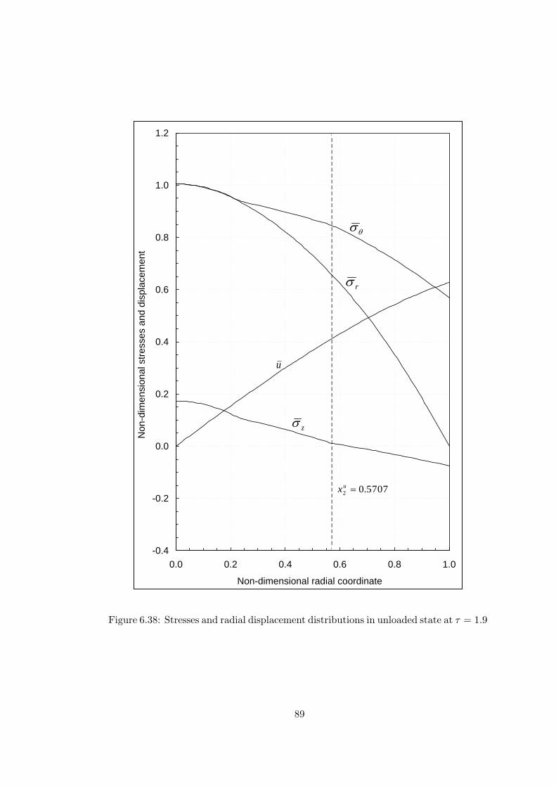
-0.4

-0.2

0.0

0.2

0.4

0.6

0.8

1.0

1.2

0.0 0.2 0.4 0.6 0.8 1.0

Non-dimensional radial coordinate

Non

-dim

ensi

onal

stre

sses

and

dis

plac

emen

t

zσ

θσ

rσ

u

5707.02 =ux

Figure 6.38: Stresses and radial displacement distributions in unloaded state at τ = 1.9

89

-0.4

-0.2

0.0

0.2

0.4

0.6

0.8

1.0

1.2

0.0 0.2 0.4 0.6 0.8 1.0

Non-dimensional radial coordinate

Non

-dim

ensi

onal

stre

sses

and

dis

plac

emen

t

zσ

θσ

rσ

u

5707.02 =ux

Figure 6.39: Stresses and radial displacement distributions in unloaded state at τ = 2.1

90

-0.4

-0.2

0.0

0.2

0.4

0.6

0.8

1.0

1.2

0.0 0.2 0.4 0.6 0.8 1.0

Non-dimensional radial coordinate

Non

-dim

ensi

onal

stre

sses

and

dis

plac

emen

t

zσ

θσ

rσ

u

5707.02 =ux

Figure 6.40: Stresses and radial displacement distributions in unloaded state at τ = 2.3

91

-0.4

-0.2

0.0

0.2

0.4

0.6

0.8

1.0

1.2

0.0 0.2 0.4 0.6 0.8 1.0

Non-dimensional radial coordinate

Non

-dim

ensi

onal

stre

sses

and

dis

plac

emen

t

zσ

θσ

rσ

u

5707.02 =ux

Figure 6.41: Stresses and radial displacement distributions in unloaded state at τ = 2.5

92

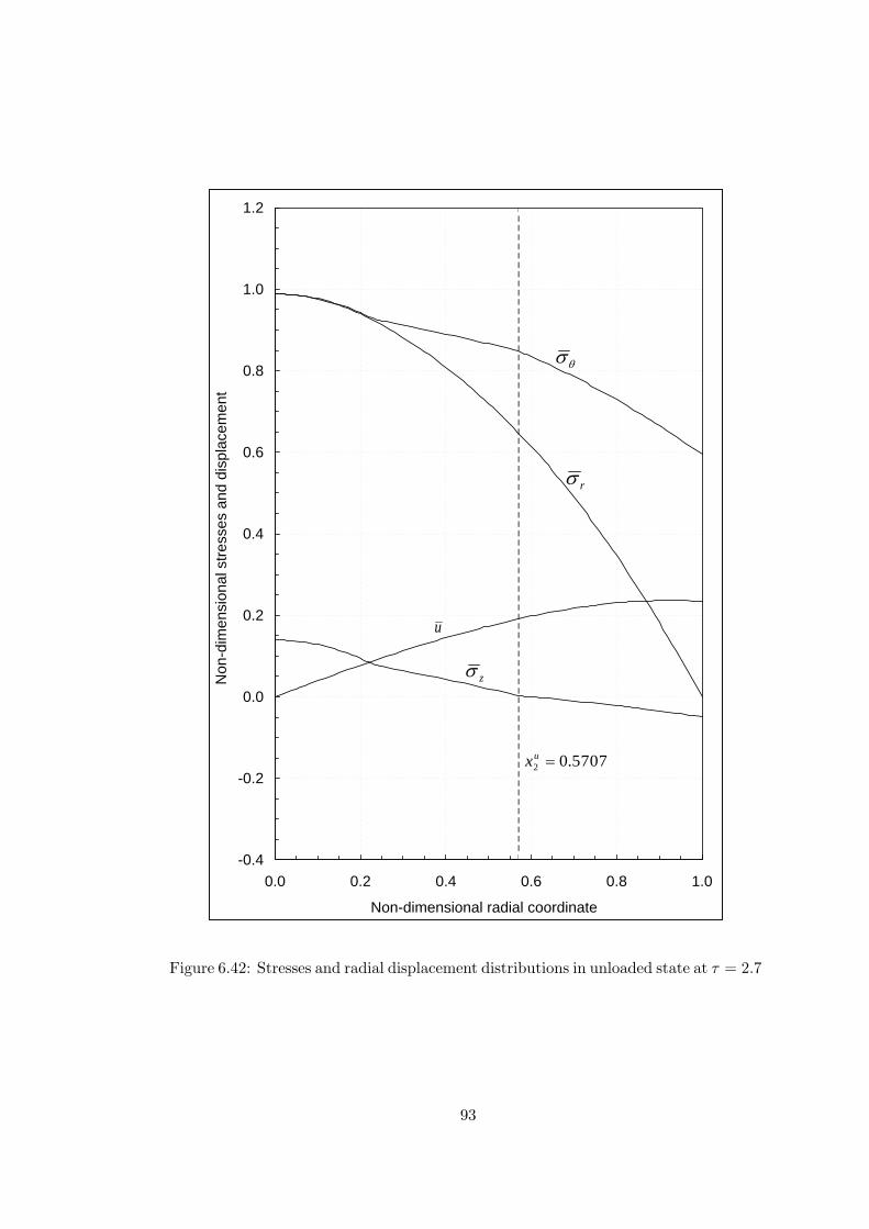
-0.4

-0.2

0.0

0.2

0.4

0.6

0.8

1.0

1.2

0.0 0.2 0.4 0.6 0.8 1.0

Non-dimensional radial coordinate

Non

-dim

ensi

onal

stre

sses

and

dis

plac

emen

t

zσ

θσ

rσ

u

5707.02 =ux

Figure 6.42: Stresses and radial displacement distributions in unloaded state at τ = 2.7

93

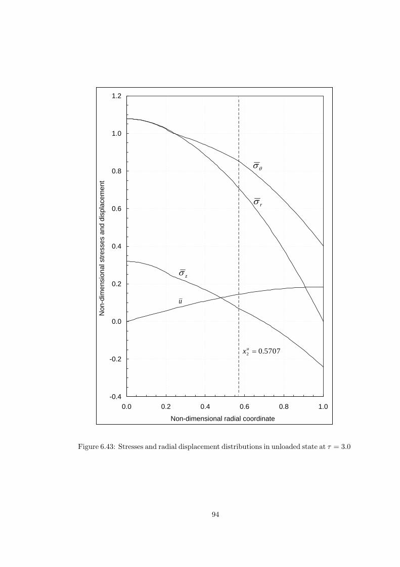
-0.4

-0.2

0.0

0.2

0.4

0.6

0.8

1.0

1.2

0.0 0.2 0.4 0.6 0.8 1.0

Non-dimensional radial coordinate

Non

-dim

ensi

onal

stre

sses

and

dis

plac

emen

t

zσ

θσ

rσ

u

5707.02 =ux

Figure 6.43: Stresses and radial displacement distributions in unloaded state at τ = 3.0

94

-0.4

-0.2

0.0

0.2

0.4

0.6

0.8

1.0

1.2

0.0 0.2 0.4 0.6 0.8 1.0

Non-dimensional radial coordinate

Non

-dim

ensi

onal

stre

sses

and

dis

plac

emen

t

zσ

θσ

rσ

u

5707.02 =ux

Figure 6.44: Stresses and radial displacement distributions in unloaded state at τ = 3.6

95

-0.4

-0.2

0.0

0.2

0.4

0.6

0.8

1.0

1.2

0.0 0.2 0.4 0.6 0.8 1.0

Non-dimensional radial coordinate

Non

-dim

ensi

onal

stre

sses

and

dis

plac

emen

t

zσ

θσ

rσ

u

5707.02 =ux

Figure 6.45: Stresses and radial displacement distributions in unloaded state at τ = 4.0

96

-0.4

-0.2

0.0

0.2

0.4

0.6

0.8

1.0

1.2

0.0 0.2 0.4 0.6 0.8 1.0

Non-dimensional radial coordinate

Non

-dim

ensi

onal

stre

sses

and

dis

plac

emen

t

zσ

θσ

rσ

u

5707.02 =ux

Figure 6.46: Stresses and radial displacement distributions in unloaded state at τ =10.0

97

-0.4

-0.2

0.0

0.2

0.4

0.6

0.8

1.0

1.2

0.0 0.2 0.4 0.6 0.8 1.0

Non-dimensional radial coordinate

Non

-dim

ensi

onal

stre

sses

and

dis

plac

emen

t

5707.02 =x

zσ

θσ

rσ

u

Figure 6.47: Stresses and radial displacement distributions in unloaded state at τ =20.0

98

0.95

1.00

1.05

1.10

1.15

1.20

1.25

0 1 2 3 4 5

Non-dimensional time

Non

-dim

ensi

onal

radi

al s

tress

at t

he c

ente

r

ct ττ +

tτ ct ττ +2

pτ

ubτ

Figure 6.48: Evolution of the radial stress at the center of the shaft

99

In Figure 6.49, the evolution of the circumferential stress at the surface of the shaft

is presented. The behavior of the circumferential stress at x = 1 is the opposite of

that at x = 0. In Figures 6.50 and 6.51, the evolution of axial stresses at the center

and the outer surface are plotted, respectively. These two figures show that adverse

behavior is observed at the center and the outer surface for the axial stress. Lastly,

the evolution of the radial displacement component at the outer surface of the shaft

is presented in Figure 6.52. The displacement increases with the superposition of the

rotation and the surface heating until τ = τt + τc. However, it decreases during the

cooling of the outer surface and becomes constant at u = 0.1719.

As seen in Figures from 6.48 to 6.52, some differences occur between the beginning and

the end of the thermal process for stresses (σi|τ=5 − σi|τ=0) and radial displacement

(u|τ=5 − u|τ=0) because of the residual effects. These differences are calculated and

presented in Table 6.6. As seen in the table, the maximum difference is observed in

the axial stress at the center of the shaft. However, differences in the other stresses

and radial displacement are very small.

Table 6.6: Differences in response variables between the beginning and the end of thethermal process

σr(0)|τ=5 − σr(0)|τ=0 = 0.024259,

σθ(1)|τ=5 − σθ(1)|τ=0 = 0.002590,

σz(0)|τ=5 − σz(0)|τ=0 = 0.101247,

σz(1)|τ=5 − σz(1)|τ=0 = −0.011005,

u(1)|τ=5 − u(1)|τ=0 = 0.002266.

During the unloaded state, the ratio of the equivalent and the yielding stresses should

be less than 1. To observe this, the distribution of σy/σth on radial direction for

different times is presented in Figure 6.53. This ratio decreases with time since the

thermal effect slowly disappears and thus the isothermal case is obtained. Finally,

when the time approaches to nearly or higher value than τ = 5.0, the ratio of σy/σth

remains constant in the whole shaft. Furthermore, Figure 6.54 shows the evolution of

ratio of equivalent and yield stresses with increasing time at the center of the shaft.

It should be noted that at τ ≈ 1.9 the ratio of σy/σth is higher than 1. The reason for

this overlap is the approximated unloading and is described in Figure 6.36.

100

For completeness, the stresses after stand-still are shown on Figure 6.55. The distri-

butions of stresses are plotted at τ = 20.0 and for Ω = 0. In other words, the thermal

effect is far away and the rotation is stopped. Hence, these stresses are called residual

stresses that remain in the shaft because of the thermal and the mechanical loading.

As can be seen from the figure, secondary plastic flow does not occur.

In Figure 6.56, Tresca’s yield conditions are presented in the usual way as Tresca’s

hexagon in the deviatoric plane of the three-dimensional stress space. These figures

show four phases of the development of the plastic flow occurring in a rotating solid

shaft under unsteady thermal load. Figure 6.56.a is sketched at τ = τp. As seen,

yielding occurs when the stress image point at x = 0 reaches an edge regime of the

Tresca’s hexagon in principal stress space. Additionally, x = x1 and x = x2 are also

seem at the same point at the onset of the yielding. At this time, outer part of the

shaft is still elastic then remaining part of the stress space is on the inside of the

hexagon. With increasing time, for which τp < τ < τub, x2 moves on the one side of

Tresca’s hexagon according to yield condition (see also Figure 2.2) as seen in Figure

6.56.b. Stress field onto deviatoric plane of the principal stress space at τ = τub and

for τ > τub are given in Figures 6.56.c and 6.56.d, respectively. As seen in Figure

6.56.d, the stress space is on the inside of the hexagon since the secondary yielding

does not occur during unloading.

In Figure 6.57, the evolution of the elastic and the plastic regions are summarized

by sketching them at the cross-section of the shaft. The evolution of the regions at

different times are plotted respectively. The evolution starts with the purely elastic

state at τ = τp = 1.5519 and for Ω = 0.9×Ωie = 1.5875 as seen in Figure 6.57.a. Only

elastic region appears in the figure. Additionally, at this time, plastic flow starts,

too and moves to the outer zone of the shaft with the increasing time as seen in the

Figures from 6.57.b to 6.57.l. In these figures, all regions are drawn with different

shapes to make a distinction among the evolution of them. At τ = τub = 1.7882, the

unloading starts and then the predeformed elastic region remains on the inner zone

of the shaft as seen in Figures from 6.57.m to Figure 6.57.o. In the last one, all loads

have been removed, i.e., rotation is stopped in the isothermal shaft.

101

0.0

0.1

0.2

0.3

0.4

0.5

0.6

0.7

0 1 2 3 4 5

Non-dimensional time

Non

-dim

ensi

onal

tang

entia

l stre

ss o

n th

e ou

ter s

urfa

ce

ct ττ +

tτ ct ττ +2pτ

ubτ

Figure 6.49: Evolution of the tangential stress on the outer surface of the shaft

102

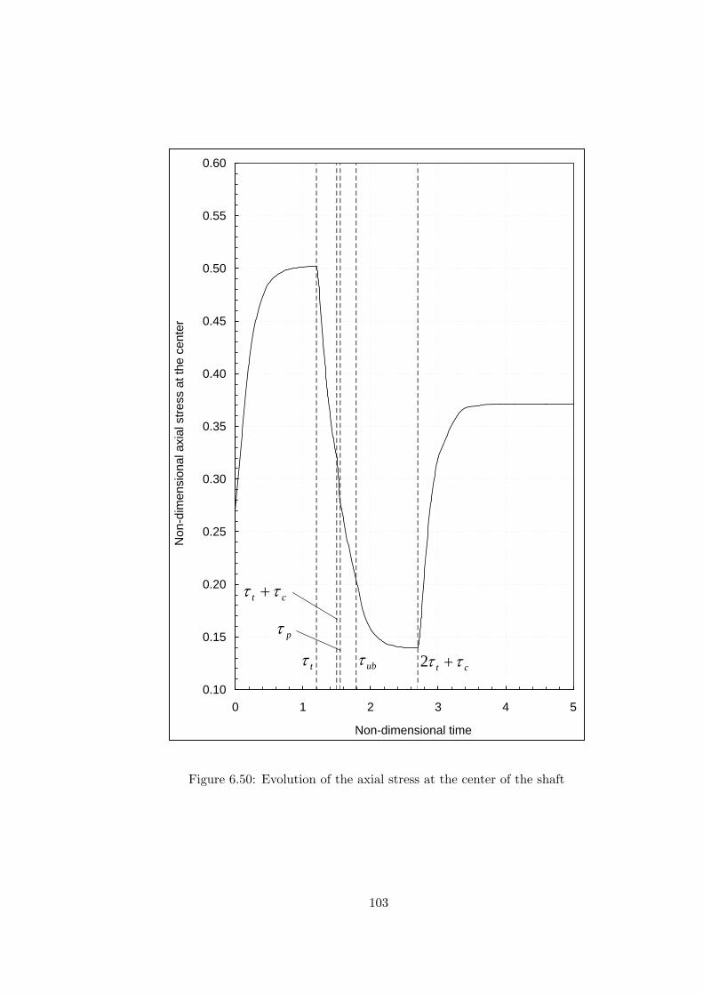
0.10

0.15

0.20

0.25

0.30

0.35

0.40

0.45

0.50

0.55

0.60

0 1 2 3 4 5

Non-dimensional time

Non

-dim

ensi

onal

axi

al s

tress

at t

he c

ente

r

ct ττ +

tτ ct ττ +2

pτ

ubτ

Figure 6.50: Evolution of the axial stress at the center of the shaft

103

-0.6

-0.5

-0.4

-0.3

-0.2

-0.1

0.0

0 1 2 3 4 5

Non-dimensional time

Non

-dim

ensi

onal

axi

al s

tress

on

the

oute

r sur

face

ct ττ +

tτ ct ττ +2

pτ

ubτ

Figure 6.51: Evolution of the axial stress on the outer surface of the shaft

104

0.0

0.2

0.4

0.6

0.8

1.0

0 1 2 3 4 5

Non-dimensional time

Non

-dim

ensi

onal

radi

al d

ispl

acem

ent o

n th

e ou

ter s

urfa

ce

ct ττ +

tτ ct ττ +2pτ

ubτ

Figure 6.52: Evolution of the radial displacement on the outer surface of the shaft

105

0.6

0.7

0.8

0.9

1.0

1.1

0.0 0.2 0.4 0.6 0.8 1.0

Non-dimensional radial coordinate

Rat

io o

f equ

ival

ent s

tress

and

yie

ld s

tress

7882.1== ubττ

1.2=τ

3.2=τ

5.2=τ

7.2=τ

8.2=τ

0.3=τ

0.5=τ

Figure 6.53: Ratio of equivalent and yield stresses at different time in the unloadedstate

106

0.60

0.70

0.80

0.90

1.00

1.10

1.7 2.2 2.7 3.2 3.7 4.2 4.7

Non-dimensional time

Rat

io o

f equ

ival

ent s

tress

and

yie

ld s

tress

at t

he c

ente

r

ct ττ +2ubτ

Figure 6.54: Change of ratio of equivalent and yield stresses at the center with timein the unloaded state

107

-0.10

-0.05

0.00

0.05

0.10

0.15

0.0 0.2 0.4 0.6 0.8 1.0

Non-dimensional radial coordinate

Non

-dim

ensi

onal

resi

dual

stre

sses

0rσ

0θσ

0zσ

Figure 6.55: Approximate residual stress distribution at stand-still (Ω = 0) aftercooling

108

0=x

2xx =

1=x

1=x1=x

1xx =0=x

1=x2xx =

1xx =0=x

2xx =1xx =

0=x

rσ

θσθσ zσzσ

rσrσ

θσθσ zσzσ

rσ)(a )(b

)(c )(d

Figure 6.56: Stress field in the rotating shaft mapped onto the deviatoric plane of theprincipal stress space (sketch) at (a) τ = τp, (b) τp < τ < τub, (c) τ = τub, (d) τ > τub

109

Figure 6.57: Evolution of elastic, plastic and predeformed elastic regions on the crosssection of the shaft at different times

110

6.3 Summary and Discussion

The closed form solution to a rotating solid shaft with the temperature dependent yield

stress under a temperature cycle is presented. The shaft is subjected to a centrifugal

force due to the rotation and an unsteady-state thermal load due to temperature

cycle, i.e., the temperature of its surface is increased slowly and linearly with time,

held constant for some time, and then decreased linearly with time to its reference

temperature. Thermally induced wave phenomena is vanished since the thermal load

is applied slowly. Elastic-plastic state of stress is presumed to obey Tresca’s yield

criterion and the associated flow rule with it. Furthermore, state of generalized plane

strain and circular symmetry are considered.

The earlier studies, which are related to the present thesis, are separated into three cat-

egories. In the first category, the investigations which include elastic or elastic-plastic

solutions of the cylindrical machine elements that are subjected to solely rotation are

presented. The second category consists of the analysis for the non-rotating cylindrical

elements under only thermal load. Investigation of the deformation due to superposi-

tion of these two loads on a disk or shaft are presented under title of the third category.

The literature review shows the requirement of the theoretical investigation for the

problem of an elastic-plastic rotating solid shaft, which is one of the most wide-spread

machine parts, under unsteady thermal load, in which interesting and unpredictable

results may be expected.

Initially, the entire shaft is presumed to be in a purely elastic state. As soon as

the yielding condition is satisfied, two different plastic regions emerge at the center

of the shaft, simultaneously. They expand into the elastic region in time until an

elastic unloading occurs at the plastic-elastic interface radius. Next, plastic regions

do not move into elastic region anymore. On the other hand, the predeformed elastic

region spreads rapidly into the plastic zone. For the mathematical model of this

elastic-plastic behavior, the governing equations and their analytical solutions for

these regions are obtained with the help of the basic equations. These solutions may

include unknown integration constants, axial strain and the interface radii. To evaluate

each unknown value in the purely elastic state, elastic-plastic state and approximated

unloaded state, boundary and interface conditions are used. The analytical expressions

111

for the calculation of integration constants are also derived. The rest of the unknowns

are calculated numerically. Finally, numerical results of the problem for the chosen

parameters are presented.

112

CHAPTER 7

CONCLUSION

First, for certain combinations of the parameter values a qualitatively different be-

havior, such as partial or full plasticization, may occur by depending on the loading

conditions. Nevertheless, the results which are presented in Section 6.2 may be con-

sidered characteristic for a wide class of the shafts under similar conditions.

Secondly, starting at the center, the plasticization may occur even in the shafts which

have been designed purely elastic. Remarkably, at least if pronounced temperature

gradients occur, this happens only after the temperature of the surface has started to

decrease again. The delay in the beginning of the plasticization and hence also in the

beginning of the unloading may be attributed to the inhomogeneity of the temperature

field.

Additionally, from the engineering point of view, the stress distribution after com-

plete cooling and stand-still is of particular interest. It can be concluded that, all of

these residual stresses are small as compared to yield limit. Remarkably, the resid-

ual stresses, after stand-still, with any smaller angular speed remain far beyond the

secondary yield limit. As a further interesting result, the axial stress in the centre is

found to be dominating one.

Finally, it should be pointed out that prior to unloading the numerical effort essentially

is restricted to the solution of an algebraic system of equations; if the proposed ap-

proximate calculation of the stresses after unloading is applied, in the later stages only

numerical integrations must be added. As the error introduced by the approximation

is very small, significant benefits by applying much more complex purely numerical

methods like FE-codes are hardly to be expected.

113

REFERENCES

[1] Timoshenko S., Goodier J.N.: Theory of Elasticity, 3rd ed., New York: McGraw-Hill (1970).

[2] Rees D.W.A.: The Mechanics of Solids and Structures, New York: McGraw Hill(1990).

[3] Ugural A.C., Fenster S.K.: Advanced Strength and Applied Elasticity, 2nd ed.,Amsterdam: Elsevier (1975).

[4] Boley B.A, Weiner J.H.: Theory of Thermal Stresses, 1st ed., p. 246. New York:Wiley Press (1960).

[5] Faupel J.H., Fisher F.E.: Engineering Design, 2nd ed., pp. 29-30. New York:Wiley (1981).

[6] Nadai A.: Theory of Flow and Fracture of Solids vol.1, 2nd ed., New York:McGraw Hill (1950).

[7] Davis E.A., Conelly F.M.: Stress distribution and plastic deformation in rotatingcylinders of strain-hardening material. Journal of Applied Mechanics of the ASME26, 25-30 (1959).

[8] Hodge Jr.P.G., Balaban M.: Elastic-plastic analysis of a rotating cylinder. Inter-national Journal of Mechanical Science 4, 465-476 (1962).

[9] Lenard J., Haddow J.B.: Plastic collapse speeds for rotating cylinders. Interna-tional Journal of Mechanical Sciences 14, 285-292 (1972).

[10] Gamer U., Sayir M.: Elastic-plastic stress distribution in a rotating solid shaft.Journal of Applied Mathematics and Physics (ZAMP) 35, 601-617 (1984).

[11] Gamer U., Mack W., Varga I.: Rotating elastic-plastic solid shaft with fixed ends.International Journal of Engineering Science 35, 253-267 (1997).

[12] Mack W.: The rotating elastic-plastic solid shaft with free ends. TechnischeMechanik 12, 119-124 (1991).

[13] Lindner T., Mack W.: Residual stresses in an elastic-plastic shaft with fixedends after previous rotation. The Journal of Applied Mathematics and Mechanics(ZAMM) 78, 75-86 (1998).

[14] Gamer U., Lance R.H.: Stress distribution in a rotating elastic-plastic tube. ActaMechanica 50, 1-8 (1983).

[15] Mack W.: Rotating elastic-plastic tube with free ends. International Journal ofSolids and Structures 27, 1461-1476 (1991).

114

[16] Mack W.: Entlastung und sekundares Fließen in rotierenden elastisch-plastischenHohlzylindern. The Journal of Applied Mathematics and Mechanics (ZAMM) 72,65-68 (1992).

[17] Guven U.: Elastic-plastic stress distribution in a rotating hyperbolic disk withrigid inclusion. International Journal of Mechanical Sciences 40, 97-109 (1998).

[18] Eraslan A.N., Orcan Y.: On the rotating elastic-plastic solid disks of variablethickness having concave profiles. International Journal of Mechanical Sciences44, 1445-1466 (2002).

[19] Eraslan A.N., Argeso H.: Limit angular velocities of variable thickness rotatingdisks. International Journal of Solids and Structures 39, 3109-3130 (2002).

[20] Eraslan A.N., Stress distributions in elastic-plastic rotating disks with ellipticalthickness profiles using Tresca and Von Mises criteria. The Journal of AppliedMathematics and Mechanics (ZAMM) 85, 1-15 (2005).

[21] Eraslan A.N.: On the linearly hardening rotating solid shaft. European Journalof Mechanics A/Solids 22, 295-307 (2003).

[22] Eraslan A.N.: Von Mises’ yield criterion and nonlinearly hardening rotatingshafts. Acta Mechanica 168, 129-144 (2004).

[23] Eraslan A.N., Mack W.: A computational procedure for estimating residualstresses and secondary plastic flow limits in nonlinearly strain hardening rotatingshafts. Forschung Im Ingenieurwesen/Engineering Research 69, 65-75 (2005).

[24] Horgan C.O., Chan A.M.: The stress response of functionally graded isotropiclinearly elastic rotating disks. Journal of Elasticity 55, 219-230 (1999).

[25] Eraslan A.N., Akis T.: On the plane strain and plane stress solutions of func-tionally graded rotating solid shaft and solid disk problems. Acta Mechanica 181,43-63 (2006).

[26] Akis T., Eraslan A.N.: The stress response and onset of yield of rotating FGMhollow shafts. Acta Mechanica 187, 169-187 (2006).

[27] Eraslan A.N., Akis, T.: The stress response of partially plastic rotating FGMhollow shafts: analytical treatment for axially constrained ends. Mechanics BasedDesign of Structures and Machines 34, 241-260 (2006).

[28] Eraslan A.N., Arslan E.: Plane strain analytical solutions to rotating partiallyplastic graded hollow shafts. Turkish Journal of Engineering and EnvironmentalSciences 31, 273-287 (2007).

[29] Akis T., Eraslan A.N.: Exact solution of rotating FGM shaft problem in theelastoplastic state of stress. Archive of Applied Mechanics 77, 745-765 (2007).

[30] Dahl O.G.C.: Temperature and stress distribution in hollow cylinders. AmericanSociety of Mechanical Engineering Transactions 46, 161-208 (1924).

[31] Weiner J.H., Huddleston J.V.: Transient and residual stresses in heat-treatedcylinders. Journal of Applied Mechanics of the ASME 26, 31-39 (1959).

115

[32] Johnson W., Mellor P.B.: Plasticity for Mechanical Engineers, Great Britain: D.Van Nostrand Comp. (1970).

[33] Landau H.G., Zwicky E.E.Jr.: Transient and residual thermal stresses in anelastic-plastic cylinder. Journal of Applied Mechanics of the ASME 27, 481-488(1960).

[34] Mendelson A.: Plasticity: Theory and Application, 1st ed., New York: MscmillanComp. (1968).

[35] Chu S.C.: A numerical thermoelastic solution of a thick-walled tube. AmericanInstitute of Aeronautics and Astronautics (AIAA) Journal 12, 176-179 (1974).

[36] Perzyna P., Sawczuk A.: Problems of Thermoplasticity. Nuclear Engineering andDesign 24, 1-55 (1973).

[37] Ishikawa H.: A thermoelastoplastic solution for a circular solid cylinder subjectedto heating and cooling. Journal of Thermal Stresses 1, 211-222 (1978).

[38] Mack W., Gamer U.: Zur Berechnung der Restspannungen beim Abkuhlen ther-misch beanspruchter elastisch-plastischer Bauteile. Forschung im Ingenieurwe-sen/Engineering Research 54, 48-52 (1988).

[39] Jahanian S., Sabbaghian M.: Thermoelastoplastic and residual stresses in a hol-low cylinder with temperature-dependent properties. Journal of Pressure VesselTechnology 112, 85-91 (1990).

[40] Valentin R.A., Carey J.J: Thermal stresses and displacements in finite, heat-generating circular cylinders. Nuclear Engineering and Design 12, 277-290 (1970).

[41] Citakoglu E.: Thermal stresses in a finite rod with uniform energy generation un-der special BCs. METU Journal of Pure and Applied Sciences 9, 167-187 (1976).

[42] Citakoglu E., Eren N.: Thermal stresses in a finite composite cylinder with uni-form energy generation under special boundary conditions. METU Journal ofPure and Applied Sciences 12, 91-125 (1979).

[43] Orcan Y., Gamer U.: Elastic-plastic deformation of a centrally heated cylinder.Acta Mechanica 90, 61-80 (1991).

[44] Orcan Y.: Thermal stresses in a heat generating elastic-plastic cylinder with freeends. International Journal of Engineering Science 32, 883-898 (1994).

[45] Gulgec M., Orcan Y.: Elastic-plastic deformation of a heat generating tube withtemperature-dependent yield stress. International Journal of Engineering Science38, 89-106 (2000).

[46] Orcan Y., Gulgec M.: Elastic-plastic deformation of a tube with free ends sub-jected to internal energy generation. Turkish Journal of Engineering and Envi-ronmental Sciences 25, 601-610 (2001).

[47] Orcan Y., Eraslan A.N.: Thermal stresses in elastic-plastic tubes withtemperature-dependent mechanical and thermal properties. Journal of ThermalStresses 24, 1097-1113 (2001).

116

[48] Eraslan A.N.: Thermally induced deformations of composite tubes subjected toa nonuniform heat source. Journal of Thermal Stresses 26, 167-193 (2003).

[49] Eraslan A.N., Orcan Y.: Thermoplastic response of a linearly hardening cylindersubjected to nonuniform heat source and convective boundary condition. Me-chanics Based Design of Structures and Machines 32, 133–164 (2004).

[50] Eraslan A.N., Argeso H.: Computer solutions of plane strain axisymmetric ther-momechanical problems. Turkish Journal of Engineering and Environmental Sci-ences 29, 369-381 (2005).

[51] Argeso H., Eraslan A.N.: On the use of temperature-dependent physical proper-ties in thermomechanical calculations for solid and hollow cylinders. InternationalJournal of Thermal Sciences 47, 136–146 (2008).

[52] Alujevic A., Legat J., Zupec J.: Thermal yield of a rotating hyperbolic disk. TheJournal of Applied Mathematics and Mechanics (ZAMM) 73, T283-T287 (1993).

[53] Alujevic A., Les P., Zupec J.: Plasticity of a thermally loaded rotating hyperbolicdisk. The Journal of Applied Mathematics and Mechanics (ZAMM) 73, T287-T290 (1993).

[54] Parmaksizoglu C., Guven U.: Plastic stress distribution in a rotating disk withrigid inclusion under a radial temperature gradient. Mechanical Structures andMachines 26, 9-20 (1998).

[55] Tarn J.Q.: Exact solutions for functionally graded anisotropic cylinders subjectedto thermal and mechanical loads. International Journal of Solids and Structures38, 8189-8206 (2001).

[56] Mack W., Plochl M.: Transient heating of a rotating elastic-plastic shrink fit.International Journal of Engineering Science 38, 921-938 (2000).

[57] Mack W., Plochl M., Gamer U.: Auswirkungen eines Temperaturzyklus aufeinen rotierenden elastisch-plastischen Querpreßverband mit vollem Einschluß.The Journal of Applied Mathematics and Mechanics (ZAMM) 81, S351-S352(2001).

[58] Eraslan A.N., Akis T.: On the elastic–plastic deformation of a rotating disksubjected to a radial temperature gradient. Mechanics Based Design of Structuresand Machines 31, 529-561 (2003).

[59] Eraslan A.N., Arslan E., Mack W.: The strain hardening rotating hollow shaftsubject to a positive temperature gradient. Acta Mechanica 194, 191-211 (2007).

[60] Arslan E., Mack W., Eraslan A.N.: The rotating elastic-plastic hollow shaftconveying a hot medium. Forschung im Ingenieurwesen/Engineering Research(to appear).

[61] Beer F.P., Johnston E.R., DeWolf J.T.: Mechanics of Materials, 3rd ed., NewYork: McGraw Hill (1943).

[62] Hill R.: The Mathematical Theory of Plasticity, London: Oxford University Press(1950).

117

[63] Von Mises R.: Mechanik der festen Koerper in Plastisch deformablem Zustand,Gottinger Nachrichten Math. Phys. Klasse 1, 582-592 (1913).

[64] Tresca H.: Memoire sur I’ecoulement des Corps Solides. Mem. Sci. Savants Acad.Sci. 18, 733-799 (1868).

[65] Chen W.F., Han D.J.: Plasticity for Structural Engineers. New York: Springer(1988).

[66] Saint-Venant B.: Memoire sur I’etablissement des equations differentielles desmouvements interieurs operes dans les corpse solides ductiles au dela des limitesou I’elasticite pourrait les ramener a leur premier etat. Comptes Rendus 70, 473-480 (1870).

[67] Levy M.: Memoire sur les equations generales des mouvements interieurs descorps solides ductile au dela limites ou I’elasticite purrait les ramener a leurpremier etat. Comptes Rendus 70, 1323-1325 (1870).

[68] Prandtl L.: Spannungsverteilung in plastischen Koerpern. 1st InternationalCongress on Applied Mechanics, Delft, 43-54 (1925).

[69] Reuss E.: Berueckesichtigung der elastischen Formaenderungen in der Plastiz-itaetstheorie. The Journal of Applied Mathematics and Mechanics (ZAMM) 10,266-274 (1930).

[70] Melan E.: Zur Plastizitat des raumlichen Kontinuus. Ingenieur-Archiv 9, 116-(1938).

[71] Carslaw H.S., Jaeger J.C.: Conduction of Heat in Solids, 2nd ed., pp. 201. Oxford:Clarendon Press (1959).

[72] Kreyszig E.: Advanced Engineering Mathematics, 8th ed., New York: Wiley Press(1999).

[73] Ziegler F.: Technische Mechanik der festen und flussigen Korper. Dritte, verb.Aufl., Ch. 4.3. Wien: Springer (1998).

[74] Mack W.: Spannungen im thermisch gefugten elastisch-plastischen Querpreßver-band mit elastischer Entlastung. Ingenieur-Archiv 56, 301-313 (1986).

[75] More J.J., Garbow B.S., Hillstrom K.E.: Testing unconstrained optimizationsoftware. ACM Transactions on Mathematical Software 7, 17-41 (1981).

[76] Davis J.D., Rabinowitz P.: Numerical Integration, 1st ed., Massachusetts: Blais-dell (1967).

118

APPENDIX A

DESCRIPTION OF FORTRAN CODES

Integration constants, axial strain, interface radii, analytical and numerical integrals,

and Bessel and hypergeometric functions are calculated by using Fortran 77 codes.

In the codes, non-dimensional and normalized variables and equations are used. The

codes are divided into three categories since three states of stress, which are purely

elastic state, elastic-plastic state and unloaded state, are examined in the study.

The first category includes Fortran codes for the purely elastic state (see Appendix

B). All codes in Appendix B (Appendices B1−B6) are compiled and run in the same

project since the main program is connected to the other subroutines and functions

by common block or dummy arguments. The main program in the first category is

called Purely Elastic State (see Appendix B.1). In this program, after the introduction

of the input parameters, unknown non-zero constants are calculated (with the help

of Eqs. (5.2) and (5.3) in dimensional form) and substituted into analytical expres-

sions of response variables (Eqs. (4.22)−(4.25)) at different radial coordinates. By

manipulating the non-dimensional time value, different distribution of the response

variables are obtained. During all these calculations, temperature distribution and a

temperature integral are calculated for each time and radial coordinate by using the

subroutine called Temperature Distribution (See Appendix B.2). In the subroutine,

the temperature and some integrals are superposed according to time interval by using

Eqs. (3.11). This subroutine takes the temperature and its integral by the connections

to the Fortran functions called Temperature (Appendix B.3) and Temperature Integral

1 (Appendix B.4). The first function calculates the non-dimensional temperature dis-

tribution given Eq. (3.9) and the second one calculates an exact temperature integral,

which is given in Eq. (4.20). Furthermore, the summation of the series in these tem-

119

perature equations are computed by using Fortran functions Series 1 (Appendix B.5)

and Series 2 (Appendix B.6). The Bessel functions and roots that appear in these

series may be computed by any Fortran subroutine. This subroutine calculates roots

of the zeroth order Bessel functions of the first kind γn according to Eq. (3.10) and,

the zeroth and the first order Bessel functions of the first kind J0 and J1. However,

this subroutine is not presented here. Finally, by executing the main program and the

connected five Fortran subroutines and functions, the response variables on the purely

elastic state are calculated and written into an output data file. For continuity of the

process, the instant time value is increased slowly by hand. However, the usage of

these subroutines are valid until a time value when the yielding conditions are satisfied

(Eq. (4.29)). After this certain time value, this codes become out of use since plastic

flow starts. For the following time values, the codes, which are written for the second

category, should be executed.

In the second category, Fortran codes for the numerical results of the elastic-plastic

state are considered. To calculate the results in this state, beside the codes presented

in Appendix C, those in Appendices B2−B6 are performed simultaneously. The main

program in this category is called Elastic Plastic state (Appendix C.1). This program

is designed to initially calculate six integration constants (C1−C6) analytically; then,

to compute three unknowns (ε0, r1 and r2) numerically (since a non-linear equation

system is obtained for the border radii) and lastly, to figure out the response vari-

ables in the elastic-plastic state. Analytical expressions for six integration constants

are placed into subroutine NLNEQN (Appendix C.2). Moreover, this subroutine in-

cludes interface and boundary conditions (Eqs. (5.9), (5.10) and (5.14)) to compute

the remaining unknowns. To compute these unknowns, subroutine HYBRD1, which

is implemented in the program called MINPACK is performed. The Fortran pro-

gram MINPACK is a non-linear equation system solver which uses the Powell Hybrid

Method (see [75]). The connection between the main program and Minpack is pro-

vided by NLNEQN. After the calculation of the all unknowns, the response variables

are obtained by making use of the subroutines Plastic Region I, Plastic Region II and

Elastic Region (Appendices C.3−C.5). These subroutines include analytical expres-

sions for three regions. The main program executes these subroutines for different

radial coordinates and writes the results in an output data file. Similar to first codes

120

category, the temperature distribution, the first temperature integral and summation

of the first two series are calculated by using the codes given in Appendices B2−B6 in

this codes category, too. Additionally, Fortran function Temperature Integral 2 (Ap-

pendix C.6) is performed to calculate temperature integrals in Eqs. (4.76) and (4.82).

The summation of the series in these equations are calculated with the help of function

Series 3 (Appendix C.7). Unlike others, these integral equations include hypergeo-

metric functions and these functions are calculated by using the Fortran codes called

Hypergeometric Function (Appendix C.8). The Fortran codes in the second category

may be used until the time when unloading conditions (Eq. (5.21)) are observed in the

results. For the following time values, the codes of third category, which are prepared

for the unloaded state, should be run.

The third category of the codes is used to calculate response variables in unloaded

state. The Fortran codes used in this category in addition to codes in Appendix

B.2−B.6 are presented in Appendix D. The main program called Unloaded State (see

Appendix D.1) is executed with codes above mentioned, namely, Temperature Dis-

tribution, Temperature, Temperature Integral 1, Series 1 and Series 2 . The main

program is arranged to calculate two non-zero unknown constants (C∗2 and ε0) with

the help of Eqs. (5.24) and (5.25) and to substitute these constants into analytical

expressions of response variables. In this process, it is necessary to access the values of

permanent plastic strains (εpri ) seen in the equations in the Chapter 4.5. The perma-

nent plastic strains are the ones which are computed in the program of Elastic-plastic

state (with the second category of the codes) at a time when the unloading starts.

Hence, the codes in the second category are run one more time and the calculated

plastic strains are written into a data file. The tabulated form of this data file, which

is called Permanent Plastic Strains, for the prescribed input parameters is given in

Table D.1 in Appendix D.2. The main program calls this file as an input. In the

calculations of the unlaoded state, we need to calculate some integral which include

the permanent plastic strains as given below.

INTEPS1 =∫ r

0

εprr − εpr

θ

ξdξ, (A.1)

INTEPS2 =∫ r

0ξ(εprr + εpr

θ

)dξ. (A.2)

The numerical integrations of these discrete permanent strain values are performed by

121

the Fortran program DAVINT efficiently. DAVINT, which is documented completely

in SC-M-69-335, integrates a function tabulated at arbitrarily space abscissas. This

Fortran program is the adapted and modified (by Rondall E. Jones) form of AVINT,

which is prepared by Davis and Rabinowitz [76]. Finally, all of these codes with the

input data file are executed for different time values and the response variables are

written into output data file for the unloaded state.

122

APPENDIX B

FORTRAN CODES OF PURELY ELASTIC STATE

B.1 MAIN PROGRAM: PURELY ELASTIC STATE

PROGRAM PURELY ELASTIC STATEC ----------C PURPOSE:C ----------C This program calculates the non-dimensional response variables inC the purely elastic state for the problem of rotating solid shaftC subjected to temperature cycle. All calculations are done forC non-dimensional parameters. Input parameters, which are describedC below, are initially introduced. Then non-zero integrationC constant C2 and axial strain EPS0 are calculated by using theC analytical expressions. Substituting the parameters and constantsC into the response variable leads to obtain output values at N1C radial points in the shaft. Results are printed to the output file,C which is titled ’A-ELAST.DAT’.C The program is connected to subroutine ’DISTRIBUTION’ to callC TBAR and INT1. Subroutine ’DISTRIBUTION’ is used to calculate someC integrals which include temperature terms. By substituting variableC R and the upper limits of the integral, INT1 is calculatedC analytically by using this subroutine. Additionally, thisC subroutine is also used to get TBAR which is non-dimensionalC temperature distribution.CC -----------------------C CONNECTED SUBROUTINESC -----------------------C 1) DISTRIBUTION (R, TBAR, ULIM, INT1, POW, INT2E).CC ----------------------------C DESCRIPTION OF PARAMETERS:C ----------------------------C INPUT:C BETA : Non-dimensional temperature dependence parameter ofC the material.C NU : Poisson’s ratio.C N1 : Number of data points in the shaft.C OMEGA : Non-dimensional angular velocity.C Q : A non-dimensional measure for the maximum surface

123

C temperature during the transient heating.C R : Non-dimensional radial coordinate.C TAU : Non-dimensional instant time.C TAUT : The non-dimensional time value when surface heatingC ends.C TAUC : The non-dimensional time value that the surfaceC temperature is held constant at maximum temperatureC value.CC OUTPUT:C C2 : Non-zero, non-dimensional integration constantC EPS0 : Non-dimensional axial strain.C SIGR : Non-dimensional radial stress component.C SIGT : Non-dimensional circumferential stress component.C SIGZ : Non-dimensional axial stress component.C SIGTHER : Non-dimensional yield stress.C SIGY : Non-dimensional equivalent stress.C U : Non-dimensional radial displacement component.C

IMPLICIT NONEINTEGER I, N1DOUBLE PRECISION TBAR, R, TAU, TAUT, TAUC, ULIM, TBARINT, TERM1,1 NU, Q, OMEGA, C2, DR, TERM2,2 SIGR, SIGT, SIGZ, U, BETA, SIGTHER, EPS0, SIGY,3 INT1, M, POW, INT2ECOMMON /PROP/ BETA, NU, Q, OMEGA, M, TAUT, TAUC, TAU

COPEN (61, FILE=’A-ELAST.DAT’)

CC -----------------------------------C MECHANICAL AND THERMAL PROPERTIESC -----------------------------------

NU = 0.3D0Q = 0.6D0BETA = 0.2D0

CC ------------------C ANGULAR VELOCITYC ------------------C The angular velocity is calculated as 90% of elastic limitC rotation speed for isothermal shaft.C

OMEGA = DSQRT(8.0*(1.0D0 - NU)/(3.0D0 - 4.0*NU))*0.9D0CC -----------------C TIME PARAMETERSC -----------------

TAU = 1.55194075D0TAUT = 1.2D0TAUC = 0.3D0

CC -----------C CONSTANTSC -----------C The unknown constants are calculated analytically. Subroutine

124

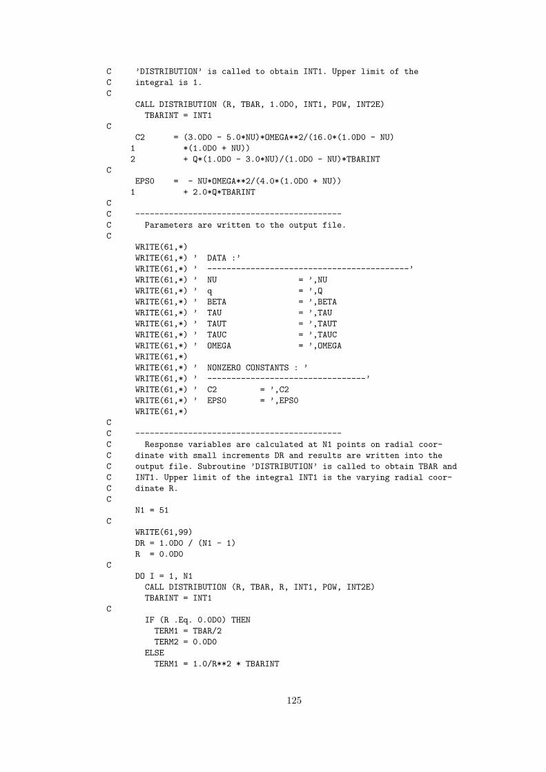
C ’DISTRIBUTION’ is called to obtain INT1. Upper limit of theC integral is 1.C

CALL DISTRIBUTION (R, TBAR, 1.0D0, INT1, POW, INT2E)TBARINT = INT1

CC2 = (3.0D0 - 5.0*NU)*OMEGA**2/(16.0*(1.0D0 - NU)1 *(1.0D0 + NU))2 + Q*(1.0D0 - 3.0*NU)/(1.0D0 - NU)*TBARINT

CEPS0 = - NU*OMEGA**2/(4.0*(1.0D0 + NU))1 + 2.0*Q*TBARINT

CC -------------------------------------------C Parameters are written to the output file.C

WRITE(61,*)WRITE(61,*) ’ DATA :’WRITE(61,*) ’ ------------------------------------------’WRITE(61,*) ’ NU = ’,NUWRITE(61,*) ’ q = ’,QWRITE(61,*) ’ BETA = ’,BETAWRITE(61,*) ’ TAU = ’,TAUWRITE(61,*) ’ TAUT = ’,TAUTWRITE(61,*) ’ TAUC = ’,TAUCWRITE(61,*) ’ OMEGA = ’,OMEGAWRITE(61,*)WRITE(61,*) ’ NONZERO CONSTANTS : ’WRITE(61,*) ’ ---------------------------------’WRITE(61,*) ’ C2 = ’,C2WRITE(61,*) ’ EPS0 = ’,EPS0WRITE(61,*)

CC -------------------------------------------C Response variables are calculated at N1 points on radial coor-C dinate with small increments DR and results are written into theC output file. Subroutine ’DISTRIBUTION’ is called to obtain TBAR andC INT1. Upper limit of the integral INT1 is the varying radial coor-C dinate R.C

N1 = 51C

WRITE(61,99)DR = 1.0D0 / (N1 - 1)R = 0.0D0

CDO I = 1, N1CALL DISTRIBUTION (R, TBAR, R, INT1, POW, INT2E)TBARINT = INT1

CIF (R .Eq. 0.0D0) THENTERM1 = TBAR/2TERM2 = 0.0D0

ELSETERM1 = 1.0/R**2 * TBARINT

125

TERM2 = 1.0/R * TBARINTENDIF

CSIGR = 2.0*C2/(1.0D0 - 2.0*NU)

1 + 2.0*NU*EPS0/(1.0D0 - 2.0*NU)2 - 1.0/(8.0*(1.0D0 - NU))3 *((3.0D0 - 2.0*NU)*OMEGA**2*R**24 + 16.0*Q*(1.0D0 + NU)*TERM1)

CSIGT = 2.0*C2/(1.0D0 - 2.0*NU)

1 + 2.0*NU*EPS0/(1.0D0 - 2.0*NU)2 - 1.0/(8.0*(1.0D0 - NU))3 *((1.0D0 + 2.0*NU)*OMEGA**2*R**2 + 16.0*Q*(1.0D0 + NU)4 *(TBAR - TERM1))

CSIGZ = 4.0*C2*NU/(1.0D0 - 2.0*NU) + 2.0*(1.0D0 - NU)*EPS0

1 /(1.0D0 - 2.0*NU) - 1.0/(2.0*(1.0D0 - NU))2 *(NU*OMEGA**2*R**2 + 4.0*Q*(1.0D0 + NU)*TBAR)

CSIGTHER = (1 - BETA*TBAR)

CU = C2*R - (1.0D0 - 2.0*NU)*OMEGA**2*R**3

1 /(16.0*(1.0D0 - NU)) + Q*(1.0D0 + NU)/(1.0D0 - NU)2 *TERM2

CSIGY = DMAX1(DABS(SIGR-SIGT),DABS(SIGR-SIGZ),

2 DABS(SIGT-SIGZ))C

WRITE(61,100) R, SIGR, SIGT, SIGZ, SIGTHER, U, SIGY,1 SIGY/SIGTHER

R = R + DREND DO

C100 FORMAT(10(1X,F12.8))99 FORMAT(3X,’R’,12X,’SIGR’,9X,’SIGT’,9X,’SIGZ’,9X,’SIGTHER’,

1 6X,’U’,12X,’SIGY’,9X,’SIGY/SIGTHER’)STOPEND

B.2 SUBROUTINE: TEMPERATURE DISTRIBUTION

SUBROUTINE DISTRIBUTION (R, TBAR, ULIM, INT1, POW, INT2E)C ----------C PURPOSE:C ----------C In this subroutine, TBAR, INT1 and INT2E, which are called fromC functions TEMP, INT_1 and INT_2E, are arranged according to theC time intervals.C There are basically four time intervals as given below.C 1) TAU < TAUT,C 2) TAUT < TAU < (TAUC + TAUT),C 3) (TAUC + TAUT) < TAU < (TAUC + 2*TAUT),C 4) TAU > (TAUC + 2*TAUT).C

126

C ---------------------C CONNECTED FUNCTIONSC ---------------------C 1) TEMP (TAUT, TAU, X),C 2) INT_1 (TAUT, TAU, ULIM),C 3) INT_2E (TAUT, M, TAU, ULIM).CC ----------------------------C DESCRIPTION OF PARAMETERS:C ----------------------------C INPUT:C R : Non-dimensional radial coordinate. (dummy argument)C TAU : Non-dimensional instant time. (from COMMON block)C TAUT : The non-dimensional time value when surface heatingC ends. (from COMMON block)C TAUC : The non-dimensional time value that the surfaceC temperature is held constant at maximum temperatureC value. (from COMMON block)C ULIM : Upper limit of the integral. (dummy argument)C POW : Power of the variable in integral INT2E. (dummyC argument)CC OUTPUT:C INT1 : A temperature integral which is described below.CC ULIMC INT1 = / TBAR(TAU,Y) * Y * DYC 0CC INT2E : A temperature integral which is used in ELASTICC PLASTIC STATE and described below.CC ULIM POWC INT2E = / TBAR(TAU,Y) * Y * DYC 0CC TBAR : Non-dimensional temperature distribution. It is calledC from TEMPC

IMPLICIT NONEINTEGER I, N1, N2, N3, ND, LW, INFODOUBLE PRECISION R, NU, BETA, TAU, TAUT, TAUC,Q,1 TBARINTPM,TBARINTNM, TBARINT, TBAR, TEMP,2 SIGTHER, M, ULIM, INT_1, INT1, POW, INT2E,3 INT_2E, OMEGACOMMON /PROP/ BETA, NU, Q, OMEGA, M, TAUT, TAUC, TAU

CC --------------------------------------C TBAR, INT1 and INT2E are computed depending on which timeC interval the non-dimensional instant time is in.C

IF (TAU.LE.TAUT) THENTBAR = TEMP (TAUT, TAU, R)INT1 = INT_1 (TAUT, TAU, ULIM)INT2E = INT_2E (TAUT, POW, TAU, ULIM)

127

END IFC

IF (TAU.GT.TAUT.AND.TAU.LE.TAUC + TAUT) THENTBAR = TEMP (TAUT, TAU, R) - TEMP (TAUT, TAU-TAUT, R)INT1 = INT_1 (TAUT, TAU, ULIM) - INT_1 (TAUT, TAU-TAUT, ULIM)INT2E = INT_2E (TAUT, POW, TAU, ULIM)

1 - INT_2E (TAUT, POW, TAU-TAUT, ULIM)END IF

CIF (TAU.GT.(TAUC + TAUT).AND.TAU.LE.(TAUC + 2.0*TAUT)) THENTBAR = TEMP (TAUT, TAU, R) - TEMP (TAUT, TAU-TAUT, R)

1 - TEMP (TAUT, TAU-TAUT-TAUC, R)INT1 = INT_1 (TAUT, TAU, ULIM) - INT_1 (TAUT, TAU-TAUT, ULIM)

1 - INT_1 (TAUT, TAU-TAUT-TAUC, ULIM)INT2E = INT_2E (TAUT, POW, TAU, ULIM)

1 - INT_2E (TAUT, POW, TAU-TAUT, ULIM)2 - INT_2E (TAUT, POW, TAU-TAUT-TAUC, ULIM)END IF

CIF (TAU.GT.(TAUC + 2.0*TAUT)) THENTBAR = TEMP (TAUT, TAU, R) - TEMP (TAUT, TAU-TAUT, R)

1 - TEMP (TAUT, TAU-TAUT-TAUC, R)2 + TEMP (TAUT, TAU-2.0*TAUT-TAUC, R)

INT1 = INT_1 (TAUT, TAU, ULIM) - INT_1 (TAUT, TAU-TAUT, ULIM)1 - INT_1 (TAUT, TAU-TAUT-TAUC, ULIM)2 + INT_1 (TAUT, TAU-2.0*TAUT-TAUC, ULIM)

INT2E = INT_2E (TAUT, POW, TAU, ULIM)1 - INT_2E (TAUT, POW, TAU-TAUT, ULIM)2 - INT_2E (TAUT, POW, TAU-TAUT-TAUC, ULIM)3 + INT_2E (TAUT, POW, TAU-2.0*TAUT-TAUC, ULIM)END IF

CRETURNEND

B.3 FUNCTION: TEMPERATURE

DOUBLE PRECISION FUNCTION TEMP (TAUT, TAU, X)C ----------C PURPOSE:C ----------C This function calculates analytically the non-dimensionalC temperature distribution TEMP (it is called TBAR in the otherC programs). All calculations are done for non-dimensionalC parameters. In the analytical expression, the term titled SER is aC summation of series and it is called from function SER_1 (TAU, X).C This summation includes Bessel functions and roots.CC ---------------------C CONNECTED FUNCTIONSC ---------------------C 1) SER_1 (TAU, X).CC ----------------------------

128

C DESCRIPTION OF PARAMETERS:C ----------------------------C INPUT:C TAU : Non-dimensional instant time. (dummy argument)C TAUT : The non-dimensional time value when surface heatingC ends. (dummy argument)C X : Non-dimensional radial coordinate. (dummy argument)C OUTPUT:C TEMP : Non-dimensional temperature distribution (it isC called TBAR in the other programs)C

IMPLICIT NONEDOUBLE PRECISION TAUT, TAU, X, SER, SER_1

CC --------------------------------------C Summation of series are called.C

SER = SER_1 (TAU, X)CC --------------------------------------C Analytical expression is used to obtain TEMP.C

TEMP = (TAU - (1.0D0 - X**2)/4.0)/TAUT + 2.0/TAUT * SERC

RETURNEND

B.4 FUNCTION: TEMPERATURE INTEGRAL 1

DOUBLE PRECISION FUNCTION INT_1 (TAUT, TAU, ULIM)C ----------C PURPOSE:C ----------C This function calculates the exact integral given below.CC ULIMC INT_1 = / TBAR(TAU,Y) * Y * DYC 0CC The calculations are done for non-dimensional parameters. The termC titled SER is a summation of series and it is called from functionC SER_2 (TAU, X). This summation includes BesselC functions and roots.CC ---------------------C CONNECTED FUNCTIONSC ---------------------C 1) SER_2 (TAU, X).CC ----------------------------C DESCRIPTION OF PARAMETERS:C ----------------------------C INPUT:C TAU : Non-dimensional instant time. (dummy argument)

129

C TAUT : The non-dimensional time value when surface heatingC ends. (dummy argument)C ULIM : Non-dimensional radial coordinate or upper limit ofC the integral. (dummy argument)C OUTPUT:C INT_1 : Non-dimensional weighted integral that is used in theC elastic region and plastic region I.C

IMPLICIT NONEDOUBLE PRECISION TAUT, TAU, ULIM, X, SER, SER_2

CC --------------------------------------C If upper limit of the integral is zero, result of integral willC be zero since its lower limit is zero.C

IF (ULIM .Eq. 0.0D0) THENINT_1 = 0.0D0RETURN

ENDIFCC --------------------------------------C Upper limit of the integral is set radial coordinate X. ThenC summation of the series is called from SER_2 (TAU,X). Finally,C INT_1 is calculated.C

X = ULIMSER = SER_2 (TAU, X)INT_1 = X**2/TAUT*(TAU/2.0 - 1.0D0/8.0D0 + X**2/16.0)1 + 2.0/TAUT * SER

CRETURNEND

B.5 FUNCTION: SERIES 1

DOUBLE PRECISION FUNCTION SER_1 (TAU, X)C ----------C PURPOSE:C ----------C SER_1 is the summation of the series which is used in TEMP.C These series include Bessel roots (R) and two Bessel functionsC (zeroth and first order Bessel functions of the first kind).C Initially, first 1250 roots of zeroth order Bessel functions ofC the first kind (R) is found (it is possible to use any subroutineC to find root of Bessel functions but it is not given here).C Then zeroth order Bessel functions of the first kind DBESJ0(R)C and first order Bessel functions of the first kind DBESJ1(R) areC computed for each R (The algorithm of these Bessel functions areC not either given here). Lastly, by substituting these BesselC functions into the equation of T and adding for each R, SER_1C is calculated. All calculations are done for non-dimensionalC parameters.CC ---------------------

130

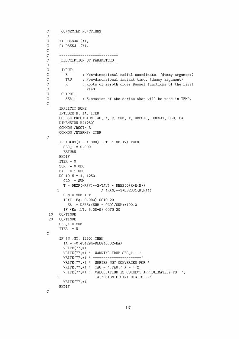
C CONNECTED FUNCTIONSC ---------------------C 1) DBESJ0 (X),C 2) DBESJ1 (X).CC ----------------------------C DESCRIPTION OF PARAMETERS:C ----------------------------C INPUT:C X : Non-dimensional radial coordinate. (dummy argument)C TAU : Non-dimensional instant time. (dummy argument)C R : Roots of zeroth order Bessel functions of the firstC kind.C OUTPUT:C SER_1 : Summation of the series that will be used in TEMP.C

IMPLICIT NONEINTEGER N, IA, ITERDOUBLE PRECISION TAU, X, R, SUM, T, DBESJ0, DBESJ1, OLD, EADIMENSION R(1250)COMMON /ROOT/ RCOMMON /NTERMS/ ITER

CIF (DABS(X - 1.0D0) .LT. 1.0D-12) THENSER_1 = 0.0D0RETURN

ENDIFITER = 0SUM = 0.0D0EA = 1.0D0DO 10 N = 1, 1250OLD = SUMT = DEXP(-R(N)**2*TAU) * DBESJ0(X*R(N))

1 / (R(N)**3*DBESJ1(R(N)))SUM = SUM + TIF(T .Eq. 0.0D0) GOTO 20EA = DABS((SUM - OLD)/SUM)*100.0

IF (EA .LT. 5.0D-9) GOTO 2010 CONTINUE20 CONTINUE

SER_1 = SUMITER = N

CIF (N .GT. 1250) THENIA = -0.434294*DLOG(0.02*EA)WRITE(77,*)WRITE(77,*) ’ WARNING FROM SER_1...’WRITE(77,*) ’ -----------------------’WRITE(77,*) ’ SERIES NOT CONVERGED FOR ’WRITE(77,*) ’ TAU = ’,TAU,’ X = ’,XWRITE(77,*) ’ CALCULATION IS CORRECT APPROXIMATELY TO ’,

1 IA,’ SIGNIFICANT DIGITS...’WRITE(77,*)

ENDIFC

131

RETURNEND

B.6 FUNCTION: SERIES 2

DOUBLE PRECISION FUNCTION SER_2 (TAU, X)C ----------C PURPOSE:C ----------C SER_2 is the summation of the series which is used in INT_1.C These series include Bessel roots (R) and one Bessel functionC (first order Bessel functions of the first kind). Initially, firstC 1250 roots of zeroth order Bessel functions of the first kind (R)C is found (it is possible to use any subroutine to find root ofC Bessel functions but it is not given here). Then first order BesselC functions of the first kind DBESJ1(R) are computed for each R (TheC algorithm of this Bessel function is not either given here).C Lastly, by substituting these Bessel function into the equation ofC T and adding for each R, SER_2 is calculated. All calculations areC done for non-dimensional parameters.CC ---------------------C CONNECTED FUNCTIONSC ---------------------C 1) DBESJ1 (X).CC ----------------------------C DESCRIPTION OF PARAMETERS:C ----------------------------C INPUT:C R : Roots of zeroth order Bessel functions of the firstC kind.C X : Non-dimensional radial coordinate. (dummy argument)C TAU : Non-dimensional instant time. (dummy argument)C OUTPUT:C SER_2 : Summation of the series that will be used in INT_1.C

IMPLICIT NONEINTEGER N, IA, ITERDOUBLE PRECISION TAU, X, R, SUM, T, DBESJ1, OLD, EADIMENSION R(1250)COMMON /ROOT/ RCOMMON /NTERMS/ ITER

CIF (X .Eq. 0.0D0) THENSER_2 = 0.0D0RETURN

ENDIFC

ITER = 0SUM = 0.0D0EA = 1.0D0DO 10 N = 1, 1250OLD = SUM

132

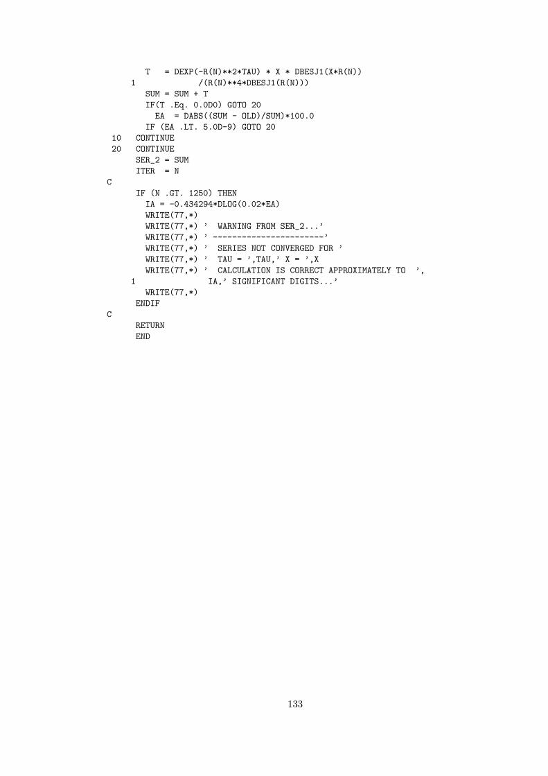
T = DEXP(-R(N)**2*TAU) * X * DBESJ1(X*R(N))1 /(R(N)**4*DBESJ1(R(N)))

SUM = SUM + TIF(T .Eq. 0.0D0) GOTO 20EA = DABS((SUM - OLD)/SUM)*100.0

IF (EA .LT. 5.0D-9) GOTO 2010 CONTINUE20 CONTINUE

SER_2 = SUMITER = N

CIF (N .GT. 1250) THENIA = -0.434294*DLOG(0.02*EA)WRITE(77,*)WRITE(77,*) ’ WARNING FROM SER_2...’WRITE(77,*) ’ -----------------------’WRITE(77,*) ’ SERIES NOT CONVERGED FOR ’WRITE(77,*) ’ TAU = ’,TAU,’ X = ’,XWRITE(77,*) ’ CALCULATION IS CORRECT APPROXIMATELY TO ’,

1 IA,’ SIGNIFICANT DIGITS...’WRITE(77,*)

ENDIFC

RETURNEND

133

APPENDIX C

FORTRAN CODES OF ELASTIC-PLASTIC STATE

C.1 MAIN PROGRAM: ELASTIC-PLASTIC STATE

PROGRAM ELASTIC PLASTIC STATEC ----------C PURPOSE:C ----------C This program is used to calculate the non-dimensional responseC variables in the elastic-plastic state for the problem of rotatingC solid shaft subjected to temperature cycle. All calculations areC done for non-dimensional parameters. In this state, six integrationC constants, 2 interface radius and the axial strain is need to beC computed. The integration constants are already calculatedC analytically in subroutine NLNEQN, which is externally called byC the present program, and they are moved to the current program byC COMMON command. However, resulting system of equations areC non-linear in the border radii. Hence, remaining three unknownsC are needed to be computed numerically. This is done by the PowellC Hybrid Method implemented in the program Minpack.for. Therefore,C HYBRD1 is called to solve three unknowns numerically. For theC present algorithm, input and output parameters are given below.C Furthermore, Subroutine ’DISTRIBUTION’ is used to calculate someC integrals which include temperature terms. By substituting variableC R, power M and the upper limits of the integral, INT1 and INT2E areC calculated analytically by this subroutine. Additionally, thisC subroutine is also used to get TBAR which is non-dimensionalC temperature distribution.C The problem is formulated for solid shaft. Hence, there is not anC inner radius. However, for numerical calculation, an inner surfaceC radius is needed to be defined. Therefore, a sufficiently smallC inner radius A is defined as 0.1D-10.C After the definition of input parameters (NU,Q,BETA,OMEGA,TAU,C TAUT,TAUC), initial estimates are done for EPS0, R1 and R2. TheseC estimations are sent to HYBRD1 with system of equations defined inC NLNEQN. If program converges perfectly with the tolerance defined,C input and output parameters are written into A-FIRST-STAGE.DAT.C Response variables are calculated for each regions at N1,N2 andC N3 points and results are printed to the same output file.CC -----------------------C CONNECTED SUBROUTINESC -----------------------

134

C 1) HYBRD1 (NLNEQN, ND, X, F, TOL, INFO, W, LW) (Implemented intoC Minpack.for),C 2) NLNEQN (NDIM, X, F, IFLAG) as External,C 3) PLAST1 (R, C3, C4, EPS0, U, SIGR, SIGT, SIGZ, EPSR, EPST,C EPSZ),C 4) PLAST2 (R, C5, C6, EPS0, U, SIGR, SIGT, SIGZ, EPSR, EPST,C EPSZ),C 5) ELAST (R, C1, C2, EPS0, U, SIGR, SIGT, SIGZ),C 6) DISTRIBUTION (R, TBAR, ULIM, INT1, POW, INT2E).CC ----------------------------C DESCRIPTION OF PARAMETERS:C ----------------------------C INPUT:C A : Sufficiently small inner radius for solid shaftC (it is assumed as 1.0D-10).C BETA : Non-dimensional temperature dependence parameter ofC the material.C C1-C6 : Non-dimensional integration constants (calculatedC analytically in subroutine NLNEQN and inserted toC the current program). (from COMMON block)C M : A power that is introduced in plastic region II.C ND : A positive integer input variable set to the numberC of functions and variables in non-linear equationC system solver.C NU : Poisson’s ratio.C N1,N2,N3: Number of data points in plastic region I, plasticC region II and elastic region, respectively.C OMEGA : Non-dimensional angular velocity.C Q : A non-dimensional measure for the maximum surfaceC temperature during the transient heating.C R : Non-dimensional radial coordinate.C TAU : Non-dimensional instant time.C TAUT : The non-dimensional time value when surface heatingC ends.C TAUC : The non-dimensional time value that the surfaceC temperature is held constant at maximum temperatureC value.C TOL : Tolerance on the solution of the nonlinear equationC system. It is a nonnegative input variable.C Termination occurs when the algorithm estimates thatC the relative error between X and this solution is atC most TOL.CC OUTPUT:C EPSR : Non-dimensional radial plastic strain.C EPST : Non-dimensional circumferential plastic strain.C EPSZ : Non-dimensional axial plastic strain.C EPS0 : Non-dimensional axial strain (initially estimated,C then exact value is computed).C INFO : An integer output variable which gives informationC concerning terminated execution in non-linear systemC solver.C R1 : Non-dimensional interface radius between plasticC region I and II (initially estimated, then exact

135

C value is computed).C R2 : Non-dimensional interface radius between plasticC region II and elastic region (initially estimated,C then exact value is computed).C SIGR : Non-dimensional radial stress component.C SIGT : Non-dimensional circumferential stress component.C SIGZ : Non-dimensional axial stress component.C SIGTHER : Non-dimensional yield stress.C SIGY : Non-dimensional equivalent stress.C U : Non-dimensional radial displacement component.C X : An array which the final estimate of the solutionC vector in HYBRD1).C

IMPLICIT NONEINTEGER I, N1, N2, N3, ND, LW, INFO, JPARAMETER ( ND = 3 )PARAMETER ( LW = ND * (3*ND + 13) )DOUBLE PRECISION R, DR, C1, C2, C3, C4, C5, C6, SIGR, SIGT,1 SIGZ, U, NU, OMEGA, F, M, A, TOL, R1, R2, EPSR,2 EPST, EPSZ, EPS0, Q, BETA, TAU, TAUT, TAUC,3 TBARINT1, TBARINT2, TBARINT3,TBARINT4, SIGY,X,4 TBARINTPM,TBARINTNM, XUP, XLO, TBARINT, TBAR, W,5 SIGTHER, INT2E, INT1, ULIM, POWDIMENSION X(ND), F(ND), W(LW)COMMON /PROP/ BETA, NU, Q, OMEGA, M, TAUT, TAUC, TAUCOMMON /CONS/ C1, C2, C3, C4, C5, C6EXTERNAL NLNEQN

COPEN (61,FILE=’A-FIRST-STAGE.DAT’)

CC --------------------------------------C Sufficiently small inner radius A for solid shaft is described.C

A = 0.1D-10M = DSQRT(1.0/(2.0*(1.0D0 - NU)))

CC -----------------------------------C MECHANICAL AND THERMAL PROPERTIESC -----------------------------------

NU = 0.3D0Q = 0.6D0BETA = 0.2D0

CC ------------------C ANGULAR VELOCITYC ------------------C The angular velocity is calculated as 90% of elastic limitC rotation speed for isothermal shaft.C

OMEGA = DSQRT(8.0*(1.0D0 - NU)/(3.0D0 - 4.0*NU))*0.9D0CC -----------------C TIME PARAMETERSC -----------------

TAU = 1.57d0

136

TAUT = 1.2D0TAUC = 0.3D0

CC -----------C TOLERANCEC -----------C Tolerance, which is used on the solution of the non-linearC equation system, is defined.C

TOL = 1.0D-10CC -------------------C INITIAL ESTIMATESC -------------------C Initial estimations for EPS0, R1 and R2 are presumed to beC used in non-linear equation system solver.C

EPS0 = 0.434827D0R1 = 0.100458D0R2 = 0.260047D0

C --------------------------------------C Argument X is described before it enters to the nonlinearC equation system solver.C

X(1) = EPS0X(2) = R1X(3) = R2

C --------------------------------------C Non-linear equation system solver (HYBRD1) is called. DuringC calling the solver, the subroutine NLNEQN is called as well.C

CALL HYBRD1 (NLNEQN, ND, X, F, TOL, INFO, W, LW)C --------------------------------------C The computed argument X in non-linear equation system solver isC equalized to the unknowns EPS0, R1 and R2.C

EPS0 = X(1)R1 = X(2)R2 = X(3)

C --------------------------------------C Convergence information of the results that are computed by theC non-linear equation system solver is screened.C

IF (INFO .Eq. 1) THENWRITE(6,*)WRITE(6,*) ’ -------------------------------------------------’WRITE(6,*) ’ FROM HYBRID: INFO = ’,INFOWRITE(6,*) ’ ITERATIONS CONVERGED PERFECTLY....’WRITE(6,*) ’ RESIDUALS ARE:’WRITE(6,*) ’ -------------------------------------------------’DO I = 1, NDWRITE(6,*) I, X(I), F(I)

END DOWRITE(6,*)

ELSE

137

WRITE(6,*) ’ FROM HYBRID: INFO = ’,INFOWRITE(6,*) ’ ITERATIONS DIVERGE !!!!’WRITE(6,*) ’ EXECUTION IS TERMINATED.’STOP

END IFC --------------------------------------C Input parameters and calculated unknowns are written to theC output file.C

WRITE(61,*) ’CONSTANTS ARE CALCULATED ANALYTICALLY’WRITE(61,*)WRITE(61,*) ’ MATERIAL PROPERTIES:’WRITE(61,*) ’ ------------------------------------------’WRITE(61,*) ’ NU = ’,NUWRITE(61,*) ’ Q = ’,QWRITE(61,*) ’ BETA = ’,BETAWRITE(61,*) ’ TEMPERATURE PROPERTIES:’WRITE(61,*) ’ ------------------------------------------’WRITE(61,*) ’ TAU = ’,TAUWRITE(61,*) ’ TAUT = ’,TAUTWRITE(61,*) ’ TAUC = ’,TAUC

CWRITE(61,*)WRITE(61,*) ’ LOAD PARAMETER (ANGULAR SPEED):’WRITE(61,*) ’ ------------------------------------------’WRITE(61,*) ’ OMEGA = ’,OMEGAWRITE(61,*)WRITE(61,*) ’ COMPUTING:’WRITE(61,*) ’ ------------------------------------------’WRITE(61,*) ’ TOLERANCE = ’,TOLWRITE(61,*)WRITE(61,*) ’ INTEGRATION CONSTANTS AND INT. RADIUS: ’WRITE(61,*) ’ ------------------------------------------’WRITE(61,*) ’ EPS0 = ’,EPS0WRITE(61,*) ’ R1 = ’,R1WRITE(61,*) ’ R2 = ’,R2WRITE(61,*) ’ C1 = ’,C1WRITE(61,*) ’ C2 = ’,C2WRITE(61,*) ’ C3 = ’,C3WRITE(61,*) ’ C4 = ’,C4WRITE(61,*) ’ C5 = ’,C5WRITE(61,*) ’ C6 = ’,C6

CWRITE(61,*)

CC --------------------------------------C Number of data points in plastic region I, plasticC region II and elastic region are defined.C

WRITE(6,*) ’ NUMBER OF DATA PTS. IN FIRST PLASTIC ?’READ(5,*) N1

WRITE(6,*) ’ NUMBER OF DATA PTS. IN SECOND PLASTIC ?’READ(5,*) N2

WRITE(6,*) ’ NUMBER OF DATA PTS. IN ELASTIC ?’READ(5,*) N3

138

CC --------------------------------------C Response variables at each region are calculated and writtenC to the output file. To operate this SUBROUTINE PLAST1,C SUBROUTINE PLAST2 and SUBROUTINE ELAST are called at eachC radial coordinate between interface radii. Additionally, toC calculate SIGTHER, it is need to be obtaining TBAR at differentC radial coordinate. Hence, subroutine DISTRIBUTION is called.C

DR = (R1-A) / (N1-1)R = AWRITE(61,99)WRITE(61,*)DO 10 I = 1, N1CALL PLAST1 (R, C3, C4, EPS0, U, SIGR, SIGT, SIGZ,

1 EPSR, EPST, EPSZ)SIGY = DMAX1(DABS(SIGR-SIGT),DABS(SIGR-SIGZ),

1 DABS(SIGT-SIGZ))CALL DISTRIBUTION (R, TBAR, ULIM, INT1, POW, INT2E)SIGTHER = (1 - BETA*TBAR)WRITE(61,100) R, SIGR, SIGT, SIGZ, U, SIGY/SIGTHER, EPSR, EPST,

1 EPSZR = R + DR

10 CONTINUEC

DR = (R2 - R1) / (N2 - 1)R = R1DO 20 I = 1, N2CALL PLAST2 (R, C5, C6, EPS0, U, SIGR, SIGT, SIGZ,

1 EPSR, EPST,EPSZ)SIGY = DMAX1(DABS(SIGR-SIGT),DABS(SIGR-SIGZ),

1 DABS(SIGT-SIGZ))CALL DISTRIBUTION (R, TBAR, ULIM, INT1, POW, INT2E)SIGTHER = (1 - BETA*TBAR)WRITE(61,100) R, SIGR, SIGT, SIGZ, U, SIGY/SIGTHER, EPSR, EPST,

1 EPSZR = R + DR

20 CONTINUEC

DR = (1-R2) / (N3-1)R = R2DO 30 I = 1, N3CALL ELAST (R, C1, C2, EPS0, U, SIGR, SIGT, SIGZ)SIGY = DMAX1(DABS(SIGR-SIGT),DABS(SIGR-SIGZ),

1 DABS(SIGT-SIGZ))CALL DISTRIBUTION (R, TBAR, ULIM, INT1, POW, INT2E)SIGTHER = (1 - BETA*TBAR)WRITE(61,100) R, SIGR, SIGT, SIGZ, U, SIGY/SIGTHERR = R + DR

30 CONTINUE

100 FORMAT(10(1X,F12.8))99 FORMAT(3X,’R’,12X,’SIGR’,9X,’SIGT’,9X,’SIGZ’,9X,’U’,12X,

1 ’SIGY/SIGTH’,3X,’EPSR’,9X,’EPST’,9X,’EPSZ’)C

139

END

C.2 SUBROUTINE: NLNEQN

SUBROUTINE NLNEQN (NDIM, X, F, IFLAG)C ----------C PURPOSE:C ----------C This subroutine is used to introduce functions F which describeC interface and boundary conditions. The array F is obtained andC sent to iterations in HYBRD1.C In each loop, estimated EPS0, R1 and R2 are taken from HYBRD1C and substituted into analytical expressions being for sixC integration constants. Then new F are computed by using interfaceC and boundary conditions and sent back to HYBRD1. These loops areC proceeding until the tolerance condition is satisfied in HYBRD1.C All expressions are in non-dimensional form.CC -----------------------C CONNECTED SUBROUTINESC -----------------------C 1) DISTRIBUTION (R, TBAR, ULIM, INT1, POW, INT2E).CC ----------------------------C DESCRIPTION OF PARAMETERS:C ----------------------------C INPUT:C EPS0 : Non-dimensional axial strain (exact value for EPS0C is taken from subroutine NLNEQN).C F : Functions, which include interface and boundaryC conditions, is used to estimate X.C R1 : Non-dimensional interface radius between plasticC region I and II (exact value for EPS0C is taken from subroutine NLNEQN).C R2 : Non-dimensional interface radius between plasticC region II and elastic region (exact value for EPS0C is taken from subroutine NLNEQN).C X : An array which the final estimate of the solutionC vector in HYBRD1) (dummy arguments)C OUTPUT:C C1-C6 : Non-dimensional integration constants (calculatedC analytically).C

IMPLICIT NONEINTEGER NDIM, IFLAG, ICALLDOUBLE PRECISION R, DR, C1, C2, C3, C4, C5, C6, SIGR, SIGT,1 SIGZ, U, NU, OMEGA, F, M, A, TOL, R1, R2, EPSR,2 EPST, EPSZ, EPS0, Q, BETA, TAU, TAUT, TAUC,3 T1, TBARINT, TBAR, SIGR1, SIGR2, SIGT1, SIGT2,4 U1, U2, SIGZ1, SIGZ2, EPSR2, EPST2,EPSZ2,5 EPSR1, EPST1, EPSZ1, U3, SIGR3, SIGT3, SIGZ3,6 T2,T3,T4,T5,T6,T7,K1,K2,K3, INT,X,XLO, XUP,7 TBARINTPM,TBARINTNM,TBARINT4,TBARINT3,TBARINT2,8 TBARINT1, TBARINT5, TBARINT6, POW,

140

9 INT2E, INT1, ULIMCOMMON /PROP/ BETA, NU, Q, OMEGA, M, TAUT, TAUC, TAUCOMMON /CONS/ C1, C2, C3, C4, C5, C6DIMENSION X(NDIM), F(NDIM)

CDATA ICALL / 0 /

CC --------------------------------------C Numerically estimated parameters EPS0, R1 and R2 in HYBRD1 areC written by using variable X.C

EPS0 = X(1)R1 = X(2)R2 = X(3)IFLAG = IFLAG

CC -----------------------C INTEGRATION CONSTANTSC -----------------------C Analytical expressions of the integration constants includesC EPS0, R1, R2, temperature terms and their integrals are written.C Different temperature integrals are called from subroutineC DISTRIBUTION to be inserted into the integration constants.CC

M = DSQRT(1.0/(2.0*(1.0D0 - NU)))POW = -MCALL DISTRIBUTION (R, TBAR, 1.0D0, INT1, POW, INT2E)TBARINT1 = INT1

CCALL DISTRIBUTION (R, TBAR, R2, INT1, POW, INT2E)TBARINT2 = INT1

CCALL DISTRIBUTION (R, TBAR, R1, INT1, POW, INT2E)TBARINT3 = INT2E

CCALL DISTRIBUTION (R, TBAR, R1, INT1, M, INT2E)TBARINT4 = INT2E

CCALL DISTRIBUTION (R, TBAR, R2, INT1, POW, INT2E)TBARINT5 = INT2E

CCALL DISTRIBUTION (R, TBAR, R2, INT1, M, INT2E)TBARINT6 = INT2E

CCALL DISTRIBUTION (R2, TBAR, ULIM, INT1, POW, INT2E)

CC1 = R2**2/(2.0*(1.0D0 + (1.0D0 - 2.0*NU)*R2**2))1 *((1.0D0 - 2.0*NU)*(R2**2 - 3.0D0 + 2.0*NU)*OMEGA**22 /(8.0D0*(1.0D0 - NU)) + 2.0*(1.0D0 + NU)*EPS0 + 1.0D03 - BETA*TBAR - 2.0*Q*(1.0D0 + NU)/(1.0D0 -NU)4 *((1.0D0 - 2.0*NU)*TBARINT1 + 1.0/(R2**2)*TBARINT2))

CC2 = (1.0D0 -2.0*NU)/(2.0*(1.0D0 + (1.0D0 - 2.0*NU)*R2**2))1 *(((1.0D0 - 2.0*NU)*R2**4 + 3.0D0 - 2.0*NU)*OMEGA**2

141

2 /(8.0*(1.0D0 - NU)) + 2.0*(R2**2 - NU/(1.0D0 - 2.0*NU))3 *EPS0 + R2**2*(1.0D0 - BETA*TBAR)4 + 2.0*Q*(1.0D0 + NU)/(1.0D0 - NU)*(TBARINT1 - TBARINT2))

CC4 = 0.0D0

CC5 = R2**(-M)/(2.0*M)*(-C1*(1.0D0 - M)/R2 + (1.0D0 + M)*R21 *(C2 - 1.0/2.0 - EPS0) - (3.0D0 + M)*(1.0D0 - 2.0*NU)**22 *OMEGA**2*R2**3/(16.0*(1.0D0 - NU)*(17.0D0 - 18.0*NU)))3 - Q*(1.0D0 - M)*(1.0D0 + NU)/(2.0*M*(1.0D0 - NU))4 *(R2**(-1.0D0 - M)*TBARINT2 - (1.0D0 + BETA5 *(1.0D0 - 2.0*NU)/(4.0*Q*(1.0D0 - M)*(1.0D0 + NU)))6 *TBARINT5)

CC6 = R2**M/(2.0*M)*(C1*(1.0D0 + M)/R2 - (1.0D0 - M)*R21 *(C2 - 1.0/2.0 - EPS0) + (3.0D0 - M)*(1.0D0 - 2.0*NU)**22 *OMEGA**2*R2**3/(16.0*(1.0D0 - NU)*(17.0D0 - 18.0*NU)))3 + Q*(1.0D0 + M)*(1.0D0 + NU)/(2.0*M*(1.0D0 - NU))4 *(R2**(-1.0D0 + M)*TBARINT2 - (1.0D0 + BETA5 *(1.0D0 - 2.0*NU)/(4.0*Q*(1.0D0 + M)*(1.0D0 + NU)))6 *TBARINT6)

CC3 = 2.0/(1.0D0 - 2.0*NU)*(C5*R1**(-1.0D0 + M)*(M*(1.0D0 - NU)1 + NU) - C6*R1**(-1.0D0 - M)*(M*(1.0D0 - NU)2 - NU) + (1.0D0 + NU)*EPS0 + 1.0/2.0) + 5.0*(1.0D0 - 2.0*NU)3 *OMEGA**2*R1**2/(2.0*(17.0D0 - 18.0*NU))4 - 1.0/(4.0*M*(1.0D0 - NU)*(1.0D0 - 2.0*NU))5 *(R1**(-1.0D0 + M)*(M*(1.0D0 - NU) + NU)6 *(4.0*Q*(1.0D0 - M)*(1.0D0 + NU) + BETA*(1.0D0 - 2.0*NU))7 *TBARINT3 + R1**(-1.0D0 - M)*(M*(1.0D0 - NU) - NU)8 *(4.0*Q*(1.0D0 + M)*(1.0D0 + NU) + BETA*(1.0D0 - 2.0*NU))9 *TBARINT4)

CC -----------------------------------------------------C AT R = R1 PLASTIC(1)-PLASTIC(2) INTERFACE CONDITIONC -----------------------------------------------------C At interface radius between plastic region I and plasticC region II (at R = R1), continuity of radial displacement isC satisfied with this condition. To generate F(1), subroutineC PLAST1 and PLAST2 are called, and difference of radial coordinateC is equalized to F(1).C

CALL PLAST1 (R1, C3, C4, EPS0, U1, SIGR1, SIGT1, SIGZ1,1 EPSR1, EPST1, EPSZ1)CALL PLAST2 (R1, C5, C6, EPS0, U2, SIGR2, SIGT2, SIGZ2,1 EPSR2, EPST2,EPSZ2)F(1) = U1 - U2

C -----------------------------------------------------C AT R = R1 PLASTIC(1)-PLASTIC(2) INTERFACE CONDITIONC -----------------------------------------------------C At interface radius R = R1, yielding condition for the plasticC region II should be satisfied. To generate F(2), subroutinesC PLAST2 and DISTRIBUTION are called.C

CALL PLAST2 (R1, C5, C6, EPS0, U1, SIGR1, SIGT1, SIGZ1,

142

1 EPSR1, EPST1,EPSZ1)CALL DISTRIBUTION (R1, TBAR, ULIM, INT1, POW, INT2E)F(2) = SIGR1 - SIGZ1 - 1.0D0 + BETA*TBAR

CC -----------------------------------C FORCE INTEGRAL BOUNDARY CONDITIONC -----------------------------------C This condition constitutes the total axial force on any sectionC that vanishes because of free ends of the shaft. For differentC temperature integrals, subroutine DISTRIBUTION is called and F(3)C is formed.C

CALL DISTRIBUTION (R, TBAR, 1.0D0, INT1, POW, INT2E)T1 = INT1

CALL DISTRIBUTION (R, TBAR, R2, INT1, POW, INT2E)T2 = INT1

CALL DISTRIBUTION (R, TBAR, R1, INT1, POW, INT2E)T3 = INT2E

CALL DISTRIBUTION (R, TBAR, R2, INT1, POW, INT2E)T4 = INT2E

CALL DISTRIBUTION (R, TBAR, R1, INT1, M, INT2E)T5 = INT2E

CALL DISTRIBUTION (R, TBAR, R2, INT1, M, INT2E)T6 = INT2E

CALL DISTRIBUTION (R, TBAR, R1, INT1, POW, INT2E)T7 = INT1

CK1 = (1.0D0 - 2.0*M*NU)*(4.0*Q*(1.0D0 + M)*(1.0D0 + NU)1 + BETA*(1.D0 - 2.0*NU))/(8.0*M*(1.0D0 - NU)2 *(1.0D0 - 2.0*NU))K2 = (1.0D0 + 2.0*M*NU)*(4.0*Q*(1.0D0 - M)*(1.0D0 + NU)1 + BETA*(1.D0 - 2.0*NU))/(8.0*M*(1.0D0 - NU)2 *(1.0D0 - 2.0*NU))K3 = -4.0*M*(1.0D0 - 2.0*NU)*(4.0*Q*(1.0D0 + NU)1 - BETA*(1.0D0 - NU))/(8.0*M*(1.0D0 - NU)2 *(1.0D0 - 2.0*NU))INT = -R1**2/2.0*(1.0D0 - C3)1 + 2.0*(1.0D0 - R2**2)*NU*C2/(1.0D0 - 2.0*NU)2 - (R1**(1.0D0 + M) - R2**(1.0D0 + M))*(1.0D0 + 2.0*M*NU)3 *C5/((1.0D0 + M)*(1.0D0 - 2.0*NU))4 - (R1**(1.0D0 - M) - R2**(1.0D0 - M))*(1.0D0 - 2.0*M*NU)5 *C6/((1.0D0 - M)*(1.0D0 - 2.0*NU))6 - NU*(R1**2 - R2**2)/(1.0D0 - 2.0*NU)7 + EPS0*(1.0D0 - NU*(1.0D0 - 2.0*R2**2)8 - R1**2*(1.0D0 + NU))/(1.0D0 - 2.0*NU)9 - OMEGA**2/8.0*(R1**4 - 2.0*(R1**4 - R2**4)1 *(1.0D0 + 6.0*NU)/(17.0D0 - 18.0*NU)2 + NU*(1.0D0 - R2**4)/(1.0D0 - NU))3 - 2.0*Q*(1.0D0 + NU)/(1.0D0 - NU)*T14 + (K3 - K1/(1.0D0 - M) + K2/(1.0D0 + M)5 + 2.0*Q*(1.0D0 + NU)/(1.0D0 - NU))*T26 + K2*R1**(1.0D0 + M)/(1.0D0 + M)*T37 - K2*R2**(1.0D0 + M)/(1.0D0 + M)*T48 - K1*R1**(1.0D0 - M)/(1.0D0 - M)*T59 + K1*R2**(1.0D0 - M)/(1.0D0 - M)*T6

143

1 + (BETA - K3 + K1/(1.0D0 - M) - K2/(1.0D0 + M))*T7F(3) = INT

CICALL = ICALL + 1WRITE(6,*) ’ *** NUMBER OF ITERATIONS = ’,ICALL

CRETURNEND

C.3 SUBROUTINE: PLASTIC REGION I

SUBROUTINE PLAST1 (R, C3, C4, EPS0, U, SIGR, SIGT, SIGZ,1 EPSR, EPST, EPSZ)

C ----------C PURPOSE:C ----------C Response variables in Plastic region I are computed at specifiedC radial coordinate R. The necessary input parameters are taken byC dummy arguments or by COMMON comment. All expressions are inC non-dimensional form.CC ------------------------C CONNECTED SUBROUTINES:C ------------------------C 1) DISTRIBUTION (R, TBAR, ULIM, INT1, POW, INT2E).CC ----------------------------C DESCRIPTION OF PARAMETERS:C ----------------------------C INPUT:C BETA : Non-dimensional temperature dependence parameter ofC the material.(from COMMON block)C C3, C4 : Two integration constants.(dummy arguments)C EPS0 : Non-dimensional axial strain. (dummy argument)C NU : Poisson’s ratio. (from COMMON block)C Q : A non-dimensional measure for the maximum surfaceC temperature during the transient heating. (from COMMONC block)C R : Non-dimensional radial coordinate. (dummy arguments)C TAU : Non-dimensional instant time. (from COMMON block)C TAUT : The non-dimensional time value when surface heatingC ends. (from COMMON block)C TAUC : The non-dimensional time value that the surfaceC temperature is held constant at maximum temperatureC value. (from COMMON block)CC OUTPUT:C EPSR : Non-dimensional radial plastic strain.C EPST : Non-dimensional circumferential plastic strain.C EPSZ : Non-dimensional axial plastic strain.C SIGR : Non-dimensional radial stress component.C SIGT : Non-dimensional circumferential stress component.C SIGZ : Non-dimensional axial stress component.C U : Non-dimensional radial displacement component.

144

CIMPLICIT NONEDOUBLE PRECISION R, C3, C4, EPS0, NU, OMEGA, BETA, TAU, TAUT,1 TAUC, U, SIGR, SIGT, SIGZ, EPSR, EPST,2 EPSZ, TBARINT, TBAR,Q, M, TEMP,3 INT1, POW, INT2E, ULIMCOMMON /PROP/ BETA, NU, Q, OMEGA, M, TAUT, TAUC, TAU

CC --------------------------------------C Subroutine ’DISTRIBUTION’ is called to obtain INT1. Upper limitC of the integral is R.C

CALL DISTRIBUTION (R, TBAR, R, INT1, POW, INT2E)TBARINT = INT1

CC --------------------------------------C Non-dimensional response variables are calculated.C

U = C4/R - EPS0*R/2.0 + 1.0/(4.0*(1.0D0 + NU)*R)1 *((1.0D0 - 2.0*NU)*R**2/4.0*(12.0*C3 - 4.0D0 - 3.02 *OMEGA**2*R**2) + 2.0*(6.0*Q*(1.0D0 + NU)3 + BETA*(1.0D0 - 2.0*NU))*TBARINT)

CSIGR = C3 - OMEGA**2*R**2/2.0

CSIGT = SIGR

CSIGZ = C3 - OMEGA**2*R**2/2.0 - (1.0D0 - BETA*TBAR)

CEPSR = -C4/R**2 - EPS0/2.0 + 1.0/(16.0*(1.0D0 + NU))1 *((1.0D0 - 2.0*NU)*(4.0*C3 - 5.0*OMEGA**2*R**2) - 4.0D02 - 8.0*(6.0*Q*(1.0D0 + NU) + BETA*(1.0D0 - 2.0*NU))/R**23 *TBARINT + 8.0*(4.0*Q*(1.0D0 + NU) + BETA*(1.0D0 - NU))4 *TBAR)

CEPST = C4/R**2 - EPS0/2.0 + 1.0/(16.0*(1.0D0 + NU))1 *((1.0D0 - 2.0*NU)*(4.0*C3 + OMEGA**2*R**2) - 4.0D02 + 8.0*(6.0*Q*(1.0D0 + NU) + BETA*(1.0D0 - 2.0*NU))/R**23 *TBARINT - 8.0*(2.0*Q*(1.0D0 + NU) - BETA*NU)*TBAR)

CEPSZ = -(EPSR + EPST)

CRETURNEND

C.4 SUBROUTINE: PLASTIC REGION II

SUBROUTINE PLAST2 (R, C5, C6, EPS0, U, SIGR, SIGT, SIGZ,1 EPSR, EPST,EPSZ)

C ----------C PURPOSE:C ----------C Response variables in Plastic region II are calculated at theC specified radial coordinates R. The necessary input parameters are

145

C taken by dummy arguments or by COMMON comment. All expressions areC in non-dimensional form.CC ------------------------C CONNECTED SUBROUTINES:C ------------------------C 1) DISTRIBUTION (R, TBAR, ULIM, INT1, POW, INT2E).CC ----------------------------C DESCRIPTION OF PARAMETERS:C ----------------------------C INPUT:C BETA : Non-dimensional temperature dependence parameter ofC the material. (from COMMON block)C C5, C6 : Two integration constants. (dummy arguments)C EPS0 : Non-dimensional axial strain. (dummy argument)C M : A power that is introduced in plastic region II. (fromC COMMON block)C NU : Poisson’s ratio. (from COMMON block)C Q : A non-dimensional measure for the maximum surfaceC temperature during the transient heating. (from COMMONC block)C R : Non-dimensional radial coordinate. (dummy argument)C TAU : Non-dimensional instant time. (from COMMON block)C TAUT : The non-dimensional time value when surface heatingC ends. (from COMMON block)C TAUC : The non-dimensional time value that the surfaceC temperature is held constant at maximum temperatureC value. (from COMMON block)CC OUTPUT:C EPSR : Non-dimensional radial plastic strain.C EPST : Non-dimensional circumferential plastic strain.C EPSZ : Non-dimensional axial plastic strain.C SIGR : Non-dimensional radial stress component.C SIGT : Non-dimensional circumferential stress component.C SIGZ : Non-dimensional axial stress component.C U : Non-dimensional radial displacement component.C

IMPLICIT NONEDOUBLE PRECISION R, C5, C6, EPS0, NU, OMEGA, BETA, TAU, TAUT,1 TAUC, U, SIGR, SIGT, SIGZ, EPSR, EPST,EPSZ,2 M, TBARINTPM, TBARINTNM, TBAR, Q, XUP, XLO, TBARINT,3 POW, TEMP, INT1, INT2ECOMMON /PROP/ BETA, NU, Q, OMEGA, M, TAUT, TAUC, TAU

CC --------------------------------------C Subroutine ’DISTRIBUTION’ is called to obtain INT2E withC different powers (M and -M). Upper limits of the integralsC are R.C

POW = -MCALL DISTRIBUTION (R, TBAR, R, INT1, M, INT2E)TBARINTPM = INT2ECALL DISTRIBUTION (R, TBAR, R, INT1, POW, INT2E)

146

TBARINTNM = INT2ECC --------------------------------------C Non-dimensional response variables are calculated.C

U = C5*R**M + C6/R**M + R*(EPS0 + 1.0/2.0)1 - (1.0D0 - 2.0*NU)*OMEGA**2*R**3/(17.0D0 - 18.0*NU)2 + 1.0/(8.0*M*(1.0D0 - NU))*((4.0*Q*(1.0D0 + M)3 *(1.0D0 + NU) + BETA*(1.0D0 - 2.0*NU))/R**M*TBARINTPM4 -R**M*(4.0*Q*(1.0D0 - M)*(1.0D0 + NU)5 + BETA*(1.0D0 - 2.0*NU))*TBARINTNM)

CSIGR = 2.0/(1.0D0 - 2.0*NU)*(C5*(M*(1.0D0 - NU) + NU)1 *R**(-1.0D0 + M) - C6*(M*(1.0D0 - NU) - NU)2 *R**(-1.0D0 - M) + (1.0D0 + NU)*EPS0 + 1.0/2.0)3 - 2.0*(3.0D0 - 2.0*NU)*OMEGA**2*R**2/(17.0D0 - 18.0*NU)4 - 1.0/(4.0*M*(1.0D0 - NU)*(1.0D0 - 2.0*NU))5 *((M*(1.0D0 - NU) + NU)*(4.0*Q*(1.0D0 - M)*(1.0D0 + NU)6 + BETA*(1.0D0 - 2.0*NU))*R**(-1.0D0 + M)*TBARINTNM7 +(M*(1.0D0 - NU) - NU)*(4.0*Q*(1.0D0 + M)*(1.0D0 + NU)8 + BETA*(1.0D0 - 2.0*NU))/(R**(1.0D0 + M))*TBARINTPM)

CSIGT = 1.0/(1.0D0 - 2.0*NU)*(C5*(1.0D0 + 2.0*M*NU)1 *R**(-1.0D0 + M) + C6*(1.0D0 - 2.0*M*NU)2 *R**(-1.0D0 - M) + 2.0*(1.0D0 + NU)*EPS0 + 1.0D0)3 - (1.0D0 + 6.0*NU)*OMEGA**2*R**2/(17.0D0 - 18.0*NU)4 - 1.0/(8.0*M*(1.0D0 - NU)*(1.0D0 - 2.0*NU))5 *((1.0D0 + 2.0*M*NU)*(4.0*Q*(1.0D0 - M)*(1.0D0 + NU)6 + BETA*(1.0D0 - 2.0*NU))*R**(-1.0D0 + M)*TBARINTNM7 - (1.0D0 - 2.0*M*NU)*(4.0*Q*(1.0D0 + M)*(1.0D0 + NU)8 + BETA*(1.0D0 - 2.0*NU))/(R**(1.0D0 + M))*TBARINTPM)9 - (4.0*Q*(1.0D0 + NU) + BETA*(1.0D0 - NU))1 /(2.0*(1.0D0 - NU))*TBAR

CSIGZ = SIGT - (1.0D0 - BETA*TBAR)

CEPSR = 0.0D0

CEPSZ = -1.0/2.0*(C5*R**(-1.0D0 + M) + C6/(R**(1.0D0 + M)))1 + (1.0D0 - 2.0*NU)*OMEGA**2*R**2/(2.0*(17.0D0 - 18.0*NU))2 + 1.0/(16.0*M*(1.0D0 - NU))*((4.0*Q*(1.0D0 - M)3 *(1.0D0 + NU) + BETA*(1.0D0 - 2.0*NU))*R**(-1.0D0 + M)4 *TBARINTNM - (4.0*Q*(1.0D0 + M)*(1.0D0 + NU)5 + BETA*(1.0D0 - 2.0*NU))/(R**(1.0D0 + M))*TBARINTPM)6 -BETA/4.0*TBAR

CEPST = -EPSZ

CRETURNEND

C.5 SUBROUTINE: ELASTIC REGION

SUBROUTINE ELAST (R, C1, C2, EPS0, U, SIGR, SIGT, SIGZ)

147

C ----------C PURPOSE:C ----------C Response variables in Elastic region are calculated at specifiedC radial coordinate R. The necessary input parameters are taken byC dummy arguments or by COMMON comment. All expressions are inC non-dimensional form.CC ------------------------C CONNECTED SUBROUTINES:C ------------------------C 1) DISTRIBUTION (R, TBAR, ULIM, INT1, POW, INT2E).CC ----------------------------C DESCRIPTION OF PARAMETERS:C ----------------------------C INPUT:C BETA : Non-dimensional temperature dependence parameter ofC the material. (from COMMON block)C C1, C2 : Two integration constants. (dummy arguments)C EPS0 : Non-dimensional axial strain. (dummy argument)C NU : Poisson’s ratio. (from COMMON block)C Q : A non-dimensional measure for the maximum surfaceC temperature during the transient heating. (from COMMONC block)C R : Non-dimensional radial coordinate. (dummy argument)C TAU : Non-dimensional instant time. (from COMMON block)C TAUT : The non-dimensional time value when surface heatingC ends. (from COMMON block)C TAUC : The non-dimensional time value that the surfaceC temperature is held constant at maximum temperatureC value. (from COMMON block)CC OUTPUT:C SIGR : Non-dimensional radial stress component.C SIGT : Non-dimensional circumferential stress component.C SIGZ : Non-dimensional axial stress component.C U : Non-dimensional radial displacement component.C

IMPLICIT NONEDOUBLE PRECISION R, C1, C2, EPS0, NU, OMEGA, BETA, TAU, TAUT,1 TAUC, U, SIGR, SIGT, SIGZ, TBAR, TBARINT, Q, M, TEMP,2 INT1, INT2E, POWCOMMON /PROP/ BETA, NU, Q, OMEGA, M, TAUT, TAUC, TAU

CC --------------------------------------C Subroutine ’DISTRIBUTION’ is called to obtain INT1. Upper limitC of the integral is R.C

CALL DISTRIBUTION (R, TBAR, R, INT1, POW, INT2E)TBARINT = INT1

CC --------------------------------------C Non-dimensional response variables are calculated.C

148

SIGR = -2.0*C1/(R**2) + 2.0*C2/(1.0D0 - 2.0*NU)1 + 2.0*NU*EPS0/(1.0D0 - 2.0*NU) - 1.0/(8.0*(1.0D0 - NU))2 *((3.0D0 - 2.0*NU)*OMEGA**2*R**2 + 16.0*Q*(1.0D0 + NU)3 /R**2*TBARINT)

CSIGT = 2.0*C1/(R**2) + 2.0*C2/(1.0D0 - 2.0*NU)1 + 2.0*NU*EPS0/(1.0D0 - 2.0*NU) - 1.0/(8.0*(1.0D0 - NU))2 *((1.0D0 + 2.0*NU)*OMEGA**2*R**2 + 16.0*Q*(1.0D0 + NU)3 /R**2*(R**2*TBAR - TBARINT))

CSIGZ = 4.0*C2*NU/(1.0D0 - 2.0*NU) + 2.0*(1.0D0 - NU)*EPS01 /(1.0D0 - 2.0*NU) - 1.0/(2.0*(1.0D0 - NU))2 *(NU*OMEGA**2*R**2 + 4.0*Q*(1.0D0 + NU)*TBAR)

CU = C1/R + C2*R - (1.0D0 - 2.0*NU)*OMEGA**2*R**31 /(16.0*(1.0D0 - NU)) + Q*(1.0D0 + NU)/(R*(1.0D0 - NU))2 *TBARINT

CRETURNEND

C.6 FUNCTION: TEMPERATURE INTEGRAL 2

DOUBLE PRECISION FUNCTION INT_2E (TAUT, M, TAU, ULIM)C ----------C PURPOSE:C ----------C This function calculates the exact integrals given below.CC ULIM MC INT_2E = / TBAR(TAU,Y) * Y * DYC 0C ORC ULIM -MC INT_2E = / TBAR(TAU,Y) * Y * DYC 0CC The term titled SER is a summation of series and it is calledC from function SER_3 (M, TAU, X). This summation includes BesselC functions and roots. All calculations are done for non-dimensionalC parameters.CC ---------------------C CONNECTED FUNCTIONSC ---------------------C 1) SER_3 (M, TAU, X).CC ----------------------------C DESCRIPTION OF PARAMETERS:C ----------------------------C INPUT:C M : A power that is introduced in plastic region II.C (dummy argument)C TAU : Non-dimensional instant time. (dummy argument)

149

C TAUT : The non-dimensional time value when surface heatingC ends. (dummy argument)C ULIM : Non-dimensional radial coordinate or upper limit ofC the integral. (dummy argument)C OUTPUT:C INT_2E : Non-dimensional weighted integral that is used in theC plastic region II.C

IMPLICIT NONEDOUBLE PRECISION TAUT, M, TAU, X, ULIM, T1, T2, SER, SER_3

CC --------------------------------------C If upper limit of the integral is zero, result of integral willC be zero since its lower limit is zero.C

IF (ULIM .Eq. 0.0D0) THENINT_2E = 0.0D0RETURN

ENDIFCC --------------------------------------C Upper limit of the integral is set radial coordinate X. ThenC summation of the series is called from SER_3 (M, TAU, X). Finally,C INT_2E is calculated.C

X = ULIMSER = SER_3 (M, TAU, X)T1 = (12.0D0 + 4.0*M)*TAU + (1.0D0 + M)*X**2 - (3.0D0 + M)T2 = 4.0*(1.0D0 + M)*(3.0D0 + M)INT_2E = X**(1.0D0 + M) * T1 / (T2*TAUT)1 + 2.0/(TAUT*(1.0D0 + M)) * SER

CRETURNEND

C.7 FUNCTION: SERIES 3

DOUBLE PRECISION FUNCTION SER_3 (M, TAU, X)C ----------C PURPOSE:C ----------C SER_3 is the summation of the series which is used in INT_2E.C These series include Bessel roots (R) and one Bessel functionC (first order Bessel functions of the first kind). Initially, firstC 1250 roots of zeroth order Bessel functions of the first kind (R)C is found (it is possible to use any subroutine to find root ofC Bessel functions but it is not given here). Then first order BesselC functions of the first kind DBESJ1(R) are computed for each R (TheC algorithm of this Bessel function is not either given here).C Furthermore, HYPPFQ(A1, A2, A3, Z) being a hypergeometric functionC is called. Finally, SER_3 is calculated by substituting BesselC functions for each root R and hypergeometric function into T. AllC calculations are done for non-dimensional parameters.C

150

C ---------------------C CONNECTED FUNCTIONSC ---------------------C 1) HYPPFQ (A ,B, C, X),C 2) DBESJ1 (X).CC ----------------------------C DESCRIPTION OF PARAMETERS:C ----------------------------C INPUT:C M : A power that is introduced in plastic region II.C (dummy argument)C R : Roots of zeroth order Bessel functions of the firstC kind.C X : Non-dimensional radial coordinate. (dummy argument)C TAU : Non-dimensional instant time. (dummy argument)C OUTPUT:C SER_3 : Summation of the series that will be used in INT_2E.C

IMPLICIT NONEINTEGER N, IA, ITERDOUBLE PRECISION TAU, X, R, SUM, T, DBESJ1, OLD, EA, A1, A2, A3,1 Z, M, HYPPFQDIMENSION R(1250)COMMON /ROOT/ RCOMMON /NTERMS/ ITER

CIF (X .Eq. 0.0D0) THENSER_3 = 0.0D0RETURN

ENDIFC

ITER = 0SUM = 0.0D0EA = 1.0D0A1 = 0.5D0 + M/2.0A2 = 1.0D0A3 = 1.5D0 + M/2.0DO 10 N = 1, 1250Z = - X**2 * R(N)**2/4.0OLD = SUMT = DEXP(-R(N)**2*TAU) * X**(1.0D0 + M)

1 * HYPPFQ(A1, A2, A3, Z) / (R(N)**3*DBESJ1(R(N)))SUM = SUM + TIF(T .Eq. 0.0D0) GOTO 20EA = DABS((SUM - OLD)/SUM)*100.0

IF (EA .LT. 5.0D-9) GOTO 2010 CONTINUE20 CONTINUE

SER_3 = SUMITER = N

CIF (N .GT. 1250) THENIA = -0.434294*DLOG(0.02*EA)WRITE(77,*)

151

WRITE(77,*) ’ WARNING FROM SER_3...’WRITE(77,*) ’ -----------------------’WRITE(77,*) ’ SERIES NOT CONVERGED FOR ’WRITE(77,*) ’ TAU = ’,TAU,’ X = ’,XWRITE(77,*) ’ CALCULATION IS CORRECT APPROXIMATELY TO ’,

1 IA,’ SIGNIFICANT DIGITS...’WRITE(77,*)

ENDIFC

RETURNEND

C.8 FUNCTION: HYPERGEOMETRIC FUNCTION

DOUBLE PRECISION FUNCTION HYPPFQ (A ,B, C, X)C ----------C PURPOSE:C ----------C This function calculates 1000 terms of the series ofC hypergeometric function. The arguments A, B and C are described andC the function generates each terms for each radial coordinate X.C Although the last terms of the series of the hypergeometricC function are very long and complicated, solution is converged veryC fast.CC ----------------------------C DESCRIPTION OF PARAMETERS:C ----------------------------C INPUT:C A, B, C : Arguments of the hypergeometric function. (dummyC arguments)C X : Non-dimensional radial coordinate. (dummy argument)C OUTPUT:C HYPPFQ : Series of hypergeometric functionC

IMPLICIT NONEINTEGER I, J, LASTDOUBLE PRECISION A, B, C, X, RELER, SUM, T, T1, T2, T3

CC... SPECIAL CASE:C

IF (A .Eq. 0.0D0 .OR. X .Eq. 0.0D0) THENHYPPFQ = 1.0D0RETURN

END IFC

RELER = 1.0D-12SUM = 1.0D0LAST = 1000

CDO 10 I = 1, LAST

CT1 = 1.0D0DO J = 0, I-1

152

T1 = T1 * (A + 1.0D0*J) / (J+1)END DO

CT2 = 1.0D0DO J = 0, I-1T2 = T2 * (B + 1.0D0*J)

END DOC

T3 = 1.0D0DO J = 0, I-1T3 = T3 * (C + 1.0D0*J)

END DOC

T = X**I * T1 / (T2 * T3)SUM = SUM + TIF (DABS(T) .LT. RELER) GOTO 20

C10 CONTINUE20 CONTINUE

HYPPFQ = SUMIF (I .GT. LAST)1 WRITE(*,*) ’ FROM HYPPFQ: SERIES DOES NOT CONVERGE...’

CRETURNEND

153

APPENDIX D

FORTRAN CODES OF UNLOADED STATE

D.1 MAIN PROGRAM: UNLOADED STATE

PROGRAM UNLOADED STATEC ----------C PURPOSE:C ----------C This program is used to calculate the non-dimensional responseC variables in the unloaded state for the problem of rotating solidC shaft subjected to temperature cycle. The input parameters radialC coordinate and permanent plastic strains are read from an inputC file ’A-PERSTRAIN.DAT’. This file includes radial coordinate andC permanent plastic strains at NTOT data points. Permanent plasticC strains at NTOT data point are the plastic strains which areC computed in the program ELASTIC PLASTIC STATE at time when theC unloading state starts. After reading these parameters from theC input file unknown constants C1, C2 and EPS0 are calculatedC analytically. During this calculation, subroutines ’DAVINT’ andC ’DISTRIBUTION’ are called.C Subroutine ’DAVINT’ is used to compute some integral numericallyC which include permanent plastic strains. During calling DAVINT,C argument X, integral function F, lower and upper limits of theC integrals are prescribed. Numerical result of the integral is ANS.C Subroutine ’DISTRIBUTION’ is used to calculate some integralsC which include temperature terms. By substituting variable X andC the upper limits of the integral, INT1 is calculated analyticallyC by this subroutine. Additionally, this subroutine is also usedC to get TBAR which is non-dimensional temperature distribution.C Then response variables are calculated by using subroutinesC above and analytical expressions at NTOT radial coordinates.C Results are written into the file ’A-OUTPUT.DAT’.C All calculations are done for non-dimensional parameters.CC --------------------------------------C CONNECTED SUBROUTINES AND DATA FILESC --------------------------------------C 1) A-PERSTRAIN.DAT,C 2) DAVINT (X, Y, N, XLO, XUP, ANS, IERR) (Implemented inC Davint.for),C 3) DISTRIBUTION (R, TBAR, ULIM, INT1, POW, INT2E).CC ----------------------------

154

C DESCRIPTION OF PARAMETERS:C ----------------------------C INPUT:C BETA : Non-dimensional temperature dependence parameter ofC the material.C EPSRP : An array which includes permanent plastic radialC strain at NTOT data points. These strains areC generated by using program ’ELASTIC PLASTIC STATE’C at the time value when unloading starts and writtenC into ’A-PERSTRAIN.DAT’. (from data file)C EPSTP : An array which includes permanent plastic circumferentialC strain at NTOT data points. These strains areC generated by using program ’ELASTIC PLASTIC STATE’C at the time value when unloading starts and writtenC into ’A-PERSTRAIN.DAT’. (from data file)C EPSZP : An array which includes permanent plastic axialC strain at NTOT data points. These strains areC generated by using program ’ELASTIC PLASTIC STATE’C at the time value when unloading starts and writtenC into ’A-PERSTRAIN.DAT’. (from data file)C NTOT : Number of data points. (according to data file)C NU : Poisson’s ratio.C OMEGA : Non-dimensional angular velocity.C Q : A non-dimensional measure for the maximum surfaceC temperature during the transient heating.C R : Non-dimensional radial coordinate.C TAU : Non-dimensional instant time.C TAUT : The non-dimensional time value when surface heatingC ends.C TAUC : The non-dimensional time value that the surfaceC temperature is held constant at maximum temperatureC value.C X : An array which include NTOT non-dimensional radialC coordinate values (R) and read from ’A-PERSTRAIN.DAT’.C X(1)=0 and X(NTOT)=1. (from data file)C OUTPUT:C C2 : Non-zero, non-dimensional integration constantC EPS0 : Non-dimensional axial strain.C EPSRPU : Non-dimensional permanent plastic radial strain whichC remains in the shaft during plastic flow.C EPSTPU : Non-dimensional permanent plastic circumferential strainC which remains in the shaft during plastic flow.C EPSZPU : Non-dimensional permanent plastic axial strain whichC remains in the shaft during plastic flow.C SIGR : Non-dimensional radial stress component.C SIGT : Non-dimensional circumferential stress component.C SIGZ : Non-dimensional axial stress component.C SIGTHER : Non-dimensional yield stress.C SIGY : Non-dimensional equivalent stress.C U : Non-dimensional radial displacement component.C

IMPLICIT NONEINTEGER I, NTOT, IERPARAMETER ( NTOT = 298 )DOUBLE PRECISION NU, Q, BETA, OMEGA, TAU, TAUT, TAUC, M,

155

1 X, EPSRP, EPSTP, C1, C2, EPS0, F, ANS,2 INTEPS1, INTEPS2,TBARINT, R, TBAR, INT1,3 POW, INT2E, TERM1, TERM2, TERM3, TERM4,4 SIGR, SIGT, SIGZ, SIGTHER, SIGY, U, EPSRPU,5 EPSTPU, EPSZP, EPSZPUDIMENSION X(NTOT), EPSRP(NTOT), EPSTP(NTOT), EPSZP(NTOT), F(NTOT)COMMON /PROP/ BETA, NU, Q, OMEGA, M, TAUT, TAUC, TAU

COPEN (51, FILE=’A-PERSTRAIN.DAT’)OPEN (61, FILE=’A-OUTPUT.DAT’)

CC --------------------------------------C M is described since it is used in COMMON blocks althoughC it is not used in unloaded state.C

M = DSQRT(1.0/(2.0*(1.0D0 - NU)))C -----------------------------------C MECHANICAL AND THERMAL PROPERTIESC -----------------------------------

NU = 0.3D0Q = 0.6D0BETA = 0.2D0

CC ------------------C ANGULAR VELOCITYC ------------------C The angular velocity is calculated as 90% of elastic limitC rotation speed for isothermal shaft.C

OMEGA = DSQRT(8.0*(1.0D0 - NU)/(3.0D0 - 4.0*NU))*0.9D0CC -----------------C TIME PARAMETERSC -----------------

TAU = 10.0D0TAUT = 1.2D0TAUC = 0.3D0

CC ---------------------------------------C Permanent plastic strains at NTOT radial coordinate are readC from input file ’A-PERSTRAIN.DAT’.C

DO I=1,NTOTREAD(51,*) X(I),EPSRP(I), EPSTP(I), EPSZP(I)

END DOCC -----------C CONSTANTSC -----------C The unknown constants C1, C2 and EPS0 are calculatedC analytically. Subroutine ’DAVINT’ is called to obtainC INTEPS1 and INTEPS2. Subroutine ’DISTRIBUTION’ is calledC to obtain INT1.C

C1 = 0.0D0

156

CF = (EPSRP - EPSTP)/XCALL DAVINT (X, F, NTOT, X(1), X(NTOT), ANS, IER)INTEPS1 = ANS

CF = X*(EPSRP + EPSTP)CALL DAVINT (X, F, NTOT, X(1), X(NTOT), ANS, IER)INTEPS2 = ANS

CCALL DISTRIBUTION (X(NTOT), TBAR, X(NTOT), INT1, POW, INT2E)TBARINT = INT1

CC2 = (3.0D0 - 5.0*NU)*OMEGA**2/(16.0*(1.0D0 - NU**2))1 - (1.0D0 - 2.0*NU)/(2.0*(1.0D0 - NU))*INTEPS12 + (INTEPS2/(2.0D0 - 2.0*NU))3 + Q*(1.0D0 - 3.0*NU)/(1.0D0 - NU)*TBARINT

CEPS0 = - NU*OMEGA**2/(4.0*(1.0D0 + NU))1 - 2.0*(INTEPS2) + 2.0*Q*TBARINT

CC --------------------------------------C Input parameters and calculated unknowns are written to theC output file ’A-OUTPUT.DAT’.C

WRITE(61,*)WRITE(61,*) ’UNLOADING STAGE’WRITE(61,*)WRITE(61,*) ’ DATA :’WRITE(61,*) ’ ------------------------------------------------’WRITE(61,*) ’ NU = ’,NUWRITE(61,*) ’ q = ’,QWRITE(61,*) ’ BETA = ’,BETAWRITE(61,*) ’ OMEGA = ’,OMEGAWRITE(61,*) ’ TAU = ’,TAUWRITE(61,*) ’ TAUT = ’,TAUTWRITE(61,*) ’ TAUC = ’,TAUCWRITE(61,*)WRITE(61,*) ’ CONSTANTS : ’WRITE(61,*) ’ --------------------------’WRITE(61,*) ’ C1 = ’,C1WRITE(61,*) ’ C2 = ’,C2WRITE(61,*) ’ EPS0 = ’,EPS0WRITE(61,*)

CWRITE(61,99)

CC --------------------------------------C A loop is generated to compute the response variables.C For the radial coordinates from R=0 to R=1, INTEPS1 and INTEPS2C are obtained by calling subroutine ’DAVINT’, TBARINT is computedC by using subroutine ’DISTRIBUTION’ in NTOT data points. LimitingC case for these integrals are described when R approaches to 0.C Lastly, the response variables are calculated at NTOT data pointsC and written into the output file.C

157

CDO I = 1, NTOTR = X(I)EPSRPU = EPSRP(I)EPSTPU = EPSTP(I)EPSZPU = EPSZP(I)

CF = (EPSRP - EPSTP)/XCALL DAVINT (X, F, NTOT, X(1), R, ANS, IER)INTEPS1 = ANS

CF = X*(EPSRP + EPSTP)CALL DAVINT (X, F, NTOT, X(1), R, ANS, IER)INTEPS2 = ANS

CCALL DISTRIBUTION (R, TBAR, R, INT1, POW, INT2E)TBARINT = INT1

CIF (R.EQ.X(1)) THENTERM2 = (EPSRP(1) + EPSTP(1))/2.0TERM1 = 0.0D0TERM3 = 0.0D0TERM4 = TBAR/2

ELSETERM2 = INTEPS2/R**2TERM1 = INTEPS2/RTERM3 = TBARINT/RTERM4 = 1.0/R**2*TBARINT

END IFC

SIGR = 2.0*C2/(1.0D0 - 2.0*NU)1 + 2.0*NU*EPS0/(1.0D0 - 2.0*NU) - 1.0/(8.0*(1.0D0 - NU))2 *((3.0D0 - 2.0*NU)*OMEGA**2*R**23 - 8.0*(INTEPS1 - (1.0D0 - 2.0*NU)*TERM2)4 + 16.0*Q*(1.0D0 + NU)*TERM4)

CSIGT = 2.0*C2/(1.0D0 - 2.0*NU)

1 + 2.0*NU*EPS0/(1.0D0 - 2.0*NU) - 1.0/(8.0*(1.0D0 - NU))2 *((1.0D0 + 2.0*NU)*OMEGA**2*R**23 + 8.0D0*(-2.0*NU*EPSRPU + 2.0*(1.0D0 - NU)*EPSTPU4 - INTEPS1 - (1.0D0 - 2.0*NU)*TERM2)5 + 16.0*Q*(1.0D0 + NU)*(TBAR - TERM4))

CSIGZ = 4.0*C2*NU/(1.0D0 - 2.0*NU) + 2.0*(1.0D0 - NU)*EPS0

1 /(1.0D0 - 2.0*NU) - 1.0/(2.0*(1.0D0 - NU))2 *(NU*OMEGA**2*R**2 + 4.0*Q*(1.0D0 + NU)*TBAR)3 + 2.0/(1.0D0 - NU)*(EPSRPU + (1.0D0 - NU)*EPSTPU4 + NU*INTEPS1)

CU = C2*R - (1.0D0 - 2.0*NU)*OMEGA**2*R**3

1 /(16.0*(1.0D0 - NU)) + (1.0D0 - 2.0*NU)2 /(2.0*(1.0D0 - NU))*(R*INTEPS1 + TERM1)3 + Q*(1.0D0 + NU)/(1.0D0 - NU)*TERM3

CSIGTHER = (1 - BETA*TBAR)

158

CSIGY = DMAX1(DABS(SIGR-SIGT),DABS(SIGR-SIGZ),

1 DABS(SIGT-SIGZ))WRITE(61,100) R, SIGR, SIGT, SIGZ, SIGY/SIGTHER, U, EPSRPU,

1 EPSTPU, EPSZPUEND DO

C100 FORMAT(10(1X,F12.8))99 FORMAT(3X,’R’,12X,’SIGR’,9X,’SIGT’,9X,’SIGZ’,8X,’SIGY/SIGTHER’,

1 2X,’U’,12X,’EPSR’,9X,’EPST’,9X,’EPSZ’)STOPEND

D.2 DATA FILE: PERMANENT PLASTIC STRAINS

Table D.1: Permanent plastic strains at τ ≥ 1.7882

R EPSRP EPSTP EPSZP R EPSRP EPSTP EPSZP1E-07 0.01894 0.01894 -0.0379 0.23584 0 0.02226 -0.0223

0.00235 0.01894 0.01894 -0.0379 0.23926 0 0.02209 -0.02210.0047 0.01893 0.01894 -0.0379 0.24268 0 0.02191 -0.0219

0.00704 0.01892 0.01894 -0.0379 0.24609 0 0.02174 -0.02170.00939 0.01891 0.01894 -0.0378 0.24951 0 0.02156 -0.02160.01174 0.01889 0.01895 -0.0378 0.25293 0 0.02138 -0.02140.01409 0.01887 0.01895 -0.0378 0.25634 0 0.0212 -0.02120.01643 0.01884 0.01895 -0.0378 0.25976 0 0.02102 -0.0210.01878 0.01881 0.01896 -0.0378 0.26318 0 0.02084 -0.02080.02113 0.01878 0.01897 -0.0377 0.26659 0 0.02066 -0.02070.02348 0.01874 0.01897 -0.0377 0.27001 0 0.02048 -0.02050.02583 0.0187 0.01898 -0.0377 0.27342 0 0.0203 -0.02030.02817 0.01866 0.01899 -0.0376 0.27684 0 0.02012 -0.02010.03052 0.01861 0.019 -0.0376 0.28026 0 0.01993 -0.01990.03287 0.01856 0.01901 -0.0376 0.28367 0 0.01975 -0.01970.03522 0.0185 0.01902 -0.0375 0.28709 0 0.01956 -0.01960.03756 0.01844 0.01903 -0.0375 0.29051 0 0.01938 -0.01940.03991 0.01838 0.01904 -0.0374 0.29392 0 0.01919 -0.01920.04226 0.01831 0.01905 -0.0374 0.29734 0 0.01901 -0.0190.04461 0.01824 0.01907 -0.0373 0.30076 0 0.01882 -0.01880.04696 0.01817 0.01908 -0.0372 0.30417 0 0.01863 -0.01860.0493 0.01809 0.01909 -0.0372 0.30759 0 0.01844 -0.0184

0.05165 0.01801 0.01911 -0.0371 0.311 0 0.01825 -0.01820.054 0.01792 0.01913 -0.037 0.31442 0 0.01805 -0.0181

0.05635 0.01783 0.01914 -0.037 0.31784 0 0.01786 -0.01790.05869 0.01773 0.01916 -0.0369 0.32125 0 0.01767 -0.0177

159

Table D.1 (cont’d)

R EPSRP EPSTP EPSZP R EPSRP EPSTP EPSZP0.06104 0.01764 0.01918 -0.0368 0.32467 0 0.01747 -0.01750.06339 0.01753 0.0192 -0.0367 0.32809 0 0.01728 -0.01730.06574 0.01743 0.01922 -0.0366 0.3315 0 0.01708 -0.01710.06809 0.01732 0.01924 -0.0366 0.33492 0 0.01688 -0.01690.07043 0.0172 0.01926 -0.0365 0.33834 0 0.01668 -0.01670.07278 0.01709 0.01928 -0.0364 0.34175 0 0.01648 -0.01650.07513 0.01697 0.0193 -0.0363 0.34517 0 0.01628 -0.01630.07748 0.01684 0.01932 -0.0362 0.34858 0 0.01607 -0.01610.07982 0.01671 0.01935 -0.0361 0.352 0 0.01587 -0.01590.08217 0.01658 0.01937 -0.036 0.35542 0 0.01567 -0.01570.08452 0.01644 0.0194 -0.0358 0.35883 0 0.01546 -0.01550.08687 0.0163 0.01942 -0.0357 0.36225 0 0.01525 -0.01530.08922 0.01616 0.01945 -0.0356 0.36567 0 0.01504 -0.0150.09156 0.01601 0.01948 -0.0355 0.36908 0 0.01483 -0.01480.09391 0.01586 0.01951 -0.0354 0.3725 0 0.01462 -0.01460.09626 0.0157 0.01954 -0.0352 0.37592 0 0.01441 -0.01440.09861 0.01554 0.01956 -0.0351 0.37933 0 0.01419 -0.01420.10095 0.01538 0.01959 -0.035 0.38275 0 0.01398 -0.0140.1033 0.01521 0.01963 -0.0348 0.38616 0 0.01376 -0.0138

0.10565 0.01504 0.01966 -0.0347 0.38958 0 0.01355 -0.01350.108 0.01486 0.01969 -0.0346 0.393 0 0.01333 -0.0133

0.11034 0.01468 0.01972 -0.0344 0.39641 0 0.01311 -0.01310.11269 0.0145 0.01976 -0.0343 0.39983 0 0.01289 -0.01290.11504 0.01431 0.01979 -0.0341 0.40325 0 0.01266 -0.01270.11739 0.01412 0.01983 -0.0339 0.40666 0 0.01244 -0.01240.11974 0.01393 0.01986 -0.0338 0.41008 0 0.01221 -0.01220.12208 0.01373 0.0199 -0.0336 0.41349 0 0.01199 -0.0120.12443 0.01352 0.01994 -0.0335 0.41691 0 0.01176 -0.01180.12678 0.01332 0.01998 -0.0333 0.42033 0 0.01153 -0.01150.12913 0.01311 0.02001 -0.0331 0.42374 0 0.0113 -0.01130.13147 0.01289 0.02005 -0.0329 0.42716 0 0.01107 -0.01110.13382 0.01268 0.02009 -0.0328 0.43058 0 0.01083 -0.01080.13617 0.01245 0.02014 -0.0326 0.43399 0 0.0106 -0.01060.13852 0.01223 0.02018 -0.0324 0.43741 0 0.01036 -0.01040.14087 0.012 0.02022 -0.0322 0.44083 0 0.01012 -0.01010.14321 0.01176 0.02026 -0.032 0.44424 0 0.00988 -0.00990.14556 0.01153 0.02031 -0.0318 0.44766 0 0.00964 -0.00960.14791 0.01129 0.02035 -0.0316 0.45107 0 0.0094 -0.00940.15026 0.01104 0.0204 -0.0314 0.45449 0 0.00916 -0.00920.1526 0.01079 0.02044 -0.0312 0.45791 0 0.00891 -0.0089

0.15495 0.01054 0.02049 -0.031 0.46132 0 0.00867 -0.00870.1573 0.01028 0.02054 -0.0308 0.46474 0 0.00842 -0.0084

0.15965 0.01002 0.02059 -0.0306 0.46816 0 0.00817 -0.00820.162 0.00976 0.02063 -0.0304 0.47157 0 0.00792 -0.0079

0.16434 0.00949 0.02068 -0.0302 0.47499 0 0.00767 -0.00770.16669 0.00922 0.02073 -0.0299 0.47841 0 0.00741 -0.0074

160

Table D.1 (cont’d)

R EPSRP EPSTP EPSZP R EPSRP EPSTP EPSZP0.16904 0.00894 0.02079 -0.0297 0.48182 0 0.00716 -0.00720.17139 0.00866 0.02084 -0.0295 0.48524 0 0.0069 -0.00690.17373 0.00837 0.02089 -0.0293 0.48865 0 0.00664 -0.00660.17608 0.00809 0.02094 -0.029 0.49207 0 0.00639 -0.00640.17843 0.00779 0.021 -0.0288 0.49549 0 0.00612 -0.00610.18078 0.0075 0.02105 -0.0286 0.4989 0 0.00586 -0.00590.18313 0.0072 0.02111 -0.0283 0.50232 0 0.0056 -0.00560.18547 0.0069 0.02116 -0.0281 0.50574 0 0.00533 -0.00530.18782 0.00659 0.02122 -0.0278 0.50915 0 0.00507 -0.00510.19017 0.00628 0.02128 -0.0276 0.51257 0 0.0048 -0.00480.19252 0.00596 0.02134 -0.0273 0.51599 0 0.00453 -0.00450.19486 0.00564 0.0214 -0.027 0.5194 0 0.00426 -0.00430.19721 0.00532 0.02146 -0.0268 0.52282 0 0.00398 -0.0040.19956 0.00499 0.02152 -0.0265 0.52623 0 0.00371 -0.00370.20191 0.00466 0.02158 -0.0262 0.52965 0 0.00343 -0.00340.20426 0.00433 0.02164 -0.026 0.53307 0 0.00316 -0.00320.2066 0.00399 0.0217 -0.0257 0.53648 0 0.00288 -0.0029

0.20895 0.00364 0.02177 -0.0254 0.5399 0 0.0026 -0.00260.2113 0.0033 0.02183 -0.0251 0.54332 0 0.00231 -0.0023

0.21365 0.00295 0.02189 -0.0248 0.54673 0 0.00203 -0.0020.21599 0.00259 0.02196 -0.0246 0.55015 0 0.00174 -0.00170.21834 0.00223 0.02203 -0.0243 0.55357 0 0.00146 -0.00150.22069 0.00187 0.02209 -0.024 0.55698 0 0.00117 -0.00120.22304 0.0015 0.02216 -0.0237 0.5604 0 0.00088 -0.00090.22539 0.00113 0.02223 -0.0234 0.56381 0 0.00059 -0.00060.22773 0.00076 0.0223 -0.0231 0.56723 0 0.00029 -0.00030.23008 0.00038 0.02237 -0.0228 0.57065 0 0 00.23243 0 0.02244 -0.0224 1 0 0 0

161

162

CURRICULUM VITAE

PERSONEL INFORMATION

Surname, Name : Arslan, Eray

Nationality : Turkish (TC)

Date and Place of Birth : 1 July 1981, Adana

Marital Status : Single

Email : erarslan@metu.edu.tr

EDUCATION

Degree Institution Year of Graduation BS Çukurova University Mechanical Eng. 2003 High School Halide Edip Lisesi, Ankara 1998 WORK EXPERIENCE

Year Place Enrollment 2004-Present METU Department of Engineering Sciences Research Assistant

FOREIGN LANGUAGES

Advanced English, Basic German PUBLICATIONS

1) Arslan E., Mack W., Eraslan, A.N.: The rotating elastic-plastic hollow shaft conveying

a hot medium. Forschung im Ingenieurwesen / Engineering Research. (to appear).

2) Arslan E., Eraslan, A.N.: Analytical solution to the bending of a nonlinearly hardening

wide curved bar. Acta Mechanica 210, 71-84 (2010).

3) Eraslan, A.N., Arslan E.: A Computational Study on the Nonlinear Hardening Curved

Beam Problem. International Journal of Pure and Applied Mathematics 43, 129-143

(2008).

4) Eraslan, A.N., Arslan E.: A Concise Analytical Treatment of Elastic-plastic Bending of

a Strain Hardening Curved Beam. Zeitschrift für Angewandte Mathematik und Mechanik

(ZAMM) 88 No. 8, 600-616 (2008).

5) Arslan E., Mack W., Eraslan, A.N.: Effect of a temperature cycle on a rotating elastic-

plastic shaft. Acta Mechanica 195, 129-140 (2008).

163

6) Eraslan, A.N., Arslan E.: Plane Strain Analytical Solutions to Rotating Partially Plastic

Graded Hollow Shafts. Turkish Journal of Engineering and Environmental Sciences 31,

273-288 (2007).

7) Eraslan, A.N., Arslan E., Mack W.: The strain hardening rotating hollow shaft subject

to positive temperature gradient. Acta Mechanica 194, 191-211 (2007).

INTERNATIONAL CONFERENCE PROCEEDINGS

1) Arslan, E., Mack, W., Eraslan, A. N., ''The rotating elastic-plastic hollow shaft heated

at its inner surface'', 80th Annual Meeting of the International Association of Applied

Mathematics and Mechanics (GAMM), Gdansk, Poland, 4-9 February 2009.

2) Arslan, E., Mack, W., Eraslan, A. N., ''Transient heating of a rotating elastic-plastic

solid shaft'', 79th Annual Meeting of the International Association of Applied

Mathematics and Mechanics (GAMM), Bremen, Germany, 31 March- 4 April 2008,

(PAMM · Proc. Appl. Math. Mech. 8, 10257 – 10258 (2008) / DOI 10.1002 /

pamm.200810257).

3) Arslan, E., Eraslan, A. N., Mack, W. ''Elastic–plastic states of a rotating

inhomogeneously heated strain hardening hollow shaft'', 6th International Congress on

Industrial and Applied Mathematics GA/CT1952/004, Zurich, Switzerland, 16-20 July

2007, (PAMM Proc. Appl. Math. Mech. 7, 4040051 – 4040052 (2007) / DOI 10.1002 /

pamm.200701082)

4) Eraslan, A. N., Arslan, E., ''Numerical Solution of Partially Plastic Curved Beam

Problem'', III European Conference on Computational Mechanics Solids, Structures and

Coupled Problems in Engineering, Lisbon, Portugal, 5-8 June 2006, proceeding no: 1232.

NATIONAL CONFERENCE PROCEEDINGS

1) Arslan E., Eraslan, A. N. ''Doğrusal Olmayan Pekleşme Davranışı Gösteren

Eğri Eksenli Kirişin Basit Eğilme Altında Analitik Çözümü: Kısmen Plastik ve

Artık Gerilme Halleri'', 16. Ulusal Mekanik Kongresi, Kayseri, Nisan 2009.

2) Arslan E., Eraslan, A. N. ''Kısmen Plastik Eğri Eksenli Kiriş Probleminin Basit

Eğilme için Analitik Çözümü'', 15. Ulusal Mekanik Kongresi, Isparta, Eylül 2007,

pp. 117-124.

3) Eraslan, A. N., Arslan E. ''Fonksiyonel Derecelendirilmiş Dönen Milin

Elastoplastik Analitik Çözümü'', 14. Ulusal Mekanik Kongresi, Antakya, Eylül

2005, pp. 389-395.