Efficient Selection of Disambiguating Actions for Stereo Vision

Monika Schaeffer and Ronald ParrDuke University

Department of Computer Science{monika,parr}@cs.duke.edu

Abstract

In many domains that involve the use of sensors,such as robotics or sensor networks, there are op-portunities to use some form of active sensing todisambiguate data from noisy or unreliable sen-sors. These disambiguating actions typically taketime and expend energy. One way to choose thenext disambiguating action is to select the actionwith the greatest expected entropy reduction, orinformation gain. In this work, we consider ac-tive sensing in aid of stereo vision for robotics.Stereo vision is a powerful sensing technique formobile robots, but it can fail in scenes that lackstrong texture. In such cases, a structured lightsource, such as vertical laser line, can be usedfor disambiguation. By treating the stereo match-ing problem as a specially structured HMM-likegraphical model, we demonstrate that for a scanline with n columns and maximum stereo dis-parity d, the entropy minimizing aim point forthe laser can be selected in O(nd) time - costno greater than the stereo algorithm itself. Atypical HMM formulation would suggest at leastO(nd2) time for the entropy calculation alone.

1 Introduction

In many domains that involve the use of sensors, such asrobotics or sensor networks, there are opportunities to usesome form of active sensing to disambiguate data fromnoisy or unreliable sensors. These disambiguating actionstypically take time and expend energy, so some care mustbe exercised to choose these actions wisely.

In the field of robotics, laser range finders have been thesensor of choice in recent years due to their great accu-racy. However, there are many disadvantages to laser rangefinders. Even the two-dimensional models are expensiveand bulky, with calibrated moving parts that consume a lot

of power. They are also far from stealthy, an importantconsideration for some applications. Three-dimensionallaser range finders share the shortcomings of their two-dimensional counterparts at ten to twenty times the cost.

Recent advances in camera technology have made camerasan inexpensive and versatile sensor for many applications.When used in a stereo pair, they have the potential to re-place laser range finders as accurate depth sensing devicessince recent advances in the pixel density of cameras can, inprinciple, permit more accurate depth estimates over largerdistances.

While standard stereo algorithms are known to performwell on some highly textured benchmark images [7], theyhave trouble in scenes with little texture, such as the longblank walls often encountered in indoor robotics applica-tions. One way to address this problem is to introducetexture into the scene through the use of a structured lightsource. If size, time, and stealth are not considerations,and the target is neither far away nor brightly illuminated,a sequence of computer generated patterns from a projec-tor can be used for disambiguation [8]. However, in manyapplications, such a blanket approach is not practical.

In this paper, we consider a more concentrated light source,specifically a laser line projector, mounted on a pan-tilthead. A laser line projector can cover an entire verticalstripe through a scene with fairly bright light, yet it is com-pact and inexpensive. Moving the laser and projecting alaser line for each of the thousands of columns in a highresolution image would be rather time consuming. Sinceinformation propagates horizontally though the stereo al-gorithm, precise control of the pan-tilt head is not needed –a laser aim improves accuracy in many of the pixels adja-cent to the area struck by the laser. In addition, we integratethe laser into a stereo vision algorithm for a cycle that firstestimates stereo disparity, then selects and optimal querypoint for the laser, then repeats – hopefully as few times asneeded to get good estimates of depth.

The problem of selecting the best information gathering ac-tion is, in general, a quite difficult form of metacomputa-

tion. A poor technique for deciding where to aim the lasercould easily spend more time deliberating than it wouldtake to sweep the laser through every column in the im-age. Here we consider the aim point for the laser with thegreatest expected entropy reduction, or information gain,in the space of stereo matchings. This is a myopic pro-cedure, but it does quite well in practice and, importantly,it can be computed very efficiently. By converting an ex-isting dynamic programming stereo vision approach to anequivalent, highly structured HMM problem, we can thenapply insights from HMM information gain computationsto the problem, allowing us to calculate the expected en-tropy reduction of each potential laser line very efficiently.We demonstrate that for a scan line with n columns andmaximum stereo disparity d, the entropy minimizing aimpoint for the laser can be selected in O(nd) time - cost nogreater than the stereo algorithm itself. In contrast, a typi-cal HMM formulation would suggest at least O(nd2) timefor the entropy calculation alone.

We present results of this approach on synthetic benchmarkproblems and on a set of images collected by a prototypedevice that implements these ideas.

2 Augmenting Stereo Vision with Lasers

A typical stereo algorithm assumes that its input images arecaptured by two capture media, e.g. solid state sensors, thatare in the same plane, have identical (ideal) lenses, and arealigned so that corresponding rows of pixels in each im-age are on the same line. Even if this assumption is notentirely true (as it rarely is), it is assumed that the imagesare rectified in software to approximate this ideal. Pixel-to-pixel stereo algorithms work by finding, for each pixelin one frame, a corresponding pixel in the other frame (ordeclaring the pixel to be occluded). The assumption of acalibrated camera system limits the scope of this searchto pixels along the corresponding scan line in the adjacentframe, thereby permitting relatively efficient stereo algo-rithms. When a correct match is found, the depth can re-covered straightforwardly from the difference in horizontaloffsets of the pixels (the disparity) and the geometry of thecamera system.

Bobick and Intille [3] present stereo vision as a shortestpath problem through a data structure called the disparityspace image (DSI), which, for a horizontal scanline acrossa stereo image pair, captures information about all poten-tial matches between left and right image pixels. (In theirsimplest form, stereo algorithms assume independence be-tween horizontal scan lines. Elaborations are, of course,both possible and frequent.) The DSI is an n × d matrixof cells, each of which may take one of three possible val-ues. There are no more than 7 transitions in and out of eachcell and no cycles. Edge costs between cells correspondto either a match quality score based upon the luminance

i: location of the pixel in the right imagej: disparity valueM : A matched pixelL: A left image occlusion with penalty Dl

R: A right image occlusion with penalty Dr

score(i, j): pixel value difference between images

from node to node cost(i,j,M) (i,j-1,L) Dl

(i,j,M) (i+1,j,M) score(i+1,j)(i,j,M) (i+1,j+1,R) Dr

(i,j,L) (i,j-1,R) Dl

(i,j,L) (i+1,j,M) score(i+1,j)(i,j,R) (i+1,j,M) score(i+1,j)(i,j,R) (i+1,j+1,R) Dr

Figure 1: Node transition costs when viewing the DSI as agraphical model.

of difference between the pixels that are matched, or oc-clusion penalty score for failing to match a pixel. Thus,the lowest cost path through the graph corresponds to thebest stereo matching. The main advantage of the DSI viewof the stereo problem is that the sparseness and regularityof the DSI structure permit a dynamic programming solu-tion to the shortest path problem in a single scan line inO(nd) time. This view also implicitly encodes two con-straints on the space of possible matchings, the uniquenessconstraint and the ordering constraint. The uniqueness con-straint permits each pixel to match at most one other pixel.The ordering constraint requires that the indices of matchesalong any row of the image are non-decreasing (increas-ing when combined with the uniqueness constraint). Theconsequences of these assumptions are discussed in moredetail in Section 2.4.

2.1 The Disparity Space Image

We view the DSI as a graphical model with n×d×3 nodesand the arc costs shown in Figure 1. The graphical struc-ture is shown in Figure 2. The path costs in the originalDSI induce a measure on the space of matchings. We there-fore convert the DSI costs to unnormalized potentials in agraphical model by exponentiating negated scores. (In thisview, a score that is a squared luminance difference corre-sponds to a Gaussian sensor noise model.) We can nowview the DSI as defining an HMM-like chain graphicalmodel where the individual states have internal structure.The set of nodes (i, ∗, ∗) collectively define the distributionover the disparity values of pixel i in the image and corre-spond to a single HMM state. The arcs between (i, ∗, ∗)and (i+1, ∗, ∗) define the (non-stationary) transition prob-abilities between adjacent states.

The benefit of this representation over a standard HMMformulation is that we can use a modified version of theforward-backward algorithm that exploits the internal state

Figure 2: A collection of nodes internal to the DSI, with theseven transitions out of a triplet of nodes highlighted. Thispattern repeats to the ends of the DSI. Within a column, Mand R nodes are jointly exhaustive and mutually exclusive.The L nodes encode a more complicated set of transitionsbetween Ms in adjacent columns, while keeping the entiregraph to a low degree.

structure. For each node in the DSI, we compute the incom-ing path costs in both the forward and backward directions.These can then be normalized (within M and R events) toproduce a distribution over events for each pixel in the rightimage. This is valid because the M and R nodes are mu-tually exclusive and jointly exhaustive events for a givenpixel in the right frame. While we have presented this al-gorithm from the perspective of the right camera, there isno loss of generality in doing so – values can be computedfor the left camera in a similar manner.

In Section 2.2, we will present dynamic programming al-gorithms that use the sparseness of the DSI to compute theViterbi path, marginal probability distributions, and pathentropy for this model in O(nd) time.

Creating the original DSI

To visualize the transition costs, Disparity Space Image canbe viewed literally as an image. The top of the image rep-resents high disparity values (objects that are closer to thecamera), and the bottom of the image represents low dis-parity values. The image represents the cost function overthe M nodes in the DSI. A pixel takes on the value of thetransition cost into the M node at that (column, disparity)pair.

Every row in the DSI corresponds to a different disparitylevel at which pixels in the left image can match pixels inthe right image. When the DSI is created from the per-spective of the right camera, a scan line in the right im-age is projected into disparity space by simply repeatingthe image scanline d times (Figure 3a). A left scan line isprojected into disparity space by sliding it horizontally as

(a) The right scanline in disparity space

(b) The left scanline in disparity space

(c) The DSI combines these

(d) Shortest Path overlayed

Figure 3: The DSI as an image: (a) The right scanline, (b)The left scanline, (c) The DSI, and (d) the shortest path.

the disparity level (vertical dimension in the DSI) changes(Figure 3b). The final DSI is then the difference betweenthe these right and left images, with a cost function applied(Figure 3c). These scores become unnormalized log prob-abilities of transition into the M nodes in the graph viewof the DSI. On an intuitive level, the most probable paththrough the DSI image is the light band (or dark, depend-ing on your choice of scaling) visible where matchings aregood (Figure 3d). This path is found by dynamic program-ming (Section 2.2).

Updating the DSI as laser results come in

At naturally occurring strong boundaries in the image pair(idealized as a two-tone vertically separated field in Fig-ure 4), the DSI takes on a slanted X-shaped pattern, withthe ideal matching corresponding to a path through the cruxof the X. If the boundary is strong enough, this dividesthe shortest path problem into two independent problems.When we get a matching from our laser aim, we would liketo get the same problem-splitting effect. We achieve this byfilling nodes with impossibly high transition costs with thesame X pattern, funneling all paths through the one match-ing point.

2.2 The DP Stereo Algorithm

Each node in the graph-DSI has at most three predecessornodes and three successor nodes. Because of the sparse na-ture of the graph, we can calculate the shortest path throughit in linear time using dynamic programming. With someslight modification to the dynamic programming algorithm,we can also calculate the marginal probability of any node

Figure 4: An X pattern in the DSI naturally generated atedges in the image. The effect is reproduced when the laseridentifies a match. All nodes internal to the two trianglesare blocked. Transitions to along the boundary are assignedvery low probability. The L nodes above the established Mnode and R nodes following the M down the diagonal areexceptions, as discussed in detail in section 2.4.

(a)node c Γ−(c)

(i,j,M) (i-1,j,M) (i-1,j,L) (i-1,j,R)(i,j,R) (i-1,j-1,M) (i-1,j-1,R)(i,j,L) (i,j+1,M) (i,j+1,L)

(b)node c Γ+(c)

(i,j,M) (i+1,j,M) (i,j-1,L) (i+1,j+1,R)(i,j,R) (i+1,j,M) (i+1,j+1,R)(i,j,L) (i+1,j,M) (i,j-1,L)

Figure 5: Each node has at most three predecessor nodes(a) and three successor nodes (b).

and the path entropy through any node in linear time. Thesemodifications require running the dynamic program bothforwards and backwards over the graph. In the forwarddirection, the algorithm moves in the direction of the arcsin the DSI and computes a value for each node as func-tion of its predecessor’s values. In the backward direction,the algorithm moves against the direction of the arcs in theDSI and computes a value for each node as a function thenode’s successor values. The predecessor and successorsets, Γ−(c) and Γ+(c), respectively, are defined in Fig-ure 2.2.

Dynamic Programming to find the shortest path

We begin by reconstructing the Bobick and Intille algo-rithm as a Viterbi path calculation through a graph. Tofind the best path, we iterate over the nodes in a columnfrom bottom to top, moving left to right through the DSI.For each node, we consider the legal transitions into thenode and select the lowest cost. We store this value as wellas backward pointer indicating which predecessor gives usthe value.

sp(c) = score(c) + minb∈Γ−(c)

sp(b)

At the end of the forward DP pass, we select the shortestpath for all exit nodes and, using the backwards pointers,reconstruct the path which provides this lowest cost. If weview scores as negated log probabilities, the path with min-imum score is equivalent to the path with highest probabil-ity, i.e., the Viterbi path.

Modification to find marginals and path entropy

The marginal probabilities over events in the DSI canbe computed by an adaptation of the standard forward-backward procedure for HMMs:

pf (c) = e−score(c) ∗∑

b∈Γ−(c)

pf (b)

pb(c) = e−score(c) ∗∑

b∈Γ+(c)

pb(b)

p(c) ∝ pf (c) ∗ pb(c)

After running DP backwards and forwards, we normalizethe probabilities over M and R for each pixel. To calculatethe entropy of all paths running through a node we run thedynamic program:

hf (c) = pf (c)∑

b∈Γ−(c)

(pf (b) log(pf (c)) + hf (b))

hb(c) = pb(c)∑

b∈Γ+(c)

(pb(b) log(pb(c)) + hb(b))

h(c) = pb(c)hf (c) + pf (c)hb(c)

The cross-multiplication in each part stems from the iden-tity ab log(ab) = a(b log(b)) + b(a log(a)). To calculatethe total path entropy of the system, we only need to runthis in one direction, and take the sum over the end states.

2.3 Queries and Query Selection

In our framework, we begin by capturing a pair of refer-ence images. A query corresponds to pointing a laser linegenerator at a specific column in one frame of the image.We assume that the laser is mounted on a pan/tilt mecha-nism centered directly above the nodal point of one of thecamera lenses. Under this assumption, the laser will gen-erate a nearly perfect vertical line in this camera’s field ofview. Note that the laser line will not necessarily be a ver-tical line in the other frame, but may appear as a sequenceof line segments.

We isolate the laser line by subtracting the reference im-age from the images with the laser lines. Only the laserlines (and perhaps some noise) will remain. We identifythe brightest point in each row of each image and this es-tablishes one point of known correspondence in each row.

In practice this can be trickier than it sounds if there arespecular surfaces, or conditions that lead to poor signal tonoise ratio in the area hit by the laser.

Since there is a bijection between paths through the DSIand stereo matchings, the path entropy is a natural mea-sure of our confusion about the best matching. We there-fore select a query that maximizes the expected reductionin path entropy, the information gain (IG). In section 2.2,we present a modification to the shortest path algorithmthat can calculate the total path entropy over the DSI inlinear time; this dynamic program, run backwards and for-wards, can also calculate the information gain of the avail-able queries in linear time. In practice, however, the con-stant factor for this is large and we can save time by draw-ing upon the recent work of Anderson and Moore [1] forfinding the path entropy minimizing query in HMMs. Theynote that, for a set of paths Π, query Qi, and state Si, thefollowing are equivalent:

IG(Qi) = H(Π)−H(Π|Qi)

= H(Qi)−H(Qi|Π)

= H(Qi)−H(Qi|Si)

= H(Si)−H(Si|Qi),

where the transition from the second to third step followsfrom the Markov property. H(Si) corresponds to the en-tropy in the marginal distribution over the M and R nodes,and H(Si|Qi) is the expected conditional entropy after theobservation. If our query returns a matching, the entropydrops to 0 for that column. If our query returns an occlu-sion, we can’t say which R node we are in, but we can cal-culate the entropy over the renormalized distribution overthe R nodes, as we can be sure we are not in an M node.It is possible for our entropy to increase significantly if weare expecting a matching but are presented an occlusion.

2.4 Theory vs. Reality

Our approach was initially developed on artificial imageswith artificially generated laser lines based on ground truth.In applying our method to the real world, we had to make afew modifications to ensure that the algorithm would con-tinue to function.

Accepting ‘Catch up’ Occlusions

When a flat surface appears at an angle to the image plane,it will take up more room in one of the images comparedto the other. In the DSI, matchings can only occur alonga constant disparity level, and occlusion steps are requiredto change disparity levels. Angled surfaces are representedas a (finely grained, if the algorithm is close to correct)series of frontoparallel surfaces interspersed with catch upocclusions.

Ideally, when a laser line indicates that two points match inthe stereo pair, we would like the shortest path to includethe corresponding M node. However, with angled surfaces,there might not be a one-to-one matching between pixels.

Figure 7: When two matching sets of pixels reverse theirorder between two scanlines, they violate the ordering con-straint. In the DSI, this manifests as two points within eachothers’ dead zone (see figure 4), meaning there is no validpath between them.

In particular, when two laser aims are close to each other,their results might call for some DSI-impossible paths suchas the one shown in figure 6.

To solve this problem, we make a small modification to thelaser updates to the DSI: All nodes along the borders of theX-shaped region remain possible, though unlikely. The Mnode identified by the laser is given a zero cost (high prob-ability of match), the nodes internal to the X are given aninsurmountable cost (probability near 0), and all the othernodes in the same column and diagonal as the M are givena large, but not insurmountable cost. This has the effect ofpermitting local violations of the uniqueness constraint if(and only if) they are the only explanation consistent withthe laser data.

Detecting Violations of the Ordering Constraint

The ordering constraint states that if two pixels ar and br

in the right image match pixels al and bl in the left im-age, then those pixels must occur in the same order in eachimage. In the real world, this can be violated when, for ex-ample, there is a thin object not connected to objects behindit near the camera. A graceful failure mode for this case isto match the close, thin object and use occlusions on eitherside to avoid violating the ordering constraint. However,the laser can prevent this by explicitly establishing matchesthat violate the ordering constraint. Naively entering thesematches into the DSI can have the effect of rendering allpaths through the DSI impossible.

To detect this case, we note that, in the slanted X we cre-ate in the DSI when we establish a matching, the forbid-den zones we establish correspond to violations of the or-dering constraint (see Figure 7). As new matchings comein, we first check if they are within a forbidden zone froman earlier query. If we were willing to accept the increasein memory or computation time, the ideal solution to thisproblem would be to accept the closer object as the correctone, reverting to or recreating the parts of the DSI changedby the earlier query result, but in our current implementa-tion, priority is given to the earlier update to the DSI.

(a) observation 1 (b) observation 2

Figure 6: As the laser moves along a sheer surface, it can occasionally match two pixels in one image to one pixel in theother. In this case, the observations in (a) and (b) lead to two adjacent pixels in the right image matching to one pixel inthe left image. These two M nodes are not joined by any valid path, and so the algorithm must accept paths through the Rnode at the same disparity level as the second matching.

3 Synthetic Experiments

In this section we present results using stereo pairs forwhich ground truth data are available. We simulated a laserline projected onto these scenes. Please note that the sub-tle differences in grayscale corresponding to depth changesare much easier to see on screen than in print.

3.1 Rendered Images

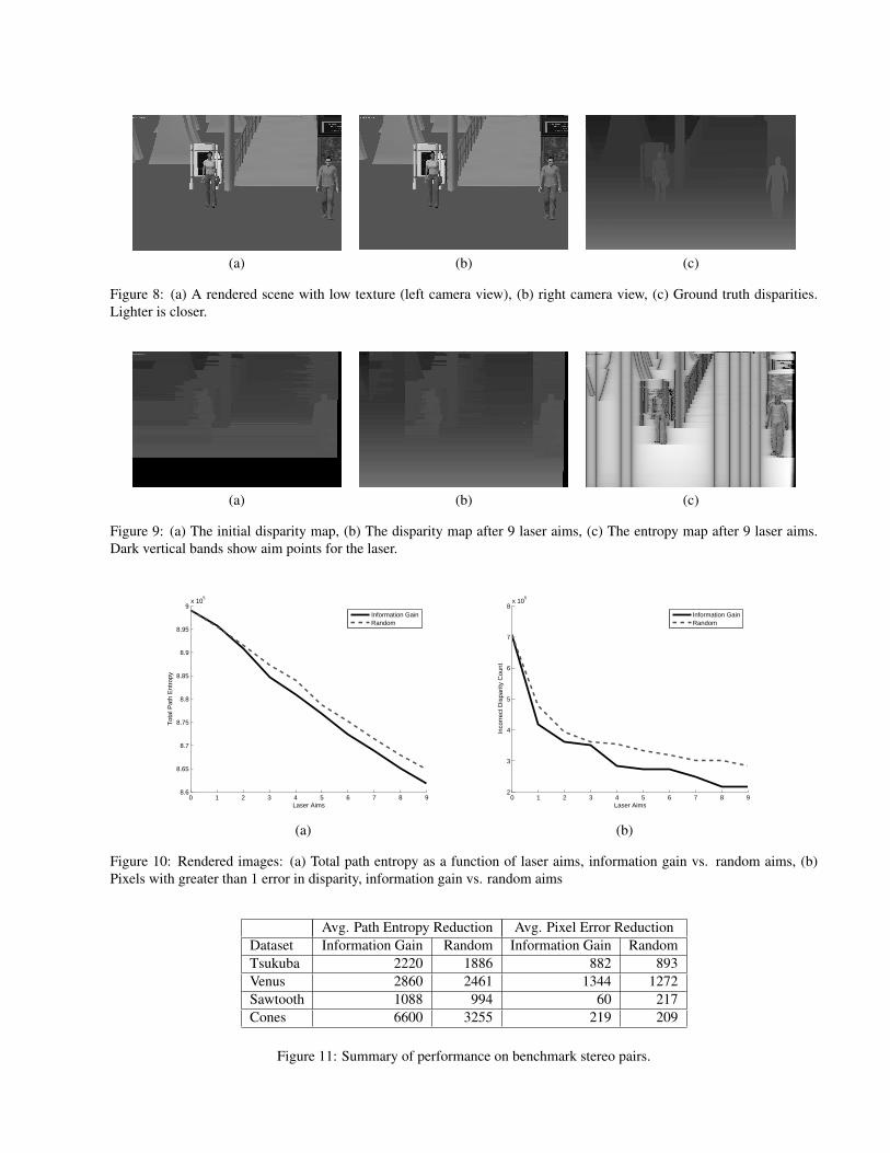
In our first set of synthetic experiments, we used a ren-dered pair of 1256 × 810 images (Figure 8 a,b) that wereintentionally created with low texture information. Groundtruth data were available from the rendering program andthese were used to simulate laser lines. Figure 8c showsthe ground truth disparity map for this image pair. Fig-ure 9a shows the initial disparity map from the stereo al-gorithm. A disparity map shows pixel disparities as lumi-nance. Higher disparities correspond to closer depths andhigher luminance in the disparity map. Notice the the floorclose to the camera is totally wrong due to the lack of tex-ture information. Figure 9b shows the disparity map after9 laser aims and Figure 9c shows the entropy map after 9laser aims. The entropy map is like the disparity map, butshows areas of high entropy (in the marginal distribution)with higher luminance. The dark vertical bands show laseraim points, in which the entropy has been forced to zero.The algorithm has chosen the areas of low texture that willhave the greatest expected reduction in total path entropy.

To help quantify the effect of our laser aiming strategy,we provide two graphs. In Figure 10a, we show the totalpath entropy through the DSI as a function of the numberof laser aims and in Figure 10b, we show the number ofpixels with disparity errors greater than 1. In both caseswe compare against an average of 10 random laser aims.Random aims can, initially, do well in this image because

nearly anything helps resolve the large, ambiguous floorarea close to the camera. However, our strategy of max-imizing expected information gain establishes a growinglead after the first few aims.

3.2 Benchmark Images

We performed experiments on several of the benchmarkimages from the Middlebury stereo vision suite [7]. Webriefly present some results for several of these images inFigure 11. Maximizing information gain generally out-performs random aims for entropy reduction, although thebenefit is not always large. For pixel error (the number ofpixels off by more than 1 disparity value), there is no con-sistent advantage to maximizing information gain - at leastfor a horizon of 9 laser aims. Neither of these results areunexpected. These benchmark images are well textured tostart with, so adding additional texture, no matter how wellplanned, will have limited benefit. Since our algorithm di-rectly optimizes information gain, we would expect it toperform best for entropy reduction, which doesn’t neces-sarily imply short term improvements in pixel error. Forexample, the laser aims could serve to confirm choices thatwere (fortuitously) correct in the Viterbi matching withouthaving much impact on the pixel error.

4 Physical Implementation andExperiments

To test our algorithm on a realistic scenario more similar towhat a robot would actually encounter, we built a prototypesystem (Figure 12a) and moved it into the hallway of ourdepartment (Figure 12b). The prototype system consistedof two consumer digital SLR cameras attached to a tripod,a computer controlled pan/tilt head connected to a separatetripod, and a consumer green laser pointer with an inexpen-

(a) (b) (c)

Figure 8: (a) A rendered scene with low texture (left camera view), (b) right camera view, (c) Ground truth disparities.Lighter is closer.

(a) (b) (c)

Figure 9: (a) The initial disparity map, (b) The disparity map after 9 laser aims, (c) The entropy map after 9 laser aims.Dark vertical bands show aim points for the laser.

0 1 2 3 4 5 6 7 8 98.6

8.65

8.7

8.75

8.8

8.85

8.9

8.95

9x 10

5

Laser Aims

Tot

al P

ath

Ent

ropy

Information GainRandom

0 1 2 3 4 5 6 7 8 92

3

4

5

6

7

8x 10

5

Laser Aims

Inco

rrec

t Dis

parit

y C

ount

Information GainRandom

(a) (b)

Figure 10: Rendered images: (a) Total path entropy as a function of laser aims, information gain vs. random aims, (b)Pixels with greater than 1 error in disparity, information gain vs. random aims

Avg. Path Entropy Reduction Avg. Pixel Error ReductionDataset Information Gain Random Information Gain RandomTsukuba 2220 1886 882 893Venus 2860 2461 1344 1272Sawtooth 1088 994 60 217Cones 6600 3255 219 209

Figure 11: Summary of performance on benchmark stereo pairs.

sive beam spreading lens attached to the front. The entireapparatus was connected to a laptop. The apparatus mayappear a bit bulky but this is largely due to some choicesthat were made to permit faster prototyping. A real systemon a robot could use smaller cameras and a less advancedpan/tilt unit since high pan/tilt accuracy is not critical forour application.

The cameras were carefully calibrated before the experi-ments, but the only calibration of the laser was some handadjustment to ensure that it looked approximately verticalin the right frame. We performed laser detection with im-age subtraction and some simple heuristics.

We generated a “ground truth” disparity map by producingapproximately 200 laser aims and using stereo vision to fillin the gaps between the laser aims. The data collectiontook approximately 90 minutes of real time and the resultsare shown in Figure 12c. The disparity map matches ourpersonal knowledge of the scene quite well. The differencebetween this and the initial disparity map shown in Fig-ure 13a is striking, due to the textureless walls. The initialdisparity map interprets the slanted wall as a collection ofpanels parallel to the image plane, separated by changes inluminance. This is a common artifact of stereo algorithms.

We applied our entropy minimization strategy to the dataset collected in our own hallway. The images with 200laser aims were treated as ground truth and queries weresatisfied by returning the closest of the 200 laser aims to therequest made by the algorithm. The results of these runs,compared to random laser aims, and evenly spaced laseraims are shown in Figure 15. As expected, entropy min-imization significantly outperforms the alternatives whenthe performance criterion is the reduction in path entropy.In the short term, entropy minimization does not seem toperform well at pixel error reduction, but it appears that thecumulative effect of entropy reduction pays off with morelaser aims, as seen on the right hand side of Figure 15b.The corresponding disparity maps are shown in Figure 13b,c. While the disparity map still isn’t perfect, the effectof 9 laser aims is a substantial improvement. Figure 14 a-cshows the entropy maps before and after laser aims. Theaim points chosen by the algorithm correspond well withweakly textured, highly ambiguous areas of the image.

5 Related Work

It is not uncommon in the stereo vision literature for match-ing costs to be interpreted as probabilities [2, 5, 4, 9]. How-ever, such interpretations are typically seen primarily asjustifications for various optimization techniques. The useof structured light sources from a projector is also a fairlywell established technique [8].

The observations made by Anderson and Moore [1] aremost relevant to our information gain computation, but the

work of Guestrin and Kraus [6], which considers optimalnonmyopic information gathering actions is also highlyrelevant. Unfortunately, the algorithms presented in thatwork, while polynomial for structures like ours, are stilltoo slow for real time use. For a large image, anythingmore than O(nd), even O(nd2), is impractical since d canbe quite large (hundreds of pixels).

Our work can be viewed as one of the first that uses theprobabilistic interpretation of stereo matching costs forsome purpose other than match cost optimization. We offerthe first probabilistic interpretation of the Bobick and Intillealgorithm, generalize this algorithm to compute marginalprobabilities and entropies efficiently, and apply insightsfrom graphical models to compute the information gain ef-ficiently.

6 Future Work

A most important practical direction for future work is thefull deployment of this technique on a robot. This wouldmost likely entail the use of some compact cameras and asimpler pan tilt mechanism to reduce overall bulk. Oncethis is accomplished, we would like to integrate the newsensor into a vision based mapping algorithm.

For the sensor itself, there are several interesting directionsfor future work. First, our algorithm uses a laser line, buta laser line may not be practical in all cases. Due to eyesafety concerns, it may not always be possible to use a laserpowerful enough to generate a line that is spans the entirevertical field of view and is visible in bright light. A naturalsolution is to use a beam spreader with narrower dispersionand to use the tilt feature of a pan/tilt head to choose howto aim the laser line segment vertically. This is a fairlystraightforward generalization of our approach which canbe achieved quite efficiently.

From the algorithmic standpoint, another practical consid-eration is that total path entropy may not be the best cri-terion to optimize. Initially, it was a choice of (computa-tional) convenience. We are investigating if other criteriacan be computed as efficiently in some cases. We are alsointerested in the case where some regions of the image areidentified as more important than others and the optimalitycriterion is weighted accordingly.

Another direction for exploration would be the use of amore sophisticated stereo model. A natural fit would be thebelief propagation approach [9]. However, it is not guar-anteed that using a more sophisticated stereo model wouldbe worth the challenges involved, since the algorithm it-self would be significantly slower and it would be difficultor impossible to compute the information gain efficiently.While a more sophisticated stereo model could in turn pro-vide better probabilities that could provide better guidancefor a laser aiming strategy, it could not fully resolve the fun-

(a) (b) (c)

Figure 12: (a) Our prototype camera/laser apparatus, (b) Our hallway, (c) Disparity map after 200 laser aims.

(a) (b) (c)

Figure 13: Hallway: (a) The initial disparity map, (b) The disparity map after 2 laser aims, (c) The disparity map after 9laser aims.

(a) (b) (c)

Figure 14: Hallway: (a) The initial entropy map, (b) The entropy map after 2 laser aims, (c) The entropy map after 9 laseraims. Gaps in the vertical lines from the laser can be due to occlusions or areas where the laser could not be detected withhigh confidence.

0 1 2 3 4 5 6 7 8 97.4

7.6

7.8

8

8.2

8.4

8.6

8.8x 10

5

Laser Aims

Tot

al P

ath

Ent

ropy

Information GainRandomRegular Intervals

0 1 2 3 4 5 6 7 8 94.1

4.2

4.3

4.4

4.5

4.6

4.7x 10

5

Laser Aims

Inco

rrec

t Dis

parit

y C

ount

Information GainRandomRegular Intervals

(a) (b)

Figure 15: Hallway: (a) Total path entropy vs. number of laser aims, (b) Pixels off by more than one disparity value vs.laser aims

damental ambiguity posed by textureless surfaces withoutmaking some strong, additional assumptions. While thisdirection is worth exploring, it could turn out that using asimpler stereo algorithm is more efficient overall.

Finally, a less glamorous but no less important area for fur-ther study is the choice of parameters for the algorithm.This is an issue for stereo algorithms in general and it ismore of a concern for our approach. In addition to the oc-clusion penalties, we must choose a scaling factor whenconverting scores to potentials. The choice of scaling fac-tor can make the distribution over paths more or less peakedand can alter the behavior of the algorithm. Different sizeimages appear to require different parameters and a prin-cipled method for determining these parameters would bea significant improvement over our ad hoc search for goodvalues.

7 Conclusions

We have addressed the challenge of active stereo visionusing an entropy minimization approach. By adopting aprobabilistic interpretation of an existing O(nd) stereo al-gorithm and adapting this algorithm to compute probabil-ities and entropies, we have devised an approach to se-lecting the action with the greatest information gain thatis, asymptotically, no more expensive than the core stereoalgorithm. This is critical for the stereo problem becauseeven a quadratic cost in the maximum disparity can be ex-tremely large for high resolution images.

Our approach to this problem leverages a probabilistic in-terpretation of the stereo problem and employs insightsgained from recent work probabilistic reasoning for sensormanagement.

We have implemented this algorithm and shown that itmakes good choices of laser aim points in simulation of ahybrid stereo vision/laser device. We have also built thisdevice and demonstrated that it can be used to producehigh resolution disparity maps of real scenes. We are ac-tively pursuing this approach as a practical alternative toprohibitively expensive and bulky three dimensional laserrange finders.

Acknowledgment

We are grateful to Carlo Tomasi for many helpful sugges-tions. The rendered image used in our synthetic experi-ments was provided by IAI. This work was supported byNSF IIS award 0209088, SAIC, and the Sloan Foundation.

References

[1] Brigham Anderson and Andrew Moore. Active learn-ing for hidden markov models: Objective functions and

algorithms. In Proceedings of the twenty second inter-nation conference on machine learning, 2005.

[2] Peter N. Belhumeur and David Mumford. A Bayesiantreatment of the stereo correspondence problem usinghalf-occluded regions. In IEEE Computer Society In-ternational Conference on Computer Vision and Pat-tern Recognition, pages 506–512, June 1992.

[3] A. F. Bobick and S. S. Intille. Large occlusion stereo.Int. J. Comput. Vision, 33(3):181–200, 1999.

[4] I. J. Cox, S. L. Hingorani, S. B. Rao, and B. M. Maggs.A maximum likelihood stereo algorithm. Computer Vi-sion and Image Understanding, 63(3):542–567, May1996.

[5] Davi Geiger, Bruce Ladendorf, and Alan Yuille. Oc-clusions and binocular stereo. International Journal ofComputer Vision, 14(3):211–226, April 1995.

[6] A. Kraus and C. Guestrin. Optimal nonmyopic valueof information in graphical models efficient algorithmsand theoretical limits. In Proceedings of the Nine-teenth International Joint Conference on Artificial In-telligence (IJCAI), 2005.

[7] D. Scharstein and R. Szeliski. A taxonomy and eval-uation of dense two-frame stereo correspondence al-gorithms. International Journal on Computer Vision,47(1/2/3):7–42, April–June 2002.

[8] Daniel Scharstein and Richard Szeliski. High-accuracystereo depth maps using structured light. In CVPR (1),pages 195–202, 2003.

[9] J. Sun, H. Y. Shum, and N. N. Zheng. Stereo matchingusing belief propagation. In Proc. European Confer-ence on Computer Vision, pages 510–524, 2002.