Efﬁcient Evaluation of the Valid-Time Natural Join

34Efficient Evaluation of the Valid-Time

Natural JoinMichael D. Soo, Richard T. Snodgrass, and

Christian S. Jensen

Joins are arguably the most important relational operators. Poor implementa-tions are tantamount to computing the Cartesian product of the input relations.In a temporal database, the problem is more acute for two reasons. First, con-ventional techniques are designed for the optimization of joins with equalitypredicates, rather than the inequality predicates prevalent in valid-time queries.Second, the presence of temporally-varying data dramatically increases the sizeof the database. These factors require new techniques to efficiently evaluatevalid-time joins.

We address this need for efficient join evaluation in databases support-ing valid-time. A new temporal-join algorithm based on tuple partitioning isintroduced. This algorithm avoids the quadratic cost of nested-loop evalua-tion methods; it also avoids sorting. Performance comparisons between thepartition-based algorithm and other evaluation methods are provided. While wefocus on the important valid-time natural join, the techniques presented are alsoapplicable to other valid-time joins.

1109

1110 IMPLEMENTATION TECHNIQUES

1 Introduction

Time is an attribute of all real-world phenomena. Consequently, efforts to incorpo-rate the temporal domain into database management systems (DBMSs) have beenon-going for more than a decade [22, 24, 23]. The potential benefits of this researchinclude enhanced data modeling capabilities, and more conveniently expressed andefficiently processed queries over time.

Whereas past work in temporal databases has concentrated on conceptual is-sues such as data modeling and query languages, recent attention has focused onimplementation-related issues, most notably indexing and query processing strate-gies. We consider in this paper an important subproblem of temporal query pro-cessing, the evaluation of temporal join operations.

Joins are arguably the most important relational operators. They occur fre-quently due to database normalization and are potentially expensive to compute.Poor implementations are tantamount to computing the Cartesian product of theinput relations. In a temporal database, the problem is more acute. Conventionaltechniques are aimed towards the optimization of joins with equality predicates,rather than the inequality predicates prevalent in temporal queries [15]. Secondly,the introduction of a time dimension may significantly increase the size of the data-base. These factors require new techniques to efficiently evaluate valid-time joins.

Valid-time databasessupportvalid-time, the time when facts were true in thereal-world [20, 8]. In this paper, we consider strategies for evaluating thevalid-timenatural join [2, 16], which matches tuples with identical attribute values duringcoincident time intervals. Other terms for the valid-time natural join include thenatural time-join[2] and thetime-equijoin(TE-join) [6]. Like its snapshot coun-terpart, the valid-time natural join supports the reconstruction of normalized data[11]. Efficient processing of this operation can greatly improve the performance ofa database management system.

Join evaluation algorithms fall into three basic categories, nested-loop, sort-merge, or partition-based [19]. The majority of previous work in temporal joinevaluation has concentrated on refinements of the nested-loop [21, 6] and sort-merge algorithms [15]. Comparatively little attention has been paid to partition-based evaluation of temporal joins, the notable exception being Leung and Muntzwho considered such algorithms in a multiprocessor setting [18].

In this paper, we present a partition-based evaluation algorithm for valid-timejoins that clusters tuples with similar validity intervals. If the number of disk pagesoccupied by the input relations isn then, in terms of I/O costs, our algorithm allowsanO(n) evaluation cost in many situations, thereby improving on theO(n2) costof nested-loop evaluation and theO(n · log(n)) cost of sort-merge evaluation. In

EFFICIENT EVALUATION OF THE VALID-TIME NATURAL JOIN 1111

addition, our approach does not require sort orderings or auxiliary access paths,each with additional update costs, and adapts easily to an incremental evaluationframework [25].

The paper is organized as follows. Section 2 formally defines the valid-timenatural join in a common representational data model that is well-suited for queryevaluation. A new, partition-based algorithm for computing the valid-time naturaljoin is presented in Section 3. Performance comparisons between the partition-based algorithm and previous valid-time join evaluation algorithms are made inSection 4. Conclusions and future work are detailed in Section 5.

2 Valid-Time Natural Join

In this section, we define the valid-time natural join using the tuple relational cal-culus. The definition we provide is for a 1NF tuple-timestamped data model. Anequivalent definition for a conceptual-level data model [12, 13] is given elsewhere[25].

In the data model, tuples are stamped with intervals denoting their time ofvalidity. We assume that the time-line is partitioned into minimal-duration intervals,termedchronons[5]. Timestamps are therefore single intervals denoted by inclusivestarting and ending chronons.

LetR andS be valid-time relation schemas

R = (A1, . . . , An, B1, . . . , Bk,Vs,Ve)

S = (A1, . . . , An, C1, . . . , Cm,Vs,Ve)

where theAi , 1≤ i ≤ n, are the explicit join attributes, theBi , 1≤ i ≤ k, andCi ,1 ≤ i ≤ m, are additional, non-joining attributes, and Vs and Ve are the valid-timestart and end attributes. We use V as a shorthand for the interval[Vs,Ve]. Also, wedefiner ands to be instances ofR andS, respectively.

In the valid-time natural join, two tuplesx andy join if they satisfy the snap-shot equi-join condition (i.e., they match on the explicit join attributes), and if theyhave overlapping valid-time intervals. The attribute values of the resulting tuplez

are as in the snapshot natural join, with the addition that the valid-time interval isthe maximal overlap of the valid-time intervals ofx andy. We formalize this withthe following definitions.

Definition 1 The functionoverlap(U, V ) returns the maximal interval containedin both of the intervalsU andV . We provide a procedural definition ofoverlap.The auxiliary functionsmin andmax return the smallest chronon and largest chro-nons, respectively, in their argument sets.


overlap(U ,V ):common← ∅;for each chronont fromUs toUe

if Vs ≤ t ≤ Ve common← common∪ {t};if common = ∅ result ←⊥;else result ← [min(common),max(common)];returnresult ; 2

Definition 2 The valid-time natural join ofr ands, r 1V s, is defined as follows.

r 1V s = {z(n+m+k+2) | ∃x ∈ r ∃y ∈ s(x[A] = y[A] ∧ z[A] = x[A]∧z[B] = x[B] ∧ z[C] = y[C]∧z[V] = overlap(x[V], y[V])∧ z[V] 6=⊥)} 2

3 Valid-Time Partition Join

In this section, we show how partitioning can be used to evaluate the valid-timenatural join. We begin by describing, in Section 3.1, the general characteristics ofpartition joins. In Sections 3.2 to 3.4, we show how valid-time can be supported ina partition-based framework.

3.1 Overview of Partition Joins

Partition joinscluster tuples with similar join attribute values, thereby reducing theamount of unnecessary comparison needed to find matching tuples [19]. Both inputrelations are partitioned so that tuples in a particular partition of one relation canonly match with tuples in a corresponding partition of the other relation. A primarygoal is to perform the partitioning so that joins between corresponding partitionscan be efficiently evaluated.

Partition-join evaluation consists of three phases. First, the attribute valuesdelimiting partition boundaries are determined. The partition boundaries are chosento minimize the evaluation cost—disk I/O is usually the dominant factor. Second,these attribute values are used to physically partition the input relations. In theideal case, this involves linearly scanning both input relations and placing tuplesinto the appropriate partition. Lastly, the joins of corresponding partitions of theinput relations are computed. In the ideal case, the partitions are small enough to fitin the available main memory and can be accessed with a single random disk seekfollowed by relatively inexpensive sequential reads. Ignoring the cost of operationsperformed in main memory, any simple evaluation algorithm, such as nested-loopsor sort-merge, can be used to join the partitions once in memory. If the partitioningsatisfies the given buffer constraints, the join can be computed with a linear I/Ocost, thereby avoiding the quadratic complexity of the brute force implementation.


Figure 1 shows how partitioning is used to computer 1 s for two snapshotrelationsr ands. Relationsr ands are initially scanned and tuples are placed intopartitionsri andsi , 1 ≤ i ≤ n, depending on their joining attribute values. Thepartitioning guarantees that, for any tuplex ∈ ri , x can only join with tuples insi .The result,r 1 s, is produced by unioning the joinsri 1 si .

↓ ↓ ↓↓

1 1 1 1

r1 r2 r3 rn

s1 s2 s3 sn

r1 1 s1 r2 1 s2 r3 1 s3 rn 1 sn

· · ·

· · ·

· · ·

Figure 1: Partition Join ofr 1 s

Suppose thatbuffSizepages of buffer space are available in main memory. If apartitionri occupiesbuffSize−2 pages or less then it is possible to computeri 1 siby readingri into main memory and joining it with each page ofsi one at a time.(The remaining page of main memory is used to hold result tuples.) Therefore,a single linear scan ofr ands suffices to computer 1 s. Also, the partitioningprovides a natural clustering mechanism on tuples with similar attribute values. Ifpartitions are stored on consecutive disk pages then, after an initial disk seek to thefirst page of a partition, its remaining pages are read sequentially. Last, it is easyto see how the algorithm can be adapted to an incremental mode of operation. Forexample, suppose thatr 1 s is materialized as a view, and an update happens tor

in partitionri . As tuples inri can only join with tuples insi , the consistency of theview is insured by recomputing onlyri 1 si .

3.2 Supporting Valid-Time

We now present a partition-join algorithm to compute the valid-time natural joinr 1V s of two valid time relationsr ands in the tuple-timestamped representationof Section 2.


Our approach is to partition the input relations using a tuple’s interval of va-lidity. For the corresponding partitionsri andsi , the partitioning guarantees that foreachx ∈ ri , x can only join with tuples insi , and, similarly,y ∈ si can join onlywith tuples inri .

Tuple timestamping with intervals adds an interesting complication to the par-titioning problem. Since tuples can conceivably overlap multiple partitions, thesetuples, termedlong-lived tuples, must be present in each partition they overlap whenthe join of that partition is being computed. That is, the tuple must be present inmain memory when the join of an overlapping partition is being computed. Noticethat this problem does not occur in the partition join of snapshot relations since, ingeneral, the joining attributes are not range values such as intervals.

A straightforward solution to this problem simply replicates the tuple acrossall overlapping partitions [18]. However, replication requires additional secondarystorage space and complicates update operations.

We propose a different solution that guarantees the presence of the tuple ineach overlapping partition when the join of that partition is computed, while avoid-ing replication of the tuple in secondary storage. Simply, we choose a single over-lapping partition to contain the tuple on disk and dynamically migrate the tuple tothe remaining partitions as the join is being evaluated.

The evaluation algorithm is shown in Figure 2. As with partition-join algo-rithms for conventional databases, three steps are performed. First, the attributevalues that determine partition boundaries are determined. This is performed byproceduredeterminePartIntervals. Next the relations are partitioned by proceduredoPartitioning, and lastly, the partitioned relations are joined by procedurejoinPar-titions.

partitionJoin(r, s):partIntervals←

determinePartIntervals(buffSize, |r|, |s|);r ← doPartitioning(r, partIntervals);s ← doPartitioning(s, partIntervals);returnjoinPartitions(r, s, partIntervals);

Figure 2: Evaluation ofr 1V s

We assume that Grace partitioning [14, 19] is used in proceduredoPartition-ing. We reserve a single buffer page to hold a page of the input relation, and dividethe remaining buffer space evenly among the partitions. Each tuple inr ands is ex-amined and placed in a page belonging to the appropriate partition; when the pagesfor a given partition become filled they are flushed to disk. We assume that thenumber of partitions is small, and therefore, that sufficient main memory is avail-


able to perform the partitioning. This assumption held true for all experiments weperformed. As partitioning is straightforward, we concentrate on the remaining al-gorithms. The following section describes how two partitioned relations are joinedin procedurejoinPartitions. For the time being, we assume thatr ands are dividedinto n equal sized partitions and postpone until Section 3.4 the details of proceduredeterminePartIntervals.

3.3 Joining Partitions

Let P be a partitioning of valid time, i.e.,P is a set ofn non-overlapping intervalspi , 1 ≤ i ≤ n, that completely covers the valid-time line. Associated with eachpiis a partitionri of r. We assume, for the purposes of this section, that eachri hasapproximately the same number of tuples.

We assume that a tuplex is in the partitionri if and only if overlap(x[V], pi)6=⊥, and similarly fory ∈ si . Tuples are physically stored in the last partition theyoverlap, that is, a tuplex is physically stored in partitionri if overlap(x[V], pi) 6=⊥and¬∃j such thatj > i andoverlap(x[V], pj) 6=⊥.1 The computation proceedsfrom rn 1

V sn to r1 1V s1. For a givenri , all tuplesx ∈ ri that overlappi−1 are re-tained and added tori−1 prior to computingri−1 1

V si−1, and similarly forsi−1. Astuples are initially placed in their last overlapping partition, this algorithm ensuresthat tuples are present in each partition they overlap, and does so without introduc-ing unnecessary redundancy in secondary storage. Notice also that if a given tuplex overlaps partitionspj , . . . , pi−1, pi thenx must be present inrj , . . . , ri−1, riwhen their corresponding join is computed; therefore, no unnecessary comparisonsare performed.

The buffer allocation strategy used in this algorithm is shown in Figure 3.Space is allocated to hold an entire partitionri of the outer relationr, a page of thecorresponding partitionsi of the inner relation, a page, thetuple cache, to hold thelong-lived tuples ofs, and a page to hold the result tuples. For a detailed descriptionof the movement of tuples between the buffers, see Appendix A.1.

3.4 Partitioning Strategies

In the previous section, we described how the join of two previously partitioned re-lations was computed, assuming that each partition of the outer relationr, containedapproximately equal numbers of tuples. We show in this section how to determine apartitioning of the input relations that satisfies this property with relatively small I/O

1An equivalent strategy is to place tuples in their first partition and propagate long-lived tuples towards thelast partition during evaluation. We chose the given strategy with consideration for incremental adaptationsdescribed elsewhere [25].

1116

IMP

LEM

EN

TAT

ION

TE

CH

NIQ

UE

S

r

Tuple cache

s

Inner relationpage

Tuple cachepage

Result relationResult relationpage

Main memory

Outer relationpartition area

Figure 3: Buffer Allocation forr 1V s Evaluation


cost. Our method is inspired by the partition-size estimation technique originallydeveloped for the evaluation ofband-joins[4].

In Figure 3, a single buffer page is allocated to each of the inner relationbuffer, tuple cache, and result relation, andbuffSizepages are allocated to hold apartition of the outer relation. Our goal is to ensure that eachri fits in the availablebuffSizepages with high probability, while minimizing the I/O cost of ensuring thisimportant property.

The task at hand is to construct a set ofpartitioning intervalsthat coversthe valid-time line. Tuples belong to a partition if they overlap, in valid time, thecorresponding partitioning interval. Note that the length of a partitioning intervalpi determines the cardinality of the resulting partitionri .

A simple strategy to construct thepi is to sortr on Ve or Vs , and then choosethe partitioning chronons in a subsequent linear scan. While this yields an optimalsolution, it is prohibitively expensive.

A better solution is to choose partitioning intervals that with high probabilityare close to those that would have been chosen with the exact method. To do this,we randomly sample tuples fromr, and, based on this sample set, choose a set ofpartitioning chronons, from which the partitioning intervals are constructed. Asour partitioning is only approximate, some portion of thebuffSizepages must bereserved to accommodate errors in the chronon choices that would likely result inoverflow of the outer relation partition area. We note that should such errors occur,that is, a partition is created that is bigger thanbuffSizepages, the correctness of thejoin algorithm is not affected—only performance will suffer due to buffer thrashing.

Samples drawn from the outer relation are used to determine the intervals usedto partition both the outer and inner relations. In addition, this same sample set isused to estimate the caching costs associated with long-lived tuples in the innerrelation. We make the implicit assumption that the distribution, over valid time, oftuples in the outer and inner relations is similar, thereby allowing us to use a singlesample set for both purposes. We provide justification for this assumption later.

The cost of evaluatingr 1V s has the following three components (c.f., Fig-ure 2).

• Csample—the cost of samplingr,

• Cpartition—the cost of creating the partitionsri andsi , 1≤ i ≤ n, and

• Cjoin—the cost of joining the partitionsri andsi , 1≤ i ≤ n.

The total I/O costCtotal is the sum of these,

Ctotal = Csample + Cpartition + Cjoin.Our goal, then, is to choose a set of partitioning intervals so that the estimatedevaluation cost,Ctotal , is minimized. Since the cost of Grace partitioning is notaffected by the chosen partition size (it is dependent only on the amount of available


main memory), we need only consider the sumCsample + Cjoin. In the following,we show how to compute the set of partitioning intervals that minimizesCsample +Cjoin.

Let partSize≤ buffSizebe the estimated size of an outer relation partition. Wewant to find apartSizethat minimizesCsample + Cjoin. Let errorSize= buffSize− partSizebe the amount of buffer space available to handle overflow if a partitionexceeds the estimated size. IfpartSizeis large thenerrorSizeis small. The effectof a smallerrorSizeis to increaseCsample since, in order to prevent overflowingthe smaller error space, higher accuracy is needed when choosing the partitioningintervals. However, a largepartSizedecreasesCjoin since tuples are less likelyto overlap many partitions when the partitioning intervals are large, resulting ina decrease in tuple-cache paging. Alternatively, consider the effects of a smallpartSize, and, hence, largeerrorSize. Since more overflow space is available, fewersamples need to be drawn, andCsample decreases. However, the smallerpartSizeincreasesCjoin since tuples are more likely to overlap multiple partitions, if thepartitioning intervals are small.

In summary, a cost tradeoff occurs between the amount of sampling per-formed on the outer relation, a component ofCsample, and the amount of pagingperformed on the tuple cache, a component ofCjoin. The optimal solution mini-mizes the sumCsample + Cjoin.

Partition size

Cost

Csample

Cjoin

Csample Cjoin+

I/O

(partSize)

Figure 4: I/O Cost for Partition Size

Figure 4 plots sampling and tuple-cache paging costs for increasing partitionsizes. As seen from the figure, as the expected partition sizepartSizeincreases,sampling costs (Csample) increase monotonically and tuple-cache paging costs (and


henceCjoin) decrease monotonically. In order to minimize the evaluation cost, thesum of the sampling cost and the tuple-cache paging cost (shown as a dotted line inthe figure) must be minimized.

This minimal sum is determined by computing, given the buffer constraintbuffSize, Csample + Cjoin for each possiblepartSize. If few long-lived tuples arepresent inr then the tuple-cache paging cost will decrease very quickly, and theminimal cost will be obtained at a larger partition size. Conversely, if many long-lived tuples are present inr then the tuple-cache paging cost will decrease slowly,and the minimal cost will be obtained at smaller partition sizes.

The number of samples to draw is determined using the Kolmogorov teststatistic [3, 4]. The Kolmogorov test is a non-parametric test which makes noassumptions about the underlying distribution of tuples. With 99% certainty, thepercentile of each chosen partitioning chronon will differ from an exactly cho-sen partitioning chronon by at most 1.63/

√m, wherem is the number of samples

drawn fromr [3]. Since 1.63/√m represents a percentage difference from an ex-

act partitioning, we know that(1.63× |r|)/√m is the number of necessary errorpages should a partition overflow the allottedpartSizepages. Hence, we must have(1.63× |r|)/√m ≤ errorSizewhich implies thatm ≥ ((1.63× |r|)/errorSize)2

samples must be drawn.2

The algorithmdeterminePartIntervals, shown in Appendix A.2, determines,for a givenbuffSize, thepartSizethat minimizesCsample+Cjoin. The correspondingset of partitioning intervals is returned as its result. It uses an additional procedurechooseIntervals, shown in Appendix A.3 that chooses partitioning intervals froma set of partitioning chronons.

From the sample set, and its derived partitioning, the tuple cache paging costsare estimated. For a given partition, the estimated size of its tuple cache is the num-ber of sampled tuples that overlap its partitioning interval scaled by the percentageof the relation sampled. This simple strategy suffices since accurately estimatingthe amount of tuple cache paging is not as critical as estimating the size of the outerrelation partition. Partitions are large; therefore, rereading of partitions will incura large expense. However, for any given partition, the size of its tuple cache issmall, being bounded by the partition size; for many applications the tuple cachewill contain a relatively small percentage of the partition. The expense of apply-ing a sophisticated technique such as the Kolmogorov test, or directly sampling theinner relation, is not justified.

The algorithmestimateCacheSizes, shown in Appendix A.4, performs thetuple cache size estimation described here.

2It is interesting to note that the number of samples required is independent of|r|. SinceerrorSizeis somenumber of pages we can expresserrorSizeas a percentage of|r|, errorSize= |r|/l, wherel is some integer.Substituting this expression forerrorSizeinto the formula form yields an expression independent of|r|.


4 Performance

In this section, we describe performance experiments involving the partition-joinalgorithm. We first describe, in Section 4.1, previous work in valid-time join eval-uation and the general setting for the experiments. Sections 4.2 to 4.4 describe indetail the experiments we performed. Conclusions are offered in Section 4.5.

4.1 General Considerations

A wide variety of valid-time joins have been defined, including thetime-join, event-join, TE-outerjoin[21], contain-join, contain-semijoin, intersect-join, overlap-join[17], andcontain-semijoin[16]. Refinements to the nested-loops algorithm wereproposed by Gunadhi and Segev to evaluate several temporal join variants [21, 7].This work assumed that temporal data was “append-only,” i.e., tuples are inserted intimestamp order into a relation, and once inserted into a relation are never deleted.With the append-only assumption, a new access path, theappend-only tree, wasdeveloped that provides a temporal index on the relation. Simple extensions tosort-merge were also considered where, again, tuples were assumed to be insertedinto a relation in timestamp order [21, 7]. Leung and Muntz extended this workto accommodate additional temporal join predicates, mainly those defined by Allen[1], and to incorporate various ascending and descending sort orders on either valid-start or valid-end time [15].

Simply stated, our work differs from most previous work in that we adaptthe third and remaining join evaluation strategy, partitioning, to the evaluation ofvalid-time joins. Our approach does not require sort orderings or auxiliary accesspaths, each with additional update costs, and it adapts easily to an incremental eval-uation framework. Partition-based evaluation of valid-time joins was investigatedby Leung and Muntz in the context of parallel join evaluation, but their strategyrequired the replication of tuples across processors. We avoided replication for tworeasons: to save on secondary storage costs and to easily adapt the algorithm to anincremental framework.

In order to evaluate the relative performance of our algorithm, we imple-mented main-memory simulations of partition join and sort-merge join, and calcu-lated analytical results for nested-loops join. To obtain a fair comparison, we madethe weakest assumptions possible about the input relations. That is, we do not as-sume any sort ordering of input tuples, nor the presence of additional data structuresor access paths, where the incremental cost of maintaining a sort order or an accesspath is hidden from the query evaluation. However, the sort-merge algorithm wasoptimized to make best use of the available main memory size, and similar remarksapply to the analytical results generated for nested-loops. We measured cost as thenumber of I/O operations performed by an algorithm, distinguishing between the


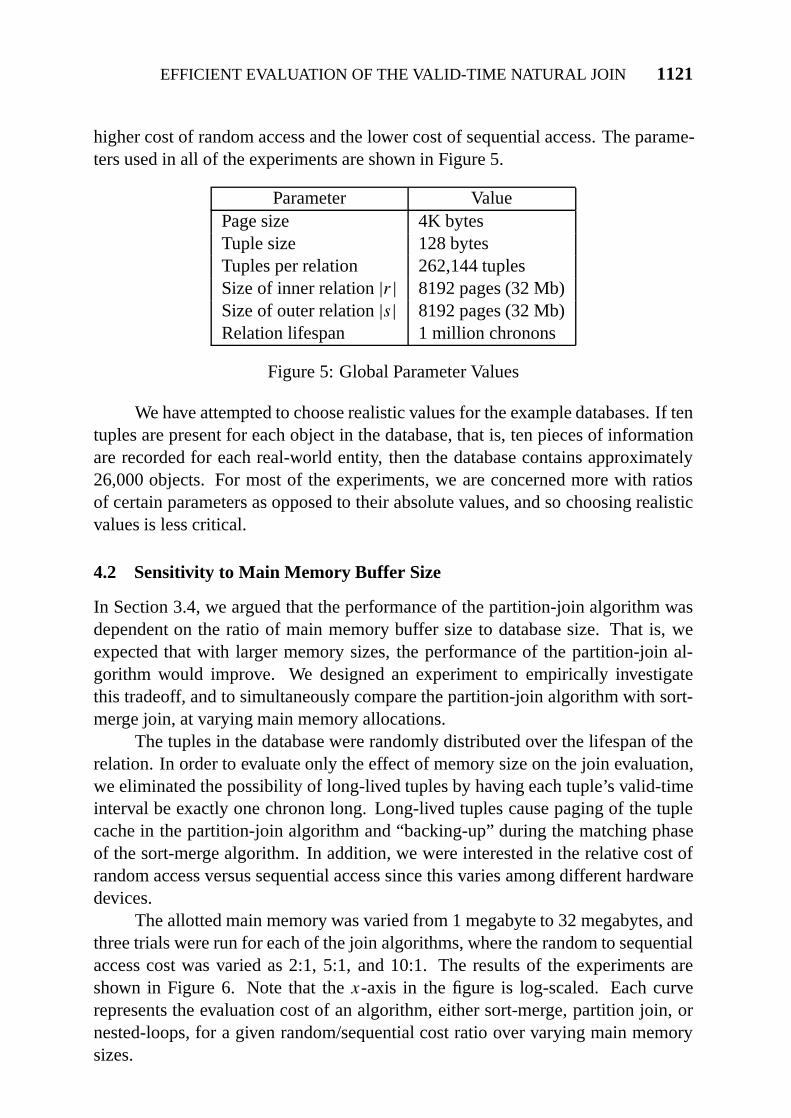
higher cost of random access and the lower cost of sequential access. The parame-ters used in all of the experiments are shown in Figure 5.

Parameter ValuePage size 4K bytesTuple size 128 bytesTuples per relation 262,144 tuplesSize of inner relation|r| 8192 pages (32 Mb)Size of outer relation|s| 8192 pages (32 Mb)Relation lifespan 1 million chronons

Figure 5: Global Parameter Values

We have attempted to choose realistic values for the example databases. If tentuples are present for each object in the database, that is, ten pieces of informationare recorded for each real-world entity, then the database contains approximately26,000 objects. For most of the experiments, we are concerned more with ratiosof certain parameters as opposed to their absolute values, and so choosing realisticvalues is less critical.

4.2 Sensitivity to Main Memory Buffer Size

In Section 3.4, we argued that the performance of the partition-join algorithm wasdependent on the ratio of main memory buffer size to database size. That is, weexpected that with larger memory sizes, the performance of the partition-join al-gorithm would improve. We designed an experiment to empirically investigatethis tradeoff, and to simultaneously compare the partition-join algorithm with sort-merge join, at varying main memory allocations.

The tuples in the database were randomly distributed over the lifespan of therelation. In order to evaluate only the effect of memory size on the join evaluation,we eliminated the possibility of long-lived tuples by having each tuple’s valid-timeinterval be exactly one chronon long. Long-lived tuples cause paging of the tuplecache in the partition-join algorithm and “backing-up” during the matching phaseof the sort-merge algorithm. In addition, we were interested in the relative cost ofrandom access versus sequential access since this varies among different hardwaredevices.

The allotted main memory was varied from 1 megabyte to 32 megabytes, andthree trials were run for each of the join algorithms, where the random to sequentialaccess cost was varied as 2:1, 5:1, and 10:1. The results of the experiments areshown in Figure 6. Note that thex-axis in the figure is log-scaled. Each curverepresents the evaluation cost of an algorithm, either sort-merge, partition join, ornested-loops, for a given random/sequential cost ratio over varying main memorysizes.


0

100000

200000

300000

400000

500000

600000

1 2 4 8 16 32

I/O T

ime

Main Memory (Megabytes)

Nested-Loops (10,5,2:1)Sort-Merge (10:1)Sort-Merge (5:1)Sort-Merge (2:1)

Partition Join (10,5,2:1)

Figure 6: Performance Effects of Main Memory

The graph shows an interesting property of the partition-join algorithm. Incontrast to nested-loops and sort-merge, the partition-join algorithm shows rela-tively good performance at all memory sizes, and, as expected, the performance ofthe algorithm improves as memory increases. Nested loops performs quite poorlyat small memory allocations since few pages of the outer relation can be stored inmemory, requiring many scans of the inner relation. At large memory allocations,e.g., 32 megabytes, the performance of nested-loops is quite good since a large por-tion of the outer relation remains resident in memory reducing the number of scansof the inner relation. We note also that the cost of reading the outer relation is quitelow since ifi pages of the outer relation are read, this requires a single random readfollowed by ai − 1 sequential reads.

Comparing the partition join to sort-merge, we see that the partition join isapproximately twice as fast as sort-merge at all memory sizes. As no backing up isperformed by the sort-merge algorithm, we attribute this to the cost of sorting. Atsmall memory sizes, the sort-merge algorithm must use more runs with fewer pagesin each run, with a random access required by each run.

Similarly, when little main memory is available, partition sizes are necessarilysmall, and higher random access cost is incurred by the partition-join algorithm dur-ing both the sampling and partitioning phases. That is, not only are more samplesrequired when the partitioning intervals are being determined, but, since less buffer


space is available, the in-memory “buckets” must be flushed more often, requiringmore random I/O. However, the effect on performance is not as drastic as for sort-merge since the partitioning phase requires only one pass through the relations, andwe discovered an optimization that can reduce sampling costs.

We initially assumed that a random access is required for each sample. Atlarge partition sizes, the effect is to perform a large number of random accessesduring sampling, sometimes exceeding the number of pages in the outer relation.The algorithm instead sequentially scans the outer relation, drawing samples ran-domly when a page of the relation is brought into main memory. For example, at arandom/sequential cost ratio of 10:1, only 819 random samples (3% of the relation)must be drawn before the entire outer relation can be scanned for the same cost.This requires only a single random access to read first page of the relation, followedby sequential reads of the remaining pages of the relation. The sampling cost istherefore proportional to the number of pages of the outer relation, as opposed tothe number of sampled tuples which may be quite large.

4.3 Effects of Long-Lived Tuples

The presence of long-lived tuples adds another cost dimension to both the partition-join and sort-merge algorithms. The partition-join algorithm may incur paging ofthe tuple cache when many long-lived tuples are present, and the sort-merge algo-rithm may back-up to previously processed pages of the input relations to matchoverlapping tuples. Long-lived tuples do not affect the performance of the nested-loops algorithm, but it is included here for completeness.

We designed an experiment to empirically investigate the cost effect that long-lived tuples have on both strategies. A series of databases were generated withincreasing numbers of long-lived tuples. Each database contained 32 megabytes(262144 tuples); we varied the number of long-lived tuples from 8000 to 128,000in 8000 tuple steps. Non-long-lived tuples were randomly distributed throughoutthe relation lifespan with a one chronon long validity interval. Long-lived tupleshad their starting chronon randomly distributed over the first 1/2 of the relationlifespan, and their ending chronon equal to the starting chronon plus 1/2 of the rela-tion lifespan. To not influence the performance of the algorithms via main memoryeffects, we fixed the main memory allocation at 8 megabytes, the memory size atwhich all three algorithms performed most closely in the previous experiment. Ad-ditionally, the random to sequential I/O cost ratio was fixed at 5:1. The results ofthe experiment are shown in Figure 7.

As can be seen from the figure, the partition-join algorithm outperformed thesort-merge algorithm at all long-lived tuple densities. We expected this result. Thetuple caching cost incurred by the partition-join algorithm is relatively low—thetuple cache size is small (it cannot exceed the size of a partition), and it is fairly


40000

50000

60000

70000

80000

90000

100000

110000

120000

130000

0 3 6 9 12 15 18 21 24 27 30 33 36 39 42 45 48

I/O Time

% of Long-Lived Tuples

Sort-MergeNested-Loops

Partition join

Figure 7: Performance Effects of Long-Lived Tuples

inexpensive to read or write (a random access for the first page followed by se-quential accesses for the remaining pages). Furthermore, many long-lived tuples donot significantly increase this cost since they merely cause additional pages to beappended to the tuple cache, and these pages incur an inexpensive sequential I/Ocost.

In contrast, the presence of long-lived tuples greatly increases the cost of thesort-merge algorithm. To see this, consider what happens when a long-lived tupleis encountered during the matching phase. The tuple must be joined with all tuplesthat overlap it, some of these tuples may, unfortunately, have already been read,requiring the algorithm to re-read these pages. For tuples with lifespans of 1/2 therelation lifespan, this incurs a significant cost. Furthermore, the percentage of long-lived tuples is less significant to the sort-merge algorithm. While a higher density oflong-lived tuples may require the algorithm to back-up more often, the presence ofonly a single long-lived tuple will still cause the sort-merge algorithm to back-up.

4.4 Main Memory vs. Long-Lived Tuples

The previous two experiments showed that the partition join exhibits better perfor-mance when more main memory is available, and incurs a performance penalty atincreasing densities of long-lived tuples.


We desired to determine whether the allotted main memory size or the densityof long-lived tuples played a larger effect on the performance of the partition-joinalgorithm, and designed an experiment to investigate this. Eight 262,144 tuple data-bases were generated with increasing numbers of long-lived tuples, from 16,000 to128,000 in 16,000 tuple steps. A trial was run for each database at 1, 2, 4, 16, and32 megabyte main memory allocations. The results are shown in Figure 8. (Thex-axis is log-scaled in the figure.)

30000

35000

40000

45000

50000

55000

60000

65000

70000

1 2 4 8 16 32

I/O T

ime

Main Memory (Megabytes)

128000 Long-Lived Tuples112000 Long-Lived Tuples96000 Long-Lived Tuples80000 Long-Lived Tuples64000 Long-Lived Tuples48000 Long-Lived Tuples32000 Long-Lived Tuples16000 Long-Lived Tuples

Figure 8: Relative Effects of Main Memory Size and Tuple Caching

The graph shows that at large memory sizes (16 and 32 megabytes) the eval-uation cost for all databases becomes fairly equal, hence the relative cost of tuplecaching is small due to the large memory size. At smaller memory sizes, there isa more pronounced difference between the evaluation costs over the different data-bases. This was expected. When the allotted memory sizes are small the cost oftuple caching is significant since partition sizes are necessarily smaller and moretuples are likely to overlap multiple partitions. Again, the conclusion to be drawnis that main memory availability is necessary for the partition join to be efficient.When sufficient main memory is available, the effects of tuple caching become in-significant, but when insufficient main memory is available, the performance impactof tuple caching is significant.


4.5 Summary

We expected that the partition-join algorithm would be sensitive to the amount ofmain memory available during evaluation. The experiment of Section 4.2 confirmsthis hypothesis. The algorithm performed better at larger memory sizes, mainlydue to the decreased random I/O during partitioning and the fewer samples requiredto determine the partitioning intervals. Furthermore, the partition join shows uni-formly good performance at all memory sizes, unlike nested-loops which performswell at large memory sizes, but quite poorly at small memory sizes.

Relative to sort merge, the partition-join algorithm compares favorably. Whenlong-lived tuples are present, the partition join outperforms sort-merge significantly,as shown in Section 4.3. Tuple caching in the partition join incurs a low cost relativeto the high cost of backing-up in sort-merge.

Finally, in Section 4.4, we compared the relative costs of tuple caching andmain memory availability. For the partition join, the density of long-lived tuples didnot greatly increase the evaluation cost when sufficient main memory was available.Given that sufficient main memory is available, our conclusion is that the partition-join algorithm performs well relative to both nested-loops and sort-merge, both inthe presence, and absence, of long-lived tuples.

5 Conclusions and Future Work

The contributions of this work are summarized as follows.

• We formally defined the valid-time natural join, the operator used to recon-struct normalized valid-time databases.

• We presented a new algorithm for valid-time join evaluation, improving ontheO(n2) cost of nested-loop join while avoiding theO(n · log(n)) cost ofsorting.

• Our approach is based on tuple partitioning, but still avoids replication oftuples in multiple partitions, thereby allowing simple base relation updates.

• We compared the performance of the partition-join algorithm with both nested-loop and sort-merge, and showed that with adequate main memory our algo-rithm exhibits almost uniformly better performance, especially in the presenceof long-lived tuples.

As relatively little work has appeared on temporal query evaluation, there aremany directions in which this work can be expanded. First, many important prob-lems remain to be solved with valid-time natural join evaluation. We made thesimplifying assumption in Section 3.4 that the distribution of tuples over valid timewas approximately the same for both the inner and outer relations. Obviously, thisassumption may not be valid for many applications since gross mis-estimation of


tuple caching costs may result. Secondly, while tuple caching is a relatively inex-pensive operation, the paging cost associated with it can be reduced if sufficientbuffer space is allocated to retain, with high probability, the entire tuple cache inmain memory. Trading off outer relation partition space for tuple cache space is apossible solution to this problem. Lastly, while we have distinguished between thehigher cost of random access and the lower cost of sequential access, we have ig-nored the cost of main-memory operations. Incorporating main-memory operationsinto the cost model would allow us to more accurately choose partitioning intervalsthrough better estimates of evaluation costs.

More globally, this work can be considered as the first step towards the con-struction of an incremental evaluation system for a bitemporal database manage-ment system, that is, a DBMS that supports both valid and transaction time [20, 8].Elsewhere we motivate the importance of incremental evaluation to temporal data-base management systems and show how our partition-based approach is easilyadapted to incremental evaluation [25].

Acknowledgements

Support for this work was provided the IBM Corporation through Contract #1124,the National Science Foundation through grants IRI-8902707 and IRI-9302244,and the Danish Natural Science Research Council through grant 11-9675-1 SE.We thank Nick Kline for providing the aggregation tree implementation used in thesimulations.

A Appendix

We describe in detail the algorithms used in Sections 3.3 and 3.4.

A.1 Algorithm joinPartitions

Algorithm joinPartitions, shown in Figure 9, computesr 1V s, assuming thatr ands have been previously partitioned. For eachi, 1≤ i ≤ n, the algorithm constructsthe next outer relation partitionri by purging tuples in the outer relation partitionbuffer that do not overlappi and reading in the physical partitionri from disk. riis then joined with the long-lived tuple cache. Tuples in the tuple cache that do notoverlappi−1 are purged afterri and the tuple cache are joined. We check this bycomparing a tuple’s validity interval with the partitioning intervals. Finally,ri isthen joined with each page ofsi . Tuples in the current page ofsi that overlappi−1

are inserted into the tuple cache to be available for the computation ofri−1 1V si−1.

In preparation for the next partition, tuples inri that overlappi−1 are retained in the


joinPartitions(r,s,partIntervals):cachePage← ∅;outerPart ← ∅;tupleCache← ∅;for i from n to 1

for each tuplex ∈ outerPartif overlap(x[V], partIntervalsi) =⊥

outerPart ← outerPart − {x};outerPart ← outerPart ∪ {read (ri)};resulti ← resulti ∪ outerPart 1V cachePage};for each tuplex ∈ cachePage

if overlap(x[V], partIntervalsi−1) 6=⊥newCachePage← newCachePage ∪ {x};

if filled(newCachePage)write(newCachePage);

for each flushed pagec of tupleCachecachePage← read (c);resulti ← resulti ∪ {outerPart 1V cachePage};for each tuplex ∈ cachePage

if overlap(x[V], partIntervalsi−1) 6=⊥newCachePage← newCachePage ∪ {x};

if filled(newCachePage)write(newCachePage);

for each pageo of siinnerPage← read (o);resulti ← resulti ∪ {outerPart 1V o};for each tuplex ∈ o

if overlap(x[V], partIntervalsi−1) 6=⊥newCachePage← newCachePage ∪ {x};if filled(newCachePage)

write(newCachePage);

returnresult1 ∪ . . . ∪ resultn;

Figure 9: AlgorithmjoinPartitions


outer relation partition for the subsequent computation ofri−1 1V si−1. We assume

that the tuple cache is paged in and out of memory as necessary to compute the join.The ordering of operations in algorithmjoinPartitionsattempts to minimize

the amount of I/O, both random and sequential, performed during the evaluation.Each partition fetch of the outer relation requires a random seek, but subsequentpages are read with sequentially. Similarly, each page of the tuple cache and theinner partition are, after an initial seek, read nearly sequentially except when theresult buffer requires flushing. The result buffer requires random writes in mostcases. In all cases, reading of either the outer relation partition, inner relation par-tition, or the tuple cache normally requires only a single random seek followed byi − 1 sequential reads, wherei is the number of pages in the item of interest.

Different orderings of the operations in algorithmjoinPartitionsare possible,but these alternatives result in higher evaluation cost through more random access,rereading of pages, or more complex bookkeeping. For example, prior to joiningriwith the tuple cache, we could join eachri with each page ofsi , moving long-livedtuples insi to the tuple cache as pages ofsi are brought into main memory. Sinceri 1

V si is computed prior to the join ofri and the tuple cache, the tuple cache con-tains tuples fromsi that have already been processed and, to prevent recomputation,more complex tuple management is required.

Other variations include migrating long-lived tuples fromsi to the tuple cacheprior to performing any joins, and purging “dead” tuples from the tuple cache priorto joining it with the ri . Both of these variants suffer from repeated reading oftuples. The former requires thatsi be read twice, first to migrate live tuples, thento join the remaining tuples withri . This requires an additional random accessand|s| − 1 sequential reads. The latter requires that the tuple cache be read twicefor each partition. While reading the tuple cache is not as expensive as reading apartition, this is unnecessary and should be avoided.

A.2 Algorithm determinePartIntervals

Algorithm determinePartIntervals, shown in Figure 10, determines the lowest costpartitioning of two input relationsr ands given the buffer constraintbuffSize.

The algorithm differentiates between the higher cost of random disk access,as incurred during sampling, and sequential disk access, as incurred while readingthe second to last pages of an outer relation partition.

Csample is dependent only onerrorSize= buffSize− partSize. For a givenpartition sizepartSize, Csample is computed using the Kolmogorov statistic, and asample set is drawn. Since the number of samples increases with partition size, weincrementally draw samples fromr and add them to the sample set for increasingpartSize. Sampling incurs a random I/O cost, and tuples are sampled without re-placement; each tuple in the relation is equally likely to be drawn, and at most one


determinePartIntervals(buffSize,r,s):mincost←∞;oldSampleCount← 0;samples←∅;for eachpartSizefrom 1 tobuffSize

errorSize← buffSize− partSize;newSampleCount ← (1.63× |r|/errorSize)2;Csample ← newSampleCount × IOran;numPartitions← |r|/partSize;samples ← samples ∪

drawSamples(r, newSampleCount− oldSampleCount);partIntervals← chooseIntervals(samples, numPartitions);cachePagesPerPartition←

estimateCacheSizes(samples, |r|,partIntervals, numPartitions);

Cjoin← 2× (numPartitions × IOran+(partSize− 1)× numPartitions × IOseq);

for eachm in cachePagesPerPartitionCjoin← Cjoin + 2× (IOran + IOseq × (m− 1));

cost ← Csample + Cjoin;if cost ≤ mincost

mincost ← cost ;result ← partIntervals;

returnresult ;

Figure 10: AlgorithmdeterminePartIntervals


time. The samples are used to determine the partitioning intervals, using proce-durechooseIntervals, described in Appendix A.3, and estimate the tuple cache sizefor each partition, using procedureestimateCacheSizes, described in Appendix A.4.This estimate is a component ofCjoin, the cost of joining partitions. The cost ofwriting the result relation is omitted since this cost is incurred by all evaluationalgorithms.

The set of partitioning intervals associated with thepartSizeminimizing thesumCsample + Cjoin is returned.

A.3 Algorithm chooseIntervals

Using the set of sampled tuples and the desired number of partitions, we can derivea set of partitioning intervals. This is the function of algorithmchooseIntervals,shown in Figure 11.

chooseIntervals(samples, numPartitions):chronons← ∅;for each tuplex ∈ samples

for each chronont ∈ x[V]chronons← chronons ∪ t ;

lif espan← max(chronons)−min(chronons);chronons← sort (chronons);partChronons← ∅;m← lif espan/numPartitions;

whilem ≤ lif espanpartChronons← partChronons ∪ chrononm;m← m+ (lif espan/numPartitions);

partIntervals← ∅;for i from 1 to |partitionChronons| − 1

partIntervals← partIntervals∪{[partChrononsi, partChrononsi+1]};

returnpartIntervals;

Figure 11: AlgorithmchooseIntervals

For a given sample set, the chronons covered by any tuple in the sample setare collected,3 and the range of time covered by the sample set is computed. IfnumPartitionsis the computed number of partitions then the chosen chronons are

3In the algorithm,chrononsis a multiset. Hence the union operation used to add chronons to the multisetis not strict set union.


those that appear in a sorting of the sample set at everynumPartitionsposition.Adjacent pairs of the chosen chronons are then used to construct the partitioningintervals.

A.4 Algorithm estimateCacheSizes

Having determined the partitioning of the input relations, we are able to estimatethe size of the tuple cache for each partitionsi of s. This is the function of procedureestimateCacheSizes, shown in Figure 12. Using the sampled tuples and the set ofpartitioning chronons, we can determine how many of these tuples overlap the givenpartition boundaries. For any partition, its estimated tuple cache size is simplythe number of sampled tuples that overlap that partition with a scaling factor toaccount for the percentage of the relation sampled. The functionsearliestOverlapand latestOverlapsimply return the indexes of the earliest and latest partitions,respectively, that overlap the given tuple.

estimateCacheSizes(samples, |r|, partIntervals,numPartitions):

for each intervalp ∈ partIntervalscntp ← 0;

for each tuplex ∈ samplesmin← earliestOverlap(partIntervals, x[V]);max ← latestOverlap(partIntervals, x[V]);for each intervalp frompmin to pmax − 1

cntp ← cntp + 1;

for each intervalp ∈ partIntervalscachePagesp← cntp × (|samples|/|r|);

returncachePages;

Figure 12: AlgorithmestimateCacheSizes

References

[1] J. F. Allen. Maintaining Knowledge about Temporal Intervals.Communica-tions of the Association for Computing Machinery, 26(11):832–843, Novem-ber 1983.

[2] J. Clifford and A. Croker. The Historical Relational Data Model (HRDM) andAlgebra Based on Lifespans. InProceedings of the International Conferenceon Data Engineering, pages 528–537, Los Angeles, CA, February 1987.


[3] W. J. Conover.Practical Nonparametric Statistics. John Wiley & Sons, 1971.

[4] D. DeWitt, J. Naughton, and D. Schneider. An Evaluation of Non-EquijoinAlgorithms. InProceedings of the Conference on Very Large Databases, pages443–452, 1991.

[5] C. E. Dyreson and R. T. Snodgrass. Timestamp Semantics and Representation.Information Systems, 18(3), September 1993.

[6] H. Gunadhi and A. Segev. A Framework for Query Optimization in TemporalDatabases. InProceeding of the Fifth International Conference on Statisticaland Scientific Database Management, pages 131–147, Charlotte, NC, April1990.

[7] H. Gunadhi and A. Segev. Query Processing Algorithms for Temporal Inter-section Joins. InProceedings of the 7th International Conference on DataEngineering, Kobe, Japan, 1991.

[8] C. S. Jensen, J. Clifford, S. K. Gadia, A. Segev, and R. T. Snodgrass. AGlossary of Temporal Database Concepts.ACM SIGMOD Record, 21(3):35–43, September 1992.

[9] C. S. Jensen, L. Mark, N. Roussopoulos, and T. Sellis. Using Caching,Cache Indexing, and Differential Techniques to Efficiently Support Transac-tion Time. VLDB Journal, 2(1):75–111, 1992.

[10] C. S. Jensen and R. Snodgrass. Temporal Specialization. InProceedings ofthe International Conference on Data Engineering, pages 594–603, Tempe,AZ, February 1992.

[11] C. S. Jensen, R. T. Snodgrass, and M. D. Soo. Extending Normal Forms toTemporal Relations. TR 92-17, Computer Science Department, University ofArizona, July 1992.

[12] C. S. Jensen, M. D. Soo, and R. T. Snodgrass. Unification of Temporal Rela-tions. InProceedings of the International Conference on Data Engineering,Vienna, Austria, pages 262–271, April 1993.

[13] C. S. Jensen, M. D. Soo, and R. T. Snodgrass. Unifying Temporal Data Mod-els via a Conceptual Model. TR 93-31, Department of Computer Science,University of Arizona, September 1993.

[14] M. Kitsuregawa, H. Tanaka, and T. Moto-oka. Application of Hash to Data-base Machine and its Architecture.New Generation Computing, 1(1), 1983.

[15] T. Y. Leung and R. Muntz. Query Processing for Temporal Databases. InProceedings of the 6th International Conference on Data Engineering, LosAngeles, California, February 1990.

[16] T. Y. Leung and R. Muntz. Generalized Data Stream Indexing and TemporalQuery Processing. InSecond International Workshop on Research Issues inData Engineering: Transaction and Query Processing, February 1992.


[17] T. Y. Leung and R. Muntz. Stream Processing: Temporal Query Processingand Optimization. Chapter 14 ofTemporal Databases: Theory, Design, andImplementation, Benjamim/Cummings, pp. 329–355, 1993.

[18] T. Y. Leung and R. Muntz. Temporal Query Processing and Optimization inMultiprocessor Database Machines. InProceedings of the Conference on VeryLarge Databases, August 1992.

[19] P. Mishra and M. Eich. Join Processing in Relational Databases.ACM Com-puting Surveys, 24(1):63–113, March 1992.

[20] R. T. Snodgrass and I. Ahn. Temporal Databases.IEEE Computer, 19(9):35–42, September 1986.

[21] A. Segev and H. Gunadhi. Event-Join Optimization in Temporal RelationalDatabases. InProceedings of the Conference on Very Large Databases, pages205–215, August 1989.

[22] R. T. Snodgrass. Temporal Databases: Status and Research Directions.ACMSIGMOD Record, 19(4):83–89, December 1990.

[23] R. T. Snodgrass.Temporal Databases, Volume 639 ofLecture Notes in Com-puter Science, pages 22–64. Springer-Verlag, September 1992.

[24] M. D. Soo. Bibliography on Temporal Databases.ACM SIGMOD Record,20(1):14–23, March 1991.

[25] M. D. Soo, R. T. Snodgrass, and C. S. Jensen. Efficient Evaluation of theValid-Time Natural Join. TR 93-17, Department of Computer Science, Uni-versity of Arizona, June 1993.

Documents

Efﬁcient Evaluation of the Valid-Time Natural Join