EEL 6266 Power System Operation and Control · 2013-03-19 · EEL 6266 Power System Operation and Control Chapter 4 Transmission System Effects

EEL 6266 Power System Operation and Control

Chapter 4

Transmission System Effects

© 2002, 2004 Florida State University EEL 6266 Power System Operation and Control 2

Overview

� The network’s incremental power losses causes a bias in the optimal economic scheduling of the generators� the total real power loss increases the total generation demand

� the power flow forms the basis for the development of loss factors for predicting the real power loss

� the generation schedule may need to be adjusted by shifting generation to reduce flows on transmission circuits because they would otherwise become overloaded� difficult to include the last effect into optimum dispatching

� the power flow must be solved to check for violations


The Power Flow Problem

� Power flow is the name given to a network solution that shows currents, voltages, and active & reactive power flows at every bus within the system� assumptions

� balanced system - positive sequence solution only

� simple generation and load models

� non-linear problem� relates active and reactive power consumption and generation

with voltage magnitudes

� uses� design procedures (system planning)

� study unique operating problems

� provide accurate calculations of loss penalty factors


The Power Flow Problem

� The power flow problem consist of a given transmission network� lines are represented by a pi-equivalent circuit� transformers are represented by a series impedance circuit� generators and loads represent the boundary conditions

� loads are given as active and reactive power consumptions� generators are usually described by the active power production

and the terminal voltage

� The general power flow equation� one set of equations for each bus in the network

( ) ( )( )

( ) ( )( )∑

∑

=−

=−

−−−=

−+−=

N

kkiikkiikkiiinj

N

kkiikkiikkiiinj

BGEEQ

BGEEP

1

1

cossin

sincos

θθθθ

θθθθ


The AC Power Flow

� Formulation of the power flow� building the bus-admittance matrix

� modeling the transmission network of complex impedances as related to the system buses� includes line, transformer, and shunt element impedances

� general construction rule� if a branch exists between nodes i and j,

and

where j is defined for all branches connected to i

∑+=

−=

jijiii

ijij

yyY

yY

0


The AC Power Flow

� define bus characteristics based on typical information available

Power flow bus specifications

Bus Type Active Power, P

Reactive Power, Q

Voltage Magn., |E|

Voltage Angle, θθθθ

Comments

Constant Power Load, Constant Power Bus

Scheduled

Scheduled

Calculated

Calculated

Standard load representation

Load / Shunt Element, Constant Impedance

Calculated

Calculated

Calculated

Calculated

Only impedance value is given

On-Load Tap Changer, Voltage

Controlled Bus

Calculated

Calculated

Scheduled

Calculated

Secondary side of OLTC

transformers

Generator/Synchronous Condenser, Voltage

Controlled Bus

Scheduled

Calculated

Scheduled

Calculated

Standard generator

representation

Reference / Swing Generator, Slack Bus

Calculated

Calculated

Scheduled

Scheduled

Must adjust net power to hold

voltage constant


The AC Power Flow

� Non-linear system solution method� the ac power flow problem

is cast into a root finding problem

� common solution techniques� Gauss-Seidel

� first AC power flow method developed for digital computers

� method has linear convergence

� governing equation:

start

end

printresults

calculateline flows

∆Emax≤ε

solve for Ei

new=f(Pj,Ej)j=1…N

save maximumvoltage change

do for alli=1…N

i≠ref

select initial voltages

Gauss-SeidelPF Method

yesno

loop

[ ]( )T1

0

0

NxxF LM =

−−−= ∑∑

>

−

<∗−

kjjkj

kjjkj

k

kk

kkk EYEY

E

jQP

YE ]1[][

]1[

[sch][sch]][ 1 ξξ

ξξ


The AC Power Flow

� Non-linear system solution techniques� common solution methods

� Newton-Raphson method� instead of treating each bus individually in each iteration, the

correction is found for the whole system

� Newton’s method is based on the idea of driving the error of a function to zero by making a correction on all the independent variables (bus voltage magnitude and angle)

• setting up the equation: f(x) = K

• pick a starting point x0: f(x0) + ε = K

• use Taylor expansion about x0: f(x0) + (df(x0)/dx) ∆x + ε = K

• setting the error to zero: ∆x = [df(x0)/dx]–1 [K – f(x0)]

� Newton’s method is an iterative process for a non-linear system of equations, but it possesses quadratic convergence to a solution

• the set of first order partial differential eq. is called the Jacobian


The AC Power Flow

� Newton-Raphson method� the set of power equations for each bus in the network

� the injected powers on the left-hand side are the knowns for a load bus

� the power mismatch or error is the difference between the left-hand and right-hand sides with a particular guess of voltages

( ) ( )( )

( ) ( )( )∑

∑

=−

=−

−−−=

−+−=

N

kkiikkiikkiiinj

N

kkiikkiikkiiinj

BGEEQ

BGEEP

1

1

cossin

sincos

θθθθ

θθθθ

( ) ( )( )

( ) ( )( )∑

∑

=−

=−

−−−−=∆

−+−−=∆

N

kkiikkiikkiiinji

N

kkiikkiikkiiinji

BGEEQQ

BGEEPP

1

][][][][][][][

1

][][][][][][][

cossin

sincos

ζζζζζζζ

ζζζζζζζ

θθθθ

θθθθ


The AC Power Flow

� Newton-Raphson method� the incremental correction is defined as

� the matrix representation of the incremental correction

∑∑

∑∑

==

==

∆∂∂+∆

∂∂=∆

∆∂∂+∆

∂∂=∆

N

kk

k

iN

kk

k

ii

N

kk

k

iN

kk

k

ii

EE

QQQ

EE

PPP

1

][

1

][][

1

][

1

][][

ζζζ

ζζζ

θθ

θθ

∆∆

∆∆

∂∂∂∂∂∂∂∂∂∂∂∂∂∂∂∂

∂∂∂∂∂∂∂∂∂∂∂∂∂∂∂∂

=

∆∆

∆∆

−

−

−−−−−

−

−

−

n

n

nnnnnn

nnnnnn

nn

nn

n

n

E

E

EQEQQQ

EQEQQQ

EPEPPP

EPEPPP

Q

Q

P

P

1

2

1

111

1111111

2122212

1112111

1

2

1

M

L

L

MMOMM

L

L

M

θθ

θθθθ

θθθθ


The AC Power Flow

� Newton-Raphson method� deriving the Jacobian terms

� off-diagonal terms

( ) ( )( )

( ) ( )( )

( ) ( )( )

( ) ( )( )kiikkiikkikk

i

kiikkiikkik

i

kiikkiikkikk

i

kiikkiikkik

i

BGEEEE

Q

BGEEQ

BGEEEE

P

BGEEP

θθθθ

θθθθθ

θθθθ

θθθθθ

−−−=∂

∂

−+−−=∂∂

−+−=∂

∂

−−−=∂∂

cossin

sincos

sincos

cossin


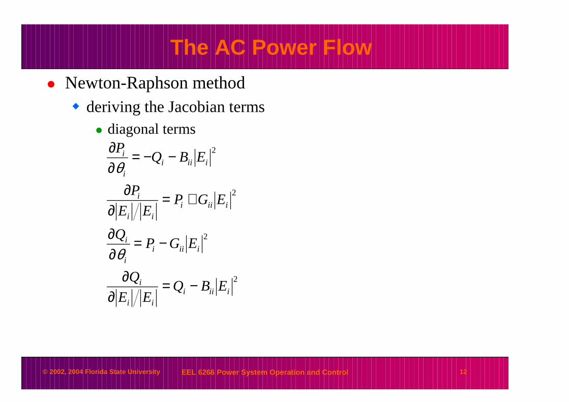
The AC Power Flow

� Newton-Raphson method� deriving the Jacobian terms

� diagonal terms

2

2

2

2

iiiiii

i

iiiii

i

iiiiii

i

iiiii

i

EBQEE

Q

EGPQ

EGPEE

P

EBQP

−=∂

∂

−=∂∂

+=∂

∂

−−=∂∂

θ

θ


The AC Power Flow

� Newton-Raphson method� solving the incremental equation

� gaussian elimination is often used to solve directly for the changes in voltage magnitudes and angles instead of finding the matrix inverse of the Jacobian explicitly

� the changes in voltage magnitudes and angles are added to the values that were used at the beginning of the iteration

[ ]

∆∆

∆∆

=

∆∆

∆∆

−

−

−−

n

n

nn

nn

Q

Q

P

P

J

EE

EE 1

2

1

1

11

2

1

MM

θθ


The AC Power Flow

� Newton-Raphson method� the solution process runs

according to the flowchart� note that the Jacobian

matrix is sparse

� the matrix algebra is carried out using Gaussianelimination or one of theother various numericalmethods

start

end

printresults

calculateline flows∆Pmax≤ε

∆Qmax≤ε

select initial voltage values

Newton-RaphsonPF Method

solve for ∆|E| and ∆θusing the Jacobian

and power mismatch

update voltagesθi

ξ+1= θiξ +∆θi

|Ei|ξ+1= |Ei|ξ+∆|Ei|

do for alli=1…N

i≠ref

calculate all ∆P & ∆Qform the Jacobian matrixfind max power mismatch


The AC Power Flow

� Example� three bus system

� solve the power flow Unit 165 MW1.02 pu

100 MW

Three Bus Network100 MVA base

Unit 21.05 pu

Bus 1

0.01 + j0.2

0.03 + j0.25

0.02 + j0.4

Bus 2

Bus 3


The AC Power Flow

� Non-linear system solution techniques� common solution methods

� fast-decoupled power flow� the Newton-Raphson is the most robust algorithm used in practice

� the Jacobian matrix must be recalculated for each iteration

� the set of linear equations must be resolved for each iteration

� a faster method was sought after

� simplifications in the Jacobian� in high voltage systems, the branch impedance is primarily

reactive, X >> R, X/R > 20• Bik >> Gik

� bus angles values are relatively close in value, |θi – θj| < 5°• cos(θi – θj) ≈ 1

• sin (θi – θj) ≈ 0


The AC Power Flow

� Fast Decoupled Power Flow� simplifications

� several of the off-diagonal terms tend towards zero

� the remaining off-diagonal terms can be reduced

( ) ( )( )

( ) ( )( ) 0sincos

0sincos

→=−+−−=∂∂

→=−+−=∂

∂

kiikkiikkik

i

kiikkiikkikk

i

BGEEQ

BGEEEE

P

θθθθθ

θθθθ

( ) ( )( )

( ) ( )( ) ikkikiikkiikkikk

i

ikkikiikkiikkik

i

BEEBGEEEE

Q

BEEBGEEP

−≈−−−=∂

∂

−≈−−−=∂∂

θθθθ

θθθθθ

cossin

cossin


The AC Power Flow


� several of the diagonal terms also tend towards zero

� the remaining diagonal terms can also be reduced

0

0

2

2

→=−=∂∂

→=+=∂

∂

iiiii

i

iiiiii

i

EGPQ

EGPEE

P

θ

22

22

2

iiiiiiiii

i

iiiiiiii

i

iiii

EBEBQEE

Q

EBEBQP

EBQ

−≈−=∂

∂

−≈−−=∂∂

<<

θ


The AC Power Flow


� taking into account the zero terms, the incremental corrections can be rewritten as

� substituting in the reduced terms

∑

∑

=

=

∆∂

∂=∆

∆∂∂=∆

N

k k

k

kk

ii

N

kk

k

ii

E

E

EE

QQ

PP

1

][

][

1

][][

ζζ

ζζ θθ

∑

∑

=

=

∆−=∆

∆−=∆

N

k k

k

ikkii

N

kkikkii

E

EBEEQ

BEEP

1

][

][

1

][][

ζζ

ζζ θ


The AC Power Flow

� Fast Decoupled Power Flow� further simplifications

� divide the terms by |Ei|

� assume |Ek| is approximately equal to one

� the equations in matrix form

∑

∑

=

=

∆−=∆

∆−=∆

N

kkik

i

i

N

kkik

i

i

EBE

Q

BE

P

1

][][

1

][][

ζζ

ζζ

θ

∆∆

−−−−

=

∆∆

−−−−

=

∆

∆

∆

∆

MOMM

L

L

MMOMM

L

L

M

][2

][1

2221

1211][

2

][1

2221

1211

2

][2

1

][1

2

][2

1

][1

ζ

ζ

ζ

ζ

ζ

ζ

ζ

ζ

θθ

E

E

BB

BB

BB

BB

EQ

EQ

EP

EP


The AC Power Flow

� Fast Decoupled Power Flow� resulting equations in general form

� where the terms in B´ and B" come from the susceptances of the bus admittance matrix terms

[ ]

[ ]

∆∆

′′=

∆∆

∆∆

′=

∆∆

MM

MM

2

1

22

11

2

1

22

11

E

E

BEQ

EQ

BEP

EP

θθ


The AC Power Flow

� Fast Decoupled Power Flow� advantages

� B´ and B" are constant� calculated once

� only B" may need to change, resulting from a generation VAR limit violation

� about 1/4 the number of terms found in the Jacobian

� disadvantages� solution convergence failure

� when underlying assumptions do not holdi.e., X/R > 20 and |θi – θj| < 5°


“DC” Power Flow

� A significant simplification of the power flow analysis� drop the Q-V equations altogether in the fast-decoupled

approach

� results in a completely linear, non-iterative power flow algorithm

� simply assume that all voltage magnitudes, |Ei|, equal 1.0 pu

� the system equation becomes

� the terms of B´ are as described for the fast decoupled method

[ ]

∆

∆∆

′=

∆

∆∆

NN

B

P

P

P

θ

θθ

MM

2

1

2

1


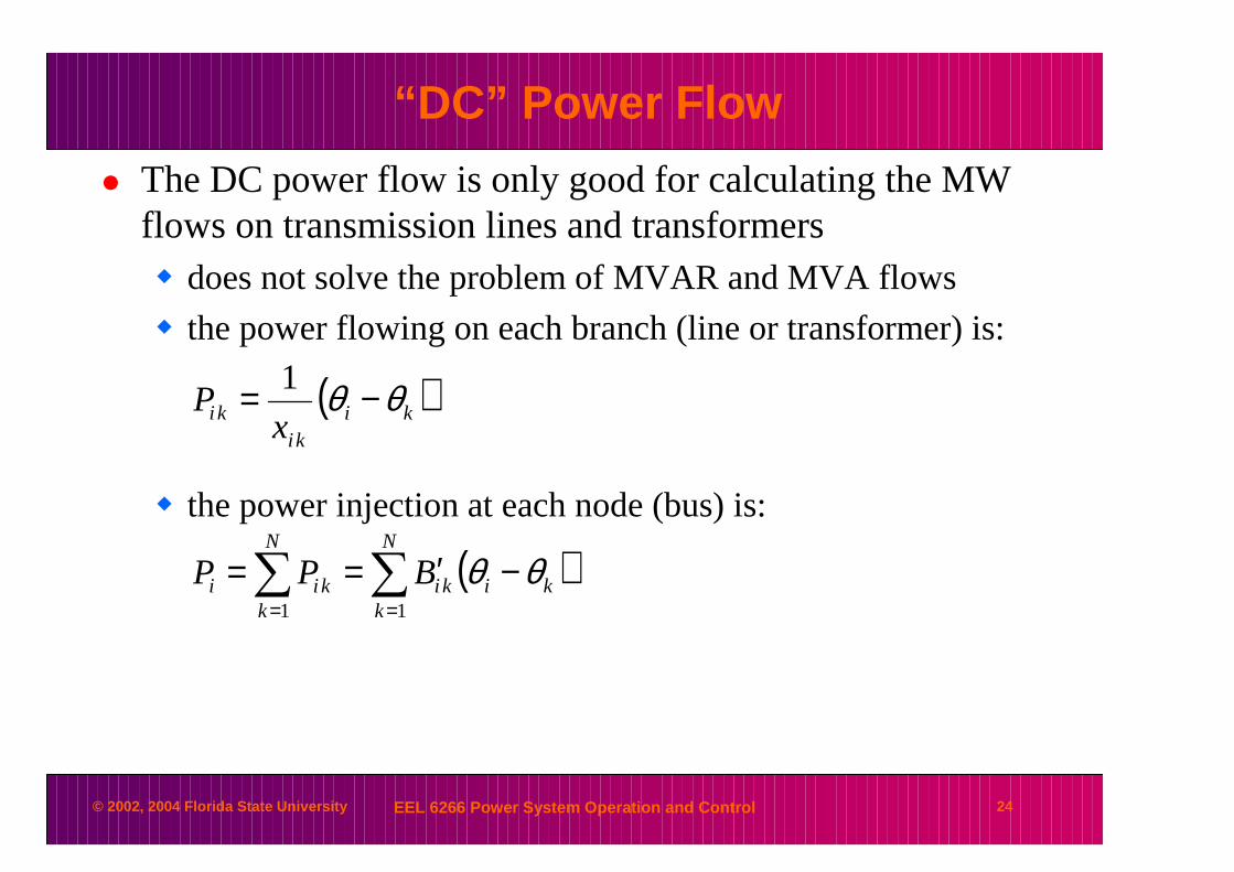
“DC” Power Flow

� The DC power flow is only good for calculating the MW flows on transmission lines and transformers� does not solve the problem of MVAR and MVA flows

� the power flowing on each branch (line or transformer) is:

� the power injection at each node (bus) is:

( )kiki

ki xP θθ −= 1

( )∑∑==

−′==N

kkiki

N

kkii BPP

11

θθ


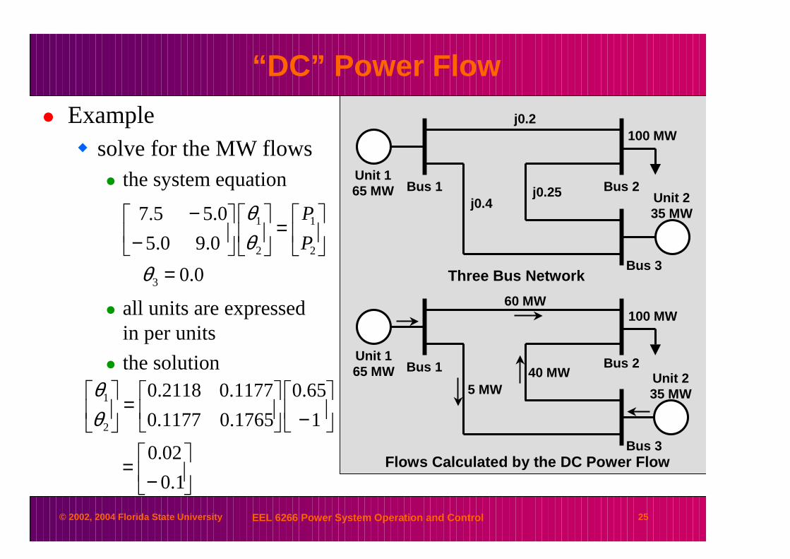
“DC” Power Flow

� Example� solve for the MW flows

� the system equation

� all units are expressedin per units

� the solution Unit 165 MW

Flows Calculated by the DC Power Flow

Unit 235 MW

Bus 1 Bus 2

Bus 3

Unit 165 MW

100 MW

60 MW

5 MW

Three Bus Network

Unit 235 MW

40 MW

Bus 1

j0.2

j0.25j0.4

Bus 2

Bus 3

100 MW

0.0

0.90.5

0.55.7

3

2

1

2

1

=

=

−−

θθθ

P

P

−=

−

=

1.0

02.0

1

65.0

1765.01177.0

1177.02118.0

2

1

θθ

Documents

EEL 6266 Power System Operation and Control · 2013-03-19 · EEL 6266 Power System Operation and Control Chapter 4 Transmission System Effects